Classification with unknown class-conditional label noise on non-compact feature spaces

Abstract

We investigate the problem of classification in the presence of unknown class-conditional label noise in which the labels observed by the learner have been corrupted with some unknown class dependent probability. In order to obtain finite sample rates, previous approaches to classification with unknown class-conditional label noise have required that the regression function is close to its extrema on sets of large measure. We shall consider this problem in the setting of non-compact metric spaces, where the regression function need not attain its extrema.

In this setting we determine the minimax optimal learning rates (up to logarithmic factors). The rate displays interesting threshold behaviour: When the regression function approaches its extrema at a sufficient rate, the optimal learning rates are of the same order as those obtained in the label-noise free setting. If the regression function approaches its extrema more gradually then classification performance necessarily degrades. In addition, we present an adaptive algorithm which attains these rates without prior knowledge of either the distributional parameters or the local density. This identifies for the first time a scenario in which finite sample rates are achievable in the label noise setting, but they differ from the optimal rates without label noise.

1 Introduction

In this paper we investigate the problem of classification with unknown class-conditional label noise on non-compact metric spaces. We determine minimax optimal learning rates which reveal an interesting dependency upon the behaviour of the regression function in the tails of the distribution.

Classification with label noise is a problem of great practical significance in machine learning. Whilst it is typically assumed that the train and test distributions are one and the same, it is often the case that the labels in the training data have been corrupted with some unknown probability Frénay and Verleysen (2014). We shall focus on the problem of class-conditional label noise, where the label noise depends on the class label (Bootkrajang and Kabán, 2014). This has numerous applications including learning from positive and unlabelled data (Elkan and Noto, 2008; Li et al., 2019) and nuclear particle classification Natarajan et al. (2013); Blanchard et al. (2016). Learning from class-conditional label noise is complicated by the fact that the optimal decision boundary will typically differ between test and train distributions. This effect can be accommodated for if the learner has prior knowledge of the label noise probabilities (the probability of flipping from one class to another) (Natarajan et al., 2013). Unfortunately, this is rarely the case in practice.

The seminal work of Scott et al. (2013) showed that the label noise probabilities may be consistently estimated from the data, under the mutual irreducibility assumption, which is equivalent to the assumption that the regression function $\eta$ has infimum zero and supremum one Menon et al. (2015). Without further assumptions the rate of convergence may be arbitrarily slow Blanchard et al. (2010); Scott et al. (2013); Blanchard et al. (2016). However, Scott (2015) demonstrated that a finite sample rate of order $O(1/\sqrt{n})$ may be obtained provided that the following strong irreducibility condition holds: There exists a family of sets $\mathcal{S}$ of finite VC dimension (eg. the set of metric balls in $\mathbb{R}^{d}$), such that for a pair of sets $S_{0}$, $S_{1}\in\mathcal{S}$ of positive measure, the regression function $\eta$ is uniformly zero on $S_{0}$ and uniformly one on $S_{1}$. Finite sample rates have also been obtained by Reeve and Kabán (2019) for the robust $k$-nearest neighbour classifier of Gao et al. (2018), with a strong uniform smoothness condition, in conjunction with the mutual irreducibility condition of Scott et al. (2013). In both cases, the learning rates for classification with unknown-class conditional label noise match the optimal rates for the corresponding label noise free setting, up to logarithmic terms. This motivates the question of whether there are scenarios in which finite sample rates are achievable in the label noise setting, yet the rates differ from the optimal rates without label noise?

In this work we focus on a flexible non-parametric setting which incorporates various natural examples where the marginal distribution is supported on a non-compact metric space. We will make a flexible tail assumption, due to Gadat et al. (2016), which controls the decay of the measure of regions of the feature space where the density is below a given threshold. This avoids the common yet restrictive assumption that the density is bounded uniformly from below or the assumption of finite covering dimension (Audibert et al., 2007). For non-compact metric spaces it is natural to consider settings where the regression function never attains its infimum and supremum, and instead approaches these values asymptotically, in the tails of the distribution. This occurs, for example, when the class-conditional distributions are mixtures of multivariate Gaussians. In this work we explore the relationship between the rate at which the regression function approaches its extrema and the optimal learning rates. Our contributions are as follows:

• We determine the minimax optimal learning rate (up to logarithmic factors) for classification in the presence of unknown class-conditional label noise on non-compact metric spaces (Theorems 3.1 and 4.6). The rate displays interesting threshold behaviour: When the regression function approaches its extrema at a sufficient rate, the optimal learning rates are of the same order as those obtained by Gadat et al. (2016) in the label-noise free setting. If the regression function approaches its extrema more gradually then classification performance necessarily degrades. This identifies, for the first time, a scenario in which finite sample rates are achievable in the label noise setting, but they differ from the rates achievable without label noise.

• We present an algorithm for classification with unknown class-conditional label noise on non-compact metric spaces. The algorithm is straightforward to implement and adaptive, in the sense that it does not require any prior knowledge of the distributional parameters or the local density. A high probability upper bound is proved which demonstrates that the performance of the algorithm is optimal, up to logarithmic factors (Theorem 4.6).

• As a byproduct of our analysis, we introduce a simple and adaptive method for estimating the maximum of a function on a non-compact domain. A high probability bound on its performance is given, with a rate governed by the local density at the maximum, if the maximum is attained, or the rate at which the function approaches its maximum otherwise (Theorem 4.2).

We begin by formalising the statistical setting in Section 2. We then present our minimax lower bound in Section 3. In Section 4 we introduce an adaptive algorithm with a high probability upper bound. Formal proofs may be found within the Appendix.

2 The statistical setting

We consider the problem of binary classification in metric spaces with class-conditional label noise. Suppose we have a metric space $\left(\mathcal{X},\rho\right)$, a set of possible labels $\mathcal{Y}=\{0,1\}$, and a distribution $\mathbb{P}$ over triples $(X,Y,\tilde{Y})\in\mathcal{X}\times\mathcal{Y}^{2}$, consisting of a feature vector $X\in\mathcal{X}$, a true class label $Y\in\mathcal{Y}$ and a corrupted label $\tilde{Y}\in\mathcal{Y}$, which may be distinct from $Y$. We let $\mathbb{P}_{\text{clean}}$ denote the marginal distribution over $(X,Y)$ and let $\mathbb{P}_{\text{corr}}$ denote the marginal distribution over $(X,\tilde{Y})$. Let $\mathcal{F}(\mathcal{X},\mathcal{Y})$ denote the set of all decision rules, which are Borel measureable mappings $\phi:\mathcal{X}\rightarrow\mathcal{Y}$. The goal of learner is to determine a decision rule $\phi\in\mathcal{F}(\mathcal{X},\mathcal{Y})$ which minimises the risk

$$\mathcal{R}\left(\phi\right):=\mathbb{P}_{\text{clean}}\left[\phi(X)\neq Y\right]=\int\left(\phi(x)\left(1-\eta(x)\right)+\left(1-\phi(x)\right)\eta(x)\right)d\mu(x)$$

Here $\eta:\mathcal{X}\rightarrow[0,1]$ denotes the regression function $\eta(x):=\mathbb{P}_{\text{clean}}\left[Y=1|X=x\right]$ and $\mu$ denotes the marginal distribution over $X$. The risk is minimised by the Bayes decision rule $\phi^{*}\in\mathcal{F}(\mathcal{X},\mathcal{Y})$ defined by $\phi^{*}(x):=\mathbbm{1}\left\{\eta(x)\geq\frac{1}{2}\right\}$. Since $\eta$ is unobserved, the learner must rely upon data. We assume that the learner has access to a corrupted sample ${\mathcal{D}}_{\text{corr}}=\{(X_{i},\tilde{Y}_{i})\}_{i\in[n]}$ where each $(X_{i},\tilde{Y}_{i})$ is sampled from $\mathbb{P}_{\text{corr}}$ independently. We let $(\mathbb{P}_{\text{corr}})^{\otimes n}$ denote the corresponding product distribution over samples ${\mathcal{D}}_{\text{corr}}$, and let $\mathbb{E}_{\text{corr}}^{\otimes n}$ denote expectation with respect to $(\mathbb{P}_{\text{corr}})^{\otimes n}$. The sample ${\mathcal{D}}_{\text{corr}}$ is utilised to train a classifier $\hat{\phi}_{n}$, which is a random member of $\mathcal{F}(\mathcal{X},\mathcal{Y})$, measurable with respect to ${\mathcal{D}}_{\text{corr}}$. The key difficulty of classification with label noise is that $\mathbb{P}_{\text{corr}}$ and $\mathbb{P}_{\text{clean}}$ may differ. Without further assumptions on the relationship between $\mathbb{P}_{\text{corr}}$ and $\mathbb{P}_{\text{clean}}$ the problem is clearly intractable. We utilise the assumption of class-conditional label noise introduced by Scott et al. (2013):

Assumption A (Class-conditional label noise)

We say that $\mathbb{P}$ satisfies the class-conditional label noise assumption with parameter $\nu_{\max}\in(0,1)$ if there exists $\pi_{0},\pi_{1}\in\left(0,1\right)$ with $\pi_{0}+\pi_{1}<\nu_{\max}$ such that for Borel sets $A\subset\mathcal{X}$, $\mathbb{P}[\tilde{Y}=1|X\in A,Y=0]=\pi_{0}$ and $\mathbb{P}[\tilde{Y}=0|X\in A,Y=1]=\pi_{1}$.

The remainder of our assumptions depend solely upon $\mathbb{P}_{\text{clean}}$ and are specified in terms of $\mu$ and $\eta$. We begin with two assumptions which are standard in the literature on non-parametric classification. The first is Tysbakov’s margin assumption Mammen and Tsybakov (1999).

Assumption B (Margin assumption)

Given $\alpha\in[0,\infty)$ and $C_{\alpha}\in[1,\infty)$, we shall say that $\mathbb{P}$ satisfies the margin assumption with parameters $\left(\alpha,C_{\alpha}\right)$ if the following holds for all $\xi\in(0,1)$,

$$\mu\left(\left\{x\in\mathcal{X}:0<\left|\eta(x)-\frac{1}{2}\right|<\xi\right\}\right)\leq C_{\alpha}\cdot\xi^{\alpha}.$$

We will also assume that the regression function $\eta$ is Hölder continuous.

Assumption C (Hölder assumption)

Given a function $f:\mathcal{X}\rightarrow[0,1]$ and constants $\beta\in(0,1]$, $C_{\beta}\geq 1$ we shall say that $f$ satisfies the Hölder assumption with parameters $(\beta,C_{\beta})$ if for all $x_{0},x_{1}\in\mathcal{X}$ with $\rho(x_{0},x_{1})<1$ we have $\left|f(x_{0})-f(x_{1})\right|\leq C_{\beta}\cdot\rho(x_{0},x_{1})^{\beta}$.

We shall also require some assumptions on $\mu$. We let $\mathcal{X}_{\mu}\subset\mathcal{X}$ denote the measure-theoretic support of $\mu$ and for each $x\in\mathcal{X}$ and $r\in(0,\infty)$ we let $B_{r}(x):=\left\{z\in\mathcal{X}:\rho(x,z)<r\right\}$.

Assumption D (Minimal mass assumption)

Given $d>0$ and a function $\omega_{\mu}:\mathcal{X}\rightarrow\left(0,1\right)$. We shall say that $\mu$ satisfies the minimal mass assumption with parameters $(d,\omega_{\mu})$ if we have $\mu\left(B_{r}(x)\right)\geq\omega_{\mu}(x)\cdot r^{d}$ for all $x\in\mathcal{X}_{\mu}$ and $r\in\left(0,1\right)$.

Assumption E (Tail assumption)

Given $\gamma\in(0,\infty)$, $C_{\gamma}\geq 1$, $t_{\gamma}\in(0,1)$ and a density function $\omega_{\mu}:\mathcal{X}\rightarrow\left(0,1\right)$, we shall say that $\mu$ satisfies the tail assumption with parameters $(\gamma,C_{\gamma},t_{\gamma},\omega_{\mu})$ if for all $\epsilon\in(0,t_{\gamma})$ we have $\mu\left(\left\{x\in\mathcal{X}:\omega_{\mu}(x)<\epsilon\right\}\right)\leq C_{\gamma}\cdot\epsilon^{\gamma}$.

Assumptions D and E are natural generalisations to metric spaces of the corresponding assumptions from Gadat et al. (2016) in the Euclidean setting. In particular, these assumptions apply to various examples such as Gaussian, Laplace and Cauchy distributions (Gadat et al., 2016, Table 1), with $\omega_{\mu}$ proportional to the probability density function.

Our final assumption is the most distinctive. It is a quantitative analogue of the mutual irreducibility assumption from (Scott et al., 2013) which implies that $\inf_{x\in\mathcal{X}_{\mu}}\left\{\eta(x)\right\}=0$ and
$\sup_{x\in\mathcal{X}_{\mu}}\left\{\eta(x)\right\}=1$. Rather than assume the existence of positive measure regions of the feature space upon which $\eta$ is uniformly zero and one, as required for the finite sample rates in (Scott, 2015, Theorem 2), (Blanchard et al., 2016, Theorem 14), we make a weaker assumption that governs the rate at which the regression function approaches its extrema in the tail of the distribution.

Assumption F (Quantitative range assumption)

Given $\tau\in(0,\infty)$, $C_{\tau}\geq 1$, $t_{\tau}\in(0,1)$ and a function $\omega_{\mu}:\mathcal{X}\rightarrow\left(0,1\right)$, we shall say that $\mathbb{P}$ satisfies the quantitative range assumption with parameters $\left(\tau,C_{\tau},t_{\tau},\omega_{\mu}\right)$ if for all $\epsilon\in(0,t_{\tau})$ we have

$$\max\left\{\inf_{x\in\mathcal{X}_{\mu}}\left\{\eta(x):\omega_{\mu}(x)>\epsilon\right\},\inf_{x\in\mathcal{X}_{\mu}}\left\{1-\eta(x):\omega_{\mu}(x)>\epsilon\right\}\right\}\leq C_{\tau}\cdot\epsilon^{\tau}.$$

If there are regions $S_{\min}\subset\mathcal{X}$ and $S_{\max}\subset\mathcal{X}$ with positive measure $\min\{\mu(S_{\min}),\mu(S_{\max})\}>0$ such that $\forall x\in S_{\min}$, $\eta(x)=0$ and $\forall x\in S_{\max}$, $\eta(x)=1$ then Assumption F holds with arbitrarily large $\tau>0$ (see Figure 1 (A)). More generally, if there exists $x_{\min},x_{\max}\in\mathcal{X}_{\mu}$ with $\min\{\omega_{\mu}(x_{\min}),\omega_{\mu}(x_{\min})\}>0$, $\eta(x_{\min})=0$ and $\eta(x_{\max})=1$ then Assumption F again holds with arbitrarily large $\tau>0$ (see Figure 1 (B)). However, Assumption F can also hold in scenarios in which the extrema of the regression function approaches its extrema gradually in the tails of the distribution. For example, consider a family of distributions $\{\mathbb{P}_{\tau}\}_{\tau>0}$ where for each $\tau$, $\mathbb{P}_{\tau}$ has a marginal distribution $\mu$ equal to the standard Laplace measure on $\mathbb{R}$ with probability density function $p(x)=\frac{1}{2}\cdot e^{-|x|}$ and regression function $\eta_{\tau}(x)=1/(1+e^{-\tau\cdot x})$ (see Figure 1 (C)). For each $\tau>0$, $\eta_{\tau}$ does not attain its extrema, yet Assumption F holds with exponent $\tau$. The exponent $\tau$ controls the rate at which the regression function approaches its extrema as the density function $\omega_{\mu}\approx p$ approaches zero.

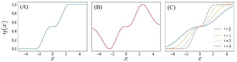
Figure 1: (A) An example of a regression function in which both the maximum and the minimum of $\eta$ are attained uniformly on sets of positive measure. (B) An example in which both the maximum and the minimum of $\eta$ are each attained at a single point. (C) A family of examples in which the regression function $\eta(x)=1/(1+e^{-\tau\cdot x})$ does not attain its extrema. The marginal distribution $\mu$ is the standard Laplace measure on $\mathbb{R}$ with density $p(x)=\frac{1}{2}\cdot e^{-|x|}$. In each case, Assumption F holds with the corresponding exponent $\tau$.

In what follows we consider the following class of distributions.

Definition 2.1 (Measure classes)

Take $\Gamma=(\nu_{\max},d,(\alpha,C_{\alpha}),(\beta,C_{\beta}),(\gamma,t_{\gamma},C_{\gamma}),(\tau,t_{\tau},C_{\tau}))$ consisting of exponents $\alpha\in[0,\infty)$, $\beta\in(0,1]$, $d$, $\gamma$, $\tau\in(0,\infty)$ and constants $C_{\alpha},C_{\beta},C_{\gamma},C_{\tau}\geq 1$ and $\nu_{\max}$, $t_{\gamma}$, $t_{\tau}\in(0,1)$. We let $\mathcal{P}\left(\Gamma\right)$ denote the set of all distributions $\mathbb{P}$ on triples $(X,Y,\tilde{Y})\in\mathcal{X}\times\mathcal{Y}^{2}$, where $(\mathcal{X},\rho)$ is a metric space and there is some function $\omega_{\mu}:\mathcal{X}\rightarrow(0,1)$ such Assumptions A, B, C, D, E, F hold with the corresponding parameters.

Now that we have introduced our assumptions we are ready to state our main results.

3 Minimax rates for classification with unknown class conditional label noise

Our first main result gives a minimax lower bound for classification with unknown class conditional label noise on non-compact domains.

Theorem 3.1.

Take $\Gamma=(\nu_{\max},d,(\alpha,C_{\alpha}),(\beta,C_{\beta}),(\gamma,t_{\gamma},C_{\gamma}),(\tau,t_{\tau},C_{\tau}))$ consisting of exponents $\alpha\in[0,\infty)$, $\beta\in(0,1]$, $d\in[\alpha\beta,\infty)$, $\gamma\in(0,1]$, $\tau\in(0,\infty)$ and constants $C_{\alpha}\geq 4^{\alpha}$, $C_{\beta}$, $C_{\gamma}$, $C_{\tau}\geq 1$ and $\nu_{\max}\in(0,1)$, $t_{\gamma}\in(0,1/24)$, $t_{\tau}\in(0,1/3)$. There exists a constant $c(\Gamma)>0$, depending solely upon $\Gamma$, such that for all $n\in\mathbb{N}$

$$\inf_{\hat{\phi}_{n}}\left\{\sup_{\mathbb{P}\in\mathcal{P}(\Gamma)}\left\{\mathbb{E}_{\text{corr}}^{\otimes n}\left[\mathcal{R}\left(\hat{\phi}_{n}\right)\right]-\mathcal{R}\left(\phi^{*}\right)\right\}\right\}\geq c(\Gamma)\cdot n^{-\min\left\{{\frac{\gamma\beta(\alpha+1)}{\gamma(2\beta+d)+\alpha\beta}},{\frac{\tau\beta(\alpha+1)}{\tau(2\beta+d)+\beta}}\right\}}.$$

The infimum is taken over all classifiers $\hat{\phi}_{n}$ which are measurable with respect to ${\mathcal{D}}_{\text{corr}}$.

In Section 4 we shall introduce a classifier which attains the rates in Theorem 3.1 up to logarithmic factors, with high-probability (Theorem 4.6). Theorem 3.1 displays an interesting threshold behaviour not seen in the label noise free setting. When the exponent $\tau$ is large ($\tau\cdot\alpha\geq\gamma$) and the regression function $\eta$ approaches its extrema sufficiently quickly, the exponent matches the label noise free rate. However, when the exponent $\tau$ is smaller ($\tau\cdot\alpha<\gamma$) and the regression function $\eta$ approaches its extrema more gradually, the learning behaviour deteriorates accordingly.

The proof of Theorem 3.1 reflects this threshold behaviour, and may be split into two claims:

$$\inf_{\hat{\phi}_{n}}\left\{\sup_{\mathbb{P}\in\mathcal{P}(\Gamma)}\left\{\mathbb{E}_{\text{corr}}^{\otimes n}\left[\mathcal{R}\left(\hat{\phi}_{n}\right)\right]-\mathcal{R}\left(\phi^{*}\right)\right\}\right\} \geq c_{0}(\Gamma)\cdot n^{-\frac{\beta\gamma(\alpha+1)}{\gamma(2\beta+d)+\alpha\beta}},$$ (1)

$$\inf_{\hat{\phi}_{n}}\left\{\sup_{\mathbb{P}\in\mathcal{P}(\Gamma)}\left\{\mathbb{E}_{\text{corr}}^{\otimes n}\left[\mathcal{R}\left(\hat{\phi}_{n}\right)\right]-\mathcal{R}\left(\phi^{*}\right)\right\}\right\} \geq c_{1}(\Gamma)\cdot n^{-\frac{\tau\beta(\alpha+1)}{\tau(2\beta+d)+\beta}}.$$ (2)

The lower bound in (1) corresponds to the difficulty of the pure classification problem, with or without label noise. The exponent is the same as that identified in (Gadat et al., 2016, Theorem 4.5). A full proof of claim (1) is presented in Appendix A.2 (Proposition 6). The proof method is broadly similar to that of Gadat et al. (2016), with two key differences. Firstly, our lower bounds hold for non-integer as well as integer dimension $d$. Secondly, technical adjustments are required to ensure that Assumption F is satisfied.

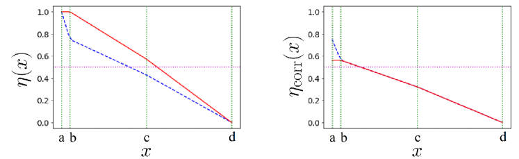
Figure 2: An illustration of the construction for the proof of Theorem 3.1 when $\tau\alpha\leq\gamma$. A pair of distributions with substantially different regression functions $\eta$ for which the corresponding corrupted regression functions ${\eta}_{\text{corr}}$ are close.

The lower bound in (2) corresponds to the difficulty of estimating the noise probabilities and the resultant effect upon classification risk. This component of the lower bound is more interesting as it reflects behaviour unseen in the label noise free setting. The proof of the lower bound in (2) is given in Appendix A.1 (Proposition 1). The idea is as follows. We construct a pair of distributions such that the corrupted regression functions closely resemble one another, yet the true regression functions are substantially different, and lie on different sides of the classification threshold $\frac{1}{2}$ for large fractions of the feature space. Thus, whilst it is difficult to distinguish the two distributions based upon the corrupted sample ${\mathcal{D}}_{\text{corr}}$, failing to do so results in substantial increase in risk relative to the Bayes classifier. The construction is illustrated in Figure 2.

4 An adaptive algorithm with a minimax optimal upper bound

In this section we construct a classifier for learning with unknown label noise on non-compact domains. In Section 4.4 we shall present high-probability performance guarantee for the algorithm (Theorem 4.6) which matches the minimax lower bound (Theorem 3.1) up to logarithmic factors.

4.1 Constructing an algorithm for classification with class conditional label noise

Our methodology is founded on observations due to Menon et al. (2015): Define ${\eta}_{\text{corr}}:\mathcal{X}\rightarrow[0,1]$ to be the corrupted regression function, given by ${\eta}_{\text{corr}}(x):=\mathbb{P}_{\text{corr}}[\tilde{Y}=1|X=x]$ for $x\in\mathcal{X}$. By Assumption A, ${\eta}_{\text{corr}}$ is related to $\eta$ by

$${\eta}_{\text{corr}}(x)=\left(1-\pi_{0}-\pi_{1}\right)\cdot\eta(x)+\pi_{0}.$$ (3)

Assumption F implies that $\inf_{x\in\mathcal{X}_{\mu}}\{\eta(x)\}=0$ and $\sup_{x\in\mathcal{X}_{\mu}}\{\eta(x)\}=1$. Combining with (3) yields $\inf_{x\in\mathcal{X}_{\mu}}\{{\eta}_{\text{corr}}(x)\}=\pi_{0}$ and $\sup_{x\in\mathcal{X}_{\mu}}\{{\eta}_{\text{corr}}(x)\}=1-\pi_{1}$. Moreover, relation (3) implies

$$\phi^{*}(x)=\mathbbm{1}\left\{\eta(x)\geq{1}/{2}\right\}=\mathbbm{1}\left\{{\eta}_{\text{corr}}(x)\geq({1}/{2})\cdot(1+\pi_{0}-\pi_{1})\right\}.$$

These observations motivate the ‘plug-in’ style template given in Algorithm 4.1. To instantiate Algorithm 4.1 in our setting we require a procedure for estimating the value of the corrupted regression function at a point ${\hat{\eta}}_{\text{corr}}(x)$ and a procedure for providing estimates $\hat{M}\left({{\eta}_{\text{corr}}}\right)$ and $\hat{M}\left(1-{{\eta}_{\text{corr}}}\right)$ for the supremum of ${\eta}_{\text{corr}}$ and $1-{\eta}_{\text{corr}}$, respectively, based on the corrupted sample ${\mathcal{D}}_{\text{corr}}$. Consequently, we turn to the subject of estimating the values of the corrupted regression function at a point in Section 4.2 and to the subject of estimating the extrema of the corrupted regression function in Section 4.3. In Section 4.4 we bring these pieces together to provide a concrete instantiation of Algorithm 4.1 with a high probability risk bound.

[htbp]

1. Compute an estimate of the corrupted regression function ${\hat{\eta}}_{\text{corr}}(x)$ with sample ${\mathcal{D}}_{\text{corr}}$;

2. Estimate $\hat{\pi}_{0}=1-\hat{M}\left(1-{\eta}_{\text{corr}}\right)$ and $\hat{\pi}_{1}=1-\hat{M}\left({{\eta}_{\text{corr}}}\right)$;

3. Let $\hat{\phi}(x):=\mathbbm{1}\left\{{\hat{\eta}}_{\text{corr}}(x)\geq 1/2\cdot\left(1+\hat{\pi}_{0}-\hat{\pi}_{1}\right)\right\}$.

A meta-algorithm for classification with class-conditional label noise.

4.2 Function estimation with k-nearest neighbours and Lepski’s rule

In this section we consider supervised $k$-nearest neighbour regression. Whilst we are motivated by the estimation of ${\eta}_{\text{corr}}$ we shall frame our results in a more general fashion for clarity. Suppose we have an unknown function $f:\mathcal{X}\rightarrow[0,1]$ and a distribution $\mathbb{P}_{f}$ on $\mathcal{X}\times[0,1]$ such that $f(x)=\mathbb{E}\left[Z|X=x\right]$ for all $x\in\mathcal{X}$. In this section we consider the task of to estimating $f$ based on a sample $\mathcal{D}_{f}=\left\{\left(X_{i},Z_{i}\right)\right\}_{i\in[n]}$ with $(X_{i},Z_{i})\sim\mathbb{P}_{f}$ generated i.i.d. Given $x\in\mathcal{X}$ we let $\left\{\tau_{n,q}(x)\right\}_{q\in[n]}$ be an enumeration of $[n]$ such that for each $q\in[n-1]$, $\rho\left(x,X_{\tau_{n,q}(x)}\right)\leq\rho\left(x,X_{\tau_{n,q+1}(x)}\right)$. The $k$-nearest neighbour regression estimator is given by

$$\hat{f}_{n,k}(x):=\frac{1}{k}\cdot\sum_{q\in[k]}Z_{\tau_{n,q}(x)}.$$

To apply $\hat{f}_{n,k}$ we must choose a value of $k$. The optimal value of $k$ will depend upon the distributional parameters and the local density $\omega_{\mu}(x)$ at a test point. Inspired by Kpotufe and Garg (2013) we shall use Lepski’s method to select $k$. For each $x\in\mathcal{X}$, $n\in\mathbb{N}$, $k\in[n]$ and $\delta\in(0,1)$ we define

$$\hat{\mathcal{I}}_{n,k,\delta}(x):=\left[\hat{f}_{n,k}(x)-\sqrt{\frac{2\log((4n)/\delta)}{k}},\hat{f}_{n,k}(x)+\sqrt{\frac{2\log((4n)/\delta)}{k}}\right].$$

We then let

$$\hat{k}_{n,\delta}(x):=\max_{k\in\mathbb{N}\cap[8\log(2n/\delta),n/2]}\left\{\bigcap_{q\in\mathbb{N}\cap[8\log(2n/\delta),k]}\hat{\mathcal{I}}_{n,q,\delta}(x)\neq\emptyset\right\},$$

and define $\hat{f}_{n,\delta}(x):=\hat{f}_{n,k}(x)$ with $k=\hat{k}_{n,\delta}(x)$. Intuitively, the value of $k$ is increased until the bias begins to dominate the variance, which reflects itself in non-overlapping confidence intervals.

Theorem 4.1.

Suppose that $f$ satisfies the Hölder assumption with parameters $(\beta,C_{\beta})$ and $\mu$ satisfies the minimal mass assumption with parameters $(d,\omega_{\mu})$. Given any $n\in\mathbb{N}$, $\delta\in(0,1)$ and $x\in\mathcal{X}$, with probability at least $1-\delta$ over $\mathcal{D}_{f}$ we have

$$\left|\hat{f}_{n,\delta}(x)-f(x)\right|\leq(8\sqrt{2})\cdot{C_{\beta}}^{\frac{d}{2\beta+d}}\cdot\left(\frac{\log(4n/\delta)}{\omega_{\mu}(x)\cdot n}\right)^{\frac{\beta}{2\beta+d}}.$$ (4)

A proof of Theorem 4.1 is presented in Appendix C. The principal difference with Kpotufe and Garg (2013) is that we do not require an upper bound on the $\epsilon$-covering numbers. This is crucial for our setting since the assumption of an upper bound on the $\epsilon$-covering numbers rules out interesting non-compact settings. Theorem 4.1 will be applied to the label noise problem in Section 4.4.

4.3 A lower confidence bound approach for estimating the supremum of a function

In this section we deal with the problem of estimating the supremum of a function $M(f):=\sup_{x\in\mathcal{X}_{\mu}}\{f(x)\}$. This is motivated by the challenge of estimating the label noise probabilities (Section 4.1). We adopt the general statistical setting from Section 4.2. One might expect to obtain an effective estimator of the maximum by simply taking the empirical maximum of $\hat{f}_{n,\delta}$ over the data. However, this approach is likely to overestimate the maximum in our non-compact setting since estimates at points with low density will have large variance. To mitigate this effect we must subtract a confidence interval. The error due to the variance of $\hat{f}_{n,k}(x)$ can be bounded via Hoeffding’s inequality. The error due to bias is more difficult to estimate since it depends upon unknown distributional parameters. Fortunately, for estimating $M(f)$ this is not a problem since the bias at any given point is always negative. This motivates the following simple adaptive estimator:

$$\hat{M}_{n,\delta}(f):=\max_{(i,k)\in[n]^{2}}\left\{\hat{f}_{n,k}(X_{i})-\sqrt{\frac{\log(4n/\delta)}{k}}\right\}.$$ (5)

Theorem 4.2.

Suppose that $f$ satisfies the Hölder assumption with parameters $(\beta,C_{\beta})$ and $\mu$ satisfies the minimal mass assumption with parameters $(d,\omega_{\mu})$. Given any $n\in\mathbb{N}$ and $\delta\in(0,1)$ with probability at least $1-\delta$ over $\mathcal{D}_{f}$ we have

$$\sup_{x\in\mathcal{X}_{\mu}}\left\{f(x)-7\cdot{C_{\beta}}^{\frac{d}{2\beta+d}}\cdot\left(\frac{\log(4n/\delta)}{\omega_{\mu}(x)\cdot n}\right)^{\frac{\beta}{2\beta+d}}\right\}\leq\hat{M}_{n,\delta}(f)\leq M(f).$$ (6)

Proof 4.3.

It suffices to show that for any fixed $x_{0}\in\mathcal{X}$ with probability at least $1-\delta$ over $\mathcal{D}_{f}$ we have

$$f(x_{0})-7\cdot{C_{\beta}}^{\frac{d}{2\beta+d}}\cdot\left(\frac{\log(4n/\delta)}{\omega_{\mu}(x_{0})\cdot n}\right)^{\frac{\beta}{2\beta+d}}\leq\hat{M}_{n,\delta}(f)\leq M(f).$$ (7)

Indeed, the bound (6) may then be deduced by continuity of measure.
Choose $\tilde{k}:=\lfloor\frac{1}{2}\cdot\left(\omega_{\mu}(x_{0})\cdot n\right)^{\frac{2\beta}{2\beta+d}}\cdot\left({\log(4n/\delta)}\cdot{C_{\beta}^{-2}}\right)^{{d}/{(2\beta+d)}}\rfloor$. By an application of the multiplicative Chernoff bound (Lemma 9), the following holds with probability at least $1-\delta/2$,

$$\rho\left(x_{0},X_{\tau_{n,\tilde{k}}(x)}\right)<\left(\frac{2\tilde{k}}{\omega_{\mu}(x_{0})\cdot n}\right)^{\frac{1}{d}}\leq\xi:=\left(\frac{\log(4n/\delta)}{C_{\beta}^{2}\cdot\omega_{\mu}(x_{0})\cdot n}\right)^{\frac{1}{2\beta+d}},$$ (8)

provided that $8\log(2n/\delta)\leq\tilde{k}\leq\omega_{\mu}(x_{0})\cdot n/2$. By Hoeffding’s inequality (see Lemma 10) combined with the union bound the following holds simultaneously over all pairs $(i,k)\in[n]^{2}$ with probability at least $1-\delta/2$,

$$\left|\hat{f}_{n,k}(X_{i})-\frac{1}{k}\sum_{q\in[k]}f\left(X_{\tau_{n,q}(X_{i})}\right)\right|<\sqrt{\frac{\log(2/(\delta/(2n^{2}))}{2k}}\leq\sqrt{\frac{\log(4n/\delta)}{k}}.$$ (9)

Let us assume that (8) and (9) hold. By the union bound this is the case with probability at least $1-\delta$. Now take $i_{0}=\tau_{n,1}(x_{0})\in[n]$. The upper bound in (7) follows immediately from (9).

To prove the lower bound in (7) we assume, without loss of generality, that $n$ is sufficiently large that $8\log(2n/\delta)\leq\tilde{k}\leq\omega_{\mu}(x_{0})\cdot n/2$ and $\tilde{k}\geq\frac{1}{4}\cdot\left(\omega_{\mu}(x_{0})\cdot n\right)^{\frac{2\beta}{2\beta+d}}\cdot\left({\log(4n/\delta)}\cdot{C_{\beta}^{-2}}\right)^{{d}/{(2\beta+d)}}$. Indeed the lower bound is trivial for smaller values of $n$. By (8) combined with the triangle inequality, for each $q\in[\tilde{k}]$ we have $\rho\left(X_{i_{0}},X_{\tau_{n,q}(x)}\right)\leq\rho\left(x_{0},X_{i_{0}}\right)+\rho\left(x_{0},X_{\tau_{n,q}(x)}\right)\leq 2\cdot\xi$, where $\xi$ is defined in (8). Hence, for each $q\in[\tilde{k}]$ we have $\rho\left(X_{i_{0}},X_{\tau_{n,q}(X_{i_{0}})}\right)\leq 2\cdot\xi$. Applying (8) once again we see that for all $q\in[\tilde{k}]$, we have $\rho\left(x_{0},X_{\tau_{n,q}(X_{i_{0}})}\right)\leq\rho\left(x_{0},X_{i_{0}}\right)+\rho\left(X_{i_{0}},X_{\tau_{n,q}(X_{i_{0}})}\right)\leq 3\cdot\xi$. By the Hölder assumption we deduce that

$$\left|\frac{1}{k}\sum_{q\in[\tilde{k}]}f\left(X_{\tau_{n,q}(X_{i_{0}})}\right)-f(x_{0})\right| \leq\max_{q\in[\tilde{k}]}\left\{C_{\beta}\cdot\rho\left(x_{0},X_{\tau_{n,q}(X_{i_{0}})}\right)^{\beta}\right\}$$

$$\leq C_{\beta}\cdot\left(3\cdot\xi\right)^{\beta}\leq 3\cdot{C_{\beta}}^{\frac{d}{2\beta+d}}\cdot\left(\frac{\log(4n/\delta)}{\omega_{\mu}(x_{0})\cdot n}\right)^{\frac{\beta}{2\beta+d}}.$$

Combining with (9) we deduce that

$$\hat{M}_{n,\delta}(f) \geq\hat{f}_{n,k}(X_{i_{0}})-f(x_{0})-\sqrt{\frac{\log(4n/\delta)}{\tilde{k}}}$$

$$\geq\frac{1}{k}\sum_{q\in[\tilde{k}]}f\left(X_{\tau_{n,q}(X_{i_{0}})}\right)-4\cdot\sqrt{\frac{\log(4n/\delta)}{4\tilde{k}}}$$

$$\geq f(x_{0})-3\cdot{C_{\beta}}^{\frac{d}{2\beta+d}}\cdot\left(\frac{\log(4n/\delta)}{\omega_{\mu}(x_{0})\cdot n}\right)^{\frac{\beta}{2\beta+d}}-4\cdot\sqrt{\frac{\log(4n/\delta)}{4\tilde{k}}}$$

$$\geq f(x_{0})-7\cdot{C_{\beta}}^{\frac{d}{2\beta+d}}\cdot\left(\frac{\log(4n/\delta)}{\omega_{\mu}(x_{0})\cdot n}\right)^{\frac{\beta}{2\beta+d}}.$$

This gives the lower bound in (7) and completes the proof of Theorem 4.2.

Theorem 4.2 implies the following corollary.

Corollary 4.4.

Suppose that $f$ satisfies the Hölder assumption with parameters $(\beta,C_{\beta})$ and $\mu$ satisfies the minimal mass assumption with parameters $(d,\omega_{\mu})$. Suppose further that for some $\tau\in(0,\infty]$, $C_{\tau}\geq 1$ and $t_{\tau}\in(0,1)$, for each $\epsilon\in(0,t_{\tau})$ we have $\sup_{x\in\mathcal{X}_{\mu}}\left\{f(x):\omega_{\mu}(x)>\epsilon\right\}\geq M(f)-C_{\tau}\cdot\epsilon^{\tau}$. Then, for each $n\in\mathbb{N}$ and $\delta\in(0,1)$ with probability at least $1-\delta$ over $\mathcal{D}_{f}$,

$$\left|\hat{M}_{n,\delta}(f)-M(f)\right|\leq 8\cdot\left(C_{\beta}^{d/\beta}\cdot(C_{\tau}/t_{\tau})\right)^{\frac{\beta}{2\beta+d}}\cdot\left(\frac{\log(4n/\delta)}{n}\right)^{\frac{\tau\beta}{\tau(2\beta+d)+\beta}}.$$

Proof 4.5.

Combine Theorem 4.2 with $\sup_{x\in\mathcal{X}_{\mu}}\left\{f(x):\omega_{\mu}(x)>\epsilon\right\}\geq M(f)-C_{\tau}\cdot\epsilon^{\tau}$ and

$$\epsilon=\min\left\{t_{\tau},\left(C_{\beta}^{d}/C_{\tau}^{2\beta+d}\right)^{\frac{1}{\tau(2\beta+d)+\beta}}\cdot\left(\frac{\log(4n/\delta)}{n}\right)^{\frac{\beta}{\tau(2\beta+d)+\beta}}\right\}.$$

Corollary 4.4 highlights the dependency of the maximum estimation method upon the rate at which the function approaches its maximum in the tails of the distribution.

4.4 A high-probability upper bound for classification with class conditional label noise

We now combine the procedures introduced in Sections 4.2 and 4.3 to instantiate the template given in Algorithm 4.1. Given a corrupted sample ${\mathcal{D}}_{\text{corr}}$ and a confidence parameter $\delta\in(0,1)$ proceed as follows: First, we estimate ${\eta}_{\text{corr}}(x)$ using the $k$-NN method introduced in Section 4.2 ${\hat{\eta}}_{\text{corr}}(x)=\widehat{\left({\eta}_{\text{corr}}\right)}_{n,\delta^{2}/3}(x)$. Second, we apply the maximum estimation procedure introduced in Section 4.3 to obtain estimates $\hat{\pi}_{0}=1-\hat{M}_{{n},{\delta/3}}\left(1-{\eta}_{\text{corr}}\right)$ and $\hat{\pi}_{1}=1-\hat{M}_{{n},{\delta/3}}\left({{\eta}_{\text{corr}}}\right)$. Third, we take $\hat{\phi}_{n,\delta}(x):=\mathbbm{1}\left\{{\hat{\eta}}_{\text{corr}}(x)\geq 1/2\cdot\left(1+\hat{\pi}_{0}-\hat{\pi}_{1}\right)\right\}$. The classifier $\hat{\phi}_{n,\delta}$ satisfies the high probability risk bound given in Theorem 4.6.

Theorem 4.6.

Take $\Gamma=(\nu_{\max},d,(\alpha,C_{\alpha}),(\beta,C_{\beta}),(\gamma,t_{\gamma},C_{\gamma}),(\tau,t_{\tau},C_{\tau}))$ consisting of exponents $\alpha\in[0,\infty)$, $\beta\in(0,1]$, $d\in(0,\infty)$, $\gamma\in(\beta/(2\beta+d),\infty)$, $\tau\in(0,\infty)$ and constants $\nu_{\max}\in(0,1)$, $C_{\alpha}$, $C_{\beta},C_{\gamma},C_{\tau}\geq 1$ and $t_{\gamma}$, $t_{\tau}\in(0,1)$. Then there exists a constant $C(\Gamma)$ depending solely upon $\Gamma$ such that for any $n\in\mathbb{N}$ and $\delta\in(0,1)$ the following risk bound holds with probability at least $1-\delta$ over the corrupted data sample ${\mathcal{D}}_{\text{corr}}$,

$$\mathcal{R}\left(\hat{\phi}_{n,\delta}\right)-\mathcal{R}\left(\phi^{*}\right)\leq C(\Gamma)\cdot\left(\frac{\log(n/\delta)}{n}\right)^{\min\left\{{\frac{\gamma\beta(\alpha+1)}{\gamma(2\beta+d)+\alpha\beta}},{\frac{\tau\beta(\alpha+1)}{\tau(2\beta+d)+\beta}}\right\}}+\delta.$$

A full proof of Theorem 4.6 is presented in Appendix B. By Theorem 3.1 the classifier $\hat{\phi}_{n,\delta}$ is minimax optimal up to logarithmic factor. We emphasise that the classifier $\hat{\phi}_{n,\delta}$ is fully adaptive and does not require any prior knowledge of either the local density $\omega_{\mu}(x)$, or the distributional parameters.

5 Related work

Classification with label noise

The problem of learning a classifier from data with corrupted labels has been widely studied (Frénay and Verleysen (2014)). Broadly speaking, there are two approaches to addressing this problem from a theoretical perspective. One approach is to assume that the label noise is either symmetric (but possibly instance dependent) or becomes symmetric as the regression function approaches $1/2$. In this setting the optimal decision boundary does not differ between test and train distributions and classical approaches such as $k$-nearest neighbours are consistent with finite sample rates Cannings et al. (2018); Menon et al. (2018). In turn, our focus is on class-conditional label noise for which the optimal decision boundary will typically differ between test and train distributions and classical algorithms will no longer be consistent. Natarajan et al. (2013) demonstrated that classification with class-conditional label noise is reducible to classification with a shifted threshold, provided that the noise probabilities are known. This method has been generalised to provide empirical risk minimisation based approaches for various objectives when one only has access to corrupted data Natarajan et al. (2018); van Rooyen and Williamson (2018). Scott (2015) demonstrated that the label noise probabilities may be estimated from the corrupted sample at a rate of $O(1/\sqrt{n})$ provided that there exists a family of sets $\mathcal{S}$ of finite VC dimension with $S_{0}$, $S_{1}\in\mathcal{S}$ such that $\min\{\mu(S_{0}),\mu(S_{1})\}>0$, $\forall x\in S_{0}$, $\eta(x)=0$ and $\forall x_{1}\in S_{1}$, $\eta(x_{1})=1$. This gives rise to a finite sample rate of $O(1/\sqrt{n})$ for classification with unknown label noise over hypothesis classes of bounded VC dimension (Scott, 2015; Blanchard et al., 2016). Ramaswamy et al. (2016) has provided an alternative approach to estimating label noise probabilities at a rate of $O(1/\sqrt{n})$. However, the bound requires a separability condition in a Hilbert space, which does not apply in our setting. Gao et al. (2018) gave an adaptation of the $k$-nearest neighbour ($k$-NN) method and prove convergence to the Bayes risk. Reeve and Kabán (2019) obtained minimax optimal fast rates for the method of Gao et al. (2018) under the measure smoothness assumptions of Chaudhuri and Dasgupta (2014); Döring et al. (2017) combined with the mutual irreducibility condition. In both (Scott, 2015; Blanchard et al., 2016) and (Reeve and Kabán, 2019) the assumptions ensure that the regression function is close to its extrema on sets of large measure. This implies that the statistical difficulty of estimating the label noise probabilities is dominated by the difficulty of the classification problem. Consequently, in both cases, the finite sample rates for classification with unknown label noise match the optimal rates for the corresponding label noise free setting, up to logarithmic terms (Blanchard et al., 2016; Reeve and Kabán, 2019). In this work we have studied a non-compact setting which includes examples where the minimax optimal rates for learning with label noise are strictly greater than those for learning without label noise.

Non-parametric classification in unbounded domains

The problem of non-parametric classification on non-compact domains where the marginal density is not bounded from below has received some recent attention. One approach is the measure-theoretic smoothness assumption of Chaudhuri and Dasgupta (2014); Döring et al. (2017) whereby deviations in the regression function are assumed to scale with the measure of metric balls. This means that the regression function must become increasingly smooth (i.e. smaller Lipschitz constant) as the density approaches zero. In this work we have adopted the less restrictive approach of Gadat et al. (2016) where the Lipschitz constant is not controlled by the density. Instead assumptions are made which bound the measure of the tail of the distribution (Assumption E). This more flexible setting includes natural examples (Gadat et al., 2016, Table 1) and results in optimal convergence rates which are provably slower than those achieved with densities bounded from below. The primary difference between our setting and that of Gadat et al. (2016) is that we allow for class-conditional label noise with unknown label noise probabilities. This requires alternative techniques and can result in different optimal rates (Theorems 3.1 and 4.6). In addition, our method is adaptive to the unknown distributional parameters and local density, unlike the local $k$-NN method of Gadat et al. (2016) which assumes prior knowledge of the local density at a test point. This adaptivity is especially significant in the label noise setting where one cannot tune hyper-parameters by minimising the classification error on a hold out set. In order to tune $k$ we use the Lepski method Lepski and Spokoiny (1997). Our use of the Lepski method is drawn from the work of Kpotufe and Garg (2013) who applied this method to kernel regression. The principal difference is that whereas Kpotufe and Garg (2013) establish a uniform bound which holds simultaneously for all test points, we only require a pointwise bound. The major advantage of this is that we are able to avoid the restrictive assumption of an upper bound on the $\epsilon$-covering numbers (which would rule out non-compact domains of interest). An alternative approach to non-compact domains has been pursued by Cannings et al. (2017). Whilst we follow Gadat et al. (2016) in bounding the measure of the regions of the feature space where the density falls below a given value (see Assumption E), Cannings et al. (2017) instead employ a moment assumption. Note that whereas Cannings et al. (2017) make use of an additional set of unlabelled data to locally tune the optimal value of $k$, our method is optimally adaptive without any additional data.

Supremum estimation

Central to our method is the observation of Menon et al. (2015) that under the mutual irreducibility assumption the noise probabilities may be determined by estimating the extrema of the corrupted regression function. This leads to the problem of determining the supremum of a function on an unbounded metric space based on labelled data. This is closely related to the problem of mode estimation studied by Dasgupta and Kpotufe (2014) in an unsupervised setting and by Jiang (2019) in a supervised setting. The primary difference is that whereas we are only interested in estimating the value of the supremum, those papers focus on estimating the point in the feature space which attains the supremum. This is a more challenging problem which requires strong assumptions including a twice differentiable function. In our setting the feature space is not assumed to have a differentiable structure, so such assumptions cannot be applied. Note also that the sup norm bound of Jiang (2019) does not hold in our setting since it requires a uniform lower bound on the density. Our problem is also related to the simple regret minimisation problem in $\mathcal{X}$-armed bandits Bubeck et al. (2011); Locatelli and Carpentier (2018) in which the learner actively selects points in the feature space in order to locate and determine the supremum. However, the techniques are quite different, owing to the active rather than passive nature of the problem. In particular, there is no marginal distribution over the feature vectors, since these are selected by the learner. In our setting, conversely, the behaviour of the marginal distribution plays an absolutely crucial role.

6 Conclusion

We have determined the minimax optimal learning rate (up to logarithmic factors) for classification in the presence of unknown class-conditional label noise on non-compact metric spaces. The rate displayed an interesting threshold behaviour depending upon the rate at which the regression function approaches its extrema in the tails of the distribution. In addition, we presented an adaptive classification algorithm that attains the minimax rates without prior knowledge of the distributional parameters or the local density.

This work is funded by EPSRC under Fellowship grant EP/P004245/1. The authors would like to thank Nikolaos Nikolaou and Timothy I. Cannings for useful discussions. We would also like to thank the anonymous reviewers for their careful feedback which led to several improvements in the presentation.

Appendix A Proof of the lower bound

In this section we shall present the proof of the main lower bound - Theorem 3.1. The proof of Theorem 3.1 consists of two components. The first component corresponds to the difficulty of estimating the noise probabilities and the resultant effect upon classification risk. This component is presented in Proposition 1 in Section A.1. The second component corresponds to the difficulty of the core classification problem which would have been present even if the learner had access to clean labels. This component is presented in Proposition 6 in Section A.2. Theorem 3.1 follows immediately from Propositions 1 and 6.

Before presenting Propositions 1 and 6 we shall remind the reader of some notation that will be useful in the proof of the lower bound. Recall that we have a distribution $\mathbb{P}$ over triples $(X,Y,\tilde{Y})$. We let $\mathbb{P}_{\text{clean}}$ denote the marginal distribution over $(X,Y)$ and $\mathbb{P}_{\text{corr}}$ denote the marginal distribution over $(X,\tilde{Y})$. In addition, we let $\mathbb{P}_{\text{clean}}^{\otimes n}$ denote the product distribution over clean samples $\mathcal{D}=\{(X_{i},Y_{i})\}_{i\in[n]}$ with $(X_{i},Y_{i})$ sampled from $\mathbb{P}_{\text{clean}}$ independently and let $\mathbb{P}_{\text{corr}}^{\otimes n}$ denote the product distribution over corrupted samples ${\mathcal{D}}_{\text{corr}}=\{(X_{i},\tilde{Y}_{i})\}_{i\in[n]}$ with $(X_{i},\tilde{Y}_{i})$ sampled from $\mathbb{P}_{\text{corr}}$. Similarly, we let $\mathbb{E}_{\text{clean}}^{\otimes n}$ denote the expectation over clean samples $\mathcal{D}\sim\mathbb{P}_{\text{clean}}^{\otimes n}$ and let $\mathbb{E}_{\text{corr}}^{\otimes n}$ denote the expectation over corrupted samples ${\mathcal{D}}_{\text{corr}}\sim\mathbb{P}_{\text{corr}}^{\otimes n}$.

A.1 A lower bound for unknown label noise

The goal of this section is to prove Proposition 1 which corresponds to the difficulty of estimating the noise probabilities and the resultant effect upon classification risk.

Proposition 1.

Take $\Gamma=(\nu_{\max},d,(\alpha,C_{\alpha}),(\beta,C_{\beta}),(\gamma,t_{\gamma},C_{\gamma}),(\tau,t_{\tau},C_{\tau}))$ consisting of exponents $\alpha\in[0,\infty)$, $\beta\in(0,1]$, $d\in[\alpha\beta,\infty)$, $\gamma\in(0,1]$, $\tau\in(0,\infty)$ and constants $\nu_{\max}\in(0,1)$, $C_{\alpha}\geq 4^{\alpha}$, $C_{\alpha}$, $C_{\beta}$, $C_{\gamma}$, $C_{\tau}\geq 1$ and $t_{\gamma}\in(0,1/24)$, $t_{\tau}\in(0,1/3)$. There exists a constant $c_{0}(\Gamma)$, depending solely upon $\Gamma$, such that for any $n\in\mathbb{N}$ and any classifier $\hat{\phi}_{n}$ which is measurable with respect to the corrupted sample ${\mathcal{D}}_{\text{corr}}$, there exists a distribution $\mathbb{P}\in\mathcal{P}(\Gamma)$ such that

$$\mathbb{E}_{\text{corr}}^{\otimes n}\left[\mathcal{R}\left(\hat{\phi}_{n}\right)\right]-\mathcal{R}\left(\phi^{*}\right)\geq c_{1}(\Gamma)\cdot n^{-\frac{\tau\beta(\alpha+1)}{\tau(2\beta+d)+\beta}}.$$

To prove Proposition 1 we will show that there exists a pair of distributions $\mathbb{P}^{0}$ and $\mathbb{P}^{1}$ such that whilst the corrupted regression functions (${\eta}_{\text{corr}}^{0}$ and ${\eta}_{\text{corr}}^{1}$) closely resemble one another, the true regression functions ($\eta^{0}$ and $\eta^{1}$) are substantially different. Thus, whilst it is difficult to distinguish $\mathbb{P}^{0}$ and $\mathbb{P}^{1}$ based upon the corrupted sample ${\mathcal{D}}_{\text{corr}}$, failing to do so results in substantial misclassification error. Figure 2 in Section 3 illustrates the construction. To formalise this idea we require the following variant of Fano’s lemma due to Birgé (2001).

Lemma 2 (Birgé).

Given a finite family $\mathcal{S}$ consisting of probability measures on a measureable space $\left(\mathcal{Z},\Sigma\right)$ and a random variable $Z$ with an unknown distribution in the family, then we have

$$\inf_{\hat{T}}\left\{\sup_{{\mathbb{P}}_{Z}\in\mathcal{S}}\left\{\mathbb{P}_{Z}\left[\hat{T}(Z)\neq\mathbb{P}_{Z}\right]\right\}\right\}\geq\min\left\{0.36,1-\inf_{\mathbb{P}_{Z}\in\mathcal{S}}\left\{\sum_{\tilde{\mathbb{P}}_{Z}\in\mathcal{S}}\frac{D_{KL}\left(\mathbb{P}_{Z},\tilde{\mathbb{P}}_{Z}\right)}{\left|\mathcal{S}\right|\log\left|\mathcal{S}\right|}\right\}\right\},$$

where the infimum is taken over all measureable (possibly randomised) estimators $\hat{T}:\mathcal{Z}\rightarrow\mathcal{S}$.

We apply Lemma 2 as follows: Given an integer $n\in\mathbb{N}$ and a quintuple $\left(\Delta,r,u,v,w\right)\in(0,1/6)^{5}$ (to be selected in terms of $n$ later) we shall construct a measureable space with a pair of distributions. First we construct a metric space by letting $\mathcal{X}=\{a,b,c,d\}$ and choosing $\rho$ such that

$$\rho(x_{0},x_{1}) =r x_{0},x_{1}\in\{a,b\}\text{ and }x_{0}\neq x_{1}$$ if

$$\rho(x_{0},x_{1}) \geq 1 x_{0}\notin\{a,b\}\text{ or }x_{1}\notin\{a,b\}\text{ and }x_{0}\neq x_{1}$$ if

$$\rho(x_{0},x_{1}) =0 x_{0}=x_{1}.$$ if

Note that there are metric spaces $(\mathcal{X},\rho)$ of this form embedded isometrically in any Euclidean space $(\mathbb{R}^{D},\|\cdot\|_{2})$. We shall define a pair of probability distributions $\mathbb{P}^{0},\mathbb{P}^{1}$ over random triples $(X,Y,\tilde{Y})\in\mathcal{X}\times\mathcal{Y}^{2}$ as follows. First we define a Borel probability measure $\mu$ on $\mathcal{X}$ by $\mu(\{a\})=u$, $\mu(\{b\})=1/3$, $\mu(\{c\})=v$ and $\mu(\{d\})=2/3-u-v$. Second, we define a pair of regression functions $\eta^{0},\eta^{1}:\mathcal{X}\rightarrow[0,1]$ on $\mathcal{X}$ as follows by

$$\eta^{0}(a) =1, \hskip 28.45274pt\eta^{0}(b) =1-\Delta, \hskip 28.45274pt\eta^{0}(c) =\frac{1-\Delta}{2-\Delta} \hskip 28.45274pt\eta^{0}(d) =0$$

$$\eta^{1}(a) =1, \eta^{1}(b) =1, \eta^{1}(c) =\frac{1}{2-\Delta} \eta^{1}(d) =0.$$

Third, we define probabilities $\pi_{j}^{\iota}\in(0,1)$ for $\{\iota,j\}\in\{0,1\}$ by taking $\pi_{0}^{0}=\pi_{1}^{0}=0$, $\pi_{1}^{0}=\nu_{\max}/4$ and $\pi_{1}^{1}=\Delta+(\nu_{\max}/4)\cdot(1-\Delta)$. We then put these pieces together by taking, for each ${\iota}\in\{0,1\}$, $\mathbb{P}^{\iota}$ to be the unique distribution on $(X,Y,\tilde{Y})\in\mathcal{X}\times\mathcal{Y}^{2}$ with (a) marginal distribution $\mu$, (b) regression function $\eta^{\iota}(x)=\mathbb{P}^{\iota}[Y=1|X=x]$ and (c) label noise probabilities $\pi_{j}^{\iota}$. In addition, we define $\omega_{\mu}:\mathcal{X}\rightarrow(0,1)$ by $\omega_{\mu}(a)=w$, $\omega_{\mu}(c)=v$ and $\omega_{\mu}(b)=\omega_{\mu}(d)=1/3$.

Lemma 3.

For $\iota\in\{0,1\}$ the measures $\mathbb{P}^{\iota}$ satisfy the following properties:

1. $\mathbb{P}^{\iota}$ satisfies Assumption A with parameter $\nu_{\max}$ provided $\Delta\leq\nu_{\max}/2$;

2. $\mathbb{P}^{\iota}$ satisfies Assumption B with parameters $(\alpha,C_{\alpha})$ whenever $C_{\alpha}\geq 4^{\alpha}$ & $v\leq\Delta^{\alpha}$;

3. $\eta^{\iota}$ satisfies Assumption C with parameters $(\beta,C_{\beta})$ whenever $\Delta\leq C_{\beta}\cdot r^{\beta}$;

4. $\mu$ satisfies Assumption D with parameters $(d,\omega_{\mu})$ whenever $u\geq w\cdot r^{d}$;

5. $\mu$ satisfies Assumption E with parameters $(\gamma,C_{\gamma},t_{\gamma},\omega_{\mu})$ whenever $\gamma\leq 1$, $t_{\gamma}\leq\frac{1}{3}$ & $u\leq w$;

6. $\mathbb{P}^{\iota}$ satisfies Assumption F with parameters $(\tau,C_{\tau},t_{\tau},\omega_{\mu})$ whenever $t_{\tau}\leq 1/3$ & $\Delta\leq C_{\tau}\cdot w^{\tau}$.

Proof A.1.

We check each property in turn.

Property A follows immediately from the construction of $\mathbb{P}^{\iota}$ and the definitions of $\pi_{j}^{\iota}$.

Property B follows from the fact that since $\Delta<1/6$, we have $\left|\eta^{\iota}(x)-1/2\right|\geq 1/3$ for $x\neq c$ and $\left|\eta^{\iota}(c)-1/2\right|\geq\Delta/4$. Property C follows from the fact that the only two distinct points $x_{0},x_{1}$ with $\rho(x_{0},x_{1})<1$ are $a$ & $b$ with $\rho(a,b)=r$ and $\left|\eta^{\iota}(a)-\eta^{\iota}(b)\right|\leq\Delta$.

Property D follows from the fact that $\mu$ is defined by $\mu(\{a\})=u$, $\mu(\{b\})=1/3$, $\mu(\{c\})=v$, $\mu(\{d\})=2/3-u-v$ and $\omega_{\mu}:\mathcal{X}\rightarrow(0,1)$ by $\omega_{\mu}(a)=w$, $\omega_{\mu}(c)=v$ and $\omega_{\mu}(b)=\omega_{\mu}(d)=1/3$. In particular, for $x\neq a$ we have for $\tilde{r}\in(0,1)$

$$\mu(B_{\tilde{r}}(x))\geq\mu(\{x\})\geq\omega_{\mu}(x)\geq\omega_{\mu}(x)\cdot{\tilde{r}}^{d}.$$

On the other hand, for $x=a$ there are two cases. If ${\tilde{r}}\in(r,1)$ then

$$\mu(B_{\tilde{r}}(a))\geq\mu(\{b\})\geq 1/3\geq w\cdot{\tilde{r}}^{d}=\omega_{\mu}(a)\cdot{\tilde{r}}^{d}$$

since $w<1/6$. If ${\tilde{r}}\leq r$ then $\mu(B_{\tilde{r}}(a))\geq\mu(\{a\})=u\geq w\cdot r^{d}\geq\omega_{\mu}(a)\cdot{\tilde{r}}^{d}$.

Property E requires three cases. If $\epsilon\in[\max\{w,v\},1/3)$ then we have

$$\mu\left(\{x\in\mathcal{X}:\omega_{\mu}(x)<\epsilon\}\right)=\mu\left(\{a,c\}\right)=u+v\leq 2\max\{w,v\}\leq C_{\gamma}\cdot\epsilon^{\gamma}.$$

If $\epsilon\in[\min\{w,v\},\max\{w,v\})$ then we take $x_{0}\in\{a,c\}$ with $\omega_{\mu}(x_{0})=\min_{x\in\mathcal{X}}\{\omega_{\mu}(x)\}$. Since $u\leq w$ we have

$$\mu\left(\{x\in\mathcal{X}:\omega_{\mu}(x)<\epsilon\}\right)=\mu\left(\{x_{0}\}\right)\leq\omega_{\mu}(x_{0})=\min\{w,v\}\leq\epsilon\leq C_{\gamma}\cdot\epsilon^{\gamma}.$$

Finally, for $\epsilon\in(0,\min\{w,v\})$ we have $\mu\left(\{x\in\mathcal{X}:\omega_{\mu}(x)<\epsilon\}\right)=0$.

Property F requires us to consider two cases. If $\epsilon\in[w,t_{\tau})$ then since $\omega_{\mu}(b)=\omega_{\mu}(d)=1/3>\epsilon$ and for both $\iota\in\{0,1\}$ we have $\eta^{\iota}(b)\geq 1-\Delta$ and $\eta^{\iota}(d)=0$ we have

$$\max\left\{\inf_{x\in\mathcal{X}_{\mu}}\left\{\eta^{\iota}(x):\omega_{\mu}(x)>\epsilon\right\},\inf_{x\in\mathcal{X}_{\mu}}\left\{1-\eta^{\iota}(x):\omega_{\mu}(x)>\epsilon\right\}\right\}\leq\Delta\leq C_{\tau}\cdot\epsilon^{\tau}.$$

On the other hand, if $\epsilon\in(0,w)$ then since $\omega_{\mu}(a)=w$ and $\eta^{\iota}(a)=1$, and $\eta^{\iota}(d)=0$ we have

$$\max\left\{\inf_{x\in\mathcal{X}_{\mu}}\left\{\eta^{\iota}(x):\omega_{\mu}(x)>\epsilon\right\},\inf_{x\in\mathcal{X}_{\mu}}\left\{1-\eta^{\iota}(x):\omega_{\mu}(x)>\epsilon\right\}\right\}=0\leq C_{\tau}\cdot\epsilon^{\tau}.$$

Recall that $\left({\mathbb{P}}_{\text{corr}}^{\iota}\right)^{\otimes n}$ is the product distribution with ${\mathcal{D}}_{\text{corr}}\sim\left({\mathbb{P}}_{\text{corr}}^{\iota}\right)^{\otimes n}$.

Lemma 4.

$\max\left\{D_{KL}\left(\left({\mathbb{P}}_{\text{corr}}^{0}\right)^{\otimes n},\left({\mathbb{P}}_{\text{corr}}^{1}\right)^{\otimes n}\right),D_{KL}\left(\left({\mathbb{P}}_{\text{corr}}^{1}\right)^{\otimes n},\left({\mathbb{P}}_{\text{corr}}^{0}\right)^{\otimes n}\right)\right\}\leq\frac{4nu\Delta^{2}}{\nu_{\max}}$.

Proof A.2.

We shall show that $D_{KL}\left(\left({\mathbb{P}}_{\text{corr}}^{0}\right)^{\otimes n},\left({\mathbb{P}}_{\text{corr}}^{1}\right)^{\otimes n}\right)\leq(4/\nu_{\max})\cdot nu\cdot\Delta^{2}$. The proof that
$D_{KL}\left(\left({\mathbb{P}}_{\text{corr}}^{1}\right)^{\otimes n},\left({\mathbb{P}}_{\text{corr}}^{0}\right)^{\otimes n}\right)\leq(4/\nu_{\max})\cdot nu\cdot\Delta^{2}$ is similar. Recall that for each ${\iota}\in\{0,1\}$ we let ${\mathbb{P}}_{\text{corr}}^{\iota}$ denote the marginal distribution of $\mathbb{P}^{\iota}$ over pairs $(X,\tilde{Y})$ consisting of a feature vector $X\sim\mathcal{X}$ and a corrupted label $\tilde{Y}\in\mathcal{Y}$. We can compute the corrupted regression functions ${\eta}_{\text{corr}}^{\iota}(x)=\mathbb{P}^{\iota}[\tilde{Y}|X=x]$ for ${\iota}\in\{0,1\}$ by applying (3). Since $\pi_{0}^{0}=0$ and $\pi_{1}^{0}=\nu_{\max}/4$ we have ${\eta}_{\text{corr}}^{0}(x)=(1-\nu_{\max}/4)\cdot\eta^{0}(x)$ for all $x\in\mathcal{X}$. On the other hand, since $\pi_{0}^{1}=0$ and $\pi_{1}^{1}=\Delta+(\nu_{\max}/4)\cdot(1-\Delta)$ we have ${\eta}_{\text{corr}}^{1}(x)=(1-\nu_{\max}/4)\cdot(1-\Delta)\cdot\eta^{1}(x)$ for all $x\in\mathcal{X}$.

We begin by bounding the Kullback Leibler divergence between ${\mathbb{P}}_{\text{corr}}^{0}$ and ${\mathbb{P}}_{\text{corr}}^{1}$ using the fact that $\mu(\{a\})=u$ and ${\eta}_{\text{corr}}^{0}(x)={\eta}_{\text{corr}}^{1}(x)$ for $x\in\mathcal{X}\backslash\{a\}$,

$$D_{KL}\left({\mathbb{P}}_{\text{corr}}^{0},{\mathbb{P}}_{\text{corr}}^{1}\right) =\sum_{x\in\mathcal{X}}\sum_{y\in\mathcal{Y}}{\mathbb{P}}_{\text{corr}}^{0}\left[X=x\hskip 5.69054pt\&\hskip 5.69054pt\tilde{Y}=y\right]\log\left(\frac{{\mathbb{P}}_{\text{corr}}^{0}\left[X=x\hskip 5.69054pt\&\hskip 5.69054pt\tilde{Y}=y\right]}{{\mathbb{P}}_{\text{corr}}^{1}\left[X=x\hskip 5.69054pt\&\hskip 5.69054pt\tilde{Y}=y\right]}\right)$$

$$=\sum_{x\in\mathcal{X}}\mu(\{x\})\left((1-{\eta}_{\text{corr}}^{0}(x))\log\left(\frac{1-{\eta}_{\text{corr}}^{0}(x)}{1-{\eta}_{\text{corr}}^{1}(x)}\right)+{\eta}_{\text{corr}}^{0}(x)\log\left(\frac{{\eta}_{\text{corr}}^{0}(x)}{{\eta}_{\text{corr}}^{1}(x)}\right)\right)$$

$$=u\cdot\left((1-{\eta}_{\text{corr}}^{0}(a))\log\left(\frac{1-{\eta}_{\text{corr}}^{0}(a)}{1-{\eta}_{\text{corr}}^{1}(a)}\right)+{\eta}_{\text{corr}}^{0}(a)\log\left(\frac{{\eta}_{\text{corr}}^{0}(a)}{{\eta}_{\text{corr}}^{1}(a)}\right)\right)$$

$$\leq u\cdot\frac{\left({\eta}_{\text{corr}}^{0}(a)-{\eta}_{\text{corr}}^{1}(a)\right)^{2}}{\min\left\{{\eta}_{\text{corr}}^{0}(a),(1-{\eta}_{\text{corr}}^{0}(a)),{\eta}_{\text{corr}}^{1}(a),1-{\eta}_{\text{corr}}^{1}(a)\right\}}\leq\frac{4}{\nu_{\max}}\cdot u\cdot\Delta^{2}.$$

The second to last inequality follows from the reverse Pinsker’s inequality (Csiszár and Talata, 2006, Lemma 6.3). The final inequality follows from the fact that ${\eta}_{\text{corr}}^{0}(a)=(1-{\nu_{\max}}/{4})$ and ${\eta}_{\text{corr}}^{1}(a)=(1-{\nu_{\max}}/{4})\cdot(1-\Delta)$. Given that $\left({\mathbb{P}}_{\text{corr}}^{\iota}\right)^{\otimes n}$ consists of $n$ independent copies of ${\mathbb{P}}_{\text{corr}}^{\iota}$ for $\iota\in\{0,1\}$ we deduce that

$$D_{KL}\left(\left({\mathbb{P}}_{\text{corr}}^{0}\right)^{\otimes n},\left({\mathbb{P}}_{\text{corr}}^{1}\right)^{\otimes n}\right)=n\cdot D_{KL}\left({\mathbb{P}}_{\text{corr}}^{0},{\mathbb{P}}_{\text{corr}}^{1}\right)\leq\frac{4nu\Delta^{2}}{\nu_{\max}}.$$

Lemma 5.

Suppose that $8nu\cdot\Delta^{2}\leq\nu_{\max}$. Given any ${\mathcal{D}}_{\text{corr}}$-measureable classifier $\hat{\phi}_{n}$,

$$\sum_{\iota\in\{0,1\}}\left(\mathbb{E}_{\text{corr}}^{\otimes n}\left[\mathcal{R}\left(\hat{\phi}_{n}\right)\right]-\mathcal{R}\left(\phi^{*}\right)\right)\geq\frac{v\cdot\Delta}{8}.$$

Proof A.3.

By Lemma 4 combined with $8nu\cdot\Delta^{2}\leq\nu_{\max}$ we have

$$(2\log 2)^{-1}\cdot\max\left\{D_{KL}\left(\left({\mathbb{P}}_{\text{corr}}^{0}\right)^{\otimes n},\left({\mathbb{P}}_{\text{corr}}^{1}\right)^{\otimes n}\right),D_{KL}\left(\left({\mathbb{P}}_{\text{corr}}^{1}\right)^{\otimes n},\left({\mathbb{P}}_{\text{corr}}^{0}\right)^{\otimes n}\right)\right\}\leq\frac{1}{2}.$$

We construct an estimator $\hat{T}:\left(\mathcal{X}\times\mathcal{Y}\right)^{n}\rightarrow\left\{\left({\mathbb{P}}_{\text{corr}}^{0}\right)^{\otimes n},\left({\mathbb{P}}_{\text{corr}}^{1}\right)^{\otimes n}\right\}$ in terms of an arbitrary classifier $\hat{\phi}_{n}$ as follows. Take $\hat{T}({\mathcal{D}}_{\text{corr}})=\left({\mathbb{P}}_{\text{corr}}^{\iota}\right)^{\otimes n}$ where $\iota=\hat{\phi}_{n}(c)$ and $\hat{\phi}_{n}$ is trained on ${\mathcal{D}}_{\text{corr}}$. Note that $\eta^{0}(c)<1/2$ and $\eta^{1}(c)>1/2$. Hence, for each $\mathbb{P}^{\iota}$ we have $\phi^{*}(c)=\iota$ for the corresponding Bayes rule. By Birge’s variant of Fano’s lemma (Lemma 2), we have

$$\sum_{\iota\in\{0,1\}}\mathbb{E}_{\text{corr}}^{\otimes n}\left[\mathbbm{1}\left\{\hat{\phi}_{n}(c)\neq\phi^{*}(c)\right\}\right]=\sum_{\iota\in\{0,1\}}\left({\mathbb{P}}_{\text{corr}}^{\iota}\right)^{\otimes n}\left[\hat{T}\left({\mathcal{D}}_{\text{corr}}\right)\neq\left({\mathbb{P}}_{\text{corr}}^{\iota}\right)^{\otimes n}\right]\geq\frac{1}{4},$$ (10)

where the expectation $\mathbb{E}_{\text{corr}}^{\otimes n}$ is taken over all samples ${\mathcal{D}}_{\text{corr}}=\{(X_{i},\tilde{Y}_{i})\}_{i\in[n]}$ with $\{(X_{i},Y_{i},\tilde{Y}_{i})\}_{i\in[n]}$ generated i.i.d. from $\mathbb{P}^{\iota}$. To complete the proof of the lemma we note that for both $\iota\in\{0,1\}$ we have $\left|2\eta^{\iota}(c)-1\right|=\Delta/(2-\Delta)\geq\Delta/2$. Hence, for $\iota\in\{0,1\}$ and any $\phi\in\mathcal{F}(\mathcal{X},\mathcal{Y})$ we have

$$\mathcal{R}\left(\phi\right)-\mathcal{R}(\phi^{*}) =\int\left|2\eta^{\iota}(x)-1\right|\cdot\mathbbm{1}\left\{\phi(x)\neq\phi^{*}(x)\right\}d\mu(x)$$

$$\geq\mu(\{c\})\cdot\left|2\eta^{\iota}(c)-1\right|\cdot\mathbbm{1}\left\{\hat{\phi}_{n}(c)\neq\phi^{*}(c)\right\}$$

$$\geq v\cdot\frac{\Delta}{2}\cdot\mathbbm{1}\left\{\hat{\phi}_{n}(c)\neq\phi^{*}(c)\right\}.$$

Combining with (10) completes the proof of the lemma.

Proof of Proposition 1

To prove the proposition we choose parameters $\left(\Delta,r,u,v,w\right)\in(0,1/6)^{5}$ so as to maximise the lower bound $v\cdot\Delta/8$ whilst satisfying the conditions of Lemma 3 along with the condition $8nu\cdot\Delta^{2}\leq\nu_{\max}$ from Lemma 5. We define $\Delta=6^{-(1+\frac{1}{\alpha}+\tau)}\cdot\nu_{\max}\cdot({2n})^{-\frac{\tau\beta}{\tau(2\beta+d)+\beta}}$, $r=\Delta^{\frac{1}{\beta}}$, $u=\Delta^{\frac{\beta+\tau d}{\tau\beta}}$, $v=\Delta^{\alpha}$ and $w=\Delta^{\frac{1}{\tau}}$. It follows that $\left(\Delta,r,u,v,w\right)\in(0,1/6)^{5}$. Moreover, one can then verify that the conditions of Lemma 3 hold, so for both $\iota\in\{0,1\}$ we have $\mathbb{P}^{\iota}\in\mathcal{P}\left(\Gamma\right)$. In addition, we have $2nu\cdot\Delta^{2}\leq 1$, so by Lemma 5,

$$\sup_{\mathbb{P}\in\mathcal{P}(\Gamma)}\left(\mathbb{E}_{\text{corr}}^{\otimes n}\left[\mathcal{R}\left(\hat{\phi}_{n}\right)\right]-\mathcal{R}\left(\phi^{*}\right)\right) \geq\frac{1}{2}\sum_{\iota\in\{0,1\}}\left(\mathbb{E}_{\text{corr}}^{\otimes n}\left[\mathcal{R}\left(\hat{\phi}_{n}\right)\right]-\mathcal{R}\left(\phi^{*}\right)\right)$$

$$\geq\frac{v\cdot\Delta}{16}=\frac{\Delta^{\alpha+1}}{16}=c_{1}\cdot n^{-\frac{\tau\beta(\alpha+1)}{\tau(2\beta+d)+\beta}},$$

where $c_{1}$ is determined by $\Gamma$. This completes the proof of the Proposition 1. $\blacksquare$

To complete the proof of Theorem 3.1 we will combine Proposition 1 with Proposition 6 in the next section.

A.2 A lower bound for uncorrupted data

In this section we prove Proposition 6 which component corresponds to the difficulty of the core classification problem which would have been present even if the learner had access to clean labels. We can then complete the proof of Theorem 3.1.

Proposition 6.

Take $\Gamma=(\nu_{\max},d,(\alpha,C_{\alpha}),(\beta,C_{\beta}),(\gamma,t_{\gamma},C_{\gamma}),(\tau,t_{\tau},C_{\tau}))$ consisting of exponents $\alpha\in[0,\infty)$, $\beta\in(0,1]$, $d\in[\alpha\beta,\infty)$, $\gamma\in(0,\infty)$, $\tau\in(0,\infty)$ with constants $C_{\alpha}$, $C_{\beta},C_{\gamma},C_{\tau}\geq 1$, and $t_{\gamma}\in(0,1/24)$, $t_{\tau}\in(0,1/3)$. There exists a constant $c_{0}(\Gamma)$, depending solely upon $\Gamma$, such that for any $n\in\mathbb{N}$ and any classifier $\hat{\phi}_{n}$ which is measurable with respect to the corrupted sample ${\mathcal{D}}_{\text{corr}}$, there exists a distribution $\mathbb{P}\in\mathcal{P}(\Gamma)$ with $\mathbb{P}_{\text{corr}}=\mathbb{P}_{\text{clean}}$ such that

$$\mathbb{E}_{\text{corr}}^{\otimes n}\left[\mathcal{R}\left(\hat{\phi}_{n}\right)\right]-\mathcal{R}\left(\phi^{*}\right)\geq c_{0}(\Gamma)\cdot n^{-\frac{\beta\gamma(\alpha+1)}{\gamma(2\beta+d)+\alpha\beta}}.$$

To prove Proposition 6 we will construct a family of measure distributions contained within $\mathcal{P}(\Gamma)$. We will then use an important lemma of Audibert (Audibert, 2004, Lemma 5.1) to deduce the lower bound.

Families of measures

Take parameters $l\in\mathbb{N}$ with $l\geq 2$, $w\leq 1/3$, $\Delta\leq 1$, $m\leq 2^{l-1}$, whose value will be made precise below. We let $\mathcal{A}=\left\{\vec{a}=(a_{q})_{q\in[l]}\in\{0,1\}^{l}\right\}$ and choose $\mathcal{A}^{\sharp}\subset\left\{\vec{a}=(a_{q})_{q\in[l]}\in\mathcal{A}:a_{l}=1\right\}$ with $\left|\mathcal{A}^{\sharp}\right|=m$. This is possible since $m\leq 2^{l-1}$. Given $\vec{a}^{0}=(a^{0}_{q})_{q\in[l]}$, $\vec{a}^{1}=(a_{q}^{1})_{q\in[l]}\in\mathcal{A}$ we let $|\vec{a}^{0}\wedge\vec{a}^{1}|:=\max\left\{{k\in[l]}:a^{0}_{q}=a^{1}_{q}\text{ for }q\leq k\right\}$ denote the length of the largest common substring. Let $\mathcal{X}=\mathcal{A}\cup\{0\}\cup\{1\}$ and define a metric $\rho$ on $\mathcal{X}$ by

$$\rho(x_{0},x_{1})=\begin{cases}2^{-|x_{0}\wedge x_{1}|/d}&\text{ if }x_{0},x_{1}\in\mathcal{A}\text{ and }x_{0}\neq x_{1}\\ 1&\text{ if }x_{0}\notin\mathcal{A}\text{ or }x_{1}\notin\mathcal{A}\text{ and }x_{0}\neq x_{1}\\ 0&\text{ if }x_{0}=x_{1}.\end{cases}$$

One can easily verify that $\rho$ is non-negative, symmetric, satisfies the identity of indiscernibles property and the triangle inequality. We may define a Borel probability measure $\mu$ on $\mathcal{X}$ by letting

$$\mu(\{x\})=\begin{cases}\frac{1}{3}&\text{ if }x\in\{0,1\}\\ w\cdot 2^{-l}&\text{ if }x\in\mathcal{A}^{\sharp}\\ \frac{1-3mw\cdot 2^{-l}}{3(2^{l}-m)}&\text{ if }x\in\mathcal{A}\backslash\mathcal{A}^{\sharp}.\end{cases}$$

One can easily verify that $\mu$ extends to a well-defined probability measure on $\mathcal{X}$ and for $x\in\mathcal{A}\backslash\mathcal{A}^{\sharp}$ we have $\mu(\{x\})\geq(1/6)\cdot 2^{-l}$. Finally, we define a density function $\omega_{\mu}:\mathcal{X}\rightarrow(0,1)$ by

$$\omega_{\mu}(x)=\begin{cases}\frac{1}{3}&\text{ if }x\in\{0,1\}\\ \frac{w}{8}&\text{ if }x\in\mathcal{A}^{\sharp}\\ \frac{1}{24}&\text{ if }x\in\mathcal{A}\backslash\mathcal{A}^{\sharp}.\end{cases}$$

We now let $\mathcal{G}=\left\{g:\mathcal{A}^{\sharp}\rightarrow\{-1,+1\}\right\}$. For each $g\in\mathcal{G}$ we define an associated regression function $\eta^{g}:\mathcal{X}\rightarrow[0,1]$ by

$$\eta^{g}(x)=\begin{cases}0&\text{ if }x=0\\ 1&\text{ if }x=1\\ \frac{1+\Delta\cdot g(x)}{2}&\text{ if }x\in\mathcal{A}^{\sharp}\\ \frac{1}{2}&\text{ if }x\in\mathcal{A}\backslash\mathcal{A}^{\sharp}.\end{cases}$$

Finally, we define distributions $\mathbb{P}^{g}$ on triples $(X,Y,\tilde{Y})\in\mathcal{X}\times\mathcal{Y}^{2}$ for each $g\in\mathcal{G}$ as follows:

1. Let $\mu$ be the marginal distribution over $X$ i.e. $\mathbb{P}^{g}[X\in A]=\mu(A)$ for $A\subset\mathcal{X}$;

2. Let $\eta^{g}$ be the regression function i.e. $\mathbb{P}^{g}[Y|X=x]=\eta^{g}(x)$ for $x\in\mathcal{X}$;

3. Take $\mathbb{P}^{g}[\tilde{Y}=Y]=1$.

Note that $\mathbb{P}^{g}[\tilde{Y}=Y]=1$ implies that $\mathbb{P}^{g}_{\text{clean}}=\mathbb{P}^{g}_{\text{corr}}$, where $\mathbb{P}^{g}_{\text{clean}}$ denotes the marginal over $(X,Y)$ and $\mathbb{P}^{g}_{\text{corr}}$ denotes the marginal over $(X,\tilde{Y})$. The following Lemma gives conditions under which $\mathbb{P}^{g}\in\mathcal{P}(\Gamma)$ for all $g\in\mathcal{G}$.

Lemma 7.

For all $g\in\mathcal{G}$ the measure $\mathbb{P}^{g}$ satisfy the following properties:

1. $\mathbb{P}^{g}$ satisfies Assumption A;

2. $\mathbb{P}^{g}$ satisfies Assumption B parameters $(\alpha,C_{\alpha})$ whenever $m\cdot w\cdot 2^{-l}\leq C_{\alpha}\cdot(\Delta/2)^{\alpha}$;

3. $\eta^{g}$ satisfies Assumption C with parameters $(\beta,C_{\beta})$ whenever $\Delta\leq C_{\beta}\cdot 2^{-(l-1)\cdot(\beta/d)}$;

4. $\mu$ satisfies Assumption D with parameters $(d,\omega_{\mu})$;

5. $\mu$ satisfies Assumption E with parameters $(\gamma,C_{\gamma},t_{\gamma},\omega_{\mu})$ when $t_{\gamma}\leq\frac{1}{24}$ & $\frac{m\cdot w}{2^{l}}\leq C_{\gamma}\cdot\left(\frac{w}{8}\right)^{\gamma}$;

6. $\mathbb{P}^{\iota}$ satisfies Assumption F with parameters $(\tau,C_{\tau},t_{\tau},\omega_{\mu})$ whenever $t_{\tau}\leq 1/3$.

Proof A.4.

Property A is immediate from the fact that $\mathbb{P}^{g}[\tilde{Y}=Y]=1$. Property B follows from the fact the construction of $\eta^{g}$. Indeed, for $\epsilon\in[\Delta/2,1)$ we have

$$\mu\left(\left\{x\in\mathcal{X}:0<\left|\eta^{g}(x)-\frac{1}{2}\right|<\epsilon\right\}\right)=\mu\left(\mathcal{A}^{\sharp}\right)=m\cdot w\cdot 2^{-l}\leq C_{\alpha}\cdot(\Delta/2)^{\alpha}\leq C_{\alpha}\cdot\epsilon^{\alpha}.$$

However, if $\epsilon\in(0,\Delta/2)$ then $\left\{x\in\mathcal{X}:0<\left|\eta^{g}(x)-\frac{1}{2}\right|<\epsilon\right\}=\emptyset$.

Property C follows from the fact that if $x_{0}\neq x_{1}\in\mathcal{X}$ satisfy $\rho(x_{0},x_{1})<1$ then we must have $x_{0},x_{1}\in\mathcal{A}$ so

$$\left|\eta^{g}(x_{0})-\eta^{g}(x_{1})\right|\leq\Delta\leq C_{\beta}\cdot 2^{-(l-1)\cdot(\beta/d)}\leq C_{\beta}\cdot\rho(x_{0},x_{1})^{\beta}.$$

Property D requires four cases. The first case is straightforward: If $x\in\{0,1\}$ then for any $r\in(0,1)$ we have $\mu(B_{r}(x))=\frac{1}{3}=\omega_{\mu}(x)\geq\omega_{\mu}(x)\cdot r^{d}$. Next we consider $x=(a_{q})_{q\in[l]}\in\mathcal{A}$ with $r\in\left(2^{(1-l)/d},1\right)$. Choose an integer $p\in[l-1]$ with $2^{-p/d}<r\leq 2^{(1-p)/d}$. Then by the construction of the metric $\rho$ we have

$$B_{r}(x) \supset\left\{\tilde{\vec{a}}\in\mathcal{A}:\tilde{a}_{q}=a_{q}\text{ for all }q\leq p\right\}$$

$$\supset\left\{\tilde{\vec{a}}\in\mathcal{A}:\tilde{a}_{q}=a_{q}\text{ for all }q\leq p\text{ and }a_{l}=0\right\}$$

$$=\left\{\tilde{\vec{a}}\in\mathcal{A}\backslash\mathcal{A}^{\sharp}:\tilde{a}_{q}=a_{q}\text{ for all }q\leq p\text{ and }a_{l}=0\right\}.$$

Moreover, the above set is of cardinality $2^{l-p-1}$. Hence, the cardinality of $B_{r}(x)\cap\left(\mathcal{A}\backslash\mathcal{A}^{\sharp}\right)$ is at least $2^{l-p-1}$. Since we have $\mu(\{\tilde{\vec{a}}\})\geq(1/6)\cdot 2^{-l}$ for $\tilde{\vec{a}}\in\mathcal{A}\backslash\mathcal{A}^{\sharp}$ it follows that

$$\mu\left(B_{r}(x)\right)\geq\left(2^{l-p-1}\right)\cdot\left((1/6)\cdot 2^{-l}\right)=\frac{1}{24}\cdot 2^{(1-p)}\geq\frac{1}{24}\cdot r^{d}\geq\omega_{\mu}(x)\cdot r^{d}.$$

The third case is where $x\in\mathcal{A}^{\sharp}$ and $r\in\left(0,2^{(1-l)/d}\right]$, in which case we have

$$\mu\left(B_{r}(x)\right)\geq\mu\left(\{x\}\right)=w\cdot 2^{-l}\geq\frac{w}{2}\cdot r^{d}\geq\omega_{\mu}(x)\cdot r^{d}.$$

Finally, we consider $x\in\mathcal{A}\backslash\mathcal{A}^{\sharp}$ and $r\in\left(0,2^{(1-l)/d}\right]$, in which case

$$\mu\left(B_{r}(x)\right)\geq\mu\left(\{x\}\right)=\frac{1}{6}\cdot 2^{-l}\geq\frac{1}{12}\cdot r^{d}\geq\omega_{\mu}(x)\cdot r^{d}.$$

Property E requires two cases. If $\epsilon\in(w/8,t_{\gamma})$ then

$$\mu\left(\left\{x\in\mathcal{X}:\omega_{\mu}(x)<\epsilon\right\}\right)=\mu\left(\mathcal{A}^{\sharp}\right)=m\cdot w\cdot 2^{-l}\leq C_{\gamma}\cdot\left(\frac{w}{8}\right)^{\gamma}\leq C_{\gamma}\cdot\epsilon^{\gamma}.$$

However, if $\epsilon\leq w/8$ then $\left\{x\in\mathcal{X}:\omega_{\mu}(x)<\epsilon\right\}=\emptyset$.

Property F is straightforward since $\eta^{\tau}(0)=0$ and $\eta^{\tau}(1)=1$, so for $\epsilon\in\left(0,t_{\tau}\right)$ we have

$$\max\left\{\inf_{x\in\mathcal{X}_{\mu}}\left\{\eta(x):\omega_{\mu}(x)>\epsilon\right\},\inf_{x\in\mathcal{X}_{\mu}}\left\{1-\eta(x):\omega_{\mu}(x)>\epsilon\right\}\right\}=0\leq C_{\tau}\cdot\epsilon^{\tau}.$$

We now recall some useful terminology due to Audibert (2004).

Definition 8 (Probability hypercube).

Take $m\in\mathbb{N}$, $v\in(0,1]$ and $\Delta\in(0,1]$. Suppose that $\mathcal{X}$ is a metric space with a partition $\left\{\mathcal{X}_{0},\cdots,\mathcal{X}_{m}\right\}$ into $m+1$ disjoint sets. Let $\mu$ be a Borel measure on $\mathcal{X}$ such that for each $j\in\{1,\cdots,m\}$, $\mu(\mathcal{X}_{j})=v$. Let $\xi:\mathcal{X}\rightarrow[0,1]$ be a function such that for each $j\in\{1,\cdots,m\}$ and $x\in\mathcal{X}_{j}$, $\xi(x)=\Delta$. Let $\sigma_{0}$ and for each $\vec{\sigma}=\left(\sigma_{j}\right)_{j\in[m]}\in\{-1,+1\}^{m}$ we define an associated regression function $\eta_{\vec{\sigma}}:\mathcal{X}\rightarrow[0,1]$ by

$$\eta_{\vec{\sigma}}(x)=\frac{1+\sigma_{j}\cdot\xi(x)}{2}\text{ for }x\in\mathcal{X}_{j}.$$

For each $\vec{\sigma}=\left(\sigma_{j}\right)_{j\in[m]}\in\{-1,+1\}^{m}$ we let $\overline{\mathbb{P}}^{\vec{\sigma}}$ be the unique probability measure on $\mathcal{X}\times\mathcal{Y}$ such that $\overline{\mathbb{P}}^{\vec{\sigma}}[X\in A]=\mu(A)$ for all Borel sets $A\subset\mathcal{X}$ and $\overline{\mathbb{P}}^{\vec{\sigma}}[Y=1|X=x]=\eta_{\vec{\sigma}}(x)$ for $x\in\mathcal{X}$. A family of distributions $\left\{\overline{\mathbb{P}}^{\vec{\sigma}}:\vec{\sigma}=\left(\sigma_{j}\right)_{j\in[m]}\in\{-1,+1\}^{m}\right\}$ of this form is referred to as a $(m,v,\Delta)$-hypercube.

We shall utilise the following useful variant of Assouad’s lemma from (Audibert, 2004, Lemma 5.1).

Lemma A.5 (Audibert’s lemma).

Let $\overline{\mathcal{P}}$ be a set of distributions containing a $(m,v,\Delta)$. Then for any classifier $\hat{\phi}_{n}$ measureable with respect to the sample $\mathcal{D}=\left\{(X_{i},Y_{i})\right\}$ there exists a distribution $\overline{\mathbb{P}}\in\overline{\mathcal{P}}$ with

$$\overline{\mathbb{E}}^{\otimes n}\left[\mathcal{R}\left(\hat{\phi}_{n}\right)\right]-\mathcal{R}\left(\phi^{*}\right)\geq\frac{1-\Delta\cdot\sqrt{nv}}{2}\cdot(mv\Delta),$$

where $\overline{\mathbb{E}}^{\otimes n}$ denotes the expectation over all samples $\mathcal{D}=\left\{(X_{i},Y_{i})\right\}\in\left(\mathcal{X}\times\mathcal{Y}\right)^{n}$ with $(X_{i},Y_{i})\sim\overline{\mathbb{P}}$ sampled independently.

We are now in a position to complete the proof of Proposition 6.

Proof of Proposition 6

First note that for any class of distributions $\mathcal{P}$ the minimax rate,

$$\inf_{\hat{\phi}_{n}}\left\{\sup_{\mathbb{P}\in\mathcal{P}}\left\{\mathbb{E}_{\text{corr}}^{\otimes n}\left[\mathcal{R}\left(\hat{\phi}_{n}\right)\right]-\mathcal{R}\left(\phi^{*}\right)\right\}\right\},$$

is monotonically non-increasing with $n$. Hence, it suffices to show that there exists $N_{0}\in\mathbb{N}$ and $C_{0}\in(0,\infty)$, both depending solely upon $\Gamma$, such that for any $n\in\mathbb{N}$ and any classifier $\hat{\phi}_{n}$, measurable with respect to ${\mathcal{D}}_{\text{corr}}$, there exists $\mathbb{P}\in\mathcal{P}(\Gamma)$ with $\mathbb{P}_{\text{clean}}=\mathbb{P}_{\text{corr}}$ and

$$\mathbb{E}_{\text{corr}}^{\otimes n}\left[\mathcal{R}\left(\hat{\phi}_{n}\right)\right]-\mathcal{R}\left(\phi^{*}\right)\geq C_{0}\cdot n^{\frac{\beta\gamma(\alpha+1)}{\gamma(2\beta+d)+\alpha\beta}}.$$ (11)

Proposition 6 will then follow with an appropriately modified constant. To prove the claim (11) consider the class of measures $\left\{\mathbb{P}^{g}\right\}_{g\in\mathcal{G}}$ with some parameters $l\in\mathbb{N}$ with $l\geq 2$, $w\leq 1/3$, $\Delta\leq 1$, $m\leq 2^{l-1}$ to be specified shortly. We observe that the set $\left\{\mathbb{P}^{g}_{\text{clean}}\right\}_{g\in\mathcal{G}}$ of corresponding clean distributions is an $(m,v,\Delta)$ hyper cube with $v=w\cdot 2^{-l}$. To see this first let $\left\{\mathcal{X}_{j}\right\}_{j=1}^{m}$ be a partition of $\mathcal{A}^{\sharp}$ into singletons and let $\mathcal{X}_{0}=\mathcal{X}\backslash\mathcal{A}^{\sharp}$. Note that this is possible since $\mathcal{A}^{\sharp}$ is of cardinality $m$. Moreover, we have $\mu(\mathcal{X}_{j})=v=w\cdot 2^{-l}$ for each $j\in[m]$. Define $\xi:\mathcal{X}\rightarrow[0,1]$ by

$$\xi(x)= \begin{cases}-1&\text{ if }x=0\\ +1&\text{ if }x=1\\ \Delta&\text{ if }x\in\mathcal{A}^{\sharp}\\ 0&\text{ if }x\in\mathcal{A}\backslash\mathcal{A}^{\sharp}.\end{cases}$$

It follows that the set of clean distributions $\left\{\mathbb{P}^{g}_{\text{clean}}\right\}_{g\in\mathcal{G}}$ is precisely the $(m,v,\Delta)$ constructed in Definition 8. Hence, by applying Lemma A.5 we see that for some $\mathbb{P}\in\left\{\mathbb{P}^{g}\right\}_{g\in\mathcal{G}}$ we have

$$\mathbb{E}_{\text{corr}}^{\otimes n}\left[\mathcal{R}\left(\hat{\phi}_{n}\right)\right]-\mathcal{R}\left(\phi^{*}\right)=\mathbb{E}_{\text{clean}}^{\otimes n}\left[\mathcal{R}\left(\hat{\phi}_{n}\right)\right]-\mathcal{R}\left(\phi^{*}\right)\geq\frac{1-\Delta\cdot\sqrt{nv}}{2}\cdot(mv\Delta).$$ (12)

Here we have used the fact that for $g\in\mathcal{G}$ we have $\mathbb{P}^{g}_{\text{clean}}=\mathbb{P}^{g}_{\text{corr}}$.

To complete the proof we select the parameters $l\in\mathbb{N}$ with $l\geq 2$, $w\leq 1/3$, $\Delta\leq 1$, $m\leq 2^{l-1}$ so as to approximately maximise the lower bound in (12) whilst satisfying the conditions of Lemma 7. To do so we take $l=\left\lceil\frac{d\gamma}{\gamma(2\beta+d)+\alpha\beta}\cdot\frac{\log(2n)}{\log 2}\right\rceil+1$ and $\Delta=\left(2^{-l}\right)^{\frac{\beta}{d}}$ so that $l\geq 2$, $\Delta\leq 1$ and

$$\frac{1}{4^{{\frac{\beta}{d}}}}\cdot\left(\frac{1}{2n}\right)^{\frac{\beta\gamma}{\gamma(2\beta+d)+\alpha\beta}}\leq\Delta\leq\left(\frac{1}{2n}\right)^{\frac{\beta\gamma}{\gamma(2\beta+d)+\alpha\beta}}.$$ (13)

Let $w=\frac{1}{3}\cdot\Delta^{\frac{\alpha}{\gamma}}$ and $m=\left\lfloor\min\left\{\frac{1}{2},\frac{1}{2^{\alpha}},\frac{1}{24^{\gamma}}\right\}\cdot\Delta^{-\frac{\alpha\beta+\gamma(d-\alpha\beta)}{\gamma\beta}}\right\rfloor$. One can verify that with these choices we have $m\leq 2^{l-1}$, $\frac{m\cdot w}{2^{l}}\leq\min\left\{\left(\frac{\Delta}{2}\right)^{\alpha},\left(\frac{w}{8}\right)^{\gamma}\right\}$ and $\Delta\leq 2^{-(l-1)\cdot(\beta/d)}$. Thus, by Lemma 7 we have $\mathbb{P}^{g}\in\mathcal{P}\left(\Gamma\right)$ for all $g\in\mathcal{G}$.

Since $\alpha\cdot\beta\leq d$ and $\Delta$ decreases towards zero, there exists $N_{0}\in\mathbb{N}$, determined by $\Gamma$, such that for all $n\geq N_{0}$ we have $\min\left\{\frac{1}{2},\frac{1}{2^{\alpha}},\frac{1}{24^{\gamma}}\right\}\cdot\Delta^{-\frac{\alpha\beta+\gamma(d-\alpha\beta)}{\gamma\beta}}\geq 2$. We have $v=w\cdot 2^{-l}=\frac{1}{3}\cdot\Delta^{\frac{\alpha\beta+\gamma d}{\gamma\beta}}$, so by (13) $\Delta^{2}\cdot n\cdot v\leq 1/6$. Thus, by (12) we see that there exists a constants $K_{j}$, depending only upon $d,(\alpha,C_{\alpha}),(\beta,C_{\beta}),(\gamma,t_{\gamma},C_{\gamma}),(\tau,t_{\tau},C_{\tau})$, such that for all $n\geq N_{0}$ and any ${\mathcal{D}}_{\text{corr}}$ measureable classifier there exists a distribution $\mathbb{P}\in\left\{\mathbb{P}^{g}\right\}_{g\in\mathcal{G}}\subset\mathcal{P}\left(\Gamma\right)$ with

$$\mathbb{E}_{\text{corr}}^{\otimes n}\left[\mathcal{R}\left(\hat{\phi}_{n}\right)\right]-\mathcal{R}\left(\phi^{*}\right) \geq K_{0}\cdot(mv\Delta)\geq K_{1}\cdot\Delta^{-\frac{\alpha\beta+\gamma(d-\alpha\beta)}{\gamma\beta}}\cdot\Delta^{\frac{\alpha\beta+\gamma d}{\gamma\beta}}\cdot\Delta$$

$$=K_{1}\cdot\Delta^{1+\alpha}\geq K_{2}\cdot\left(\frac{1}{n}\right)^{\frac{\beta\gamma(\alpha+1)}{\gamma(2\beta+d)+\alpha\beta}}.$$

This proves the claim (11) and completes the proof of Proposition 6. $\blacksquare$

We can now complete the proof of Theorem 3.1.

Proof of Theorem 3.1

Theorem 3.1 follows immediately from Propositions 1 and 6. $\blacksquare$

Appendix B Proof of the upper bound

In this section we prove Theorem 4.6. We with an elementary lemma.

Lemma B.1.

Suppose that $\hat{\pi}_{0},\hat{\pi}_{1}\in\left[0,1\right)$ with $\hat{\pi}_{0}+\hat{\pi}_{1}<1$. Let ${\hat{\eta}}_{\text{corr}}:\mathcal{X}\rightarrow[0,1]$ be an estimate of ${\eta}_{\text{corr}}$ and define $\hat{\eta}:\mathcal{X}\rightarrow[0,1]$ by $\hat{\eta}(x):=\left({\hat{\eta}}_{\text{corr}}(x)-\hat{\pi}_{0}\right)/\left(1-\hat{\pi}_{0}-\hat{\pi}_{1}\right)$. Suppose that $\pi_{0}+\pi_{1}<1$ and $\max\left\{\left|\hat{\pi}_{0}-\pi_{0}\right|,\left|\hat{\pi}_{1}-\pi_{1}\right|\right\}\leq\left(1-\pi_{0}-\pi_{1}\right)/4$. Then for all $x\in\mathcal{X}$ we have

$$\left|\hat{\eta}(x)-\eta(x)\right|\leq 8\cdot\left(1-\pi_{0}-\pi_{1}\right)^{-1}\cdot\max\left\{\left|\hat{\eta}{}_{\text{corr}}(x)-{\eta}_{\text{corr}}(x)\right|,\left|\hat{\pi}_{0}-\pi_{0}\right|,\left|\hat{\pi}_{1}-\pi_{1}\right|\right\}.$$

Proof B.2.

An elementary computation shows that given $\hat{a},a\in[-1,1]$ and $\hat{b},b\in\left(0,\infty\right)$ with $|\hat{b}-b|\leq b/2$ and $|a/b|\leq 1$ we have

$$\left|\frac{\hat{a}}{\hat{b}}-\frac{a}{b}\right|\leq\frac{4}{b}\cdot\max\left\{|\hat{a}-a|,|\hat{b}-b|\right\}.$$

The lemma now follows from ${\eta}_{\text{corr}}(x)=\left(1-\pi_{0}-\pi_{1}\right)\cdot\eta(x)+\pi_{0}$ (3) by taking $\hat{a}={\hat{\eta}}_{\text{corr}}(x)-\hat{\pi}_{0}$, $a={\eta}_{\text{corr}}(x)-\pi_{0}$,    $\hat{b}=1-\hat{\pi}_{0}-\hat{\pi}_{1}$ and $b=1-\pi_{0}-\pi_{1}$.

Proof of Theorem 4.6

Throughout the proof we let $K_{l}$ denote constants whose value depends solely upon $d,(\alpha,C_{\alpha}),(\beta,C_{\beta}),(\gamma,t_{\gamma},C_{\gamma}),(\tau,t_{\tau},C_{\tau})$. First we introduce a data-dependent subset $\mathcal{G}_{\delta}\subset\mathcal{X}$ consisting of points where ${\hat{\eta}}_{\text{corr}}(x)$ provides a good estimate of ${\eta}_{\text{corr}}(x)$,

$$\mathcal{G}_{\delta}:=\left\{x\in\mathcal{X}:\left|{\hat{\eta}}_{\text{corr}}(x)-{\eta}_{\text{corr}}(x)\right|\leq(8\sqrt{2})\cdot{C_{\beta}}^{\frac{d}{2\beta+d}}\cdot\left(\frac{\log(12n/\delta^{2})}{\omega_{\mu}(x)\cdot n}\right)^{\frac{\beta}{2\beta+d}}\right\}.$$

By (3) combined with the Hölder assumption (Assumption C) on $\eta$, ${\eta}_{\text{corr}}$ also satisfies the Hölder assumption with parameters $(\beta,C_{\beta})$. By Theorem 4.1 we have $\mathbb{E}_{\text{corr}}^{\otimes n}\left[\mathbbm{1}\left\{x\notin\mathcal{G}_{\delta}\right\}\right]\leq\delta^{2}/3$, for each $x\in\mathcal{X}_{\mu}$, where $\mathbb{E}_{\text{corr}}^{\otimes n}$ denote the expectation over the corrupted sample ${\mathcal{D}}_{\text{corr}}$. Hence, by Fubini’s theorem we have

$$\mathbb{E}_{\text{corr}}^{\otimes n}\left[\mu\left(\mathcal{X}\backslash\mathcal{G}_{\delta}\right)\right]=\mathbb{E}_{\text{corr}}^{\otimes n}\left[\int\mathbbm{1}\left\{x\notin\mathcal{G}_{\delta}\right\}d\mu(x)\right]=\int\mathbb{E}_{\text{corr}}^{\otimes n}\left[\mathbbm{1}\left\{x\notin\mathcal{G}_{\delta}\right\}\right]d\mu(x)\leq\delta^{2}/3.$$

Hence, by Markov’s inequality we have $\mu\left(\mathcal{X}\backslash\mathcal{G}_{\delta}\right)\leq\delta$ with probability at most $1-\delta/3$ over ${\mathcal{D}}_{\text{corr}}$. Now let $\epsilon\left(n,\delta\right):=\log(n/\delta)/n$. Recall that $M(f)$ denotes the maximum of an arbitrary function $f$. By (3) we have $\pi_{0}=1-M(1-{\eta}_{\text{corr}})$ and $\pi_{1}=1-M({\eta}_{\text{corr}})$. Hence, by Theorem 4.2 both of the following bounds hold with probability at least $1-2\delta/3$ over ${\mathcal{D}}_{\text{corr}}$,

$$\left|\hat{\pi}_{0}-\pi_{0}\right| =\left|\hat{M}_{{n},{\delta/3}}\left(1-{\eta}_{\text{corr}}\right)-M(1-{\eta}_{\text{corr}})\right| \leq K_{3}\cdot\epsilon\left(n,\delta\right)^{\frac{\tau\beta}{\tau(2\beta+d)+\beta}},$$

$$\left|\hat{\pi}_{1}-\pi_{1}\right| =\left|\hat{M}_{{n},{\delta/3}}\left({\eta}_{\text{corr}}\right)-M({\eta}_{\text{corr}})\right| \leq K_{3}\cdot\epsilon\left(n,\delta\right)^{\frac{\tau\beta}{\tau(2\beta+d)+\beta}}.$$ (14)

Thus, applying the union bound once again we have both $\mu\left(\mathcal{X}\backslash\mathcal{G}_{\delta}\right)\leq\delta$ and the two bounds in (14), simultaneously, with probability at least $1-\delta$ over ${\mathcal{D}}_{\text{corr}}$. Hence, to complete the proof of Theorem 4.6 it suffices to assume $\mu\left(\mathcal{X}\backslash\mathcal{G}_{\delta}\right)\leq\delta$ and (14), and deduce the following bound,

$$\mathcal{R}\left(\hat{\phi}_{n,\delta}\right)-\mathcal{R}\left(\phi^{*}\right)\leq\frac{K_{4}}{\left(1-\pi_{0}-\pi_{1}\right)^{1+\alpha}}\cdot\max\left\{\epsilon\left(n,\delta\right)^{\frac{\gamma\beta(\alpha+1)}{\gamma(2\beta+d)+\alpha\beta}},\epsilon\left(n,\delta\right)^{\frac{\tau\beta(\alpha+1)}{\tau(2\beta+d)+\beta}}\right\}+\delta.$$ (15)

We can rewrite $\hat{\phi}_{n,\delta}:\mathcal{X}\rightarrow\mathcal{Y}$ as $\hat{\phi}_{n,\delta}(x)=\mathbbm{1}\left\{\hat{\eta}(x)\geq 1/2\right\}$, where

$$\hat{\eta}(x):=\left({\hat{\eta}}_{\text{corr}}(x)-\hat{\pi}_{0}\right)/\left(1-\hat{\pi}_{0}-\hat{\pi}_{1}\right).$$

Note also that $\eta(x)=\left({\eta}_{\text{corr}}(x)-\pi_{0}\right)/\left(1-\pi_{0}-\pi_{1}\right)$. Hence, by Lemma B.1 for $x\in\mathcal{G}_{\delta}$ we have,

$$\left|\hat{\eta}(x)-\eta(x)\right|\leq\frac{K_{5}}{1-\pi_{0}-\pi_{1}}\cdot\max\left\{\left(\frac{\epsilon\left(n,\delta\right)}{\omega_{\mu}(x)}\right)^{\frac{\beta}{2\beta+d}},\epsilon\left(n,\delta\right)^{\frac{\tau\beta}{\tau(2\beta+d)+\beta}}\right\}.$$ (16)

Choose $\theta^{0}_{*}(n,\delta):=\min\{t_{\gamma},\epsilon\left(n,\delta\right)^{\frac{\beta}{\tau(2\beta+d)+\beta}}\}$ so that

$$\epsilon\left(n,\delta\right)^{\frac{\tau\beta}{\tau(2\beta+d)+\beta}}\leq\left({\epsilon\left(n,\delta\right)}/{\theta^{0}_{*}(n,\delta)}\right)^{\frac{\beta}{2\beta+d}}\leq t_{\gamma}^{-\frac{\beta}{2\beta+d}}\cdot\epsilon\left(n,\delta\right)^{\frac{\tau\beta}{\tau(2\beta+d)+\beta}}.$$

Let $\theta\in\left(0,\theta_{*}^{0}(n,\delta)\right]$ be a parameter, whose value will be made precise shortly. We define $\mathcal{G}_{\delta}^{0}:=\left\{x\in\mathcal{G}_{\delta}:\omega_{\mu}(x)\geq\theta\right\}$ and for each $j\geq 1$ we let

$$\mathcal{G}_{\delta}^{j}:=\left\{x\in\mathcal{G}_{\delta}:2^{1-j}\cdot\theta>\omega_{\mu}(x)\geq 2^{-j}\cdot\theta\right\}.$$

Since $\hat{\phi}_{n,\delta}(x)=\mathbbm{1}\left\{\hat{\eta}(x)\geq 1/2\right\}$ and $\phi^{*}(x)=\mathbbm{1}\left\{\eta(x)\geq 1/2\right\}$ we see that for $x\in\mathcal{G}_{\delta}^{j}$ with $\hat{\phi}_{n,\delta}(x)\neq\phi^{*}(x)$,

$$\left|\eta(x)-\frac{1}{2}\right| \leq\left|\hat{\eta}(x)-\eta(x)\right|$$

$$\leq K_{5}\cdot\left(1-\pi_{0}-\pi_{1}\right)^{-1}\cdot\max\left\{\left(\frac{2^{j}\cdot\epsilon\left(n,\delta\right)}{\theta}\right)^{\frac{\beta}{2\beta+d}},\epsilon\left(n,\delta\right)^{\frac{\tau\beta}{\tau(2\beta+d)+\beta}}\right\}$$

$$\leq K_{5}\cdot\left(1-\pi_{0}-\pi_{1}\right)^{-1}\cdot\left(\frac{2^{j}\cdot\epsilon\left(n,\delta\right)}{\theta}\right)^{\frac{\beta}{2\beta+d}}.$$ (17)

The second inequality follows from (16) combined with the definition of $\mathcal{G}_{\delta}^{j}$ and the third inequality follows from the fact that $\theta\leq 2^{j}\cdot\theta_{*}^{0}(n,\delta)$, so $\epsilon\left(n,\delta\right)^{\frac{\tau\beta}{\tau(2\beta+d)+\beta}}\leq\left({2^{j}\cdot\epsilon\left(n,\delta\right)}/{\theta}\right)^{\frac{\beta}{2\beta+d}}$. Hence, by the margin assumption we have

$$\int_{\mathcal{G}_{\delta}^{0}}\left|\eta(x)-\frac{1}{2}\right|d\mu(x)\cdot\mathbbm{1}\left\{\hat{\phi}_{n,\delta}(x)\neq\phi^{*}(x)\right\} \leq\frac{K_{6}}{\left(1-\pi_{0}-\pi_{1}\right)^{1+\alpha}}\cdot\left(\frac{\epsilon\left(n,\delta\right)}{\theta}\right)^{\frac{\beta(1+\alpha)}{2\beta+d}}.$$ (18)

By the tail assumption, for $j\geq 1$ we have $\mu\left(\mathcal{G}_{\delta}^{j}\right)\leq C_{\gamma}\cdot\left(2^{1-j}\cdot\theta\right)^{\gamma}$ and so

$$\int_{\mathcal{G}_{\delta}^{j}}\left|\eta(x)-\frac{1}{2}\right|\cdot\mathbbm{1}\left\{\hat{\phi}_{n,\delta}(x)\neq\phi^{*}(x)\right\}d\mu(x) \leq\frac{K_{7}\cdot 2^{-j\left(\gamma-\frac{\beta}{2\beta+d}\right)}}{1-\pi_{0}-\pi_{1}}\cdot\theta^{\gamma}\cdot\left(\frac{\epsilon\left(n,\delta\right)}{\theta}\right)^{\frac{\beta}{2\beta+d}}.$$ (19)

Combining (18) and (19) with $\mu\left(\mathcal{X}\backslash\mathcal{G}_{\delta}\right)\leq\delta$ we see that

$$\mathcal{R}\left(\hat{\phi}_{n,\delta}\right)-\mathcal{R}\left(\phi^{*}\right)$$

$$=2\int\left|\eta(x)-\frac{1}{2}\right|\cdot\mathbbm{1}\left\{\hat{\phi}_{n,\delta}(x)\neq\phi^{*}(x)\right\}d\mu(x)$$

$$\leq 2\cdot\sum_{j=0}^{\infty}\int_{\mathcal{G}_{\delta}^{j}}\left|\eta(x)-\frac{1}{2}\right|\cdot\mathbbm{1}\left\{\hat{\phi}_{n,\delta}(x)\neq\phi^{*}(x)\right\}d\mu(x)+\mu\left(\mathcal{X}\backslash\mathcal{G}_{\delta}\right)$$

$$\leq\frac{K_{8}}{\left(1-\pi_{0}-\pi_{1}\right)^{1+\alpha}}\cdot\left(\left(\frac{\epsilon\left(n,\delta\right)}{\theta}\right)^{\frac{\beta(1+\alpha)}{2\beta+d}}+\theta^{\gamma}\cdot\left(\frac{\epsilon\left(n,\delta\right)}{\theta}\right)^{\frac{\beta}{2\beta+d}}\right)+\delta,$$ (20)

where we used the assumption that $\gamma>\beta/(2\beta+d)$ so $\sum_{j=1}^{\infty}2^{-j\left(\gamma-\frac{\beta}{2\beta+d}\right)}<\infty$. To complete the proof we define ${\theta}_{*}^{1}(n,\delta)=\epsilon\left(n,\delta\right)^{\frac{\alpha\beta}{\gamma(2\beta+d)+\alpha\beta}}\in(0,1)$ so that the two terms in (20) are balanced. If $\theta_{*}^{1}(n,\delta)\leq\theta_{*}^{0}(n,\delta)$ then (20) holds with $\theta={\theta}_{*}^{1}(n,\delta)$, which implies (15) If on the other hand $\theta_{*}^{1}(n,\delta)>\theta_{*}^{0}(n,\delta)$ then with $\theta=\theta_{*}^{0}(n,\delta)$, (20) holds and the term $\left({\epsilon\left(n,\delta\right)}/{\theta}\right)^{\frac{\beta(1+\alpha)}{2\beta+d}}$ dominates the $\theta^{\gamma}\cdot\left({\epsilon\left(n,\delta\right)}/{\theta}\right)^{\frac{\beta}{2\beta+d}}$ term, which also implies (15). This completes the proof of (15) which implies Theorem 4.6.

$\blacksquare$

Appendix C Proof of the regression bound

In this section we prove Theorem 4.1. We begin by proving the supporting Lemmas 9 & 10 which were also used in the proof of Theorem 4.2. We then prove Theorem C.1, a high probability bound for a deterministic $k$. We then deduce Theorem 4.1.

Lemma 9.

Suppose that $\mu$ satisfies the minimal mass assumption with parameters $(d,\omega_{\mu})$. Given any $n\in\mathbb{N}$, $\delta\in(0,1)$, $x\in\mathcal{X}$ and $k\in\mathbb{N}\cap[8\log(1/\delta),\omega_{\mu}(x)\cdot(n/2)]$, with probability at least $1-\delta$ over $\mathcal{D}_{f}$ we have $\rho\left(x,X_{\tau_{n,k}(x)}\right)<\left({2k}/\left({\omega_{\mu}(x)\cdot n}\right)\right)^{\frac{1}{d}}$.

The proof of Lemma 9 is similar to (Chaudhuri and Dasgupta, 2014, Lemma 8).

Proof of Lemma 9

By the minimal mass assumption combined with the fact that $k\leq\omega_{\mu}(x)\cdot(n/2)$, if we take $r=(2k/(\omega_{\mu}(x)\cdot n))^{\frac{1}{d}}$ then we have $\mu(B_{r}(x))\geq 2k/n$. Let $\mathbb{P}_{\bm{X}}$ denote the marginal distribution over $\bm{X}=\{X_{i}\}_{i\in[n]}$. Applying the multicative Chernoff bound we have

$$\mathbb{P}_{\bm{X}}\left[\rho(x,X_{\tau_{n,k}(x)})\geq r\right] =\mathbb{P}_{\bm{X}}\left[\sum_{i=1}^{n}\mathbbm{1}\left\{X_{i}\in B_{r}(x)\right\}<k\right]$$

$$\leq\mathbb{P}_{\bm{X}}\left[\sum_{i=1}^{n}\mathbbm{1}\left\{X_{i}\in B_{r}(x)\right\}<\frac{n}{2}\cdot\mu(B_{r}(x))\right]$$

$$\leq\exp\left(-\frac{n}{8}\cdot\mu(B_{r}(x))\right)\leq\exp(-k/8)\leq\delta.$$

$\blacksquare$

Let $\bm{X}=\left\{X_{i}\right\}_{i\in[n]}$, $\bm{Z}=\left\{Z_{i}\right\}_{i\in[n]}$ and $\mathbb{P}_{\bm{Z}|\bm{X}}$ denote the conditional probability over $\bm{Z}$, conditioned on $\bm{X}$, with $(X_{i},Z_{i})\sim\mathbb{P}_{f}$.

Lemma 10.

For all $n\in\mathbb{N}$, $\delta\in(0,1)$, $x\in\mathcal{X}$, $\bm{X}\in\mathcal{X}^{n}$ and $k\in[n]$ we have,

$$\mathbb{P}_{\bm{Z}|\bm{X}}\left[\left|\hat{f}_{n,k}(x)-\frac{1}{k}\sum_{q\in[k]}f\left(X_{\tau_{n,q}(x)}\right)\right|\geq\sqrt{\frac{\log(2/\delta)}{2k}}\right]\leq\delta.$$

Proof

Note that $\hat{f}_{n,k}(x)=\frac{1}{k}\sum_{q\in[k]}Z_{\tau_{n,q}(x)}$ and the random variables $Z_{\tau_{n,q}(x)}$ are conditionally independent given $\bm{X}$. In addition, for each $q\in[k]$ we have $\mathbb{E}_{\bm{Z}|\bm{X}}\left[Z_{\tau_{n,q}(x)}\right]=f\left(X_{\tau_{n,q}(x)}\right)$. Hence, by Hoeffding’s inequality we have

$$\mathbb{P}_{\bm{Z}|\bm{X}}\left[\left|\hat{f}_{n,k}(x)-\frac{1}{k}\sum_{q\in[k]}f\left(X_{\tau_{n,q}(x)}\right)\right|\geq\sqrt{\frac{\log(2/\delta)}{2k}}\right]$$

$$=\mathbb{P}_{\bm{Z}|\bm{X}}\left[\left|\frac{1}{k}\sum_{q\in[k]}Z_{\tau_{n,q}(x)}-\mathbb{E}_{\bm{Z}|\bm{X}}\left[\frac{1}{k}\sum_{q\in[k]}Z_{\tau_{n,q}(x)}\right]\right|\geq\sqrt{\frac{\log(2/\delta)}{2k}}\right]\leq\delta.$$

$\blacksquare$

We have the following high probability performance bound.

Theorem C.1.

Suppose that $f$ satisfies the Hölder assumption with parameters $(\beta,C_{\beta})$ and $\mu$ satisfies the minimal mass assumption with parameters $(d,\omega_{\mu})$. Given any $n\in\mathbb{N}$, $\delta\in(0,1)$, $x\in\mathcal{X}$ and $k\in\mathbb{N}\cap[8\log(2/\delta),\omega_{\mu}(x)\cdot(n/2)]$, with probability at least $1-\delta$ over $\mathcal{D}_{f}$ we have

$$\left|\hat{f}_{n,k}(x)-f(x)\right|<\sqrt{\frac{\log(4/\delta)}{2k}}+C_{\beta}\cdot\left(\frac{2k}{\omega_{\mu}(x)\cdot n}\right)^{\frac{\beta}{d}}.$$

The proof of Theorem C.1 is broadly similar to the proof of (Kpotufe, 2011, Theorem 1) adapted to our assumptions.

Proof of Theorem C.1

By Lemmas 9, 10 and the union bound, with probability at least $1-\delta$ over $\mathcal{D}_{f}$, we have $\rho\left(x,X_{\tau_{n,k}(x)}\right)<\left({2k}/\left({\omega_{\mu}(x)\cdot n}\right)\right)^{\frac{1}{d}}$ and

$$\left|\hat{f}_{n,k}(x)-\frac{1}{k}\sum_{q\in[k]}f\left(X_{\tau_{n,q}(x)}\right)\right|<\sqrt{\frac{\log(2/\delta)}{2k}}.$$

By the Hölder assumption, combined with $\rho\left(x,X_{\tau_{n,q}(x)}\right)\leq\rho\left(x,X_{\tau_{n,k}(x)}\right)<\left({2k}/\left({\omega_{\mu}(x)\cdot n}\right)\right)^{\frac{1}{d}}$, for $q\in[k]$ we have

$$\left|f(X_{\tau_{n,q}(x)})-f(x)\right|\leq C_{\beta}\cdot\left(\frac{2k}{\omega_{\mu}(x)\cdot n}\right)^{\frac{\beta}{d}}.$$

Hence, the theorem follows by the triangle inequality. $\blacksquare$.

Proof of Theorem 4.1

By Theorem C.1 combined with the union bound we see that with probability at least $1-\delta$, the following holds simultaneously for all $k\in\mathbb{N}\cap[8\log(2n/\delta),\omega_{\mu}(x)\cdot n/2]$

$$\left|\hat{f}_{n,k}(x)-f(x)\right| <\sqrt{\frac{\log(4n/\delta)}{2k}}+C_{\beta}\cdot\left(\frac{2k}{\omega_{\mu}(x)\cdot n}\right)^{\frac{\beta}{d}}.$$ (21)

We choose $\tilde{k}\in\mathbb{N}$ so maximally so that the first term in (21) bounds the second,

$$\tilde{k}:=\left\lfloor\frac{1}{2}\cdot\left(\omega_{\mu}(x)\cdot n\right)^{\frac{2\beta}{2\beta+d}}\cdot\left(\frac{\log(4n/\delta)}{C_{\beta}^{2}}\right)^{\frac{d}{2\beta+d}}\right\rfloor.$$

We may assume without loss of generality that $8\log(2n/\delta)\leq\tilde{k}\leq\omega_{\mu}(x)\cdot n/2$, since otherwise the RHS in (4) is trivial. Thus, we have

$$\frac{1}{4}\cdot\left(\omega_{\mu}(x)\cdot n\right)^{\frac{2\beta}{2\beta+d}}\cdot\left(\frac{\log(4n/\delta)}{C_{\beta}^{2}}\right)^{\frac{d}{2\beta+d}}\leq\tilde{k}\leq\frac{1}{2}\cdot\left(\omega_{\mu}(x)\cdot n\right)^{\frac{2\beta}{2\beta+d}}\cdot\left(\frac{\log(4n/\delta)}{C_{\beta}^{2}}\right)^{\frac{d}{2\beta+d}}.$$ (22)

By (21) combined with the upper bound in (22) we see that for $q\in\mathbb{N}\cap[8\log(2n/\delta),\tilde{k}]$ we have

$$\left|\hat{f}_{n,q}(x)-f(x)\right| <\sqrt{\frac{\log(4n/\delta)}{2q}}+C_{\beta}\cdot\left(\frac{2q}{\omega_{\mu}(x)\cdot n}\right)^{\frac{\beta}{d}}\leq\sqrt{\frac{2\log(4n/\delta)}{q}}.$$

Hence, $f(x)\in\bigcap_{q\in\mathbb{N}\cap[8\log(2n/\delta),\tilde{k}]}\hat{\mathcal{I}}_{n,q,\delta}(x)\neq\emptyset$, so $\tilde{k}\leq\hat{k}_{n,\delta}(x)$. Moreover, by the construction of $\hat{k}_{n,\delta}(x)$ we must have

$$\hat{\mathcal{I}}_{n,\hat{k}_{n,\delta}(x),\delta}(x)\cap\hat{\mathcal{I}}_{n,\tilde{k},\delta}(x)\neq\emptyset.$$

Combining this with the fact that $\hat{f}_{n,\delta}(x)\in\hat{\mathcal{I}}_{n,\hat{k}_{n,\delta}(x),\delta}(x)$, $f(x)\in\hat{\mathcal{I}}_{n,\tilde{k},\delta}(x)$ and each interval $\hat{\mathcal{I}}_{n,q,\delta}(x)$ is of diameter $2\sqrt{2\log(4n/\delta)/q}$ we have

$$\left|\hat{f}_{n,\delta}(x)-f(x)\right| \leq 2\sqrt{\frac{2\log(4n/\delta)}{\hat{k}_{n,\delta}(x)}}+2\sqrt{\frac{2\log(4n/\delta)}{\tilde{k}}}$$

$$\leq(8\sqrt{2})\cdot\sqrt{\frac{\log(4n/\delta)}{\tilde{4k}}}\leq(8\sqrt{2})\cdot{C_{\beta}}^{\frac{d}{2\beta+d}}\cdot\left(\frac{\log(4n/\delta)}{\omega_{\mu}(x)\cdot n}\right)^{\frac{\beta}{2\beta+d}},$$

where the final inequality follows from the lower bound in (22).

$\blacksquare$

References

- Audibert (2004) J-Y Audibert. Classification under polynomial entropy and margin assumptions and randomized estimators. www.proba.jussieu.fr/mathdoc/textes/PMA-908.pdf., 2004.
- Audibert et al. (2007) Jean-Yves Audibert, Alexandre B Tsybakov, et al. Fast learning rates for plug-in classifiers. The Annals of statistics, 35(2):608–633, 2007.
- Birgé (2001) L Birgé. A new look at an old result: Fano’s lemma. Technical Report, Universite Paris VI., 2001.
- Blanchard et al. (2010) Gilles Blanchard, Gyemin Lee, and Clayton Scott. Semi-supervised novelty detection. Journal of Machine Learning Research, 11(Nov):2973–3009, 2010.
- Blanchard et al. (2016) Gilles Blanchard, Marek Flaska, Gregory Handy, Sara Pozzi, and Clayton Scott. Classification with asymmetric label noise: Consistency and maximal denoising. Electronic Journal of Statistics, 10(2):2780–2824, 2016.
- Bootkrajang and Kabán (2014) Jakramate Bootkrajang and Ata Kabán. Learning kernel logistic regression in the presence of class label noise. Pattern Recognition, 47(11):3641–3655, 2014.
- Bubeck et al. (2011) Sébastien Bubeck, Rémi Munos, Gilles Stoltz, and Csaba Szepesvári. X-armed bandits. Journal of Machine Learning Research, 12(May):1655–1695, 2011.
- Cannings et al. (2018) T. I. Cannings, Y. Fan, and R. J. Samworth. Classification with imperfect training labels. ArXiv e-prints, May 2018.
- Cannings et al. (2017) Timothy I. Cannings, Thomas B. Berrett, and Richard J. Samworth. Local nearest neighbour classification with applications to semi-supervised learning. CoRR, abs/1704.00642, 2017.
- Chaudhuri and Dasgupta (2014) Kamalika Chaudhuri and Sanjoy Dasgupta. Rates of convergence for nearest neighbor classification. In Advances in Neural Information Processing Systems, pages 3437–3445, 2014.
- Csiszár and Talata (2006) Imre Csiszár and Zsolt Talata. Context tree estimation for not necessarily finite memory processes, via bic and mdl. IEEE Transactions on Information theory, 52(3):1007–1016, 2006.
- Dasgupta and Kpotufe (2014) Sanjoy Dasgupta and Samory Kpotufe. Optimal rates for k-nn density and mode estimation. In Advances in Neural Information Processing Systems, pages 2555–2563, 2014.
- Döring et al. (2017) Maik Döring, László Györfi, and Harro Walk. Rate of convergence of k-nearest-neighbor classification rule. Journal of Machine Learning Research, 18:227:1–227:16, 2017.
- Elkan and Noto (2008) Charles Elkan and Keith Noto. Learning classifiers from only positive and unlabeled data. In Proceedings of the 14th ACM SIGKDD International Conference on Knowledge Discovery and Data Mining, KDD ’08, New York, NY, USA, 2008. ACM.
- Frénay and Verleysen (2014) Benoît Frénay and Michel Verleysen. Classification in the presence of label noise: A survey. IEEE Trans. Neural Netw. Learning Syst., 25(5):845–869, 2014.
- Gadat et al. (2016) Sébastien Gadat, Thierry Klein, and Clément Marteau. Classification in general finite dimensional spaces with the k nearest neighbour rule. The Annals of Statistics, 44(3):982–1009, 06 2016.
- Gao et al. (2018) Wei Gao, Xin-Yi Niu, and Zhi-Hua Zhou. On the consistency of exact and approximate nearest neighbor with noisy data. Arxiv, abs/1607.07526, 2018.
- Jiang (2019) Heinrich Jiang. Non-asymptotic uniform rates of consistency for k-nn regression. In Proceedings of the 33rd AAAI Conference on Artificial Intelligence. AAAI, 2019.
- Kpotufe (2011) Samory Kpotufe. k-nn regression adapts to local intrinsic dimension. In Advances in Neural Information Processing Systems, pages 729–737, 2011.
- Kpotufe and Garg (2013) Samory Kpotufe and Vikas Garg. Adaptivity to local smoothness and dimension in kernel regression. In Advances in neural information processing systems, pages 3075–3083, 2013.
- Lepski and Spokoiny (1997) Oleg V Lepski and Vladimir G Spokoiny. Optimal pointwise adaptive methods in nonparametric estimation. The Annals of Statistics, pages 2512–2546, 1997.
- Li et al. (2019) Fuyi Li, Yang Zhang, Anthony W Purcell, Geoffrey I Webb, Kuo-Chen Chou, Trevor Lithgow, Chen Li, and Jiangning Song. Positive-unlabelled learning of glycosylation sites in the human proteome. BMC bioinformatics, 20(1):112, 2019.
- Locatelli and Carpentier (2018) Andrea Locatelli and Alexandra Carpentier. Adaptivity to smoothness in x-armed bandits. In Conference on Learning Theory, pages 1463–1492, 2018.
- Mammen and Tsybakov (1999) Enno Mammen and Alexandre B. Tsybakov. Smooth discrimination analysis. Ann. Statist., 27(6):1808–1829, 12 1999. 10.1214/aos/1017939240.
- Menon et al. (2015) Aditya Menon, Brendan van Rooyen, Cheng Soon Ong, and Bob Williamson. Learning from corrupted binary labels via class-probability estimation. In International Conference on Machine Learning, pages 125–134, 2015.
- Menon et al. (2018) Aditya Krishna Menon, Brendan van Rooyen, and Nagarajan Natarajan. Learning from binary labels with instance-dependent noise. Machine Learning, 107(8):1561–1595, Sep 2018.
- Natarajan et al. (2013) Nagarajan Natarajan, Inderjit S Dhillon, Pradeep K Ravikumar, and Ambuj Tewari. Learning with noisy labels. In Advances in neural information processing systems, pages 1196–1204, 2013.
- Natarajan et al. (2018) Nagarajan Natarajan, Inderjit S. Dhillon, Pradeep Ravikumar, and Ambuj Tewari. Cost-sensitive learning with noisy labels. Journal of Machine Learning Research, 18(155):1–33, 2018.
- Ramaswamy et al. (2016) Harish Ramaswamy, Clayton Scott, and Ambuj Tewari. Mixture proportion estimation via kernel embeddings of distributions. In International Conference on Machine Learning, pages 2052–2060, 2016.
- Reeve and Kabán (2019) Henry W. J. Reeve and Ata Kabán. Fast rates for a knn classifier robust to unknown asymmetric label noise. In Proceedings of the 36th International Conference on Machine Learning, volume 80 of Proceedings of Machine Learning Research, Long Beach, California, 10–15 Jul 2019. PMLR.
- Scott (2015) Clayton Scott. A rate of convergence for mixture proportion estimation, with application to learning from noisy labels. In Artificial Intelligence and Statistics, pages 838–846, 2015.
- Scott et al. (2013) Clayton Scott, Gilles Blanchard, and Gregory Handy. Classification with asymmetric label noise: Consistency and maximal denoising. In Conference On Learning Theory, pages 489–511, 2013.
- van Rooyen and Williamson (2018) Brendan van Rooyen and Robert C Williamson. A theory of learning with corrupted labels. Journal of Machine Learning Research, 18(228):1–50, 2018.