Limits on Mode Coherence Due to a Non-static Convection Zone

Abstract

The standard theory of pulsations deals with the frequencies and growth rates of infinitesimal perturbations in a stellar model. Modes which are calculated to be linearly driven should increase their amplitudes exponentially with time; the fact that nearly constant amplitudes are usually observed is evidence that nonlinear mechanisms inhibit the growth of finite amplitude pulsations. Models predict that the mass of DAV convection zones is very sensitive to temperature (i.e., $\mathbfit{M_{\rm\bf CZ}\propto T_{\rm\bf eff}^{-90}}$), leading to the possibility that even “small amplitude” pulsators may experience significant nonlinear effects. In particular, the outer turning point of finite-amplitude g-mode pulsations can vary with the local surface temperature, producing a reflected wave that is slightly out of phase with that required for a standing wave. This can lead to a lack of coherence of the mode and a reduction in its global amplitude. We compute the size of this effect for specific examples and discuss the results in the context of Kepler and K2 observations.

1 Astrophysical Context

In the linear, adiabatic theory of stellar pulsations, modes are considered to be perfectly sinusoidal in time. This results in a theoretical eigenmode spectrum with arbitrarily thin, delta function peaks as a function of frequency. In the linear, non-adiabatic theory, modes are allowed to gain or lose energy with their environment, leading to non-zero growth/damping rates, and these rates can be interpreted as finite widths of the peaks in their power spectra. In particular, the widths of modes in solar-like pulsators can be linked to their computed linear damping rates (e.g., Houdek & Dupret, 2015; Kumar & Goldreich, 1989).

In the white dwarf regime, we have direct observational evidence that some modes in pulsating white dwarfs can show a high degree of phase coherence, in a few cases spanning decades. For instance, in the case of the DAV G117-B15A, over 40 years of observations have established that not only is the phase of the 215 s mode coherent over this time scale, the pulsation period, $P$, is changing (taking into account the proper-motion effect) at the extremely slow rate of $\dot{P}\rm=(3.57\pm 0.82)\times 10^{-15}s\,s^{-1}$ (Kepler et al., 2005). The extreme sensitivity of such $\dot{P}$ measurements in this and other white dwarfs has allowed them to be used as testbeds for unknown physical processes that could affect their cooling, such as the emission of hypothetical particles (e.g., Isern et al., 2008; Bischoff-Kim et al., 2008; Córsico et al., 2012, 2016). Another use of the observed stability of these modes is searching for planetary signals in the delayed and advanced light arrival times due to reflex orbital motion of the white dwarf (Mullally et al., 2003, 2008; Hermes et al., 2010; Winget et al., 2015); to date, no planets orbiting WDs have been positively identified with this technique.

While a handful of such coherent modes have been studied in DAVs, no systematic study of mode coherence has been made from the ground. This situation has improved greatly with the launch of the Kepler spacecraft. During its original mission and the follow-on K2 mission, it has obtained nearly-continuous time series data, often exceeding 75 d, of a large number of pulsating white dwarf stars. Recently, Hermes et al. (2017) published comprehensive data on 27 DAVs studied by Kepler. One of their central results was that longer period modes ($P\gtrsim 800$ s) were observed to have larger Fourier widths than shorter period modes ($P\lesssim 800$ s), essentially dividing the modes into two populations; this result even holds for different modes in the same star. We present an explanation for this phenomenon in terms of the differing propagation regions of these two classes of modes and show how this could be used to constrain different models of convection.

2 The Data

The extended length of observations ($\gtrsim 75$ d for most stars) in the Kepler and K2 data sets results in a $1/T$ resolution in the power spectra of $0.14\,\,\mu\rm Hz$; this sets the observable lower limit for the width of a peak in the Fourier transform. For the first time this enables the measurement of the widths of a large number of modes in many stars that are above this threshold.

Hermes et al. (2017) find that the Fourier width of modes, ($\Gamma$, the half width at half maximum), is a strong function of the mode period, $P$. To summarize, they find that 1) modes with $\Gamma>0.3\,\mu$Hz have $P\gtrsim 800$ s and 2) modes with $P\lesssim 800$ s have $\Gamma<0.3\,\mu$Hz. This is illustrated in Fig. 1, in which we have plotted mode width versus period for all the linearly independent periods found in the sample of 27 DAVs from Hermes et al. (2017). Modes from stars with $T_{\rm eff}>11$,500 K are shown as blue points, while those from stars with $T_{\rm eff}<11$,500 K are shown as red points. The fact that most of the modes with $\Gamma>0.3\,\mu$Hz are from the cooler population is not an independent piece of information since longer-period modes are known to be found in the cooler DAVs (Mukadam et al., 2006).

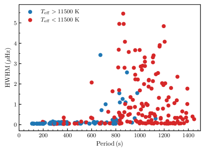
Figure 1: Observed Fourier width versus period for modes in DAVs observed with Kepler and K2. The blue and red points are for modes in stars with $T_{\rm eff}>11$,500 K and $T_{\rm eff}<11$,500 K, respectively.

In this paper we introduce a mechanism that should be present for limiting the growth of mode amplitudes. This mechanism becomes more important at cooler temperatures and might be relevant to the red edge of the DAV instability strip.

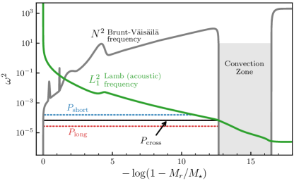
Figure 2: Schematic propagation diagram of a DAV white dwarf. A g-mode with a “short” period would have an outer turning point beneath the convection zone (blue dotted line), while one with a “long” period would have an outer turning point at the convection zone boundary (red dotted line). The crossover point between these two regimes is given by a mode with $P=P_{\rm cross}$ (black horizontal line).

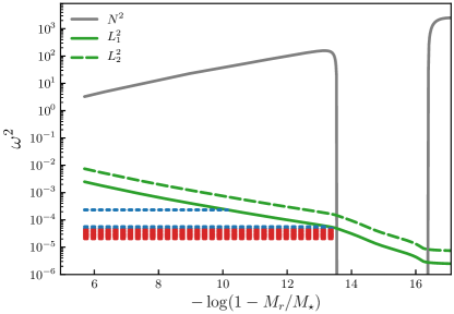
Figure 3: The outer propagation region for a model with the same parameters as EPIC 201806008. The dashed horizontal lines show the region of propagation that the observed modes would have in this model: the blue dashed lines denote modes observed to have $\Gamma<0.3\,\mu$Hz and the red dashed lines modes with $\Gamma>0.3\,\mu$Hz.

3 The Propagation Region

The region of propagation of $g$ modes in a star is defined by the region in which $\omega^{2}<N^{2},L^{2}_{\ell}$, where $\omega=2\pi/P$ is the angular frequency of the mode, $N$ is the Brunt-Väisälä (buoyancy) frequency, and $L_{\ell}$ is the Lamb (acoustic) frequency. In Fig. 2, we show a propagation diagram for a model, computed with MESA (Paxton et al., 2011; Paxton et al., 2013, 2015, 2018). The grey horizontal line denotes the region of propagation of a hypothetical mode whose period, $P_{\rm cross}$, is the minimum required for it to propagate to the base of the convection zone.

In Fig. 3, we show the outer propagation region for a model with the same parameters as EPIC 201806008 ($\log\,g=8.02$, $T_{\rm eff}=10910\,$K). The dashed horizontal lines show the region of propagation that the observed modes would have in this model, where the blue dashed lines denote modes observed to have $\Gamma<0.3\,\mu$Hz and the red dashed lines modes with $\Gamma>0.3\,\mu$Hz. We note that, by setting $\alpha=0.42$ for this model, we can divide the modes into two groups: 1) narrow (blue) modes whose outer turning point is well beneath the convection zone, and 2) wide (red) modes that propagate all the way to the base of the convection zone. In other words, all the modes with $\Gamma>0.3\,\mu$Hz can be explained as propagating to the base of the convection zone, whereas all the modes with $\Gamma<0.3\,\mu$Hz have an outer turning point safely inside this point. Our hypothesis is that the long-period modes, through their interaction with the convection zone, will have systematically larger Fourier mode widths than the short-period modes. In the following sections we examine this statement more quantitatively.

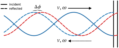
Figure 4: Solid lines: the incoming wave incident on the base of the convection zone (vertical black lines); dashed lines: the waves reflected from the base of the convection zone. The blue curves represent the unperturbed case (reflection from leftmost vertical line) while the red curves show the effect of moving the base of the convection zone to the right (rightmost vertical line). The phase difference of the maxima of the reflected waves in these two cases is labeled as $\Delta\phi$.

4 Asymptotic Theory

We first re-derive a standard result. From Gough (1993) we have that the asymptotic radial wavenumber is given by

$$K^{2}(r)=\frac{\omega^{2}-\omega_{c}^{2}}{c^{2}}-\frac{L^{2}}{r^{2}}\left(1-\frac{N^{2}}{\omega^{2}}\right),$$ (1)

where $N$ is the Brunt-Väisälä frequency, $L^{2}\equiv\ell(\ell+1)$, $c$ is the sound speed, $\omega$ is the angular frequency of the mode, and $\omega_{c}$ is the acoustic cutoff frequency. The group velocity, $v_{\rm gr}$, of gravity waves is given by (see Unno et al., 1989; Gough, 1993)

$$v_{\rm gr} \equiv \frac{\partial\omega}{\partial K}=\left(\frac{\partial K}{\partial\omega}\right)^{-1}$$ (2)

$$= -\frac{1}{\omega K}\left(L^{2}N^{2}/r^{2}\omega^{2}-\omega^{2}/c^{2}\right).$$ (3)

For a mode of overtone number $n$, the time taken for it to propagate from the inner to the outer turning point and back again is $T_{\rm bounce}=n\,P$. Denoting the inner and outer turning points as $r_{1}$ and $r_{2}$, respectively, we find that

$$n\,P=T_{\rm bounce}=2\int_{r_{1}}^{r_{2}}\frac{dr}{|v_{\rm gr}|}.$$ (4)

In the low-frequency, g-mode limit, $K\approx LN/\omega r$, so eqn. 4 can be written as

$$n\pi=\int_{r_{1}}^{r_{2}}Kdr.$$ (5)

This is just the well known quantization condition for asymptotic nonradial modes. Finally, the asymptotic formula for mode periods can be written as

$$P_{n}=\frac{2\pi^{2}n}{\sqrt{\ell(\ell+1)}}\left[\int_{r_{1}}^{r_{2}}\frac{N}{r}dr\right]^{-1}.$$ (6)

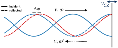
Figure 5: The change in the frequency of the reflected wave ($\omega\rightarrow\omega^{\prime}$) due to the velocity of the base of the convection zone ($v_{CZ}$). This frequency change leads to a change in the radial wavenumber of the wave, leading to a slow accumulation of phase difference as the wave propagates.

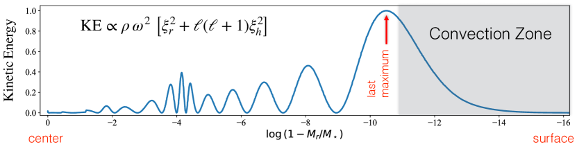
Figure 6: The position of the last maximum of the kinetic energy density (red arrow) before the mode reaches the base of the convection zone. At this point, $v_{\rm gr}$ is finite.

5 Interaction with the
Convection Zone

There are two main ways that a mode’s interaction with the outer convection zone could lead to a loss of its coherence. First, if a mode has a low enough frequency, its outer turning point will be the base of the convection zone. Since the base of the convection zone rises and falls with the surface temperature perturbations of the pulsations, $r_{2}$ in eqn. 6 is time dependent. This leads to variations in $P_{n}$, which in turn lead to an overall lack of coherence of the mode (see Fig. 4). In Montgomery et al. (2015), we showed that the extra phase of the mode, $\Delta\phi$, could be related to the variation in period due to this effect by

$$\Delta\phi_{\rm cav}=2\pi n\left(\frac{\Delta P}{P}\right).$$ (7)

This, in turn, will lead to a damping rate for the mode, as we show in section 7.

A second effect that may play an even larger role is the doppler shift of the wave caused by the motion of the base of the convection zone (see Fig. 5). Formally, this is given by

$$\omega^{\prime}=\omega\,\left(1-v_{CZ}/v_{\rm gr}\right),$$ (8)

where $\omega$ is the frequency of the incident wave, $v_{CZ}$ is the velocity of the base of the convection zone, and $v_{\rm gr}$ is the group velocity of the wave at the base of the convection zone. This frequency difference, as the ray propagates down to the inner turning point and back out to the outer turning point, results in an accumulated phase change of

$$\Delta\phi_{\rm dop} = 2\pi n\,\frac{\Delta\omega}{\omega}$$ (9)

$$= -2\pi n\,\frac{v_{CZ}}{v_{\rm gr}}.$$ (10)

Equation 10 is non-trivial to evaluate since $v_{\rm gr}$ formally goes to zero at the base of the convection zone. However, it is possible to get a finite estimate by looking at its effect on the motion of a well-defined point in the full numerical solution. For example, by using models that differ only in the depth of their convection zones, we can calculate how the position of last maximum of the kinetic energy density (see Fig. 6) changes as a function of convection zone depth. By treating this point as the effective reflecting surface, we can compute its velocity ($v_{CZ}$), which, together with the value of $v_{\rm gr}$ at this point, gives the doppler shift of the reflected wave.

6 Theoretical Damping Rates

For the mode to be completely coherent, it needs to accumulate exactly $2\pi n$ radians of phase each time it propagates back and forth in the star. As shown in the previous section, a changing convection zone can upset this condition, leading to (slightly) destructive interference and a change in amplitude given by

$$\frac{dA}{dt}=-\frac{A}{nP}\left(1-\cos\Delta\phi\right)$$ (11)

(see Montgomery et al., 2015). Assuming that $A\propto e^{-\gamma\,t}$, and averaging $\gamma$ over values of the phase shift from $-\Delta\phi$ to $+\Delta\phi$ gives

$$\gamma=\frac{1}{nP}\left(1-\frac{\sin\Delta\phi}{\Delta\phi}\right).$$ (12)

This is the equation we use to calculate the damping rates of modes given the amplitudes ($\Delta\phi$) of their phase shifts.

7 Results

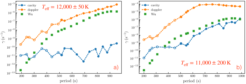
Figure 7: A comparison of the finite-amplitude damping rates for $\ell=1$ modes due to a changing cavity size (blue points, eqn. 7) and those due to doppler shifting of the reflected wave (orange points, eqn. 10). We also show an estimate of the linear growth rate of these modes (green points) based on calculations by Wu (1998) and Wu & Goldreich (1999). Both sets of models have a mass of $0.6\,M_{\odot}$: those in a) have a central $T_{\rm eff}$ of 12,000 K with an assumed pulsation amplitude of 50 K, while those in b) have a central $T_{\rm eff}$ of 11,000 K with an assumed amplitude of 200 K.

Combining eqns. 7 and 10 with eqn. 12, we can compute finite-amplitude damping rates for different pulsation modes. In Figs. 7a,b we show the damping rates for $\ell=1$ modes using two different sets of $0.6\,M_{\odot}$ models. In Fig. 7a, the models have a central $T_{\rm eff}$ of 12,000 K with assumed temperature excursions of $\pm 50$ K; the observed fractional flux amplitude would be approximately $\delta F/F\sim 1$%. The blue points show the damping rate due to the changing size of the g-mode cavity, while the orange points give the damping rate due to the doppler shifting of the reflected wave’s frequency. Fig. 7b is the same but for models with a central $T_{\rm eff}$ of 11,000 K with assumed temperature excursions of $\pm 200$ K; the observed fractional flux amplitude in this case would be $\delta F/F\sim 4$%. The green points in both plots show an estimate of the linear growth rate of these modes based on calculations by Wu (1998) and Wu & Goldreich (1999).

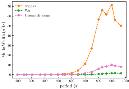
Figure 8: Calculation of mode width assuming that the width is equal to the finite-amplitude damping (“doppler”, orange points) or linear driving (“Wu”, green points) rates. The geometric mean of these two calculations is also shown (magenta points).

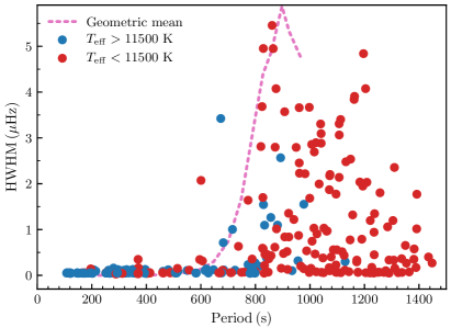
Figure 9: Comparison of the scaled “geometric mean” calculation in Fig. 8 to the observed mode widths of Fig. 1. While suggestive that there might be a connection between the damping effects considered in section 5 and the observed mode widths, further work is needed to establish this conclusively.

The linear growth rates, by definition, do not depend on the amplitude of the pulsations, while the nonlinear damping mechanisms presented here do. First of all, we see that the damping due to the doppler shift of the mode’s frequency is much larger than that due to the variation in the size of its g-mode cavity, for all models and modes. In Fig. 7a, the damping is slightly larger than the driving, indicating that the predicted $T_{\rm eff}$ excursions would be slightly less than $\pm 50$ K. In Fig. 7b, the damping is much larger than the driving, indicating that the predicted $T_{\rm eff}$ excursions should be much smaller than $\pm 200$ K.

Due to the nature of the stochastic excitation mechanism in solar-like pulsators, the theoretical damping rates provide a prediction for the observed Fourier widths of the modes. While this connection is less clear for pulsators with modes that are linearly unstable, we can still compare the calculated damping and driving rates to the observed widths of these modes.

Given this assumption, in Fig. 8 we plot the mode width due to damping from the doppler effect (orange curve and points) and that due to the driving from the Wu and Goldreich convective driving mechanism (green curve and points). For purely phenomenological reasons, we also plot the geometric mean of these two quantities (magenta curve and points).

Finally, in Fig. 9 we plot a scaled version of the geometric mean from Fig. 8 along with the measured mode widths of Hermes et al. (2017). We see that the calculation reproduces the qualitative shape of the envelope of the observed mode widths as a function of period. This suggests that there might be a connection between the damping effects considered in section 5 and the observed mode widths. More work will be needed to establish this relationship more conclusively.

8 Discussion

In the preceding sections we have shown that the modes with observed Fourier widths greater than 0.3 $\mu$Hz have longer periods ($P\gtrsim 800$ s) and are expected to propagate all the way to the base of the surface convection zone in pulsating DA WDs. We have put forward mechanisms through which the convection zone can cause a lack of coherence in these modes. Preliminary results are that this mechanism is stronger at the red edge of the instability strip. However, the size of the effect is such that it may be too large to be consistent with the observed large pulsation amplitudes (a few percent) that are seen in these stars.

An additional effect that is surely present at some level is the overshooting of turbulent fluid motions at the base of the convection zone. These motions will produce an effective turbulent viscosity that will tend to damp the $g$-mode pulsations. This damping, as well as its variation with time, could also lead to a broadening of the modes in frequency space. It is also possible that this overshoot region could at least partially reflect the modes before they have a chance to reach the base of the convection zone. This could reduce the size of the damping due to the doppler shift of the reflected waves that is found in these calculations.

9 Conclusions

In this paper we present a mechanism that could be relevant to the properties of white dwarfs as they cool and approach the red edge of the DAV instability strip. As the convection zone changes its depth during the pulsation cycle, the condition for coherent reflection of the outgoing traveling wave is slightly violated. In effect, this causes the amplitude present in the mode at its linear frequency to slowly spread to nearby frequencies. This decreases the overall amplitude of the mode and leads to damping. This mechanism should be present at some level in all pulsating WDs, and should be larger near the red edge of the DAV instability strip. Preliminary calculations show that this damping is probably too large to be consistent with the observed amplitudes in some DAVs, although other effects may operate which mitigate this. In addition, this mechanism could possibly be relevant for other g-mode pulsators with surface convection zones (e.g., Gamma Doradus stars), or even large-amplitude pulsators such as RR Lyrae stars or high-amplitude Delta Scuti stars (HADs).

References

- Bischoff-Kim et al. (2008) Bischoff-Kim A., Montgomery M. H., Winget D. E., 2008, ApJ, 675, 1512
- Córsico et al. (2012) Córsico A. H., Althaus L. G., Miller Bertolami M. M., Romero A. D., García-Berro E., Isern J., Kepler S. O., 2012, MNRAS, 424, 2792
- Córsico et al. (2016) Córsico A. H., et al., 2016, JCAP, 7, 036
- Gough (1993) Gough D. O., 1993, in Zahn J.-P., Zinn-Justin J., eds, Astrophysical Fluid Dynamics - Les Houches 1987. Elsevier Science Publishers, Amsterdam, pp 399–560
- Hermes et al. (2010) Hermes J. J., Mullally F., Winget D. E., Montgomery M. H., Miller G. F., Ellis J. L., 2010, AIP Conference Proceedings, 1273, 446
- Hermes et al. (2017) Hermes J. J., et al., 2017, ApJS, 232, 23
- Houdek & Dupret (2015) Houdek G., Dupret M.-A., 2015, Living Reviews in Solar Physics, 12, 8
- Isern et al. (2008) Isern J., García-Berro E., Torres S., Catalán S., 2008, ApJ, 682, L109
- Kepler et al. (2005) Kepler S. O., et al., 2005, ApJ, 634, 1311
- Kumar & Goldreich (1989) Kumar P., Goldreich P., 1989, ApJ, 342, 558
- Montgomery et al. (2015) Montgomery M. H., Romero A. D., Córsico A. H., 2015, in Dufour P., Bergeron P., Fontaine G., eds, Astronomical Society of the Pacific Conference Series Vol. 493, 19th European Workshop on White Dwarfs. p. 181
- Mukadam et al. (2006) Mukadam A. S., Montgomery M. H., Winget D. E., Kepler S. O., Clemens J. C., 2006, ApJ, 640, 956
- Mullally et al. (2003) Mullally F., Mukadam A., Winget D. E., Nather R. E., Kepler S. O., 2003, in NATO ASIB Proc. 105: White Dwarfs. p. 337
- Mullally et al. (2008) Mullally F., Winget D. E., Degennaro S., Jeffery E., Thompson S. E., Chandler D., Kepler S. O., 2008, ApJ, 676, 573
- Paxton et al. (2011) Paxton B., Bildsten L., Dotter A., Herwig F., Lesaffre P., Timmes F., 2011, ApJS, 192, 3
- Paxton et al. (2013) Paxton B., et al., 2013, ApJS, 208, 4
- Paxton et al. (2015) Paxton B., et al., 2015, ApJS, 220, 15
- Paxton et al. (2018) Paxton B., et al., 2018, ApJS, 234, 34
- Unno et al. (1989) Unno W., Osaki Y., Ando H., Saio H., Shibahashi H., 1989, Nonradial oscillations of stars. University of Tokyo Press, Tokyo
- Winget et al. (2015) Winget D. E., et al., 2015, in Dufour P., Bergeron P., Fontaine G., eds, Astronomical Society of the Pacific Conference Series Vol. 493, 19th European Workshop on White Dwarfs. p. 285
- Wu (1998) Wu Y., 1998, PhD thesis, California Institute of Technology
- Wu & Goldreich (1999) Wu Y., Goldreich P., 1999, ApJ, 519, 783