A semi-analytical perspective on massive galaxies at $z\sim 0.55$

Abstract

The most massive and luminous galaxies in the Universe serve as powerful probes to study the formation of structure, the assembly of mass, and cosmology. However, their detailed formation and evolution is still barely understood. Here we extract a sample of massive mock galaxies from the semi-analytical model of galaxy formation (SAM) Galacticus from the MultiDark-Galaxies, by replicating the CMASS photometric selection from the SDSS-III Baryon Oscillation Spectroscopic Survey (BOSS). The comparison of the Galacticus CMASS-mock with BOSS-CMASS data allows us to explore different aspects of the massive galaxy population at $0.5<z<0.6$, including the galaxy-halo connection and the galaxy clustering. We find good agreement between our modelled galaxies and observations regarding the galaxy-halo connection, but our CMASS-mock over-estimates the clustering amplitude of the 2-point correlation function, due to a smaller number density compared to BOSS, a lack of blue objects, and a small intrinsic scatter in stellar mass at fixed halo mass of $<0.1$ dex. To alleviate this problem, we construct an alternative mock catalogue mimicking the CMASS colour-magnitude distribution by randomly down-sampling the SAM catalogue. This CMASS-mock reproduces the clustering of CMASS galaxies within 1$\sigma$ and shows some environmental dependency of star formation properties that could be connected to the quenching of star formation and the assembly bias.

1 Introduction

The most luminous and massive galaxies in the Universe serve as powerful probes to study the formation of structure, the assembly of mass and cosmology, but their detailed formation and evolution, especially their connection to feedback processes, quenching of star formation or the assembly bias is still not sufficiently understood or quantified (Tinker et al., 2013; Wechsler & Tinker, 2018). The Sloan Digital Sky Survey SDSS-III/Baryon Oscillation Spectroscopic Survey (BOSS, Schlegel et al., 2009; Eisenstein et al., 2011; Dawson et al., 2013) was dedicated to studying properties of the large-scale distribution of massive galaxies and provides a well studied sample of $\sim 1.5$ million luminous red galaxies (LRGs). The BOSS sample is divided into two: a low redshift (LOWZ) and a high redshift sample (CMASS, stands for “constant mass”), respectively.

The CMASS sample covers a wide redshift range from $0.43<z<0.75$ exhibiting a peak in comoving number density of $n\sim 3.4\times 10^{-4}$ $h^{3}$${{\rm Mpc}^{-3}}$ at $z\sim 0.5$. The stellar mass function evolves very little in this redshift range suggesting that CMASS galaxies are passive and show almost or no on-going star formation (Maraston et al., 2013). A non-evolving sample of massive galaxies provides an excellent “cosmic laboratory” to study galaxy formation and evolution as shown by Bernardi et al. (2016); Montero-Dorta et al. (2016); Montero-Dorta et al. (2017a), and their link to cosmology via e.g. the large-scale structure distribution and clustering of BOSS galaxies studied by Chuang et al. (2016); Rodríguez-Torres et al. (2016); Guo et al. (2018). BOSS LRGs were repeatedly used to determine fundamental cosmological parameters: Cuesta et al. (2016); Gil-Marín et al. (2017); Ross et al. (2017) and to put cosmological models to the test: e.g. Anderson et al. (2014); Beutler et al. (2014); Alam et al. (2017); Sullivan et al. (2017); Mueller et al. (2018). Furthermore, because the sample addresses the most luminous and red galaxies, they act as an important probe to close the gap in understanding the link between dark matter haloes and massive galaxies (Leauthaud et al., 2012; Nuza et al., 2013; Guo et al., 2014; Saito et al., 2016; Favole et al., 2016).

At low redshift LRGs are known to populate the most massive haloes located in denser regions such as the centre of clusters and superclusters (Lietzen et al., 2012). That makes them particularly interesting to study, because they give clues to the assembly of the most massive structures, the formation of haloes, and their connection to their associated galaxies. Thereby the ratio of their stellar to halo masses as a function of halo mass (SHMF) allows for exploring the galaxy-halo connection and the formation and evolution of those galaxies in dark matter haloes of a certain mass range. Or equally, what halo mass is related to a galaxy that produced a certain stellar mass over a certain time. From a more cosmological point of view the relation shows how galaxies trace dark matter and how its density field is distributed. Interestingly, the haloes at intermediate masses produce stars most efficiently, relative to their mass (White & Frenk, 1991; Benson et al., 2003; Bower et al., 2006). It is still barely understood why haloes with lower or higher masses are by orders of magnitudes less efficient (Behroozi et al., 2013). To shed light on this topic one would need to study the full history of mass assembly and star formation within a large redshift range, which is a costly task for “full-physics” hydro-cosmological simulations. The number of particles in question to cover a similar physical volume and amount of galaxies as an observational survey is therefore inaccessible. Different approaches to modelling the population of dark matter haloes with galaxies as well as their formation and evolution inside the haloes, have been developed. One of them being semi-analytical models (hereafter SAMs). SAMs are usually build upon N-body dark matter simulations (e.g Millennium: Springel et al. (2005), MultiDark: Klypin et al. (2016) using merger trees (information of the hierarchical formation of dark matter haloes) and implementing baryonic physics as a post-processing step. For details on semi-analytical modelling we refer to excellent reviews on the field: Baugh (2006); Benson (2010); Baugh (2013); Somerville & Davé (2015); Cora (2016).

SAMs have been used recently in various frameworks to study for example correlation functions and galaxy clustering (Campbell et al., 2015; Farrow et al., 2015; van Daalen et al., 2016), the galaxy-halo connection (Contreras et al., 2013; Contreras et al., 2015); or active galactic nuclei, galaxy mergers, and the cosmic web (Almeida et al., 2008; Liu et al., 2016; Ren et al., 2018; Shirakata et al., 2018). They have been utilised to trace the star formation history (Mutch et al., 2013; Lagos et al., 2014; Orsi et al., 2014; Gruppioni et al., 2015); to understand the galaxy mass-luminosity relations (Zoldan et al., 2018); or the processes regulating star formation (Henriques et al., 2017, 2018; Cora et al., 2018) or generating galaxy colours and metallicities (Yates et al., 2012; Gonzalez-Perez et al., 2014; Rodrigues et al., 2017; Xie et al., 2017; Collacchioni et al., 2018).

Within this paper we connect two major frameworks using a SAM: galaxy clustering and galaxy formation, in order to learn about the nature and properties of those most massive galaxies. Contreras et al. (2013) performed a similar work and claimed that galaxy properties, apart from the stellar mass, e.g., star formation rate or cold gas mass, have more complicated correlation and non-negligible impacts on the clustering. Thereby the type of galaxy (central or satellite) plays a crucial role. Knebe et al. (2018) did a similar study with the MultiDark-SAMs for the SDSS main sample ($z\sim 0.1$). Within our work we expand upon these studies focusing at the redshift $z\sim 0.5$ and CMASS galaxies. For that we use the same publicly available galaxy catalogues called the “MultiDark-Galaxies”. From them we take the SAM-code Galacticus as our modelled galaxy catalogue because it provides proper luminosities in the SDSS $ugriz$-band magnitudes suitable to compare with data from BOSS (Data Release 12), which we adopt as our observational sample.

This paper is organised as the following: In Section 2 we describe the observational and modelled galaxy samples. In Section 3 we show how to replicate the CMASS photometric selection for our model, Galacticus. We further provide confidence plots and a detailed study of various galaxy properties in Section 4. Our results and discussion can be found in Section 5 and Section 6, respectively, and our summary in Section 7. The adopted cosmology in the MultiDark-Galaxies as well as in this paper consists of a flat $\Lambda$CDM model with the following cosmological parameters: $\Omega_{m}=0.307,\Omega_{b}=0.048,\Omega_{\Lambda}=0.693,\sigma_{8}=0.823,n_{s}=0.96$, and a dimensionless Hubble parameter $h=0.678$ (Planck Collaboration et al., 2015). Hereafter, $h$ will is absorbed in the numerical value of its property throughout the text and in all tables and figures.

2 Data Sets and Selection

We use BOSS-CMASS galaxies as our observational and the semi-analytical MDPL2-Galacticus galaxy catalogue product as our modelled data sample. In this section we show the selection algorithms used to generate those samples. We further document all necessary assumptions and corrections applied to the samples in order to create comparable observational and modelled data sets. Those corrections include e.g. adjusting galaxy properties to our chosen cosmology (observations) or generating colours from luminosities (model).

2.1 Observational Data: The BOSS-CMASS Sample

The CMASS-sample was designed to target the most luminous red galaxies in order to produce a uniformly (in mass) distributed samples of galaxies at redshift $0.43<z<0.7$ by applying a set of colour-magnitude cuts Eq. (1)-(8) shown below. The CMASS selection is similar to the algorithms used to target SDSS-I/II Cut-II (Eisenstein et al., 2001) and 2SLAQ LRGs (Cannon et al., 2006), using (g-i) and (r-i) colours to isolate high redshift galaxies, but the algorithm guarantees for an extension towards the bluer colours and the so called “blue-cloud” (BC) galaxies can enter the CMASS-sample. In our study we use BOSS data from Data Release 12 (hereafter BOSS-CMASS DR12; Alam et al., 2015). The following colour-magnitude cuts are used to select the CMASS galaxies:

$$d_{\perp}>0.55,$$ (1)

$$i<19.86+1.6~{}(d_{\perp}-0.8),$$ (2)

$$17.5<i<19.9,$$ (3)

$$r-i<2,$$ (4)

$$i_{\rm fib2}<21.5,$$ (5)

$$i_{\rm psf}-i_{\rm mod}>0.2+0.2~{}(20.0-i_{\rm mod}),$$ (6)

$$z_{\rm psf}-z_{\rm mod}>9.125-0.46~{}z_{\rm mod},$$ (7)

where $d_{\perp}$ is called the “composite colour” with:

$$d_{\perp}=(r-i)-(g-r)/8.0,$$ (8)

$g,r,i$ are the cmodel magnitudes in the AB-system, $i_{\rm mod}$ and $z_{\rm mod}$ refer to model magnitudes, $i_{\rm fib2}$ is the fiber magnitude, and $i_{\rm psf}$ and $z_{\rm psf}$ are the PSF magnitudes. For more information about the set of colour-magnitudes cuts consult the BOSS-CMASS DR12 target selection webpage. Eq. (1) isolates high-redshift objects; Eq. (2) is a sliding magnitude cut that selects the brightest or more massive galaxies with redshift; Eq. (3) defines the faint and bright limits; and Eq. (4) protects from some outliers. Eq. (5) ensures a high redshift measurement success rate; and Eq. (6) and Eq. (7) perform a star-galaxy separation.

We use the latest “Large-Scale Structure (LSS) catalogue” (Reid et al., 2016) from the SDSS Science Archive Server which was cross-matched with the Portsmouth passive galaxy sample to include stellar masses. The stellar masses were generated via a post-processing step using the stellar population models of Maraston (2005) and Maraston et al. (2009) to perform a best-fit to observed ugriz-magnitudes (Fukugita et al., 1996).

We use Planck cosmology and assume a Chabrier (2003) initial mass function (IMF). The Portsmouth galaxy product assumes a WMAP7 flat $\Lambda$CDM cosmology with a dimensionless Hubble parameter of $h=0.7$ (White et al., 2011, same as in the entire BOSS pipeline) and a Kroupa (2001) IMF. Therefore we correct their stellar masses from WMAP7 to Planck cosmology. We further convert the stellar masses to match the assumed IMF of MultiDark-Galaxies models, Chabrier (2003), with the following conversion: ${{\log_{\rm 10}}}M_{\rm Chabrier}={{\log_{\rm 10}}}M_{\rm Kroupa}-0.03925$ (see Table B1 in Lacey et al., 2016).

For the data reduction we use the same approach as Rodríguez-Torres et al. (2016), described in their Sec.2. In order to account for redshift failure and fiber collision we apply weights given by Anderson et al. (2014), using Eq.(9) in Rodríguez-Torres et al. (2016). This results in a total number of 818,817 observed CMASS galaxies (entire redshift range). For this work we select a sub-sample of galaxies in the range $0.5<z<0.6$, which guarantees for maximal completeness in number density (Guo et al., 2018), leaving us with a catalogue of 423,671 galaxies to study. We use this selection to compute the stellar mass function and clustering of the observed galaxies using the Planck parameters as a fiducial cosmology. We also extract the bias and number density from this sample to construct a Halo Abundance Matching (HAM) on the BigMDPL simulation that describes these observations. Furthermore, the BOSS survey covers around $\sim 9,600$ $\rm deg^{2}$ of the sky which corresponds to a volume of $\sim 4.147\times 10^{9}~{}\rm Mpc^{3}$ within our redshift range and assumed cosmology.

2.2 MultiDark-Galaxies: MDPL2-Galacticus

MDPL2-Galacticus is based on the semi-analytical galaxy formation and evolution code Galacticus from Benson (2012) and consists of a large catalogue of galaxy properties including the SDSS $ugriz$-band luminosities. It was run on the 1000$h^{-1}\,{\rm Mpc}$ dark matter simulation MultiDark Planck 2 (hereafter MDPL2: Klypin et al., 2016) following the evolution of $3840^{3}$ dark matter particles with a mass per particle of $m_{p}=2.23\times 10^{9}$ ${\rm{M_{\odot}}}$and minimum 20 particles/halo. Haloes and sub-haloes were identified with Rockstar (Behroozi et al., 2013a) and merger trees constructed with Consistent Trees (Behroozi et al., 2013b). The Galacticus SAM assumes a stellar population synthesis model from Conroy et al. (2009) and a dust model of Ferrara et al. (1999). The definition of the dark matter halo mass is giving by:

$$M_{\rm ref}(<R_{\rm ref})=\Delta_{\rm ref}\rho_{\rm c}\frac{4\pi}{3}R_{\rm ref}^{3},$$ (9)

where $\Delta_{\rm ref}=\Delta_{\rm BN98}$ for $M_{\rm BN98}$ with $\Delta_{\rm BN98}$ being the virial factor as given by the Eq. (6) of Bryan & Norman (1998); $\rho_{\rm c}$ being the critical density of the Universe, and $R_{\rm ref}$ being the corresponding halo radius for which the interior mean density matches the desired value on the right-hand side of Eq. (9). For information on the models’ calibration and intrinsic constrains, we refer to the MultiDark-Galaxies data release paper Knebe et al. (2018, Sec.2.2 and Table 1).

Galacticus returns luminosities, $L$, in the SDSS $ugriz$-bands at the zero-point of the AB-magnitude system in units of $4.4659\times 10^{13}\rm WHz^{-1}$. We apply $M_{AB}=-2.5{{\log_{\rm 10}}}L$, to convert $L$ to absolute magnitudes $M_{AB}$ in each filter band. The filter band was by default blue-shifted to the redshift of the galaxy; meaning that in order to compute the apparent magnitude one must add not only the distance modulus, but also a factor of $-2.5{{\log_{\rm 10}}}(1+z_{0})$ to account for the compression of the photon frequencies at $z_{0}=0.56$. This results in

$$m_{AB}=M_{AB}+DM(z)-2.5{{\log_{\rm 10}}}(1+z_{0}),$$ (10)

with $m_{AB}$ being the observed apparent magnitude in the AB-system and $DM(z)=5{{\log_{\rm 10}}}(D^{z}_{L}/10\rm pc)$ the distance modulus with $D^{z}_{L}$ as luminosity distance at the redshift $z=0.56$ in parsec.

3 Sample Selection and Colour-Magnitude Evaluation

data	sample name	$N_{\rm gal}$	f${}^{\rm total}_{\rm c}$	f${}^{\rm total}_{\rm sats}$	f${}^{\rm sats}_{\rm o}$	$n$ $\times 10^{-4}$	$V_{\rm eff}$$\times 10^{9}$	remark
		total	centrals	total sats	orphan sats	[${{\rm Mpc}^{-3}}$]	[${{\rm Mpc}^{3}}$]
			($N_{\rm gal}$)	($N_{\rm gal}$)	($N_{\rm gal}$)
BOSS-CMASS DR12	CMASS DR12	423,671	$\sim$0.900	$\sim$0.100	-	1.02	4.147	$0.5<z<0.6$
MDPL2-Galacticus	Gal-all	1,844,542	0.794	0.206	0.205	5.737	3.212	entire set of galaxies
			(1,465,070)	(379,472)	(64,478)			${{M_{*}}}>10^{10.7}$ ${\rm{M_{\odot}}}$
MDPL2-Galacticus	Gal-cols	95,683	0.901	0.089	0.112	0.30	3.212	set of colour-magnitude
			(87,167)	(8,516)	(859)			cuts: Eq. (1)-(4)
MDPL2-Galacticus	Gal-dens	314,083	0.848	0.151	0.171	1.02	3.212	red-blue cut using Guo et al. (2013, Eq.7)
			(266,483)	(47,600)	(6,952)			down-sampled with SMF at $z=0.56$
MDPL2-Galacticus	Gal-mass	129,109	0.899	0.101	0.118	0.40	3.212	${{M_{*}}}>10^{11.24}$ ${\rm{M_{\odot}}}$
			(116,120)	(12,989)	(1,373)
(i)	(ii)	(iii)	(iv)	(v)	(vi)	(vii)	(viii)	(ix)

Table 1: The table summarises the properties of the observed and modelled galaxy samples used in our study. Column (i) shows the name of the publicly available galaxy catalogue we extracted a sample form, (ii) gives the label of the corresponding sample throughout this paper, and (iii) its total number of galaxies ${{N_{\rm gal}}}$. The corresponding fraction of central, satellite or orphan galaxies can be found in (iv) f${}^{\rm total}_{\rm c}$ for centrals, (v) f${}^{\rm total}_{\rm sats}$ for all satellites (non-orphans+orphans), and (vi) f${}^{\rm sats}_{\rm o}$ for orphan satellites (the fraction of orphan satellites is calculated with respect to the total number of satellites), respectively. The number density $n$ of each sample and the effective volume $V_{\rm eff}$ can be found in Column (vii) and (viii), respectively. Column (ix) provides comments on the selection. For the observational sample we select BOSS-CMASS DR12 galaxies in the redshift range of $0.5<z<0.6$ and label the sample CMASS DR12. For the modelled galaxies we show the entire galaxies sample above a confidence cut in stellar mass of ${{M_{*}}}>10^{10.7}$ ${\rm{M_{\odot}}}$: Gal-all and the following CMASS-mock samples: Gal-cols, Gal-dens, and Gal-mass at redshift $z=0.56$ (which matches the median redshift of the full CMASS sample). To extract Gal-cols the standard set of CMASS colour-magnitude cuts from Eq. (1)-(4) was applied. For Gal-dens we used a down sampling algorithm shown in Eq. (11) and Eq. (12), where we selected randomly galaxies from the red population that matched the number density of CMASS DR12. For Gal-mass a stellar mass cut at $Mstar>10^{11.24}$ ${\rm{M_{\odot}}}$ was applied according to the findings of Maraston et al. (2013).

In this section we show how we extracted a CMASS-mock sample from the MDPL2-Galacticus catalogue. Since we deal with modelled galaxy properties we only use a limited set of colour-magnitude selection cuts, Eqs. (1)-(4), because the simulation does not distinguish between model and cmodel magnitudes.

In order to test our CMASS-mock samples we compare on the one hand to observed CMASS galaxies from the Portsmouth merged galaxy catalogue of the $12^{th}$ data release (referred to as CMASS DR12) in the redshift range of $0.5<z<0.6$ (the most complete range in terms of stellar masses), which corresponds to a comoving number density of $n=1.02\times 10^{-4}$ ${{\rm Mpc}^{-3}}$at redshift $z\sim 0.55$ in our adopted cosmology. And on the other hand we extract two more CMASS-mock samples aiming at reproducing the colour-magnitude selection by using other galaxy properties as stellar mass. We do that because luminosities or colours are not always available for modelled galaxy samples, especially if they are as large as MDPL2. Furthermore, we can assess the colours and luminosities of our SAM by comparing it with a sample selected by applying a high stellar mass cut. Both methods should produce similar catalogues, because we expect that the most massive galaxies and the brightest and reddest galaxies coincide with each other.

Therefore we create a second and a third CMASS-mock sample by matching the number density and the stellar mass distribution of the observed sample CMASS DR12, or by applying a high stellar mass cut corresponding to CMASS galaxies as reported by Maraston et al. (2013), respectively. We summarise our sample selection in the following list:

• Gal-all: resulting full sample of $\sim 1.8\times 10^{6}$ galaxies after applying a confidence cut in stellar masses: ${{M_{*}}}>10^{9.5}$ ${\rm{M_{\odot}}}$; this is the entire sample of Galacticus at $z=0.56$

• Gal-cols: colour-selected sample; the observational CMASS colour-magnitude selection, Eqs. (1)-(4), described in Section 2.1, has been applied

• Gal-dens: number density-selected sample; the number density of BOSS-CMASS DR12 ($n_{\rm\texttt{CMASS}}=1.02\times 10^{-4}$ ${{\rm Mpc}^{-3}}$) was matched via randomly down-sampling the red population of Gal-all sample stellar mass function (SMF) at $z=0.56$. The red population was selected with a cut in colour as introduced by Guo et al. (2013, Eq.7):

  $$r-i>0.679-0.082~{}(M_{i}-20).$$ (11)

  We use Eq. (11) instead of a simple cut in red-blue separation as $\textit{(g-i)}>2.35$ because otherwise we would exclude a significant amount of galaxies at ${{M_{*}}}\sim 10^{11.2}$ ${\rm{M_{\odot}}}$ and fail to calculate the true stellar mass function. After applying the colour selection, we calculate the fraction between the densities of the stellar mass functions $\Phi$ $\rm dex^{-1}{{{\rm Mpc}^{-3}}}$ of CMASS DR12 and Galacticus and use it to compare to a random distribution, $S_{\rm rand}$, between $[0,1)$:

  $$S_{\rm rand}<\frac{\Phi_{\texttt{CMASS DR12}}}{\Phi_{\textsc{Galacticus}}},$$ (12)

  A galaxy enters the sample if the condition in Eqs. (11) is fulfilled, otherwise it is discarded.

• Gal-mass: stellar mass-selected sample; we apply a stellar mass ${{M_{*}}}>10^{11.24}$ ${\rm{M_{\odot}}}$ on Gal-all (see Maraston et al. 2013)

In Table 1 we summarise the properties of our observational and modelled CMASS samples. We show the total number of galaxies $N_{\rm gal}$, total numbers and fractions of “centrals”, “satellites”, and “orphan (satellites)”, number densities $n$, and effective volumes $V_{\rm eff}$. Although the $N_{\rm gal}$ and $n$ are different in each CMASS-mock sample, the fraction of centrals (f${}^{\rm total}_{\rm c}\sim 0.9$) and satellites (f${}^{\rm total}_{\rm sats}\sim 0.1$) are almost identical and agree perfectly with the observation (Guo et al., 2014; Rodríguez-Torres et al., 2016). However, we note that the number density of the Gal-cols sample $n_{\rm\textsc{Galacticus}}=0.30\times 10^{-4}$ ${{\rm Mpc}^{-3}}$ roughly corresponds to only 1/3 of the BOSS-CMASS DR12 with $\sim 1.02\times 10^{-4}$ ${{\rm Mpc}^{-3}}$. The discrepancy in the numbers and its consequences will be discussed later. In the following section we perform sanity checks on our Gal-cols CMASS-mock by directly comparing with BOSS-CMASS DR12 data. Note that to avoid crowding we only show Gal-cols and the observational sample in the figures.

3.1 Gal-cols: The Composite Colour $d_{\perp}$

Figure 1: Colour-Magnitude diagram for the modelled sample Gal-cols (filled coloured contours) at $z=0.56$ and BOSS-CMASS DR12 galaxies in the range of $0.5<z<0.6$ (red dashed contours) for observed frame $d_{\perp}$ colour compared to observed apparent $i$-band magnitudes $m_{\rm AB_{i}}$. The solid black polygon-shaped area represents the CMASS colour-magnitudes cuts, the grey hexagons represent the total population of galaxies, Gal-all. Modelled and observed galaxies are in very good agreement with each other.

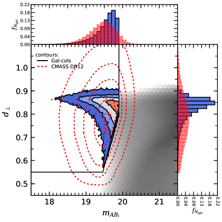
The composite colour $d_{\perp}$ is a colour combination defined in Eq. (8) and the key colour selection parameter for CMASS galaxies involving three bands: g,i, and r. Fig. 1 presents the colour-magnitude diagram (CMD) where $d_{\perp}$ is shown compared to the observed i-band magnitudes, $m_{\rm AB_{i}}$. This is the first and most important sanity check we use to assess our colour selection. The CMASS colour-magnitude selection described in Eq. (1) and Eq. (3) are shown as a polygon-shaped area with a thin solid black line, where all galaxies within this area enter the selection. The Galacticus CMASS sample, Gal-cols, is shown in black filled coloured contours and BOSS-CMASS DR12 in red dashed empty contours. We show the parameter space of the entire set of galaxies, Gal-all, as grey logarithmic binned hexagons in the background to point out that the CMASS sample is only a tiny fraction of the total set of galaxies that Galacticus provides. For the contour-figures we use throughout this work the following confidence levels in per cent: [2.1, 13.6, 31.74, 68.26, 95, 99.7].

The histogram panels on the top and on the right hand side give information about the distribution of galaxies along the binned axes using 40 bins normalised by the total number of galaxies of each sample. The histograms show the same colour and line style keys as the contours: black solid lines and blue filled bars for Galacticus Gal-cols sample and red dashed lines and empty bars for BOSS-CMASS DR12. The histogram of Gal-all is not shown for reasons of over-crowding.

While the majority of the modelled galaxies lies outside the CMASS selection, we nevertheless report that a substantial number enter it. Their numbers can be found in Table 1 under the label Gal-cols. We like to remark that Maraston et al. (2013, Fig.17) report similar results for their adopted SAM. One can see in the histogram panels that Galacticus’ number of galaxies in each bin is in general higher and less spread across the axes compared to the observations. In the next section we will discuss this issue in form of a colour-colour diagram in more detail.

3.2 Gal-cols: Colour-colour and Colour-mass Diagrams

Figure 2: Top: Colour-colour diagram for observed colours (r-i) vs. (g-i) for Gal-cols (filled coloured contours) and CMASS DR12 (red dashed contours). The horizontal thin solid black line represents the $d_{\perp}$-cut and the vertical thin solid black line the red-blue separation of $\textit{(g-i)}=2.35$. The filled yellow circles show modelled RS of different i-band magnitude slices from Montero-Dorta et al. (2016). Bottom: Observed frame colour separation (g-i) vs. $M_{*}$.

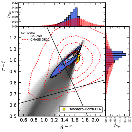
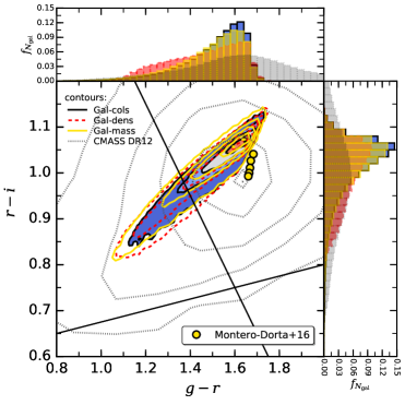
We show in the upper panel of Fig. 2, the (r-i) vs. (g-i) colour-colour diagram. The observed CMASS data (referred to as CMASS DR12) extends over a much larger region in the (r-i) and (g-i) than Galacticus Gal-cols. This is most likely due to the fact that uncertainties (i.e., photometric errors) are not implemented in the model, so no artificial blurring was produced compared to the observations. We also note that the centroid of the Gal-cols distribution is located at slightly redder colours ($\textit{(r-i)}\sim 1.05$ and $\textit{(g-i)}\sim 1.7$) than those of the observations and the location of the intrinsic “red sequence” (RS) from Montero-Dorta et al. (2016). The intrinsic RS is the a narrow sequence of massive red galaxies modelled as an extended Gaussian and is constituted as the counterpart to the “blue cloud” which is a more heterogenous population consisting of galaxies with bluer colours Montero-Dorta et al. (2016). We further include the composite colour $d_{\perp}$-cut as a horizontal; and a common separation of red and blue galaxies, $\textit{(g-i)}=2.35$ (Masters et al., 2011), as a vertical thin solid black line.

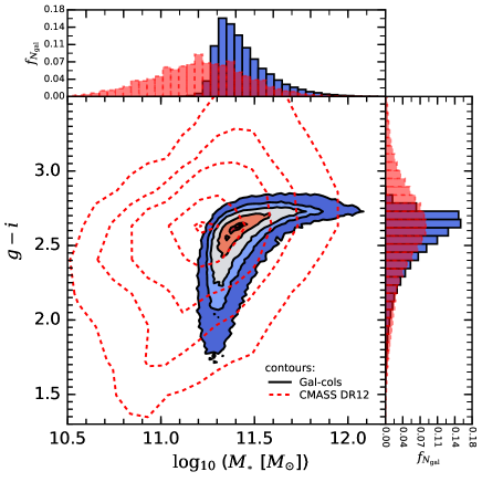
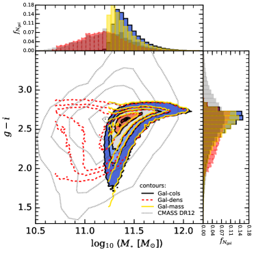
We show in the lower panel of Fig. 2 the (g-i) colour dependence on stellar mass. The Gal-cols’ galaxies are slightly more massive (0.2 dex) than their observational counterparts from the Portsmouth merged catalogue, but the samples are in very good agreement.

4 Sample Comparison

Since luminosities are due to many uncertainties involved in the SPS fitting (see e.g. Conroy et al. 2009) much more complicated to model than masses, SAMs often reproduce only SMFs to a certain degree. Observations need to go the other way: fluxes have been measured and stellar SED fitting performed to assume stellar masses (Maraston et al., 2006). Usually a huge computational effort was brought forward to create luminosities for SAMs applied to volumes as large as MultiDark. Therefore we want to investigate the variation in our samples of selecting CMASS galaxies by colour (as done in observations) vs. by other galaxy properties as stellar mass (as mentioned in the previous section), using the fiducial plots from Section 3 once again.

Colour-Magnitude diagram (CMD):

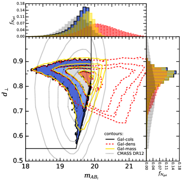
Fig. 3 presents in the upper panel the CMD (as in Fig. 1) for the three modelled samples comparing observed frame $d_{\perp}$ colours to observed $i$-band magnitudes, $m_{\rm AB_{i}}$. A large part of the galaxies of the Gal-dens sample and Gal-mass sample lie outside the polygon reflecting the colour selection.The peak in magnitudes of Gal-dens is shifted 0.3 mags to fainter luminosities compared to Gal-cols and extending into the low-luminosity regime. Gal-mass agrees pretty well with Gal-cols, where its peak is located exactly on the CMASS edge with $m_{\rm AB_{i}}=19.9$.

Colour-colour diagram:

In the middle panel of Fig. 3 we show the colour-colour diagram for observed colours (r-i) vs. (g-i) (as in Fig. 2 lower panel). The horizontal black line represents the $d_{\perp}$-cut and the vertical black line the red-blue separation of $\textit{(g-i)}=2.35$. The filled yellow circles show modelled RS of different $i$-band magnitude slices from Montero-Dorta et al. (2016). The three samples are in very good agreement with each others, but we can see that the galaxies of Gal-dens and Gal-mass extend slightly toward “bluer” colours.

Colour-mass diagram:

In the lower panel of Fig. 3 we show observed frame colour (g-i) vs. $M_{*}$ (as in Fig. 2, lower panel). This figure shows that the mass distribution of the three samples is quite different. Gal-dens, which has the same number density as BOSS, does not coincide with the sample selected by colour, Gal-cols. However, the galaxies of the Gal-dens sample can be bound within the contours of BOSS-CMASS DR12. Alternatively, a high-mass cut in stellar mass can be used to mimic the Gal-cols sufficiently. The next paragraph is dedicated to studying the distribution of stellar masses in our samples in more detail.

Figure 3: Fiducial plots discussed in Section 3 including all three CMASS-mocks of Galacticus at redshift $z=0.56$: Gal-cols (filled coloured contours), Gal-dens (red dashed contours), and Gal-mass (yellow solid contours) compared to CMASS DR12 (dotted-dashed grey contours) within the range $0.5<z<0.6$. Top: CMD. The solid black polygon-shaped area represents the CMASS colour-magnitude selection. Middle: observed colour (r-i) vs (g-i). The horizontal black line represents the $d_{\perp}$-cut and the vertical black line in the same panel the red-blue separation of $\textit{(g-i)}=2.35$. The filled yellow circles represent the modelled RS of different $i$-band magnitude slices from Montero-Dorta et al. (2016). Bottom: (g-i) vs. $M_{*}$.

Stellar mass function:

In Fig. 4 we present the stellar mass functions (SMFs) at redshift $z=0.56$ for the total number of model galaxies from Galacticus Gal-all sample, as well as the CMASS-mocks: Gal-cols, Gal-mass, and Gal-dens compared to CMASS DR12 (filled yellow circles). We state errors in the y-axis of the density functions as $\sigma_{\rm i}=\frac{y_{\rm i}}{\sqrt{N}_{\rm i}}$, where $\rm i=0...n_{\rm bins}$, $y_{i}$ stands for the data on the y-axis, $N_{\rm i}$ for the number of galaxies in each bin, and $n_{\rm bins}$ for the number of bins.

Figure 4: Galacticus’ stellar mass functions for the entire sample of galaxies (thin black line) and CMASS-mock samples: Gal-cols- (blue solid line), Gal-dens (red dashed line), and Gal-mass (grey dotted-dashed line) at redshift $z=0.56$ compared to CMASS DR12 Portsmouth merged catalogue (filled yellow circles) in the range of $0.5<z<0.6$. Their errors bars are located within the size of the markers. In order to improve the readability of the figure, we removed the vertical line dropping to zero at ${{M_{*}}}>10^{11.24}$ ${\rm{M_{\odot}}}$ due to the stellar mass cut applied on Gal-mass.

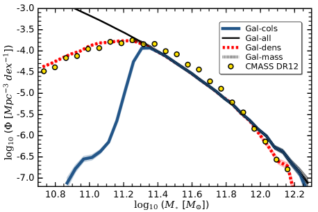
As expected, the different CMASS-mock samples of Galacticus agree very well with each others. They show only slight variation at the high-mass end compared to Gal-cols, due to the colour selection which excludes a few bright . Those could enter in Gal-dens and Gal-mass because no colour selection was performed. At intermediate masses all three samples agree perfectly with each other, but their abundances lie slight beyond the observations. At lower masses we report that the Gal-cols sample shows the same typical shape of incompleteness in the stellar mass function as e.g. Rodríguez-Torres et al. (2016, Fig.3) for the BigMultiDark BOSS light-cone (BigMD-LC) or Maraston et al. (2013).

In summary we have shown that using a simple cut in stellar masses provides a good approximation for the observed CMASS sample. A number density sample (created with a down-sampling algorithm) draws the SMF of CMASS perfectly, but permits bluer and low-mass objects to enter the sample. Those objects have fainter $i$-band magnitudes than CMASS as seen in Fig. 3 upper panel. However, their colours and stellar masses are still in agreement with CMASS as shown in the middle and lower panel of Fig. 3. In the following sections we will come back to the question if a CMASS-mock can be selected by other properties than colours and magnitudes and assess if a colour selections provides a more valid sample that a simple cut in stellar mass particularly for our SAM. Addressing a fully red population is crucial if one once to study CMASS galaxies, therefore we study the “red sequence” (RS) population and its $i$-band luminosity in the next paragraph.

Luminosity function:

Figure 5: Luminosity functions for Galacticus’ CMASS-mock samples: Gal-cols (blue solid line), Gal-dens (red dashed line), and Gal-mass (grey dotted-dashed line) compared to the “red sequence” best-fit Schechter-function from Montero-Dorta et al. (2016, Table 3 & Fig.14) (thin grey dashed line) at redshift $z=0.555$. The errors of BOSS-CMASS DR12 are shown within the size of the markers.

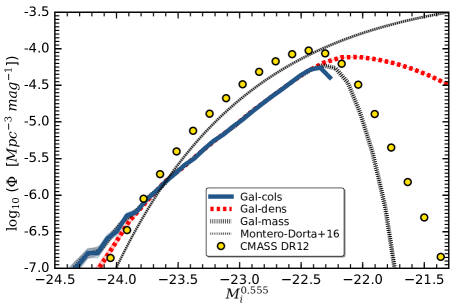
In Section 3.2 we briefly mentioned the “red sequence” (RS) population of CMASS galaxies. Now we want to discuss this topic in more detail and investigate if Galacticus’ CMASS-mock galaxies also exhibit such a population. The RS can be found in observations as a sort of irregular blob in the (r-i) vs. (g-i) parameter space, elongated across the (g-i)-axis due to the $g$-band magnitudes higher error sensitivity. Montero-Dorta et al. (2016) developed an analytic method to model the RS luminosity function (LF) and constrained Schechter-fit parameters. We mimic Galacticus’ RS-samples by selecting red galaxies by applying Eq. (11) to Gal-cols, Gal-dens, and Gal-mass, respectively. In Fig. 5 we compare Galacticus’ CMASS-mock samples to the best-fit of Montero-Dorta et al. (2016) at $z=0.555$. The CMASS-mocks were further blue-shifted to the same redshift using an approximated K-correction of $-2.5{{\log_{\rm 10}}}(1+z)$ (Blanton & Roweis, 2007) to fit the redshift of the Schechter-function.

We report that the reddest galaxies of Galacticus exceed the LF of the observations and the Schechter-fit of about 0.40 and 0.25 mags, respectively, at the bright end. At the faint end all three CMASS-mock samples poorly reproduce the Schechter-fit and their LF can roughly be estimated by a power law. We note that due to the cut in $i$-band magnitude (see Eq. (3)) Gal-cols’s LF is abruptly cut off at $M_{\rm AB}\sim-22.2$.

5 Results

In this section we present our results for the CMASS-mock samples Gal-cols, Gal-mass, and Gal-dens of Galacticus. We show stellar to halo mass ratios as a function of halo mass (SHMFs), halo occupation distributions (HODs), and projected 2-point correlation functions (2pCFs).

5.1 Galaxy-Halo Connection

The Galacticus model assumes virial over-densities to define halo masses, but the measurements we want to compare to use $\Delta_{c}=200$, where $c$ refers to the critical over-density. Therefore we convert the halo masses $M_{\rm vir}$ of our samples to the halo mass of our references $M_{\rm 200c}$ following Łokas & Mamon (2001, Sec. 2.1). Particularly, we use their Eq. (8) to calculate the ratio of the halo masses $P_{{{M_{\rm Halo}}}}={{M_{\rm 200c}}}/{{M_{\rm vir}}}$ which depends on the halo concentration parameter ${{C_{\rm NFW}}}$ as defined by Navarro-Frenk-White (NFW, Navarro et al., 1997). Since the Galacticus model does not provide this quantity nor the virial radius as outputs, we have to estimate the values using the fitting-formula of Klypin et al. (2016, Eq.(24)) and the corresponding values in Table 2 for $z=0.50$. We calculate the $P_{{{M_{\rm Halo}}}}$ for each galaxy separately, however the median over all ratios is $P_{{{M_{\rm Halo}}}}\sim 0.884\pm 0.002$. Our estimated NFW concentration parameters can be found roughly in the range of $4\mathrel{\hbox{\hbox to0.0pt{\hbox{\lower 4.0pt\hbox{$\sim$}}\hss}\hbox{$<$}}}{{{{C_{\rm NFW}}}}}\mathrel{\hbox{\hbox to0.0pt{\hbox{\lower 4.0pt\hbox{$\sim$}}\hss}\hbox{$<$}}}6$ for $10^{13.3}<{{M_{\rm 200c}}}<10^{15.3}$ ${\rm{M_{\odot}}}$.

Note further that we refer to a “central halo” as the top-level dark matter halo in a certain merger tree and to “central galaxies” or “centrals” as the galaxies which reside in the centre of that haloes. From hereafter we exclude all orphan satellites because in the Galacticus model they are not connected to the current central halo anymore, but point to the dark matter halo they belonged to in the past (see Knebe et al. 2018, A2 for clarification). Furthermore, their positions are not traced in the Galacticus model, but are assigned to the central galaxies they have been associated to previously. This introduces uncertainties when calculating correlation functions which we avoid by excluding them.

Figure 6: Top: SHMF of central galaxies of Galacticus’ CMASS-mock samples: Gal-cols (blue solid line), Gal-dens (red dashed line), and Gal-mass (grey dotted-dashed line). They are in excellent agreement with BigMD-LC with in $0.5<z<0.6$ (filled yellow circles), various HAMs realisations at $z\sim 0.55$ (shown as a thin green line) from Behroozi et al. (2013), and weak-lensing observation from CFHT Stripe 82 ($0.4<z<0.6$) from Shan et al. (2017) (shaded yellow area). The additional right y-axis represent the estimated halo concentration parameter ${{C_{\rm NFW}}}$ for Gal-cols and Gal-dens, respectively. Middle and Bottom: Stellar masses, $M_{*}$, and values for the intrinsic scatter, ${{\sigma_{\log_{\rm 10}{{M_{*}}}}}}$, respectively, as a function of $M_{\rm 200c}$ for the same samples as shown in the top panel.

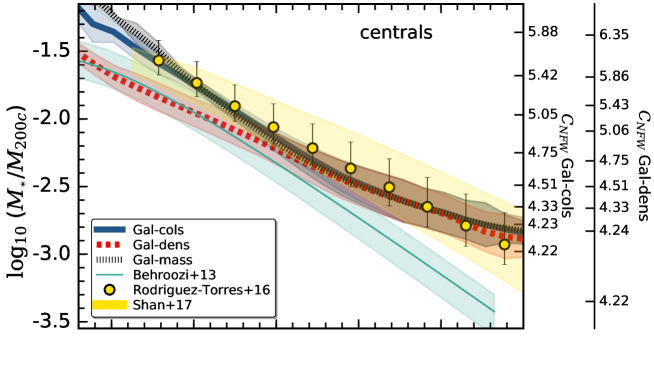
Stellar to halo mass ratio $M_{*}$/$M_{\rm 200c}$:

In the upper panel of Fig. 6, we show SHMF of our CMASS-mocks for central galaxies only (hereafter “centrals”) compared to the halo abundance matching (HAM) model from Rodríguez-Torres et al. (2016) based on the BigMultiDark simulation box with 2.5$h^{-1}$Gpc side-length and clustering results from BOSS-CMASS light cone (BigMD-LC, a mock light cone constructed with the sub-halo abundance matching modelling technique (sHAM) which reproduces BOSS-CMASS DR12 Large Scale Structure catalogue perfectly) within $0.5<z<0.6$. We further compare our SAM data to a compilation of various HAM realisations from Behroozi et al. (2013) at $z\sim 0.55$ and weak-lensing measurements from the Canada-France-Hawaii Telescope (CFHT) Stripe 82 from Shan et al. (2017) within $0.4<z<0.6$, respectively. The additional y-axis on the right represents the estimated values for the NFW profile halo concentration, ${{C_{\rm NFW}}}$, for the two mock samples, Gal-cols and Gal-dens, respectively. Note that we do not show an additional right axis for Gal-mass because its values are similar to Gal-cols. We report that our CMASS-mocks are in very good agreement with both, BigMD-LC and weak-lensing results e.g. Gal-cols and Gal-mass coincide with the data from the BigMD-LC to a high degree. However, Gal-dens agrees best with the HAM at low halo masses but then coincide with the other two samples at ${{M_{\rm 200c}}}\sim 10^{13.5}$. In general we expect Galacticus’ samples not to follow the HAM from Behroozi et al. (2013) because they use very different SMF to build up their model (PRIMUS and GALEX Moustakas et al. 2013). Their SMF predicts less massive objects than those from BOSS as we also found for Gal-dens sample.

Additionally, we tested the impact on the results using Galacticus native definition of over-densities ($\Delta_{\rm BN98}$) and their corresponding halo mass $M_{\rm BN98}$. The impact on the SHMF is small but visible on most massive haloes, but within the error estimations.

Star formation efficiency:

In the middle panel of Fig. 6 we plot the corresponding $M_{*}$ at fixed halo mass and show that the stellar masses truly stays constant for increasing halo masses up to ${{M_{\rm Halo}}}\sim 10^{13.5}~{}{{{\rm{M_{\odot}}}}}$ considering Gal-cols and Gal-mass. Then $M_{*}$ increases continuously which explains the shallower slope of the SHMF in the high-mass regime. That means that the most massive haloes in the CMASS-mocks host galaxies which have been producing stars more efficiently in their lifetime compared to the BigMD-LC or the HAM.

Intrinsic scatter ${{\sigma_{\log_{\rm 10}{{M_{*}}}}}}$:

In the lower panel of Fig. 6 we plot the intrinsic scatter between stellar and halo mass, ${{\sigma_{\log_{\rm 10}{{M_{*}}}}}}$, for Galacticus CMASS-mock samples. As reported in the literature (e.g. Moster et al., 2010; More et al., 2011; Leauthaud et al., 2011; Tinker et al., 2017), the relation between the stellar and halo mass is not one-to-one, meaning that the most massive haloes do not host the most massive galaxies (as requested by e.g. HAM models). Furthermore, two haloes with the same mass can host different galaxies with different stellar masses due to distinct assembly history, environmental effects, or feedback mechanisms (to name only a few). The distribution in stellar mass at fixed halo mass is called “intrinsic (log-normal) scatter” and is given by the standard deviation of logarithmic base 10 stellar mass at that halo mass (Tinker et al., 2013). As shown in the lower panel of Fig. 6, ${{\sigma_{\log_{\rm 10}{{M_{*}}}}}}$ varies from sample to sample. It depends strongly on halo mass for Gal-cols and Gal-mass and drops to a minimum at ${{M_{\rm 200c}}}\sim 10^{13}$ ${\rm{M_{\odot}}}$. This means that for growing halo mass, the stellar mass of galaxies residing in these haloes stays constant until the halo reaches a certain mass threshold. Gal-dens does not exhibit such a threshold or minimum, but shows an almost constant scatter of ${{{{\sigma_{\rm{log}{{M_{*}}}}}}}}\sim 0.15$ dex for haloes with masses of ${{M_{\rm 200c}}}>10^{14}$ ${\rm{M_{\odot}}}$ and then declines smoothly to ${{{{\sigma_{\rm{log}{{M_{*}}}}}}}}=0.09$ dex for ${{M_{\rm 200c}}}<10^{14}$ ${\rm{M_{\odot}}}$. Due to the down-sampling process on the SMF of BOSS, Gal-dens exhibits a higher fraction of low-mass haloes than the other CMASS-mocks which is reflected in the intrinsic scatter.

Halo occupation distribution (HOD):

Figure 7: Halo occupation distributions split into their components where solid lines represent centrals+satellite galaxies (short: centrals+sats), long dashed lines represent centrals and short dashed lines satellites only. Galacticus’ samples are shown as thick blue lines in the panels from left to right: Gal-cols, Gal-dens, and Gal-mass. We compare to the HOD model from Reid et al. (2014) (thin red lines) and to the BigMD-LC based on abundance matching from Rodríguez-Torres et al. (2016) (yellow filled circles on black thin lines) using the same line style keys as Galacticus for their HOD components. <$N_{\rm gal}$> is the mean number of galaxies of a halo with a certain mass $M_{\rm 200c}$.

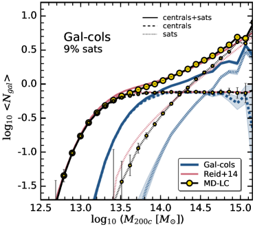
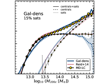
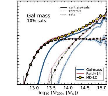
As a second tool to describe galaxy-halo connection, we present the HOD, the mean number of galaxies per halo, <$N_{\rm gal}$>, as a function of the halo mass, $M_{\rm 200c}$. The contribution to the form of the HOD can be divided into central galaxies, modelled as a step function, and satellites, following a power law (Berlind et al., 2003; Zheng et al., 2005). In Fig. 7 we show in three panels the HOD components for our CMASS-mocks from left to right: Gal-cols, Gal-dens, and Gal-mass.

Furthermore, we compare to a HOD-fit from $N$-body simulations constructed from SDSS-III DR10 data Reid et al. (2014, their MedRes0 simulation box) modified to the number density of CMASS at $z=0.56$ (by applying a factor of $1/1.31$ to their HOD in order to correct from their adopted number density to $n=1.02\times 10^{-4}$ ${{\rm Mpc}^{-3}}$). We use their best-fitting model from an adaptation of Zheng et al. (2005). We further compare to the first MDPL cosmological simulation. This simulation uses the same cosmology and parameters as MDPL2, like 1$h^{-1}$Gpc side-length of the box and we constructed the HODs by applying the same HAM-recipe as described in Rodríguez-Torres et al. (2016) for the BigMDPL.

All Galacticus CMASS-mock samples show highly diverse shapes of their HODs where the Gal-dens follows our adopted references best. In the high-mass end and for the contribution of satellites, Gal-dens agrees with the observations better than the other two. Although Gal-cols and Gal-mass show abundances of satellites in agreement with observations ($\sim 10$%, see Table 1), Gal-dens is with 15% satellites the only sample where the HOD of satellites is comparable to the data.

The “knees” of the HOD differ a lot between the CMASS-mock sample being estimated by eyeballing: ${{M_{\rm Halo}}}\sim 10^{13.7}$ ${\rm{M_{\odot}}}$ for Gal-cols and ${{M_{\rm Halo}}}\sim 10^{13.5}$ ${\rm{M_{\odot}}}$ for Gal-dens and Gal-mass, respectively, and to the observation with ${{{{M_{\rm min}}}}}=10^{13.180}$ ${\rm{M_{\odot}}}$. The transition between a halo hosting zero to at least one galaxy is more gradually for Gal-dens and more steep for Gal-cols and Gal-mass. The halo mass where a halo cannot host at least one satellite anymore (see short dashed line) varies from ${{M_{\rm Halo}}}\sim 10^{13.3}$ ${\rm{M_{\odot}}}$ (Gal-dens) to ${{M_{\rm Halo}}}\sim 10^{13.8}$ ${\rm{M_{\odot}}}$ (Gal-cols) and corresponds to ${{{{M_{\rm cut}}}}}=10^{13.328}$ ${\rm{M_{\odot}}}$ for the observations and BigMD-LC, respectively.

All CMASS-mock samples show a similar $M_{\rm 200c}$ $M_{1}$ between $10^{14.3}<{{M_{\rm 200c}}}<10^{14.7}$ ${\rm{M_{\odot}}}$ compared to the data with ${{M_{\rm 200c}}}\sim 10^{14.2}$ ${\rm{M_{\odot}}}$. A large plateau also corresponds to large $M_{1}/M_{min}$-ratio being $\sim 10$ for Gal-cols and Gal-mass and $\sim 6$ for Gal-dens, compared to our references with $\sim 11$. This ratio has a significant impact on the shape of the correlation function (Benson et al., 2000) meaning that galaxies within a wide range of mass or luminosity exhibit a power-law correlation functions (Zheng et al., 2005).

The HODs for centrals (blue thick dashed lines) show incompleteness at the highest halo mass for all Galacticus CMASS-mocks, mainly due to the limited volume of the simulation box. We also see that the Gal-dens CMASS-mocks lacks significantly in high-mass central galaxies which have been excluded during the down-sampling procedure. However, the abundance of the satellites are in complete agreement with our references. Furthermore, the fact that Gal-cols and Gal-mass show a smaller scatter in stellar mass than Gal-dens can be directly read from the HODs of the satellites.

5.2 2-point Correlation Function (2pCF)

Figure 8: The projected 2-point correlation function for Galacticus CMASS-mock samples: Gal-cols (blue solid line), Gal-dens (red dashed line), and Gal-mass (grey dotted-dashed line) at redshift $z=0.56$ compared to the BigMD-LC (filled yellow circles) for centrals+sats (left) and centrals only (right). The amplitude and shape of the 2pCF is highly diverse for our different CMASS-mock samples and also depends on the galaxy type. The best reproduction of the observations was achieved in general by the Gal-cols sample.

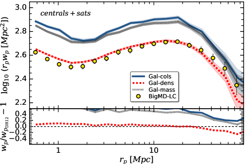
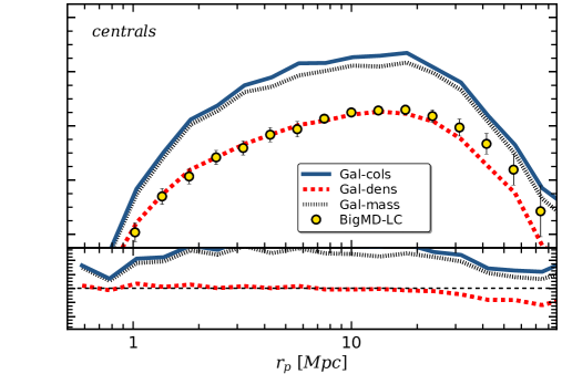
In this section we present our results for the projected 2-point correlation function (2pCF) for our CMASS-mock samples. We use the corrfunc software package from Sinha (2016) and the standard Landy & Szalay (1993) estimator to calculate the functions. We produce 2pCFs with 20 log-spaced bins in the range of $0.5<{{{{r_{\rm p}}}}}<150$ ${\rm Mpc}$ with an integration length of ${{{{\pi_{\rm max}}}}}=150$ ${\rm Mpc}$. We also show the influence of the galaxy type by calculating correlation functions for central and satellite galaxies (short: centrals+sats) and centrals only.

2pCFs for different galaxy types:

In Fig. 8 we present 2pCFs for centrals and satellite galaxies (left) and centrals only (right). We compare to the BigMD-LC within $0.5<z<0.6$, using the same data and treatment as described in Rodríguez-Torres et al. (2016, Sec 5.1.). We estimate the uncertainties of our CMASS-mocks for centrals and satellites using 200 realisations of the MD-Patchy mocks Kitaura et al. (2016). In order to account for the smaller box size-length of MDPL2 we used the MD-Patchy mocks down-scaled to 1$h^{-1}$Gpc. We note that, we did not construct error bars for centrals only because the MD-Patchy code does not distinguish between central and satellites.

In the lower panel of Fig. 8, we show the residuals for Galacticus CMASS-mock samples compared to the BigMD-LC. The CMASS-mocks Gal-cols and Gal-mass fail to reproduce the 2pCF of the BigMD-LC, independently if considering centrals and satellite galaxies together or centrals only. However, the shape of their functions are similar but they exhibit a constant shift of $\sim 0.5$ dex towards higher amplitudes compared to BigMD-LC. Only Gal-dens is in very good agreement with the data over a large range of ${{r_{\rm p}}}$ for both, centrals and satellites and centrals only.

If we include low-mass objects as in the Gal-dens sample the clustering amplitude is reduced at all scales except of the largest with ${{{{r_{\rm p}}}}}>40~{}\rm Mpc$ in full agreement with the results of the the HODs in Fig. 7. The left panel of that figure shows that low-mass halos are underrepresented in the Gal-cols’ HODs resulting in a higher amplitude of the correlation functions in Fig. 8, because only the distances between the most massive objects have been taken into account. Gal-dens’ HOD (middle panel) and 2pCF agree well with both, MD-LC in Fig. 7 and BigMD-LC in Fig. 8, because more low-mass objects could enter the sample. This is true for centrals and satellite galaxies or for centrals only. We therefore investigate which galaxies contribute the most to the correlation function by selecting subsamples for different subsequent stellar mass cuts. We further hereafter drop the discussion of the Gal-mass sample because the results from it is almost identical to that from the Gal-cols sample.

2pCFs of various subsequent $M_{*}$ cuts:

Figure 9: Projected 2-point correlation functions of sub-samples of Galacticus’ CMASS-mock Gal-dens (solid lines) using the subsequent $M_{*}$ cuts (indicated by the keys) compared to BOSS-CMASS DR12 (markers).

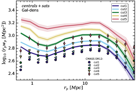
We show the 2pCFs of sub-samples of the CMASS-mock sample Gal-dens in Fig. 9. The sub-samples were constructed by the applying a subsequent stellar masses cuts in $\log_{\rm 10}$($M_{*}$ $[{{{\rm{M_{\odot}}}}}]$): (cut1) 11.21, (cut2) 11.31, (cut3) 11.41, (cut4) 11.51, and (cut5) 11.61. We use again 200 realisations of the MD-Patchy mocks for the estimation of the uncertainties as in Fig. 8. Note that we only present results for Gal-dens because only this sample provides a sufficient number density of galaxies. We can see in the figure that, modelled and observed galaxies are in poor agreement with each other. In order to improve the clustering we tried to fix the number density $n$ of Galacticus’ sub-samples in order to match those of BOSS-CMASS DR12. This experiment only improved the 2pCF slightly.

6 Discussion

Before we discuss our results we want to add a few notes about the influence of Galacticus native tuning and model configuration. Most importantly, Galacticus has not been specifically calibrated on MDPL2, but its most favorables parameter set and configuration were used. Although Galacticus was tuned to match the $K,b_{j}$-band luminosity functions at $z=0$ and the local colour-magnitude diagram at $z=0.1$, its luminosities and colours do not perfectly match the CMASS galaxy properties. Therefore, we examine if alternative approaches to select a CMASS-mock (e.g. a cut in stellar mass) would be a convenient approach to bypass this problem. In general the Gal-cols and Gal-mass samples agree very well with each other (see Fig. 3 or results of SMF, SHMF, HOD, or 2pCF), but both exhibit too low number densities compared to CMASS and do not reproduce the 2pCF as shown in Fig. 8.

Why does a density-selected sample work better? Firstly, Gal-dens exhibits by construction the same number density as CMASS. Secondly, although Gal-dens’ galaxies are 1.5-2 magnitudes fainter in the $i$-band than Gal-cols, Gal-mass, and CMASS (as shown in the upper panel of Fig. 3), their stellar masses are fully comparable and should have satisfied the CMASS colour-magnitude selection criteria, but due to their lower brightness they did not enter the sample selection.

Figure 10: Relation between gas-phase metallicity ${{Z_{\rm Cold}}}$ and sSFR for central galaxies of the Gal-cols sample (filled coloured contours) and the Gal-dens sample (red dashed contours) at $z=0.56$.

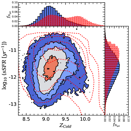
What are the properties of Gal-dens galaxies? We can divide Gal-dens into two distinct populations (A) and (B) using a sliding cut in SFR depending on sSFR . Population (A) galaxies are low-starforming ($\textsc{{SFR}}\sim 0.05$ ${\rm{M_{\odot}yr^{-1}}}$) and live in low-mass haloes (${{M_{\rm 200c}}}<10^{13.3}$ ${\rm{M_{\odot}}}$) while Population (B) are starforming ($0.1<\textsc{{SFR}}<0.3$ ${\rm{M_{\odot}yr^{-1}}}$) residing in most massive haloes (${{M_{\rm 200c}}}>10^{13.3}$ ${\rm{M_{\odot}}}$). We find a strong dependency on halo mass at fixed sSFR where low-mass haloes have a linear relation between SFR and sSFR, while the high-mass haloes exhibit larger SFRs at fixed sSFR. Furthermore, certain galaxy properties related to star formation can be clearly mapped onto Population (A) or (B) but other properties such as $M_{*}$ or (r-i)-colour are continuously distributed. This trend is particularly interesting because it shows the importance of secondary parameters related to the clustering besides halo mass as suggested by Wang et al. (2013).

How do gas-phase properties divide the sample into two distinct populations? In Fig. 10 we show the gas-phase metallicity $Z_{\rm Cold}$, a proxy for gas-cooling and star formation (Lebouteiller et al., 2013), for central galaxies. The two populations (A) and (B) are reflected in the bimodal distribution of $Z_{\rm Cold}$ where $\sim 80\%$ of Population (A) shows ${{Z_{\rm Cold}}}>9.5$ and only 20% lower values with ${{Z_{\rm Cold}}}\sim 9.5$. The opposite is true for Population (B). Common studies of fundamental relations between metallicity, mass, and star formation suggest that less/more massive galaxies have also lower/higher metal abundances (Lara-López et al., 2009; Yates et al., 2012). Our results show that Population (B)’s galaxies are more massive but have lower metal abundances. This “turnover” was also reported by Yates et al. (2012) for modelled galaxies at $z=0$ and is possibly linked to the infall of metal-poor gas after a gas-rich merger. In Yates & Kauffmann (2014) the same authors studied massive galaxies and divide them into an “enriching” and a “diluting” sample, the later show similar trends as our Population (B): low sSFR, lower $Z_{\rm Cold}$  and higher $M_{\rm BH}$. Furthermore, our findings are in total agreement with Lara-Lopez et al. (2013) showing that galaxies with low sSFR have high/low values of $Z_{\rm Cold}$ when $M_{\rm Cold}$ is low/high. We emphasise that the distinct separation of the two populations could give clues about galaxy evolution in the context of the origin of the fundamental luminosity/mass-metallicity relation, merger-induced star formation, or “downsizing” (Mannucci et al., 2010, see their Sec.1 for comparison).

How do the Populations (A) and (B) relate to environment? We expect that Population (A) fixes the clustering amplitude due to their environment as well as their number density. To this extent we apply the Vweb method (see Appendix A for details) to the underlying dark matter MDPL2 simulation. We show in the second column of Table 2 that more galaxies in the Gal-cols sample (61 %) are assigned into knots than in the Gal-dens sample (52 %). We detect a clear environmental dependency of this sample where Populations (A) is dominated by filament galaxies (62% with only 26 % in knots), while Population (B) has more galaxies in the knots (54%) than in the filaments (44%).

sample name &	environment	fraction	$\log_{\rm 10}$($M_{\rm 200c}$ [${\rm{M_{\odot}}}$])	$\log_{\rm 10}$($M_{*}$ [${\rm{M_{\odot}}}$])	$\log_{\rm 10}$(sSFR [$\rm yr^{-1}$])	$Z_{\rm Cold}$	$\log_{\rm 10}$(${{M_{\rm Cold}}}/{{M_{*}}}$)	$\log_{\rm 10}$($M_{\rm BH}$ [${\rm{M_{\odot}}}$])
population		of galaxies
Gal-cols	knot	0.61	13.79${}^{+0.21}_{-0.19}$	11.44${}^{+0.11}_{-0.09}$	-11.77${}^{+0.35}_{-0.37}$	9.10${}^{+0.18}_{-0.16}$	-1.14${}^{+0.20}_{-0.26}$	8.65${}^{+0.21}_{-0.19}$
Gal-cols	filament	0.37	13.57${}^{+0.19}_{-0.17}$	11.37${}^{+0.09}_{-0.05}$	-11.52${}^{+0.30}_{-0.34}$	9.18${}^{+0.21}_{-0.17}$	-1.25${}^{+0.22}_{-0.30}$	8.53${}^{+0.19}_{-0.16}$
Gal-dens	knot	0.52	13.55${}^{+0.27}_{-0.28}$	11.28${}^{+0.15}_{-0.14}$	-11.53${}^{+0.36}_{-0.42}$	9.25${}^{+0.36}_{-0.23}$	-1.35${}^{+0.31}_{-0.65}$	8.43${}^{+0.26}_{-0.26}$
Gal-dens	filament	0.41	13.22${}^{+0.23}_{-0.26}$	11.14${}^{+0.13}_{-0.14}$	-11.36${}^{+0.32}_{-0.44}$	9.55${}^{+0.30}_{-0.35}$	-1.83${}^{+0.54}_{-0.77}$	8.20${}^{+0.25}_{-0.24}$
Gal-dens  Pop (A)	knot	0.26	13.13${}^{+0.32}_{-0.34}$	11.05${}^{+0.07}_{-0.09}$	-11.40${}^{+0.38}_{-0.53}$	9.76${}^{+0.19}_{-0.29}$	-2.32${}^{+0.61}_{-0.71}$	8.05${}^{+0.19}_{-0.17}$
Gal-dens Pop (A)	filament	0.62	13.01${}^{+0.22}_{-0.22}$	11.02${}^{+0.08}_{-0.11}$	-11.40${}^{+0.39}_{-0.58}$	9.80${}^{+0.19}_{-0.25}$	-2.42${}^{+0.57}_{-0.74}$	8.00${}^{+0.17}_{-0.16}$
Gal-dens Pop (B)	knot	0.54	13.69${}^{+0.23}_{-0.21}$	11.36${}^{+0.13}_{-0.09}$	-11.58${}^{+0.35}_{-0.40}$	9.13${}^{+0.21}_{-0.17}$	-1.18${}^{+0.21}_{-0.31}$	8.56${}^{+0.22}_{-0.20}$
Gal-dens Pop (B)	filament	0.44	13.46${}^{+0.18}_{-0.16}$	11.29${}^{+0.09}_{-0.07}$	-11.33${}^{+0.26}_{-0.32}$	9.23${}^{+0.23}_{-0.19}$	-1.33${}^{+0.26}_{-0.34}$	8.42${}^{+0.20}_{-0.16}$
(i)	(ii)	(iii)	(iv)	(v)	(vi)	(vii)	(viii)	(ix)

Table 2: The table summarises the median and 1^st (sub-scripted) and 3^rd (super-scripted) quartile values of various galaxy properties for central galaxies in different environments and mock galaxy samples. Column (i) states the name of the CMASS-mock sample (and population if given). Thereby “Pop (A)” refers to Population (A) and “Pop (B)” to Population (B). Column (ii) indicates the environment (knot or filament) and (iii) their corresponding fraction. Results for the median values of halo mass $M_{\rm 200c}$, stellar mass $M_{*}$, specific star formation rate sSFR, gas-phase metallicity $Z_{\rm Cold}$, cold-gas fraction ${{M_{\rm Cold}}}/{{M_{*}}}$, and black hole mass $M_{\rm BH}$, respectively, are given in columns (iv)-(ix). Note that we only analysed galaxies in knots and filaments if their number of objects is significantly high, otherwise results for the whole sample is give as for Gal-cols.

Do galaxy properties have a dependency on environment? Besides the number fraction of galaxies, we further detail the sample properties in different environments in Table 2. Galaxies in filaments generally tend to have lower halo, stellar and black hole masses as well as sSFR and cold-gas fraction compared to the ones (from the same sample) in knots, while the cold-gas metallicity is normally higher in filaments than in knots. It is worth to note that Population (A) has significantly smaller halo mass, stellar mass, cold-gas fraction, and black hole mass than Population (B) in both environments, but significantly higher cold-gas metallicity in (A) than in (B).

What conclusion can we draw from the environmental dependency of galaxy properties? The star formation is not sufficiently suppressed in Population (B) and the most massive galaxies which should be “red-and-dead” are still starforming at a low rate. Therefore, Galacticus shows a higher abundance in the high-mass end of the SMF compared to the observed CMASS galaxy sample. Furthermore, most of the low-SFR galaxies in the Gal-dens sample live in the filaments in Population (A) with relatively lower $M_{\rm BH}$ and $M_{\rm Cold}$. They are located in haloes with suppressed star formation and could not grow in mass enough to exhibit brighter luminosities. This scenario is supported by the fact that Population (A) of Gal-dens has small contents of cold gas and as smaller cold-gas fractions in both knots and filaments, compared to Population (B). We cannot explicitly say why $M_{\rm Cold}$ is significantly smaller but it would imply that the quenching process in Galacticus is mostly dominated by tidal stripping of the cold gas instead of AGN feedback. We find it further interesting that half of the galaxies of this population exhibit higher gas-phase metallicities. We could speculate that the two populations (A) and (B) might have formed at different times and evolved differently due to their environment (see “environmental quenching” of star formation e.g. Tomczak et al. 2018) or halo masses (see “halo quenching” of low-mass central galaxies e.g. Tal et al. 2014). Different evolutionary paths (as Montero-Dorta et al. 2017b have shown for BOSS) might have contributed to the variations in the intrinsic scatter and could also provide a signal of the assembly bias, however, further studies are required to provide proof of that hypothesis.

How is the environmental dependency reflected in the clustering? We expect that the different quenching processes have a crucial impact on the intrinsic scatter in stellar mass at fixed halo mass, ${{\sigma_{\log_{\rm 10}{{M_{*}}}}}}$, which in return has an impact on the clustering amplitude. Compared to other works we report that the values of the intrinsic scatter of Gal-cols and Gal-mass with 0.1 dex and Gal-dens with 0.15 dex depending on the halo mass. Those results are similar to Rodríguez-Torres et al. (2016), who found a scatter of 0.14 dex for their CMASS abundance matching BigMD-LC. However, Shankar et al. (2014) stated that an intrinsic scatter of at least 0.15 dex is needed to reproduce the BOSS clustering which means that Galacticus in general shows an insufficient level of scatter. Furthermore, Tinker et al. (2017) reported a slightly larger observed scatter of ${{{{\sigma_{\rm{log}{{M_{*}}}}}}}}=0.18^{+0.01}_{-0.02}$ dex for CMASS and Leauthaud et al. (2012) of $0.249\pm 0.019$ dex measured from passive galaxies in the COSMOS survey (Scoville et al., 2007). Gu et al. (2016) found similar values for the intrinsic scatter ${{{{\sigma_{\rm{log}{{M_{*}}}}}}}}<0.2$ and emphasise that the origin of the scatter in the SHMF at higher masses is induced by the hierarchical assembly, while at low halo masses it is associated with in-situ growth. Smaller scatter could mean that there is insufficient scatter in the assembly histories, or that the galaxy formation models do not capture all of it. However, understanding this issue is a non-trivial task and one has to address model specific properties in more detail to understand which combination of properties causes this effect. We find that the comparison with other SAMs would help on this task, but would be beyond the scope of this paper and is therefore left for further studies.

7 Summary

Our work is based on the Baryon Oscillation Spectroscopic Survey (BOSS, Schlegel et al., 2009; Dawson et al., 2013) of the Sloan Digital Sky Survey (SDSS-III, Eisenstein et al., 2011) CMASS (for “constant mass”) sample and a semi-analytical model of galaxy formation (SAM), called Galacticus, as part of the MultiDark-Galaxies products (Knebe et al., 2018). The CMASS sample was build from the SDSS-III/BOSS survey catalogues by applying a complex colour-magnitude selection (see Eq. (1)-(4)). We use the same selection scheme to extract our modelled galaxy catalogue from Galacticus, called Gal-cols, at $z=0.56$.

We provide detail assessment of the SAM via comparing with BOSS as well as results on the galaxy-halo connection and clustering studies of the 2-point correlation function. For reasons stated in Section 3, we construct two additional CMASS-mock samples. The first one is called Gal-dens and was build by randomly selecting modelled galaxies (or down-sampling) until they fit the observational SMF of BOSS between $0.5<z<0.6$. The second CMASS-mock is called Gal-mass and was generated by applying a high stellar mass cut of ${{M_{*}}}>10^{11.24}$ ${\rm{M_{\odot}}}$ as introduced by Maraston et al. (2013). Here we summarise our major results of our study:

1. The Galacticus colour-magnitude selected CMASS-mock sample, Gal-cols, shows a lower number density, fewer blue objects, and is located within a smaller parameter space compared to the observational sample (see Fig. 1). Its red sequence is intrinsically concentrated, as predicted by Montero-Dorta et al. (2016) (see Fig. 2). Although the number density of this sample is only 1/3 the density of BOSS galaxies, Gal-cols overpredicts red galaxies at ${{M_{*}}}\mathrel{\hbox{\hbox to0.0pt{\hbox{\lower 4.0pt\hbox{$\sim$}}\hss}\hbox{$>$}}}10^{12}$ ${\rm{M_{\odot}}}$ (see Fig. 4). Galaxies in Gal-dens satisfy the CMASS colour selection criteria, but they did not enter the sample selection due to their luminosities being approx. 1.5-2 magnitudes lower in $i$-band (see middle panel of Fig. 3).

2. Galacticus Gal-cols and Gal-mass samples agree very well with the stellar to halo mass relation of Rodríguez-Torres et al. (2016) and weak-lensing results from Shan et al. (2017), while Gal-dens shows similar behaviour as the halo abundance matching model from Behroozi et al. (2013) (see Fig. 6). However, all three CMASS-mock samples exhibit an increasing scatter at fixed halo mass from ${{{{\sigma_{\rm{log}{{M_{*}}}}}}}}\sim 0.05-0.15$ dex depending on halo mass. Compared to other works with ${{{{\sigma_{\rm{log}{{M_{*}}}}}}}}=0.14$ dex by Rodríguez-Torres et al. (2016), ${{{{\sigma_{\rm{log}{{M_{*}}}}}}}}=0.18^{+0.01}_{-0.02}$ dex by Tinker et al. (2017) or $0.249\pm 0.019$ dex by Leauthaud et al. (2012), Galacticus displays an insufficient level of scatter.

3. Gal-cols and Gal-mass agree poorly with the clustering of CMASS galaxies from the high-fidelity mock BigMD-LC (Rodríguez-Torres et al., 2016), which was obtained using halo abundance matching techniques. We find that the combination of low intrinsic scatter at fixed halo mass and missing objects (or objects being too faint) is responsible for the high clustering amplitudes of Gal-cols and Gal-mass. However, the Gal-dens sample reproduces the clustering of central and satellite galaxies as well as of centrals only, within 1$\sigma$ (see Fig. 8).

4. We can divide the Gal-cols and Gal-dens samples into two sub-populations, (A) and (B), using a given SFR cut. Population  (A) corresponds to low-starforming galaxies in lower-mass haloes, while Population (B) is comprised by mildly-starforming galaxies living in the most massive haloes. (A)-galaxies were found as the population which displays too faint luminosities as mentioned in (i), but fix the clustering amplitude due to the environmental affiniation and number density. By using the Vweb code (see Appendix A) we confirm that (A)-galaxies live in filaments, while (B)-galaxies can be found in knots.

5. We find further correlations between halo mass $M_{\rm 200c}$ and star formation related properties as (specific) star formation rate, gas-phase metallicity, $Z_{\rm cold}$, and cold-gas fraction, ${{M_{\rm Cold}}}/{{M_{*}}}$, but also black hole mass $M_{\rm BH}$, depending on the environment and sub-population (A) and (B) where e.g. 80% of galaxies in Population (A) show higher sSFR and $Z_{\rm cold}>9.5$, but lower cold-gas fractions and black hole masses compared to their counterparts in Population (B) (see Table 2).

In this work, we have carefully examined several samples of the most massive galaxies from the Galacticus galaxy formation model. In a follow-up work, we plan to extend this analysis to other semi-analytical models in order to study in more detail the star formation history of massive galaxies at intermediate redshifts. This follow-up study will be connected to the effect of galaxy assembly bias, a crucial aspect to the formation and evolution of galaxies.

Appendix A The Vweb method

This Vweb method applies the shear tensor technique classify the large-scale environments into either “void”, “sheet”, “filament”, or “knot”. Following Hoffman et al. (2012), the velocity shear tensor is defined as

$$\Sigma_{\alpha\beta}=-\frac{1}{2H_{0}}\left(\frac{\partial v_{\alpha}}{\partial r_{\beta}}+\frac{\partial v_{\beta}}{\partial r_{\alpha}}\right),$$ (14)

where, $H_{0}$ is the Hubble constant. The eigenvalues of $\Sigma_{\alpha\beta}$ are denoted as $\lambda_{i}$ ($i$ = 1, 2 and 3).

The simulation box is separated into cubic mesh cells, within which the velocity field is calculated. Each cell has a size of $\sim 1$ Mpc. After smoothing the velocity field, we calculate the eigenvalues of the velocity shear tensor in each cell. Each cell is then classified as either ‘void’, ‘sheet’, ‘filament’, or ‘knot’ according to the eigenvalues $\lambda_{1}>\lambda_{2}>\lambda_{3}$:

• void, if $\lambda_{1}<\lambda_{th}$,

• sheet, if $\lambda_{1}\geq\lambda_{th}>\lambda_{2}$,

• filament, if $\lambda_{2}\geq\lambda_{th}>\lambda_{3}$,

• knot, if $\lambda_{3}\geq\lambda_{th}$,

where $\lambda_{th}$ is a free threshold parameter (Hoffman et al., 2012; Libeskind et al., 2012, 2013). Following the discussion of Carlesi et al. (2014); Cui et al. (2018, 2019), we set $\lambda_{th}=0.1$, which presents better agreement to the visualised density field. Our mock galaxies are then placed onto the same grid checking for the web classification of the cell they lie in.

References

- Alam et al. (2015) Alam S., et al., 2015, ApJS, 219, 12
- Alam et al. (2017) Alam S., Ata M., Bailey S. e. a., 2017, MNRAS, 470, 2617
- Allende Prieto et al. (2001) Allende Prieto C., Lambert D. L., Asplund M., 2001, ApJ, 556, L63
- Almeida et al. (2008) Almeida C., Baugh C. M., Wake D. A., Lacey C. G., Benson A. J., Bower R. G., Pimbblet K., 2008, MNRAS, 386, 2145
- Anderson et al. (2014) Anderson L., Aubourg É., Bailey S., et al. 2014, MNRAS, 441, 24
- Asplund et al. (2009) Asplund M., Grevesse N., Sauval A. J., Scott P., 2009, ARA&A, 47, 481
- Baugh (2006) Baugh C. M., 2006, Rep. Prog. Phys., 69, 3101
- Baugh (2013) Baugh C. M., 2013, in The Intriguing Life of Massive Galaxies. pp 191–199, doi:10.1017/S1743921313004778
- Behroozi et al. (2013) Behroozi P. S., Wechsler R. H., Conroy C., 2013, ApJ, 770, 57
- Behroozi et al. (2013a) Behroozi P. S., Wechsler R. H., Wu H.-Y., 2013a, ApJ, 762, 109
- Behroozi et al. (2013b) Behroozi P. S., Wechsler R. H., Wu H.-Y., Busha M. T., Klypin A. A., Primack J. R., 2013b, ApJ, 763, 18
- Benson (2010) Benson A. J., 2010, Phys. Rep., 495, 33
- Benson (2012) Benson A. J., 2012, New Astron., 17, 175
- Benson et al. (2000) Benson A. J., Cole S., Frenk C. S., Baugh C. M., Lacey C. G., 2000, MNRAS, 311, 793
- Benson et al. (2003) Benson A. J., Bower R. G., Frenk C. S., Lacey C. G., Baugh C. M., Cole S., 2003, ApJ, 599, 38
- Berlind et al. (2003) Berlind A. A., et al., 2003, ApJ, 593, 1
- Bernardi et al. (2016) Bernardi M., Meert A., Sheth R. K., Huertas-Company M., Maraston C., Shankar F., Vikram V., 2016, MNRAS, 455, 4122
- Beutler et al. (2014) Beutler F., et al., 2014, MNRAS, 444, 3501
- Blanton & Roweis (2007) Blanton M. R., Roweis S., 2007, AJ, 133, 734
- Bower et al. (2006) Bower R. G., Benson A. J., Malbon R., Helly J. C., Frenk C. S., Baugh C. M., Cole S., Lacey C. G., 2006, MNRAS, 370, 645
- Bryan & Norman (1998) Bryan G. L., Norman M. L., 1998, ApJ, 495, 80
- Campbell et al. (2015) Campbell D. J. R., et al., 2015, MNRAS, 452, 852
- Cannon et al. (2006) Cannon R., Drinkwater M., Edge A., et al. 2006, MNRAS, 372, 425
- Carlesi et al. (2014) Carlesi E., Knebe A., Lewis G. F., Wales S., Yepes G., 2014, MNRAS, 439, 2943
- Chabrier (2003) Chabrier G., 2003, PASP, 115, 763
- Chuang et al. (2016) Chuang C.-H., Prada F., Pellejero-Ibanez M., et al. 2016, MNRAS, 461, 3781
- Collacchioni et al. (2018) Collacchioni F., Cora S. A., Lagos C. D. P., Vega-Martínez C. A., 2018, MNRAS, 481, 954
- Conroy et al. (2009) Conroy C., Gunn J. E., White M., 2009, ApJ, 699, 486
- Contreras et al. (2013) Contreras C., et al., 2013, MNRAS, 430, 924
- Contreras et al. (2015) Contreras S., Baugh C. M., Norberg P., Padilla N., 2015, MNRAS, 452, 1861
- Cora (2016) Cora S. A., 2016, Boletin de la Asociacion Argentina de Astronomia La Plata Argentina, 58, 8
- Cora et al. (2018) Cora S. A., Hough T., Vega-Martínez C. A., Orsi Á. A., 2018, MNRAS, p. 3059
- Cuesta et al. (2016) Cuesta A. J., Vargas-Magaña M., Beutler F., et al. 2016, MNRAS, 457, 1770
- Cui et al. (2018) Cui W., Knebe A., Yepes G., Yang X., Borgani S., Kang X., Power C., Staveley-Smith L., 2018, MNRAS, 473, 68
- Cui et al. (2019) Cui W., et al., 2019, MNRAS submitted
- Dawson et al. (2013) Dawson K. S., Schlegel D. J., Ahn C. P., Anderson S. F., Aubourg É., Bailey S., et al. 2013, AJ, 145, 10
- Eisenstein et al. (2001) Eisenstein D. J., Annis J., Gunn J. E., et al. 2001, AJ, 122, 2267
- Eisenstein et al. (2011) Eisenstein D. J., et al., 2011, AJ, 142, 72
- Farrow et al. (2015) Farrow D. J., et al., 2015, MNRAS, 454, 2120
- Favole et al. (2016) Favole G., McBride C. K., Eisenstein D. J., Prada F., Swanson M. E., Chuang C.-H., Schneider D. P., 2016, MNRAS, 462, 2218
- Ferrara et al. (1999) Ferrara A., Bianchi S., Cimatti A., Giovanardi C., 1999, ApJS, 123, 437
- Fukugita et al. (1996) Fukugita M., Ichikawa T., Gunn J. E., Doi M., Shimasaku K., Schneider D. P., 1996, AJ, 111, 1748
- Gil-Marín et al. (2017) Gil-Marín H., Percival W. J., Verde L., Brownstein J. R., Chuang C.-H., Kitaura F.-S., Rodríguez-Torres S. A., Olmstead M. D., 2017, MNRAS, 465, 1757
- Gonzalez-Perez et al. (2014) Gonzalez-Perez V., Lacey C. G., Baugh C. M., Lagos C. D. P., Helly J., Campbell D. J. R., Mitchell P. D., 2014, MNRAS, 439, 264
- Gruppioni et al. (2015) Gruppioni C., et al., 2015, MNRAS, 451, 3419
- Gu et al. (2016) Gu M., Conroy C., Behroozi P., 2016, ApJ, 833, 2
- Guo et al. (2013) Guo H., Zehavi I., Zheng Z., et al. 2013, ApJ, 767, 122
- Guo et al. (2014) Guo H., et al., 2014, MNRAS, 441, 2398
- Guo et al. (2018) Guo H., Yang X., Lu Y., 2018, ApJ, 858, 30
- Henriques et al. (2017) Henriques B. M. B., White S. D. M., Thomas P. A., Angulo R. E., Guo Q., Lemson G., Wang W., 2017, MNRAS, 469, 2626
- Henriques et al. (2018) Henriques B., White S., Lilly S., Bell E., Bluck A., Terrazas B., 2018, arXiv e-prints, p. arXiv:1809.01154
- Hoffman et al. (2012) Hoffman Y., Metuki O., Yepes G., Gottlöber S., Forero-Romero J. E., Libeskind N. I., Knebe A., 2012, MNRAS, 425, 2049
- Hunter (2007) Hunter J. D., 2007, Computing in Science and Engineering, 9, 90
- Kitaura et al. (2016) Kitaura F.-S., Rodríguez-Torres S., Chuang C.-H., et al. 2016, MNRAS, 456, 4156
- Klypin et al. (2016) Klypin A., Yepes G., Gottlöber S., Prada F., Heß S., 2016, MNRAS, 457, 4340
- Knebe et al. (2018) Knebe A., Stoppacher D., Prada F., et al. 2018, MNRAS, 474, 5206
- Kroupa (2001) Kroupa P., 2001, MNRAS, 322, 231
- Lacey et al. (2016) Lacey C. G., et al., 2016, MNRAS, 462, 3854
- Lagos et al. (2014) Lagos C. D. P., Baugh C. M., Zwaan M. A., Lacey C. G., Gonzalez-Perez V., Power C., Swinbank A. M., van Kampen E., 2014, MNRAS, 440, 920
- Landy & Szalay (1993) Landy S. D., Szalay A. S., 1993, ApJ, 412, 64
- Lara-López et al. (2009) Lara-López M. A., Cepa J., Bongiovanni A., Pérez García A. M., Castañeda H., Fernández Lorenzo M., Pović M., Sánchez-Portal M., 2009, A&A, 505, 529
- Lara-Lopez et al. (2013) Lara-Lopez M. A., et al., 2013, MNRAS, 433, L35
- Leauthaud et al. (2011) Leauthaud A., Tinker J., Behroozi P. S., Busha M. T., Wechsler R. H., 2011, ApJ, 738, 45
- Leauthaud et al. (2012) Leauthaud A., Tinker J., Bundy K., et al. 2012, ApJ, 744, 159
- Lebouteiller et al. (2013) Lebouteiller V., Heap S., Hubeny I., Kunth D., 2013, A&A, 553, A16
- Libeskind et al. (2012) Libeskind N. I., Hoffman Y., Knebe A., Steinmetz M., Gottlöber S., Metuki O., Yepes G., 2012, MNRAS, 421, L137
- Libeskind et al. (2013) Libeskind N. I., Hoffman Y., Forero-Romero J., Gottlöber S., Knebe A., Steinmetz M., Klypin A., 2013, MNRAS, 428, 2489
- Lietzen et al. (2012) Lietzen H., Tempel E., Heinämäki P., Nurmi P., Einasto M., Saar E., 2012, A&A, 545, A104
- Liu et al. (2016) Liu G. C., Lu Y. J., Xie L. Z., Chen X. L., Zhao Y. H., 2016, A&A, 585, A52
- Łokas & Mamon (2001) Łokas E. L., Mamon G. A., 2001, MNRAS, 321, 155
- Mannucci et al. (2010) Mannucci F., Cresci G., Maiolino R., Marconi A., Gnerucci A., 2010, MNRAS, 408, 2115
- Maraston (2005) Maraston C., 2005, MNRAS, 362, 799
- Maraston et al. (2006) Maraston C., Daddi E., Renzini A., Cimatti A., Dickinson M., Papovich C., Pasquali A., Pirzkal N., 2006, ApJ, 652, 85
- Maraston et al. (2009) Maraston C., Strömbäck G., Thomas D., Wake D. A., Nichol R. C., 2009, MNRAS, 394, L107
- Maraston et al. (2013) Maraston C., et al., 2013, MNRAS, 435, 2764
- Masters et al. (2011) Masters K. L., Maraston C., Nichol R. C., et al. 2011, MNRAS, 418, 1055
- Montero-Dorta et al. (2016) Montero-Dorta A. D., et al., 2016, MNRAS, 461, 1131
- Montero-Dorta et al. (2017a) Montero-Dorta A. D., Bolton A. S., Shu Y., 2017a, MNRAS, 468, 47
- Montero-Dorta et al. (2017b) Montero-Dorta A. D., et al., 2017b, ApJ, 848, L2
- More et al. (2011) More S., van den Bosch F. C., Cacciato M., Skibba R., Mo H. J., Yang X., 2011, MNRAS, 410, 210
- Moster et al. (2010) Moster B. P., Somerville R. S., Maulbetsch C., van den Bosch F. C., Macciò A. V., Naab T., Oser L., 2010, ApJ, 710, 903
- Moustakas et al. (2013) Moustakas J., et al., 2013, ApJ, 767, 50
- Mueller et al. (2018) Mueller E.-M., Percival W., Linder E., Alam S., Zhao G.-B., Sánchez A. G., Beutler F., Brinkmann J., 2018, MNRAS, 475, 2122
- Mutch et al. (2013) Mutch S. J., Poole G. B., Croton D. J., 2013, MNRAS, 428, 2001
- Navarro et al. (1997) Navarro J. F., Frenk C. S., White S. D. M., 1997, ApJ, 490, 493
- Nuza et al. (2013) Nuza S. E., Sánchez A. G., Prada F., et al. 2013, MNRAS, 432, 743
- Orsi et al. (2014) Orsi Á., Padilla N., Groves B., Cora S., Tecce T., Gargiulo I., Ruiz A., 2014, MNRAS, 443, 799
- Planck Collaboration et al. (2015) Planck Collaboration et al., 2015, preprint, (arXiv:1502.01589)
- Reid et al. (2014) Reid B. A., Seo H.-J., Leauthaud A., Tinker J. L., White M., 2014, MNRAS, 444, 476
- Reid et al. (2016) Reid B., Ho S., Padmanabhan N., et al. 2016, MNRAS, 455, 1553
- Ren et al. (2018) Ren K., Trenti M., Mutch S. J., 2018, ApJ, 856, 81
- Rodrigues et al. (2017) Rodrigues L. F. S., Vernon I., Bower R. G., 2017, MNRAS, 466, 2418
- Rodríguez-Torres et al. (2016) Rodríguez-Torres S. A., et al., 2016, MNRAS, 460, 1173
- Ross et al. (2017) Ross A. J., et al., 2017, MNRAS, 472, 4456
- Saito et al. (2016) Saito S., et al., 2016, MNRAS, 460, 1457
- Schlegel et al. (2009) Schlegel D., White M., Eisenstein D., 2009, in astro2010: The Astronomy and Astrophysics Decadal Survey. (arXiv:0902.4680)
- Scoville et al. (2007) Scoville N., Aussel H., Brusa M., et al. 2007, The Astrophysical Journal Supplement Series, 172, 1
- Shan et al. (2017) Shan H., et al., 2017, ApJ, 840, 104
- Shankar et al. (2014) Shankar F., et al., 2014, MNRAS, 439, 3189
- Shirakata et al. (2018) Shirakata H., et al., 2018, preprint, p. arXiv:1802.02169 (arXiv:1802.02169)
- Sinha (2016) Sinha M., 2016, Corrfunc: Corrfunc-1.1.0, doi:10.5281/zenodo.55161, http://dx.doi.org/10.5281/zenodo.55161
- Somerville & Davé (2015) Somerville R. S., Davé R., 2015, ARA&A, 53, 51
- Springel et al. (2005) Springel V., et al., 2005, Nature, 435, 629
- Sullivan et al. (2017) Sullivan J. M., Wiegand A., Eisenstein D. J., 2017, preprint, p. arXiv:1711.09899 (arXiv:1711.09899)
- Tal et al. (2014) Tal T., et al., 2014, ApJ, 789, 164
- Tinker et al. (2013) Tinker J. L., Leauthaud A., Bundy K., George M. R., Behroozi P., Massey R., Rhodes J., Wechsler R. H., 2013, ApJ, 778, 93
- Tinker et al. (2017) Tinker J. L., et al., 2017, ApJ, 839, 121
- Tomczak et al. (2018) Tomczak A. R., et al., 2018, arXiv e-prints, p. arXiv:1812.04633
- Wang et al. (2013) Wang L., De Lucia G., Weinmann S. M., 2013, MNRAS, 431, 600
- Wechsler & Tinker (2018) Wechsler R. H., Tinker J. L., 2018, preprint, p. arXiv:1804.03097 (arXiv:1804.03097)
- White & Frenk (1991) White S. D. M., Frenk C. S., 1991, ApJ, 379, 52
- White et al. (2011) White M., Blanton M., Bolton A., et al. 2011, ApJ, 728, 126
- Xie et al. (2017) Xie L., De Lucia G., Hirschmann M., Fontanot F., Zoldan A., 2017, MNRAS, 469, 968
- Yates & Kauffmann (2014) Yates R. M., Kauffmann G., 2014, MNRAS, 439, 3817
- Yates et al. (2012) Yates R. M., Kauffmann G., Guo Q., 2012, MNRAS, 422, 215
- Zheng et al. (2005) Zheng Z., et al., 2005, ApJ, 633, 791
- Zoldan et al. (2018) Zoldan A., De Lucia G., Xie L., Fontanot F., Hirschmann M., 2018, preprint, p. arXiv:1803.08056 (arXiv:1803.08056)
- van Daalen et al. (2016) van Daalen M. P., Henriques B. M. B., Angulo R. E., White S. D. M., 2016, MNRAS, 458, 934