A comprehensive statistical study on gamma-ray bursts

Abstract

In order to obtain an overview of the gamma-ray bursts (GRBs), we need a full sample. In this paper, we collected 6289 GRBs (from GRB 910421 to GRB 160509A) from the literature, including prompt emission, afterglow and host galaxy properties. We hope to use this large sample to reveal the intrinsic properties of GRB. We have listed all the data in machine readable tables, including the properties of the GRBs, correlation coefficients and linear regression results of two arbitrary parameters, and linear regression results of any three parameters. These machine readable tables could be used as a data reservoir for further studies on the classifications or correlations. One may find some intrinsic properties from these statistical results. With this comprehensive table, it is possible to find relations between different parameters, and to classify the GRBs into different kinds of sub-groups. With the completion, it may reveal the nature of GRBs and may be used as tools like pseudo-redshift indicators, standard candles, etc. All the machine readable data and statistical results are available on the website of the journal.

1 Introduction

Gamma-ray bursts (GRBs) were firstly detected in 1967 (Klebesadel et al., 1973) by the Vela Satellite Network. They have been intensely studied since 1990s, especially after the operation of Burst and Transient Source Experiment (BATSE) onboard Compton Gamma Ray Observatory (CGRO) (Meegan et al., 1992). For a single event, the fluence is between $10^{\rm-7}$ and $10^{\rm-5}$ $\rm ergs~{}cm^{\rm-2}$, and the isotropic energy is from about $10^{\rm 48}$ to $10^{\rm 55}$ $\rm ergs$ (Nakar, 2007; Zhang et al., 2011; Gehrels & Razzaque, 2013; Berger, 2014; Kumar & Zhang, 2015). So GRBs are the most violent and energetic stellar explosions known to humankind in distant galaxies (Kumar & Zhang, 2015). The nature of GRBs is still under discovered even though there are many researches have been going on for many years. Fireball model is one of historical models to explain the mechanism of GRBs (Rees & Meszaros, 1992; Piran et al., 1993; Wijers et al., 1997; Mészáros, 1998, 2006), which implies GRBs are produced by highly relativistic and collimated jets. Interaction of blobs in the jet is believed to produce the prompt emission, and the interaction of the jet with the ambient material produces the multi-wavelength afterglow (X-ray, optical and sometimes also radio). For a clear understanding of the current situation for GRBs, some recent reviews could be read, such as Piran (1999, 2004); Zhang & Mészáros (2004); Mészáros (2006); Zhang (2007); Kumar & Zhang (2015) for the general physics, Nakar (2007); Berger (2014) for short GRBs, Gehrels et al. (2009) concentrating on the observations, Woosley & Bloom (2006); Maeder & Meynet (2012) on the progenitors, and Lee et al. (2000) on the central engines.

In order to explain the physics of GRBs, many attempts have been made to describe the spectra in different physical frameworks, and significant progress is achieved. There are two main frameworks. One is internal or external shocks, the emissions are assumed to be non-thermal intrinsically (Katz, 1994; Rees & Meszaros, 1994; Tavani, 1996; Sari et al., 1998; Gao et al., 2015b). Another is photospheric emission, which is predicted to occur in the “fireball” model (Mészáros & Rees, 2000; Rees & Mészáros, 2005; Pe’er et al., 2007; Thompson et al., 2007). Racz et al. (2017) found the synchrotron radiation is significant in Fermi/Gamma-ray Burst Monitor (GBM) spectra. Sub-photospheric dissipation (Rees & Mészáros, 2005; Pe’er et al., 2006a; Giannios, 2006; Chhotray & Lazzati, 2015) was suggested as the emission mechanism in some bursts which can broaden the spectrum. Ahlgren et al. (2015) firstly provided a full physical model, DREAM (Dissipation with Radiative Emission as A table Model), which is based on sub-photospheric dissipation, and gave acceptable fits to GRB 090618 and GRB 100724B for more details. If we take sub-photospheric dissipation and/or high latitude effects (Lundman et al., 2013), the photospheric model can account for a large diversity of spectra. Recently, the spectra observations of GRBs show a mixture of thermal and non-thermal spectra (Ryde, 2005; Ryde & Pe’er, 2009; Guiriec et al., 2010; Nappo et al., 2017), which implies that there is an interplay between different emission mechanisms. The exist of GRBs subgroups might be the consequence of different emission mechanisms (Bégué & Burgess, 2016). Acuner & Ryde (2017) searched the full Fermi/GBM catalogue using Gaussian Mixture Models to cluster bursts according to their low energy photon index of Band model (Band et al., 1993) ($\alpha_{\rm band}$), high energy photon index of Band model ($\beta_{\rm band}$), spectral peak energy of Band model ($E_{\rm p,band}$), fluence ($F_{\rm g}$) and duration of 5% to 95% $\gamma$-ray fluence ($T_{\rm 90}$), in order to divide bursts into photospheric origin and synchrotron origin. They thought both emission from the photosphere and optically-thin synchrotron radiation are operating but different emissions dominate differently for individual GRBs. They found 1/3 of the bursts are consistent with synchrotron radiation, and 2/3 of all bursts are consistent with photospheric emission. Beside the two main groups, they also found subgroups. It is maybe due to the dissipation pattern in the jet, alternatively due to whether the jet is dominated by thermal or magnetic energy, or due to the viewing angle (Acuner & Ryde, 2017). For the afterglows of GRBs, we can also find thermal and non-thermal components. Up to now, there are totally 16 GRBs reported to have thermal components in the X-ray light curves (LCs) (Campana et al., 2006; Page et al., 2011; Thöne et al., 2011; Starling et al., 2011; Sparre & Starling, 2012; Starling et al., 2012; Friis & Watson, 2013; Nappo et al., 2017). Valan et al. (2017) reported six detections of additional thermal components in the GRBs’ early X-ray afterglows. A cocoon breaking out from a thick wind or late prompt emission maybe the explanation for the additional thermal components, which may be hidden by bright afterglows in the majority of GRBs. That is why small part of the afterglows detected with additional thermal components (Valan et al., 2017). Some other possible explanations are that shock break-out is appealing for GRBs with associated supernova (Campana et al., 2006), or the cocoon that surrounds the jet (Mészáros & Rees, 2001; Pe’er et al., 2006b; Ghisellini et al., 2007; Starling et al., 2012), or the jet itself (Friis & Watson, 2013; Irwin & Chevalier, 2016; Nappo et al., 2017).

With accumulated data, statistical study may reveal the underlying physics. It can be roughly split into classification and correlation seeking. Nowadays, the classification of GRBs is still in suspense. Traditionally, they are grouped into short GRBs (SGRBs) and long GRBs (LGRBs) depending on $T_{\rm 90}$ smaller or greater than 2 s, where $T_{\rm 90}$ is the time difference between the 95th and 5th percentile of the total counts, which is often taken as the typical duration of a GRB. Kouveliotou et al. (1993) analysed the $\log T_{\rm 90}$ distribution of 222 BATSE GRBs. They found that the distribution is a bimodal form, and the dividing line is about 2 $\rm s$. However, $T_{\rm 90}$ is a function of energy band. Consequently, this value is detector dependent (Bromberg et al., 2013; Resmi, 2017). Bromberg et al. (2013) calculated a useful threshold duration that separates collapsars (long) from non-collapsars (short), $T_{\rm 90}=3.1\pm 0.5$ s in BATSE, $T_{\rm 90}=1.7_{-0.6}^{+0.4}$ s in Fermi GBM, $T_{\rm 90}=0.8\pm 0.3$ s in Swift. LGRBs are rich in low-energy photons. They are thought to be originated from the gravitational collapse of massive stars, owing to the observational evidences of some LGRBs associated with Type Ic supernovae (SNe) (Galama et al., 1998; Hjorth et al., 2003; Stanek et al., 2003; Woosley & Bloom, 2006; Hjorth & Bloom, 2012; Xu et al., 2013). The host galaxies of LGRBs have low metallicity, sometimes interacting with other galaxies (Sahu et al., 1997; Bloom et al., 1998, 2002; Chary et al., 2002; Christensen et al., 2004; Savaglio et al., 2009; Krühler et al., 2015), high star-forming rate and small host galaxy offset (Bloom et al., 2002; Fruchter et al., 2006; Blanchard et al., 2016). Comparing to LGRBs, the SGRBs are rich in higher energetic photons. They are thought to be the product of compact binary mergers with at least one neutron star, such as a black hole and a neutron star (BH-NS), or two neutron stars (NS-NS) (Eichler et al., 1989; Paczynski, 1991; Narayan et al., 1992; Nakar, 2007; Zhang et al., 2009a). Although some studies preferred other compact merger models, like an ONeMg with a CO white dwarf (WD) merger model (Lyutikov & Toonen, 2017). The presence of kilonova emission (Berger et al., 2013; Tanvir et al., 2013) and the locations of SGRBs (Berger et al., 2013) provide evidences to compact merger model. Therefore SGRBs maybe the candidate sources of gravitational waves (GWs) (e.g., Eichler et al. (1989); Nakar (2007); Piro & Thrane (2012); Berger (2014)). Until now, advanced LIGO (Laser Interferometer Gravitational Wave Observatory) have detected some GWs, such as GW 150914 (Abbott et al., 2016a), GW151226 (Abbott et al., 2016b), GW170104 (Abbott et al., 2017a) and GW170817 (Abbott et al., 2017b). The observation of the association of GW170817 and GRB 170817A confirms the NS-NS as a progenitor of SGRBs (Abbott et al., 2017b; Xiao et al., 2017; Pozanenko et al., 2017; Goldstein et al., 2017; Abbott et al., 2017c; Zou et al., 2018; Granot et al., 2017). The host galaxies of SGRBs include late-type and early-type galaxies, and have large offset which is about 5 times larger than LGRBs (Fong et al., 2010a). Some SGRBs are putatively associated with r-process-powered “kilonovae/macronovae”, like GRB 130603B, GRB 060614, and probably GRB 080503, GRB 050709 as well (Li & Paczyński, 1998; Metzger et al., 2010; Tanvir et al., 2013; Berger et al., 2013; Yang et al., 2015; Gao et al., 2015a; Jin et al., 2016).

With an increasing number of instruments applied for detecting GRBs, such as $Beppo$SAX/GRBM (40 - 700 $\rm keV$) (Boella et al., 1997), Konus-Wind (10 keV - 10 MeV) (Aptekar et al., 1995), HETE-2 (6 - 400 $\rm keV$) (Ricker et al., 2003), INTEGRAL (15 - 200 $\rm keV$) (Mereghetti et al., 2003), Swift/XRT (0.2 - 10 $\rm keV$) (Gehrels et al., 2004; Burrows et al., 2005), Swift/BAT (15 - 150 $\rm keV$) (Gehrels et al., 2004; Barthelmy et al., 2005), Polar (10 - 500 $\rm keV$) (Produit et al., 2018), HXMT (10 - 500 $\rm keV$) (Zhang et al., 2014b), Fermi/LAT (20 MeV - 300 $\rm GeV$) (GLAST Facility Science Team et al., 1999; Ackermann et al., 2012), Fermi/GBM (8 keV - 40 $\rm MeV$) (GLAST Facility Science Team et al., 1999; Meegan et al., 2009), the Alpha Magnetic Spectrometer (AMS-02) (0.5 GeV - 2 TeV) (Kounine, 2012), the DArk Matter Particle Explorer (DAMPE, or called Wukong) (5 GeV -10 TeV) (Chang et al., 2017), we can have much better quality data for analyzing. Some researches argued that there maybe exits a third class of GRBs (e.g. de Ugarte Postigo et al., 2011). Tsutsui et al. (2013a) identified subclasses of LGRBs with cumulative light curve of the prompt emission. Different subclasses have different Fundamental Planes, which is a correlation between $L_{\rm pk}$, $E_{\rm pk}$ and $T_{\rm L}$ ($T_{\rm L}=E_{\rm iso}/L_{\rm pk}$) (Tsutsui et al., 2011). Forthermore, Tsutsui & Shigeyama (2014) confirmed that there do exist the third class in GRBs in addition to SGRBs and LGRBs. The classification method is based on two properties both quantified with light curve shapes of the prompt emission: the absolute deviation from the constant luminosity of their cumulative light curve, and the ratio of the mean counts to the maximum counts (Tsutsui et al., 2013a; Tsutsui & Shigeyama, 2014). A new class of GRBs with thousands of seconds of duration known as ultra-long bursts have been discovered (Stratta et al., 2013; Levan et al., 2014; Cucchiara et al., 2015; Horesh et al., 2015; Gompertz & Fruchter, 2017). The possible candidates for ultra-long bursts origin are blue supergiant collapsars, magnetars, and white dwarf tidal disruption events caused by massive black holes (Stratta et al., 2013; Greiner et al., 2015; Ioka et al., 2016; Perets et al., 2016; Gompertz & Fruchter, 2017). However, Evans et al. (2014) considered and rejected the possibility that ultra-long GRB 130925A was form of tidal disruption event, and instead showed that if the circumburst density around ultra-long GRB 130925A is low, the long duration of the burst and faint external shock emission are naturally explained. On the contrary, Gompertz & Fruchter (2017) suggested a high density circumburst environment for ultra-long GRB 111209A, which was powered by the spin-down of a highly magnetized millisecond pulsar. Norris & Bonnell (2006) found the existence of an intermediate class (IC) or SGRBs with Extended Emission (SGRBsEE), which shows mixed properties between SGRBs and LGRBs. Some models have been proposed to explain SGRBsEE, like fallback accretion onto a newborn magnetar
citepRowlinson2012,Rowlinson2014,Rea2015,Gibson2017,Stratta2018. Horváth (1998) and Horváth (2002) investigated 797 and 1929 BASTE GRBs respectively, and found three-Gaussian (3-G) distribution is better than two-Gaussian (2-G) statistically. Similar results can be found in the analysis of $Beppo$SAX (Horváth, 2009), Swift /BAT (Horváth et al., 2008; Horváth & Tóth, 2016), Fermi/GBM (Tarnopolski, 2015) etc. The analyses method is $\chi^{2}$ fitting (Horváth, 1998; Tarnopolski, 2015) or Maximum Likelihood method (Horváth, 2002; Horváth et al., 2008; Horváth, 2009), and the rejection probability is less than 0.5$\%$. Zitouni et al. (2015) investigated 248 Swift/BAT GRBs and also prefers to 3-G distribution, but prefers to 2-G distribution for BATSE bursts. It was suggested by Zitouni et al. (2015) that, because the distribution of envelope masses of the progenitors is non-symmetrical, the duration distribution corresponding to the collapsar scenario might not be symmetrical. Chattopadhyay & Maitra (2017) even found five kinds of GRBs in the BATSE catalog using Gaussian Mixture model. However, some recent works still insisted on two components (Tarnopolski, 2015, 2016; Zhang et al., 2016a; Yang et al., 2016b; Kulkarni & Desai, 2017; Bhave et al., 2017), and showed the intermediate GRB class is unlikely. The plausible explanation of the duration bimodal distribution is that the two-class GRB duration distributions are intrinsically non-symmetrical (Tarnopolski, 2016). This indicates that we need more GRB parameters to evaluate the optimum number of components, and $T_{\rm 90}$ should not be the unique criterion. Because we have found some SGRBs have the properties of LGRBs, and LGRBs have the properties of SGRBs, duration criterion is not enough to reveal the physical origin of the GRBs. For example, GRB 060505, GRB 060614 and GRB 111005A have $T_{\rm 90}$ greater than 2 $\rm s$, but we have no detection of supernova associated with these three GRBs (Dong et al., 2017). They are also named as long-short GRBs or SN-less LGRBs (Wang et al., 2017). GRB 060614 is also more like an SGRB from the temporal lag and peak luminosity (Gehrels et al., 2006). Several models were proposed to explain GRB 060614, including the merger of an NS and a massive WD (King et al., 2007), the tidal disruption of a star by an intermediate-mass black hole (Lu et al., 2008), and a stellar-mass BH and a WD (Dong et al., 2017). A near-infrared bump was discovered in the afterglow, which probably arose from a Li-Paczy$\acute{\rm n}$ski macronova (Li & Paczyński, 1998; Dong et al., 2017), which supports the compact binary merger model for GRB 060614 (Yang et al., 2015). On the contrary, the $T_{\rm 90}$ of GRB 090426 is 1.24 $\rm s$, but it lies in a blue, star-forming and interacting host galaxy. The afterglow located at a small offset from the center of its host galaxy, and it is in the LGRB region of $E_{\rm p,rest}$-$E_{\rm iso}$ plot (Antonelli et al., 2009; Levesque et al., 2010a), where $E_{\rm p,rest}$ is spectral peak energy in rest-frame, $E_{\rm iso}$ is istropic $\gamma$-ray energy. All these properties indicate that its origin might be collapsing of massive star. Zhang et al. (2009a) suggested that we need multi-wavelength criteria to decide the physical origin of individual GRBs. Li et al. (2016) gave a comparative overlapping properties study of SGRBs and LGRBs, and found that the three best parameters for the classification purpose are $T_{\rm 90}$, $f_{\rm eff}$ and $F_{\rm light}$, where $f_{\rm eff}$ is the effective amplitude parameter (Lü et al., 2014) and $F_{\rm light}$ is surface brightness fraction. Ruffini et al. (2016) divided LGRBs and SGRBs further into two sub-classes, depending on whether a BH is formed in the merger or in the hypercritical accretion process exceeding the NS critical mass, and they indicated two additional progenitor systems: WD-NS and BH-NS. Therefore, with the complex of the GRBs, the muti-dimensional analysis based on more complete data is likely to reveal the true classification, which needs a comprehensive data collection.

The other method is to seeking the underlying correlation between different properties. The most quoted relations are Amati relation (Amati et al., 2002; Sakamoto et al., 2004; Lamb et al., 2004; Amati, 2006; Amati et al., 2009; Virgili et al., 2012; Demianski et al., 2017) and Ghirlanda relation (Ghirlanda et al., 2004b). Amati et al. (2002) found a correlation between $E_{\rm iso}$ in the rest-frame 1-$10^{4}$ $\rm keV$ energy band and spectral peak energy ($E_{\rm pk}$) with 12 $Beppo$SAX GRBs. It is maybe due to larger initial Lorentz factor $\Gamma_{0}$ in GRBs also have larger energy and peak energy (Ghirlanda et al., 2012), or an optically thin synchrotron shock model (Lloyd et al., 2000b). Amati et al. (2008) updated the samples. They used 70 LGRBs and XRFs (X-ray flashes), and analyzed the correlation between rest-frame peak energy ($E_{\rm pk,i}$) and $E_{\rm iso}$. They also pointed that $E_{\rm pk,i}$-$E_{\rm iso}$ correlation is not affected by significant selection effects. However, this relation is also challenged by other works (Nakar & Piran, 2005; Band & Preece, 2005). Ghirlanda et al. (2004b) used 40 GRBs to derive a correlation between collimation-corrected energy and $E_{\rm pk}$. They gave a further test for this correlation later (Ghirlanda et al., 2007). Yonetoku et al. (2004) also gave a reliable relation between $E_{\rm pk}$ and peak luminosity $L_{\rm pk}$ (Yonetoku correlation) using the data of $Beppo$SAX and BATSE. Then they estimated redshifts and GRB formation rate for some GRBs without known distances. Afterwards, a growing number of samples are used to investigate Yonetoku correlation (Ghirlanda et al., 2004a, 2005; Yonetoku et al., 2010; Lu et al., 2010; Tsutsui et al., 2013b). Yonetoku et al. (2010) reanalyzed Amati and Yonetoku relation with 101 GRBs, and examined how the truncation of the detector sensitivity affects the correlations, and concluded they are surely intrinsic properties of GRBs. Firmani et al. (2006) reported that adding $T_{\rm R45}$ (Reichart et al., 2001) can reduce the dispersion of Yonetoku correlation. Therefore, they discovered a correlation between $L_{\rm pk}$, $E_{\rm pk}$ and $T_{\rm R45}$. However, the studies of Rossi et al. (2008) and Collazzi & Schaefer (2008) did not confirm this relation. Tsutsui et al. (2009) investigated the correlation between the residuals of $L_{\rm pk}$ and $E_{\rm iso}$ from the best function, and found that the luminosity time ($T_{\rm L}=E_{\rm iso}/L_{\rm pk}$) can improve the Amati and Yonetoku relations. Later, Tsutsui et al. (2011) gave a new correlation between $T_{\rm L}$, $L_{\rm pk}$ and $E_{\rm pk}$ with considering the systematic errors. Tsutsui et al. (2010) pointed that the intrinsic dispersion of correlations among $E_{\rm pk}$, $L_{\rm pk}$ and $E_{\rm iso}$ depends on the quality of data set. Tsutsui et al. (2013b) analysed Amati and Yonetoku relations for 13 SGRBs, and the correlations are dimmer than those of LGRBs for the same $E_{\rm pk}$. Zhang & Wang (2017) used the $E_{\rm pk}$ and $L_{\rm pk}$ correlation with 16 SGRBs to study the luminosity function and formation rate of SGRBs. Isotropic luminosity ($L_{\rm iso}$) and $E_{\rm pk}$ are also found to have good correlation (Schaefer, 2003a; Frontera et al., 2012; Nava et al., 2012). Schaefer et al. (2001) and Schaefer (2003a) pointed that the $E_{\rm pk}$ and $L_{\rm iso}$ correlation is due to their dependence on $\Gamma_{0}$. With this correlation, we can further study the structure of the ultra relativistic outflow, the shock acceleration and the magnetic field generation (Lloyd-Ronning & Petrosian, 2002). Dichiara et al. (2016) found a highly significant anti-correlation between $E_{\rm pk,i}$ and power density spectra (PDS) slope $\alpha$ from 123 LGRBs. They put forward a model based on magnetic reconnection for this phenomenon. The $E_{\rm pk,i}$ and $\alpha$ are linked to the ejecta magnetization at the dissipation site, so that more magnetised outflows would produce more variable GRB light curves at short timescales, shallower PDS and higher values of $E_{\rm pk,i}$. Addition to the relations extracted from the spectra, some relations are obtained from the GRB light curves. Norris et al. (2000) found an anti-correlation between $L_{\rm pk}$ and spectral lag with 174 BATSE GRBs. Tsutsui et al. (2008) got a new spectral lag-$L_{\rm pk}$ relation with 565 BATSE GRBs, which is different with the result of Norris et al. (2000). This anti-correlation might contain indirect connections to $\Gamma_{0}$, and it has been confirmed by several studies (Salmonson, 2000; Schaefer et al., 2001; Daigne & Mochkovitch, 2003; Zhang et al., 2006b). The interpretation of this relation might be kinematic effect (Salmonson, 2000), or energy formation affecting the development of the pulse much more than dissipation (Norris et al., 2000). The correlation between variability and $L_{\rm pk}$ can estimate GRB redshift and luminosities (Fenimore & Ramirez-Ruiz, 2000; Reichart et al., 2001). The origin of this correlation may be relativistically shocked jets (Schaefer, 2007). Mallozzi et al. (1995) found a correlation between $E_{\rm pk}$ and peak photon flux ($P_{\rm pk}$) in 256 ms time bin of 50-300 $\rm keV$. Then Lloyd et al. (2000a) simulated 1000 GRBs in 50-300 $\rm keV$ energy band, and found a similar strong correlation between $E_{\rm pk}$ and $F_{\rm g}$. Goldstein et al. (2010) used this correlation to classify LGRBs and SGRBs, and confirmed the presence of two GRB classes. There are many similar works to confirm this correlation (Borgonovo & Ryde, 2001; Ghirlanda et al., 2010; Guiriec et al., 2010; Ghirlanda et al., 2011; Lu et al., 2012a). With the estimated $\Gamma_{0}$, some related correlations are also found, such as $\Gamma_{0}-E_{\rm iso}$ (Liang et al., 2010), $\Gamma_{0}-L_{\rm iso}$ (Lü et al., 2012) and $L_{\rm iso}-E_{\rm pk,i}-\Gamma_{0}$ (Liang et al., 2015). Willingale et al. (2007a) showed that a source frame characteristic-photon-energy/peak luminosity ratio, $K_{\rm z}$, can be constructed, and it is constant within a factor of 2 for all bursts. The existence of $K_{\rm z}$ indicates that the mechanism responsible for the prompt emission from all GRBs is probably predominantly thermal (Willingale et al., 2007a). Willingale et al. (2010) analyzed the individual prompt pulses of a GRB. They showed that the luminosity of pulses is correlated with the peak energy of the pulse spectrum, and anti-correlated with the time since ejection of the pulse.

Besides the individual study on GRB prompt emission, the statistics on the afterglows is also helpful in understanding the nature. A correlation was found between the early optical/UV luminosity (measured at rest-frame 200 s) and average decay rate (measured from 200 s) (Oates et al., 2009, 2012). The luminosity-decay correlation also exits in X-ray band, and is consistent with optical/UV (Oates et al., 2015, 2016; Racusin et al., 2016). At the same time, the early optical/UV luminosity (measured at rest-frame 200 s) correlations with isotropic energy $E_{\rm iso}$ and rest-frame peak spectral energy $E_{\rm pk}$ (Oates et al., 2015; D’Avanzo et al., 2012; Margutti et al., 2013). Evans et al. (2007) and Evans et al. (2009) provided the methods and results of an automatic analysis of a complete sample of Swift-XRT observations of GRBs. Liang et al. (2008b) and Liang et al. (2008a) gave more detailed analysis, like the jet breaks (Liang et al., 2008a), and the early shallow decay to late jet like decay phases (Liang et al., 2008b). Yi et al. (2016) gave a comprehensive study of the X-ray flares from GRBs observed by Swift. They analyzed the ten-year X-ray flare data of Swift/XRT until the end of March 2015, and studied the distributions of energy, duration, waiting time, rise time, decay time, peak time and peak flux. After that, Yi et al. (2017) statistically studied GRB optical flares from the Swift/UVOT catalog. They found optical flares and X-ray flares may share the similar physical origin and both of them are possibly related to central engine activities. Jia et al. (2016) gave a statistical study of GRB X-ray flares to prove the ubiquitous bulk acceleration in the emission region. With the recent development of networks of robotic telescopes, we are able to follow up the early optical emission of GRBs and to find a peak in the optical afterglow light curves ($t_{\rm pkOpt}$) of some GRBs. It is due to the dynamics of the fireball deceleration. So $t_{\rm pkOpt}$ can provide the $\Gamma_{0}$ of the fireball before deceleration, and $\Gamma_{0}$ represents the maximum value attained by the outflow during this dynamical evolution. Bulk Lorentz factor $\Gamma_{0}$ of GRBs is very important. We can use it to compute GRBs’ comoving frame properties shedding light on their physics (Ghirlanda et al., 2017). We can use $t_{\rm pkOpt}$ to derive the distribution of $\Gamma_{0}$ (Rykoff et al., 2009; Ghirlanda et al., 2012, 2017), also other methods to estimate $\Gamma_{0}$ (Sari & Piran, 1999; Molinari et al., 2007; Zou & Piran, 2010; Ghisellini et al., 2010; Zou et al., 2011; Lü et al., 2012; Nava et al., 2013; Nappo et al., 2014; Zou et al., 2015). Geng & Huang (2016) developed a numerical method to calculate the dynamic of the system consisting of a forward shock and a reverse shock. They found that the steep optical re-brightenings would be caused by the fall-back accretion of black holes, while the shallow optical re-brightenings are the consequence of the injection of the electron-positron-pair wind from the central magnetar. Dainotti et al. (2008) examined the X-ray decay curves of all the GRBs measured by the Swift that available. They found a correlation between $\log[T_{\rm a}/(1+z)]$ ( the time in the X-ray at the end of the plateau in rest-frame) and $\log[L_{\rm X}(T_{\rm a})]$ (X-ray luminosity at the time $T_{\rm a}$), hereafter also referred as LT. The slope is $-0.74_{-0.19}^{+0.2}$. This LT anti-relation shows that the shorter the plateau duration, the more luminous the plateau. Dainotti et al. (2008) believed that this LT anti-correlation is a further tool towards the standardization of GRBs as a distance indicator. This result is confirmed by Ghisellini et al. (2009) and Yamazaki (2009). A physical subsample of LGRBs with a significant LT anti-correlation in the GRB rest-frame is discovered (Dainotti et al., 2010). Dainotti et al. (2016) revealed that the subsample of LGRBs associated with SNe presents a very high LT anti-relation. This analysis may open new perspectives in future theoretical investigations of the GRBs with plateau emission and associated with SNe (Dainotti & Del Vecchio, 2017). Many researches have been carried on the LT relation, like expanding the sample (Dainotti et al., 2011a; Mangano et al., 2012; Dainotti et al., 2015b), or the selection biases influence on the slope of the relation (Dainotti et al., 2013a; Dainotti & Amati, 2018; Dainotti et al., 2018).There are also many correlations between the prompt and the afterglow. For the LT relation, Xu & Huang (2012) added $E_{\rm iso}$ as a third parameter to get a tighter three-parameter correlation. When adding peak luminosity in the prompt emission $L_{\rm pk}$, Dainotti et al. (2016) also found a good correlation. Similarly, Si et al. (2018) analyzed the optical light curves of 50 GRBs. They calculated the break time of optical plateaus and the break luminosity. When they added $E_{\rm iso}$, a significantly tighter correlation was found. Dainotti et al. (2015a) demonstrate that $L_{\rm pk}$ (the peak luminosity in the prompt emission) and $L_{\rm prompt}$ (the averaged prompt luminosity) have intrinsic correlations with $L_{\rm X}(T_{\rm a})$ respectively. Liang & Zhang (2005) derived a three parameters correlation, which is between $E_{\rm\gamma,iso}$, spectral peak energy in the rest-frame and rest-frame break time of the optical afterglow light curves. Zaninoni et al. (2016) gave a comprehensive statistical analysis of Swift X-ray light curves of GRBs collected from December 2004 to June 2014, and found a three parameter correlation between $E_{\rm iso}$ in the rest-frame 1-$10^{4}$ $\rm keV$ energy band, $E_{\rm pk,i}$ and $E_{\rm X,iso}$ (X-ray energy emitted in the rest frame 0.3-30 $\rm keV$) (Margutti et al., 2013).

There are also some researches on GRB host galaxies. The LGRBs host galaxy offsets (the distance from the site of the GRBs to the center of its host galaxies) are consistent with the expected distribution of massive stars (Bloom et al., 2002), and SGRBs host galaxy offsets are in good agreement with neutron star binary mergers (Fong et al., 2010a; Church et al., 2011). SGRBsEE seems to be the subgroup of SGRBs, because SGRBsEE mostly have smaller projected physical offsets (Troja et al., 2008) and occur closer to their host galaxies in denser interstellar environments (Malesani et al., 2007). SGRBs without extended emission are opposite. It also implies that SGRBs possibly have two distinct populations. SGRBsEE are due to NS-BH mergers, and SGRBs without extended emission are due to NS-NS mergers (Troja et al., 2008). Furthermore, X-ray absorption column densities and SGRBs host galaxy offsets correlation gives another evidence that SGRBs possibly have two distinct populations (Kopač et al., 2012). Japelj et al. (2016) studied the host galaxies of a complete sample of bright LGRBs to investigate the impact of the environment on GRB formation. Arabsalmani et al. (2018) studied the mass-metallicity (MZ) relation from 33 GRB hosts spanning a redshift range between $\sim$ 0.3 and $\sim$ 3.4 and a mass range from $10^{8.2}$ $M_{\bigodot}$ to $10^{11.1}$ $M_{\bigodot}$. They found that GRB hosts track the the MZ relation of the general star-forming galaxy population with an average offset of 0.15$\pm$0.15 dex below the MZ relation of the general population, and metallicity measurements can influence the relation result (Arabsalmani et al., 2018). The offset may be the result of the different methods used to select their respective galaxy populations (Kocevski & West, 2011). There are also some relations between host galaxy and afterglow emission (or prompt emission). Zhang et al. (2017) carried out some statical analysis and found possible correlations between SGRBs afterglow luminosities and their host galaxy offset. This may be due to the number density of circum-burst medium should decrease with the distance to the host galaxy center. However there are some other uncertainties related to the correlation, including the angle between the line of sight, the host galaxy disk and SGRBs occurred in globular cluster (Zhang et al., 2017). Selection effects usually occur when the sample observed is not representative of the true population itself (Dainotti & Del Vecchio, 2017).

All the previous statistical studies are all based on the data directly from the original data or the catalogs. For each individual study, one needs to collect the data from the beginning. Here we are trying to collect all the data and let the data as a reservoir for future studies. The data are all manually collected from the literature, including almost all the properties belongs to GRBs, i.e., prompt emission, afterglows and the host galaxies. Comparing with the automatic gathering data by machine, the manual collection is slow. However, it is hard to let the machine to recognize the variety of symbols, and many of data are expressed in different ways, which makes the task even harder. Before the advance of the machine algorithm, for the precision of the data gathering, we can only manually collect them in the present stage. This paper is organized as follows. In Section 2, we introduce the data preparation, including data gathering from published papers. The table is in a machine readable table, while a sample of the table is shown in Table 1. Error imputation for the data with central values but without error bars is introduced in Section 3. In Section 4, we introduce our statistical methods. We give the distributions for each parameter in observer-frame and some parameters in rest-frame. All the histograms are shown in Fig. Set 1. We put two histograms in Figure 1. We gave scatter plots between two parameters with at least 5 samples. All the plots are shown in Fig. Set 2 and two scatter plots in Figure 2. We analyzed the linear coefficient and non-linear correlation ratio between two parameters with at least 5 GRBs. We excluded the trivial results, like $T_{\rm 90}$ and $T_{\rm 90,i}$ correlation, which are obviously correlated but do not give extra information. A small part of all the results are shown in Table 3, and the comprehensive results are shown in machine the readable table. We gave all the linear regression results between two and three parameters with at least 5 GRBs. A small part of all the results are shown in Table 4 and Table 5, and all the results are given in two machine readable tables. Conclusions are given in Section 5 and Section 6, we gave more detailed analysis for some good results, and gave some reasonable explanation for these good results. Discussion is given in Section 7 and conclusion is given in Section 8. A concordance cosmology with parameters $H_{\rm 0}=67.8\pm 0.9\rm km~{}s^{\rm-1}~{}Mpc^{\rm-1}$, $\Omega_{\rm M}=0.308\pm 0.012$ (Planck Collaboration et al., 2016) is adopted in all part of this work.

2 Samples

We collected all the possible data for 6289 GRBs from GRB 910421 (April 21st, 1994) to GRB 160509A (May 9th, 2016). There are 46 parameters in this catalog, which includes the basic information, the prompt emission, the afterglow and the host galaxy.

For basic information of each GRB, we recorded the trigger time, instrument, trigger number, coordinate and position error. Most of basic information is from Gamma-ray Coordinates Network (GCN) and published papers, while most of BATSE GRBs information is from BATSE website . The basic information is quite important. It can help us to make sure weather some GRBs with the same names are different GRBs or not. Because for some GRBs detected by different instruments have the same GRB name, we changed the names for a small part of GRBs. For example, there is a Fermi GRB 100911, while there is also a MAXI GRB 100911. They have same name in different papers, however, the trigger time is different. Therefore, they must be different GRBs. We made the Fermi GRB name as GRB 100911A and the MAXI GRB name as GRB 100911B, following the trigger time. Besides, some GRBs have different names in different papers. For all the GRBs that have different names or are changed the names by us, we use the flag “A” to remark. Not all the basic information are available for every GRB. When we did not find the information, we let the place empty.

The prompt emission properties include $z$ (redshift), $D_{\rm L}$ (luminosity distance, $\rm 10^{\rm 28}~{}cm$), $T_{\rm 90}$, $T_{\rm 50}$, $T_{\rm R45}$ (defined in Reichart et al., 2001), $variability_{\rm 1}$ (variability of Fenimore & Ramirez-Ruiz (2000) definition), $variability_{\rm 2}$ (variability of Reichart et al. (2001) definition), $variability_{\rm 3}$ (variability of Schaefer (2007) definition), $F_{\rm g}$ (fluence in 20-2000 $\rm keV$ energy band, in unit of $\rm 10^{\rm-6}~{}ergs~{}cm^{\rm-2}$), HR (hardness ratio between 100-2000 $\rm keV$ and 20-100 $\rm keV$),$E_{\rm iso}$ (isotropic $\gamma$-ray energy in rest-frame 1-$10^{4}$ $\rm keV$ energy band, in unit of $\rm 10^{\rm 52}~{}ergs$), $L_{\rm pk}$ (peak luminosity of 1 $\rm s$ time bin in rest-frame 1-$10^{4}$ $\rm keV$ energy band, in unit of $\rm 10^{\rm 52}~{}erg~{}s^{\rm-1}$), $F_{\rm pk1}$ (peak energy flux of 1 $\rm s$ time bin in rest-frame 1-$10^{4}$ $\rm keV$ energy band, in unit of $\rm 10^{\rm-6}~{}ergs~{}cm^{\rm-2}~{}s^{\rm-1}$), $F_{\rm pk2}$ (peak energy flux of 64 $\rm ms$ time bin in rest-frame 1-$10^{4}$ $\rm keV$ energy band, in unit of $\rm 10^{\rm-6}~{}ergs~{}cm^{\rm-2}~{}s^{\rm-1}$), $F_{\rm pk3}$ (peak energy flux of 256 $\rm ms$ time bin in rest-frame 1-$10^{4}$ $\rm keV$ energy band, in unit of $\rm 10^{\rm-6}~{}ergs~{}cm^{\rm-2}~{}s^{\rm-1}$), $F_{\rm pk4}$ (peak energy flux of 1024 $\rm ms$ time bin in rest-frame 1-$10^{4}$ $\rm keV$ energy band, in unit of $\rm 10^{\rm-6}~{}ergs~{}cm^{\rm-2}~{}s^{\rm-1}$), $P_{\rm pk1}$ (peak photon flux of 64 $\rm ms$ time bin in 10-1000 $\rm keV$, in unit of $\rm photons~{}cm^{\rm-2}~{}s^{\rm-1}$), $P_{\rm pk2}$ (peak photon flux of 256 $\rm ms$ time bin in 10-1000 $\rm keV$, in unit of $\rm photons~{}cm^{\rm-2}~{}s^{\rm-1}$), $P_{\rm pk3}$ (peak photon flux of 1024 $\rm ms$ time bin in 10-1000 $\rm keV$, in unit of $\rm photons~{}cm^{\rm-2}~{}s^{\rm-1}$), $P_{\rm pk4}$ (peak photon flux of 1 $\rm s$ time bin in 10-1000 $\rm keV$, in unit of $\rm photons~{}cm^{\rm-2}~{}s^{\rm-1}$). $\alpha_{\rm band}$ (low energy spectral index of band model), $\beta_{\rm band}$ (high energy spectral index of band model), $E_{\rm p,band}$ (spectral peak energy of band model, $\rm keV$), $\alpha_{\rm cpl}$ (low energy spectral index of CPL model), $E_{\rm p,cpl}$ (spectral peak energy of CPL model, in unit of $\rm keV$), $\alpha_{\rm spl}$ (spectral index of SPL model), $\theta_{\rm j}$ (jet open angle, in unit of $\rm rad$), spectral time lag (in unit of $\rm ms~{}MeV^{\rm-1}$), $\Gamma_{0}$ (initial Lorentz factor). We removed the spectral time lag for GRB 060218, because it is an clear outlier (Foley et al., 2008). $P_{\rm pk}$ and $F_{\rm pk}$ have four time bins: 64 $\rm ms$, 256 $\rm ms$, 1024 $\rm ms$ and 1 $\rm s$. We make them as different parameters. As the data are from different instruments, while different instruments have different energy bands and different sensitivities. In order to avoid the influence of different energy band, we corrected the $P_{\rm pk}$ into observer-frame in 10-1000 $\rm keV$ energy band, $F_{\rm pk}$ into rest-frame 1-$10^{4}$ $\rm keV$ energy band using the method of Schaefer (2007) of four time bins respectively. At the same time, using the same method, we changed all the $F_{\rm g}$ into 20-2000 $\rm keV$, HR into 100-2000/20-100 $\rm keV$, $E_{\rm iso}$ into rest-frame 1-$10^{\rm 4}$ $\rm keV$ energy band, $L_{\rm pk}$ into rest-frame 1-$10^{\rm 4}$ $\rm keV$ energy band. Besides, we calculated a small part of $E_{\rm iso}$ also using the method of Schaefer (2007) with $F_{\rm g}$ and $z$. We gave different flags for different data calculation and correction.

The afterglow properties include $\log t_{\rm burst}$ (central engine active duration in logarithm, in unit of $\rm s$) (defined in Zhang et al., 2014a), $t_{\rm pkX}$ (peak time in X-ray LC, in unit of $\rm s$), $t_{\rm pkOpt}$ (peak time in optical LC, $\rm s$), $F_{\rm X11hr}$ (flux density in X-ray band at 11 hours related to the trigger time, in unit of $\rm Jy$), $\beta_{\rm X11hr}$ (index in X-ray band at 11 hours related to the trigger time), $F_{\rm Opt11hr}$ (flux density in optical band at 11 hours after the trigger time, $\rm Jy$), $t_{\rm radio,pk}$ (peak time in radio band, in unit of $\rm s$), $F_{\rm radio,pk}$ (peak flux density in radio band at 8.46 $\rm GHz$, in unit of $\rm Jy$).

The host galaxy properties include host galaxy offset (the distance from GRB location to the centre of its host galaxy, in unit of $\rm kpc$), metallicity ($12+\log{\rm[O/H]}$), Mag (absolute magnitude in AB system at rest 3.6 $\mu m$ wavelength), $N_{\rm H}$ (column density of hydrogen, in unit of $\rm 10^{\rm 21}~{}cm^{\rm-2}$), $A_{\rm V}$ (dust extinction), SFR (star formation rate, in unit of $\rm M_{\bigodot}~{}yr^{\rm-1}$), $\log SSFR$ (specific star formation rate in logarithm, in unit of $\rm Gyr^{\rm-1}$), Age ( in unit of $\rm Myr$), $\log Mass$ (stellar mass in logarithm, in unit of $M_{\bigodot}$). For metallicity, we converted different metallicity calibrations into Kobulnicky & Kewley (2004) calibrator using the method given in Kewley & Ellison (2008).

We also changed 10 parameters from observer-frame to rest-frame, including $T_{\rm 90}$, $T_{\rm 50}$, $T_{\rm R45}$, $E_{\rm p,band}$, $E_{\rm p,cpl}$, spectral time lag, $\log t_{\rm burst}$, $t_{\rm pkX}$, $t_{\rm pkOpt}$ and $t_{\rm radio,pk}$. We use label “i” to remark the parameters in rest-frame. We put the 10 rest-frame parameters as new parameters joining the statistics. But we did not show the results for the same parameter just in different frames, such as $T_{\rm 90}$ and $T_{\rm 90,i}$. In the table, we also did not include the 10 rest-frame parameters as they can be easily obtained. When we collected the data from the literatures, some data have different units for the same parameter. We convert them into the same. For example, the unit of $D_{\rm L}$ (luminosity distance) includes $\rm 10^{\rm 28}~{}cm$, $\rm kpc$ and others. In order to have an easy conversion in $\rm ergs$ for $E_{\rm iso}$ calculation, we choose the unit $\rm 10^{\rm 28}~{}cm$ for $D_{\rm L}$. The units of the parameters are all given in table 1.

All the information above of the 6289 GRBs are collected in the machine readable table. We just put the first 5 samples in Table 1 as an example. In the machine readable table, every GRB has the basic information and 46 parameter values. If the basic information is not available, we let it as blank. If the parameter value is not available, we use “…” to remark. For every available parameter value, we also put the relevant reference or flag (or both). For different situations, we use different flags. We introduce every flag one by one in the following. “a” means the errors are imputed by MICE algorithm. The details of error imputation are shown in Section 3. “b” means the errors in the original papers were in 90% confidence level, and we change the errors to 1 $\sigma$ confidence level by multiplying 0.995/1.645. “c” means the values are calculated using the spectral values in order to change the energy band to a uniform band. Because for some parameters, the energy band is different for different instruments. In order to avoid the influence of different energy band, we use the spectral values to correct the energy band of the 4 time bins $P_{\rm pk}$, 4 time bins $F_{\rm pk}$, $F_{\rm g}$, HR, $E_{\rm iso}$ and $L_{\rm pk}$. “d” means the unit is different from the original papers. For example, the unit for $D_{\rm L}$ in Cano et al. (2014) is $\rm Mpc$, we change it to $\rm 10^{\rm 28}~{}cm$. “e” means the error is estimated as the central value multiplying 0.1. One can see Section 3 for more details. When coming to spectral values, sometimes the spectral index cannot be constrained very well. We use the BASTE $\alpha$ peak value -1.1 as common with flag “f”, and the BASTE $\beta$ peak value -2.2 as common with flag “g”. Some values are in rest-frame, then we change the values from rest-frame to observer-frame with flag “h”. “i” means the values are converted into logarithm or from logarithm into the normal form. “j” means the values are calculated using other parameters. For example, almost half of HRs are calculated from $F_{\rm g}$ and spectral values. “k” means we converted different metallicity calibrations into Kobulnicky & Kewley (2004) calibrator using the method in Kewley & Ellison (2008). We found the metallicity is different with different calibrators, so this step is necessary. “m” means the $D_{\rm L}$ is calculated using $z$ with cosmology parameters in Planck Collaboration et al. (2016). There is also a description in Table 1.

The data are from different literatures, GCN, websites and calculations if it is not directly available and can be derived. Principle of data collection is the following. We collect variables as many as possible. We only take the certain values, which are mainly taken from literature manually. Every data should be directed reversely to the original reference. The data should include error bars in 1 $\sigma$. If the error is in other confidence, we convert the error into 1 $\sigma$. If it is not available, we use the imputation, which is shown in Section 3. For those data are shown in different literature, we choose the values in the following order (higher to lower priority): 1st, published papers (catalogs, data gatherings, other articles); 2nd, GCNs; 3rd, other websites; 4th self-calculation if they are able to obtain. For those data shown in ordinary published papers, the paper from the official team is in higher priority. Otherwise, the newer paper is of higher priority.

We excluded Fermi GRBs 120222A, 110920A, 110517A and 101214A, because they have the same GRB names while two different trigger numbers (Narayana Bhat et al., 2016). This might be a mistake for GRB names. For GRB 091024A, it triggered Fermi/GBM twice and triggered Swift once (Narayana Bhat et al., 2016; Ukwatta et al., 2012a). We set it as one GRB for the analysis. During the statistical study, we deleted some values with central values smaller than error bars (which means the values in the lower side are not physical). Because for some parameters, the lower limit must be greater than 0, such as $T_{\rm 90}$. If the central value is smaller than error bar for $T_{\rm 90}$, the lower limit is smaller than 0. For example, in von Kienlin et al. (2014), the $T_{\rm 90}$ of GRB 080719A is $16.128\pm 17.887$ s, we did not include this datum. Notice we still put this kind of data in the table, and just did not include them in the statistics.

For the spectral parameters, the spectra are mainly fitted by three models: Band model, cutoff power law (CPL) model and simple power law (SPL) model (Li et al., 2016). Band model is a smoothly joint broken power law with the definition (Band et al., 1993):

$$N(E)=\left.\Big{\{}\begin{array}[]{lr}A\left(\frac{E}{100\ {\rm keV}}\right)^{\alpha}e^{-\frac{E}{E_{0}}},&E<(\alpha-\beta)E_{0},\\ A\left(\frac{E}{100\ {\rm keV}}\right)^{\beta}\left[\frac{(\alpha-\beta)E_{0}}{100\ {\rm keV}}\right]^{\alpha-\beta}e^{\beta-\alpha},&E\geq(\alpha-\beta)E_{0},\end{array}\right.$$ (1)

where $\alpha$ is low energy photon index, $\beta$ is high energy photon index, $A$ is the coefficient for normalization, $E$ is the energy of the photons, and $E_{0}$ is the break energy. Mostly we used $E_{\rm p}$ instead of $E_{0}$. $E_{\rm p}$ is the peak energy in spectrum $E^{2}N$, and $E_{\rm p}=(2+\alpha)E_{0}$. In the big table, we use $\alpha_{\rm band}$, $\beta_{\rm band}$ and $E_{\rm p,band}$ as Band function spectral parameters. $\alpha_{\rm cpl}$ and $E_{\rm p,cpl}$ to mark CPL model spectrum parameters. The formula of SPL model is $N(E)=AE^{\alpha_{\rm spl}}$.

Most of the data are taken from the following literatures: (1) Swift lookup website with the number of selected data 1003; (2) “How long does a burst burst?” (Zhang et al., 2014a) with the number of selected data 354; (3) “Cosmic evolution of long gamma-ray burst luminosity” (Deng et al., 2016) with the number of selected data 177. (4) “Effect of gamma-ray burst (GRB) spectra on the empirical luminosity correlations and the GRB Hubble diagram” (Lin et al., 2016) with the number of selected data 219; (5) “On the classification of GRBs and their occurrence rates” (Ruffini et al., 2016) with the number of selected data 571; (6) “The third Fermi GBM gamma-ray burst catalog: the first six years” (Narayana Bhat et al., 2016) with the number of selected data 3702; (7) “A comparative study of long and short GRBs. I. overlapping properties” (Li et al., 2016) with the number of selected data 786; (8) “GRB hosts through cosmic time. VLT/X-Shooter emission-line spectroscopy of 96 $\gamma$-ray-burst-selected galaxies at $0.1<z<3.6$” (Krühler et al., 2015) with the number of selected data 107; (9) “Uncovering the intrinsic variability of gamma-ray bursts” (Golkhou & Butler, 2014) with the number of selected data 323; (10) “The E_peak - E_iso relation revisited with Fermi GRBs. Resolving a long-standing debate” (Heussaff et al., 2013) with the number of selected data 671; (11) “The Second Fermi GBM Gamma-Ray Burst Catalog: The First Four Years” (von Kienlin et al., 2014) with the number of selected data 2019; (12) “The spectral catalogue of INTEGRAL gamma-ray bursts. results of the joint IBIS/SPI spectral analysis” (Bošnjak et al., 2014) with the number of selected data 138; (13) “The Swift GRB Host Galaxy Legacy Survey. II. Rest-frame Near-IR Luminosity Distribution and Evidence for a Near-solar Metallicity Threshold” (Perley et al., 2016a) with the number of selected data 132; (14) “The dark bursts population in a complete sample of bright Swift long gamma-ray bursts” (Melandri et al., 2012) with the number of selected data 107; (15) “A Radio-selected Sample of Gamma-Ray Burst Afterglows” (Chandra & Frail, 2012) with the number of selected data 347; (16) “Statistical Analysis of the Observable Data of Gamma-Ray Bursts” (Ripa, 2011) with the number of selected data 260; (17) “Spectral properties of 438 GRBs detected by Fermi/GBM” (Nava et al., 2011) with the number of selected data 694; (18) “Possible Origins of Dispersion of the Peak Energy-Brightness Correlations of Gamma-Ray Bursts” (Yonetoku et al., 2010) with the number of selected data 254; (19) “The Cosmic Rate, Luminosity Function and Intrinsic Correlations of Long Gamma-Ray Bursts” (Butler et al., 2010) with the number of selected data 874; (20) “The updated spectral catalogue of INTEGRAL gamma-ray bursts” (Vianello et al., 2009) with the number of selected data 121; (21) “Redshift Catalog for Swift Long Gamma-ray Bursts” (Xiao & Schaefer, 2011) with the number of selected data 415; (22) “Search for gamma-ray burst classes with the RHESSI satellite” (Řípa et al., 2009) with the number of selected data 323; (23) “Statistical studies of optically dark gamma-ray bursts in the Swift era” (Zheng et al., 2009) with the number of selected data 271; (24) “Correlations of Prompt and Afterglow Emission in Swift Long and Short Gamma-Ray Bursts” (Gehrels et al., 2008) with the number of selected data 209; (25) “A Complete Catalog of Swift Gamma-Ray Burst Spectra and Durations: Demise of a Physical Origin for Pre-Swift High-Energy Correlations” (Butler et al., 2007) with the number of selected data 1069; (26) “Intrinsic properties of a complete sample of HETE-2 gamma-ray bursts. A measure of the GRB rate in the Local Universe” (Pélangeon et al., 2008) with the number of selected data 272; (27) “Global characteristics of X-ray flashes and X-ray rich GRBs observed by HETE-2” (Sakamoto et al., 2005) with the number of selected data 101; (28) “Konus catalog of SGRBs” (Mazets et al., 2002) with the number of selected data 128; (29) “The Gamma-Ray Burst Catalog Obtained with the Gamma-Ray Burst Monitor Aboard BeppoSAX” (Frontera et al., 2009) with the number of selected data 1619; (30) “Spectral catalogue of bright gamma-ray bursts detected with the BeppoSAX/GRBM” (Guidorzi et al., 2011) with the number of selected data 248; (31) “BASTE current gamma-ray burst catalog with the number of selected data 8983; (32) “Hardness as a spectral peak estimator for gamma-ray bursts” (Shahmoradi & Nemiroff, 2010) with the number of selected data 2128; (33) “The BATSE 5B Gamma-Ray Burst Spectral Catalog” (Goldstein et al., 2013) with the number of selected data 4764; (34) “Are There Any Redshift $>8$ Gamma-Ray Bursts in the BATSE Catalog” (Ashcraft & Schaefer, 2007) with the number of selected data 110; (35) “Short versus long gamma-ray bursts: spectra, energetics and luminosities” (Ghirlanda et al., 2009) with the number of selected data 139; (36) “The Fourth BATSE Gamma-Ray Burst Catalog (Revised)” (Paciesas et al., 1999) with the number of selected data 1049; (37) “On the Spectral Energy Dependence of Gamma-Ray Burst Variability” (Lloyd-Ronning & Ramirez-Ruiz, 2002) with the number of selected data 159; (38) “The Third BATSE Gamma-Ray Burst Catalog” (Meegan et al., 1996) with the number of selected data 1380. A full reference list is given following Table 1.

3 Error Imputation

In the table, there are many incomplete data. Especially there are many data just having central values without error bars. However, when we perform the statistics, we need to consider the uncertainty for each data. Therefore, we used the R package $mice$ imputes incomplete multivariate data by multiple imputation (Rubin, 1987, 1996) by chained equations (MICE). Multiple imputation is the method to deal with the problems of incomplete data. In the big table, many parameters have missing errors. For the first step of generating multiple imputation, we used the predictive mean matching (Little, 1988) (PMM) method. It is a general purpose semi-parametric imputation method for numeric scale type. We did 5 times iterations for every missing error, and we set a threshold 0.25 for imputation. It means the error of each parameter should have at least 25% percentage information. Because if the information is not enough, the imputation maybe not reliable. Then we use three indictors to asses the imputation results: RIV (relative increased variance), FMI (fraction of missing information) and RE (relative efficiency) (Rubin, 1987, 1996), One can see the results in Table 2. However, there are some parameters that we cannot impute the missing errors. Then we use the 10$\%$ of the absolute central value as the error bars (Schaefer, 2007). The errors of $t_{\rm pkX}$, $F_{\rm Opt11hr}$, Mag, $\log SSFR$, Age, $t_{\rm pkX,i}$ used the 10$\%$ of the absolute central value as the error bars. We do not impute the errors of $z$ and $D_{\rm L}$, as the errors are relatively very small.

1. Relative increase in variance due to missing data $r_{\rm m}$ (RIV). It is the ratio of between-imputation variance and within-imputation variance of the 5 data sets, then multiplying the imputation time m. It stands for the increase fraction in variance due to missing data, the influence of the missing data is bigger when $r_{\rm m}$ is bigger. When $r_{\rm m}$ is smaller, it indicates influence of the change of m is smaller, this is to say that missing data has smaller influence to the whole data parameters, the imputation results are more stable, the imputations are better. $r_{\rm m}$ is defined as

   $$r_{m}=\frac{(1+\frac{1}{m}){\sigma_{\rm B}}^{2}}{{\sigma_{\rm W}}^{2}},$$ (2)

   where ${\sigma_{\rm W}}^{2}=\frac{1}{m}\sum_{i=1}^{m}{\sigma_{\rm i}}^{2}$ is within-imputation variance, ${\sigma_{\rm B}}^{2}=\frac{1}{m-1}\sum_{i=1}^{m}{(\widehat{\theta}_{\rm i}-\widehat{\theta})}^{2}$ is between-imputation variance, and $\widehat{\theta}_{\rm i}$ is the mean of every complete data set, $\widehat{\theta}=\frac{1}{m}\sum_{i=1}^{m}\widehat{\theta}_{\rm i}$. $\sigma_{\rm W}$ stands for the mean of the variance of m data sets, and $\sigma_{\rm B}$ stands for the variance of the mean of m data sets.

2. Fraction of missing information $\gamma_{\rm m}$ (FMI). It stands for the influence of the missing data for the whole parameters (e.g. mean), FMI is smaller, the imputation results are more stable.

   $$\gamma_{\rm m}=\frac{r_{\rm m}+\frac{2}{v_{\rm m}+3}}{r_{\rm m}+1},$$ (3)

   where $v_{\rm m}=(m-1)(1+\frac{1}{r_{\rm m}}^{2})$ is freedom degree.

3. Relative efficiency (RE). RE is a comprehensive analysis of RIV and FMI, it stands for the imputation fraction for missing information by MICE. RE is bigger, the results are better.

   $${\rm RE}={(1+\frac{\gamma_{\rm m}}{m})}^{-1},$$ (4)

For analyzing imputed data and pooling analysis results, we use the mean of every imputed error bar, because we also need to calculate some values and plot scatter plots with error bars, we can not use 5 values for one error bar, we must get a best estimate for every imputed error bar, so we use the mean.

The imputation results are shown in Table 2. From the results, we can see that RIV and FMI are very close to 0, which means the imputation is stable. RE is very close to 1, which means the imputation efficiency is very high. We almost imputed all the missing information. Therefore, the imputation is reliable.

4 Statistical methods

4.1 Distributions for each parameter

We did the histograms for every parameter in observer-frame and some parameters in rest-frame. Two histograms are shown in Figure 1. We made the figure set for all the figures, which are in total 58 figures. Readers can see all the figures in electronic version.

Figure 1: Histograms for $1+z$ and $D_{\rm L}$ as examples. All of the histograms for the collected parameters are available in the Figure. Set 1. The description of each parameter is shown in Section 2.

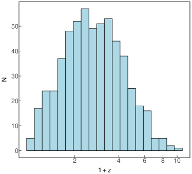
Fig. Set1. Distributions for every parameter

4.2 scatter plots between two arbitrary parameters

We plotted the scatter plots between two arbitrary parameters when the points is not less than 5. We can find that, with this large samples, we can also keep the relationships that found before. We removed the spectral lag value of GRB 060218, because it is an outlier (Foley et al., 2008). The two results are shown in Figure 2. We also made figure set for all the scatter plots. In total there are 1468 plots.

Figure 2: Scatter plots for two arbitrary parameters. One can see all the 1468 plots in Figure. Set 2 . The description of every parameter is defined in Section 2.

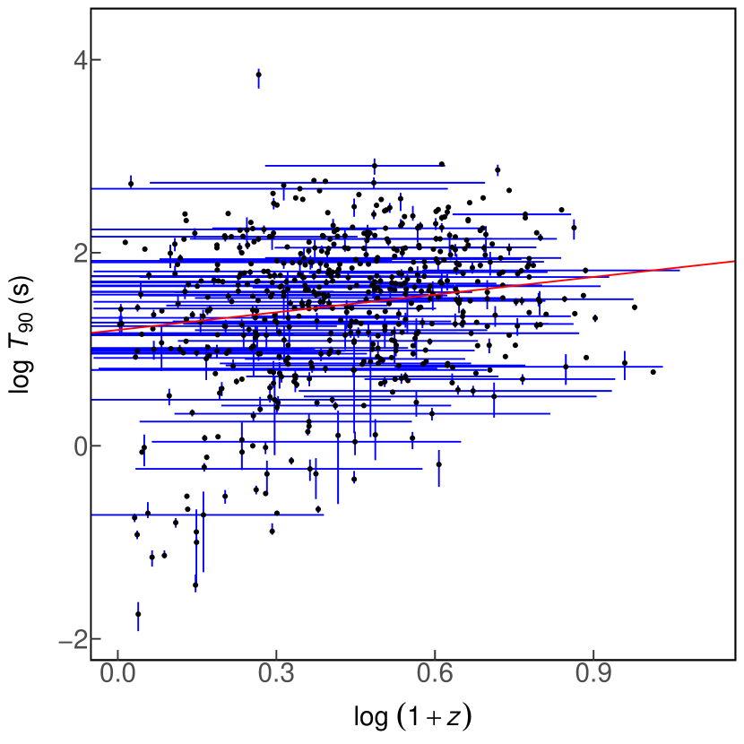
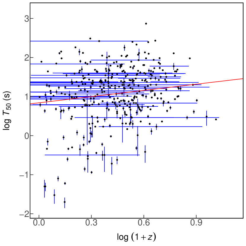
Fig. Set2. Scatter plots for two arbitrary parameters

4.3 Correlation coefficients

Correlation coefficient is to measure the correlation between two parameters, there are 4 methods:

1. $\rm Pearson$ correlation coefficient (Pearson, 1895). Supposed the two variables are $x_{\rm t}$ and $y_{\rm t}$.

   $$\gamma=\frac{\sum_{t=1}^{N}(x_{\rm t}-\bar{x})(y_{\rm t}-\bar{y})}{\sqrt{\sum_{t=1}^{N}(x_{\rm t}-\bar{x})^{2}}\sqrt{\sum_{t=1}^{N}(y_{\rm t}-\bar{y})^{2}}},$$ (5)

   where $\bar{x}$ is the mean of variable $x$, $\bar{y}$ is the mean of variable $y$. $\rm Pearson$ correlation coefficient is based on normal distribution, so when the data is normal distribution, the $\rm Pearson$ correlation coefficient works very well.

2. $\rm Spearman$ correlation coefficient (Spearman, 1987). This coefficient does not depend on the data distribution. It is a kind of rank measure.

   $$\rho=\frac{n(\sum_{t=1}^{N}x_{\rm t}y_{\rm t})-(\sum_{t=1}^{N}x_{\rm t})(\sum_{t=1}^{N}y_{\rm t})}{\sqrt{n(\sum_{t=1}^{N}x_{\rm t}^{2})-(\sum_{t=1}^{N}x_{\rm t})^{2}}\sqrt{n(\sum_{t=1}^{N}y_{\rm t}^{2})-(\sum_{t=1}^{N}y_{\rm t})^{2}}},$$ (6)

3. $\rm Kendall$ $\tau$ correlation coefficient (Kendall, 1938). This coefficient compares the order of the two variables, not comparing the values. It is also a kind of rank measure.

   $$\tau=\frac{n_{\rm c}-n_{\rm d}}{1/2n(n-1)},$$ (7)

   where $n$ is the length of the two variables, $n_{\rm c}$ is the number of concordant pairs, $n_{\rm d}$ is the number of discordant pairs.

4. Cosine similarity (van Dongen & Enright, 2012). Supposed the two variables are $x_{\rm t}$ and $y_{\rm t}$, the cosine similarity definition is

   $$cos\theta_{\rm x,y}=\frac{\sum_{t=1}^{N}x_{\rm t}y_{\rm t}}{\sqrt{\sum_{t=1}^{N}x_{\rm t}^{2}\sum_{t=1}^{N}y_{\rm t}^{2}}},$$ (8)

   when $cos\theta_{\rm x,y}=1$, it means $x_{\rm t}$ and $y_{\rm t}$ are completely similar, when $cos\theta_{\rm x,y}$ is more close to 1, the two variables are more similar.

4.4 Correlation ratio

Pearson correlation coefficients measure the linear correlation between two variables. But when coming to nonlinear correlation, correlation coefficients do not work well. So we need correlation ratio (Fisher, 1970) to measure the nonlinear correlation between different variables. Correlation ratio is a ratio of the statistical dispersion within individual categories and the dispersion across the whole population or sample, defined as the ratio of the standard deviation of within individual categories and the standard deviation of the the whole population or sample.

Supposed the variables is $y_{\rm xi}$, x means the category, i means the $ith$ value for category x, the number of category x is $n_{\rm x}$,

$$\bar{y}_{\rm x}=\frac{\sum_{\rm i}y_{\rm xi}}{n_{\rm x}},$$ (9)

$$\bar{y}=\frac{\sum_{\rm x}n_{\rm x}\bar{y}_{\rm x}}{\sum_{\rm x}n_{\rm x}},$$ (10)

where $\bar{y}_{\rm x}$ is the mean of category x, $\bar{y}$ is the mean of the whole sample, the definition of correlation ratio $\eta$ is

$$\eta^{2}=\frac{\sum_{\rm x}n_{\rm x}(\bar{y}_{\rm x}-\bar{y})^{2}}{\sum_{\rm x,i}(y_{\rm xi}-\bar{y})^{2}},$$ (11)

it is the ratio of the weighted variance of the category means and the variance of the whole sample. $\eta$ is a value between 0 and 1, when $\eta$ is more close to 1, the nonlinear correlation is stronger.

When the two parameters have at least 5 GRBs, then we gave the correlation coefficients and correlation ratio, and we excluded some trivial results. It means we removed the correlations between the rest-frame and observer-frame for the same parameters, like the correlation between $T_{\rm 90}$ and $T_{\rm 90,i}$. We have many results, so we just put the first 5 results in Table 3. One can find all the results in machine readable table. In Table 3, we gave the results of Pearson, Spearman, Kendall $\tau$ coefficients and the related p-values. We also considered all the error bars using MC method (Zou et al., 2018). The last two rows are correlation ratio and cosine similarity with error bars, also using MC method. We did the statistics between two arbitrary parameters in order to find the remarkable correlations. In Section 5, we analyzed some interesting results, and gave some reasonable physical explanations. In this paper, we just analyzed the linear correlations. During all the analysis, Pearson, Spearman, Kendall $\tau$ coefficients and the related p-values are the most important references of linear correlations. When the hypothesis testing p-value is smaller than 0.1, it means the correlation has very high probability to be true. The sample selection biases is quite complicated (see for examples of the related discussion, (Lloyd & Petrosian, 1999; Lloyd et al., 2000a; Dainotti et al., 2013b, 2015a, 2015b)). One should be caution when considering the results. When the absolute values of Pearson, Spearman, Kendall $\tau$ coefficients are bigger, the correlation is stronger. For cosine similarity, there is no hypothesis testing, so it is just used to confirm the linear correlations. For correlation ratio, we will analyzed the nonlinear correlations in the future with this value.

4.5 Linear regression of two parameters and three parameters

We did the linear regression between two parameters and three parameters arbitrarily when the sample number is not smaller than 5. We also considered all the error bars using MC method (Zou et al., 2018). We excluded some trivial results. As an example, the first 5 linear regression results are shown in Table 4 and Table 5, respectively. The full linear regression results are given in two machine readable tables.

In Table 4, $y$ is dependent variable, $x$ is independent variable, $b$ is the intercept of the linear model, and $a$ is the linear coefficient of $x$. Adjusted $R^{2}$ is used to measure the goodness of the regression model. It means the percentage of variance explained considering the parameter freedom. We use the adjusted $R^{2}$ calculated with central values for representation. Because every time of MC, adjusted $R^{2}$ does not change too much. In Table 5, $x_{1}$ and $x_{2}$ are independent variables, $a_{1}$ and $a_{2}$ are the linear coefficients of $x_{1}$ and $x_{2}$ respectively. $y$, $b$ and adjusted $R^{2}$ are same meanings as in Table 4. Readers can see Hron et al. (2012) for more details about linear regression.

5 Remarkable results between two parameters

In this section, we show some remarkable correlations between two parameters. The strategy of choosing the results are the following. The correlation should have at least 10 GRBs. Adjusted $R^{2}$ should be bigger than 0.2 except Section 5.1. The whole linear model and $a$ have hypothesis testing p-values smaller than 0.05. Pearson, Spearman, Kendall $\tau$ coefficients have at least one hypothesis testing p-value smaller than 0.1. For peak energy flux $F_{\rm pk}$ and peak photon flux $P_{\rm pk}$, both of them have four different time bins. If $F_{\rm pk}$ in all the four time bins correlates with another one same parameter, we just showed the best time bin result. The best time bin result has biggest adjusted $R^{2}$. $P_{\rm pk}$ is the same. Other results are all in machine readable tables. Since some relations have been discovered before, we compared the differences between the current and previous analysis. Readers can also see Table 6 for a clear comparison. We just show a part of results in the paper. We provide all the results with figure sets and machine readable tables including our original data. If readers want to analyze with other statistical methods, they can use our original data in machine readable table. One may notice that not only the correlations, but the non-existence of correlations among a certain quantities may also reveal underlying physics of GRBs.

5.1 Some interesting breaks

Interestingly, we found there is a break in the $\log F_{\rm pk}$ and $(-\alpha_{\rm spl})$ plots for all 4 time bins.

The correlation between $\log F_{\rm pk1}$ and $(-\alpha_{\rm spl})$ is:

$$\log F_{\rm pk1}=(-0.75\pm 0.046)\times(-\alpha_{\rm spl})+(1.1\pm 0.083),$$ (12)

where $F_{\rm pk1}$ is peak energy flux of 1 $\rm s$ time bin in rest-frame 1-$10^{4}$ $\rm keV$ energy band and in unit of $\rm 10^{\rm-6}~{}ergs~{}cm^{\rm-2}~{}s^{\rm-1}$. The adjusted $R^{2}$ is 0.3. The Pearson coefficient is $-0.47\pm 0.028$ with p-value $4.2\times 10^{-22}$. The Spearman coefficient is $-0.49\pm 0.024$ with p-value $5.8\times 10^{-25}$. The Kendall $\tau$ coefficient is $-0.34\pm 0.018$ with p-value $7.3\times 10^{-24}$. The correlation ratio is $0.86\pm 0.0037$. The cosine similarity is $-0.37\pm 0.013$. The scatter plot is in Figure 3 . The GRB sample number is 385.

The correlation between $\log F_{\rm pk2}$ and $(-\alpha_{\rm spl})$ is:

$$\log F_{\rm pk2}=(-0.46\pm 0.036)\times(-\alpha_{\rm spl})+(1.1\pm 0.063),$$ (13)

where $F_{\rm pk2}$ is peak energy flux of 64 $\rm ms$ time bin in rest-frame 1-$10^{4}$ $\rm keV$ energy band and in unit of $\rm 10^{\rm-6}~{}ergs~{}cm^{\rm-2}~{}s^{\rm-1}$. The adjusted $R^{2}$ is 0.21. The Pearson coefficient is $-0.37\pm 0.03$ with p-value $1.8\times 10^{-17}$. The Spearman coefficient is $-0.55\pm 0.023$ with p-value $8.8\times 10^{-41}$. The Kendall $\tau$ coefficient is $-0.39\pm 0.018$ with p-value $3.2\times 10^{-38}$. The correlation ratio is $0.81\pm 0.0045$. The cosine similarity is $0.5\pm 0.018$. The scatter plot is in Figure 4. The GRB sample number is 490.

The correlation between $\log F_{\rm pk3}$ and $(-\alpha_{\rm spl})$ is:

$$\log F_{\rm pk3}=(-0.37\pm 0.032)\times(-\alpha_{\rm spl})+(0.84\pm 0.057),$$ (14)

where $F_{\rm pk3}$ is peak energy flux of 256 $\rm ms$ time bin in rest-frame 1-$10^{4}$ $\rm keV$ energy band and in unit of $\rm 10^{\rm-6}~{}ergs~{}cm^{\rm-2}~{}s^{\rm-1}$. The adjusted $R^{2}$ is 0.17. The Pearson coefficient is $-0.33\pm 0.031$ with p-value $4.1\times 10^{-14}$. The Spearman coefficient is $-0.54\pm 0.024$ with p-value $1.6\times 10^{-37}$. The Kendall $\tau$ coefficient is $-0.38\pm 0.018$ with p-value $6.7\times 10^{-36}$. The correlation ratio is $0.85\pm 0.0038$. The cosine similarity is $0.33\pm 0.021$. The scatter plot is in Figure 5. The GRB sample number is 487.

The correlation between $\log F_{\rm pk4}$ and $(-\alpha_{\rm spl})$ is:

$$\log F_{\rm pk4}=(-0.18\pm 0.033)\times(-\alpha_{\rm spl})+(0.22\pm 0.059),$$ (15)

where $F_{\rm pk4}$ is peak energy flux of 1024 $\rm ms$ time bin in rest-frame 1-$10^{4}$ $\rm keV$ energy band and in unit of $\rm 10^{\rm-6}~{}ergs~{}cm^{\rm-2}~{}s^{\rm-1}$. The adjusted $R^{2}$ is 0.055. The Pearson coefficient is $-0.16\pm 0.032$ with p-value $3.4\times 10^{-4}$. The Spearman coefficient is $-0.39\pm 0.027$ with p-value $3.3\times 10^{-19}$. The Kendall $\tau$ coefficient is $-0.28\pm 0.02$ with p-value $1.3\times 10^{-19}$. The correlation ratio is $0.89\pm 0.004$. The cosine similarity is $-0.19\pm 0.018$. The scatter plot is in Figure 6. The GRB sample number is 483.

We also found there is a break in $\log HR$-$\log F_{\rm pk2}$-$(-\alpha_{\rm spl})$ plot. In other three time bins of $F_{\rm pk}$, there are also breaks. We just show the best one.

The $\log HR$-$\log F_{\rm pk2}$-$(-\alpha_{\rm spl})$ relation is:

$$\log HR=(0.17\pm 0.036)\times\log F_{\rm pk2}+(-0.9\pm 0.039)\times(-\alpha_{\rm spl})+(2.2\pm 0.075),$$ (16)

where $F_{\rm pk2}$ is peak energy flux of 64 $\rm ms$ time bin in rest-frame 1-$10^{4}$ $\rm keV$ energy band and in unit of $\rm 10^{\rm-6}~{}ergs~{}cm^{\rm-2}~{}s^{\rm-1}$. The adjusted $R^{2}$ is 0.57. One can see 85 for the scatter plot between these three parameters. The GRB sample number is 490.

It is not clear what causes these breaks. There is also weak signals in $P_{\rm pk}-\alpha_{\rm spl}$ plot. It might be a selection effect, as there is no such effect in $L_{\rm pk}-\alpha_{\rm spl}$ plot or in $F_{\rm g}-\alpha_{\rm spl}$ plot. All the corresponding figures can be found in the figure sets.

5.2 Amati relation

Amati relation (Amati et al., 2002, 2008) is a widely known relation of GRBs.

The correlation between $\log E_{\rm p,band}$ and $\log E_{\rm iso}$ is:

$$\log E_{\rm p,band}=(0.24\pm 0.011)\times\log E_{\rm iso}+(1.9\pm 0.017),$$ (17)

where $E_{\rm p,band}$ is in unit of $\rm keV$, $E_{\rm iso}$ is in unit of $\rm 10^{\rm 52}~{}ergs$ and in rest-frame 1-$10^{4}$ $\rm keV$ energy band. In Amati et al. (2002) initial data, the slope is $0.52\pm 0.06$ with 12 GRBs. Here we have 180 GRBs. The adjusted $R^{2}$ is 0.26. The Pearson coefficient is $0.5\pm 0.021$ with p-value $8.2\times 10^{-13}$. The Spearman coefficient is $0.56\pm 0.019$ with p-value $5.2\times 10^{-16}$. The Kendall $\tau$ coefficient is $0.41\pm 0.014$ with p-value $2.1\times 10^{-16}$. The correlation ratio is $0.62\pm 0.0049$. The cosine similarity is $0.75\pm 0.0055$. It is maybe due to larger $\Gamma_{0}$ in GRBs also have larger energy and peak energy (Ghirlanda et al., 2012), or an optically thin synchrotron shock model (Lloyd et al., 2000b). One can see Section 5.6, $E_{\rm iso}$ and peak energy both correlate with $\Gamma_{0}$. The scatter plot is in Figure 7. The GRB sample number is 180.

The correlation between $\log E_{\rm p,band,i}$ and $\log E_{\rm iso}$ is:

$$\log E_{\rm p,band,i}=(0.35\pm 0.011)\times\log E_{\rm iso}+(2.3\pm 0.018),$$ (18)

In Amati et al. (2008), the slope is $0.57\pm 0.01$ with 70 LGRBs and X-ray flares. We have 178 GRBs. where $E_{\rm p,band,i}$ is in unit of $\rm keV$. $E_{\rm iso}$ is in unit of $\rm 10^{\rm 52}~{}ergs$ and in rest-frame 1-$10^{4}$ $\rm keV$ energy band. The adjusted $R^{2}$ is 0.45. The Pearson coefficient is $0.65\pm 0.019$ with p-value $7.2\times 10^{-23}$. The Spearman coefficient is $0.69\pm 0.018$ with p-value $4.9\times 10^{-26}$. The Kendall $\tau$ coefficient is $0.51\pm 0.015$ with p-value $3.1\times 10^{-24}$. The correlation ratio is $0.72\pm 0.0038$. The cosine similarity is $0.78\pm 0.0052$. The scatter plot is in Figure 8. The GRB sample number is 178. The better correlation between $\log E_{\rm p,band,i}$ and $\log E_{\rm iso}$ comparing with $\log E_{\rm p,band}$ and $\log E_{\rm iso}$ suggests this correlation is intrinsic. With enough data, one would investigate this relation within subgroups (Zhang et al., 2009b; Qin & Chen, 2013; Zou et al., 2018). A previous study gave $E_{\rm iso}=10^{53.00\pm 0.045}\times[\frac{E_{\rm p,band,i}}{355keV}]^{1.57\pm 0.099}$ with 101 samples (Yonetoku et al., 2010), and $\log(\frac{E_{\rm iso}}{1erg})=1.75^{+0.18}_{-0.16}\times\log[\frac{E_{\rm p,band,i}}{300keV}]+(52.53\pm 0.02)$ with 162 samples (Demianski et al., 2017).

5.3 Some correlations about $L_{\rm pk}$

5.3.1 Yonetoku relation

Yonetoku et al. (2004) found the correlation between rest-frame peak energy and peak luminosity. We also did the correlations of $\log E_{\rm p,band}$ - $\log L_{\rm pk}$ and $\log E_{\rm p,band,i}$ - $\log L_{\rm pk}$.

The correlation between $\log L_{\rm pk}$ and $\log E_{\rm p,band}$ is:

$$\log L_{\rm pk}=(1\pm 0.061)\times\log E_{\rm p,band}+(-2\pm 0.13),$$ (19)

where $L_{\rm pk}$ is in unit of $\rm 10^{\rm 52}~{}erg~{}s^{\rm-1}$ and in 1-$10^{4}$ $\rm keV$ energy band. $E_{\rm p,band}$ is in unit of $\rm keV$. The adjusted $R^{2}$ is 0.25. The Pearson coefficient is $0.49\pm 0.022$ with p-value $3.2\times 10^{-9}$. The Spearman coefficient is $0.52\pm 0.025$ with p-value $1.5\times 10^{-10}$. The Kendall $\tau$ coefficient is $0.37\pm 0.019$ with p-value $4.9\times 10^{-10}$. The correlation ratio is $0.8\pm 0.004$. The cosine similarity is $0.33\pm 0.014$. The scatter plot is in Figure 10. The GRB sample number is 130.

The correlation between $\log L_{\rm pk}$ and $\log E_{\rm p,band,i}$ is:

$$\log L_{\rm pk}=(1.2\pm 0.055)\times\log E_{\rm p,band,i}+(-2.9\pm 0.14),$$ (20)

In Yonetoku et al. (2004), the slope is $1.94\pm 0.19$ with 11 samples. where $L_{\rm pk}$ is in unit of $\rm 10^{\rm 52}~{}erg~{}s^{\rm-1}$ and in 1-$10^{4}$ $\rm keV$ energy band. $E_{\rm p,band,i}$ is in unit of $\rm keV$. The adjusted $R^{2}$ is 0.42. The Pearson coefficient is $0.63\pm 0.019$ with p-value $4\times 10^{-15}$. The Spearman coefficient is $0.64\pm 0.025$ with p-value $4.3\times 10^{-16}$. The Kendall $\tau$ coefficient is $0.47\pm 0.019$ with p-value $7.5\times 10^{-15}$. The correlation ratio is $0.85\pm 0.0031$. The cosine similarity is $0.34\pm 0.013$. The scatter plot is in Figure 9. The GRB sample number is 127. The rest frame peak energy is also better correlated with the luminosity. Yonetoku et al. (2010) reanalyzed 101 GRBs, and examined how the truncation of the detector sensitivity affects the Amati and Yonetoku relations. They conclude they are surely intrinsic properties of GRBs. The result of Yonetoku et al. (2010) is $L_{\rm pk}=10^{52.43\pm 0.037}\times[\frac{E_{\rm p,band,i}}{355keV}]^{1.60\pm 0.082}$ with 101 samples.

5.3.2 Other correlations about $L_{\rm pk}$

The correlation between $\log L_{\rm pk}$ and $\log offset$ is:

$$\log L_{\rm pk}=(-0.68\pm 0.24)\times\log offset+(-0.047\pm 0.15),$$ (21)

where $L_{\rm pk}$ is in unit of $\rm 10^{\rm 52}~{}erg~{}s^{\rm-1}$ and in 1-$10^{4}$ $\rm keV$ energy band. Host galaxy offset is in unit of $\rm kpc$. The adjusted $R^{2}$ is 0.22. The Pearson coefficient is $-0.42\pm 0.092$ with p-value $3\times 10^{-2}$. The Spearman coefficient is $-0.44\pm 0.041$ with p-value $2.2\times 10^{-2}$. The Kendall $\tau$ coefficient is $-0.31\pm 0.035$ with p-value $2.3\times 10^{-2}$. The correlation ratio is $0.42\pm 0.043$. The cosine similarity is $-0.5\pm 0.085$. The scatter plot is in Figure 11. The GRB sample number is 27. As the short GRBs locate in the outer regions of the host galaxies, and they are less luminous, this may cause the anti-correlation between $L_{\rm pk}$ and the offset.

The correlation between $\log L_{\rm pk}$ and $\log t_{\rm pkOpt}$ is:

$$\log L_{\rm pk}=(-0.74\pm 0.04)\times\log t_{\rm pkOpt}+(1.9\pm 0.092),$$ (22)

where $L_{\rm pk}$ is in unit of $\rm 10^{\rm 52}~{}erg~{}s^{\rm-1}$ and in 1-$10^{4}$ $\rm keV$ energy band. $t_{\rm pkOpt}$ is in unit of $\rm s$. The adjusted $R^{2}$ is 0.26. The Pearson coefficient is $-0.51\pm 0.023$ with p-value $1.5\times 10^{-6}$. The Spearman coefficient is $-0.39\pm 0.033$ with p-value $3.5\times 10^{-4}$. The Kendall $\tau$ coefficient is $-0.27\pm 0.024$ with p-value $4\times 10^{-4}$. The correlation ratio is $0.84\pm 0.0038$. The cosine similarity is $-0.067\pm 0.026$. The scatter plot is in Figure 13. The GRB sample number is 80.

The correlation between $\log L_{\rm pk}$ and $\log t_{\rm pkOpt,i}$ is:

$$\log L_{\rm pk}=(-0.87\pm 0.036)\times\log t_{\rm pkOpt,i}+(1.8\pm 0.069),$$ (23)

where $L_{\rm pk}$ is in unit of $\rm 10^{\rm 52}~{}erg~{}s^{\rm-1}$ and in 1-$10^{4}$ $\rm keV$ energy band. $t_{\rm pkOpt,i}$ is in unit of $\rm s$. The adjusted $R^{2}$ is 0.4. The Pearson coefficient is $-0.62\pm 0.019$ with p-value $1.1\times 10^{-9}$. The Spearman coefficient is $-0.48\pm 0.031$ with p-value $5.6\times 10^{-6}$. The Kendall $\tau$ coefficient is $-0.33\pm 0.023$ with p-value $1.3\times 10^{-5}$. The correlation ratio is $0.78\pm 0.0049$. The cosine similarity is $-0.13\pm 0.025$. The scatter plot is in Figure 12. The GRB sample number is 80. This anti-correlation is mainly caused by the Lorentz factor, of which higher Lorentz factor corresponds to shorter deceleration time, and consequently smaller $t_{\rm pkOpt,i}$. We can also see the rest frame peak time is better correlated with the luminosity than the observational peak time.

5.4 Some correlations about host galaxy

We found there are some correlations between host galaxy parameters and redshift, also $D_{\rm L}$. Especially Mag has correlations with many parameters.

5.4.1 Some correlations about Mag and other parameters

The correlation between Mag and $\log Mass$ is:

$$Mag=(-1.8\pm 0.34)\times\log Mass+(-4\pm 3.3),$$ (24)

where Mass is in unit of $M_{\bigodot}$, and Mag is in unit of magnitude. The adjusted $R^{2}$ is 0.84. The Pearson coefficient is $-0.48\pm 0.077$ with p-value $4.2\times 10^{-6}$. The Spearman coefficient is $-0.45\pm 0.083$ with p-value $1.8\times 10^{-5}$. The Kendall $\tau$ coefficient is $-0.32\pm 0.061$ with p-value $2.5\times 10^{-5}$. The correlation ratio is $0.99\pm 0.00099$. The cosine similarity is $-0.99\pm 0.00091$. The scatter plot is in Figure 14. The GRB sample number is 82. The luminosity of the host galaxy is positively related with its mass. It might be worthy to investigate the correlations for different types of galaxies, such as host galaxies of GRBs, of supernovae, radio load galaxies etc.

The correlation between Mag and $\log SFR$ is:

$$Mag=(-1.8\pm 0.41)\times\log SFR+(-19\pm 0.51),$$ (25)

where SFR is in unit of $\rm M_{\bigodot}~{}yr^{\rm-1}$. Mag is in unit of magnitude. The adjusted $R^{2}$ is 0.78. The Pearson coefficient is $-0.56\pm 0.1$ with p-value $7.1\times 10^{-4}$. The Spearman coefficient is $-0.5\pm 0.12$ with p-value $3.1\times 10^{-3}$. The Kendall $\tau$ coefficient is $-0.36\pm 0.091$ with p-value $3.6\times 10^{-3}$. The correlation ratio is $0.98\pm 0.0032$. The cosine similarity is $-0.78\pm 0.027$. The scatter plot is in Figure 15. The GRB sample number is 33. It might be more interesting to get the correlations for the specific SFR. However, those correlations are not obvious enough.

The correlation between Mag and metallicity is:

$$Mag=(-3.4\pm 1.6)\times metallicity+(8.4\pm 14),$$ (26)

where Mag is in unit of magnitude. Metallicity is the value of $12+\log O/H$. The adjusted $R^{2}$ is 0.41. The Pearson coefficient is $-0.42\pm 0.15$ with p-value $7.4\times 10^{-2}$. The Spearman coefficient is $-0.41\pm 0.17$ with p-value $7.8\times 10^{-2}$. The Kendall $\tau$ coefficient is $-0.29\pm 0.13$ with p-value $7.4\times 10^{-2}$. The correlation ratio is $0.99\pm 0.0025$. The cosine similarity is $-0.99\pm 0.0022$. The scatter plot is in Figure 16. The GRB sample number is 19. Metallicity indicates the star formation properties, and consequently the information of the progenitors of GRBs. However, the sample is not big enough, and the correlation is not very tight. One may not find much information from this correlation right now.

The correlation between Mag and $\log F_{\rm Opt11hr}$ is:

$$Mag=(0.73\pm 0.3)\times\log F_{\rm Opt11hr}+(-17\pm 1.5),$$ (27)

where $F_{\rm Opt11hr}$ is in unit of $\rm Jy$. Mag is in unit of magnitude. The adjusted $R^{2}$ is 0.27. The Pearson coefficient is $0.27\pm 0.1$ with p-value $3.3\times 10^{-2}$. The Spearman coefficient is $0.23\pm 0.11$ with p-value $7.3\times 10^{-2}$. The Kendall $\tau$ coefficient is $0.16\pm 0.075$ with p-value $6.9\times 10^{-2}$. The correlation ratio is $0.97\pm 0.004$. The cosine similarity is $0.98\pm 0.0028$. The scatter plot is in Figure 17. The GRB sample number is 64. It is interesting that the magnitude of the host galaxy is related to the observed flux density of the afterglow. It is probably that the number density of the smaller galaxy is higher, and the luminosity at 11 hour is brighter.

The correlation between Mag and $\log D_{\rm L}$ is:

$$Mag=(-1.9\pm 0.53)\times\log D_{\rm L}+(-20\pm 0.37),$$ (28)

where $D_{\rm L}$ is in unit of $\rm 10^{\rm 28}~{}cm$. Mag is in unit of magnitude. The adjusted $R^{2}$ is 0.26. The Pearson coefficient is $-0.3\pm 0.081$ with p-value $6.9\times 10^{-3}$. The Spearman coefficient is $-0.2\pm 0.091$ with p-value $7.5\times 10^{-2}$. The Kendall $\tau$ coefficient is $-0.14\pm 0.064$ with p-value $7.3\times 10^{-2}$. The correlation ratio is $0.99\pm 0.002$. The cosine similarity is $-0.82\pm 0.0058$. The scatter plot is in Figure 18. The GRB sample number is 81. This relation shows the observational selection effect on the data. Because of the flux limit of the observations, only bright galaxies can be observed in the far distance. The observed host galaxies is correlated to the distance.

5.4.2 Some other correlations between parameters related to host galaxies

The correlation between metallicity and $\log Mass$ is:

$$metallicity=(0.19\pm 0.025)\times\log Mass+(6.8\pm 0.24),$$ (29)

where metallicity is the value of $12+\log O/H$. Mass is in unit of $M_{\bigodot}$. The adjusted $R^{2}$ is 0.3. The Pearson coefficient is $0.47\pm 0.054$ with p-value $9.3\times 10^{-5}$. The Spearman coefficient is $0.49\pm 0.057$ with p-value $3.7\times 10^{-5}$. The Kendall $\tau$ coefficient is $0.34\pm 0.043$ with p-value $6.7\times 10^{-5}$. The correlation ratio is $0.54\pm 0.022$. The cosine similarity is $1\pm 0.00033$. The scatter plot is in Figure 19. The GRB sample number is 64. The metallicity is positively correlated with the mass, which may indicate the history of merging of the galaxies. Arabsalmani et al. (2018) studied the mass-metallicity relation for GRB host galaxies, and found GRB-selected galaxies appear to track the mass-metallicity relation of star forming galaxies but with an offset of 0.15 towards lower metallicities.

The correlation between $\log SFR$ and $\log(1+z)$ is:

$$\log SFR=(4.1\pm 0.19)\times\log(1+z)+(-0.59\pm 0.051),$$ (30)

where SFR is in unit of $\rm M_{\bigodot}~{}yr^{\rm-1}$. The adjusted $R^{2}$ is 0.49. The Pearson coefficient is $0.69\pm 0.019$ with p-value $1.3\times 10^{-14}$. The Spearman coefficient is $0.69\pm 0.02$ with p-value $4.8\times 10^{-15}$. The Kendall $\tau$ coefficient is $0.49\pm 0.018$ with p-value $1.6\times 10^{-12}$. The correlation ratio is $0.24\pm 0.018$. The cosine similarity is $0.76\pm 0.016$. The scatter plot is in Figure 20. The GRB sample number is 96. This relation may indicate the history of the star formation. However, one should be caution about the data selection effect.

The correlation between $\log SFR$ and $\log D_{\rm L}$ is:

$$\log SFR=(1.2\pm 0.047)\times\log D_{\rm L}+(0.43\pm 0.025),$$ (31)

where SFR is in unit of $\rm M_{\bigodot}~{}yr^{\rm-1}$. $D_{\rm L}$ is in unit of $\rm 10^{\rm 28}~{}cm$. The adjusted $R^{2}$ is 0.42. The Pearson coefficient is $0.64\pm 0.018$ with p-value $3.2\times 10^{-12}$. The Spearman coefficient is $0.66\pm 0.021$ with p-value $2.1\times 10^{-13}$. The Kendall $\tau$ coefficient is $0.46\pm 0.019$ with p-value $2.1\times 10^{-11}$. The correlation ratio is $0.29\pm 0.016$. The cosine similarity is $0.69\pm 0.014$. The scatter plot is in Figure 21. The GRB sample number is 96. This is similar to the ${\rm SFR}$ and $(1+z)$ relation.

The correlation between $\log Mass$ and $\log SFR$ is:

$$\log Mass=(0.62\pm 0.041)\times\log SFR+(9.1\pm 0.046),$$ (32)

where mass is in unit of $M_{\bigodot}$. SFR is in unit of $\rm M_{\bigodot}~{}yr^{\rm-1}$. The adjusted $R^{2}$ is 0.54. The Pearson coefficient is $0.69\pm 0.034$ with p-value $5.2\times 10^{-11}$. The Spearman coefficient is $0.71\pm 0.034$ with p-value $9.6\times 10^{-12}$. The Kendall $\tau$ coefficient is $0.52\pm 0.032$ with p-value $2\times 10^{-10}$. The correlation ratio is $0.98\pm 0.0011$. The cosine similarity is $0.57\pm 0.021$. The scatter plot is in Figure 22. The GRB sample number is 69. It is natural that the more massive galaxy has more intense total star formation rate. Notice the index is $0.62\pm 0.041$, which means the less massive galaxies is more effeminate for the star forming per unit mass.

The correlation between $\log F_{\rm Opt11hr}$ and $\log SFR$ is:

$$\log F_{\rm Opt11hr}=(-0.44\pm 0.073)\times\log SFR+(-4.6\pm 0.074),$$ (33)

where $F_{\rm Opt11hr}$ is in unit of $\rm Jy$. SFR is in unit of $\rm M_{\bigodot}~{}yr^{\rm-1}$. The adjusted $R^{2}$ is 0.24. The Pearson coefficient is $-0.43\pm 0.065$ with p-value $1.7\times 10^{-3}$. The Spearman coefficient is $-0.43\pm 0.069$ with p-value $1.6\times 10^{-3}$. The Kendall $\tau$ coefficient is $-0.29\pm 0.051$ with p-value $2.3\times 10^{-3}$. The correlation ratio is $0.94\pm 0.0042$. The cosine similarity is $-0.57\pm 0.03$. The scatter plot is in Figure 23. The GRB sample number is 51. This correlation is related to the correlations in eq. (32) and in eq. (27).

The correlation between $\log Age$ and $\log E_{\rm p,cpl}$ is:

$$\log Age=(-0.69\pm 0.19)\times\log E_{\rm p,cpl}+(4.3\pm 0.47),$$ (34)

where $E_{\rm p,cpl}$ is in unit of $\rm keV$. Age is in unit of $\rm Myr$. The adjusted $R^{2}$ is 0.24. The Pearson coefficient is $-0.39\pm 0.1$ with p-value $2.2\times 10^{-2}$. The Spearman coefficient is $-0.39\pm 0.11$ with p-value $1.9\times 10^{-2}$. The Kendall $\tau$ coefficient is $-0.27\pm 0.077$ with p-value $2.1\times 10^{-2}$. The correlation ratio is $0.24\pm 0.049$. The cosine similarity is $0.92\pm 0.0086$. The scatter plot is in Figure 42. The GRB sample number is 35.

The correlation between $\log Age$ and $\log E_{\rm p,cpl,i}$ is:

$$\log Age=(-0.81\pm 0.16)\times\log E_{\rm p,cpl,i}+(4.8\pm 0.43),$$ (35)

where Age is in unit of $\rm Myr$. $E_{\rm p,cpl,i}$ is in unit of $\rm keV$. The adjusted $R^{2}$ is 0.39. The Pearson coefficient is $-0.5\pm 0.087$ with p-value $2.1\times 10^{-3}$. The Spearman coefficient is $-0.51\pm 0.094$ with p-value $1.8\times 10^{-3}$. The Kendall $\tau$ coefficient is $-0.36\pm 0.071$ with p-value $2.3\times 10^{-3}$. The correlation ratio is $0.069\pm 0.042$. The cosine similarity is $0.91\pm 0.0086$. The scatter plot is in Figure 43. The GRB sample number is 35. This interesting correlation might be an counter evidence for the two origins of the GRBs. Short GRBs are from merger of double compact objects, which needs longer time of evolution, and consequently in older galaxies. And Short GRBs are harder in spectrum, and the peak energy $E_{\rm p,cpl,i}$ should be higher. Therefore, The age should be positively correlated to the peak energy, while eq. (35) shows it contrarily.

5.5 Correlations about HR

5.5.1 Correlations with HR

The correlation between $(-\alpha_{\rm spl})$ and $\log HR$ is:

$$(-\alpha_{\rm spl})=(-0.55\pm 0.021)\times\log HR+(2.1\pm 0.017),$$ (36)

the adjusted $R^{2}$ is 0.69. The Pearson coefficient is $-0.73\pm 0.016$ with p-value $1.6\times 10^{-148}$. The Spearman coefficient is $-0.78\pm 0.011$ with p-value $1.9\times 10^{-176}$. The Kendall $\tau$ coefficient is $-0.6\pm 0.01$ with p-value $8.4\times 10^{-158}$. The correlation ratio is $0.71\pm 0.0043$. The cosine similarity is $0.59\pm 0.0093$. The scatter plot is in Figure 24. The GRB sample number is 874. This just shows the consistency of the spectrum. The outliers and the width show the hardness ratio itself is not good enough to present the information of the spectrum. All the correlations below in this section show the similar information.

The correlation between $\log E_{\rm p,cpl}$ and $\log HR$ is:

$$\log E_{\rm p,cpl}=(0.54\pm 0.013)\times\log HR+(2.1\pm 0.0084),$$ (37)

where $E_{\rm p,cpl}$ is in unit of $\rm keV$. The adjusted $R^{2}$ is 0.65. The Pearson coefficient is $0.69\pm 0.014$ with p-value $3.8\times 10^{-211}$. The Spearman coefficient is $0.78\pm 0.0094$ with p-value $6.5\times 10^{-305}$. The Kendall $\tau$ coefficient is $0.61\pm 0.0083$ with p-value $1.1\times 10^{-267}$. The correlation ratio is $0.86\pm 0.0023$. The cosine similarity is $0.67\pm 0.008$. The scatter plot is in Figure 25. The GRB sample number is 1469.

The correlation between $\log E_{\rm p,cpl,i}$ and $\log HR$ is:

$$\log E_{\rm p,cpl,i}=(0.55\pm 0.036)\times\log HR+(2.6\pm 0.018),$$ (38)

where $E_{\rm p,cpl,i}$ is in unit of $\rm keV$. The adjusted $R^{2}$ is 0.6. The Pearson coefficient is $0.63\pm 0.03$ with p-value $4.3\times 10^{-27}$. The Spearman coefficient is $0.68\pm 0.028$ with p-value $1.9\times 10^{-32}$. The Kendall $\tau$ coefficient is $0.49\pm 0.023$ with p-value $2.2\times 10^{-28}$. The correlation ratio is $0.93\pm 0.0032$. The cosine similarity is $0.38\pm 0.026$. The scatter plot is in Figure 26. The GRB sample number is 229.

The correlation between $\log E_{\rm p,band}$ and $\log HR$ is:

$$\log E_{\rm p,band}=(0.47\pm 0.017)\times\log HR+(2\pm 0.01),$$ (39)

where $E_{\rm p,band}$ is in unit of $\rm keV$. The adjusted $R^{2}$ is 0.51. The Pearson coefficient is $0.63\pm 0.017$ with p-value $5.2\times 10^{-149}$. The Spearman coefficient is $0.72\pm 0.01$ with p-value $2.3\times 10^{-214}$. The Kendall $\tau$ coefficient is $0.56\pm 0.0081$ with p-value $5.9\times 10^{-207}$. The correlation ratio is $0.9\pm 0.0021$. The cosine similarity is $0.81\pm 0.0079$. The scatter plot is in Figure 27. The GRB sample number is 1332.

The correlation between $\log E_{\rm p,band,i}$ and $\log HR$ is:

$$\log E_{\rm p,band,i}=(0.58\pm 0.066)\times\log HR+(2.4\pm 0.041),$$ (40)

where $E_{\rm p,band,i}$ is in unit of $\rm keV$. The adjusted $R^{2}$ is 0.3. The Pearson coefficient is $0.48\pm 0.045$ with p-value $4.6\times 10^{-9}$. The Spearman coefficient is $0.6\pm 0.035$ with p-value $1.4\times 10^{-14}$. The Kendall $\tau$ coefficient is $0.47\pm 0.028$ with p-value $4\times 10^{-16}$. The correlation ratio is $0.94\pm 0.0025$. The cosine similarity is $0.87\pm 0.013$. The scatter plot is in Figure 28. The GRB sample number is 136.

5.5.2 Correlations between parameters related with HR or peak energies

The correlation between $\log F_{\rm pk1}$ and $\log HR$ is:

$$\log F_{\rm pk1}=(0.6\pm 0.017)\times\log HR+(-0.34\pm 0.0094),$$ (41)

where $F_{\rm pk1}$ is peak energy flux of 1 $\rm s$ time bin in rest-frame 1-$10^{4}$ $\rm keV$ energy band and in unit of $\rm 10^{\rm-6}~{}ergs~{}cm^{\rm-2}~{}s^{\rm-1}$. The adjusted $R^{2}$ is 0.26. The Pearson coefficient is $0.45\pm 0.011$ with p-value $3.9\times 10^{-75}$. The Spearman coefficient is $0.47\pm 0.01$ with p-value $7.9\times 10^{-83}$. The Kendall $\tau$ coefficient is $0.33\pm 0.0073$ with p-value $4.2\times 10^{-79}$. The correlation ratio is $0.37\pm 0.0044$. The cosine similarity is $0.29\pm 0.011$. The scatter plot is in Figure 29. The GRB sample number is 1494. Though there is a correlation, one would say it is just a weak tendency.

In Mallozzi et al. (1995), they found a correlation between mean peak energies and 256 $\rm ms$ peak photon flux $P_{pk2}$. With accumulated more data, we found $P_{pk2}$ and peak energy have no obvious correlation with adjusted $R_{2}$ smaller than 0.1, except $P_{\rm pk4}$ and $E_{\rm p,band}$.

The correlation between $\log E_{\rm p,band}$ and $\log P_{\rm pk4}$ is:

$$\log E_{\rm p,band}=(0.28\pm 0.03)\times\log P_{\rm pk4}+(1.8\pm 0.033),$$ (42)

where $P_{\rm pk4}$ is peak photon flux of 1 $\rm s$ time bin in 10-1000 $\rm keV$ and in unit of $\rm photons~{}cm^{\rm-2}~{}s^{\rm-1}$. $E_{\rm p,band}$ is in unit of $\rm keV$. The adjusted $R^{2}$ is 0.19. The Pearson coefficient is $0.4\pm 0.032$ with p-value $1.9\times 10^{-8}$. The Spearman coefficient is $0.46\pm 0.024$ with p-value $4.5\times 10^{-11}$. The Kendall $\tau$ coefficient is $0.31\pm 0.017$ with p-value $3.4\times 10^{-10}$. The correlation ratio is $0.71\pm 0.0087$. The cosine similarity is $0.81\pm 0.017$. The scatter plot is in Figure 30. The GRB sample number is 181. As one can see it from the figure, even this relation is not very not very tight. One would say there no much correlation between peak energies in spectra and peak photon fluxes in light curves.

Alternatively, we found a more tight correlation between peak energy flux and peak energy. Peak energy flux can be calculated from peak photon flux, so this correlation is natural.

The correlation between $\log E_{\rm p,cpl}$ and $\log F_{\rm pk1}$ is:

$$\log E_{\rm p,cpl}=(0.31\pm 0.012)\times\log F_{\rm pk1}+(2.3\pm 0.0067),$$ (43)

where $F_{\rm pk1}$ is peak energy flux of 1 $\rm s$ time bin in rest-frame 1-$10^{4}$ $\rm keV$ energy band and in unit of $\rm 10^{\rm-6}~{}ergs~{}cm^{\rm-2}~{}s^{\rm-1}$. $E_{\rm p,cpl}$ is in unit of $\rm keV$. The adjusted $R^{2}$ is 0.33. The Pearson coefficient is $0.48\pm 0.018$ with p-value $1.7\times 10^{-43}$. The Spearman coefficient is $0.47\pm 0.018$ with p-value $1.6\times 10^{-42}$. The Kendall $\tau$ coefficient is $0.33\pm 0.013$ with p-value $3.4\times 10^{-42}$. The correlation ratio is $0.9\pm 0.0014$. The cosine similarity is $-0.22\pm 0.0083$. The scatter plot is in Figure 31. The GRB sample number is 749.

The correlation between $\log E_{\rm p,band}$ and $\log F_{\rm pk2}$ is:

$$\log E_{\rm p,band}=(0.28\pm 0.012)\times\log F_{\rm pk2}+(2.2\pm 0.0049),$$ (44)

where $F_{\rm pk2}$ is peak energy flux of 64 $\rm ms$ time bin in rest-frame 1-$10^{4}$ $\rm keV$ energy band and in unit of $\rm 10^{\rm-6}~{}ergs~{}cm^{\rm-2}~{}s^{\rm-1}$. $E_{\rm p,band}$ is in unit of $\rm keV$. The adjusted $R^{2}$ is 0.33. The Pearson coefficient is $0.5\pm 0.015$ with p-value $1.1\times 10^{-73}$. The Spearman coefficient is $0.52\pm 0.012$ with p-value $6.7\times 10^{-81}$. The Kendall $\tau$ coefficient is $0.36\pm 0.009$ with p-value $1.5\times 10^{-75}$. The correlation ratio is $0.89\pm 0.0024$. The cosine similarity is $0.4\pm 0.015$. The scatter plot is in Figure 32. The GRB sample number is 1168. One can see from these two figures, the data are still widely distributed. What’s more, as the flux is the energy of the photons multiplied by the number of the photons, the flux contains the information from the spectrum. Therefore, these two correlations does not reveal more information.

5.6 Correlations about Lorentz factor $\Gamma_{0}$

The correlation between $\log\Gamma_{0}$ and $\log E_{\rm iso}$ is:

$$\log\Gamma_{0}=(0.35\pm 0.014)\times\log E_{\rm iso}+(1.9\pm 0.018),$$ (45)

where $E_{\rm iso}$ is in unit of $\rm 10^{\rm 52}~{}ergs$ and in rest-frame 1-$10^{4}$ $\rm keV$ energy band. The adjusted $R^{2}$ is 0.58. The Pearson coefficient is $0.75\pm 0.016$ with p-value $1.9\times 10^{-10}$. The Spearman coefficient is $0.68\pm 0.02$ with p-value $4.4\times 10^{-8}$. The Kendall $\tau$ coefficient is $0.52\pm 0.019$ with p-value $9.5\times 10^{-8}$. The correlation ratio is $0.67\pm 0.0065$. The cosine similarity is $0.79\pm 0.013$. The scatter plot is in Figure 35. The GRB sample number is 51. Previous studies gave $\log{\Gamma_{\rm 0}}=(0.269\pm 0.002)\log{E_{\rm iso,52}}+(2.291\pm 0.002)$ with 19 samples (Liang et al., 2010) and $\log{\Gamma_{\rm 0}}=(0.29\pm 0.002)\log{E_{\rm iso,52}}+(1.96\pm 0.002)$ with 38 samples (Lü et al., 2012), which are shown here for comparison. The positive correlation shows that the stronger bursts is likely to produce faster ejecta, which might reveals the acceleration mechanism of the central engine.

The correlation between $\log\Gamma_{0}$ and $\log L_{\rm pk}$ is:

$$\log\Gamma_{0}=(0.29\pm 0.011)\times\log L_{\rm pk}+(2.2\pm 0.01),$$ (46)

where $L_{\rm pk}$ is in unit of $\rm 10^{\rm 52}~{}erg~{}s^{\rm-1}$ and in 1-$10^{4}$ $\rm keV$ energy band. The adjusted $R^{2}$ is 0.66. The Pearson coefficient is $0.81\pm 0.015$ with p-value $1.1\times 10^{-10}$. The Spearman coefficient is $0.63\pm 0.031$ with p-value $7\times 10^{-6}$. The Kendall $\tau$ coefficient is $0.47\pm 0.027$ with p-value $1\times 10^{-5}$. The correlation ratio is $0.77\pm 0.0061$. The cosine similarity is $0.16\pm 0.026$. The scatter plot is in Figure 33. The GRB sample number is 42. A previous study gave $\log{\Gamma_{\rm 0}}=(0.28\pm 0.002)\log{L_{\rm iso,52}}+(2.39\pm 0.003)$ with 38 samples (Lü et al., 2012). This correlation is related to eq. (45).

The correlation between $\log\Gamma_{0}$ and $\log t_{\rm pkOpt,i}$ is:

$$\log\Gamma_{0}=(-0.49\pm 0.011)\times\log t_{\rm pkOpt,i}+(3.2\pm 0.026),$$ (47)

where $t_{\rm pkOpt,i}$ is in unit of $\rm s$. The adjusted $R^{2}$ is 0.66. The Pearson coefficient is $-0.81\pm 0.011$ with p-value $1.5\times 10^{-11}$. The Spearman coefficient is $-0.64\pm 0.019$ with p-value $2.6\times 10^{-6}$. The Kendall $\tau$ coefficient is $-0.48\pm 0.019$ with p-value $3.5\times 10^{-6}$. The correlation ratio is $0.019\pm 0.0085$. The cosine similarity is $0.9\pm 0.0016$. The scatter plot is in Figure 34. The GRB sample number is 45. A previous study gave $\log\Gamma_{0}=(-0.63\pm 0.04)\times\log t_{\rm pkOpt,i}+(3.69\pm 0.09)$ with 19 samples (Liang et al., 2010) (Notice two of them are the peak times in X-rays). The anti-correlation mainly reveals how the GRB jets decelerate by the circum burst environment. Noticing the deceleration time is also related to the profile of the density of the environment, the correlation here may not be very tight.

The correlation between $\log\Gamma_{0}$ and $\log t_{\rm pkOpt}$ is:

$$\log\Gamma_{0}=(-0.48\pm 0.012)\times\log t_{\rm pkOpt}+(3.4\pm 0.033),$$ (48)

where $t_{\rm pkOpt}$ is in unit of $\rm s$. The adjusted $R^{2}$ is 0.56. The Pearson coefficient is $-0.75\pm 0.012$ with p-value $3.4\times 10^{-9}$. The Spearman coefficient is $-0.59\pm 0.022$ with p-value $2.4\times 10^{-5}$. The Kendall $\tau$ coefficient is $-0.44\pm 0.021$ with p-value $1.8\times 10^{-5}$. The correlation ratio is $0.38\pm 0.0084$. The cosine similarity is $0.93\pm 0.0012$. The scatter plot is in Figure 36. The GRB sample number is 45. This correlation is clearly worse than the previous one shown in equation 47, which has the redshift correction. It implies the correlation between $\Gamma_{0}$ and $t_{\rm pkOpt,i}$ is intrinsic, and the time dilation due to redshift goes against the correlation.

The correlation between $\log\Gamma_{0}$ and $\log D_{\rm L}$ is:

$$\log\Gamma_{0}=(0.58\pm 0.0095)\times\log D_{\rm L}+(1.9\pm 0.0074),$$ (49)

where $D_{\rm L}$ is in unit of $\rm 10^{\rm 28}~{}cm$. The adjusted $R^{2}$ is 0.43. The Pearson coefficient is $0.67\pm 0.01$ with p-value $2.6\times 10^{-8}$. The Spearman coefficient is $0.5\pm 0.019$ with p-value $9.6\times 10^{-5}$. The Kendall $\tau$ coefficient is $0.35\pm 0.014$ with p-value $1.5\times 10^{-4}$. The correlation ratio is $0.89\pm 0.00096$. The cosine similarity is $0.78\pm 0.0014$. The scatter plot is in Figure 37. The GRB sample number is 55. The dependence on the distance indicates observational bias, that the low $\Gamma_{0}$ GRBs might not be able to be observed at longer distance. The other possibility is that the GRBs exploded earlier do have higher $\Gamma_{0}$.

The correlation between $\log\Gamma_{0}$ and $\log t_{\rm radio,pk}$ is:

$$\log\Gamma_{0}=(1.5\pm 0.14)\times\log t_{\rm radio,pk}+(-6.5\pm 0.81),$$ (50)

where $t_{\rm radio,pk}$ is in unit of $\rm s$. The adjusted $R^{2}$ is 0.39. The Pearson coefficient is $0.64\pm 0.05$ with p-value $2.4\times 10^{-2}$. The Spearman coefficient is $0.49\pm 0.086$ with p-value 0.11. The Kendall $\tau$ coefficient is $0.37\pm 0.081$ with p-value 0.1. The correlation ratio is $0.96\pm 0.0013$. The cosine similarity is $0.97\pm 0.0013$. The scatter plot is in Figure 38. The GRB sample number is 12. Interestingly, not like eq. (47), $\Gamma_{0}$ here is positively correlated with $t_{\rm radio,pk}$. As $t_{\rm radio,pk}$ does not represent the deceleration time, higher $\Gamma_{0}$ may corresponds to higher kinetic energy, and the radio emission lasts longer.

The correlation between $\log\Gamma_{0}$ and $\log E_{\rm p,cpl,i}$ is:

$$\log\Gamma_{0}=(0.52\pm 0.084)\times\log E_{\rm p,cpl,i}+(0.71\pm 0.22),$$ (51)

where $E_{\rm p,cpl,i}$ is in unit of $\rm keV$. The adjusted $R^{2}$ is 0.31. The Pearson coefficient is $0.53\pm 0.061$ with p-value $9.9\times 10^{-3}$. The Spearman coefficient is $0.38\pm 0.087$ with p-value $7.7\times 10^{-2}$. The Kendall $\tau$ coefficient is $0.27\pm 0.07$ with p-value $6.8\times 10^{-2}$. The correlation ratio is $0.52\pm 0.031$. The cosine similarity is $0.98\pm 0.0028$. The scatter plot is in Figure 39. The GRB sample number is 23. As $\Gamma_{0}$ is related to $E_{\rm iso}$ (as shown in eq. (45)), and $E_{\rm iso}$ is related to $E_{\rm p}$ (as shown in eq. (17)), it is not surprising that $\Gamma_{0}$ is related to $E_{\rm p}$.

The correlation between $\log\Gamma_{0}$ and $\log(1+z)$ is:

$$\log\Gamma_{0}=(1.3\pm 0.071)\times\log(1+z)+(1.7\pm 0.03),$$ (52)

the adjusted $R^{2}$ is 0.25. The Pearson coefficient is $0.52\pm 0.024$ with p-value $9.8\times 10^{-5}$. The Spearman coefficient is $0.42\pm 0.026$ with p-value $2.3\times 10^{-3}$. The Kendall $\tau$ coefficient is $0.29\pm 0.018$ with p-value $2.9\times 10^{-3}$. The correlation ratio is $0.94\pm 0.0011$. The cosine similarity is $0.95\pm 0.0026$. The scatter plot is in Figure 40. The GRB sample number is 51. This might be a selection effect, that further GRBs can be observed only if they are stronger and with faster jets. Otherwise, this may indicate the properties of GRBs evolve with cosmic time. This relation is intrinsically the same as shown in equation 49.

The correlation between $\log\Gamma_{0}$ and $\log Mass$ is:

$$\log\Gamma_{0}=(0.3\pm 0.052)\times\log Mass+(-0.71\pm 0.49),$$ (53)

where Mass is in unit of $M_{\bigodot}$. The adjusted $R^{2}$ is 0.25. The Pearson coefficient is $0.52\pm 0.058$ with p-value $3.3\times 10^{-2}$. The Spearman coefficient is $0.35\pm 0.1$ with p-value 0.17. The Kendall $\tau$ coefficient is $0.26\pm 0.078$ with p-value 0.14. The correlation ratio is $0.98\pm 0.0029$. The cosine similarity is $0.98\pm 0.0017$. The scatter plot is in Figure 41. The GRB sample number is 17. This weak correlation may imply that the stronger GRBs are harbored in more massive host galaxies.

5.7 Some correlations about $t_{\rm pkX}$

$t_{\rm pkX}$ is the peak time in the X-ray light curve. It is often taken as the deceleration time of the ejecta decelerated by the circum-burst medium. It mainly reveals the information of the initial Lorentz factor and the number density of the circum-burst medium.

The correlation between $\log F_{\rm Opt11hr}$ and $\log t_{\rm pkX,i}$ is:

$$\log F_{\rm Opt11hr}=(1.1\pm 0.44)\times\log t_{\rm pkX,i}+(-6.3\pm 0.71),$$ (54)

where $F_{\rm Opt11hr}$ is in unit of $\rm Jy$. $t_{\rm pkX,i}$ is in unit of $\rm s$. The adjusted $R^{2}$ is 0.36. The Pearson coefficient is $0.5\pm 0.17$ with p-value 0.11. The Spearman coefficient is $0.54\pm 0.18$ with p-value $8.9\times 10^{-2}$. The Kendall $\tau$ coefficient is $0.39\pm 0.15$ with p-value 0.1. The correlation ratio is $0.98\pm 0.0049$. The cosine similarity is $-0.94\pm 0.014$. The scatter plot is in Figure 44. The GRB sample number is 11. As the afterglow fades after the deceleration time, and the deceleration time is generally smaller than 11 hours, as shown in Figure 44, the optical afterglow might be brighter if it is more closer to the deceleration time. Therefore, $F_{\rm Opt11hr}$ is roughly proportional to the $t_{\rm pkX,i}$.

The correlation between $\log T_{\rm 50}$ and $\log t_{\rm pkX}$ is:

$$\log T_{\rm 50}=(0.9\pm 0.12)\times\log t_{\rm pkX}+(-0.48\pm 0.17),$$ (55)

where $T_{\rm 50}$ is in unit of $\rm s$. $t_{\rm pkX}$ is in unit of $\rm s$. The adjusted $R^{2}$ is 0.57. The Pearson coefficient is $0.74\pm 0.058$ with p-value $2.4\times 10^{-3}$. The Spearman coefficient is $0.6\pm 0.076$ with p-value $2.2\times 10^{-2}$. The Kendall $\tau$ coefficient is $0.47\pm 0.074$ with p-value $1.9\times 10^{-2}$. The correlation ratio is $0.52\pm 0.023$. The cosine similarity is $0.93\pm 0.0085$. The scatter plot is in Figure 45. The GRB sample number is 14. The duration is positively correlated to the deceleration time, which may indicate that the luminosity of the GRBs are kept consistent, and longer time of duration sustains the ejecta decelerated at a later time. However, as can be seen from the figure, this relation far more than a tight correlation.

5.8 Some correlations about $F_{\rm g}$

The $\gamma-$ray fluence $F_{\rm g}$ is related to several other parameters of GRBs. However, as $F_{\rm g}$ is just an observational properties, which is highly affected by the distance comparing with the more intrinsic quantities like the luminosity and the total energy. Therefore, the correlations about $F_{\rm g}$ can not directly reveal the intrinsic properties. One would try to seek the correlations between the intrinsic properties. As the $F_{\rm g}$ is one of the easiest obtained quantities, we still list the correlations in the following. One may get clues from these correlations.

The correlation between $\log F_{\rm g}$ and $\log T_{\rm 50}$ is:

$$\log F_{\rm g}=(0.48\pm 0.0051)\times\log T_{\rm 50}+(0.13\pm 0.0057),$$ (56)

where $F_{\rm g}$ is in unit of $\rm 10^{\rm-6}~{}ergs~{}cm^{\rm-2}$ and in 20-2000 $\rm keV$ energy band. $T_{\rm 50}$ is in unit of $\rm s$. The adjusted $R^{2}$ is 0.3. The Pearson coefficient is $0.53\pm 0.0044$ with p-value $6.2\times 10^{-211}$. The Spearman coefficient is $0.53\pm 0.0032$ with p-value $6.3\times 10^{-212}$. The Kendall $\tau$ coefficient is $0.37\pm 0.0023$ with p-value $5.7\times 10^{-195}$. The correlation ratio is $0.15\pm 0.0021$. The cosine similarity is $0.69\pm 0.0039$. The scatter plot is in Figure 46. The GRB sample number is 2916. One can find two subgroups from the figure, which are defined as short GRBs and long GRBs.

The correlation between $\log F_{\rm g}$ and $\log F_{\rm X11hr}$ is:

$$\log F_{\rm g}=(0.47\pm 0.018)\times\log F_{\rm X11hr}+(4.1\pm 0.14),$$ (57)

where $F_{\rm g}$ is in unit of $\rm 10^{\rm-6}~{}ergs~{}cm^{\rm-2}$ and in 20-2000 $\rm keV$ energy band. $F_{\rm X11hr}$ is in unit of $\rm Jy$. The adjusted $R^{2}$ is 0.29. The Pearson coefficient is $0.52\pm 0.017$ with p-value $6.7\times 10^{-18}$. The Spearman coefficient is $0.57\pm 0.016$ with p-value $2.1\times 10^{-22}$. The Kendall $\tau$ coefficient is $0.4\pm 0.013$ with p-value $2.2\times 10^{-20}$. The correlation ratio is $0.98\pm 0.00041$. The cosine similarity is $-0.51\pm 0.012$. The scatter plot is in Figure 47. The GRB sample number is 239.

The correlation between $\log F_{\rm g}$ and $\log T_{\rm R45,i}$ is:

$$\log F_{\rm g}=(0.69\pm 0.015)\times\log T_{\rm R45,i}+(0.45\pm 0.0097),$$ (58)

where $F_{\rm g}$ is in unit of $\rm 10^{\rm-6}~{}ergs~{}cm^{\rm-2}$ and in 20-2000 $\rm keV$ energy band. $T_{\rm R45,i}$ is in unit of $\rm s$. The adjusted $R^{2}$ is 0.28. The Pearson coefficient is $0.53\pm 0.0089$ with p-value $1.3\times 10^{-25}$. The Spearman coefficient is $0.48\pm 0.0089$ with p-value $5\times 10^{-21}$. The Kendall $\tau$ coefficient is $0.33\pm 0.0068$ with p-value $5.6\times 10^{-20}$. The correlation ratio is $0.24\pm 0.0053$. The cosine similarity is $0.64\pm 0.0064$. The scatter plot is in Figure 48. The GRB sample number is 337. Interestingly, the clustering effect in this figure is not obvious comparing with Figure 46.

In Lloyd et al. (2000a), they found a correlation between $F_{\rm g}$ and $E_{p,band}$, and also mentioned a correlation between $F_{\rm g}$ and $E_{p,band,i}$. They explained this correlation is due to an intrinsic relation between the burst rest-frame peak energy and the total radiated energy. They also found the internal shock model is consistent with their interpretation of the correlation, not external shock.

The correlation between $\log F_{\rm g}$ and $\log E_{p,band,i}$ is:

$$\log F_{\rm g}=(0.85\pm 0.057)\times\log E_{p,band,i}+(-1\pm 0.15),$$ (59)

where $F_{\rm g}$ is in unit of $\rm 10^{\rm-6}~{}ergs~{}cm^{\rm-2}$ and in 20-2000 $\rm keV$ energy band. $E_{\rm p,band,i}$ is in unit of $\rm keV$. The adjusted $R^{2}$ is 0.26. The Pearson coefficient is $0.49\pm 0.027$ with p-value $2.4\times 10^{-12}$. The Spearman coefficient is $0.51\pm 0.022$ with p-value $1.8\times 10^{-13}$. The Kendall $\tau$ coefficient is $0.35\pm 0.016$ with p-value $1.9\times 10^{-12}$. The correlation ratio is $0.71\pm 0.0047$. The cosine similarity is $0.85\pm 0.0072$. The scatter plot is in Figure 49. The GRB sample number is 179.

The correlation between $\log F_{\rm g}$ and $\log T_{\rm 90,i}$ is:

$$\log F_{\rm g}=(0.55\pm 0.012)\times\log T_{\rm 90,i}+(0.11\pm 0.016),$$ (60)

where $F_{\rm g}$ is in unit of $\rm 10^{\rm-6}~{}ergs~{}cm^{\rm-2}$ and in 20-2000 $\rm keV$ energy band. $T_{\rm 90,i}$ is in unit of $\rm s$. The adjusted $R^{2}$ is 0.24. The Pearson coefficient is $0.48\pm 0.009$ with p-value $6.9\times 10^{-32}$. The Spearman coefficient is $0.48\pm 0.0081$ with p-value $3.2\times 10^{-31}$. The Kendall $\tau$ coefficient is $0.33\pm 0.006$ with p-value $2.5\times 10^{-29}$. The correlation ratio is $0.21\pm 0.0043$. The cosine similarity is $0.72\pm 0.0063$. The scatter plot is in Figure 50. The GRB sample number is 526.

The correlation between $\log F_{\rm g}$ and $\log T_{\rm 90}$ is:

$$\log F_{\rm g}=(0.5\pm 0.0049)\times\log T_{\rm 90}+(-0.083\pm 0.0075),$$ (61)

where $T_{\rm 90}$ is in unit of $\rm s$. $F_{\rm g}$ is in unit of $\rm 10^{\rm-6}~{}ergs~{}cm^{\rm-2}$ and in 20-2000 $\rm keV$ energy band. The adjusted $R^{2}$ is 0.32. The Pearson coefficient is $0.55\pm 0.004$ with p-value $2.5\times 10^{-276}$. The Spearman coefficient is $0.55\pm 0.0029$ with p-value $8.2\times 10^{-281}$. The Kendall $\tau$ coefficient is $0.38\pm 0.0022$ with p-value $1.5\times 10^{-257}$. The correlation ratio is $0.38\pm 0.0018$. The cosine similarity is $0.72\pm 0.0036$. The scatter plot is in Figure 51. The GRB sample number is 3532. Comparing with Figure 50, the clustering effect is much more obvious in Figure 51. However, the rest frame duration should be more intrinsic. It could be a puzzle. Notice the sample number in Figure 50 is much fewer, which might cause the clustering effect not obvious.

The correlation between $\log F_{\rm g}$ and $\log P_{\rm pk3}$ is:

$$\log F_{\rm g}=(1\pm 0.02)\times\log P_{\rm pk3}+(-0.096\pm 0.015),$$ (62)

where $F_{\rm g}$ is in unit of $\rm 10^{\rm-6}~{}ergs~{}cm^{\rm-2}$ and in 20-2000 $\rm keV$ energy band. $P_{\rm pk3}$ is peak photon flux of 1024 $\rm ms$ time bin in 10-1000 $\rm keV$ and in unit of $\rm photons~{}cm^{\rm-2}~{}s^{\rm-1}$. The adjusted $R^{2}$ is 0.48. The Pearson coefficient is $0.65\pm 0.0073$ with p-value $3.8\times 10^{-304}$. The Spearman coefficient is $0.64\pm 0.0049$ with p-value $3\times 10^{-289}$. The Kendall $\tau$ coefficient is $0.46\pm 0.004$ with p-value $7.7\times 10^{-263}$. The correlation ratio is $0.064\pm 0.0032$. The cosine similarity is $0.77\pm 0.0052$. The scatter plot is in Figure 52. The GRB sample number is 2531. It is quite natural that the fluence $F_{\rm g}$ is proportional to peak photon numbers $P_{\rm pk}$. There are similar relations which are not shown here.

5.9 Some correlations about $F_{\rm X11hr}$

The correlation between $\log F_{\rm X11hr}$ and $\log P_{\rm pk1}$ is:

$$\log F_{\rm X11hr}=(1.4\pm 0.086)\times\log P_{\rm pk1}+(-9.2\pm 0.1),$$ (63)

where $F_{\rm X11hr}$ is in unit of $\rm Jy$. $P_{\rm pk1}$ is peak photon flux of 64 $\rm ms$ time bin in 10-1000 $\rm keV$ and in unit of $\rm photons~{}cm^{\rm-2}~{}s^{\rm-1}$. The adjusted $R^{2}$ is 0.44. The Pearson coefficient is $0.66\pm 0.026$ with p-value $1.8\times 10^{-4}$. The Spearman coefficient is $0.68\pm 0.03$ with p-value $1.1\times 10^{-4}$. The Kendall $\tau$ coefficient is $0.47\pm 0.027$ with p-value $5.8\times 10^{-4}$. The correlation ratio is $0.98\pm 0.0012$. The cosine similarity is $-0.83\pm 0.0054$. The scatter plot is in Figure 53. The GRB sample number is 27.

The correlation between $\log F_{\rm X11hr}$ and $\log F_{\rm pk2}$ is:

$$\log F_{\rm X11hr}=(0.93\pm 0.13)\times\log F_{\rm pk2}+(-8.1\pm 0.063),$$ (64)

where $F_{\rm pk2}$ is peak energy flux of 64 $\rm ms$ time bin in rest-frame 1-$10^{4}$ $\rm keV$ energy band and in unit of $\rm 10^{\rm-6}~{}ergs~{}cm^{\rm-2}~{}s^{\rm-1}$. $F_{\rm X11hr}$ is in unit of $\rm Jy$. The adjusted $R^{2}$ is 0.33. The Pearson coefficient is $0.55\pm 0.063$ with p-value $3.8\times 10^{-3}$. The Spearman coefficient is $0.57\pm 0.066$ with p-value $2.4\times 10^{-3}$. The Kendall $\tau$ coefficient is $0.39\pm 0.054$ with p-value $5.1\times 10^{-3}$. The correlation ratio is $0.98\pm 0.0016$. The cosine similarity is $-0.3\pm 0.068$. The scatter plot is in Figure 54. The GRB sample number is 26.

5.10 Some correlations about $F_{\rm Opt11hr}$

$\log F_{\rm X11hr}$ and $\log F_{\rm Opt11hr}$ has a remarkable linear correlation, but not very strong. The hypothesis testing p-values of the whole formula, linear coefficient $a$, Pearson, Spearman and Kendall $\tau$ coefficients are all smaller than 0.05. The Pearson coefficient is $0.25\pm 0.033$ with p-value $6.5\times 10^{-5}$. The Spearman coefficient is $0.27\pm 0.036$ with p-value $1.3\times 10^{-5}$. The Kendall $\tau$ coefficient is $0.18\pm 0.025$ with p-value $1.2\times 10^{-5}$. The adjusted $R^{2}$ is 0.08. Because $\log F_{\rm X11hr}$ has correlations with $\log P_{\rm pk1}$ and $\log F_{\rm pk2}$, $\log F_{\rm Opt11hr}$ should have similar results.

The correlation between $\log F_{\rm Opt11hr}$ and $\log F_{\rm pk2}$ is:

$$\log F_{\rm Opt11hr}=(0.76\pm 0.14)\times\log F_{\rm pk2}+(-5.4\pm 0.095),$$ (65)

where $F_{\rm pk2}$ is peak energy flux of 64 $\rm ms$ time bin in rest-frame 1-$10^{4}$ $\rm keV$ energy band, and in unit of $\rm 10^{\rm-6}~{}ergs~{}cm^{\rm-2}~{}s^{\rm-1}$. $F_{\rm Opt11hr}$ is in unit of $\rm Jy$. The adjusted $R^{2}$ is 0.36. The Pearson coefficient is $0.51\pm 0.075$ with p-value $2.5\times 10^{-4}$. The Spearman coefficient is $0.49\pm 0.077$ with p-value $4.5\times 10^{-4}$. The Kendall $\tau$ coefficient is $0.35\pm 0.058$ with p-value $5.3\times 10^{-4}$. The correlation ratio is $0.96\pm 0.0038$. The cosine similarity is $-0.46\pm 0.043$. The scatter plot is in Figure 55. The GRB sample number is 48.

The correlation between $\log F_{\rm Opt11hr}$ and $\log P_{\rm pk1}$ is:

$$\log F_{\rm Opt11hr}=(0.88\pm 0.14)\times\log P_{\rm pk1}+(-6\pm 0.17),$$ (66)

where $F_{\rm Opt11hr}$ is in unit of $\rm Jy$. $P_{\rm pk1}$ is peak photon flux of 64 $\rm ms$ time bin in 10-1000 $\rm keV$, and in unit of $\rm photons~{}cm^{\rm-2}~{}s^{\rm-1}$. The adjusted $R^{2}$ is 0.32. The Pearson coefficient is $0.49\pm 0.065$ with p-value $2.8\times 10^{-4}$. The Spearman coefficient is $0.46\pm 0.07$ with p-value $8.2\times 10^{-4}$. The Kendall $\tau$ coefficient is $0.33\pm 0.053$ with p-value $8\times 10^{-4}$. The correlation ratio is $0.97\pm 0.0029$. The cosine similarity is $-0.85\pm 0.008$. The scatter plot is in Figure 56. The GRB sample number is 50.

5.11 Some correlations about $F_{\rm radio,pk}$

The correlation between $\log F_{\rm radio,pk}$ and $\log F_{\rm Opt11hr}$ is:

$$\log F_{\rm radio,pk}=(0.26\pm 0.039)\times\log F_{\rm Opt11hr}+(-2.4\pm 0.17),$$ (67)

where $F_{\rm Opt11hr}$ is in unit of $\rm Jy$. $F_{\rm radio,pk}$ is in unit of $\rm Jy$. The adjusted $R^{2}$ is 0.32. The Pearson coefficient is $0.47\pm 0.059$ with p-value $1.3\times 10^{-4}$. The Spearman coefficient is $0.41\pm 0.071$ with p-value $1.3\times 10^{-3}$. The Kendall $\tau$ coefficient is $0.28\pm 0.052$ with p-value $1.4\times 10^{-3}$. The correlation ratio is $0.56\pm 0.028$. The cosine similarity is $0.99\pm 0.002$. The scatter plot is in Figure 57. The GRB sample number is 60.

The correlation between $\log F_{\rm radio,pk}$ and $\log SSFR$ is:

$$\log F_{\rm radio,pk}=(0.44\pm 0.027)\times\log SSFR+(-3.4\pm 0.013),$$ (68)

where $F_{\rm radio,pk}$ is in unit of $\rm Jy$. $\log SSFR$ is in unit of $\rm Gyr^{\rm-1}$. The adjusted $R^{2}$ is 0.34. The Pearson coefficient is $0.6\pm 0.018$ with p-value $3.9\times 10^{-4}$. The Spearman coefficient is $0.74\pm 0.021$ with p-value $2.3\times 10^{-6}$. The Kendall $\tau$ coefficient is $0.54\pm 0.019$ with p-value $2\times 10^{-5}$. The correlation ratio is $0.94\pm 0.0024$. The cosine similarity is $0.023\pm 0.018$. The scatter plot is in Figure 58. The GRB sample number is 31.

5.12 Some correlations about $\alpha_{\rm spl}$

The correlation between $\log P_{\rm pk3}$ and $(-\alpha_{\rm spl})$ is:

$$\log P_{\rm pk3}=(0.4\pm 0.023)\times(-\alpha_{\rm spl})+(-0.37\pm 0.036),$$ (69)

where $P_{\rm pk3}$ is peak photon flux of 1024 $\rm ms$ time bin in 10-1000 $\rm keV$, and in unit of $\rm photons~{}cm^{\rm-2}~{}s^{\rm-1}$. The adjusted $R^{2}$ is 0.29. The Pearson coefficient is $0.46\pm 0.028$ with p-value $7.4\times 10^{-27}$. The Spearman coefficient is $0.49\pm 0.021$ with p-value $2.2\times 10^{-31}$. The Kendall $\tau$ coefficient is $0.35\pm 0.015$ with p-value $6.5\times 10^{-31}$. The correlation ratio is $0.87\pm 0.0027$. The cosine similarity is $0.7\pm 0.018$. The scatter plot is in Figure 59. The GRB sample number is 488. This might be a selection effect, that those GRBs with steep spectra (larger $(-\alpha_{\rm spl})$) can only be observed if they are strong, i.e., high peak photon flux.

The correlation between $\beta_{\rm X11hr}$ and $(-\alpha_{\rm spl})$ is:

$$\beta_{\rm X11hr}=(0.72\pm 0.24)\times(-\alpha_{\rm spl})+(0.43\pm 0.42),$$ (70)

the adjusted $R^{2}$ is 0.43. The Pearson coefficient is $0.53\pm 0.14$ with p-value $3.3\times 10^{-2}$. The Spearman coefficient is $0.52\pm 0.14$ with p-value $3.7\times 10^{-2}$. The Kendall $\tau$ coefficient is $0.39\pm 0.11$ with p-value $3.1\times 10^{-2}$. The correlation ratio is $0.12\pm 0.081$. The cosine similarity is $0.96\pm 0.015$. The scatter plot is in Figure 60. The GRB sample number is 16. It tells those GRBs with steeper spectra in the prompt emission stage also have steeper spectra in the afterglow stage, even the main emtting energy bands are different. It is likely that the emission in these two stages share the same radiation mechanism, and with the cooling of the ejecta, the radiation bands shift from $\gamma-$rays to X-rays.

The correlation between $\log HR$ and $(-\alpha_{\rm spl})$ is:

$$\log HR=(-0.97\pm 0.023)\times(-\alpha_{\rm spl})+(2.3\pm 0.039),$$ (71)

the adjusted $R^{2}$ is 0.69. The Pearson coefficient is $-0.73\pm 0.016$ with p-value $1.6\times 10^{-148}$. The Spearman coefficient is $-0.78\pm 0.011$ with p-value $1.9\times 10^{-176}$. The Kendall $\tau$ coefficient is $-0.6\pm 0.01$ with p-value $8.4\times 10^{-158}$. The correlation ratio is $0.71\pm 0.0043$. The cosine similarity is $0.59\pm 0.0093$. The scatter plot is in Figure 61. The GRB sample number is 874. One can see a double linear relation in the figure. This may indicate that the classification is important before the correlation analysis.

Because $\beta_{\rm X11hr}$ and $P_{\rm pk3}$ both correlate with $\alpha_{\rm spl}$, and $P_{\rm pk3}$ and $P_{\rm pk4}$ also have correlation, $\beta_{\rm X11hr}$ and $P_{\rm pk4}$ have correlation naturally.

The correlation between $\log P_{\rm pk4}$ and $\beta_{\rm X11hr}$ is:

$$\log P_{\rm pk4}=(-0.32\pm 0.047)\times\beta_{\rm X11hr}+(1.2\pm 0.087),$$ (72)

where $P_{\rm pk4}$ is peak photon flux of 1 $\rm s$ time bin in 10-1000 $\rm keV$, and in unit of $\rm photons~{}cm^{\rm-2}~{}s^{\rm-1}$. The adjusted $R^{2}$ is 0.29. The Pearson coefficient is $-0.44\pm 0.058$ with p-value $1.5\times 10^{-8}$. The Spearman coefficient is $-0.48\pm 0.037$ with p-value $4.4\times 10^{-10}$. The Kendall $\tau$ coefficient is $-0.33\pm 0.028$ with p-value $2.9\times 10^{-9}$. The correlation ratio is $0.72\pm 0.012$. The cosine similarity is $0.6\pm 0.018$. The scatter plot is in Figure 62. The GRB sample number is 151.

5.13 Correlations about host galaxy offset

The correlation between $\log F_{\rm Opt11hr}$ and $\log offset$ is:

$$\log F_{\rm Opt11hr}=(-0.48\pm 0.21)\times\log offset+(-5\pm 0.16),$$ (73)

where $F_{\rm Opt11hr}$ is in unit of $\rm Jy$. Host galaxy offset is in unit of $\rm kpc$. The adjusted $R^{2}$ is 0.28. The Pearson coefficient is $-0.39\pm 0.13$ with p-value $4.3\times 10^{-2}$. The Spearman coefficient is $-0.46\pm 0.12$ with p-value $1.6\times 10^{-2}$. The Kendall $\tau$ coefficient is $-0.32\pm 0.085$ with p-value $1.8\times 10^{-2}$. The correlation ratio is $0.96\pm 0.01$. The cosine similarity is $-0.6\pm 0.12$. The scatter plot is in Figure 63. The GRB sample number is 27.

The correlation between $\log T_{\rm 50,i}$ and $\log offset$ is:

$$\log T_{\rm 50,i}=(-0.74\pm 0.2)\times\log offset+(0.33\pm 0.19),$$ (74)

where host galaxy offset is in unit of $\rm kpc$. $T_{\rm 50,i}$ is in unit of $\rm s$. The adjusted $R^{2}$ is 0.4. The Pearson coefficient is $-0.56\pm 0.076$ with p-value $2.6\times 10^{-3}$. The Spearman coefficient is $-0.58\pm 0.05$ with p-value $1.4\times 10^{-3}$. The Kendall $\tau$ coefficient is $-0.42\pm 0.042$ with p-value $2.2\times 10^{-3}$. The correlation ratio is $0.46\pm 0.05$. The cosine similarity is $-0.54\pm 0.043$. The scatter plot is in Figure 64. The GRB sample number is 27. This is consistent with the classification of the long GRBs and the short GRBs. For short GRBs are thought occurring further from the center of the host galaxies, therefore, $T_{\rm 50,i}$ and offset is anti-correlated.

The correlation between spectral lag and $\log offset$ is:

$$spectral~{}lag=(-582\pm 289)\times\log offset+(735\pm 276),$$ (75)

where Spectral time lag is in unit of $\rm ms~{}MeV^{\rm-1}$. Host galaxy offset is in unit of $\rm kpc$. The adjusted $R^{2}$ is 0.35. The Pearson coefficient is $-0.53\pm 0.19$ with p-value $1.4\times 10^{-2}$. The Spearman coefficient is $-0.41\pm 0.15$ with p-value $6.5\times 10^{-2}$. The Kendall $\tau$ coefficient is $-0.3\pm 0.11$ with p-value $6.1\times 10^{-2}$. The correlation ratio is $0.28\pm 0.051$. The cosine similarity is $-0.17\pm 0.18$. The scatter plot is in Figure 65. The GRB sample number is 21.

The correlation between rest-frame spectral lag and $\log offset$ is:

$$rest-frame~{}spectral~{}lag=(-306\pm 154)\times\log offset+(396\pm 151),$$ (76)

where rest-frame spectral lag is in unit of $\rm ms~{}MeV^{\rm-1}$. Host galaxy offset is in unit of $\rm kpc$. The adjusted $R^{2}$ is 0.35. The Pearson coefficient is $-0.53\pm 0.19$ with p-value $1.6\times 10^{-2}$. The Spearman coefficient is $-0.35\pm 0.15$ with p-value 0.12. The Kendall $\tau$ coefficient is $-0.25\pm 0.11$ with p-value 0.12. The correlation ratio is $0.29\pm 0.05$. The cosine similarity is $-0.17\pm 0.19$. The scatter plot is in Figure 66. The GRB sample number is 20. This may also comes from the difference of long GRBs and short GRBs. Short GRBs are thought having smaller spectral lags. Noticing the large scattering, one may not get much information from it.

5.14 Some correlations about $t_{\rm radio,pk}$

The correlation between rest-frame spectral lag and $\log t_{\rm radio,pk,i}$ is:

$$rest-frame~{}spectral~{}lag=(1998\pm 431)\times\log t_{\rm radio,pk,i}+(-10118\pm 2304),$$ (77)

where rest-frame spectral lag is in unit of $\rm ms~{}MeV^{\rm-1}$. $t_{\rm radio,pk,i}$ is in unit of $\rm s$. The adjusted $R^{2}$ is 0.34. The Pearson coefficient is $0.53\pm 0.072$ with p-value $1.3\times 10^{-3}$. The Spearman coefficient is $0.38\pm 0.076$ with p-value $2.7\times 10^{-2}$. The Kendall $\tau$ coefficient is $0.27\pm 0.056$ with p-value $2.6\times 10^{-2}$. The correlation ratio is $0.33\pm 0.061$. The cosine similarity is $0.48\pm 0.075$. The scatter plot is in Figure 67. The GRB sample number is 33. This is an interesting correlations. The spectral lag is a quantity of the prompt emission, while the physical origin is still not clear. The peak time of the radio emission $t_{\rm radio,pk}$ is a quantity of the late afterglow. The spectral lag might be related to the radiation mechanism, while $t_{\rm radio,pk}$ is more likely related to the total energy and the environment. They are not likely to be related to each other. The reason of this correlation is not clear.

The correlation between $\log P_{\rm pk1}$ and $\log t_{\rm radio,pk}$ is:

$$\log P_{\rm pk1}=(-0.8\pm 0.066)\times\log t_{\rm radio,pk}+(6.1\pm 0.38),$$ (78)

where $P_{\rm pk1}$ is peak photon flux of 64 $\rm ms$ time bin in 10-1000 $\rm keV$, and in unit of $\rm photons~{}cm^{\rm-2}~{}s^{\rm-1}$. $t_{\rm radio,pk}$ is in unit of $\rm s$. The adjusted $R^{2}$ is 0.31. The Pearson coefficient is $-0.59\pm 0.032$ with p-value $1.3\times 10^{-2}$. The Spearman coefficient is $-0.5\pm 0.044$ with p-value $4.2\times 10^{-2}$. The Kendall $\tau$ coefficient is $-0.36\pm 0.035$ with p-value $4.8\times 10^{-2}$. The correlation ratio is $0.98\pm 0.0011$. The cosine similarity is $0.92\pm 0.0077$. The scatter plot is in Figure 68. The GRB sample number is 17.

The correlation between $\log F_{\rm pk2}$ and $\log t_{\rm radio,pk}$ is:

$$\log F_{\rm pk2}=(-0.79\pm 0.11)\times\log t_{\rm radio,pk}+(5.4\pm 0.63),$$ (79)

where $F_{\rm pk2}$ is peak energy flux of 64 $\rm ms$ time bin in rest-frame 1-$10^{4}$ $\rm keV$ energy band, and in unit of $\rm 10^{\rm-6}~{}ergs~{}cm^{\rm-2}~{}s^{\rm-1}$. $t_{\rm radio,pk}$ is in unit of $\rm s$. The adjusted $R^{2}$ is 0.27. The Pearson coefficient is $-0.54\pm 0.049$ with p-value $2.5\times 10^{-2}$. The Spearman coefficient is $-0.41\pm 0.049$ with p-value 0.11. The Kendall $\tau$ coefficient is $-0.3\pm 0.043$ with p-value $9.9\times 10^{-2}$. The correlation ratio is $0.98\pm 0.002$. The cosine similarity is $0.77\pm 0.044$. The scatter plot is in Figure 69. The GRB sample number is 17.

5.15 Correlations about $N_{\rm H}$

The correlation between $\log N_{\rm H}$ and $\log Age$ is:

$$\log N_{\rm H}=(-0.4\pm 0.075)\times\log Age+(1.8\pm 0.21),$$ (80)

where $N_{\rm H}$ is in unit of $\rm 10^{\rm 21}~{}cm^{\rm-2}$. Age is in unit of $\rm Myr$. The adjusted $R^{2}$ is 0.25. The Pearson coefficient is $-0.49\pm 0.077$ with p-value $1.2\times 10^{-2}$. The Spearman coefficient is $-0.45\pm 0.083$ with p-value $2.2\times 10^{-2}$. The Kendall $\tau$ coefficient is $-0.32\pm 0.067$ with p-value $2.1\times 10^{-2}$. The correlation ratio is $0.78\pm 0.034$. The cosine similarity is $0.53\pm 0.055$. The scatter plot is in Figure 70. The GRB sample number is 26. This may reveals the property of the evolution of the host galaxies, that more material has been formed into stars for the older galaxies.

The correlation between $\log N_{\rm H}$ and $\log SFR$ is:

$$\log N_{\rm H}=(0.33\pm 0.052)\times\log SFR+(0.47\pm 0.049),$$ (81)

where $N_{\rm H}$ is in unit of $\rm 10^{\rm 21}~{}cm^{\rm-2}$. SFR is in unit of $\rm M_{\bigodot}~{}yr^{\rm-1}$. The adjusted $R^{2}$ is 0.31. The Pearson coefficient is $0.55\pm 0.056$ with p-value $5.6\times 10^{-4}$. The Spearman coefficient is $0.52\pm 0.056$ with p-value $1.3\times 10^{-3}$. The Kendall $\tau$ coefficient is $0.37\pm 0.046$ with p-value $1.6\times 10^{-3}$. The correlation ratio is $0.03\pm 0.022$. The cosine similarity is $0.71\pm 0.034$. The scatter plot is in Figure 71. The GRB sample number is 36. It is clear that in a star forming galaxy, the material must be rich. Consequently, the column density of hydrogen is high.

The correlation between $\log N_{\rm H}$ and $\log F_{\rm pk4}$ is:

$$\log N_{\rm H}=(-0.43\pm 0.037)\times\log F_{\rm pk4}+(0.89\pm 0.041),$$ (82)

where $F_{\rm pk4}$ is peak energy flux of 1024 $\rm ms$ time bin in rest-frame 1-$10^{4}$ $\rm keV$ energy band, and in unit of $\rm 10^{\rm-6}~{}ergs~{}cm^{\rm-2}~{}s^{\rm-1}$. $N_{\rm H}$ is in unit of $\rm 10^{\rm 21}~{}cm^{\rm-2}$. The adjusted $R^{2}$ is 0.35. The Pearson coefficient is $-0.58\pm 0.055$ with p-value $3.1\times 10^{-3}$. The Spearman coefficient is $-0.58\pm 0.078$ with p-value $3\times 10^{-3}$. The Kendall $\tau$ coefficient is $-0.43\pm 0.061$ with p-value $3.4\times 10^{-3}$. The correlation ratio is $0.45\pm 0.027$. The cosine similarity is $-0.16\pm 0.05$. The scatter plot is in Figure 72. The GRB sample number is 24.

The correlation between $\log N_{\rm H}$ and $\log P_{\rm pk3}$ is:

$$\log N_{\rm H}=(-0.51\pm 0.038)\times\log P_{\rm pk3}+(1.3\pm 0.065),$$ (83)

where $P_{\rm pk3}$ is peak photon flux of 1024 $\rm ms$ time bin in 10-1000 $\rm keV$, and in unit of $\rm photons~{}cm^{\rm-2}~{}s^{\rm-1}$. $N_{\rm H}$ is in unit of $\rm 10^{\rm 21}~{}cm^{\rm-2}$. The adjusted $R^{2}$ is 0.36. The Pearson coefficient is $-0.59\pm 0.049$ with p-value $2.7\times 10^{-3}$. The Spearman coefficient is $-0.61\pm 0.058$ with p-value $1.5\times 10^{-3}$. The Kendall $\tau$ coefficient is $-0.45\pm 0.05$ with p-value $2.1\times 10^{-3}$. The correlation ratio is $0.1\pm 0.031$. The cosine similarity is $0.49\pm 0.026$. The scatter plot is in Figure 73. The GRB sample number is 24.

5.16 Correlations about Age of the host galaxies

The correlation between $\log Age$ and $\log t_{\rm burst,i}$ is:

$$\log Age=(0.61\pm 0.12)\times\log t_{\rm burst,i}+(1\pm 0.33),$$ (84)

where Age is in unit of $\rm Myr$. $t_{\rm burst,i}$ is in unit of $\rm s$. The adjusted $R^{2}$ is 0.3. The Pearson coefficient is $0.54\pm 0.093$ with p-value $2\times 10^{-2}$. The Spearman coefficient is $0.69\pm 0.094$ with p-value $1.6\times 10^{-3}$. The Kendall $\tau$ coefficient is $0.51\pm 0.08$ with p-value $3.5\times 10^{-3}$. The correlation ratio is $0.044\pm 0.032$. The cosine similarity is $0.96\pm 0.0073$. The scatter plot is in Figure 74. The GRB sample number is 18. $t_{\rm burst,i}$ indicates the active time scale of the GRB central engine. It is unclear why the older host galaxies contain GRBs with longer activity.

The correlation between $\log Age$ and $\log SFR$ is:

$$\log Age=(-0.38\pm 0.059)\times\log SFR+(3.2\pm 0.065),$$ (85)

where SFR is in unit of $\rm M_{\bigodot}~{}yr^{\rm-1}$. Age is in unit of $\rm Myr$. The adjusted $R^{2}$ is 0.28. The Pearson coefficient is $-0.5\pm 0.067$ with p-value $6.4\times 10^{-3}$. The Spearman coefficient is $-0.49\pm 0.079$ with p-value $7.6\times 10^{-3}$. The Kendall $\tau$ coefficient is $-0.35\pm 0.062$ with p-value $9.1\times 10^{-3}$. The correlation ratio is $0.8\pm 0.014$. The cosine similarity is $0.27\pm 0.035$. The scatter plot is in Figure 75. The GRB sample number is 28. It is natural that star forming is more active in a younger galaxy. The correlation between the age and the SFR is an evidence.

The correlation between $\log Age$ and $\log D_{\rm L}$ is:

$$\log Age=(-0.75\pm 0.078)\times\log D_{\rm L}+(2.7\pm 0.036),$$ (86)

where $D_{\rm L}$ is in unit of $\rm 10^{\rm 28}~{}cm$. Age is in unit of $\rm Myr$. The adjusted $R^{2}$ is 0.26. The Pearson coefficient is $-0.3\pm 0.081$ with p-value $6.9\times 10^{-3}$. The Spearman coefficient is $-0.2\pm 0.091$ with p-value $7.5\times 10^{-2}$. The Kendall $\tau$ coefficient is $-0.14\pm 0.064$ with p-value $7.3\times 10^{-2}$. The correlation ratio is $0.99\pm 0.002$. The cosine similarity is $-0.82\pm 0.0058$. The scatter plot is in Figure 76. The GRB sample number is 82.

The correlation between $\log Age$ and $\log(1+z)$ is:

$$\log Age=(-2\pm 0.38)\times\log(1+z)+(3.2\pm 0.11),$$ (87)

where Age is in unit of $\rm Myr$. The adjusted $R^{2}$ is 0.22. The Pearson coefficient is $-0.39\pm 0.059$ with p-value $3\times 10^{-4}$. The Spearman coefficient is $-0.43\pm 0.049$ with p-value $5.5\times 10^{-5}$. The Kendall $\tau$ coefficient is $-0.29\pm 0.035$ with p-value $9.9\times 10^{-5}$. The correlation ratio is $0.91\pm 0.011$. The cosine similarity is $0.76\pm 0.03$. The scatter plot is in Figure 77. The GRB sample number is 82. It is similar as shown in eq. (86). It is quite reasonable that the further galaxy is younger. However, the relation between age of the host galaxies and the redshift is not exactly because of the cosmological evolution. Considering the large scattering, it is hard to tell the special information of the GRB host galaxies from the general evolution of the universe.

Age also correlates with $E_{\rm p,cpl}$ and $E_{\rm p,cpl,i}$. We have shown the two correlations in section 5.6.

5.17 Some correlations about $L_{\rm radio,pk}$

We calculated radio luminosity $L_{\rm radio,pk}$ in rest-frame 8.46 $\rm GHz$. The formula is $L_{\rm radio,pk}=4\pi D_{\rm L}^{2}\times F_{\rm radio,pk}\times(1+z)\times 8.46~{}\rm GHz$. The unit of $L_{\rm radio,pk}$ is $\rm 10^{\rm 40}~{}erg~{}s^{\rm-1}$. We also found some interesting results.

The correlation between $\log L_{\rm radio,pk}$ and $\log E_{\rm iso}$ is:

$$\log L_{\rm radio,pk}=(0.63\pm 0.013)\times\log E_{\rm iso}+(1.2\pm 0.019),$$ (88)

where $L_{\rm radio,pk}$ is in rest-frame 8.46 $\rm GHz$, the unit is $\rm 10^{\rm 40}~{}erg~{}s^{\rm-1}$. $E_{\rm iso}$ is in unit of $\rm 10^{\rm 52}~{}ergs$ and in rest-frame 1-$10^{4}$ $\rm keV$ energy band. The adjusted $R^{2}$ is 0.41. The Pearson coefficient is $0.64\pm 0.0094$ with p-value $2.2\times 10^{-8}$. The Spearman coefficient is $0.52\pm 0.015$ with p-value $1.5\times 10^{-5}$. The Kendall $\tau$ coefficient is $0.37\pm 0.013$ with p-value $2.6\times 10^{-5}$. The correlation ratio is $0.37\pm 0.0057$. The cosine similarity is $0.81\pm 0.0067$. The scatter plot is in Figure 78. The GRB sample number is 61. The peak time of the radio emission are often very late. The peak radio luminosity mainly represents the total kinetic energy and environment, while the isotropic equivalent $\gamma-$ray energy $E_{\rm iso}$ is also positively correlated to the total kinetic energy, though people like to assume they are proportional by an efficiency factor. Therefore, it is expectable about the correlation between $L_{\rm radio,pk}$ and $E_{\rm iso}$. As the data are largely scattered, the actually power law index between them is not clear. With cumulated data and classification, the indices might change.

The correlation between $\log L_{\rm radio,pk}$ and $\log L_{\rm pk}$ is:

$$\log L_{\rm radio,pk}=(0.52\pm 0.025)\times\log L_{\rm pk}+(1.7\pm 0.018),$$ (89)

where $L_{\rm radio,pk}$ is in rest-frame 8.46 $\rm GHz$, the unit is $\rm 10^{\rm 40}~{}erg~{}s^{\rm-1}$. $L_{\rm pk}$ is in unit of $\rm 10^{\rm 52}~{}ergs~{}s^{\rm-1}$, and in 1-$10^{4}$ $\rm keV$ energy band. The adjusted $R^{2}$ is 0.45. The Pearson coefficient is $0.67\pm 0.023$ with p-value $9.1\times 10^{-8}$. The Spearman coefficient is $0.45\pm 0.029$ with p-value $8.2\times 10^{-4}$. The Kendall $\tau$ coefficient is $0.32\pm 0.021$ with p-value $8.9\times 10^{-4}$. The correlation ratio is $0.57\pm 0.0055$. The cosine similarity is $0.4\pm 0.027$. The scatter plot is in Figure 79. The GRB sample number is 51. This relation is similar to eq. (88).

The correlation between $\log L_{\rm radio,pk}$ and $\log SFR$ is:

$$\log L_{\rm radio,pk}=(0.63\pm 0.092)\times\log SFR+(0.43\pm 0.073),$$ (90)

where $L_{\rm radio,pk}$ is in rest-frame 8.46 $\rm GHz$, the unit is $\rm 10^{\rm 40}~{}erg~{}s^{\rm-1}$. SFR is in unit of $\rm M_{\bigodot}~{}yr^{\rm-1}$. The adjusted $R^{2}$ is 0.25. The Pearson coefficient is $0.53\pm 0.057$ with p-value $4\times 10^{-2}$. The Spearman coefficient is $0.37\pm 0.06$ with p-value 0.17. The Kendall $\tau$ coefficient is $0.25\pm 0.052$ with p-value 0.18. The correlation ratio is $0.13\pm 0.03$. The cosine similarity is $0.64\pm 0.054$. The scatter plot is in Figure 80. The GRB sample number is 15. This relation may reveal the dependance of the radio afterglow and the environment of the GRBs. Higher star formation rate region implies higher number density of the environment.

The correlation between $\log L_{\rm radio,pk}$ and $\log Age$ is:

$$\log L_{\rm radio,pk}=(-0.61\pm 0.16)\times\log Age+(2.9\pm 0.48),$$ (91)

where $L_{\rm radio,pk}$ is in rest-frame 8.46 $\rm GHz$, the unit is $\rm 10^{\rm 40}~{}erg~{}s^{\rm-1}$. Age is in unit of $\rm Myr$. The adjusted $R^{2}$ is 0.21. The Pearson coefficient is $-0.43\pm 0.085$ with p-value $3.4\times 10^{-2}$. The Spearman coefficient is $-0.44\pm 0.099$ with p-value $3.1\times 10^{-2}$. The Kendall $\tau$ coefficient is $-0.31\pm 0.077$ with p-value $3.3\times 10^{-2}$. The correlation ratio is $0.66\pm 0.038$. The cosine similarity is $0.64\pm 0.024$. The scatter plot is in Figure 81. The GRB sample number is 24. As shown in eq. (90), higher radio luminosity corresponds to more active star forming. And in eq. (85), higher star formation rate corresponds to the younger host galaxy. These two relations derives to eq. (91).

The correlation between $\log L_{\rm radio,pk}$ and $\log E_{\rm p,band,i}$ is:

$$\log L_{\rm radio,pk}=(0.86\pm 0.054)\times\log E_{\rm p,band,i}+(-0.48\pm 0.14),$$ (92)

where $L_{\rm radio,pk}$ is in rest-frame 8.46 $\rm GHz$, the unit is $\rm 10^{\rm 40}~{}erg~{}s^{\rm-1}$. $E_{\rm p,band,i}$ is in unit of $\rm keV$. The adjusted $R^{2}$ is 0.32. The Pearson coefficient is $0.57\pm 0.027$ with p-value $2.6\times 10^{-4}$. The Spearman coefficient is $0.5\pm 0.037$ with p-value $1.8\times 10^{-3}$. The Kendall $\tau$ coefficient is $0.35\pm 0.031$ with p-value $2.5\times 10^{-3}$. The correlation ratio is $0.51\pm 0.011$. The cosine similarity is $0.93\pm 0.0032$. The scatter plot is in Figure 82. The GRB sample number is 36. This relation might be from the Amati relation. As higher peak energy corresponds to higher total energy of the GRBs, it also derives to a brighter radio luminosity.

The correlation between $\log L_{\rm radio,pk}$ and $\log E_{\rm p,cpl,i}$ is:

$$\log L_{\rm radio,pk}=(1.5\pm 0.2)\times\log E_{\rm p,cpl,i}+(-2.2\pm 0.55),$$ (93)

where $L_{\rm radio,pk}$ is in rest-frame 8.46 $\rm GHz$, the unit is $\rm 10^{\rm 40}~{}erg~{}s^{\rm-1}$. $E_{\rm p,cpl,i}$ is in unit of $\rm keV$. The adjusted $R^{2}$ is 0.42. The Pearson coefficient is $0.65\pm 0.057$ with p-value $2.1\times 10^{-3}$. The Spearman coefficient is $0.57\pm 0.077$ with p-value $8.7\times 10^{-3}$. The Kendall $\tau$ coefficient is $0.42\pm 0.064$ with p-value $9.4\times 10^{-3}$. The correlation ratio is $0.31\pm 0.018$. The cosine similarity is $0.88\pm 0.0075$. The scatter plot is in Figure 83. The GRB sample number is 20. It is similar to eq. (92).

The correlation between $\log L_{\rm radio,pk}$ and rest-frame spectral lag is:

$$\log L_{\rm radio,pk}=(-0.00023\pm 0.000048)\times rest-frame~{}spectral~{}lag+(2\pm 0.063),$$ (94)

where $L_{\rm radio,pk}$ is in rest-frame 8.46 $\rm GHz$, the unit is $\rm 10^{\rm 40}~{}erg~{}s^{\rm-1}$. Rest-frame spectral lag is in unit of $\rm ms~{}MeV^{\rm-1}$. The adjusted $R^{2}$ is 0.29. The Pearson coefficient is $-0.49\pm 0.089$ with p-value $4.2\times 10^{-3}$. The Spearman coefficient is $-0.4\pm 0.081$ with p-value $2.2\times 10^{-2}$. The Kendall $\tau$ coefficient is $-0.28\pm 0.06$ with p-value $2.3\times 10^{-2}$. The correlation ratio is $0.34\pm 0.06$. The cosine similarity is $0.2\pm 0.078$. The scatter plot is in Figure 84. The GRB sample number is 32. It is also quite puzzle why the radio luminosity if related to the spectral lag.

6 Remarkable results of three parameters

In this section, we analyzed some good correlations between three parameters. Firstly the correlation should also have at least 10 GRBs. Adjusted $R^{2}$ should also be bigger than 0.2. The whole linear model, $a_{1}$ and $a_{2}$ have hypothesis testing p-values smaller than 0.05. For peak energy flux $F_{\rm pk}$ and peak photon flux $P_{\rm pk}$, both of them have four different time bins. If $F_{\rm pk}$ in all the four time bins correlates with another one same parameter, we just showed the best time bin result. It is the same for $P_{\rm pk}$. All the results are in machine readable tables. In the following, we will show all the remarkable results in order of increasing sample numbers.

The $\log\Gamma_{0}$-$(-\alpha_{\rm band})$-$\beta_{\rm X11hr}$ formula is:

$$\log\Gamma_{0}=(-0.39\pm 0.09)\times(-\alpha_{\rm band})+(-0.59\pm 0.14)\times\beta_{\rm X11hr}+(3.4\pm 0.21),$$ (95)

the adjusted $R^{2}$ is 0.6552. The GRB sample number is 10.

The $\log SSFR$-$\log Mass$-$\log t_{\rm pkX,i}$ formula is:

$$\log SSFR=(-0.47\pm 0.14)\times\log Mass+(-0.76\pm 0.18)\times\log t_{\rm pkX,i}+(5.5\pm 1.3),$$ (96)

where $\log SSFR$ is in unit of $\rm Gyr^{\rm-1}$. Mass is in unit of $M_{\bigodot}$. $t_{\rm pkX,i}$ is in unit of $\rm s$. The adjusted $R^{2}$ is 0.6759. The GRB sample number is 10.

The $\log t_{\rm pkX,i}$-$\log SSFR$-$\log T_{\rm 90,i}$ formula is:

$$\log t_{\rm pkX,i}=(-0.31\pm 0.13)\times\log SSFR+(0.84\pm 0.18)\times\log T_{\rm 90,i}+(0.53\pm 0.22),$$ (97)

where $t_{\rm pkX,i}$ is in unit of $\rm s$. $\log SSFR$ is in unit of $\rm Gyr^{\rm-1}$. $T_{\rm 90,i}$ is in unit of $\rm s$. The adjusted $R^{2}$ is 0.7597. The GRB sample number is 10.

The $\log Age$-$\log N_{\rm H}$-$\log t_{\rm burst,i}$ formula is:

$$\log Age=(-0.87\pm 0.25)\times\log N_{\rm H}+(1\pm 0.2)\times\log t_{\rm burst,i}+(0.78\pm 0.59),$$ (98)

where Age is in unit of $\rm Myr$. $N_{\rm H}$ is in unit of $\rm 10^{\rm 21}~{}cm^{\rm-2}$. $t_{\rm burst,i}$ is in unit of $\rm s$. The adjusted $R^{2}$ is 0.681. The GRB sample number is 10.

The $(-\beta_{\rm band})$-$\log offset$-$\log Age$ formula is:

$$(-\beta_{\rm band})=(0.65\pm 0.61)\times\log offset+(-0.42\pm 0.49)\times\log Age+(3.5\pm 1.3),$$ (99)

where host galaxy offset is in unit of $\rm kpc$. Age is in unit of $\rm Myr$. The adjusted $R^{2}$ is 0.5508. The GRB sample number is 10.

The $\log E_{\rm iso}$-$\log t_{\rm pkOpt}$-$\log Age$ formula is:

$$\log E_{\rm iso}=(-1\pm 0.05)\times\log t_{\rm pkOpt}+(-0.48\pm 0.061)\times\log Age+(4.5\pm 0.22),$$ (100)

where $E_{\rm iso}$ is in unit of $\rm 10^{\rm 52}~{}ergs$ and in rest-frame 1-$10^{4}$ $\rm keV$ energy band. $t_{\rm pkOpt}$ is in unit of $\rm s$. Age is in unit of $\rm Myr$. The adjusted $R^{2}$ is 0.9079. The GRB sample number is 10.

The $\log\Gamma_{0}$-$\log L_{\rm radio,pk}$-$\log T_{\rm R45}$ formula is:

$$\log\Gamma_{0}=(0.33\pm 0.012)\times\log L_{\rm radio,pk}+(-0.96\pm 0.086)\times\log T_{\rm R45}+(2.6\pm 0.11),$$ (101)

where $L_{\rm radio,pk}$ is in rest-frame 8.46 $\rm GHz$, the unit is $\rm 10^{\rm 40}~{}erg~{}s^{\rm-1}$. $T_{\rm R45}$ is in unit of $\rm s$. The adjusted $R^{2}$ is 0.6438. The GRB sample number is 10.

The $\beta_{\rm X11hr}$-$(-\alpha_{\rm spl})$-$\log Mass$ formula is:

$$\beta_{\rm X11hr}=(0.68\pm 0.16)\times(-\alpha_{\rm spl})+(0.24\pm 0.068)\times\log Mass+(-1.9\pm 0.76),$$ (102)

where Mass is in unit of $M_{\bigodot}$. The adjusted $R^{2}$ is 0.5919. The GRB sample number is 11.

The $\log E_{\rm p,cpl}$-$\log HR$-$\log t_{\rm pkX}$ formula is:

$$\log E_{\rm p,cpl}=(0.59\pm 0.1)\times\log HR+(0.15\pm 0.11)\times\log t_{\rm pkX}+(1.8\pm 0.19),$$ (103)

where $E_{\rm p,cpl}$ is in unit of $\rm keV$. $t_{\rm pkX}$ is in unit of $\rm s$. The adjusted $R^{2}$ is 0.9356. The GRB sample number is 11.

The $\log E_{\rm iso}$-$\log t_{\rm burst,i}$-$\log t_{\rm radio,pk,i}$ formula is:

$$\log E_{\rm iso}=(-1.1\pm 0.047)\times\log t_{\rm burst,i}+(-1.6\pm 0.2)\times\log t_{\rm radio,pk,i}+(12\pm 1.1),$$ (104)

where $E_{\rm iso}$ is in unit of $\rm 10^{\rm 52}~{}ergs$ and in rest-frame 1-$10^{4}$ $\rm keV$ energy band. $t_{\rm burst,i}$ is in unit of $\rm s$. $t_{\rm radio,pk,i}$ is in unit of $\rm s$. The adjusted $R^{2}$ is 0.6305. The GRB sample number is 11.

The $\log F_{\rm radio,pk}$-$\log t_{\rm burst,i}$-$\log t_{\rm radio,pk,i}$ formula is:

$$\log F_{\rm radio,pk}=(0.24\pm 0.026)\times\log t_{\rm burst,i}+(0.66\pm 0.055)\times\log t_{\rm radio,pk,i}+(-7.7\pm 0.31),$$ (105)

where $F_{\rm radio,pk}$ is in unit of $\rm Jy$. $t_{\rm burst,i}$ is in unit of $\rm s$. $t_{\rm radio,pk,i}$ is in unit of $\rm s$. The adjusted $R^{2}$ is 0.4834. The GRB sample number is 11.

The $\beta_{\rm X11hr}$-$\log P_{\rm pk2}$-$\log SSFR$ formula is:

$$\beta_{\rm X11hr}=(-0.57\pm 0.13)\times\log P_{\rm pk2}+(-0.55\pm 0.12)\times\log SSFR+(2.1\pm 0.22),$$ (106)

where $P_{\rm pk2}$ is peak photon flux of 256 $\rm ms$ time bin in 10-1000 $\rm keV$, and in unit of $\rm photons~{}cm^{\rm-2}~{}s^{\rm-1}$. $\log SSFR$ is in unit of $\rm Gyr^{\rm-1}$. The adjusted $R^{2}$ is 0.6811. The GRB sample number is 11.

The $\log\Gamma_{0}$-$\log t_{\rm radio,pk}$-$\log T_{\rm 50,i}$ formula is:

$$\log\Gamma_{0}=(1.3\pm 0.12)\times\log t_{\rm radio,pk}+(-0.74\pm 0.068)\times\log T_{\rm 50,i}+(-4.5\pm 0.73),$$ (107)

where $t_{\rm radio,pk}$ is in unit of $\rm s$. $T_{\rm 50,i}$ is in unit of $\rm s$. The adjusted $R^{2}$ is 0.6372. The GRB sample number is 11.

The $\log Mass$-$\log T_{\rm 90}$-$\log t_{\rm pkX}$ formula is:

$$\log Mass=(-2.3\pm 0.36)\times\log T_{\rm 90}+(1.7\pm 0.37)\times\log t_{\rm pkX}+(9.7\pm 0.88),$$ (108)

where Mass is in unit of $M_{\bigodot}$. $T_{\rm 90}$ is in unit of $\rm s$. $t_{\rm pkX}$ is in unit of $\rm s$. The adjusted $R^{2}$ is 0.7206. The GRB sample number is 11.

The $\log L_{\rm pk}$-$\log L_{\rm radio,pk}$-$\log t_{\rm burst}$ formula is:

$$\log L_{\rm pk}=(0.91\pm 0.07)\times\log L_{\rm radio,pk}+(-0.98\pm 0.24)\times\log t_{\rm burst}+(0.68\pm 0.7),$$ (109)

where $L_{\rm pk}$ is in unit of $\rm 10^{\rm 52}~{}ergs~{}s^{\rm-1}$, and in 1-$10^{4}$ $\rm keV$ energy band. $L_{\rm radio,pk}$ is in rest-frame 8.46 $\rm GHz$, the unit is $\rm 10^{\rm 40}~{}erg~{}s^{\rm-1}$. $t_{\rm burst}$ is in unit of $\rm s$. The adjusted $R^{2}$ is 0.8403. The GRB sample number is 11.

The rest-frame spectral lag-$\log L_{\rm radio,pk}$-$\log E_{\rm p,cpl}$ formula is:

$$rest-frame~{}spectral~{}lag=(-1263\pm 580)\times\log L_{\rm radio,pk}+(-2816\pm 951)\times\log E_{\rm p,cpl}+(10058\pm 2111),$$ (110)

where rest-frame spectral lag is in unit of $\rm ms~{}MeV^{\rm-1}$. $L_{\rm radio,pk}$ is in rest-frame 8.46 $\rm GHz$, the unit is $\rm 10^{\rm 40}~{}erg~{}s^{\rm-1}$. $E_{\rm p,cpl}$ is in unit of $\rm keV$. The adjusted $R^{2}$ is 0.7246. The GRB sample number is 11.

The $\log\Gamma_{0}$-$\log L_{\rm radio,pk}$-$\log t_{\rm pkOpt}$ formula is:

$$\log\Gamma_{0}=(0.15\pm 0.015)\times\log L_{\rm radio,pk}+(-0.57\pm 0.023)\times\log t_{\rm pkOpt}+(3.4\pm 0.093),$$ (111)

where $L_{\rm radio,pk}$ is in rest-frame 8.46 $\rm GHz$, the unit is $\rm 10^{\rm 40}~{}erg~{}s^{\rm-1}$. $t_{\rm pkOpt}$ is in unit of $\rm s$. The adjusted $R^{2}$ is 0.9562. The GRB sample number is 11.

The $\log E_{\rm iso}$-$\log\Gamma_{0}$-$\log F_{\rm radio,pk}$ formula is:

$$\log E_{\rm iso}=(1.2\pm 0.094)\times\log\Gamma_{0}+(-2.2\pm 0.35)\times\log F_{\rm radio,pk}+(-9.7\pm 1.2),$$ (112)

where $E_{\rm iso}$ is in unit of $\rm 10^{\rm 52}~{}ergs$ and in rest-frame 1-$10^{4}$ $\rm keV$ energy band. $F_{\rm radio,pk}$ is in unit of $\rm Jy$. The adjusted $R^{2}$ is 0.8299. The GRB sample number is 12.

The $\log F_{\rm g}$-$\log\Gamma_{0}$-$\log t_{\rm radio,pk,i}$ formula is:

$$\log F_{\rm g}=(0.64\pm 0.08)\times\log\Gamma_{0}+(1.8\pm 0.24)\times\log t_{\rm radio,pk,i}+(-9.9\pm 1.2),$$ (113)

where $F_{\rm g}$ is in unit of $\rm 10^{\rm-6}~{}ergs~{}cm^{\rm-2}$, and in 20-2000 $\rm keV$ energy band. $t_{\rm radio,pk,i}$ is in unit of $\rm s$. The adjusted $R^{2}$ is 0.7167. The GRB sample number is 12.

The Mag-$\log F_{\rm Opt11hr}$-metallicity formula is:

$$Mag=(1.1\pm 0.64)\times\log F_{\rm Opt11hr}+(-2.4\pm 1.8)\times metallicity+(5.5\pm 15),$$ (114)

where Mag is in unit of magnitude. $F_{\rm Opt11hr}$ is in unit of $\rm Jy$. Metallicity is the value of $12+\log O/H$. The adjusted $R^{2}$ is 0.5847. The GRB sample number is 13.

The $\log L_{\rm pk}$-$\log offset$-$\log E_{\rm p,cpl,i}$ formula is:

$$\log L_{\rm pk}=(-0.94\pm 0.26)\times\log offset+(1.1\pm 0.33)\times\log E_{\rm p,cpl,i}+(-3.2\pm 0.86),$$ (115)

where $L_{\rm pk}$ is in unit of $\rm 10^{\rm 52}~{}erg~{}s^{\rm-1}$, and in 1-$10^{4}$ $\rm keV$ energy band. Host galaxy offset is in unit of $\rm kpc$. $E_{\rm p,cpl,i}$ is in unit of $\rm keV$. The adjusted $R^{2}$ is 0.4724. The GRB sample number is 13.

The $\log t_{\rm pkX}$-$\log T_{\rm 50}$-$\log HR$ formula is:

$$\log t_{\rm pkX}=(0.59\pm 0.057)\times\log T_{\rm 50}+(0.44\pm 0.11)\times\log HR+(0.81\pm 0.083),$$ (116)

where $t_{\rm pkX}$ is in unit of $\rm s$. $T_{\rm 50}$ is in unit of $\rm s$. The adjusted $R^{2}$ is 0.7483. The GRB sample number is 13.

The $\log F_{\rm pk3}$-$\log T_{\rm 90}$-$\log F_{\rm X11hr}$ formula is:

$$\log F_{\rm pk3}=(-1\pm 0.15)\times\log T_{\rm 90}+(0.54\pm 0.063)\times\log F_{\rm X11hr}+(5.5\pm 0.41),$$ (117)

where $F_{\rm pk3}$ is peak energy flux of 256 $\rm ms$ time bin in rest-frame 1-$10^{4}$ $\rm keV$ energy band, and in unit of $\rm 10^{\rm-6}~{}ergs~{}cm^{\rm-2}~{}s^{\rm-1}$. $T_{\rm 90}$ is in unit of $\rm s$. $F_{\rm X11hr}$ is in unit of $\rm Jy$. The adjusted $R^{2}$ is 0.7421. The GRB sample number is 13.

The $\log P_{\rm pk2}$-$\log T_{\rm 90}$-$\log F_{\rm X11hr}$ formula is:

$$\log P_{\rm pk2}=(-0.97\pm 0.12)\times\log T_{\rm 90}+(0.46\pm 0.047)\times\log F_{\rm X11hr}+(5.7\pm 0.31),$$ (118)

where $P_{\rm pk2}$ is peak photon flux of 256 $\rm ms$ time bin in 10-1000 $\rm keV$, and in unit of $\rm photons~{}cm^{\rm-2}~{}s^{\rm-1}$. $T_{\rm 90}$ is in unit of $\rm s$. $F_{\rm X11hr}$ is in unit of $\rm Jy$. The adjusted $R^{2}$ is 0.65. The GRB sample number is 13.

The $(-\alpha_{\rm spl})$-$variability_{1}$-$\log F_{\rm X11hr}$ formula is:

$$(-\alpha_{\rm spl})=(0.48\pm 0.76)\times variability_{1}+(-0.23\pm 0.062)\times\log F_{\rm X11hr}+(0.44\pm 0.48),$$ (119)

where $F_{\rm X11hr}$ is in unit of $\rm Jy$. The adjusted $R^{2}$ is 0.4567. The GRB sample number is 13.

The $\log F_{\rm pk2}$-$(-\beta_{\rm band})$-$\log t_{\rm radio,pk}$ formula is:

$$\log F_{\rm pk2}=(0.46\pm 0.1)\times(-\beta_{\rm band})+(-0.68\pm 0.13)\times\log t_{\rm radio,pk}+(3.7\pm 0.67),$$ (120)

where $F_{\rm pk2}$ is peak energy flux of 64 $\rm ms$ time bin in rest-frame 1-$10^{4}$ $\rm keV$ energy band, and in unit of $\rm 10^{\rm-6}~{}ergs~{}cm^{\rm-2}~{}s^{\rm-1}$. $t_{\rm radio,pk}$ is in unit of $\rm s$. The adjusted $R^{2}$ is 0.499. The GRB sample number is 14.

The $(-\beta_{\rm band})$-$\log F_{\rm pk2}$-$\log F_{\rm radio,pk}$ formula is:

$$(-\beta_{\rm band})=(0.64\pm 0.16)\times\log F_{\rm pk2}+(-0.83\pm 0.21)\times\log F_{\rm radio,pk}+(-1\pm 0.7),$$ (121)

where $F_{\rm pk2}$ is peak energy flux of 64 $\rm ms$ time bin in rest-frame 1-$10^{4}$ $\rm keV$ energy band, and in unit of $\rm 10^{\rm-6}~{}ergs~{}cm^{\rm-2}~{}s^{\rm-1}$. $F_{\rm radio,pk}$ is in unit of $\rm Jy$. The adjusted $R^{2}$ is 0.6076. The GRB sample number is 14.

The $\log HR$-$\log F_{\rm pk3}$-$\log Age$ formula is:

$$\log HR=(0.39\pm 0.035)\times\log F_{\rm pk3}+(-0.24\pm 0.065)\times\log Age+(1.2\pm 0.19),$$ (122)

where $F_{\rm pk3}$ is peak energy flux of 256 $\rm ms$ time bin in rest-frame 1-$10^{4}$ $\rm keV$ energy band, and in unit of $\rm 10^{\rm-6}~{}ergs~{}cm^{\rm-2}~{}s^{\rm-1}$. Age is in unit of $\rm Myr$. The adjusted $R^{2}$ is 0.5974. The GRB sample number is 14.

The $\log t_{\rm pkOpt}$-$\log L_{\rm pk}$-$\log SSFR$ formula is:

$$\log t_{\rm pkOpt}=(-0.47\pm 0.014)\times\log L_{\rm pk}+(0.69\pm 0.042)\times\log SSFR+(2.2\pm 0.025),$$ (123)

where $t_{\rm pkOpt}$ is in unit of $\rm s$. $L_{\rm pk}$ is in unit of $\rm 10^{\rm 52}~{}erg~{}s^{\rm-1}$, and in 1-$10^{4}$ $\rm keV$ energy band. $\log SSFR$ is in unit of $\rm Gyr^{\rm-1}$. The adjusted $R^{2}$ is 0.8097. The GRB sample number is 14.

The $\log t_{\rm pkOpt,i}$-Mag-$\log N_{\rm H}$ formula is:

$$\log t_{\rm pkOpt,i}=(0.14\pm 0.058)\times Mag+(0.74\pm 0.19)\times\log N_{\rm H}+(4.9\pm 1.2),$$ (124)

where $t_{\rm pkOpt,i}$ is in unit of $\rm s$. Mag is in unit of magnitude. $N_{\rm H}$ is in unit of $\rm 10^{\rm 21}~{}cm^{\rm-2}$. The adjusted $R^{2}$ is 0.4411. The GRB sample number is 14.

The $(-\beta_{\rm band})$-$\log P_{\rm pk1}$-$\log F_{\rm radio,pk}$ formula is:

$$(-\beta_{\rm band})=(0.59\pm 0.13)\times\log P_{\rm pk1}+(-0.73\pm 0.2)\times\log F_{\rm radio,pk}+(-0.99\pm 0.61),$$ (125)

where $P_{\rm pk1}$ is peak photon flux of 64 $\rm ms$ time bin in 10-1000 $\rm keV$, and in unit of $\rm photons~{}cm^{\rm-2}~{}s^{\rm-1}$. $F_{\rm radio,pk}$ is in unit of $\rm Jy$. The adjusted $R^{2}$ is 0.5843. The GRB sample number is 14.

The $\log HR$-$\log P_{\rm pk2}$-$\log Age$ formula is:

$$\log HR=(0.38\pm 0.039)\times\log P_{\rm pk2}+(-0.26\pm 0.077)\times\log Age+(1\pm 0.21),$$ (126)

where $P_{\rm pk2}$ is peak photon flux of 256 $\rm ms$ time bin in 10-1000 $\rm keV$, and in unit of $\rm photons~{}cm^{\rm-2}~{}s^{\rm-1}$. Age is in unit of $\rm Myr$. The adjusted $R^{2}$ is 0.3174. The GRB sample number is 14.

The $\log L_{\rm pk}$-$\log L_{\rm radio,pk}$-$\log t_{\rm pkOpt}$ formula is:

$$\log L_{\rm pk}=(0.62\pm 0.068)\times\log L_{\rm radio,pk}+(-0.99\pm 0.089)\times\log t_{\rm pkOpt}+(1.3\pm 0.28),$$ (127)

where $L_{\rm pk}$ is in unit of $\rm 10^{\rm 52}~{}ergs~{}s^{\rm-1}$, and in 1-$10^{4}$ $\rm keV$ energy band. $L_{\rm radio,pk}$ is in rest-frame 8.46 $\rm GHz$, the unit is $\rm 10^{\rm 40}~{}erg~{}s^{\rm-1}$. $t_{\rm pkOpt}$ is in unit of $\rm s$. The adjusted $R^{2}$ is 0.8128. The GRB sample number is 14.

The $\log Age$-$\log\theta_{\rm j}$-$\log N_{\rm H}$ formula is:

$$\log Age=(0.94\pm 0.3)\times\log\theta_{\rm j}+(-0.82\pm 0.32)\times\log N_{\rm H}+(4.5\pm 0.37),$$ (128)

where Age is in unit of $\rm Myr$. $\theta_{\rm j}$ is in unit of $\rm rad$. $N_{\rm H}$ is in unit of $\rm 10^{\rm 21}~{}cm^{\rm-2}$. The adjusted $R^{2}$ is 0.3373. The GRB sample number is 15.

The $\log F_{\rm g}$-$(-\alpha_{\rm spl})$-$\log N_{\rm H}$ formula is:

$$\log F_{\rm g}=(-1.2\pm 0.2)\times(-\alpha_{\rm spl})+(0.39\pm 0.089)\times\log N_{\rm H}+(2.3\pm 0.37),$$ (129)

where $F_{\rm g}$ is in unit of $\rm 10^{\rm-6}~{}ergs~{}cm^{\rm-2}$, and in 20-2000 $\rm keV$ energy band. $N_{\rm H}$ is in unit of $\rm 10^{\rm 21}~{}cm^{\rm-2}$. The adjusted $R^{2}$ is 0.5037. The GRB sample number is 16.

The $\log F_{\rm pk2}$-$\log E_{\rm p,cpl}$-$\log F_{\rm X11hr}$ formula is:

$$\log F_{\rm pk2}=(0.87\pm 0.29)\times\log E_{\rm p,cpl}+(0.35\pm 0.099)\times\log F_{\rm X11hr}+(0.81\pm 0.7),$$ (130)

where $F_{\rm pk2}$ is peak energy flux of 64 $\rm ms$ time bin in rest-frame 1-$10^{4}$ $\rm keV$ energy band, and in unit of $\rm 10^{\rm-6}~{}ergs~{}cm^{\rm-2}~{}s^{\rm-1}$. $E_{\rm p,cpl}$ is in unit of $\rm keV$. $F_{\rm X11hr}$ is in unit of $\rm Jy$. The adjusted $R^{2}$ is 0.6483. The GRB sample number is 16.

The $\log\Gamma_{0}$-$\log F_{\rm g}$-$\log Mass$ formula is:

$$\log\Gamma_{0}=(0.57\pm 0.035)\times\log F_{\rm g}+(0.25\pm 0.038)\times\log Mass+(-1.1\pm 0.35),$$ (131)

where $F_{\rm g}$ is in unit of $\rm 10^{\rm-6}~{}ergs~{}cm^{\rm-2}$, and in 20-2000 $\rm keV$ energy band. Mass is in unit of $M_{\bigodot}$. The adjusted $R^{2}$ is 0.6784. The GRB sample number is 16.

The $(-\alpha_{\rm band})$-$variability_{3}$-$\log P_{\rm pk4}$ formula is:

$$(-\alpha_{\rm band})=(-21\pm 12)\times variability_{3}+(0.12\pm 0.045)\times\log P_{\rm pk4}+(1.2\pm 0.099),$$ (132)

where $P_{\rm pk4}$ is peak photon flux of 1 $\rm s$ time bin in 10-1000 $\rm keV$, and in unit of $\rm photons~{}cm^{\rm-2}~{}s^{\rm-1}$. The adjusted $R^{2}$ is 0.4653. The GRB sample number is 16.

The $\log E_{\rm p,cpl,i}$-$\log L_{\rm radio,pk}$-$A_{\rm V}$ formula is:

$$\log E_{\rm p,cpl,i}=(0.28\pm 0.036)\times\log L_{\rm radio,pk}+(-0.42\pm 0.13)\times A_{\rm V}+(2.4\pm 0.091),$$ (133)

where $E_{\rm p,cpl,i}$ is in unit of $\rm keV$. $L_{\rm radio,pk}$ is in rest-frame 8.46 $\rm GHz$, the unit is $\rm 10^{\rm 40}~{}erg~{}s^{\rm-1}$. The adjusted $R^{2}$ is 0.5624. The GRB sample number is 16.

The $\log F_{\rm g}$-$(-\alpha_{\rm spl})$-$\log F_{\rm X11hr}$ formula is:

$$\log F_{\rm g}=(-0.67\pm 0.16)\times(-\alpha_{\rm spl})+(0.43\pm 0.078)\times\log F_{\rm X11hr}+(4.6\pm 0.57),$$ (134)

where $F_{\rm g}$ is in unit of $\rm 10^{\rm-6}~{}ergs~{}cm^{\rm-2}$, and in 20-2000 $\rm keV$ energy band. $F_{\rm X11hr}$ is in unit of $\rm Jy$. The adjusted $R^{2}$ is 0.4784. The GRB sample number is 17.

The $\log\Gamma_{0}$-$\log F_{\rm pk1}$-$\log Mass$ formula is:

$$\log\Gamma_{0}=(0.37\pm 0.028)\times\log F_{\rm pk1}+(0.23\pm 0.045)\times\log Mass+(-0.22\pm 0.43),$$ (135)

where $F_{\rm pk1}$ is peak energy flux of 1 $\rm s$ time bin in rest-frame 1-$10^{4}$ $\rm keV$ energy band, and in unit of $\rm 10^{\rm-6}~{}ergs~{}cm^{\rm-2}~{}s^{\rm-1}$. Mass is in unit of $M_{\bigodot}$. The adjusted $R^{2}$ is 0.4798. The GRB sample number is 17.

The $\log(1+z)$-$\log F_{\rm pk2}$-$\log F_{\rm radio,pk}$ formula is:

$$\log(1+z)=(-0.13\pm 0.025)\times\log F_{\rm pk2}+(-0.29\pm 0.027)\times\log F_{\rm radio,pk}+(-0.47\pm 0.11),$$ (136)

where $F_{\rm pk2}$ is peak energy flux of 64 $\rm ms$ time bin in rest-frame 1-$10^{4}$ $\rm keV$ energy band, and in unit of $\rm 10^{\rm-6}~{}ergs~{}cm^{\rm-2}~{}s^{\rm-1}$. $F_{\rm radio,pk}$ is in unit of $\rm Jy$. The adjusted $R^{2}$ is 0.6147. The GRB sample number is 17.

The $\log t_{\rm radio,pk}$-$\log F_{\rm radio,pk}$-$\log t_{\rm pkOpt,i}$ formula is:

$$\log t_{\rm radio,pk}=(-0.56\pm 0.063)\times\log F_{\rm radio,pk}+(-0.2\pm 0.021)\times\log t_{\rm pkOpt,i}+(4.2\pm 0.22),$$ (137)

where $t_{\rm radio,pk}$ is in unit of $\rm s$. $F_{\rm radio,pk}$ is in unit of $\rm Jy$. $t_{\rm pkOpt,i}$ is in unit of $\rm s$. The adjusted $R^{2}$ is 0.3468. The GRB sample number is 17.

The $\log D_{\rm L}$-$\log\Gamma_{0}$-$\log Mass$ formula is:

$$\log D_{\rm L}=(0.73\pm 0.05)\times\log\Gamma_{0}+(0.2\pm 0.041)\times\log Mass+(-3.1\pm 0.31),$$ (138)

where $D_{\rm L}$ is in unit of $\rm 10^{\rm 28}~{}cm$. Mass is in unit of $M_{\bigodot}$. The adjusted $R^{2}$ is 0.7751. The GRB sample number is 17.

The spectral lag-$\log t_{\rm burst,i}$-$\log t_{\rm pkOpt,i}$ formula is:

$$spectral~{}lag=(3801\pm 940)\times\log t_{\rm burst,i}+(4028\pm 1142)\times\log t_{\rm pkOpt,i}+(-13854\pm 3488),$$ (139)

where spectral time lag is in unit of $\rm ms~{}MeV^{\rm-1}$. $t_{\rm burst,i}$ is in unit of $\rm s$. $t_{\rm pkOpt,i}$ is in unit of $\rm s$. The adjusted $R^{2}$ is 0.4456. The GRB sample number is 17.

The $\log\Gamma_{0}$-$\log\theta_{\rm j}$-$\log E_{\rm p,cpl,i}$ formula is:

$$\log\Gamma_{0}=(-0.64\pm 0.11)\times\log\theta_{\rm j}+(0.63\pm 0.13)\times\log E_{\rm p,cpl,i}+(-0.35\pm 0.35),$$ (140)

where $\theta_{\rm j}$ is in unit of $\rm rad$. $E_{\rm p,cpl,i}$ is in unit of $\rm keV$. The adjusted $R^{2}$ is 0.6444. The GRB sample number is 17.

The $\log L_{\rm radio,pk}$-$\log T_{\rm 90}$-$\log t_{\rm pkOpt,i}$ formula is:

$$\log L_{\rm radio,pk}=(1.6\pm 0.11)\times\log T_{\rm 90}+(-1\pm 0.033)\times\log t_{\rm pkOpt,i}+(1.3\pm 0.2),$$ (141)

where $L_{\rm radio,pk}$ is in rest-frame 8.46 $\rm GHz$, the unit is $\rm 10^{\rm 40}~{}erg~{}s^{\rm-1}$. $T_{\rm 90}$ is in unit of $\rm s$. $t_{\rm pkOpt,i}$ is in unit of $\rm s$. The adjusted $R^{2}$ is 0.5211. The GRB sample number is 17.

The $\log E_{\rm iso}$-$\log L_{\rm radio,pk}$-$\log t_{\rm pkOpt,i}$ formula is:

$$\log E_{\rm iso}=(0.36\pm 0.019)\times\log L_{\rm radio,pk}+(-0.51\pm 0.03)\times\log t_{\rm pkOpt,i}+(1.3\pm 0.097),$$ (142)

where $E_{\rm iso}$ is in unit of $\rm 10^{\rm 52}~{}ergs$ and in rest-frame 1-$10^{4}$ $\rm keV$ energy band. $L_{\rm radio,pk}$ is in rest-frame 8.46 $\rm GHz$, the unit is $\rm 10^{\rm 40}~{}erg~{}s^{\rm-1}$. $t_{\rm pkOpt,i}$ is in unit of $\rm s$. The adjusted $R^{2}$ is 0.6016. The GRB sample number is 17.

The $\log T_{\rm R45}$-$\log F_{\rm X11hr}$-$\log t_{\rm radio,pk,i}$ formula is:

$$\log T_{\rm R45}=(-0.41\pm 0.044)\times\log F_{\rm X11hr}+(-0.75\pm 0.07)\times\log t_{\rm radio,pk,i}+(1.9\pm 0.3),$$ (143)

where $T_{\rm R45}$ is in unit of $\rm s$. $F_{\rm X11hr}$ is in unit of $\rm Jy$. $t_{\rm radio,pk,i}$ is in unit of $\rm s$. The adjusted $R^{2}$ is 0.3888. The GRB sample number is 18.

The $(-\beta_{\rm band})$-$\log P_{\rm pk1}$-$\log SSFR$ formula is:

$$(-\beta_{\rm band})=(0.12\pm 0.27)\times\log P_{\rm pk1}+(-0.75\pm 0.57)\times\log SSFR+(2.4\pm 0.63),$$ (144)

where $P_{\rm pk1}$ is peak photon flux of 64 $\rm ms$ time bin in 10-1000 $\rm keV$, and in unit of $\rm photons~{}cm^{\rm-2}~{}s^{\rm-1}$. $\log SSFR$ is in unit of $\rm Gyr^{\rm-1}$. The adjusted $R^{2}$ is 0.4079. The GRB sample number is 18.

The $\log t_{\rm radio,pk,i}$-$\log T_{\rm 50}$-$\log SSFR$ formula is:

$$\log t_{\rm radio,pk,i}=(-0.44\pm 0.018)\times\log T_{\rm 50}+(0.43\pm 0.025)\times\log SSFR+(6.3\pm 0.025),$$ (145)

where $t_{\rm radio,pk,i}$ is in unit of $\rm s$. $T_{\rm 50}$ is in unit of $\rm s$. $\log SSFR$ is in unit of $\rm Gyr^{\rm-1}$. The adjusted $R^{2}$ is 0.6841. The GRB sample number is 18.

The $\log\theta_{\rm j}$-$variability_{3}$-$\log N_{\rm H}$ formula is:

$$\log\theta_{\rm j}=(24\pm 5.3)\times variability_{3}+(0.28\pm 0.057)\times\log N_{\rm H}+(-1.7\pm 0.078),$$ (146)

where $\theta_{\rm j}$ is in unit of $\rm rad$. $N_{\rm H}$ is in unit of $\rm 10^{\rm 21}~{}cm^{\rm-2}$. The adjusted $R^{2}$ is 0.4522. The GRB sample number is 18.

The metallicity-$(-\alpha_{\rm cpl})$-$\beta_{\rm X11hr}$ formula is:

$$metallicity=(-0.13\pm 0.066)\times(-\alpha_{\rm cpl})+(0.1\pm 0.064)\times\beta_{\rm X11hr}+(8.6\pm 0.13),$$ (147)

where metallicity is the value of $12+\log O/H$. The adjusted $R^{2}$ is 0.3058. The GRB sample number is 19.

The $\log E_{\rm p,cpl,i}$-$\log HR$-$\log t_{\rm radio,pk,i}$ formula is:

$$\log E_{\rm p,cpl,i}=(0.64\pm 0.099)\times\log HR+(-0.31\pm 0.12)\times\log t_{\rm radio,pk,i}+(4.4\pm 0.67),$$ (148)

where $E_{\rm p,cpl,i}$ is in unit of $\rm keV$. $t_{\rm radio,pk,i}$ is in unit of $\rm s$. The adjusted $R^{2}$ is 0.6582. The GRB sample number is 19.

The $\log L_{\rm pk}$-$\log t_{\rm pkOpt}$-Mag formula is:

$$\log L_{\rm pk}=(-1.3\pm 0.14)\times\log t_{\rm pkOpt}+(-0.22\pm 0.06)\times Mag+(-1.1\pm 1.3),$$ (149)

where $L_{\rm pk}$ is in unit of $\rm 10^{\rm 52}~{}erg~{}s^{\rm-1}$, and in 1-$10^{4}$ $\rm keV$ energy band. $t_{\rm pkOpt}$ is in unit of $\rm s$. Mag is in unit of magnitude. The adjusted $R^{2}$ is 0.9072. The GRB sample number is 19.

The Mag-$\log(1+z)$-metallicity formula is:

$$Mag=(-12\pm 4.5)\times\log(1+z)+(-1.7\pm 1.6)\times metallicity+(-2.5\pm 13),$$ (150)

where Mag is in unit of magnitude. Metallicity is the value of $12+\log O/H$. The adjusted $R^{2}$ is 0.7636. The GRB sample number is 19.

The $\log L_{\rm radio,pk}$-$\log F_{\rm Opt11hr}$-$\log E_{\rm p,cpl,i}$ formula is:

$$\log L_{\rm radio,pk}=(-0.75\pm 0.19)\times\log F_{\rm Opt11hr}+(1.4\pm 0.23)\times\log E_{\rm p,cpl,i}+(-5.1\pm 0.95),$$ (151)

where $L_{\rm radio,pk}$ is in rest-frame 8.46 $\rm GHz$, the unit is $\rm 10^{\rm 40}~{}erg~{}s^{\rm-1}$. $F_{\rm Opt11hr}$ is in unit of $\rm Jy$. $E_{\rm p,cpl,i}$ is in unit of $\rm keV$. The adjusted $R^{2}$ is 0.6282. The GRB sample number is 19.

The $\log F_{\rm pk3}$-$A_{\rm V}$-$\log SSFR$ formula is:

$$\log F_{\rm pk3}=(-0.57\pm 0.14)\times A_{\rm V}+(-0.48\pm 0.076)\times\log SSFR+(1.2\pm 0.13),$$ (152)

where $F_{\rm pk3}$ is peak energy flux of 256 $\rm ms$ time bin in rest-frame 1-$10^{4}$ $\rm keV$ energy band, and in unit of $\rm 10^{\rm-6}~{}ergs~{}cm^{\rm-2}~{}s^{\rm-1}$. $\log SSFR$ is in unit of $\rm Gyr^{\rm-1}$. The adjusted $R^{2}$ is 0.363. The GRB sample number is 20.

The $\log F_{\rm Opt11hr}$-$(-\alpha_{\rm cpl})$-$\log\Gamma_{0}$ formula is:

$$\log F_{\rm Opt11hr}=(0.34\pm 0.24)\times(-\alpha_{\rm cpl})+(-0.56\pm 0.19)\times\log\Gamma_{0}+(-3.8\pm 0.49),$$ (153)

where $F_{\rm Opt11hr}$ is in unit of $\rm Jy$. The adjusted $R^{2}$ is 0.3106. The GRB sample number is 20.

The $\log\Gamma_{0}$-$\log F_{\rm Opt11hr}$-$\log E_{\rm p,cpl,i}$ formula is:

$$\log\Gamma_{0}=(-0.23\pm 0.079)\times\log F_{\rm Opt11hr}+(0.61\pm 0.098)\times\log E_{\rm p,cpl,i}+(-0.59\pm 0.43),$$ (154)

where $F_{\rm Opt11hr}$ is in unit of $\rm Jy$. $E_{\rm p,cpl,i}$ is in unit of $\rm keV$. The adjusted $R^{2}$ is 0.5677. The GRB sample number is 20.

The $\log D_{\rm L}$-$\log F_{\rm radio,pk}$-$\log E_{\rm p,cpl,i}$ formula is:

$$\log D_{\rm L}=(-0.72\pm 0.092)\times\log F_{\rm radio,pk}+(0.6\pm 0.088)\times\log E_{\rm p,cpl,i}+(-3.7\pm 0.37),$$ (155)

where $D_{\rm L}$ is in unit of $\rm 10^{\rm 28}~{}cm$. $F_{\rm radio,pk}$ is in unit of $\rm Jy$. $E_{\rm p,cpl,i}$ is in unit of $\rm keV$. The adjusted $R^{2}$ is 0.5231. The GRB sample number is 20.

The $\log SFR$-$\log HR$-$(-\alpha_{\rm spl})$ formula is:

$$\log SFR=(-0.17\pm 0.98)\times\log HR+(-0.59\pm 1)\times(-\alpha_{\rm spl})+(1.9\pm 2.3),$$ (156)

where SFR is in unit of $\rm M_{\bigodot}~{}yr^{\rm-1}$. The adjusted $R^{2}$ is 0.2678. The GRB sample number is 20.

The $\log SFR$-Mag-$\log E_{\rm p,cpl,i}$ formula is:

$$\log SFR=(-0.16\pm 0.055)\times Mag+(0.78\pm 0.4)\times\log E_{\rm p,cpl,i}+(-4.3\pm 1.1),$$ (157)

where SFR is in unit of $\rm M_{\bigodot}~{}yr^{\rm-1}$. Mag is in unit of magnitude. $E_{\rm p,cpl,i}$ is in unit of $\rm keV$. The adjusted $R^{2}$ is 0.8205. The GRB sample number is 20.

The $\log SFR$-$\log(1+z)$-$(-\alpha_{\rm spl})$ formula is:

$$\log SFR=(3.5\pm 0.4)\times\log(1+z)+(-0.49\pm 0.13)\times(-\alpha_{\rm spl})+(0.49\pm 0.23),$$ (158)

where SFR is in unit of $\rm M_{\bigodot}~{}yr^{\rm-1}$. The adjusted $R^{2}$ is 0.4955. The GRB sample number is 20.

The $\log E_{\rm iso}$-$\log L_{\rm radio,pk}$-$\log E_{\rm p,cpl}$ formula is:

$$\log E_{\rm iso}=(0.56\pm 0.03)\times\log L_{\rm radio,pk}+(1\pm 0.17)\times\log E_{\rm p,cpl}+(-2.5\pm 0.35),$$ (159)

where $E_{\rm iso}$ is in unit of $\rm 10^{\rm 52}~{}ergs$ and in rest-frame 1-$10^{4}$ $\rm keV$ energy band. $L_{\rm radio,pk}$ is in rest-frame 8.46 $\rm GHz$, the unit is $\rm 10^{\rm 40}~{}erg~{}s^{\rm-1}$. $E_{\rm p,cpl}$ is in unit of $\rm keV$. The adjusted $R^{2}$ is 0.7599. The GRB sample number is 20.

The $\log T_{\rm 90,i}$-$\log L_{\rm radio,pk}$-$(-\alpha_{\rm cpl})$ formula is:

$$\log T_{\rm 90,i}=(-0.18\pm 0.046)\times\log L_{\rm radio,pk}+(0.67\pm 0.25)\times(-\alpha_{\rm cpl})+(0.83\pm 0.33),$$ (160)

where $T_{\rm 90,i}$ is in unit of $\rm s$. $L_{\rm radio,pk}$ is in rest-frame 8.46 $\rm GHz$, the unit is $\rm 10^{\rm 40}~{}erg~{}s^{\rm-1}$. The adjusted $R^{2}$ is 0.3241. The GRB sample number is 20.

The $\log t_{\rm pkOpt}$-$\log E_{\rm p,band}$-$\log t_{\rm burst}$ formula is:

$$\log t_{\rm pkOpt}=(-0.58\pm 0.097)\times\log E_{\rm p,band}+(0.5\pm 0.027)\times\log t_{\rm burst}+(2.4\pm 0.2),$$ (161)

where $t_{\rm pkOpt}$ is in unit of $\rm s$. $E_{\rm p,band}$ is in unit of $\rm keV$. $t_{\rm burst}$ is in unit of $\rm s$. The adjusted $R^{2}$ is 0.2739. The GRB sample number is 21.

The $\log P_{\rm pk1}$-$\log F_{\rm g}$-metallicity formula is:

$$\log P_{\rm pk1}=(0.44\pm 0.027)\times\log F_{\rm g}+(0.87\pm 0.24)\times metallicity+(-6.6\pm 2.1),$$ (162)

where $P_{\rm pk1}$ is peak photon flux of 64 $\rm ms$ time bin in 10-1000 $\rm keV$, and in unit of $\rm photons~{}cm^{\rm-2}~{}s^{\rm-1}$. $F_{\rm g}$ is in unit of $\rm 10^{\rm-6}~{}ergs~{}cm^{\rm-2}$, and in 20-2000 $\rm keV$ energy band. Metallicity is the value of $12+\log O/H$. The adjusted $R^{2}$ is 0.5787. The GRB sample number is 21.

The spectral lag-$\log(1+z)$-$\log F_{\rm pk3}$ formula is:

$$spectral~{}lag=(-28190\pm 4027)\times\log(1+z)+(-8125\pm 1343)\times\log F_{\rm pk3}+(17758\pm 2296),$$ (163)

where spectral time lag is in unit of $\rm ms~{}MeV^{\rm-1}$. $F_{\rm pk3}$ is peak energy flux of 256 $\rm ms$ time bin in rest-frame 1-$10^{4}$ $\rm keV$ energy band, and in unit of $\rm 10^{\rm-6}~{}ergs~{}cm^{\rm-2}~{}s^{\rm-1}$. The adjusted $R^{2}$ is 0.4887. The GRB sample number is 21.

The spectral lag-$\log(1+z)$-$\log P_{\rm pk2}$ formula is:

$$spectral~{}lag=(-26436\pm 3596)\times\log(1+z)+(-7866\pm 1114)\times\log P_{\rm pk2}+(22841\pm 2772),$$ (164)

where spectral time lag is in unit of $\rm ms~{}MeV^{\rm-1}$. $P_{\rm pk2}$ is peak photon flux of 256 $\rm ms$ time bin in 10-1000 $\rm keV$, and in unit of $\rm photons~{}cm^{\rm-2}~{}s^{\rm-1}$. The adjusted $R^{2}$ is 0.3876. The GRB sample number is 21.

The $\log F_{\rm radio,pk}$-$(-\alpha_{\rm band})$-$\log Mass$ formula is:

$$\log F_{\rm radio,pk}=(0.58\pm 0.16)\times(-\alpha_{\rm band})+(-0.3\pm 0.077)\times\log Mass+(-1.1\pm 0.81),$$ (165)

where $F_{\rm radio,pk}$ is in unit of $\rm Jy$. Mass is in unit of $M_{\bigodot}$. The adjusted $R^{2}$ is 0.434. The GRB sample number is 22.

The $\log F_{\rm pk2}$-$(-\alpha_{\rm cpl})$-$\log F_{\rm Opt11hr}$ formula is:

$$\log F_{\rm pk2}=(-0.48\pm 0.17)\times(-\alpha_{\rm cpl})+(0.23\pm 0.11)\times\log F_{\rm Opt11hr}+(1.9\pm 0.59),$$ (166)

where $F_{\rm pk2}$ is peak energy flux of 64 $\rm ms$ time bin in rest-frame 1-$10^{4}$ $\rm keV$ energy band, and in unit of $\rm 10^{\rm-6}~{}ergs~{}cm^{\rm-2}~{}s^{\rm-1}$. $F_{\rm Opt11hr}$ is in unit of $\rm Jy$. The adjusted $R^{2}$ is 0.3327. The GRB sample number is 22.

The $\log SFR$-metallicity-$\log Age$ formula is:

$$\log SFR=(1.3\pm 0.38)\times metallicity+(-0.64\pm 0.12)\times\log Age+(-9.1\pm 3.3),$$ (167)

where SFR is in unit of $\rm M_{\bigodot}~{}yr^{\rm-1}$. Metallicity is the value of $12+\log O/H$. Age is in unit of $\rm Myr$. The adjusted $R^{2}$ is 0.4076. The GRB sample number is 22.

The Mag-$\log N_{\rm H}$-$\log E_{\rm p,cpl,i}$ formula is:

$$Mag=(-1.5\pm 0.89)\times\log N_{\rm H}+(-1.2\pm 0.96)\times\log E_{\rm p,cpl,i}+(-17\pm 2.5),$$ (168)

where Mag is in unit of magnitude. $N_{\rm H}$ is in unit of $\rm 10^{\rm 21}~{}cm^{\rm-2}$. $E_{\rm p,cpl,i}$ is in unit of $\rm keV$. The adjusted $R^{2}$ is 0.2554. The GRB sample number is 22.

The $\log E_{\rm iso}$-$\log offset$-$\log E_{\rm p,cpl,i}$ formula is:

$$\log E_{\rm iso}=(-0.8\pm 0.21)\times\log offset+(1.3\pm 0.3)\times\log E_{\rm p,cpl,i}+(-3.7\pm 0.82),$$ (169)

where $E_{\rm iso}$ is in unit of $\rm 10^{\rm 52}~{}ergs$ and in rest-frame 1-$10^{4}$ $\rm keV$ energy band. Host galaxy offset is in unit of $\rm kpc$. $E_{\rm p,cpl,i}$ is in unit of $\rm keV$. The adjusted $R^{2}$ is 0.5009. The GRB sample number is 22.

The Mag-$\log SFR$-$\log t_{\rm burst,i}$ formula is:

$$Mag=(-1.5\pm 0.54)\times\log SFR+(0.68\pm 0.65)\times\log t_{\rm burst,i}+(-21\pm 2),$$ (170)

where Mag is in unit of magnitude. SFR is in unit of $\rm M_{\bigodot}~{}yr^{\rm-1}$. $t_{\rm burst,i}$ is in unit of $\rm s$. The adjusted $R^{2}$ is 0.8763. The GRB sample number is 22.

The $\log F_{\rm radio,pk}$-$\log(1+z)$-$variability_{1}$ formula is:

$$\log F_{\rm radio,pk}=(-0.74\pm 0.13)\times\log(1+z)+(-0.75\pm 0.87)\times variability_{1}+(-3.2\pm 0.053),$$ (171)

where $F_{\rm radio,pk}$ is in unit of $\rm Jy$. The adjusted $R^{2}$ is 0.286. The GRB sample number is 22.

The $\log T_{\rm R45,i}$-$\log L_{\rm radio,pk}$-$\log SSFR$ formula is:

$$\log T_{\rm R45,i}=(-0.19\pm 0.011)\times\log L_{\rm radio,pk}+(0.3\pm 0.026)\times\log SSFR+(0.61\pm 0.016),$$ (172)

where $T_{\rm R45,i}$ is in unit of $\rm s$. $L_{\rm radio,pk}$ is in rest-frame 8.46 $\rm GHz$, the unit is $\rm 10^{\rm 40}~{}erg~{}s^{\rm-1}$. $\log SSFR$ is in unit of $\rm Gyr^{\rm-1}$. The adjusted $R^{2}$ is 0.2284. The GRB sample number is 23.

The $\log F_{\rm X11hr}$-$\log F_{\rm pk2}$-$\beta_{\rm X11hr}$ formula is:

$$\log F_{\rm X11hr}=(0.65\pm 0.13)\times\log F_{\rm pk2}+(-0.94\pm 0.17)\times\beta_{\rm X11hr}+(-6.5\pm 0.25),$$ (173)

where $F_{\rm X11hr}$ is in unit of $\rm Jy$. $F_{\rm pk2}$ is peak energy flux of 64 $\rm ms$ time bin in rest-frame 1-$10^{4}$ $\rm keV$ energy band, and in unit of $\rm 10^{\rm-6}~{}ergs~{}cm^{\rm-2}~{}s^{\rm-1}$. The adjusted $R^{2}$ is 0.6052. The GRB sample number is 23.

The $\log E_{\rm iso}$-$\log\Gamma_{0}$-$\log E_{\rm p,cpl,i}$ formula is:

$$\log E_{\rm iso}=(1.3\pm 0.11)\times\log\Gamma_{0}+(0.83\pm 0.17)\times\log E_{\rm p,cpl,i}+(-4.3\pm 0.3),$$ (174)

where $E_{\rm iso}$ is in unit of $\rm 10^{\rm 52}~{}ergs$ and in rest-frame 1-$10^{4}$ $\rm keV$ energy band. $E_{\rm p,cpl,i}$ is in unit of $\rm keV$. The adjusted $R^{2}$ is 0.9021. The GRB sample number is 23.

The $\log E_{\rm p,band,i}$-$\log HR$-$\log SFR$ formula is:

$$\log E_{\rm p,band,i}=(1.1\pm 0.14)\times\log HR+(0.11\pm 0.026)\times\log SFR+(2\pm 0.081),$$ (175)

where $E_{\rm p,band,i}$ is in unit of $\rm keV$. SFR is in unit of $\rm M_{\bigodot}~{}yr^{\rm-1}$. The adjusted $R^{2}$ is 0.6949. The GRB sample number is 23.

The Mag-$\log HR$-$\log E_{\rm p,band,i}$ formula is:

$$Mag=(2.7\pm 2.1)\times\log HR+(-2.4\pm 1.4)\times\log E_{\rm p,band,i}+(-16\pm 3.4),$$ (176)

where Mag is in unit of magnitude. $E_{\rm p,band,i}$ is in unit of $\rm keV$. The adjusted $R^{2}$ is 0.3913. The GRB sample number is 23.

The $\log offset$-$\log T_{\rm 50}$-$\log P_{\rm pk4}$ formula is:

$$\log offset=(-0.32\pm 0.044)\times\log T_{\rm 50}+(-0.35\pm 0.19)\times\log P_{\rm pk4}+(1.1\pm 0.17),$$ (177)

where host galaxy offset is in unit of $\rm kpc$. $T_{\rm 50}$ is in unit of $\rm s$. $P_{\rm pk4}$ is peak photon flux of 1 $\rm s$ time bin in 10-1000 $\rm keV$, and in unit of $\rm photons~{}cm^{\rm-2}~{}s^{\rm-1}$. The adjusted $R^{2}$ is 0.4552. The GRB sample number is 23.

The $\log T_{\rm 90}$-$variability_{2}$-$\log E_{\rm p,cpl,i}$ formula is:

$$\log T_{\rm 90}=(3.5\pm 0.93)\times variability_{2}+(0.36\pm 0.13)\times\log E_{\rm p,cpl,i}+(0.18\pm 0.38),$$ (178)

where $T_{\rm 90}$ is in unit of $\rm s$. $E_{\rm p,cpl,i}$ is in unit of $\rm keV$. The adjusted $R^{2}$ is 0.3912. The GRB sample number is 23.

The $\log E_{\rm iso}$-$\log L_{\rm radio,pk}$-$variability_{3}$ formula is:

$$\log E_{\rm iso}=(0.33\pm 0.037)\times\log L_{\rm radio,pk}+(58\pm 7.7)\times variability_{3}+(0.1\pm 0.094),$$ (179)

where $E_{\rm iso}$ is in unit of $\rm 10^{\rm 52}~{}ergs$ and in rest-frame 1-$10^{4}$ $\rm keV$ energy band. $L_{\rm radio,pk}$ is in rest-frame 8.46 $\rm GHz$, the unit is $\rm 10^{\rm 40}~{}erg~{}s^{\rm-1}$. The adjusted $R^{2}$ is 0.3608. The GRB sample number is 24.

The Mag-$(-\beta_{\rm band})$-$\log F_{\rm Opt11hr}$ formula is:

$$Mag=(0.48\pm 0.85)\times(-\beta_{\rm band})+(0.54\pm 0.47)\times\log F_{\rm Opt11hr}+(-20\pm 3.4),$$ (180)

where Mag is in unit of magnitude. $F_{\rm Opt11hr}$ is in unit of $\rm Jy$. The adjusted $R^{2}$ is 0.3541. The GRB sample number is 24.

The $\log P_{\rm pk1}$-$\log F_{\rm g}$-$\log N_{\rm H}$ formula is:

$$\log P_{\rm pk1}=(0.44\pm 0.016)\times\log F_{\rm g}+(-0.28\pm 0.043)\times\log N_{\rm H}+(0.93\pm 0.042),$$ (181)

where $P_{\rm pk1}$ is peak photon flux of 64 $\rm ms$ time bin in 10-1000 $\rm keV$, and in unit of $\rm photons~{}cm^{\rm-2}~{}s^{\rm-1}$. $F_{\rm g}$ is in unit of $\rm 10^{\rm-6}~{}ergs~{}cm^{\rm-2}$, and in 20-2000 $\rm keV$ energy band. $N_{\rm H}$ is in unit of $\rm 10^{\rm 21}~{}cm^{\rm-2}$. The adjusted $R^{2}$ is 0.6225. The GRB sample number is 24.

The $\log t_{\rm pkOpt}$-$\log N_{\rm H}$-$\log t_{\rm burst,i}$ formula is:

$$\log t_{\rm pkOpt}=(0.52\pm 0.08)\times\log N_{\rm H}+(0.45\pm 0.028)\times\log t_{\rm burst,i}+(1.1\pm 0.092),$$ (182)

where $t_{\rm pkOpt}$ is in unit of $\rm s$. $N_{\rm H}$ is in unit of $\rm 10^{\rm 21}~{}cm^{\rm-2}$. $t_{\rm burst,i}$ is in unit of $\rm s$. The adjusted $R^{2}$ is 0.3136. The GRB sample number is 24.

The $\log F_{\rm Opt11hr}$-$\log SFR$-$\log t_{\rm burst,i}$ formula is:

$$\log F_{\rm Opt11hr}=(-0.28\pm 0.11)\times\log SFR+(0.56\pm 0.14)\times\log t_{\rm burst,i}+(-6.1\pm 0.41),$$ (183)

where $F_{\rm Opt11hr}$ is in unit of $\rm Jy$. SFR is in unit of $\rm M_{\bigodot}~{}yr^{\rm-1}$. $t_{\rm burst,i}$ is in unit of $\rm s$. The adjusted $R^{2}$ is 0.4728. The GRB sample number is 24.

The $\log F_{\rm pk3}$-$\log(1+z)$-$\log N_{\rm H}$ formula is:

$$\log F_{\rm pk3}=(-1.5\pm 0.24)\times\log(1+z)+(-0.5\pm 0.12)\times\log N_{\rm H}+(1.3\pm 0.078),$$ (184)

where $F_{\rm pk3}$ is peak energy flux of 256 $\rm ms$ time bin in rest-frame 1-$10^{4}$ $\rm keV$ energy band, and in unit of $\rm 10^{\rm-6}~{}ergs~{}cm^{\rm-2}~{}s^{\rm-1}$. $N_{\rm H}$ is in unit of $\rm 10^{\rm 21}~{}cm^{\rm-2}$. The adjusted $R^{2}$ is 0.4391. The GRB sample number is 24.

The $\log SFR$-$\log F_{\rm Opt11hr}$-$\log N_{\rm H}$ formula is:

$$\log SFR=(-0.47\pm 0.12)\times\log F_{\rm Opt11hr}+(1.2\pm 0.22)\times\log N_{\rm H}+(-2.3\pm 0.55),$$ (185)

where SFR is in unit of $\rm M_{\bigodot}~{}yr^{\rm-1}$. $F_{\rm Opt11hr}$ is in unit of $\rm Jy$. $N_{\rm H}$ is in unit of $\rm 10^{\rm 21}~{}cm^{\rm-2}$. The adjusted $R^{2}$ is 0.5387. The GRB sample number is 25.

The $A_{\rm V}$-$\log F_{\rm pk4}$-$(-\alpha_{\rm cpl})$ formula is:

$$A_{\rm V}=(1\pm 0.16)\times\log F_{\rm pk4}+(-0.72\pm 0.2)\times(-\alpha_{\rm cpl})+(1.7\pm 0.23),$$ (186)

where $F_{\rm pk4}$ is peak energy flux of 1024 $\rm ms$ time bin in rest-frame 1-$10^{4}$ $\rm keV$ energy band, and in unit of $\rm 10^{\rm-6}~{}ergs~{}cm^{\rm-2}~{}s^{\rm-1}$. The adjusted $R^{2}$ is 0.2497. The GRB sample number is 25.

The Mag-$\log L_{\rm pk}$-$(-\beta_{\rm band})$ formula is:

$$Mag=(-0.68\pm 0.79)\times\log L_{\rm pk}+(0.5\pm 0.77)\times(-\beta_{\rm band})+(-22\pm 1.8),$$ (187)

where Mag is in unit of magnitude. $L_{\rm pk}$ is in unit of $\rm 10^{\rm 52}~{}erg~{}s^{\rm-1}$, and in 1-$10^{4}$ $\rm keV$ energy band. The adjusted $R^{2}$ is 0.227. The GRB sample number is 25.

The $\log F_{\rm Opt11hr}$-$\log Mass$-$\log t_{\rm pkOpt,i}$ formula is:

$$\log F_{\rm Opt11hr}=(-0.27\pm 0.092)\times\log Mass+(0.43\pm 0.11)\times\log t_{\rm pkOpt,i}+(-2.9\pm 0.97),$$ (188)

where $F_{\rm Opt11hr}$ is in unit of $\rm Jy$. Mass is in unit of $M_{\bigodot}$. $t_{\rm pkOpt,i}$ is in unit of $\rm s$. The adjusted $R^{2}$ is 0.3158. The GRB sample number is 25.

The $A_{\rm V}$-$\log P_{\rm pk3}$-$(-\alpha_{\rm cpl})$ formula is:

$$A_{\rm V}=(1.2\pm 0.19)\times\log P_{\rm pk3}+(-0.75\pm 0.2)\times(-\alpha_{\rm cpl})+(0.74\pm 0.25),$$ (189)

where $P_{\rm pk3}$ is peak photon flux of 1024 $\rm ms$ time bin in 10-1000 $\rm keV$, and in unit of $\rm photons~{}cm^{\rm-2}~{}s^{\rm-1}$. The adjusted $R^{2}$ is 0.2262. The GRB sample number is 25.

The $\log N_{\rm H}$-$\log T_{\rm 90}$-$\log F_{\rm pk2}$ formula is:

$$\log N_{\rm H}=(0.45\pm 0.057)\times\log T_{\rm 90}+(-0.43\pm 0.055)\times\log F_{\rm pk2}+(0.23\pm 0.099),$$ (190)

where $N_{\rm H}$ is in unit of $\rm 10^{\rm 21}~{}cm^{\rm-2}$. $T_{\rm 90}$ is in unit of $\rm s$. $F_{\rm pk2}$ is peak energy flux of 64 $\rm ms$ time bin in rest-frame 1-$10^{4}$ $\rm keV$ energy band, and in unit of $\rm 10^{\rm-6}~{}ergs~{}cm^{\rm-2}~{}s^{\rm-1}$. The adjusted $R^{2}$ is 0.4444. The GRB sample number is 25.

The rest-frame spectral lag-$variability_{3}$-$\log\theta_{\rm j}$ formula is:

$$rest-frame~{}spectral~{}lag=(-54909\pm 24240)\times variability_{3}+(1590\pm 590)\times\log\theta_{\rm j}+(3315\pm 906),$$ (191)

where rest-frame spectral lag is in unit of $\rm ms~{}MeV^{\rm-1}$. $\theta_{\rm j}$ is in unit of $\rm rad$. The adjusted $R^{2}$ is 0.4137. The GRB sample number is 25.

The $\log SFR$-$A_{\rm V}$-$\log Age$ formula is:

$$\log SFR=(0.43\pm 0.16)\times A_{\rm V}+(-0.77\pm 0.11)\times\log Age+(2.5\pm 0.33),$$ (192)

where SFR is in unit of $\rm M_{\bigodot}~{}yr^{\rm-1}$. Age is in unit of $\rm Myr$. The adjusted $R^{2}$ is 0.4286. The GRB sample number is 26.

The $\log N_{\rm H}$-$\log Age$-$\log T_{\rm 90,i}$ formula is:

$$\log N_{\rm H}=(-0.41\pm 0.071)\times\log Age+(0.41\pm 0.054)\times\log T_{\rm 90,i}+(1.2\pm 0.22),$$ (193)

where $N_{\rm H}$ is in unit of $\rm 10^{\rm 21}~{}cm^{\rm-2}$. Age is in unit of $\rm Myr$. $T_{\rm 90,i}$ is in unit of $\rm s$. The adjusted $R^{2}$ is 0.4491. The GRB sample number is 26.

The $\log Age$-$\log E_{\rm iso}$-$\log N_{\rm H}$ formula is:

$$\log Age=(-0.21\pm 0.062)\times\log E_{\rm iso}+(-0.51\pm 0.16)\times\log N_{\rm H}+(3.1\pm 0.094),$$ (194)

where Age is in unit of $\rm Myr$. $E_{\rm iso}$ is in unit of $\rm 10^{\rm 52}~{}ergs$ and in rest-frame 1-$10^{4}$ $\rm keV$ energy band. $N_{\rm H}$ is in unit of $\rm 10^{\rm 21}~{}cm^{\rm-2}$. The adjusted $R^{2}$ is 0.3666. The GRB sample number is 26.

The $\log Age$-$\log(1+z)$-$\log N_{\rm H}$ formula is:

$$\log Age=(-2.7\pm 0.58)\times\log(1+z)+(-0.41\pm 0.17)\times\log N_{\rm H}+(3.8\pm 0.11),$$ (195)

where Age is in unit of $\rm Myr$. $N_{\rm H}$ is in unit of $\rm 10^{\rm 21}~{}cm^{\rm-2}$. The adjusted $R^{2}$ is 0.5434. The GRB sample number is 26.

The $\log T_{\rm 90,i}$-$\beta_{\rm X11hr}$-$\log offset$ formula is:

$$\log T_{\rm 90,i}=(-0.6\pm 0.17)\times\beta_{\rm X11hr}+(-0.55\pm 0.16)\times\log offset+(1.6\pm 0.31),$$ (196)

where $T_{\rm 90,i}$ is in unit of $\rm s$. Host galaxy offset is in unit of $\rm kpc$. The adjusted $R^{2}$ is 0.4588. The GRB sample number is 27.

The $\log T_{\rm 50}$-$\log F_{\rm g}$-$\log offset$ formula is:

$$\log T_{\rm 50}=(0.56\pm 0.067)\times\log F_{\rm g}+(-0.49\pm 0.15)\times\log offset+(0.29\pm 0.14),$$ (197)

where $T_{\rm 50}$ is in unit of $\rm s$. $F_{\rm g}$ is in unit of $\rm 10^{\rm-6}~{}ergs~{}cm^{\rm-2}$, and in 20-2000 $\rm keV$ energy band. Host galaxy offset is in unit of $\rm kpc$. The adjusted $R^{2}$ is 0.5799. The GRB sample number is 27.

The $\log F_{\rm Opt11hr}$-$\log F_{\rm pk2}$-$A_{\rm V}$ formula is:

$$\log F_{\rm Opt11hr}=(0.63\pm 0.2)\times\log F_{\rm pk2}+(-0.4\pm 0.2)\times A_{\rm V}+(-4.9\pm 0.2),$$ (198)

where $F_{\rm Opt11hr}$ is in unit of $\rm Jy$. $F_{\rm pk2}$ is peak energy flux of 64 $\rm ms$ time bin in rest-frame 1-$10^{4}$ $\rm keV$ energy band, and in unit of $\rm 10^{\rm-6}~{}ergs~{}cm^{\rm-2}~{}s^{\rm-1}$. The adjusted $R^{2}$ is 0.406. The GRB sample number is 27.

The $\log F_{\rm g}$-$\log F_{\rm X11hr}$-$\log Age$ formula is:

$$\log F_{\rm g}=(0.72\pm 0.073)\times\log F_{\rm X11hr}+(-0.43\pm 0.098)\times\log Age+(7.1\pm 0.57),$$ (199)

where $F_{\rm g}$ is in unit of $\rm 10^{\rm-6}~{}ergs~{}cm^{\rm-2}$, and in 20-2000 $\rm keV$ energy band. $F_{\rm X11hr}$ is in unit of $\rm Jy$. Age is in unit of $\rm Myr$. The adjusted $R^{2}$ is 0.6765. The GRB sample number is 27.

The Mag-$\log L_{\rm pk}$-$\log SFR$ formula is:

$$Mag=(-0.54\pm 0.38)\times\log L_{\rm pk}+(-1.5\pm 0.56)\times\log SFR+(-20\pm 0.71),$$ (200)

where Mag is in unit of magnitude. $L_{\rm pk}$ is in unit of $\rm 10^{\rm 52}~{}erg~{}s^{\rm-1}$, and in 1-$10^{4}$ $\rm keV$ energy band. SFR is in unit of $\rm M_{\bigodot}~{}yr^{\rm-1}$. The adjusted $R^{2}$ is 0.837. The GRB sample number is 27.

The $\log F_{\rm Opt11hr}$-metallicity-$\log Age$ formula is:

$$\log F_{\rm Opt11hr}=(-1.3\pm 0.42)\times metallicity+(0.55\pm 0.17)\times\log Age+(4.9\pm 3.7),$$ (201)

where $F_{\rm Opt11hr}$ is in unit of $\rm Jy$. Metallicity is the value of $12+\log O/H$. Age is in unit of $\rm Myr$. The adjusted $R^{2}$ is 0.471. The GRB sample number is 27.

The $\log Mass$-$\log offset$-$\log Age$ formula is:

$$\log Mass=(0.42\pm 0.15)\times\log offset+(0.69\pm 0.15)\times\log Age+(7.9\pm 0.37),$$ (202)

where Mass is in unit of $M_{\bigodot}$. Host galaxy offset is in unit of $\rm kpc$. Age is in unit of $\rm Myr$. The adjusted $R^{2}$ is 0.6363. The GRB sample number is 27.

The $\log SFR$-$\log Age$-$\log Mass$ formula is:

$$\log SFR=(-0.49\pm 0.092)\times\log Age+(0.8\pm 0.092)\times\log Mass+(-5.6\pm 0.98),$$ (203)

where SFR is in unit of $\rm M_{\bigodot}~{}yr^{\rm-1}$. Age is in unit of $\rm Myr$. Mass is in unit of $M_{\bigodot}$. The adjusted $R^{2}$ is 0.6711. The GRB sample number is 28.

The $\log T_{\rm 90}$-$\beta_{\rm X11hr}$-$\log offset$ formula is:

$$\log T_{\rm 90}=(-0.62\pm 0.18)\times\beta_{\rm X11hr}+(-0.62\pm 0.17)\times\log offset+(2\pm 0.32),$$ (204)

where $T_{\rm 90}$ is in unit of $\rm s$. Host galaxy offset is in unit of $\rm kpc$. The adjusted $R^{2}$ is 0.5046. The GRB sample number is 28.

The $\log Mass$-$\log E_{\rm p,band}$-$\log SFR$ formula is:

$$\log Mass=(0.45\pm 0.1)\times\log E_{\rm p,band}+(0.61\pm 0.064)\times\log SFR+(8.2\pm 0.21),$$ (205)

where Mass is in unit of $M_{\bigodot}$. $E_{\rm p,band}$ is in unit of $\rm keV$. SFR is in unit of $\rm M_{\bigodot}~{}yr^{\rm-1}$. The adjusted $R^{2}$ is 0.5525. The GRB sample number is 28.

The $\log F_{\rm Opt11hr}$-$\log F_{\rm pk2}$-$\beta_{\rm X11hr}$ formula is:

$$\log F_{\rm Opt11hr}=(0.67\pm 0.18)\times\log F_{\rm pk2}+(-0.41\pm 0.21)\times\beta_{\rm X11hr}+(-5\pm 0.3),$$ (206)

where $F_{\rm Opt11hr}$ is in unit of $\rm Jy$. $F_{\rm pk2}$ is peak energy flux of 64 $\rm ms$ time bin in rest-frame 1-$10^{4}$ $\rm keV$ energy band, and in unit of $\rm 10^{\rm-6}~{}ergs~{}cm^{\rm-2}~{}s^{\rm-1}$. The adjusted $R^{2}$ is 0.4429. The GRB sample number is 28.

The $\log F_{\rm g}$-$\log\Gamma_{0}$-$\log F_{\rm X11hr}$ formula is:

$$\log F_{\rm g}=(0.51\pm 0.05)\times\log\Gamma_{0}+(0.37\pm 0.056)\times\log F_{\rm X11hr}+(2.5\pm 0.43),$$ (207)

where $F_{\rm g}$ is in unit of $\rm 10^{\rm-6}~{}ergs~{}cm^{\rm-2}$, and in 20-2000 $\rm keV$ energy band. $F_{\rm X11hr}$ is in unit of $\rm Jy$. The adjusted $R^{2}$ is 0.2285. The GRB sample number is 28.

The $\log Mass$-$\log P_{\rm pk1}$-$\log Age$ formula is:

$$\log Mass=(-0.55\pm 0.1)\times\log P_{\rm pk1}+(0.52\pm 0.096)\times\log Age+(9.2\pm 0.25),$$ (208)

where Mass is in unit of $M_{\bigodot}$. $P_{\rm pk1}$ is peak photon flux of 64 $\rm ms$ time bin in 10-1000 $\rm keV$, and in unit of $\rm photons~{}cm^{\rm-2}~{}s^{\rm-1}$. Age is in unit of $\rm Myr$. The adjusted $R^{2}$ is 0.3665. The GRB sample number is 28.

The $\log HR$-$(-\alpha_{\rm band})$-$\log F_{\rm radio,pk}$ formula is:

$$\log HR=(-0.51\pm 0.087)\times(-\alpha_{\rm band})+(0.29\pm 0.07)\times\log F_{\rm radio,pk}+(2.1\pm 0.28),$$ (209)

where $F_{\rm radio,pk}$ is in unit of $\rm Jy$. The adjusted $R^{2}$ is 0.4247. The GRB sample number is 29.

The $\log Mass$-$(-\beta_{\rm band})$-metallicity formula is:

$$\log Mass=(-0.24\pm 0.18)\times(-\beta_{\rm band})+(0.89\pm 0.26)\times metallicity+(2.3\pm 2.3),$$ (210)

where Mass is in unit of $M_{\bigodot}$. Metallicity is the value of $12+\log O/H$. The adjusted $R^{2}$ is 0.2659. The GRB sample number is 29.

The spectral lag-$\log F_{\rm pk2}$-$\log T_{\rm R45,i}$ formula is:

$$spectral~{}lag=(-4955\pm 1139)\times\log F_{\rm pk2}+(4402\pm 716)\times\log T_{\rm R45,i}+(4946\pm 784),$$ (211)

where spectral time lag is in unit of $\rm ms~{}MeV^{\rm-1}$. $F_{\rm pk2}$ is peak energy flux of 64 $\rm ms$ time bin in rest-frame 1-$10^{4}$ $\rm keV$ energy band, and in unit of $\rm 10^{\rm-6}~{}ergs~{}cm^{\rm-2}~{}s^{\rm-1}$. $T_{\rm R45,i}$ is in unit of $\rm s$. The adjusted $R^{2}$ is 0.2428. The GRB sample number is 29.

The $\log F_{\rm Opt11hr}$-$\log F_{\rm pk3}$-$\log T_{\rm 50,i}$ formula is:

$$\log F_{\rm Opt11hr}=(0.69\pm 0.14)\times\log F_{\rm pk3}+(0.49\pm 0.15)\times\log T_{\rm 50,i}+(-5.4\pm 0.15),$$ (212)

where $F_{\rm Opt11hr}$ is in unit of $\rm Jy$. $F_{\rm pk3}$ is peak energy flux of 256 $\rm ms$ time bin in rest-frame 1-$10^{4}$ $\rm keV$ energy band, and in unit of $\rm 10^{\rm-6}~{}ergs~{}cm^{\rm-2}~{}s^{\rm-1}$. $T_{\rm 50,i}$ is in unit of $\rm s$. The adjusted $R^{2}$ is 0.3968. The GRB sample number is 29.

The $\log Mass$-metallicity-$\log E_{\rm p,band,i}$ formula is:

$$\log Mass=(0.82\pm 0.22)\times metallicity+(0.55\pm 0.1)\times\log E_{\rm p,band,i}+(1.1\pm 1.9),$$ (213)

where Mass is in unit of $M_{\bigodot}$. Metallicity is the value of $12+\log O/H$. $E_{\rm p,band,i}$ is in unit of $\rm keV$. The adjusted $R^{2}$ is 0.2796. The GRB sample number is 29.

The $\log F_{\rm Opt11hr}$-$\log P_{\rm pk2}$-$\log T_{\rm 50,i}$ formula is:

$$\log F_{\rm Opt11hr}=(0.61\pm 0.15)\times\log P_{\rm pk2}+(0.5\pm 0.15)\times\log T_{\rm 50,i}+(-5.8\pm 0.23),$$ (214)

where $F_{\rm Opt11hr}$ is in unit of $\rm Jy$. $P_{\rm pk2}$ is peak photon flux of 256 $\rm ms$ time bin in 10-1000 $\rm keV$, and in unit of $\rm photons~{}cm^{\rm-2}~{}s^{\rm-1}$. $T_{\rm 50,i}$ is in unit of $\rm s$. The adjusted $R^{2}$ is 0.2895. The GRB sample number is 29.

The Mag-$\log D_{\rm L}$-$(-\beta_{\rm band})$ formula is:

$$Mag=(-1.4\pm 1.1)\times\log D_{\rm L}+(0.38\pm 0.69)\times(-\beta_{\rm band})+(-21\pm 1.9),$$ (215)

where Mag is in unit of magnitude. $D_{\rm L}$ is in unit of $\rm 10^{\rm 28}~{}cm$. The adjusted $R^{2}$ is 0.2703. The GRB sample number is 30.

The $\log t_{\rm pkOpt,i}$-$\log E_{\rm p,cpl}$-$\log F_{\rm Opt11hr}$ formula is:

$$\log t_{\rm pkOpt,i}=(-0.66\pm 0.15)\times\log E_{\rm p,cpl}+(0.32\pm 0.1)\times\log F_{\rm Opt11hr}+(4.9\pm 0.52),$$ (216)

where $t_{\rm pkOpt,i}$ is in unit of $\rm s$. $E_{\rm p,cpl}$ is in unit of $\rm keV$. $F_{\rm Opt11hr}$ is in unit of $\rm Jy$. The adjusted $R^{2}$ is 0.3993. The GRB sample number is 30.

The Mag-$\log T_{\rm 90}$-$(-\beta_{\rm band})$ formula is:

$$Mag=(-1.3\pm 0.95)\times\log T_{\rm 90}+(0.48\pm 0.67)\times(-\beta_{\rm band})+(-20\pm 2.4),$$ (217)

where Mag is in unit of magnitude. $T_{\rm 90}$ is in unit of $\rm s$. The adjusted $R^{2}$ is 0.3291. The GRB sample number is 30.

The $\log\Gamma_{0}$-$\log\theta_{\rm j}$-$\log T_{\rm 50,i}$ formula is:

$$\log\Gamma_{0}=(-0.45\pm 0.077)\times\log\theta_{\rm j}+(-0.35\pm 0.031)\times\log T_{\rm 50,i}+(2\pm 0.12),$$ (218)

where $\theta_{\rm j}$ is in unit of $\rm rad$. $T_{\rm 50,i}$ is in unit of $\rm s$. The adjusted $R^{2}$ is 0.2545. The GRB sample number is 30.

The $\log P_{\rm pk3}$-$\log(1+z)$-$\log t_{\rm pkOpt}$ formula is:

$$\log P_{\rm pk3}=(-2.6\pm 0.047)\times\log(1+z)+(-0.45\pm 0.017)\times\log t_{\rm pkOpt}+(3.1\pm 0.039),$$ (219)

where $P_{\rm pk3}$ is peak photon flux of 1024 $\rm ms$ time bin in 10-1000 $\rm keV$, and in unit of $\rm photons~{}cm^{\rm-2}~{}s^{\rm-1}$. $t_{\rm pkOpt}$ is in unit of $\rm s$. The adjusted $R^{2}$ is 0.5827. The GRB sample number is 30.

The Mag-$\log(1+z)$-$(-\beta_{\rm band})$ formula is:

$$Mag=(-3.4\pm 2.3)\times\log(1+z)+(0.36\pm 0.69)\times(-\beta_{\rm band})+(-20\pm 2.1),$$ (220)

where Mag is in unit of magnitude. The adjusted $R^{2}$ is 0.3315. The GRB sample number is 30.

The $\log L_{\rm pk}$-$\log L_{\rm radio,pk}$-$\log E_{\rm p,band}$ formula is:

$$\log L_{\rm pk}=(0.36\pm 0.048)\times\log L_{\rm radio,pk}+(1.2\pm 0.13)\times\log E_{\rm p,band}+(-2.9\pm 0.25),$$ (221)

where $L_{\rm pk}$ is in unit of $\rm 10^{\rm 52}~{}ergs~{}s^{\rm-1}$, and in 1-$10^{4}$ $\rm keV$ energy band. $L_{\rm radio,pk}$ is in rest-frame 8.46 $\rm GHz$, the unit is $\rm 10^{\rm 40}~{}erg~{}s^{\rm-1}$. $E_{\rm p,band}$ is in unit of $\rm keV$. The adjusted $R^{2}$ is 0.5213. The GRB sample number is 30.

The $\log Mass$-$\log L_{\rm radio,pk}$-$\log SSFR$ formula is:

$$\log Mass=(0.36\pm 0.07)\times\log L_{\rm radio,pk}+(-0.52\pm 0.18)\times\log SSFR+(9\pm 0.086),$$ (222)

where Mass is in unit of $M_{\bigodot}$. $L_{\rm radio,pk}$ is in rest-frame 8.46 $\rm GHz$, the unit is $\rm 10^{\rm 40}~{}erg~{}s^{\rm-1}$. $\log SSFR$ is in unit of $\rm Gyr^{\rm-1}$. The adjusted $R^{2}$ is 0.3256. The GRB sample number is 30.

The $\log(1+z)$-$\log\Gamma_{0}$-$\log N_{\rm H}$ formula is:

$$\log(1+z)=(0.25\pm 0.016)\times\log\Gamma_{0}+(0.13\pm 0.021)\times\log N_{\rm H}+(-0.2\pm 0.036),$$ (223)

where $N_{\rm H}$ is in unit of $\rm 10^{\rm 21}~{}cm^{\rm-2}$. The adjusted $R^{2}$ is 0.481. The GRB sample number is 31.

The Mag-$\log SSFR$-$\log Mass$ formula is:

$$Mag=(-0.95\pm 0.76)\times\log SSFR+(-1.9\pm 0.47)\times\log Mass+(-2.2\pm 4.5),$$ (224)

where Mag is in unit of magnitude. $\log SSFR$ is in unit of $\rm Gyr^{\rm-1}$. Mass is in unit of $M_{\bigodot}$. The adjusted $R^{2}$ is 0.8329. The GRB sample number is 31.

The $\log t_{\rm pkOpt,i}$-$\log F_{\rm Opt11hr}$-$\log N_{\rm H}$ formula is:

$$\log t_{\rm pkOpt,i}=(0.51\pm 0.095)\times\log F_{\rm Opt11hr}+(0.38\pm 0.11)\times\log N_{\rm H}+(4.2\pm 0.43),$$ (225)

where $t_{\rm pkOpt,i}$ is in unit of $\rm s$. $F_{\rm Opt11hr}$ is in unit of $\rm Jy$. $N_{\rm H}$ is in unit of $\rm 10^{\rm 21}~{}cm^{\rm-2}$. The adjusted $R^{2}$ is 0.4855. The GRB sample number is 32.

The $\log SFR$-$\log N_{\rm H}$-$\log Mass$ formula is:

$$\log SFR=(0.58\pm 0.16)\times\log N_{\rm H}+(0.66\pm 0.11)\times\log Mass+(-5.9\pm 0.98),$$ (226)

where SFR is in unit of $\rm M_{\bigodot}~{}yr^{\rm-1}$. $N_{\rm H}$ is in unit of $\rm 10^{\rm 21}~{}cm^{\rm-2}$. Mass is in unit of $M_{\bigodot}$. The adjusted $R^{2}$ is 0.6262. The GRB sample number is 32.

The $\log L_{\rm pk}$-$\log P_{\rm pk4}$-$\log F_{\rm radio,pk}$ formula is:

$$\log L_{\rm pk}=(0.8\pm 0.089)\times\log P_{\rm pk4}+(-1.3\pm 0.097)\times\log F_{\rm radio,pk}+(-5.4\pm 0.38),$$ (227)

where $L_{\rm pk}$ is in unit of $\rm 10^{\rm 52}~{}erg~{}s^{\rm-1}$, and in 1-$10^{4}$ $\rm keV$ energy band. $P_{\rm pk4}$ is peak photon flux of 1 $\rm s$ time bin in 10-1000 $\rm keV$, and in unit of $\rm photons~{}cm^{\rm-2}~{}s^{\rm-1}$. $F_{\rm radio,pk}$ is in unit of $\rm Jy$. The adjusted $R^{2}$ is 0.2764. The GRB sample number is 32.

The $(-\alpha_{\rm band})$-$variability_{3}$-$A_{\rm V}$ formula is:

$$(-\alpha_{\rm band})=(-15\pm 6.8)\times variability_{3}+(-0.13\pm 0.068)\times A_{\rm V}+(1.3\pm 0.097),$$ (228)

the adjusted $R^{2}$ is 0.2283. The GRB sample number is 32.

The rest-frame spectral lag-$\log L_{\rm radio,pk}$-$\log t_{\rm radio,pk}$ formula is:

$$rest-frame~{}spectral~{}lag=(-1029\pm 290)\times\log L_{\rm radio,pk}+(1663\pm 355)\times\log t_{\rm radio,pk}+(-7091\pm 1663),$$ (229)

where rest-frame spectral lag is in unit of $\rm ms~{}MeV^{\rm-1}$. $L_{\rm radio,pk}$ is in rest-frame 8.46 $\rm GHz$, the unit is $\rm 10^{\rm 40}~{}erg~{}s^{\rm-1}$. $t_{\rm radio,pk}$ is in unit of $\rm s$. The adjusted $R^{2}$ is 0.4842. The GRB sample number is 32.

The $\log L_{\rm radio,pk}$-$A_{\rm V}$-$\log E_{\rm p,band,i}$ formula is:

$$\log L_{\rm radio,pk}=(-0.31\pm 0.083)\times A_{\rm V}+(0.72\pm 0.056)\times\log E_{\rm p,band,i}+(0.11\pm 0.17),$$ (230)

where $L_{\rm radio,pk}$ is in rest-frame 8.46 $\rm GHz$, the unit is $\rm 10^{\rm 40}~{}erg~{}s^{\rm-1}$. $E_{\rm p,band,i}$ is in unit of $\rm keV$. The adjusted $R^{2}$ is 0.4928. The GRB sample number is 32.

The $\log HR$-$\log E_{\rm p,cpl}$-$\log Age$ formula is:

$$\log HR=(0.79\pm 0.18)\times\log E_{\rm p,cpl}+(-0.15\pm 0.07)\times\log Age+(-1\pm 0.54),$$ (231)

where $E_{\rm p,cpl}$ is in unit of $\rm keV$. Age is in unit of $\rm Myr$. The adjusted $R^{2}$ is 0.9192. The GRB sample number is 33.

The $\log F_{\rm Opt11hr}$-$\log HR$-$\log P_{\rm pk2}$ formula is:

$$\log F_{\rm Opt11hr}=(0.65\pm 0.21)\times\log HR+(0.66\pm 0.15)\times\log P_{\rm pk2}+(-5.9\pm 0.2),$$ (232)

where $F_{\rm Opt11hr}$ is in unit of $\rm Jy$. $P_{\rm pk2}$ is peak photon flux of 256 $\rm ms$ time bin in 10-1000 $\rm keV$, and in unit of $\rm photons~{}cm^{\rm-2}~{}s^{\rm-1}$. The adjusted $R^{2}$ is 0.2795. The GRB sample number is 33.

The Mag-$\log SFR$-$\log Mass$ formula is:

$$Mag=(-0.85\pm 0.66)\times\log SFR+(-1.3\pm 0.73)\times\log Mass+(-7.4\pm 6.5),$$ (233)

where Mag is in unit of magnitude. SFR is in unit of $\rm M_{\bigodot}~{}yr^{\rm-1}$. Mass is in unit of $M_{\bigodot}$. The adjusted $R^{2}$ is 0.8705. The GRB sample number is 33.

The $\log L_{\rm radio,pk}$-$A_{\rm V}$-$\log Mass$ formula is:

$$\log L_{\rm radio,pk}=(-0.24\pm 0.066)\times A_{\rm V}+(0.5\pm 0.088)\times\log Mass+(-3.1\pm 0.82),$$ (234)

where $L_{\rm radio,pk}$ is in rest-frame 8.46 $\rm GHz$, the unit is $\rm 10^{\rm 40}~{}erg~{}s^{\rm-1}$. Mass is in unit of $M_{\bigodot}$. The adjusted $R^{2}$ is 0.2234. The GRB sample number is 34.

The $\log L_{\rm pk}$-$\beta_{\rm X11hr}$-$\log t_{\rm pkOpt,i}$ formula is:

$$\log L_{\rm pk}=(-0.39\pm 0.1)\times\beta_{\rm X11hr}+(-0.46\pm 0.05)\times\log t_{\rm pkOpt,i}+(1.7\pm 0.13),$$ (235)

where $L_{\rm pk}$ is in unit of $\rm 10^{\rm 52}~{}erg~{}s^{\rm-1}$, and in 1-$10^{4}$ $\rm keV$ energy band. $t_{\rm pkOpt,i}$ is in unit of $\rm s$. The adjusted $R^{2}$ is 0.2613. The GRB sample number is 34.

The $\log Age$-$\log E_{\rm iso}$-$(-\alpha_{\rm cpl})$ formula is:

$$\log Age=(-0.27\pm 0.047)\times\log E_{\rm iso}+(0.48\pm 0.18)\times(-\alpha_{\rm cpl})+(2.1\pm 0.19),$$ (236)

where Age is in unit of $\rm Myr$. $E_{\rm iso}$ is in unit of $\rm 10^{\rm 52}~{}ergs$ and in rest-frame 1-$10^{4}$ $\rm keV$ energy band. The adjusted $R^{2}$ is 0.4063. The GRB sample number is 34.

The $\log P_{\rm pk1}$-$\log L_{\rm pk}$-$\log F_{\rm Opt11hr}$ formula is:

$$\log P_{\rm pk1}=(0.22\pm 0.028)\times\log L_{\rm pk}+(0.21\pm 0.049)\times\log F_{\rm Opt11hr}+(2.2\pm 0.24),$$ (237)

where $P_{\rm pk1}$ is peak photon flux of 64 $\rm ms$ time bin in 10-1000 $\rm keV$, and in unit of $\rm photons~{}cm^{\rm-2}~{}s^{\rm-1}$. $L_{\rm pk}$ is in unit of $\rm 10^{\rm 52}~{}erg~{}s^{\rm-1}$, and in 1-$10^{4}$ $\rm keV$ energy band. $F_{\rm Opt11hr}$ is in unit of $\rm Jy$. The adjusted $R^{2}$ is 0.4753. The GRB sample number is 34.

The $\log F_{\rm g}$-$variability_{3}$-$\log T_{\rm 50,i}$ formula is:

$$\log F_{\rm g}=(59\pm 13)\times variability_{3}+(0.45\pm 0.053)\times\log T_{\rm 50,i}+(0.16\pm 0.11),$$ (238)

where $F_{\rm g}$ is in unit of $\rm 10^{\rm-6}~{}ergs~{}cm^{\rm-2}$, and in 20-2000 $\rm keV$ energy band. $T_{\rm 50,i}$ is in unit of $\rm s$. The adjusted $R^{2}$ is 0.388. The GRB sample number is 34.

The $\log Age$-$\log D_{\rm L}$-$\log E_{\rm p,cpl}$ formula is:

$$\log Age=(-0.83\pm 0.14)\times\log D_{\rm L}+(-0.5\pm 0.18)\times\log E_{\rm p,cpl}+(3.9\pm 0.43),$$ (239)

where Age is in unit of $\rm Myr$. $D_{\rm L}$ is in unit of $\rm 10^{\rm 28}~{}cm$. $E_{\rm p,cpl}$ is in unit of $\rm keV$. The adjusted $R^{2}$ is 0.4641. The GRB sample number is 35.

The rest-frame spectral lag-$\log D_{\rm L}$-$\log SFR$ formula is:

$$rest-frame~{}spectral~{}lag=(-9353\pm 1291)\times\log D_{\rm L}+(2618\pm 725)\times\log SFR+(2406\pm 525),$$ (240)

where rest-frame spectral lag is in unit of $\rm ms~{}MeV^{\rm-1}$. $D_{\rm L}$ is in unit of $\rm 10^{\rm 28}~{}cm$. SFR is in unit of $\rm M_{\bigodot}~{}yr^{\rm-1}$. The adjusted $R^{2}$ is 0.384. The GRB sample number is 35.

The $\log SFR$-$\log E_{\rm iso}$-$\log N_{\rm H}$ formula is:

$$\log SFR=(0.35\pm 0.052)\times\log E_{\rm iso}+(0.83\pm 0.094)\times\log N_{\rm H}+(-0.033\pm 0.088),$$ (241)

where SFR is in unit of $\rm M_{\bigodot}~{}yr^{\rm-1}$. $E_{\rm iso}$ is in unit of $\rm 10^{\rm 52}~{}ergs$ and in rest-frame 1-$10^{4}$ $\rm keV$ energy band. $N_{\rm H}$ is in unit of $\rm 10^{\rm 21}~{}cm^{\rm-2}$. The adjusted $R^{2}$ is 0.4156. The GRB sample number is 35.

The Mag-$\log F_{\rm Opt11hr}$-$\log E_{\rm p,cpl,i}$ formula is:

$$Mag=(0.89\pm 0.41)\times\log F_{\rm Opt11hr}+(-1.2\pm 0.83)\times\log E_{\rm p,cpl,i}+(-13\pm 2.7),$$ (242)

where Mag is in unit of magnitude. $F_{\rm Opt11hr}$ is in unit of $\rm Jy$. $E_{\rm p,cpl,i}$ is in unit of $\rm keV$. The adjusted $R^{2}$ is 0.4763. The GRB sample number is 35.

The $(-\alpha_{\rm cpl})$-$\log T_{\rm 90}$-$\log Age$ formula is:

$$(-\alpha_{\rm cpl})=(0.15\pm 0.045)\times\log T_{\rm 90}+(0.2\pm 0.083)\times\log Age+(0.35\pm 0.2),$$ (243)

where $T_{\rm 90}$ is in unit of $\rm s$. Age is in unit of $\rm Myr$. The adjusted $R^{2}$ is 0.2569. The GRB sample number is 35.

The Mag-$\log\theta_{\rm j}$-$\log Mass$ formula is:

$$Mag=(0.61\pm 0.76)\times\log\theta_{\rm j}+(-1.8\pm 0.5)\times\log Mass+(-2.7\pm 4.7),$$ (244)

where Mag is in unit of magnitude. $\theta_{\rm j}$ is in unit of $\rm rad$. Mass is in unit of $M_{\bigodot}$. The adjusted $R^{2}$ is 0.878. The GRB sample number is 35.

The $\log Age$-$\log(1+z)$-$\log E_{\rm p,cpl}$ formula is:

$$\log Age=(-2\pm 0.63)\times\log(1+z)+(-0.6\pm 0.19)\times\log E_{\rm p,cpl}+(4.6\pm 0.44),$$ (245)

where Age is in unit of $\rm Myr$. $E_{\rm p,cpl}$ is in unit of $\rm keV$. The adjusted $R^{2}$ is 0.4777. The GRB sample number is 35.

The $\log Age$-$\log(1+z)$-$(-\alpha_{\rm cpl})$ formula is:

$$\log Age=(-2.2\pm 0.64)\times\log(1+z)+(0.45\pm 0.2)\times(-\alpha_{\rm cpl})+(2.8\pm 0.28),$$ (246)

where Age is in unit of $\rm Myr$. The adjusted $R^{2}$ is 0.4567. The GRB sample number is 35.

The $\log SFR$-$\log D_{\rm L}$-$\log N_{\rm H}$ formula is:

$$\log SFR=(1.3\pm 0.12)\times\log D_{\rm L}+(0.7\pm 0.083)\times\log N_{\rm H}+(-0.061\pm 0.081),$$ (247)

where SFR is in unit of $\rm M_{\bigodot}~{}yr^{\rm-1}$. $D_{\rm L}$ is in unit of $\rm 10^{\rm 28}~{}cm$. $N_{\rm H}$ is in unit of $\rm 10^{\rm 21}~{}cm^{\rm-2}$. The adjusted $R^{2}$ is 0.6648. The GRB sample number is 36.

The $\log\Gamma_{0}$-$\log F_{\rm g}$-$\log F_{\rm Opt11hr}$ formula is:

$$\log\Gamma_{0}=(0.26\pm 0.028)\times\log F_{\rm g}+(-0.21\pm 0.06)\times\log F_{\rm Opt11hr}+(0.94\pm 0.27),$$ (248)

where $F_{\rm g}$ is in unit of $\rm 10^{\rm-6}~{}ergs~{}cm^{\rm-2}$, and in 20-2000 $\rm keV$ energy band. $F_{\rm Opt11hr}$ is in unit of $\rm Jy$. The adjusted $R^{2}$ is 0.3764. The GRB sample number is 36.

The $\log\Gamma_{0}$-$\log F_{\rm pk1}$-$\log F_{\rm Opt11hr}$ formula is:

$$\log\Gamma_{0}=(0.2\pm 0.027)\times\log F_{\rm pk1}+(-0.2\pm 0.063)\times\log F_{\rm Opt11hr}+(1.3\pm 0.29),$$ (249)

where $F_{\rm pk1}$ is peak energy flux of 1 $\rm s$ time bin in rest-frame 1-$10^{4}$ $\rm keV$ energy band, and in unit of $\rm 10^{\rm-6}~{}ergs~{}cm^{\rm-2}~{}s^{\rm-1}$. $F_{\rm Opt11hr}$ is in unit of $\rm Jy$. The adjusted $R^{2}$ is 0.3141. The GRB sample number is 36.

The $\log E_{\rm p,band}$-$variability_{3}$-$\log T_{\rm 90,i}$ formula is:

$$\log E_{\rm p,band}=(23\pm 5)\times variability_{3}+(0.2\pm 0.046)\times\log T_{\rm 90,i}+(1.7\pm 0.085),$$ (250)

where $E_{\rm p,band}$ is in unit of $\rm keV$. $T_{\rm 90,i}$ is in unit of $\rm s$. The adjusted $R^{2}$ is 0.287. The GRB sample number is 36.

The $\log SFR$-$\log(1+z)$-$\log N_{\rm H}$ formula is:

$$\log SFR=(4.1\pm 0.42)\times\log(1+z)+(0.73\pm 0.082)\times\log N_{\rm H}+(-1.1\pm 0.12),$$ (251)

where SFR is in unit of $\rm M_{\bigodot}~{}yr^{\rm-1}$. $N_{\rm H}$ is in unit of $\rm 10^{\rm 21}~{}cm^{\rm-2}$. The adjusted $R^{2}$ is 0.6871. The GRB sample number is 36.

The $\log E_{\rm p,band,i}$-$\log L_{\rm radio,pk}$-$\log T_{\rm 90}$ formula is:

$$\log E_{\rm p,band,i}=(0.32\pm 0.023)\times\log L_{\rm radio,pk}+(0.37\pm 0.036)\times\log T_{\rm 90}+(1.4\pm 0.072),$$ (252)

where $E_{\rm p,band,i}$ is in unit of $\rm keV$. $L_{\rm radio,pk}$ is in rest-frame 8.46 $\rm GHz$, the unit is $\rm 10^{\rm 40}~{}erg~{}s^{\rm-1}$. $T_{\rm 90}$ is in unit of $\rm s$. The adjusted $R^{2}$ is 0.4479. The GRB sample number is 36.

The $\log E_{\rm iso}$-$\log L_{\rm radio,pk}$-$\log E_{\rm p,band}$ formula is:

$$\log E_{\rm iso}=(0.43\pm 0.039)\times\log L_{\rm radio,pk}+(1.3\pm 0.11)\times\log E_{\rm p,band}+(-2.5\pm 0.21),$$ (253)

where $E_{\rm iso}$ is in unit of $\rm 10^{\rm 52}~{}ergs$ and in rest-frame 1-$10^{4}$ $\rm keV$ energy band. $L_{\rm radio,pk}$ is in rest-frame 8.46 $\rm GHz$, the unit is $\rm 10^{\rm 40}~{}erg~{}s^{\rm-1}$. $E_{\rm p,band}$ is in unit of $\rm keV$. The adjusted $R^{2}$ is 0.6844. The GRB sample number is 36.

The Mag-$A_{\rm V}$-$\log E_{\rm p,cpl,i}$ formula is:

$$Mag=(-0.59\pm 0.45)\times A_{\rm V}+(-1.1\pm 0.81)\times\log E_{\rm p,cpl,i}+(-18\pm 2.2),$$ (254)

where Mag is in unit of magnitude. $E_{\rm p,cpl,i}$ is in unit of $\rm keV$. The adjusted $R^{2}$ is 0.2498. The GRB sample number is 37.

The $\log F_{\rm g}$-$\log E_{\rm p,band}$-$\log t_{\rm radio,pk}$ formula is:

$$\log F_{\rm g}=(1.3\pm 0.12)\times\log E_{\rm p,band}+(-0.54\pm 0.091)\times\log t_{\rm radio,pk}+(1.7\pm 0.67),$$ (255)

where $F_{\rm g}$ is in unit of $\rm 10^{\rm-6}~{}ergs~{}cm^{\rm-2}$, and in 20-2000 $\rm keV$ energy band. $E_{\rm p,band}$ is in unit of $\rm keV$. $t_{\rm radio,pk}$ is in unit of $\rm s$. The adjusted $R^{2}$ is 0.404. The GRB sample number is 37.

The $\log F_{\rm Opt11hr}$-$\log F_{\rm radio,pk}$-$\log T_{\rm R45,i}$ formula is:

$$\log F_{\rm Opt11hr}=(0.84\pm 0.14)\times\log F_{\rm radio,pk}+(0.48\pm 0.16)\times\log T_{\rm R45,i}+(-1.6\pm 0.51),$$ (256)

where $F_{\rm Opt11hr}$ is in unit of $\rm Jy$. $F_{\rm radio,pk}$ is in unit of $\rm Jy$. $T_{\rm R45,i}$ is in unit of $\rm s$. The adjusted $R^{2}$ is 0.4266. The GRB sample number is 37.

The $\log F_{\rm radio,pk}$-$\log HR$-$\log T_{\rm 50,i}$ formula is:

$$\log F_{\rm radio,pk}=(0.34\pm 0.05)\times\log HR+(0.18\pm 0.023)\times\log T_{\rm 50,i}+(-3.9\pm 0.029),$$ (257)

where $F_{\rm radio,pk}$ is in unit of $\rm Jy$. $T_{\rm 50,i}$ is in unit of $\rm s$. The adjusted $R^{2}$ is 0.255. The GRB sample number is 37.

The $\log L_{\rm pk}$-$variability_{1}$-$(-\alpha_{\rm band})$ formula is:

$$\log L_{\rm pk}=(4.3\pm 2.3)\times variability_{1}+(-0.95\pm 0.51)\times(-\alpha_{\rm band})+(1.1\pm 0.54),$$ (258)

where $L_{\rm pk}$ is in unit of $\rm 10^{\rm 52}~{}erg~{}s^{\rm-1}$, and in 1-$10^{4}$ $\rm keV$ energy band. The adjusted $R^{2}$ is 0.2743. The GRB sample number is 37.

The $\log F_{\rm pk3}$-$\log E_{\rm p,cpl}$-$\log t_{\rm burst}$ formula is:

$$\log F_{\rm pk3}=(0.35\pm 0.12)\times\log E_{\rm p,cpl}+(-0.25\pm 0.035)\times\log t_{\rm burst}+(-0.23\pm 0.27),$$ (259)

where $F_{\rm pk3}$ is peak energy flux of 256 $\rm ms$ time bin in rest-frame 1-$10^{4}$ $\rm keV$ energy band, and in unit of $\rm 10^{\rm-6}~{}ergs~{}cm^{\rm-2}~{}s^{\rm-1}$. $E_{\rm p,cpl}$ is in unit of $\rm keV$. $t_{\rm burst}$ is in unit of $\rm s$. The adjusted $R^{2}$ is 0.2004. The GRB sample number is 38.

The $\log T_{\rm 90}$-$\log F_{\rm g}$-$\log offset$ formula is:

$$\log T_{\rm 90}=(0.65\pm 0.039)\times\log F_{\rm g}+(-0.39\pm 0.094)\times\log offset+(0.47\pm 0.082),$$ (260)

where $T_{\rm 90}$ is in unit of $\rm s$. $F_{\rm g}$ is in unit of $\rm 10^{\rm-6}~{}ergs~{}cm^{\rm-2}$, and in 20-2000 $\rm keV$ energy band. Host galaxy offset is in unit of $\rm kpc$. The adjusted $R^{2}$ is 0.6172. The GRB sample number is 38.

The $\log(1+z)$-$\log P_{\rm pk4}$-$\log F_{\rm radio,pk}$ formula is:

$$\log(1+z)=(-0.11\pm 0.019)\times\log P_{\rm pk4}+(-0.24\pm 0.031)\times\log F_{\rm radio,pk}+(-0.33\pm 0.12),$$ (261)

where $P_{\rm pk4}$ is peak photon flux of 1 $\rm s$ time bin in 10-1000 $\rm keV$, and in unit of $\rm photons~{}cm^{\rm-2}~{}s^{\rm-1}$. $F_{\rm radio,pk}$ is in unit of $\rm Jy$. The adjusted $R^{2}$ is 0.3862. The GRB sample number is 38.

The $\log P_{\rm pk1}$-$variability_{1}$-$(-\alpha_{\rm cpl})$ formula is:

$$\log P_{\rm pk1}=(-1.7\pm 0.91)\times variability_{1}+(0.57\pm 0.074)\times(-\alpha_{\rm cpl})+(0.54\pm 0.09),$$ (262)

where $P_{\rm pk1}$ is peak photon flux of 64 $\rm ms$ time bin in 10-1000 $\rm keV$, and in unit of $\rm photons~{}cm^{\rm-2}~{}s^{\rm-1}$. The adjusted $R^{2}$ is 0.4813. The GRB sample number is 38.

The $\log L_{\rm pk}$-$variability_{2}$-$(-\alpha_{\rm band})$ formula is:

$$\log L_{\rm pk}=(4.9\pm 1.3)\times variability_{2}+(-0.59\pm 0.38)\times(-\alpha_{\rm band})+(0.19\pm 0.48),$$ (263)

where $L_{\rm pk}$ is in unit of $\rm 10^{\rm 52}~{}erg~{}s^{\rm-1}$, and in 1-$10^{4}$ $\rm keV$ energy band. The adjusted $R^{2}$ is 0.2358. The GRB sample number is 38.

The $\log L_{\rm pk}$-$variability_{3}$-$\log\theta_{\rm j}$ formula is:

$$\log L_{\rm pk}=(47\pm 6.9)\times variability_{3}+(-0.97\pm 0.12)\times\log\theta_{\rm j}+(-1.3\pm 0.17),$$ (264)

where $L_{\rm pk}$ is in unit of $\rm 10^{\rm 52}~{}erg~{}s^{\rm-1}$, and in 1-$10^{4}$ $\rm keV$ energy band. $\theta_{\rm j}$ is in unit of $\rm rad$. The adjusted $R^{2}$ is 0.3097. The GRB sample number is 38.

The $\log L_{\rm radio,pk}$-$\log T_{\rm 50}$-$\log L_{\rm pk}$ formula is:

$$\log L_{\rm radio,pk}=(0.44\pm 0.038)\times\log T_{\rm 50}+(0.61\pm 0.029)\times\log L_{\rm pk}+(1.2\pm 0.052),$$ (265)

where $L_{\rm radio,pk}$ is in rest-frame 8.46 $\rm GHz$, the unit is $\rm 10^{\rm 40}~{}erg~{}s^{\rm-1}$. $T_{\rm 50}$ is in unit of $\rm s$. $L_{\rm pk}$ is in unit of $\rm 10^{\rm 52}~{}ergs~{}s^{\rm-1}$, and in 1-$10^{4}$ $\rm keV$ energy band. The adjusted $R^{2}$ is 0.6609. The GRB sample number is 38.

The $\log t_{\rm pkOpt}$-$\log HR$-$\log\Gamma_{0}$ formula is:

$$\log t_{\rm pkOpt}=(-0.28\pm 0.045)\times\log HR+(-1.2\pm 0.047)\times\log\Gamma_{0}+(5.3\pm 0.11),$$ (266)

where $t_{\rm pkOpt}$ is in unit of $\rm s$. The adjusted $R^{2}$ is 0.4806. The GRB sample number is 39.

The $\log P_{\rm pk4}$-$\log t_{\rm burst}$-$\log t_{\rm pkOpt}$ formula is:

$$\log P_{\rm pk4}=(-0.21\pm 0.017)\times\log t_{\rm burst}+(-0.34\pm 0.035)\times\log t_{\rm pkOpt}+(2.1\pm 0.09),$$ (267)

where $P_{\rm pk4}$ is peak photon flux of 1 $\rm s$ time bin in 10-1000 $\rm keV$, and in unit of $\rm photons~{}cm^{\rm-2}~{}s^{\rm-1}$. $t_{\rm burst}$ is in unit of $\rm s$. $t_{\rm pkOpt}$ is in unit of $\rm s$. The adjusted $R^{2}$ is 0.3097. The GRB sample number is 39.

The $\log F_{\rm X11hr}$-$variability_{2}$-$\log F_{\rm Opt11hr}$ formula is:

$$\log F_{\rm X11hr}=(2.2\pm 0.58)\times variability_{2}+(0.3\pm 0.097)\times\log F_{\rm Opt11hr}+(-6.3\pm 0.51),$$ (268)

where $F_{\rm X11hr}$ is in unit of $\rm Jy$. $F_{\rm Opt11hr}$ is in unit of $\rm Jy$. The adjusted $R^{2}$ is 0.3125. The GRB sample number is 39.

The $\log F_{\rm g}$-$\beta_{\rm X11hr}$-$\log Age$ formula is:

$$\log F_{\rm g}=(-0.54\pm 0.16)\times\beta_{\rm X11hr}+(-0.53\pm 0.12)\times\log Age+(2.7\pm 0.34),$$ (269)

where $F_{\rm g}$ is in unit of $\rm 10^{\rm-6}~{}ergs~{}cm^{\rm-2}$, and in 20-2000 $\rm keV$ energy band. Age is in unit of $\rm Myr$. The adjusted $R^{2}$ is 0.4175. The GRB sample number is 40.

The $\log F_{\rm Opt11hr}$-$\log F_{\rm pk2}$-$\log T_{\rm 90,i}$ formula is:

$$\log F_{\rm Opt11hr}=(0.65\pm 0.14)\times\log F_{\rm pk2}+(0.43\pm 0.11)\times\log T_{\rm 90,i}+(-5.6\pm 0.13),$$ (270)

where $F_{\rm Opt11hr}$ is in unit of $\rm Jy$. $F_{\rm pk2}$ is peak energy flux of 64 $\rm ms$ time bin in rest-frame 1-$10^{4}$ $\rm keV$ energy band, and in unit of $\rm 10^{\rm-6}~{}ergs~{}cm^{\rm-2}~{}s^{\rm-1}$. $T_{\rm 90,i}$ is in unit of $\rm s$. The adjusted $R^{2}$ is 0.5628. The GRB sample number is 40.

The $\log Age$-$\log HR$-$\beta_{\rm X11hr}$ formula is:

$$\log Age=(-0.63\pm 0.14)\times\log HR+(0.25\pm 0.11)\times\beta_{\rm X11hr}+(2.4\pm 0.2),$$ (271)

where Age is in unit of $\rm Myr$. The adjusted $R^{2}$ is 0.231. The GRB sample number is 40.

The $\log D_{\rm L}$-$\log\theta_{\rm j}$-$\log Age$ formula is:

$$\log D_{\rm L}=(-0.46\pm 0.074)\times\log\theta_{\rm j}+(-0.31\pm 0.052)\times\log Age+(0.44\pm 0.21),$$ (272)

where $D_{\rm L}$ is in unit of $\rm 10^{\rm 28}~{}cm$. $\theta_{\rm j}$ is in unit of $\rm rad$. Age is in unit of $\rm Myr$. The adjusted $R^{2}$ is 0.3565. The GRB sample number is 40.

The $\log F_{\rm Opt11hr}$-$\log\theta_{\rm j}$-$\log t_{\rm pkOpt}$ formula is:

$$\log F_{\rm Opt11hr}=(0.45\pm 0.19)\times\log\theta_{\rm j}+(0.32\pm 0.1)\times\log t_{\rm pkOpt}+(-4.8\pm 0.37),$$ (273)

where $F_{\rm Opt11hr}$ is in unit of $\rm Jy$. $\theta_{\rm j}$ is in unit of $\rm rad$. $t_{\rm pkOpt}$ is in unit of $\rm s$. The adjusted $R^{2}$ is 0.2278. The GRB sample number is 40.

The $\log E_{\rm p,cpl,i}$-$\log F_{\rm g}$-$\log SFR$ formula is:

$$\log E_{\rm p,cpl,i}=(0.39\pm 0.043)\times\log F_{\rm g}+(0.12\pm 0.032)\times\log SFR+(2.1\pm 0.052),$$ (274)

where $E_{\rm p,cpl,i}$ is in unit of $\rm keV$. $F_{\rm g}$ is in unit of $\rm 10^{\rm-6}~{}ergs~{}cm^{\rm-2}$, and in 20-2000 $\rm keV$ energy band. SFR is in unit of $\rm M_{\bigodot}~{}yr^{\rm-1}$. The adjusted $R^{2}$ is 0.4204. The GRB sample number is 41.

The $\log F_{\rm g}$-$\log F_{\rm Opt11hr}$-metallicity formula is:

$$\log F_{\rm g}=(0.27\pm 0.066)\times\log F_{\rm Opt11hr}+(-0.64\pm 0.25)\times metallicity+(7.4\pm 1.9),$$ (275)

where $F_{\rm g}$ is in unit of $\rm 10^{\rm-6}~{}ergs~{}cm^{\rm-2}$, and in 20-2000 $\rm keV$ energy band. $F_{\rm Opt11hr}$ is in unit of $\rm Jy$. Metallicity is the value of $12+\log O/H$. The adjusted $R^{2}$ is 0.242. The GRB sample number is 41.

The $\log\Gamma_{0}$-$\log P_{\rm pk4}$-$A_{\rm V}$ formula is:

$$\log\Gamma_{0}=(0.29\pm 0.03)\times\log P_{\rm pk4}+(-0.26\pm 0.13)\times A_{\rm V}+(2.1\pm 0.042),$$ (276)

where $P_{\rm pk4}$ is peak photon flux of 1 $\rm s$ time bin in 10-1000 $\rm keV$, and in unit of $\rm photons~{}cm^{\rm-2}~{}s^{\rm-1}$. The adjusted $R^{2}$ is 0.2218. The GRB sample number is 41.

The $\log t_{\rm pkOpt,i}$-$\log T_{\rm R45}$-$\log E_{\rm p,cpl}$ formula is:

$$\log t_{\rm pkOpt,i}=(0.67\pm 0.053)\times\log T_{\rm R45}+(-0.61\pm 0.12)\times\log E_{\rm p,cpl}+(2.7\pm 0.25),$$ (277)

where $t_{\rm pkOpt,i}$ is in unit of $\rm s$. $T_{\rm R45}$ is in unit of $\rm s$. $E_{\rm p,cpl}$ is in unit of $\rm keV$. The adjusted $R^{2}$ is 0.3051. The GRB sample number is 41.

The $\log SFR$-$A_{\rm V}$-$\log t_{\rm burst,i}$ formula is:

$$\log SFR=(0.26\pm 0.079)\times A_{\rm V}+(-0.46\pm 0.077)\times\log t_{\rm burst,i}+(1.7\pm 0.25),$$ (278)

where SFR is in unit of $\rm M_{\bigodot}~{}yr^{\rm-1}$. $t_{\rm burst,i}$ is in unit of $\rm s$. The adjusted $R^{2}$ is 0.2794. The GRB sample number is 42.

The $\log L_{\rm pk}$-$\log F_{\rm g}$-$\log\Gamma_{0}$ formula is:

$$\log L_{\rm pk}=(0.34\pm 0.057)\times\log F_{\rm g}+(2\pm 0.07)\times\log\Gamma_{0}+(-4.8\pm 0.14),$$ (279)

where $L_{\rm pk}$ is in unit of $\rm 10^{\rm 52}~{}erg~{}s^{\rm-1}$, and in 1-$10^{4}$ $\rm keV$ energy band. $F_{\rm g}$ is in unit of $\rm 10^{\rm-6}~{}ergs~{}cm^{\rm-2}$, and in 20-2000 $\rm keV$ energy band. The adjusted $R^{2}$ is 0.6858. The GRB sample number is 42.

The $\log E_{\rm p,cpl,i}$-$\log F_{\rm pk1}$-$\log SFR$ formula is:

$$\log E_{\rm p,cpl,i}=(0.25\pm 0.036)\times\log F_{\rm pk1}+(0.13\pm 0.032)\times\log SFR+(2.4\pm 0.038),$$ (280)

where $E_{\rm p,cpl,i}$ is in unit of $\rm keV$. $F_{\rm pk1}$ is peak energy flux of 1 $\rm s$ time bin in rest-frame 1-$10^{4}$ $\rm keV$ energy band, and in unit of $\rm 10^{\rm-6}~{}ergs~{}cm^{\rm-2}~{}s^{\rm-1}$. SFR is in unit of $\rm M_{\bigodot}~{}yr^{\rm-1}$. The adjusted $R^{2}$ is 0.3181. The GRB sample number is 42.

The $\log SFR$-$\log L_{\rm pk}$-$\log F_{\rm Opt11hr}$ formula is:

$$\log SFR=(0.3\pm 0.053)\times\log L_{\rm pk}+(-0.33\pm 0.08)\times\log F_{\rm Opt11hr}+(-0.88\pm 0.4),$$ (281)

where SFR is in unit of $\rm M_{\bigodot}~{}yr^{\rm-1}$. $L_{\rm pk}$ is in unit of $\rm 10^{\rm 52}~{}erg~{}s^{\rm-1}$, and in 1-$10^{4}$ $\rm keV$ energy band. $F_{\rm Opt11hr}$ is in unit of $\rm Jy$. The adjusted $R^{2}$ is 0.3027. The GRB sample number is 42.

The $(-\beta_{\rm band})$-$\log F_{\rm g}$-$\log N_{\rm H}$ formula is:

$$(-\beta_{\rm band})=(0.21\pm 0.087)\times\log F_{\rm g}+(-0.22\pm 0.15)\times\log N_{\rm H}+(2.2\pm 0.2),$$ (282)

where $F_{\rm g}$ is in unit of $\rm 10^{\rm-6}~{}ergs~{}cm^{\rm-2}$, and in 20-2000 $\rm keV$ energy band. $N_{\rm H}$ is in unit of $\rm 10^{\rm 21}~{}cm^{\rm-2}$. The adjusted $R^{2}$ is 0.2912. The GRB sample number is 43.

The $\log F_{\rm Opt11hr}$-$\log F_{\rm X11hr}$-$\log t_{\rm pkOpt,i}$ formula is:

$$\log F_{\rm Opt11hr}=(0.25\pm 0.1)\times\log F_{\rm X11hr}+(0.49\pm 0.096)\times\log t_{\rm pkOpt,i}+(-3.9\pm 0.77),$$ (283)

where $F_{\rm Opt11hr}$ is in unit of $\rm Jy$. $F_{\rm X11hr}$ is in unit of $\rm Jy$. $t_{\rm pkOpt,i}$ is in unit of $\rm s$. The adjusted $R^{2}$ is 0.3049. The GRB sample number is 43.

The Mag-$\log E_{\rm iso}$-$\log N_{\rm H}$ formula is:

$$Mag=(-1.1\pm 0.34)\times\log E_{\rm iso}+(-1.5\pm 0.61)\times\log N_{\rm H}+(-19\pm 0.6),$$ (284)

where Mag is in unit of magnitude. $E_{\rm iso}$ is in unit of $\rm 10^{\rm 52}~{}ergs$ and in rest-frame 1-$10^{4}$ $\rm keV$ energy band. $N_{\rm H}$ is in unit of $\rm 10^{\rm 21}~{}cm^{\rm-2}$. The adjusted $R^{2}$ is 0.4373. The GRB sample number is 44.

The Mag-$\log F_{\rm Opt11hr}$-$\log t_{\rm burst,i}$ formula is:

$$Mag=(0.39\pm 0.39)\times\log F_{\rm Opt11hr}+(1.4\pm 0.57)\times\log t_{\rm burst,i}+(-22\pm 2.9),$$ (285)

where Mag is in unit of magnitude. $F_{\rm Opt11hr}$ is in unit of $\rm Jy$. $t_{\rm burst,i}$ is in unit of $\rm s$. The adjusted $R^{2}$ is 0.4612. The GRB sample number is 44.

The Mag-$\log Mass$-$\log E_{\rm p,cpl,i}$ formula is:

$$Mag=(-1.9\pm 0.45)\times\log Mass+(-0.37\pm 0.76)\times\log E_{\rm p,cpl,i}+(-2.1\pm 4.4),$$ (286)

where Mag is in unit of magnitude. Mass is in unit of $M_{\bigodot}$. $E_{\rm p,cpl,i}$ is in unit of $\rm keV$. The adjusted $R^{2}$ is 0.8675. The GRB sample number is 44.

The $\log E_{\rm p,band,i}$-$\log\theta_{\rm j}$-$\log Mass$ formula is:

$$\log E_{\rm p,band,i}=(-0.55\pm 0.088)\times\log\theta_{\rm j}+(0.19\pm 0.045)\times\log Mass+(0.06\pm 0.45),$$ (287)

where $E_{\rm p,band,i}$ is in unit of $\rm keV$. $\theta_{\rm j}$ is in unit of $\rm rad$. Mass is in unit of $M_{\bigodot}$. The adjusted $R^{2}$ is 0.2478. The GRB sample number is 44.

The $\log\Gamma_{0}$-$\log(1+z)$-$\log P_{\rm pk4}$ formula is:

$$\log\Gamma_{0}=(1.7\pm 0.086)\times\log(1+z)+(0.4\pm 0.022)\times\log P_{\rm pk4}+(1.2\pm 0.04),$$ (288)

where $P_{\rm pk4}$ is peak photon flux of 1 $\rm s$ time bin in 10-1000 $\rm keV$, and in unit of $\rm photons~{}cm^{\rm-2}~{}s^{\rm-1}$. The adjusted $R^{2}$ is 0.6095. The GRB sample number is 44.

The Mag-$\log(1+z)$-$\log N_{\rm H}$ formula is:

$$Mag=(-5.3\pm 1.9)\times\log(1+z)+(-1.2\pm 0.6)\times\log N_{\rm H}+(-18\pm 0.9),$$ (289)

where Mag is in unit of magnitude. $N_{\rm H}$ is in unit of $\rm 10^{\rm 21}~{}cm^{\rm-2}$. The adjusted $R^{2}$ is 0.4667. The GRB sample number is 44.

The $\log E_{\rm iso}$-$\log E_{\rm p,cpl,i}$-$\log t_{\rm pkOpt,i}$ formula is:

$$\log E_{\rm iso}=(0.9\pm 0.11)\times\log E_{\rm p,cpl,i}+(-0.44\pm 0.056)\times\log t_{\rm pkOpt,i}+(-0.66\pm 0.37),$$ (290)

where $E_{\rm iso}$ is in unit of $\rm 10^{\rm 52}~{}ergs$ and in rest-frame 1-$10^{4}$ $\rm keV$ energy band. $E_{\rm p,cpl,i}$ is in unit of $\rm keV$. $t_{\rm pkOpt,i}$ is in unit of $\rm s$. The adjusted $R^{2}$ is 0.6507. The GRB sample number is 45.

The $\log t_{\rm pkOpt}$-$\log P_{\rm pk4}$-$\log E_{\rm p,cpl}$ formula is:

$$\log t_{\rm pkOpt}=(-0.63\pm 0.046)\times\log P_{\rm pk4}+(-0.43\pm 0.11)\times\log E_{\rm p,cpl}+(3.8\pm 0.24),$$ (291)

where $t_{\rm pkOpt}$ is in unit of $\rm s$. $P_{\rm pk4}$ is peak photon flux of 1 $\rm s$ time bin in 10-1000 $\rm keV$, and in unit of $\rm photons~{}cm^{\rm-2}~{}s^{\rm-1}$. $E_{\rm p,cpl}$ is in unit of $\rm keV$. The adjusted $R^{2}$ is 0.3112. The GRB sample number is 45.

The $\log D_{\rm L}$-$\log T_{\rm 50,i}$-$\log t_{\rm radio,pk,i}$ formula is:

$$\log D_{\rm L}=(-0.27\pm 0.0097)\times\log T_{\rm 50,i}+(-0.51\pm 0.02)\times\log t_{\rm radio,pk,i}+(3.5\pm 0.11),$$ (292)

where $D_{\rm L}$ is in unit of $\rm 10^{\rm 28}~{}cm$. $T_{\rm 50,i}$ is in unit of $\rm s$. $t_{\rm radio,pk,i}$ is in unit of $\rm s$. The adjusted $R^{2}$ is 0.205. The GRB sample number is 45.

The $\log t_{\rm pkOpt,i}$-$\log T_{\rm 90}$-$\log\Gamma_{0}$ formula is:

$$\log t_{\rm pkOpt,i}=(0.29\pm 0.026)\times\log T_{\rm 90}+(-1.4\pm 0.028)\times\log\Gamma_{0}+(4.6\pm 0.067),$$ (293)

where $t_{\rm pkOpt,i}$ is in unit of $\rm s$. $T_{\rm 90}$ is in unit of $\rm s$. The adjusted $R^{2}$ is 0.7005. The GRB sample number is 45.

The $\log SFR$-$\log E_{\rm iso}$-$\log F_{\rm Opt11hr}$ formula is:

$$\log SFR=(0.38\pm 0.049)\times\log E_{\rm iso}+(-0.34\pm 0.073)\times\log F_{\rm Opt11hr}+(-1.1\pm 0.35),$$ (294)

where SFR is in unit of $\rm M_{\bigodot}~{}yr^{\rm-1}$. $E_{\rm iso}$ is in unit of $\rm 10^{\rm 52}~{}ergs$ and in rest-frame 1-$10^{4}$ $\rm keV$ energy band. $F_{\rm Opt11hr}$ is in unit of $\rm Jy$. The adjusted $R^{2}$ is 0.3405. The GRB sample number is 46.

The $\log Mass$-metallicity-$\log SFR$ formula is:

$$\log Mass=(0.8\pm 0.18)\times metallicity+(0.55\pm 0.054)\times\log SFR+(2.2\pm 1.6),$$ (295)

where Mass is in unit of $M_{\bigodot}$. Metallicity is the value of $12+\log O/H$. SFR is in unit of $\rm M_{\bigodot}~{}yr^{\rm-1}$. The adjusted $R^{2}$ is 0.6178. The GRB sample number is 46.

The $\log E_{\rm iso}$-$\log\theta_{\rm j}$-$\log t_{\rm radio,pk,i}$ formula is:

$$\log E_{\rm iso}=(-0.98\pm 0.18)\times\log\theta_{\rm j}+(-0.98\pm 0.071)\times\log t_{\rm radio,pk,i}+(5.3\pm 0.53),$$ (296)

where $E_{\rm iso}$ is in unit of $\rm 10^{\rm 52}~{}ergs$ and in rest-frame 1-$10^{4}$ $\rm keV$ energy band. $\theta_{\rm j}$ is in unit of $\rm rad$. $t_{\rm radio,pk,i}$ is in unit of $\rm s$. The adjusted $R^{2}$ is 0.2374. The GRB sample number is 46.

The $\log E_{\rm iso}$-$\log L_{\rm radio,pk}$-$\log\theta_{\rm j}$ formula is:

$$\log E_{\rm iso}=(0.68\pm 0.022)\times\log L_{\rm radio,pk}+(-0.78\pm 0.12)\times\log\theta_{\rm j}+(-1.2\pm 0.12),$$ (297)

where $E_{\rm iso}$ is in unit of $\rm 10^{\rm 52}~{}ergs$ and in rest-frame 1-$10^{4}$ $\rm keV$ energy band. $L_{\rm radio,pk}$ is in rest-frame 8.46 $\rm GHz$, the unit is $\rm 10^{\rm 40}~{}erg~{}s^{\rm-1}$. $\theta_{\rm j}$ is in unit of $\rm rad$. The adjusted $R^{2}$ is 0.5004. The GRB sample number is 46.

The $\log F_{\rm Opt11hr}$-$\log Age$-$\log T_{\rm R45,i}$ formula is:

$$\log F_{\rm Opt11hr}=(0.3\pm 0.13)\times\log Age+(0.73\pm 0.11)\times\log T_{\rm R45,i}+(-5.8\pm 0.34),$$ (298)

where $F_{\rm Opt11hr}$ is in unit of $\rm Jy$. Age is in unit of $\rm Myr$. $T_{\rm R45,i}$ is in unit of $\rm s$. The adjusted $R^{2}$ is 0.3872. The GRB sample number is 47.

The $\log P_{\rm pk4}$-$\log E_{\rm p,band}$-$\log F_{\rm X11hr}$ formula is:

$$\log P_{\rm pk4}=(0.49\pm 0.093)\times\log E_{\rm p,band}+(0.42\pm 0.043)\times\log F_{\rm X11hr}+(2.8\pm 0.28),$$ (299)

where $P_{\rm pk4}$ is peak photon flux of 1 $\rm s$ time bin in 10-1000 $\rm keV$, and in unit of $\rm photons~{}cm^{\rm-2}~{}s^{\rm-1}$. $E_{\rm p,band}$ is in unit of $\rm keV$. $F_{\rm X11hr}$ is in unit of $\rm Jy$. The adjusted $R^{2}$ is 0.6621. The GRB sample number is 47.

The $\log D_{\rm L}$-$\log HR$-$\log\Gamma_{0}$ formula is:

$$\log D_{\rm L}=(-0.24\pm 0.031)\times\log HR+(0.65\pm 0.026)\times\log\Gamma_{0}+(-0.8\pm 0.053),$$ (300)

where $D_{\rm L}$ is in unit of $\rm 10^{\rm 28}~{}cm$. The adjusted $R^{2}$ is 0.3027. The GRB sample number is 47.

The $\log F_{\rm g}$-$\log P_{\rm pk1}$-$\log F_{\rm Opt11hr}$ formula is:

$$\log F_{\rm g}=(1.1\pm 0.11)\times\log P_{\rm pk1}+(0.35\pm 0.084)\times\log F_{\rm Opt11hr}+(1.5\pm 0.52),$$ (301)

where $F_{\rm g}$ is in unit of $\rm 10^{\rm-6}~{}ergs~{}cm^{\rm-2}$, and in 20-2000 $\rm keV$ energy band. $P_{\rm pk1}$ is peak photon flux of 64 $\rm ms$ time bin in 10-1000 $\rm keV$, and in unit of $\rm photons~{}cm^{\rm-2}~{}s^{\rm-1}$. $F_{\rm Opt11hr}$ is in unit of $\rm Jy$. The adjusted $R^{2}$ is 0.6153. The GRB sample number is 48.

The $\log HR$-$variability_{3}$-$(-\beta_{\rm band})$ formula is:

$$\log HR=(7.9\pm 3.2)\times variability_{3}+(-0.18\pm 0.099)\times(-\beta_{\rm band})+(0.81\pm 0.24),$$ (302)

The adjusted $R^{2}$ is 0.251. The GRB sample number is 48.

The $\log L_{\rm radio,pk}$-$\log L_{\rm pk}$-$A_{\rm V}$ formula is:

$$\log L_{\rm radio,pk}=(0.5\pm 0.026)\times\log L_{\rm pk}+(-0.35\pm 0.076)\times A_{\rm V}+(1.9\pm 0.053),$$ (303)

where $L_{\rm radio,pk}$ is in rest-frame 8.46 $\rm GHz$, the unit is $\rm 10^{\rm 40}~{}erg~{}s^{\rm-1}$. $L_{\rm pk}$ is in unit of $\rm 10^{\rm 52}~{}ergs~{}s^{\rm-1}$, and in 1-$10^{4}$ $\rm keV$ energy band. The adjusted $R^{2}$ is 0.49. The GRB sample number is 48.

The $\log L_{\rm pk}$-$\log F_{\rm g}$-$\log F_{\rm radio,pk}$ formula is:

$$\log L_{\rm pk}=(0.82\pm 0.054)\times\log F_{\rm g}+(-0.85\pm 0.06)\times\log F_{\rm radio,pk}+(-3.8\pm 0.22),$$ (304)

where $L_{\rm pk}$ is in unit of $\rm 10^{\rm 52}~{}erg~{}s^{\rm-1}$, and in 1-$10^{4}$ $\rm keV$ energy band. $F_{\rm g}$ is in unit of $\rm 10^{\rm-6}~{}ergs~{}cm^{\rm-2}$, and in 20-2000 $\rm keV$ energy band. $F_{\rm radio,pk}$ is in unit of $\rm Jy$. The adjusted $R^{2}$ is 0.4055. The GRB sample number is 49.

The $\log L_{\rm pk}$-$\log F_{\rm g}$-$\log t_{\rm radio,pk,i}$ formula is:

$$\log L_{\rm pk}=(0.74\pm 0.055)\times\log F_{\rm g}+(-0.66\pm 0.074)\times\log t_{\rm radio,pk,i}+(2.9\pm 0.46),$$ (305)

where $L_{\rm pk}$ is in unit of $\rm 10^{\rm 52}~{}erg~{}s^{\rm-1}$, and in 1-$10^{4}$ $\rm keV$ energy band. $F_{\rm g}$ is in unit of $\rm 10^{\rm-6}~{}ergs~{}cm^{\rm-2}$, and in 20-2000 $\rm keV$ energy band. $t_{\rm radio,pk,i}$ is in unit of $\rm s$. The adjusted $R^{2}$ is 0.353. The GRB sample number is 49.

The $\log F_{\rm Opt11hr}$-$\log N_{\rm H}$-$\log Mass$ formula is:

$$\log F_{\rm Opt11hr}=(-0.43\pm 0.16)\times\log N_{\rm H}+(-0.52\pm 0.11)\times\log Mass+(0.074\pm 1),$$ (306)

where $F_{\rm Opt11hr}$ is in unit of $\rm Jy$. $N_{\rm H}$ is in unit of $\rm 10^{\rm 21}~{}cm^{\rm-2}$. Mass is in unit of $M_{\bigodot}$. The adjusted $R^{2}$ is 0.3336. The GRB sample number is 49.

The $\log F_{\rm g}$-$variability_{3}$-$\log T_{\rm 90,i}$ formula is:

$$\log F_{\rm g}=(43\pm 6.6)\times variability_{3}+(0.78\pm 0.039)\times\log T_{\rm 90,i}+(-0.12\pm 0.071),$$ (307)

where $F_{\rm g}$ is in unit of $\rm 10^{\rm-6}~{}ergs~{}cm^{\rm-2}$, and in 20-2000 $\rm keV$ energy band. $T_{\rm 90,i}$ is in unit of $\rm s$. The adjusted $R^{2}$ is 0.4482. The GRB sample number is 49.

The $\log F_{\rm g}$-$variability_{3}$-$\log T_{\rm R45,i}$ formula is:

$$\log F_{\rm g}=(47\pm 6.9)\times variability_{3}+(0.78\pm 0.054)\times\log T_{\rm R45,i}+(0.51\pm 0.06),$$ (308)

where $F_{\rm g}$ is in unit of $\rm 10^{\rm-6}~{}ergs~{}cm^{\rm-2}$, and in 20-2000 $\rm keV$ energy band. $T_{\rm R45,i}$ is in unit of $\rm s$. The adjusted $R^{2}$ is 0.278. The GRB sample number is 49.

The $\log F_{\rm g}$-$\log(1+z)$-$variability_{3}$ formula is:

$$\log F_{\rm g}=(-1.9\pm 0.1)\times\log(1+z)+(35\pm 6.9)\times variability_{3}+(1.7\pm 0.086),$$ (309)

where $F_{\rm g}$ is in unit of $\rm 10^{\rm-6}~{}ergs~{}cm^{\rm-2}$, and in 20-2000 $\rm keV$ energy band. The adjusted $R^{2}$ is 0.3132. The GRB sample number is 49.

The $\log F_{\rm g}$-$\log D_{\rm L}$-$variability_{3}$ formula is:

$$\log F_{\rm g}=(-0.86\pm 0.042)\times\log D_{\rm L}+(37\pm 6.9)\times variability_{3}+(1.3\pm 0.069),$$ (310)

where $F_{\rm g}$ is in unit of $\rm 10^{\rm-6}~{}ergs~{}cm^{\rm-2}$, and in 20-2000 $\rm keV$ energy band. $D_{\rm L}$ is in unit of $\rm 10^{\rm 28}~{}cm$. The adjusted $R^{2}$ is 0.2954. The GRB sample number is 50.

The $\log HR$-$\log E_{\rm iso}$-$\log F_{\rm radio,pk}$ formula is:

$$\log HR=(0.24\pm 0.018)\times\log E_{\rm iso}+(0.33\pm 0.049)\times\log F_{\rm radio,pk}+(1.4\pm 0.17),$$ (311)

where $E_{\rm iso}$ is in unit of $\rm 10^{\rm 52}~{}ergs$ and in rest-frame 1-$10^{4}$ $\rm keV$ energy band. $F_{\rm radio,pk}$ is in unit of $\rm Jy$. The adjusted $R^{2}$ is 0.2991. The GRB sample number is 50.

The $\log Age$-$\log F_{\rm Opt11hr}$-$\log SSFR$ formula is:

$$\log Age=(0.29\pm 0.063)\times\log F_{\rm Opt11hr}+(-0.44\pm 0.069)\times\log SSFR+(4.1\pm 0.31),$$ (312)

where Age is in unit of $\rm Myr$. $F_{\rm Opt11hr}$ is in unit of $\rm Jy$. $\log SSFR$ is in unit of $\rm Gyr^{\rm-1}$. The adjusted $R^{2}$ is 0.3771. The GRB sample number is 50.

The $\log E_{\rm p,band,i}$-$\log HR$-$\log\theta_{\rm j}$ formula is:

$$\log E_{\rm p,band,i}=(0.61\pm 0.12)\times\log HR+(-0.33\pm 0.087)\times\log\theta_{\rm j}+(2\pm 0.11),$$ (313)

where $E_{\rm p,band,i}$ is in unit of $\rm keV$. $\theta_{\rm j}$ is in unit of $\rm rad$. The adjusted $R^{2}$ is 0.4157. The GRB sample number is 51.

The $\log SFR$-$\log T_{\rm 90}$-$\log F_{\rm Opt11hr}$ formula is:

$$\log SFR=(0.5\pm 0.068)\times\log T_{\rm 90}+(-0.4\pm 0.072)\times\log F_{\rm Opt11hr}+(-2.1\pm 0.36),$$ (314)

where SFR is in unit of $\rm M_{\bigodot}~{}yr^{\rm-1}$. $T_{\rm 90}$ is in unit of $\rm s$. $F_{\rm Opt11hr}$ is in unit of $\rm Jy$. The adjusted $R^{2}$ is 0.3356. The GRB sample number is 51.

The $\log L_{\rm radio,pk}$-$\log E_{\rm iso}$-$\log F_{\rm Opt11hr}$ formula is:

$$\log L_{\rm radio,pk}=(0.67\pm 0.023)\times\log E_{\rm iso}+(-0.23\pm 0.074)\times\log F_{\rm Opt11hr}+(0.18\pm 0.31),$$ (315)

where $L_{\rm radio,pk}$ is in rest-frame 8.46 $\rm GHz$, the unit is $\rm 10^{\rm 40}~{}erg~{}s^{\rm-1}$. $E_{\rm iso}$ is in unit of $\rm 10^{\rm 52}~{}ergs$ and in rest-frame 1-$10^{4}$ $\rm keV$ energy band. $F_{\rm Opt11hr}$ is in unit of $\rm Jy$. The adjusted $R^{2}$ is 0.4846. The GRB sample number is 52.

The $\log F_{\rm Opt11hr}$-$\log Age$-$\log Mass$ formula is:

$$\log F_{\rm Opt11hr}=(0.42\pm 0.11)\times\log Age+(-0.45\pm 0.098)\times\log Mass+(-1.8\pm 1),$$ (316)

where $F_{\rm Opt11hr}$ is in unit of $\rm Jy$. Age is in unit of $\rm Myr$. Mass is in unit of $M_{\bigodot}$. The adjusted $R^{2}$ is 0.3177. The GRB sample number is 53.

The $\beta_{\rm X11hr}$-$\log E_{\rm p,band}$-$\log F_{\rm X11hr}$ formula is:

$$\beta_{\rm X11hr}=(-0.39\pm 0.12)\times\log E_{\rm p,band}+(-0.37\pm 0.091)\times\log F_{\rm X11hr}+(-0.27\pm 0.81),$$ (317)

where $E_{\rm p,band}$ is in unit of $\rm keV$. $F_{\rm X11hr}$ is in unit of $\rm Jy$. The adjusted $R^{2}$ is 0.3324. The GRB sample number is 53.

The $\log E_{\rm p,band,i}$-$\log HR$-$\log Mass$ formula is:

$$\log E_{\rm p,band,i}=(0.83\pm 0.1)\times\log HR+(0.12\pm 0.033)\times\log Mass+(1.1\pm 0.32),$$ (318)

where $E_{\rm p,band,i}$ is in unit of $\rm keV$. Mass is in unit of $M_{\bigodot}$. The adjusted $R^{2}$ is 0.6666. The GRB sample number is 53.

The $\log Age$-$\log HR$-$\log SSFR$ formula is:

$$\log Age=(-0.41\pm 0.13)\times\log HR+(-0.45\pm 0.061)\times\log SSFR+(2.8\pm 0.083),$$ (319)

where Age is in unit of $\rm Myr$. $\log SSFR$ is in unit of $\rm Gyr^{\rm-1}$. The adjusted $R^{2}$ is 0.2396. The GRB sample number is 53.

The Mag-$\log L_{\rm pk}$-$\log P_{\rm pk4}$ formula is:

$$Mag=(-1.1\pm 0.28)\times\log L_{\rm pk}+(0.7\pm 0.54)\times\log P_{\rm pk4}+(-21\pm 0.48),$$ (320)

where Mag is in unit of magnitude. $L_{\rm pk}$ is in unit of $\rm 10^{\rm 52}~{}erg~{}s^{\rm-1}$, and in 1-$10^{4}$ $\rm keV$ energy band. $P_{\rm pk4}$ is peak photon flux of 1 $\rm s$ time bin in 10-1000 $\rm keV$, and in unit of $\rm photons~{}cm^{\rm-2}~{}s^{\rm-1}$. The adjusted $R^{2}$ is 0.3453. The GRB sample number is 53.

The $\log Mass$-$\log L_{\rm pk}$-metallicity formula is:

$$\log Mass=(0.17\pm 0.038)\times\log L_{\rm pk}+(1.2\pm 0.2)\times metallicity+(-0.7\pm 1.7),$$ (321)

where Mass is in unit of $M_{\bigodot}$. $L_{\rm pk}$ is in unit of $\rm 10^{\rm 52}~{}erg~{}s^{\rm-1}$, and in 1-$10^{4}$ $\rm keV$ energy band. Metallicity is the value of $12+\log O/H$. The adjusted $R^{2}$ is 0.3348. The GRB sample number is 53.

The $\log F_{\rm Opt11hr}$-$\log Mass$-$\log t_{\rm burst,i}$ formula is:

$$\log F_{\rm Opt11hr}=(-0.29\pm 0.11)\times\log Mass+(0.63\pm 0.12)\times\log t_{\rm burst,i}+(-3.8\pm 1.2),$$ (322)

where $F_{\rm Opt11hr}$ is in unit of $\rm Jy$. Mass is in unit of $M_{\bigodot}$. $t_{\rm burst,i}$ is in unit of $\rm s$. The adjusted $R^{2}$ is 0.2911. The GRB sample number is 53.

The $\log Age$-$\log(1+z)$-$\log F_{\rm Opt11hr}$ formula is:

$$\log Age=(-1.7\pm 0.34)\times\log(1+z)+(0.17\pm 0.062)\times\log F_{\rm Opt11hr}+(3.9\pm 0.3),$$ (323)

where Age is in unit of $\rm Myr$. $F_{\rm Opt11hr}$ is in unit of $\rm Jy$. The adjusted $R^{2}$ is 0.2579. The GRB sample number is 53.

The $\log L_{\rm radio,pk}$-$\log E_{\rm iso}$-$A_{\rm V}$ formula is:

$$\log L_{\rm radio,pk}=(0.59\pm 0.015)\times\log E_{\rm iso}+(-0.27\pm 0.055)\times A_{\rm V}+(1.3\pm 0.041),$$ (324)

where $L_{\rm radio,pk}$ is in rest-frame 8.46 $\rm GHz$, the unit is $\rm 10^{\rm 40}~{}erg~{}s^{\rm-1}$. $E_{\rm iso}$ is in unit of $\rm 10^{\rm 52}~{}ergs$ and in rest-frame 1-$10^{4}$ $\rm keV$ energy band. The adjusted $R^{2}$ is 0.5084. The GRB sample number is 53.

The $\log Mass$-$\beta_{\rm X11hr}$-Mag formula is:

$$\log Mass=(0.12\pm 0.081)\times\beta_{\rm X11hr}+(-0.11\pm 0.029)\times Mag+(7\pm 0.62),$$ (325)

where Mass is in unit of $M_{\bigodot}$. Mag is in unit of magnitude. The adjusted $R^{2}$ is 0.8391. The GRB sample number is 54.

The $\log F_{\rm g}$-$\beta_{\rm X11hr}$-$\log SSFR$ formula is:

$$\log F_{\rm g}=(-0.49\pm 0.11)\times\beta_{\rm X11hr}+(0.4\pm 0.051)\times\log SSFR+(1.5\pm 0.17),$$ (326)

where $F_{\rm g}$ is in unit of $\rm 10^{\rm-6}~{}ergs~{}cm^{\rm-2}$, and in 20-2000 $\rm keV$ energy band. $\log SSFR$ is in unit of $\rm Gyr^{\rm-1}$. The adjusted $R^{2}$ is 0.3069. The GRB sample number is 54.

The $\log T_{\rm 90,i}$-$\log E_{\rm p,band}$-$\log F_{\rm X11hr}$ formula is:

$$\log T_{\rm 90,i}=(0.34\pm 0.054)\times\log E_{\rm p,band}+(0.21\pm 0.026)\times\log F_{\rm X11hr}+(1.9\pm 0.26),$$ (327)

where $T_{\rm 90,i}$ is in unit of $\rm s$. $E_{\rm p,band}$ is in unit of $\rm keV$. $F_{\rm X11hr}$ is in unit of $\rm Jy$. The adjusted $R^{2}$ is 0.2015. The GRB sample number is 54.

The $\log F_{\rm radio,pk}$-$\log F_{\rm Opt11hr}$-$\log t_{\rm radio,pk,i}$ formula is:

$$\log F_{\rm radio,pk}=(0.27\pm 0.04)\times\log F_{\rm Opt11hr}+(0.25\pm 0.04)\times\log t_{\rm radio,pk,i}+(-3.7\pm 0.31),$$ (328)

where $F_{\rm radio,pk}$ is in unit of $\rm Jy$. $F_{\rm Opt11hr}$ is in unit of $\rm Jy$. $t_{\rm radio,pk,i}$ is in unit of $\rm s$. The adjusted $R^{2}$ is 0.4246. The GRB sample number is 54.

The $\log F_{\rm Opt11hr}$-$\log F_{\rm radio,pk}$-$\log T_{\rm 90,i}$ formula is:

$$\log F_{\rm Opt11hr}=(0.89\pm 0.12)\times\log F_{\rm radio,pk}+(0.32\pm 0.11)\times\log T_{\rm 90,i}+(-1.6\pm 0.46),$$ (329)

where $F_{\rm Opt11hr}$ is in unit of $\rm Jy$. $F_{\rm radio,pk}$ is in unit of $\rm Jy$. $T_{\rm 90,i}$ is in unit of $\rm s$. The adjusted $R^{2}$ is 0.4369. The GRB sample number is 54.

The $\log D_{\rm L}$-$\log F_{\rm radio,pk}$-$A_{\rm V}$ formula is:

$$\log D_{\rm L}=(-0.46\pm 0.025)\times\log F_{\rm radio,pk}+(-0.12\pm 0.028)\times A_{\rm V}+(-1.2\pm 0.084),$$ (330)

where $D_{\rm L}$ is in unit of $\rm 10^{\rm 28}~{}cm$. $F_{\rm radio,pk}$ is in unit of $\rm Jy$. The adjusted $R^{2}$ is 0.237. The GRB sample number is 54.

The $\log Mass$-$\log T_{\rm 50}$-$\log SFR$ formula is:

$$\log Mass=(0.34\pm 0.077)\times\log T_{\rm 50}+(0.62\pm 0.047)\times\log SFR+(8.7\pm 0.11),$$ (331)

where Mass is in unit of $M_{\bigodot}$. $T_{\rm 50}$ is in unit of $\rm s$. SFR is in unit of $\rm M_{\bigodot}~{}yr^{\rm-1}$. The adjusted $R^{2}$ is 0.6319. The GRB sample number is 54.

The $\log F_{\rm Opt11hr}$-$\log(1+z)$-$\log F_{\rm radio,pk}$ formula is:

$$\log F_{\rm Opt11hr}=(-0.86\pm 0.37)\times\log(1+z)+(0.79\pm 0.15)\times\log F_{\rm radio,pk}+(-1.3\pm 0.45),$$ (332)

where $F_{\rm Opt11hr}$ is in unit of $\rm Jy$. $F_{\rm radio,pk}$ is in unit of $\rm Jy$. The adjusted $R^{2}$ is 0.4305. The GRB sample number is 54.

The $\log t_{\rm pkOpt}$-$\log F_{\rm g}$-$\log F_{\rm Opt11hr}$ formula is:

$$\log t_{\rm pkOpt}=(-0.34\pm 0.03)\times\log F_{\rm g}+(0.27\pm 0.061)\times\log F_{\rm Opt11hr}+(4\pm 0.28),$$ (333)

where $F_{\rm Opt11hr}$ is in unit of $\rm Jy$. $t_{\rm pkOpt}$ is in unit of $\rm s$. $F_{\rm g}$ is in unit of $\rm 10^{\rm-6}~{}ergs~{}cm^{\rm-2}$, and in 20-2000 $\rm keV$ energy band. The adjusted $R^{2}$ is 0.309. The GRB sample number is 55.

The $\log SFR$-metallicity-$A_{\rm V}$ formula is:

$$\log SFR=(1.1\pm 0.24)\times metallicity+(0.24\pm 0.07)\times A_{\rm V}+(-8.9\pm 2),$$ (334)

where SFR is in unit of $\rm M_{\bigodot}~{}yr^{\rm-1}$. Metallicity is the value of $12+\log O/H$. The adjusted $R^{2}$ is 0.265. The GRB sample number is 55.

The Mag-$\log Mass$-$\log t_{\rm burst,i}$ formula is:

$$Mag=(-1.7\pm 0.46)\times\log Mass+(0.43\pm 0.44)\times\log t_{\rm burst,i}+(-5.4\pm 4.9),$$ (335)

where Mag is in unit of magnitude. Mass is in unit of $M_{\bigodot}$. $t_{\rm burst,i}$ is in unit of $\rm s$. The adjusted $R^{2}$ is 0.8658. The GRB sample number is 57.

The Mag-$\log T_{\rm 90}$-$\log t_{\rm burst,i}$ formula is:

$$Mag=(-1.1\pm 0.81)\times\log T_{\rm 90}+(1.1\pm 0.4)\times\log t_{\rm burst,i}+(-21\pm 1.8),$$ (336)

where Mag is in unit of magnitude. $T_{\rm 90}$ is in unit of $\rm s$. $t_{\rm burst,i}$ is in unit of $\rm s$. The adjusted $R^{2}$ is 0.2815. The GRB sample number is 57.

The $\log HR$-$\log\theta_{\rm j}$-$\log E_{\rm p,cpl,i}$ formula is:

$$\log HR=(0.18\pm 0.064)\times\log\theta_{\rm j}+(0.73\pm 0.098)\times\log E_{\rm p,cpl,i}+(-1.6\pm 0.26),$$ (337)

where $\theta_{\rm j}$ is in unit of $\rm rad$. $E_{\rm p,cpl,i}$ is in unit of $\rm keV$. The adjusted $R^{2}$ is 0.605. The GRB sample number is 57.

The $\log L_{\rm pk}$-$\log\theta_{\rm j}$-$\log t_{\rm burst,i}$ formula is:

$$\log L_{\rm pk}=(-0.75\pm 0.12)\times\log\theta_{\rm j}+(-0.43\pm 0.047)\times\log t_{\rm burst,i}+(0.15\pm 0.21),$$ (338)

where $L_{\rm pk}$ is in unit of $\rm 10^{\rm 52}~{}erg~{}s^{\rm-1}$, and in 1-$10^{4}$ $\rm keV$ energy band. $\theta_{\rm j}$ is in unit of $\rm rad$. $t_{\rm burst,i}$ is in unit of $\rm s$. The adjusted $R^{2}$ is 0.2276. The GRB sample number is 57.

The $\log F_{\rm g}$-$(-\beta_{\rm band})$-$\beta_{\rm X11hr}$ formula is:

$$\log F_{\rm g}=(0.22\pm 0.13)\times(-\beta_{\rm band})+(-0.69\pm 0.1)\times\beta_{\rm X11hr}+(1.5\pm 0.4),$$ (339)

where $F_{\rm g}$ is in unit of $\rm 10^{\rm-6}~{}ergs~{}cm^{\rm-2}$, and in 20-2000 $\rm keV$ energy band. The adjusted $R^{2}$ is 0.4589. The GRB sample number is 58.

The $\log SFR$-$\log E_{\rm iso}$-metallicity formula is:

$$\log SFR=(0.28\pm 0.028)\times\log E_{\rm iso}+(0.97\pm 0.2)\times metallicity+(-7.8\pm 1.7),$$ (340)

where SFR is in unit of $\rm M_{\bigodot}~{}yr^{\rm-1}$. $E_{\rm iso}$ is in unit of $\rm 10^{\rm 52}~{}ergs$ and in rest-frame 1-$10^{4}$ $\rm keV$ energy band. Metallicity is the value of $12+\log O/H$. The adjusted $R^{2}$ is 0.3087. The GRB sample number is 58.

The $\log F_{\rm g}$-$\log E_{\rm p,band}$-$\beta_{\rm X11hr}$ formula is:

$$\log F_{\rm g}=(0.84\pm 0.089)\times\log E_{\rm p,band}+(-0.49\pm 0.082)\times\beta_{\rm X11hr}+(-0.1\pm 0.28),$$ (341)

where $F_{\rm g}$ is in unit of $\rm 10^{\rm-6}~{}ergs~{}cm^{\rm-2}$, and in 20-2000 $\rm keV$ energy band. $E_{\rm p,band}$ is in unit of $\rm keV$. The adjusted $R^{2}$ is 0.6254. The GRB sample number is 58.

The $\log E_{\rm p,band}$-$variability_{3}$-$\log F_{\rm g}$ formula is:

$$\log E_{\rm p,band}=(11\pm 2.1)\times variability_{3}+(0.22\pm 0.023)\times\log F_{\rm g}+(1.8\pm 0.051),$$ (342)

where $E_{\rm p,band}$ is in unit of $\rm keV$. $F_{\rm g}$ is in unit of $\rm 10^{\rm-6}~{}ergs~{}cm^{\rm-2}$, and in 20-2000 $\rm keV$ energy band. The adjusted $R^{2}$ is 0.3281. The GRB sample number is 58.

The $\log SFR$-$\log D_{\rm L}$-metallicity formula is:

$$\log SFR=(1.2\pm 0.066)\times\log D_{\rm L}+(0.89\pm 0.17)\times metallicity+(-7.1\pm 1.5),$$ (343)

where SFR is in unit of $\rm M_{\bigodot}~{}yr^{\rm-1}$. $D_{\rm L}$ is in unit of $\rm 10^{\rm 28}~{}cm$. Metallicity is the value of $12+\log O/H$. The adjusted $R^{2}$ is 0.584. The GRB sample number is 59.

The $\log F_{\rm pk1}$-$\log E_{\rm p,band}$-$\beta_{\rm X11hr}$ formula is:

$$\log F_{\rm pk1}=(0.98\pm 0.091)\times\log E_{\rm p,band}+(-0.33\pm 0.07)\times\beta_{\rm X11hr}+(-1.5\pm 0.25),$$ (344)

where $F_{\rm pk1}$ is peak energy flux of 1 $\rm s$ time bin in rest-frame 1-$10^{4}$ $\rm keV$ energy band, and in unit of $\rm 10^{\rm-6}~{}ergs~{}cm^{\rm-2}~{}s^{\rm-1}$. $E_{\rm p,band}$ is in unit of $\rm keV$. The adjusted $R^{2}$ is 0.5634. The GRB sample number is 59.

The $\log L_{\rm pk}$-Mag-$\log T_{\rm 50,i}$ formula is:

$$\log L_{\rm pk}=(-0.13\pm 0.037)\times Mag+(-0.6\pm 0.086)\times\log T_{\rm 50,i}+(-2.1\pm 0.79),$$ (345)

where $L_{\rm pk}$ is in unit of $\rm 10^{\rm 52}~{}erg~{}s^{\rm-1}$, and in 1-$10^{4}$ $\rm keV$ energy band. Mag is in unit of magnitude. $T_{\rm 50,i}$ is in unit of $\rm s$. The adjusted $R^{2}$ is 0.3217. The GRB sample number is 59.

The $\log SFR$-$\log(1+z)$-metallicity formula is:

$$\log SFR=(4.6\pm 0.26)\times\log(1+z)+(0.79\pm 0.17)\times metallicity+(-7.3\pm 1.4),$$ (346)

where SFR is in unit of $\rm M_{\bigodot}~{}yr^{\rm-1}$. Metallicity is the value of $12+\log O/H$. The adjusted $R^{2}$ is 0.6034. The GRB sample number is 59.

The $\log F_{\rm g}$-$\log L_{\rm pk}$-metallicity formula is:

$$\log F_{\rm g}=(0.35\pm 0.018)\times\log L_{\rm pk}+(-0.61\pm 0.18)\times metallicity+(6.3\pm 1.5),$$ (347)

where $F_{\rm g}$ is in unit of $\rm 10^{\rm-6}~{}ergs~{}cm^{\rm-2}$, and in 20-2000 $\rm keV$ energy band. $L_{\rm pk}$ is in unit of $\rm 10^{\rm 52}~{}erg~{}s^{\rm-1}$, and in 1-$10^{4}$ $\rm keV$ energy band. Metallicity is the value of $12+\log O/H$. The adjusted $R^{2}$ is 0.2819. The GRB sample number is 61.

The $\log E_{\rm iso}$-$\log L_{\rm radio,pk}$-$\log t_{\rm radio,pk}$ formula is:

$$\log E_{\rm iso}=(0.71\pm 0.015)\times\log L_{\rm radio,pk}+(-0.76\pm 0.052)\times\log t_{\rm radio,pk}+(4.2\pm 0.31),$$ (348)

where $E_{\rm iso}$ is in unit of $\rm 10^{\rm 52}~{}ergs$ and in rest-frame 1-$10^{4}$ $\rm keV$ energy band. $L_{\rm radio,pk}$ is in rest-frame 8.46 $\rm GHz$, the unit is $\rm 10^{\rm 40}~{}erg~{}s^{\rm-1}$. $t_{\rm radio,pk}$ is in unit of $\rm s$. The adjusted $R^{2}$ is 0.4832. The GRB sample number is 61.

The $\log L_{\rm radio,pk}$-$\log E_{\rm iso}$-$\log T_{\rm 90,i}$ formula is:

$$\log L_{\rm radio,pk}=(0.66\pm 0.013)\times\log E_{\rm iso}+(-0.44\pm 0.029)\times\log T_{\rm 90,i}+(1.7\pm 0.039),$$ (349)

where $L_{\rm radio,pk}$ is in rest-frame 8.46 $\rm GHz$, the unit is $\rm 10^{\rm 40}~{}erg~{}s^{\rm-1}$. $E_{\rm iso}$ is in unit of $\rm 10^{\rm 52}~{}ergs$ and in rest-frame 1-$10^{4}$ $\rm keV$ energy band. $T_{\rm 90,i}$ is in unit of $\rm s$. The adjusted $R^{2}$ is 0.4534. The GRB sample number is 61.

The $\log Mass$-$A_{\rm V}$-$\log E_{\rm p,cpl,i}$ formula is:

$$\log Mass=(0.32\pm 0.093)\times A_{\rm V}+(0.48\pm 0.13)\times\log E_{\rm p,cpl,i}+(8.2\pm 0.36),$$ (350)

where Mass is in unit of $M_{\bigodot}$. $E_{\rm p,cpl,i}$ is in unit of $\rm keV$. The adjusted $R^{2}$ is 0.2425. The GRB sample number is 62.

The Mag-$\log E_{\rm iso}$-$A_{\rm V}$ formula is:

$$Mag=(-0.84\pm 0.31)\times\log E_{\rm iso}+(-0.49\pm 0.36)\times A_{\rm V}+(-20\pm 0.46),$$ (351)

where Mag is in unit of magnitude. $E_{\rm iso}$ is in unit of $\rm 10^{\rm 52}~{}ergs$ and in rest-frame 1-$10^{4}$ $\rm keV$ energy band. The adjusted $R^{2}$ is 0.291. The GRB sample number is 62.

The $\log D_{\rm L}$-$\log F_{\rm radio,pk}$-$\log t_{\rm radio,pk,i}$ formula is:

$$\log D_{\rm L}=(-0.41\pm 0.026)\times\log F_{\rm radio,pk}+(-0.29\pm 0.019)\times\log t_{\rm radio,pk,i}+(0.58\pm 0.17),$$ (352)

where $D_{\rm L}$ is in unit of $\rm 10^{\rm 28}~{}cm$. $F_{\rm radio,pk}$ is in unit of $\rm Jy$. $t_{\rm radio,pk,i}$ is in unit of $\rm s$. The adjusted $R^{2}$ is 0.242. The GRB sample number is 62.

The $\log L_{\rm pk}$-Mag-$\log T_{\rm 90,i}$ formula is:

$$\log L_{\rm pk}=(-0.13\pm 0.036)\times Mag+(-0.66\pm 0.094)\times\log T_{\rm 90,i}+(-1.8\pm 0.74),$$ (353)

where $L_{\rm pk}$ is in unit of $\rm 10^{\rm 52}~{}erg~{}s^{\rm-1}$, and in 1-$10^{4}$ $\rm keV$ energy band. Mag is in unit of magnitude. $T_{\rm 90,i}$ is in unit of $\rm s$. The adjusted $R^{2}$ is 0.3448. The GRB sample number is 62.

The $\log SFR$-$\log E_{\rm iso}$-$\log Mass$ formula is:

$$\log SFR=(0.19\pm 0.035)\times\log E_{\rm iso}+(0.64\pm 0.064)\times\log Mass+(-5.5\pm 0.6),$$ (354)

where SFR is in unit of $\rm M_{\bigodot}~{}yr^{\rm-1}$. $E_{\rm iso}$ is in unit of $\rm 10^{\rm 52}~{}ergs$ and in rest-frame 1-$10^{4}$ $\rm keV$ energy band. Mass is in unit of $M_{\bigodot}$. The adjusted $R^{2}$ is 0.5535. The GRB sample number is 63.

The $\log Mass$-$\log E_{\rm iso}$-metallicity formula is:

$$\log Mass=(0.19\pm 0.033)\times\log E_{\rm iso}+(1.2\pm 0.17)\times metallicity+(-0.96\pm 1.5),$$ (355)

where Mass is in unit of $M_{\bigodot}$. $E_{\rm iso}$ is in unit of $\rm 10^{\rm 52}~{}ergs$ and in rest-frame 1-$10^{4}$ $\rm keV$ energy band. Metallicity is the value of $12+\log O/H$. The adjusted $R^{2}$ is 0.3948. The GRB sample number is 63.

The $\log SSFR$-$\log F_{\rm g}$-$\log Age$ formula is:

$$\log SSFR=(0.26\pm 0.022)\times\log F_{\rm g}+(-0.41\pm 0.054)\times\log Age+(0.88\pm 0.15),$$ (356)

where $\log SSFR$ is in unit of $\rm Gyr^{\rm-1}$. $F_{\rm g}$ is in unit of $\rm 10^{\rm-6}~{}ergs~{}cm^{\rm-2}$, and in 20-2000 $\rm keV$ energy band. Age is in unit of $\rm Myr$. The adjusted $R^{2}$ is 0.2893. The GRB sample number is 63.

The $\log\theta_{\rm j}$-$\log T_{\rm 90}$-$\log t_{\rm burst,i}$ formula is:

$$\log\theta_{\rm j}=(-0.36\pm 0.022)\times\log T_{\rm 90}+(0.14\pm 0.019)\times\log t_{\rm burst,i}+(-0.82\pm 0.06),$$ (357)

where $\theta_{\rm j}$ is in unit of $\rm rad$. $T_{\rm 90}$ is in unit of $\rm s$. $t_{\rm burst,i}$ is in unit of $\rm s$. The adjusted $R^{2}$ is 0.2592. The GRB sample number is 63.

The $\log D_{\rm L}$-$\log\theta_{\rm j}$-$\log E_{\rm p,cpl,i}$ formula is:

$$\log D_{\rm L}=(-0.47\pm 0.048)\times\log\theta_{\rm j}+(0.33\pm 0.057)\times\log E_{\rm p,cpl,i}+(-0.88\pm 0.14),$$ (358)

where $D_{\rm L}$ is in unit of $\rm 10^{\rm 28}~{}cm$. $\theta_{\rm j}$ is in unit of $\rm rad$. $E_{\rm p,cpl,i}$ is in unit of $\rm keV$. The adjusted $R^{2}$ is 0.299. The GRB sample number is 63.

The $\log D_{\rm L}$-$\log\theta_{\rm j}$-$\log t_{\rm burst,i}$ formula is:

$$\log D_{\rm L}=(-0.38\pm 0.044)\times\log\theta_{\rm j}+(-0.16\pm 0.011)\times\log t_{\rm burst,i}+(0.54\pm 0.073),$$ (359)

where $D_{\rm L}$ is in unit of $\rm 10^{\rm 28}~{}cm$. $\theta_{\rm j}$ is in unit of $\rm rad$. $t_{\rm burst,i}$ is in unit of $\rm s$. The adjusted $R^{2}$ is 0.2289. The GRB sample number is 63.

The $\log Mass$-$\log D_{\rm L}$-metallicity formula is:

$$\log Mass=(0.61\pm 0.09)\times\log D_{\rm L}+(1.1\pm 0.17)\times metallicity+(-0.21\pm 1.4),$$ (360)

where Mass is in unit of $M_{\bigodot}$. $D_{\rm L}$ is in unit of $\rm 10^{\rm 28}~{}cm$. Metallicity is the value of $12+\log O/H$. The adjusted $R^{2}$ is 0.4144. The GRB sample number is 64.

The Mag-$\log F_{\rm Opt11hr}$-$\log Mass$ formula is:

$$Mag=(0.29\pm 0.32)\times\log F_{\rm Opt11hr}+(-1.7\pm 0.43)\times\log Mass+(-3.2\pm 3.8),$$ (361)

where Mag is in unit of magnitude. $F_{\rm Opt11hr}$ is in unit of $\rm Jy$. Mass is in unit of $M_{\bigodot}$. The adjusted $R^{2}$ is 0.8621. The GRB sample number is 64.

The $\log(1+z)$-$\log\theta_{\rm j}$-$\log N_{\rm H}$ formula is:

$$\log(1+z)=(-0.21\pm 0.021)\times\log\theta_{\rm j}+(0.14\pm 0.014)\times\log N_{\rm H}+(0.066\pm 0.026),$$ (362)

where $\theta_{\rm j}$ is in unit of $\rm rad$. $N_{\rm H}$ is in unit of $\rm 10^{\rm 21}~{}cm^{\rm-2}$. The adjusted $R^{2}$ is 0.3328. The GRB sample number is 64.

The $\log D_{\rm L}$-$\log\theta_{\rm j}$-$\log N_{\rm H}$ formula is:

$$\log D_{\rm L}=(-0.58\pm 0.052)\times\log\theta_{\rm j}+(0.32\pm 0.035)\times\log N_{\rm H}+(-0.45\pm 0.064),$$ (363)

where $D_{\rm L}$ is in unit of $\rm 10^{\rm 28}~{}cm$. $\theta_{\rm j}$ is in unit of $\rm rad$. $N_{\rm H}$ is in unit of $\rm 10^{\rm 21}~{}cm^{\rm-2}$. The adjusted $R^{2}$ is 0.3219. The GRB sample number is 64.

The $\log Mass$-$\log(1+z)$-metallicity formula is:

$$\log Mass=(2.3\pm 0.46)\times\log(1+z)+(1.1\pm 0.16)\times metallicity+(-0.52\pm 1.4),$$ (364)

where Mass is in unit of $M_{\bigodot}$. Metallicity is the value of $12+\log O/H$. The adjusted $R^{2}$ is 0.4282. The GRB sample number is 64.

The Mag-$\log(1+z)$-$\log F_{\rm Opt11hr}$ formula is:

$$Mag=(-3.3\pm 1.6)\times\log(1+z)+(0.54\pm 0.31)\times\log F_{\rm Opt11hr}+(-17\pm 1.5),$$ (365)

where Mag is in unit of magnitude. $F_{\rm Opt11hr}$ is in unit of $\rm Jy$. The adjusted $R^{2}$ is 0.3878. The GRB sample number is 64.

The $\log F_{\rm g}$-$(-\beta_{\rm band})$-$\log F_{\rm X11hr}$ formula is:

$$\log F_{\rm g}=(0.11\pm 0.15)\times(-\beta_{\rm band})+(0.64\pm 0.046)\times\log F_{\rm X11hr}+(5.2\pm 0.59),$$ (366)

where $F_{\rm g}$ is in unit of $\rm 10^{\rm-6}~{}ergs~{}cm^{\rm-2}$, and in 20-2000 $\rm keV$ energy band. $F_{\rm X11hr}$ is in unit of $\rm Jy$. The adjusted $R^{2}$ is 0.4304. The GRB sample number is 65.

The $\log F_{\rm g}$-$\log E_{\rm p,band}$-$\log F_{\rm X11hr}$ formula is:

$$\log F_{\rm g}=(1.1\pm 0.079)\times\log E_{\rm p,band}+(0.47\pm 0.043)\times\log F_{\rm X11hr}+(2\pm 0.39),$$ (367)

where $F_{\rm g}$ is in unit of $\rm 10^{\rm-6}~{}ergs~{}cm^{\rm-2}$, and in 20-2000 $\rm keV$ energy band. $E_{\rm p,band}$ is in unit of $\rm keV$. $F_{\rm X11hr}$ is in unit of $\rm Jy$. The adjusted $R^{2}$ is 0.8306. The GRB sample number is 65.

The $\log F_{\rm pk1}$-$\log E_{\rm p,band}$-$\log F_{\rm X11hr}$ formula is:

$$\log F_{\rm pk1}=(1.1\pm 0.088)\times\log E_{\rm p,band}+(0.37\pm 0.045)\times\log F_{\rm X11hr}+(0.37\pm 0.38),$$ (368)

where $F_{\rm pk1}$ is peak energy flux of 1 $\rm s$ time bin in rest-frame 1-$10^{4}$ $\rm keV$ energy band, and in unit of $\rm 10^{\rm-6}~{}ergs~{}cm^{\rm-2}~{}s^{\rm-1}$. $E_{\rm p,band}$ is in unit of $\rm keV$. $F_{\rm X11hr}$ is in unit of $\rm Jy$. The adjusted $R^{2}$ is 0.7179. The GRB sample number is 66.

The $\log E_{\rm p,band,i}$-$\log F_{\rm g}$-$\log\theta_{\rm j}$ formula is:

$$\log E_{\rm p,band,i}=(0.22\pm 0.019)\times\log F_{\rm g}+(-0.29\pm 0.066)\times\log\theta_{\rm j}+(2\pm 0.085),$$ (369)

where $E_{\rm p,band,i}$ is in unit of $\rm keV$. $F_{\rm g}$ is in unit of $\rm 10^{\rm-6}~{}ergs~{}cm^{\rm-2}$, and in 20-2000 $\rm keV$ energy band. $\theta_{\rm j}$ is in unit of $\rm rad$. The adjusted $R^{2}$ is 0.223. The GRB sample number is 66.

The $\log P_{\rm pk4}$-$\log E_{\rm p,band}$-$\log F_{\rm Opt11hr}$ formula is:

$$\log P_{\rm pk4}=(0.58\pm 0.1)\times\log E_{\rm p,band}+(0.27\pm 0.055)\times\log F_{\rm Opt11hr}+(0.83\pm 0.37),$$ (370)

where $P_{\rm pk4}$ is peak photon flux of 1 $\rm s$ time bin in 10-1000 $\rm keV$, and in unit of $\rm photons~{}cm^{\rm-2}~{}s^{\rm-1}$. $E_{\rm p,band}$ is in unit of $\rm keV$. $F_{\rm Opt11hr}$ is in unit of $\rm Jy$. The adjusted $R^{2}$ is 0.4235. The GRB sample number is 67.

The $\log Age$-$\log(1+z)$-$\log HR$ formula is:

$$\log Age=(-2.1\pm 0.45)\times\log(1+z)+(-0.36\pm 0.12)\times\log HR+(3.4\pm 0.13),$$ (371)

where Age is in unit of $\rm Myr$. The adjusted $R^{2}$ is 0.3026. The GRB sample number is 67.

The $\log SSFR$-$\log Age$-$\log Mass$ formula is:

$$\log SSFR=(-0.39\pm 0.059)\times\log Age+(-0.29\pm 0.061)\times\log Mass+(3.8\pm 0.61),$$ (372)

where $\log SSFR$ is in unit of $\rm Gyr^{\rm-1}$. Age is in unit of $\rm Myr$. Mass is in unit of $M_{\bigodot}$. The adjusted $R^{2}$ is 0.2948. The GRB sample number is 68.

The $\log SSFR$-$\log E_{\rm iso}$-$\log Age$ formula is:

$$\log SSFR=(0.15\pm 0.013)\times\log E_{\rm iso}+(-0.33\pm 0.051)\times\log Age+(0.88\pm 0.14),$$ (373)

where $\log SSFR$ is in unit of $\rm Gyr^{\rm-1}$. $E_{\rm iso}$ is in unit of $\rm 10^{\rm 52}~{}ergs$ and in rest-frame 1-$10^{4}$ $\rm keV$ energy band. Age is in unit of $\rm Myr$. The adjusted $R^{2}$ is 0.2254. The GRB sample number is 68.

The $\log E_{\rm p,band,i}$-$\log F_{\rm g}$-$\log Mass$ formula is:

$$\log E_{\rm p,band,i}=(0.19\pm 0.023)\times\log F_{\rm g}+(0.14\pm 0.028)\times\log Mass+(0.95\pm 0.28),$$ (374)

where $E_{\rm p,band,i}$ is in unit of $\rm keV$. $F_{\rm g}$ is in unit of $\rm 10^{\rm-6}~{}ergs~{}cm^{\rm-2}$, and in 20-2000 $\rm keV$ energy band. Mass is in unit of $M_{\bigodot}$. The adjusted $R^{2}$ is 0.2071. The GRB sample number is 68.

The $\log SFR$-$\log D_{\rm L}$-$\log Mass$ formula is:

$$\log SFR=(0.76\pm 0.076)\times\log D_{\rm L}+(0.53\pm 0.056)\times\log Mass+(-4.5\pm 0.52),$$ (375)

where SFR is in unit of $\rm M_{\bigodot}~{}yr^{\rm-1}$. $D_{\rm L}$ is in unit of $\rm 10^{\rm 28}~{}cm$. Mass is in unit of $M_{\bigodot}$. The adjusted $R^{2}$ is 0.6629. The GRB sample number is 69.

The $\log T_{\rm 90}$-$\log\theta_{\rm j}$-$\log E_{\rm p,band,i}$ formula is:

$$\log T_{\rm 90}=(-0.43\pm 0.057)\times\log\theta_{\rm j}+(0.34\pm 0.036)\times\log E_{\rm p,band,i}+(0.21\pm 0.082),$$ (376)

where $T_{\rm 90}$ is in unit of $\rm s$. $\theta_{\rm j}$ is in unit of $\rm rad$. $E_{\rm p,band,i}$ is in unit of $\rm keV$. The adjusted $R^{2}$ is 0.2107. The GRB sample number is 69.

The $\log SFR$-$\log(1+z)$-$\log Mass$ formula is:

$$\log SFR=(2.9\pm 0.28)\times\log(1+z)+(0.46\pm 0.058)\times\log Mass+(-4.6\pm 0.5),$$ (377)

where SFR is in unit of $\rm M_{\bigodot}~{}yr^{\rm-1}$. Mass is in unit of $M_{\bigodot}$. The adjusted $R^{2}$ is 0.687. The GRB sample number is 69.

The Mag-$\log(1+z)$-$A_{\rm V}$ formula is:

$$Mag=(-4.2\pm 1.6)\times\log(1+z)+(-0.52\pm 0.32)\times A_{\rm V}+(-19\pm 0.79),$$ (378)

where Mag is in unit of magnitude. The adjusted $R^{2}$ is 0.408. The GRB sample number is 69.

The $\log t_{\rm burst,i}$-$\log L_{\rm pk}$-$\log F_{\rm Opt11hr}$ formula is:

$$\log t_{\rm burst,i}=(-0.18\pm 0.021)\times\log L_{\rm pk}+(0.21\pm 0.047)\times\log F_{\rm Opt11hr}+(3.4\pm 0.24),$$ (379)

where $t_{\rm burst,i}$ is in unit of $\rm s$. $L_{\rm pk}$ is in unit of $\rm 10^{\rm 52}~{}erg~{}s^{\rm-1}$, and in 1-$10^{4}$ $\rm keV$ energy band. $F_{\rm Opt11hr}$ is in unit of $\rm Jy$. The adjusted $R^{2}$ is 0.2132. The GRB sample number is 70.

The $\log F_{\rm X11hr}$-$\log F_{\rm g}$-$\log\theta_{\rm j}$ formula is:

$$\log F_{\rm X11hr}=(0.43\pm 0.039)\times\log F_{\rm g}+(0.51\pm 0.061)\times\log\theta_{\rm j}+(-6.9\pm 0.089),$$ (380)

where $F_{\rm X11hr}$ is in unit of $\rm Jy$. $F_{\rm g}$ is in unit of $\rm 10^{\rm-6}~{}ergs~{}cm^{\rm-2}$, and in 20-2000 $\rm keV$ energy band. $\theta_{\rm j}$ is in unit of $\rm rad$. The adjusted $R^{2}$ is 0.3077. The GRB sample number is 71.

The $\log Mass$-$\log P_{\rm pk4}$-Mag formula is:

$$\log Mass=(-0.18\pm 0.09)\times\log P_{\rm pk4}+(-0.14\pm 0.023)\times Mag+(6.8\pm 0.5),$$ (381)

where Mass is in unit of $M_{\bigodot}$. $P_{\rm pk4}$ is peak photon flux of 1 $\rm s$ time bin in 10-1000 $\rm keV$, and in unit of $\rm photons~{}cm^{\rm-2}~{}s^{\rm-1}$. Mag is in unit of magnitude. The adjusted $R^{2}$ is 0.8775. The GRB sample number is 72.

The $\log F_{\rm pk2}$-$(-\beta_{\rm band})$-$\log E_{\rm p,band,i}$ formula is:

$$\log F_{\rm pk2}=(0.46\pm 0.12)\times(-\beta_{\rm band})+(0.38\pm 0.062)\times\log E_{\rm p,band,i}+(-1.5\pm 0.27),$$ (382)

where $F_{\rm pk2}$ is peak energy flux of 64 $\rm ms$ time bin in rest-frame 1-$10^{4}$ $\rm keV$ energy band, and in unit of $\rm 10^{\rm-6}~{}ergs~{}cm^{\rm-2}~{}s^{\rm-1}$. $E_{\rm p,band,i}$ is in unit of $\rm keV$. The adjusted $R^{2}$ is 0.2559. The GRB sample number is 73.

The $\log Mass$-$\log HR$-Mag formula is:

$$\log Mass=(-0.33\pm 0.14)\times\log HR+(-0.12\pm 0.025)\times Mag+(7.1\pm 0.54),$$ (383)

where Mass is in unit of $M_{\bigodot}$. Mag is in unit of magnitude. The adjusted $R^{2}$ is 0.8604. The GRB sample number is 73.

The $\log E_{\rm iso}$-$\log P_{\rm pk1}$-$\log E_{\rm p,band,i}$ formula is:

$$\log E_{\rm iso}=(0.42\pm 0.051)\times\log P_{\rm pk1}+(0.92\pm 0.065)\times\log E_{\rm p,band,i}+(-1.9\pm 0.16),$$ (384)

where $E_{\rm iso}$ is in unit of $\rm 10^{\rm 52}~{}ergs$ and in rest-frame 1-$10^{4}$ $\rm keV$ energy band. $P_{\rm pk1}$ is peak photon flux of 64 $\rm ms$ time bin in 10-1000 $\rm keV$, and in unit of $\rm photons~{}cm^{\rm-2}~{}s^{\rm-1}$. $E_{\rm p,band,i}$ is in unit of $\rm keV$. The adjusted $R^{2}$ is 0.2987. The GRB sample number is 73.

The $\log F_{\rm pk2}$-$\log(1+z)$-$(-\beta_{\rm band})$ formula is:

$$\log F_{\rm pk2}=(-0.93\pm 0.14)\times\log(1+z)+(0.5\pm 0.13)\times(-\beta_{\rm band})+(-0.18\pm 0.31),$$ (385)

where $F_{\rm pk2}$ is peak energy flux of 64 $\rm ms$ time bin in rest-frame 1-$10^{4}$ $\rm keV$ energy band, and in unit of $\rm 10^{\rm-6}~{}ergs~{}cm^{\rm-2}~{}s^{\rm-1}$. The adjusted $R^{2}$ is 0.2389. The GRB sample number is 73.

The $\log Mass$-$(-\beta_{\rm band})$-$\log E_{\rm p,band,i}$ formula is:

$$\log Mass=(-0.16\pm 0.12)\times(-\beta_{\rm band})+(0.65\pm 0.097)\times\log E_{\rm p,band,i}+(8.2\pm 0.36),$$ (386)

where Mass is in unit of $M_{\bigodot}$. $E_{\rm p,band,i}$ is in unit of $\rm keV$. The adjusted $R^{2}$ is 0.2063. The GRB sample number is 74.

The $\log E_{\rm p,band,i}$-$\log D_{\rm L}$-$\log Mass$ formula is:

$$\log E_{\rm p,band,i}=(0.35\pm 0.039)\times\log D_{\rm L}+(0.13\pm 0.03)\times\log Mass+(1.1\pm 0.28),$$ (387)

where $E_{\rm p,band,i}$ is in unit of $\rm keV$. $D_{\rm L}$ is in unit of $\rm 10^{\rm 28}~{}cm$. Mass is in unit of $M_{\bigodot}$. The adjusted $R^{2}$ is 0.2109. The GRB sample number is 74.

The $\log T_{\rm 50,i}$-$(-\alpha_{\rm cpl})$-$\log t_{\rm burst,i}$ formula is:

$$\log T_{\rm 50,i}=(0.22\pm 0.072)\times(-\alpha_{\rm cpl})+(0.33\pm 0.02)\times\log t_{\rm burst,i}+(-0.16\pm 0.11),$$ (388)

where $T_{\rm 50,i}$ is in unit of $\rm s$. $t_{\rm burst,i}$ is in unit of $\rm s$. The adjusted $R^{2}$ is 0.2056. The GRB sample number is 75.

The $\log F_{\rm pk1}$-$\log HR$-$\log SFR$ formula is:

$$\log F_{\rm pk1}=(0.93\pm 0.11)\times\log HR+(-0.17\pm 0.035)\times\log SFR+(-0.059\pm 0.041),$$ (389)

where $F_{\rm pk1}$ is peak energy flux of 1 $\rm s$ time bin in rest-frame 1-$10^{4}$ $\rm keV$ energy band, and in unit of $\rm 10^{\rm-6}~{}ergs~{}cm^{\rm-2}~{}s^{\rm-1}$. SFR is in unit of $\rm M_{\bigodot}~{}yr^{\rm-1}$. The adjusted $R^{2}$ is 0.2425. The GRB sample number is 76.

The $\log L_{\rm pk}$-$\log\theta_{\rm j}$-$\log Mass$ formula is:

$$\log L_{\rm pk}=(-1.5\pm 0.1)\times\log\theta_{\rm j}+(0.32\pm 0.06)\times\log Mass+(-4.9\pm 0.56),$$ (390)

where $L_{\rm pk}$ is in unit of $\rm 10^{\rm 52}~{}erg~{}s^{\rm-1}$, and in 1-$10^{4}$ $\rm keV$ energy band. $\theta_{\rm j}$ is in unit of $\rm rad$. Mass is in unit of $M_{\bigodot}$. The adjusted $R^{2}$ is 0.2767. The GRB sample number is 76.

The $\log\theta_{\rm j}$-$\log(1+z)$-$\log F_{\rm X11hr}$ formula is:

$$\log\theta_{\rm j}=(-0.84\pm 0.073)\times\log(1+z)+(0.13\pm 0.021)\times\log F_{\rm X11hr}+(0.073\pm 0.14),$$ (391)

where $\theta_{\rm j}$ is in unit of $\rm rad$. $F_{\rm X11hr}$ is in unit of $\rm Jy$. The adjusted $R^{2}$ is 0.2238. The GRB sample number is 76.

The $\log D_{\rm L}$-$\log F_{\rm g}$-$\log Age$ formula is:

$$\log D_{\rm L}=(0.12\pm 0.01)\times\log F_{\rm g}+(-0.29\pm 0.036)\times\log Age+(0.77\pm 0.1),$$ (392)

where $D_{\rm L}$ is in unit of $\rm 10^{\rm 28}~{}cm$. $F_{\rm g}$ is in unit of $\rm 10^{\rm-6}~{}ergs~{}cm^{\rm-2}$, and in 20-2000 $\rm keV$ energy band. Age is in unit of $\rm Myr$. The adjusted $R^{2}$ is 0.3209. The GRB sample number is 77.

The $\log F_{\rm g}$-$\log P_{\rm pk1}$-$A_{\rm V}$ formula is:

$$\log F_{\rm g}=(1.1\pm 0.04)\times\log P_{\rm pk1}+(-0.2\pm 0.08)\times A_{\rm V}+(-0.08\pm 0.083),$$ (393)

where $F_{\rm g}$ is in unit of $\rm 10^{\rm-6}~{}ergs~{}cm^{\rm-2}$, and in 20-2000 $\rm keV$ energy band. $P_{\rm pk1}$ is peak photon flux of 64 $\rm ms$ time bin in 10-1000 $\rm keV$, and in unit of $\rm photons~{}cm^{\rm-2}~{}s^{\rm-1}$. The adjusted $R^{2}$ is 0.4258. The GRB sample number is 77.

The $\log P_{\rm pk3}$-$\log(1+z)$-$(-\beta_{\rm band})$ formula is:

$$\log P_{\rm pk3}=(-0.82\pm 0.067)\times\log(1+z)+(0.33\pm 0.14)\times(-\beta_{\rm band})+(0.64\pm 0.33),$$ (394)

where $P_{\rm pk3}$ is peak photon flux of 1024 $\rm ms$ time bin in 10-1000 $\rm keV$, and in unit of $\rm photons~{}cm^{\rm-2}~{}s^{\rm-1}$. The adjusted $R^{2}$ is 0.2232. The GRB sample number is 77.

The $\log T_{\rm R45,i}$-$\log F_{\rm g}$-$\log t_{\rm pkOpt}$ formula is:

$$\log T_{\rm R45,i}=(0.35\pm 0.013)\times\log F_{\rm g}+(0.38\pm 0.014)\times\log t_{\rm pkOpt}+(-0.76\pm 0.043),$$ (395)

where $T_{\rm R45,i}$ is in unit of $\rm s$. $F_{\rm g}$ is in unit of $\rm 10^{\rm-6}~{}ergs~{}cm^{\rm-2}$, and in 20-2000 $\rm keV$ energy band. $t_{\rm pkOpt}$ is in unit of $\rm s$. The adjusted $R^{2}$ is 0.3476. The GRB sample number is 78.

The $\log P_{\rm pk4}$-$\log F_{\rm g}$-$\log SFR$ formula is:

$$\log P_{\rm pk4}=(0.45\pm 0.022)\times\log F_{\rm g}+(-0.14\pm 0.021)\times\log SFR+(0.45\pm 0.028),$$ (396)

where $P_{\rm pk4}$ is peak photon flux of 1 $\rm s$ time bin in 10-1000 $\rm keV$, and in unit of $\rm photons~{}cm^{\rm-2}~{}s^{\rm-1}$. $F_{\rm g}$ is in unit of $\rm 10^{\rm-6}~{}ergs~{}cm^{\rm-2}$, and in 20-2000 $\rm keV$ energy band. SFR is in unit of $\rm M_{\bigodot}~{}yr^{\rm-1}$. The adjusted $R^{2}$ is 0.3386. The GRB sample number is 79.

The $\log SFR$-$\log E_{\rm iso}$-$A_{\rm V}$ formula is:

$$\log SFR=(0.32\pm 0.028)\times\log E_{\rm iso}+(0.29\pm 0.073)\times A_{\rm V}+(0.25\pm 0.069),$$ (397)

where SFR is in unit of $\rm M_{\bigodot}~{}yr^{\rm-1}$. $E_{\rm iso}$ is in unit of $\rm 10^{\rm 52}~{}ergs$ and in rest-frame 1-$10^{4}$ $\rm keV$ energy band. The adjusted $R^{2}$ is 0.3195. The GRB sample number is 81.

The $\log P_{\rm pk4}$-$\log L_{\rm pk}$-$(-\beta_{\rm band})$ formula is:

$$\log P_{\rm pk4}=(0.28\pm 0.04)\times\log L_{\rm pk}+(0.18\pm 0.14)\times(-\beta_{\rm band})+(0.39\pm 0.32),$$ (398)

where $P_{\rm pk4}$ is peak photon flux of 1 $\rm s$ time bin in 10-1000 $\rm keV$, and in unit of $\rm photons~{}cm^{\rm-2}~{}s^{\rm-1}$. $L_{\rm pk}$ is in unit of $\rm 10^{\rm 52}~{}erg~{}s^{\rm-1}$, and in 1-$10^{4}$ $\rm keV$ energy band. The adjusted $R^{2}$ is 0.2003. The GRB sample number is 81.

The $\log D_{\rm L}$-$\log\theta_{\rm j}$-$\log Mass$ formula is:

$$\log D_{\rm L}=(-0.54\pm 0.034)\times\log\theta_{\rm j}+(0.23\pm 0.028)\times\log Mass+(-2.4\pm 0.26),$$ (399)

where $D_{\rm L}$ is in unit of $\rm 10^{\rm 28}~{}cm$. $\theta_{\rm j}$ is in unit of $\rm rad$. Mass is in unit of $M_{\bigodot}$. The adjusted $R^{2}$ is 0.3388. The GRB sample number is 81.

The $\log F_{\rm Opt11hr}$-$\beta_{\rm X11hr}$-$\log Mass$ formula is:

$$\log F_{\rm Opt11hr}=(-0.3\pm 0.098)\times\beta_{\rm X11hr}+(-0.34\pm 0.074)\times\log Mass+(-1.5\pm 0.7),$$ (400)

where $F_{\rm Opt11hr}$ is in unit of $\rm Jy$. Mass is in unit of $M_{\bigodot}$. The adjusted $R^{2}$ is 0.252. The GRB sample number is 82.

The $\log Mass$-$\log T_{\rm 90}$-Mag formula is:

$$\log Mass=(0.49\pm 0.094)\times\log T_{\rm 90}+(-0.12\pm 0.022)\times Mag+(6.2\pm 0.45),$$ (401)

where Mass is in unit of $M_{\bigodot}$. $T_{\rm 90}$ is in unit of $\rm s$. Mag is in unit of magnitude. The adjusted $R^{2}$ is 0.8661. The GRB sample number is 82.

The $\log t_{\rm burst,i}$-$\log P_{\rm pk4}$-$\log F_{\rm Opt11hr}$ formula is:

$$\log t_{\rm burst,i}=(-0.29\pm 0.055)\times\log P_{\rm pk4}+(0.27\pm 0.043)\times\log F_{\rm Opt11hr}+(3.8\pm 0.22),$$ (402)

where $t_{\rm burst,i}$ is in unit of $\rm s$. $P_{\rm pk4}$ is peak photon flux of 1 $\rm s$ time bin in 10-1000 $\rm keV$, and in unit of $\rm photons~{}cm^{\rm-2}~{}s^{\rm-1}$. $F_{\rm Opt11hr}$ is in unit of $\rm Jy$. The adjusted $R^{2}$ is 0.2451. The GRB sample number is 83.

The $\log P_{\rm pk4}$-$\log D_{\rm L}$-$\log t_{\rm pkOpt}$ formula is:

$$\log P_{\rm pk4}=(-0.6\pm 0.031)\times\log D_{\rm L}+(-0.48\pm 0.021)\times\log t_{\rm pkOpt}+(2.2\pm 0.052),$$ (403)

where $P_{\rm pk4}$ is peak photon flux of 1 $\rm s$ time bin in 10-1000 $\rm keV$, and in unit of $\rm photons~{}cm^{\rm-2}~{}s^{\rm-1}$. $D_{\rm L}$ is in unit of $\rm 10^{\rm 28}~{}cm$. $t_{\rm pkOpt}$ is in unit of $\rm s$. The adjusted $R^{2}$ is 0.38. The GRB sample number is 84.

The $\log F_{\rm Opt11hr}$-$\log F_{\rm X11hr}$-$\log Mass$ formula is:

$$\log F_{\rm Opt11hr}=(0.22\pm 0.079)\times\log F_{\rm X11hr}+(-0.38\pm 0.069)\times\log Mass+(0.0033\pm 0.84),$$ (404)

where $F_{\rm Opt11hr}$ is in unit of $\rm Jy$. $F_{\rm X11hr}$ is in unit of $\rm Jy$. Mass is in unit of $M_{\bigodot}$. The adjusted $R^{2}$ is 0.2405. The GRB sample number is 88.

The $\log SFR$-$\log D_{\rm L}$-$A_{\rm V}$ formula is:

$$\log SFR=(1.1\pm 0.055)\times\log D_{\rm L}+(0.24\pm 0.061)\times A_{\rm V}+(0.24\pm 0.057),$$ (405)

where SFR is in unit of $\rm M_{\bigodot}~{}yr^{\rm-1}$. $D_{\rm L}$ is in unit of $\rm 10^{\rm 28}~{}cm$. The adjusted $R^{2}$ is 0.4998. The GRB sample number is 90.

The $\log SFR$-$\log(1+z)$-$A_{\rm V}$ formula is:

$$\log SFR=(3.8\pm 0.2)\times\log(1+z)+(0.2\pm 0.056)\times A_{\rm V}+(-0.66\pm 0.066),$$ (406)

where SFR is in unit of $\rm M_{\bigodot}~{}yr^{\rm-1}$. The adjusted $R^{2}$ is 0.5415. The GRB sample number is 90.

The $\log HR$-$\log T_{\rm 50}$-$\log E_{\rm p,band,i}$ formula is:

$$\log HR=(-0.11\pm 0.02)\times\log T_{\rm 50}+(0.33\pm 0.032)\times\log E_{\rm p,band,i}+(-0.2\pm 0.097),$$ (407)

where $T_{\rm 50}$ is in unit of $\rm s$. $E_{\rm p,band,i}$ is in unit of $\rm keV$. The adjusted $R^{2}$ is 0.243. The GRB sample number is 96.

The $\log F_{\rm g}$-$\beta_{\rm X11hr}$-$\log Mass$ formula is:

$$\log F_{\rm g}=(-0.53\pm 0.077)\times\beta_{\rm X11hr}+(-0.19\pm 0.049)\times\log Mass+(3.4\pm 0.43),$$ (408)

where $F_{\rm g}$ is in unit of $\rm 10^{\rm-6}~{}ergs~{}cm^{\rm-2}$, and in 20-2000 $\rm keV$ energy band. Mass is in unit of $M_{\bigodot}$. The adjusted $R^{2}$ is 0.2965. The GRB sample number is 97.

The $\log E_{\rm iso}$-$\log F_{\rm X11hr}$-$\log E_{\rm p,cpl,i}$ formula is:

$$\log E_{\rm iso}=(0.55\pm 0.05)\times\log F_{\rm X11hr}+(0.9\pm 0.12)\times\log E_{\rm p,cpl,i}+(2.1\pm 0.52),$$ (409)

where $E_{\rm iso}$ is in unit of $\rm 10^{\rm 52}~{}ergs$ and in rest-frame 1-$10^{4}$ $\rm keV$ energy band. $F_{\rm X11hr}$ is in unit of $\rm Jy$. $E_{\rm p,cpl,i}$ is in unit of $\rm keV$. The adjusted $R^{2}$ is 0.386. The GRB sample number is 97.

The $\log P_{\rm pk4}$-$\log F_{\rm g}$-$\log N_{\rm H}$ formula is:

$$\log P_{\rm pk4}=(0.47\pm 0.019)\times\log F_{\rm g}+(-0.18\pm 0.037)\times\log N_{\rm H}+(0.39\pm 0.033),$$ (410)

where $P_{\rm pk4}$ is peak photon flux of 1 $\rm s$ time bin in 10-1000 $\rm keV$, and in unit of $\rm photons~{}cm^{\rm-2}~{}s^{\rm-1}$. $F_{\rm g}$ is in unit of $\rm 10^{\rm-6}~{}ergs~{}cm^{\rm-2}$, and in 20-2000 $\rm keV$ energy band. $N_{\rm H}$ is in unit of $\rm 10^{\rm 21}~{}cm^{\rm-2}$. The adjusted $R^{2}$ is 0.4773. The GRB sample number is 104.

The $\log Mass$-$\log F_{\rm Opt11hr}$-$A_{\rm V}$ formula is:

$$\log Mass=(-0.31\pm 0.049)\times\log F_{\rm Opt11hr}+(0.14\pm 0.047)\times A_{\rm V}+(7.9\pm 0.25),$$ (411)

where Mass is in unit of $M_{\bigodot}$. $F_{\rm Opt11hr}$ is in unit of $\rm Jy$. The adjusted $R^{2}$ is 0.2312. The GRB sample number is 104.

The $\log F_{\rm g}$-$\log L_{\rm pk}$-$\log N_{\rm H}$ formula is:

$$\log F_{\rm g}=(0.38\pm 0.017)\times\log L_{\rm pk}+(-0.26\pm 0.05)\times\log N_{\rm H}+(1.1\pm 0.04),$$ (412)

where $F_{\rm g}$ is in unit of $\rm 10^{\rm-6}~{}ergs~{}cm^{\rm-2}$, and in 20-2000 $\rm keV$ energy band. $L_{\rm pk}$ is in unit of $\rm 10^{\rm 52}~{}erg~{}s^{\rm-1}$, and in 1-$10^{4}$ $\rm keV$ energy band. $N_{\rm H}$ is in unit of $\rm 10^{\rm 21}~{}cm^{\rm-2}$. The adjusted $R^{2}$ is 0.2658. The GRB sample number is 104.

The $\log F_{\rm Opt11hr}$-$\log Mass$-$\log T_{\rm 50,i}$ formula is:

$$\log F_{\rm Opt11hr}=(-0.37\pm 0.063)\times\log Mass+(0.42\pm 0.077)\times\log T_{\rm 50,i}+(-1.9\pm 0.61),$$ (413)

where $F_{\rm Opt11hr}$ is in unit of $\rm Jy$. Mass is in unit of $M_{\bigodot}$. $T_{\rm 50,i}$ is in unit of $\rm s$. The adjusted $R^{2}$ is 0.2729. The GRB sample number is 105.

The $\log F_{\rm pk1}$-$(-\alpha_{\rm cpl})$-$\beta_{\rm X11hr}$ formula is:

$$\log F_{\rm pk1}=(-0.37\pm 0.11)\times(-\alpha_{\rm cpl})+(-0.35\pm 0.069)\times\beta_{\rm X11hr}+(0.89\pm 0.16),$$ (414)

where $F_{\rm pk1}$ is peak energy flux of 1 $\rm s$ time bin in rest-frame 1-$10^{4}$ $\rm keV$ energy band, and in unit of $\rm 10^{\rm-6}~{}ergs~{}cm^{\rm-2}~{}s^{\rm-1}$. The adjusted $R^{2}$ is 0.2512. The GRB sample number is 108.

The $\log F_{\rm g}$-$\log E_{\rm p,band}$-$\log F_{\rm Opt11hr}$ formula is:

$$\log F_{\rm g}=(1.3\pm 0.085)\times\log E_{\rm p,band}+(0.21\pm 0.041)\times\log F_{\rm Opt11hr}+(-0.71\pm 0.29),$$ (415)

where $F_{\rm g}$ is in unit of $\rm 10^{\rm-6}~{}ergs~{}cm^{\rm-2}$, and in 20-2000 $\rm keV$ energy band. $E_{\rm p,band}$ is in unit of $\rm keV$. $F_{\rm Opt11hr}$ is in unit of $\rm Jy$. The adjusted $R^{2}$ is 0.6036. The GRB sample number is 108.

The $\log F_{\rm pk1}$-$\log E_{\rm p,cpl}$-$\beta_{\rm X11hr}$ formula is:

$$\log F_{\rm pk1}=(0.83\pm 0.1)\times\log E_{\rm p,cpl}+(-0.36\pm 0.065)\times\beta_{\rm X11hr}+(-1.3\pm 0.26),$$ (416)

where $F_{\rm pk1}$ is peak energy flux of 1 $\rm s$ time bin in rest-frame 1-$10^{4}$ $\rm keV$ energy band, and in unit of $\rm 10^{\rm-6}~{}ergs~{}cm^{\rm-2}~{}s^{\rm-1}$. $E_{\rm p,cpl}$ is in unit of $\rm keV$. The adjusted $R^{2}$ is 0.4823. The GRB sample number is 108.

The $\log Mass$-$\log L_{\rm pk}$-$A_{\rm V}$ formula is:

$$\log Mass=(0.24\pm 0.031)\times\log L_{\rm pk}+(0.3\pm 0.068)\times A_{\rm V}+(9.3\pm 0.065),$$ (417)

where Mass is in unit of $M_{\bigodot}$. $L_{\rm pk}$ is in unit of $\rm 10^{\rm 52}~{}erg~{}s^{\rm-1}$, and in 1-$10^{4}$ $\rm keV$ energy band. The adjusted $R^{2}$ is 0.208. The GRB sample number is 110.

The $\log P_{\rm pk3}$-$\log(1+z)$-$\log F_{\rm g}$ formula is:

$$\log P_{\rm pk3}=(-0.73\pm 0.057)\times\log(1+z)+(0.47\pm 0.011)\times\log F_{\rm g}+(0.74\pm 0.033),$$ (418)

where $P_{\rm pk3}$ is peak photon flux of 1024 $\rm ms$ time bin in 10-1000 $\rm keV$, and in unit of $\rm photons~{}cm^{\rm-2}~{}s^{\rm-1}$. $F_{\rm g}$ is in unit of $\rm 10^{\rm-6}~{}ergs~{}cm^{\rm-2}$, and in 20-2000 $\rm keV$ energy band. The adjusted $R^{2}$ is 0.6368. The GRB sample number is 112.

The $\log F_{\rm Opt11hr}$-$\log Mass$-$\log T_{\rm R45,i}$ formula is:

$$\log F_{\rm Opt11hr}=(-0.38\pm 0.062)\times\log Mass+(0.42\pm 0.083)\times\log T_{\rm R45,i}+(-1.6\pm 0.59),$$ (419)

where $F_{\rm Opt11hr}$ is in unit of $\rm Jy$. Mass is in unit of $M_{\bigodot}$. $T_{\rm R45,i}$ is in unit of $\rm s$. The adjusted $R^{2}$ is 0.2692. The GRB sample number is 115.

The $\log F_{\rm g}$-$(-\beta_{\rm band})$-$\log T_{\rm R45,i}$ formula is:

$$\log F_{\rm g}=(0.19\pm 0.11)\times(-\beta_{\rm band})+(0.89\pm 0.027)\times\log T_{\rm R45,i}+(0.33\pm 0.25),$$ (420)

where $F_{\rm g}$ is in unit of $\rm 10^{\rm-6}~{}ergs~{}cm^{\rm-2}$, and in 20-2000 $\rm keV$ energy band. $T_{\rm R45,i}$ is in unit of $\rm s$. The adjusted $R^{2}$ is 0.3425. The GRB sample number is 117.

The $\log F_{\rm g}$-$\log E_{\rm p,band}$-$\log T_{\rm R45,i}$ formula is:

$$\log F_{\rm g}=(1.1\pm 0.056)\times\log E_{\rm p,band}+(0.69\pm 0.035)\times\log T_{\rm R45,i}+(-1.4\pm 0.11),$$ (421)

where $F_{\rm g}$ is in unit of $\rm 10^{\rm-6}~{}ergs~{}cm^{\rm-2}$, and in 20-2000 $\rm keV$ energy band. $E_{\rm p,band}$ is in unit of $\rm keV$. $T_{\rm R45,i}$ is in unit of $\rm s$. The adjusted $R^{2}$ is 0.6001. The GRB sample number is 117.

The $\log E_{\rm p,band}$-$\log T_{\rm R45}$-$\log P_{\rm pk4}$ formula is:

$$\log E_{\rm p,band}=(0.19\pm 0.028)\times\log T_{\rm R45}+(0.31\pm 0.043)\times\log P_{\rm pk4}+(1.6\pm 0.047),$$ (422)

where $E_{\rm p,band}$ is in unit of $\rm keV$. $T_{\rm R45}$ is in unit of $\rm s$. $P_{\rm pk4}$ is peak photon flux of 1 $\rm s$ time bin in 10-1000 $\rm keV$, and in unit of $\rm photons~{}cm^{\rm-2}~{}s^{\rm-1}$. The adjusted $R^{2}$ is 0.2789. The GRB sample number is 118.

The $\log F_{\rm Opt11hr}$-$\log F_{\rm g}$-$\log Mass$ formula is:

$$\log F_{\rm Opt11hr}=(0.33\pm 0.055)\times\log F_{\rm g}+(-0.34\pm 0.063)\times\log Mass+(-2\pm 0.6),$$ (423)

where $F_{\rm Opt11hr}$ is in unit of $\rm Jy$. $F_{\rm g}$ is in unit of $\rm 10^{\rm-6}~{}ergs~{}cm^{\rm-2}$, and in 20-2000 $\rm keV$ energy band. Mass is in unit of $M_{\bigodot}$. The adjusted $R^{2}$ is 0.2536. The GRB sample number is 120.

The $\log E_{\rm iso}$-$\log F_{\rm X11hr}$-$\beta_{\rm X11hr}$ formula is:

$$\log E_{\rm iso}=(0.55\pm 0.045)\times\log F_{\rm X11hr}+(-0.3\pm 0.083)\times\beta_{\rm X11hr}+(5\pm 0.29),$$ (424)

where $E_{\rm iso}$ is in unit of $\rm 10^{\rm 52}~{}ergs$ and in rest-frame 1-$10^{4}$ $\rm keV$ energy band. $F_{\rm X11hr}$ is in unit of $\rm Jy$. The adjusted $R^{2}$ is 0.2423. The GRB sample number is 121.

The $\beta_{\rm X11hr}$-$\log P_{\rm pk4}$-$\log T_{\rm R45,i}$ formula is:

$$\beta_{\rm X11hr}=(-0.61\pm 0.095)\times\log P_{\rm pk4}+(-0.16\pm 0.067)\times\log T_{\rm R45,i}+(2.1\pm 0.076),$$ (425)

where $P_{\rm pk4}$ is peak photon flux of 1 $\rm s$ time bin in 10-1000 $\rm keV$, and in unit of $\rm photons~{}cm^{\rm-2}~{}s^{\rm-1}$. $T_{\rm R45,i}$ is in unit of $\rm s$. The adjusted $R^{2}$ is 0.3002. The GRB sample number is 123.

The $\log T_{\rm 90}$-$\log E_{\rm iso}$-$\log N_{\rm H}$ formula is:

$$\log T_{\rm 90}=(0.31\pm 0.012)\times\log E_{\rm iso}+(0.17\pm 0.032)\times\log N_{\rm H}+(1.3\pm 0.024),$$ (426)

where $T_{\rm 90}$ is in unit of $\rm s$. $E_{\rm iso}$ is in unit of $\rm 10^{\rm 52}~{}ergs$ and in rest-frame 1-$10^{4}$ $\rm keV$ energy band. $N_{\rm H}$ is in unit of $\rm 10^{\rm 21}~{}cm^{\rm-2}$. The adjusted $R^{2}$ is 0.2526. The GRB sample number is 125.

The $\log Mass$-$\log D_{\rm L}$-$\log F_{\rm Opt11hr}$ formula is:

$$\log Mass=(0.48\pm 0.066)\times\log D_{\rm L}+(-0.22\pm 0.049)\times\log F_{\rm Opt11hr}+(8.3\pm 0.24),$$ (427)

where Mass is in unit of $M_{\bigodot}$. $D_{\rm L}$ is in unit of $\rm 10^{\rm 28}~{}cm$. $F_{\rm Opt11hr}$ is in unit of $\rm Jy$. The adjusted $R^{2}$ is 0.2064. The GRB sample number is 126.

The $\log D_{\rm L}$-$\log\theta_{\rm j}$-$A_{\rm V}$ formula is:

$$\log D_{\rm L}=(-0.44\pm 0.036)\times\log\theta_{\rm j}+(-0.13\pm 0.029)\times A_{\rm V}+(0.034\pm 0.049),$$ (428)

where $D_{\rm L}$ is in unit of $\rm 10^{\rm 28}~{}cm$. $\theta_{\rm j}$ is in unit of $\rm rad$. The adjusted $R^{2}$ is 0.2105. The GRB sample number is 126.

The $\log Mass$-$\log(1+z)$-$\log F_{\rm Opt11hr}$ formula is:

$$\log Mass=(1.2\pm 0.21)\times\log(1+z)+(-0.22\pm 0.048)\times\log F_{\rm Opt11hr}+(8\pm 0.23),$$ (429)

where Mass is in unit of $M_{\bigodot}$. $F_{\rm Opt11hr}$ is in unit of $\rm Jy$. The adjusted $R^{2}$ is 0.2156. The GRB sample number is 126.

The $\log F_{\rm g}$-$\log L_{\rm pk}$-$(-\beta_{\rm band})$ formula is:

$$\log F_{\rm g}=(0.39\pm 0.02)\times\log L_{\rm pk}+(0.19\pm 0.1)\times(-\beta_{\rm band})+(0.67\pm 0.24),$$ (430)

where $F_{\rm g}$ is in unit of $\rm 10^{\rm-6}~{}ergs~{}cm^{\rm-2}$, and in 20-2000 $\rm keV$ energy band. $L_{\rm pk}$ is in unit of $\rm 10^{\rm 52}~{}erg~{}s^{\rm-1}$, and in 1-$10^{4}$ $\rm keV$ energy band. The adjusted $R^{2}$ is 0.2296. The GRB sample number is 127.

The $\log E_{\rm p,band,i}$-$\log T_{\rm 90}$-$\log L_{\rm pk}$ formula is:

$$\log E_{\rm p,band,i}=(0.24\pm 0.023)\times\log T_{\rm 90}+(0.29\pm 0.012)\times\log L_{\rm pk}+(2.1\pm 0.04),$$ (431)

where $E_{\rm p,band,i}$ is in unit of $\rm keV$. $T_{\rm 90}$ is in unit of $\rm s$. $L_{\rm pk}$ is in unit of $\rm 10^{\rm 52}~{}erg~{}s^{\rm-1}$, and in 1-$10^{4}$ $\rm keV$ energy band. The adjusted $R^{2}$ is 0.4998. The GRB sample number is 127.

The $\log F_{\rm X11hr}$-$\beta_{\rm X11hr}$-$\log T_{\rm 50,i}$ formula is:

$$\log F_{\rm X11hr}=(-0.38\pm 0.067)\times\beta_{\rm X11hr}+(0.36\pm 0.038)\times\log T_{\rm 50,i}+(-7\pm 0.11),$$ (432)

where $F_{\rm X11hr}$ is in unit of $\rm Jy$. $T_{\rm 50,i}$ is in unit of $\rm s$. The adjusted $R^{2}$ is 0.2084. The GRB sample number is 129.

The $\log P_{\rm pk4}$-$\log D_{\rm L}$-$\beta_{\rm X11hr}$ formula is:

$$\log P_{\rm pk4}=(-0.26\pm 0.035)\times\log D_{\rm L}+(-0.32\pm 0.049)\times\beta_{\rm X11hr}+(1.2\pm 0.082),$$ (433)

where $P_{\rm pk4}$ is peak photon flux of 1 $\rm s$ time bin in 10-1000 $\rm keV$, and in unit of $\rm photons~{}cm^{\rm-2}~{}s^{\rm-1}$. $D_{\rm L}$ is in unit of $\rm 10^{\rm 28}~{}cm$. The adjusted $R^{2}$ is 0.3358. The GRB sample number is 130.

The $\log T_{\rm 50,i}$-$\log E_{\rm iso}$-$\log Mass$ formula is:

$$\log T_{\rm 50,i}=(0.29\pm 0.0082)\times\log E_{\rm iso}+(-0.15\pm 0.022)\times\log Mass+(2.1\pm 0.21),$$ (434)

where $T_{\rm 50,i}$ is in unit of $\rm s$. $E_{\rm iso}$ is in unit of $\rm 10^{\rm 52}~{}ergs$ and in rest-frame 1-$10^{4}$ $\rm keV$ energy band. Mass is in unit of $M_{\bigodot}$. The adjusted $R^{2}$ is 0.2199. The GRB sample number is 130.

The $\log F_{\rm g}$-$\log L_{\rm pk}$-$\log Mass$ formula is:

$$\log F_{\rm g}=(0.44\pm 0.017)\times\log L_{\rm pk}+(-0.26\pm 0.035)\times\log Mass+(3.5\pm 0.33),$$ (435)

where $F_{\rm g}$ is in unit of $\rm 10^{\rm-6}~{}ergs~{}cm^{\rm-2}$, and in 20-2000 $\rm keV$ energy band. $L_{\rm pk}$ is in unit of $\rm 10^{\rm 52}~{}erg~{}s^{\rm-1}$, and in 1-$10^{4}$ $\rm keV$ energy band. Mass is in unit of $M_{\bigodot}$. The adjusted $R^{2}$ is 0.3385. The GRB sample number is 130.

The $\log P_{\rm pk4}$-$\log(1+z)$-$\beta_{\rm X11hr}$ formula is:

$$\log P_{\rm pk4}=(-0.63\pm 0.11)\times\log(1+z)+(-0.31\pm 0.048)\times\beta_{\rm X11hr}+(1.4\pm 0.084),$$ (436)

where $P_{\rm pk4}$ is peak photon flux of 1 $\rm s$ time bin in 10-1000 $\rm keV$, and in unit of $\rm photons~{}cm^{\rm-2}~{}s^{\rm-1}$. The adjusted $R^{2}$ is 0.3504. The GRB sample number is 130.

The $\log T_{\rm 90}$-$variability_{1}$-$\log E_{\rm iso}$ formula is:

$$\log T_{\rm 90}=(0.42\pm 0.22)\times variability_{1}+(0.22\pm 0.0096)\times\log E_{\rm iso}+(1.4\pm 0.017),$$ (437)

where $T_{\rm 90}$ is in unit of $\rm s$. $E_{\rm iso}$ is in unit of $\rm 10^{\rm 52}~{}ergs$ and in rest-frame 1-$10^{4}$ $\rm keV$ energy band. The adjusted $R^{2}$ is 0.2188. The GRB sample number is 132.

The $\log F_{\rm X11hr}$-$\beta_{\rm X11hr}$-$\log T_{\rm 90,i}$ formula is:

$$\log F_{\rm X11hr}=(-0.33\pm 0.064)\times\beta_{\rm X11hr}+(0.41\pm 0.035)\times\log T_{\rm 90,i}+(-7.3\pm 0.11),$$ (438)

where $F_{\rm X11hr}$ is in unit of $\rm Jy$. $T_{\rm 90,i}$ is in unit of $\rm s$. The adjusted $R^{2}$ is 0.2234. The GRB sample number is 133.

The $(-\alpha_{\rm band})$-$\log HR$-$\log T_{\rm 90,i}$ formula is:

$$(-\alpha_{\rm band})=(-0.41\pm 0.064)\times\log HR+(0.11\pm 0.02)\times\log T_{\rm 90,i}+(1.1\pm 0.044),$$ (439)

where $T_{\rm 90,i}$ is in unit of $\rm s$. The adjusted $R^{2}$ is 0.2783. The GRB sample number is 135.

The $\log HR$-$(-\alpha_{\rm band})$-$\log E_{\rm p,band,i}$ formula is:

$$\log HR=(-0.33\pm 0.072)\times(-\alpha_{\rm band})+(0.34\pm 0.04)\times\log E_{\rm p,band,i}+(-0.033\pm 0.14),$$ (440)

where $E_{\rm p,band,i}$ is in unit of $\rm keV$. The adjusted $R^{2}$ is 0.442. The GRB sample number is 136.

The $\log L_{\rm pk}$-$\log P_{\rm pk4}$-$\log E_{\rm p,cpl,i}$ formula is:

$$\log L_{\rm pk}=(0.87\pm 0.054)\times\log P_{\rm pk4}+(0.63\pm 0.097)\times\log E_{\rm p,cpl,i}+(-2.3\pm 0.25),$$ (441)

where $L_{\rm pk}$ is in unit of $\rm 10^{\rm 52}~{}erg~{}s^{\rm-1}$, and in 1-$10^{4}$ $\rm keV$ energy band. $P_{\rm pk4}$ is peak photon flux of 1 $\rm s$ time bin in 10-1000 $\rm keV$, and in unit of $\rm photons~{}cm^{\rm-2}~{}s^{\rm-1}$. $E_{\rm p,cpl,i}$ is in unit of $\rm keV$. The adjusted $R^{2}$ is 0.2905. The GRB sample number is 136.

The $\log F_{\rm g}$-$\log L_{\rm pk}$-$\log E_{\rm p,cpl,i}$ formula is:

$$\log F_{\rm g}=(0.16\pm 0.022)\times\log L_{\rm pk}+(0.45\pm 0.076)\times\log E_{\rm p,cpl,i}+(-0.63\pm 0.2),$$ (442)

where $F_{\rm g}$ is in unit of $\rm 10^{\rm-6}~{}ergs~{}cm^{\rm-2}$, and in 20-2000 $\rm keV$ energy band. $L_{\rm pk}$ is in unit of $\rm 10^{\rm 52}~{}erg~{}s^{\rm-1}$, and in 1-$10^{4}$ $\rm keV$ energy band. $E_{\rm p,cpl,i}$ is in unit of $\rm keV$. The adjusted $R^{2}$ is 0.2238. The GRB sample number is 139.

The $\log L_{\rm pk}$-$\log F_{\rm g}$-$\log t_{\rm burst,i}$ formula is:

$$\log L_{\rm pk}=(0.57\pm 0.025)\times\log F_{\rm g}+(-0.46\pm 0.027)\times\log t_{\rm burst,i}+(0.58\pm 0.062),$$ (443)

where $L_{\rm pk}$ is in unit of $\rm 10^{\rm 52}~{}erg~{}s^{\rm-1}$, and in 1-$10^{4}$ $\rm keV$ energy band. $F_{\rm g}$ is in unit of $\rm 10^{\rm-6}~{}ergs~{}cm^{\rm-2}$, and in 20-2000 $\rm keV$ energy band. $t_{\rm burst,i}$ is in unit of $\rm s$. The adjusted $R^{2}$ is 0.2877. The GRB sample number is 140.

The $\log E_{\rm iso}$-$\log T_{\rm R45}$-$\log t_{\rm burst,i}$ formula is:

$$\log E_{\rm iso}=(0.86\pm 0.024)\times\log T_{\rm R45}+(-0.37\pm 0.022)\times\log t_{\rm burst,i}+(0.66\pm 0.05),$$ (444)

where $E_{\rm iso}$ is in unit of $\rm 10^{\rm 52}~{}ergs$ and in rest-frame 1-$10^{4}$ $\rm keV$ energy band. $T_{\rm R45}$ is in unit of $\rm s$. $t_{\rm burst,i}$ is in unit of $\rm s$. The adjusted $R^{2}$ is 0.2667. The GRB sample number is 140.

The $\log Mass$-$\log(1+z)$-$A_{\rm V}$ formula is:

$$\log Mass=(1.8\pm 0.23)\times\log(1+z)+(0.19\pm 0.045)\times A_{\rm V}+(8.8\pm 0.099),$$ (445)

where Mass is in unit of $M_{\bigodot}$. The adjusted $R^{2}$ is 0.2586. The GRB sample number is 146.

The $\log E_{\rm iso}$-$\log T_{\rm 90}$-$\beta_{\rm X11hr}$ formula is:

$$\log E_{\rm iso}=(0.82\pm 0.025)\times\log T_{\rm 90}+(-0.39\pm 0.052)\times\beta_{\rm X11hr}+(-0.028\pm 0.098),$$ (446)

where $E_{\rm iso}$ is in unit of $\rm 10^{\rm 52}~{}ergs$ and in rest-frame 1-$10^{4}$ $\rm keV$ energy band. $T_{\rm 90}$ is in unit of $\rm s$. The adjusted $R^{2}$ is 0.516. The GRB sample number is 149.

The $\log P_{\rm pk4}$-$\log E_{\rm p,cpl}$-$\log F_{\rm X11hr}$ formula is:

$$\log P_{\rm pk4}=(0.18\pm 0.05)\times\log E_{\rm p,cpl}+(0.22\pm 0.013)\times\log F_{\rm X11hr}+(1.7\pm 0.14),$$ (447)

where $P_{\rm pk4}$ is peak photon flux of 1 $\rm s$ time bin in 10-1000 $\rm keV$, and in unit of $\rm photons~{}cm^{\rm-2}~{}s^{\rm-1}$. $E_{\rm p,cpl}$ is in unit of $\rm keV$. $F_{\rm X11hr}$ is in unit of $\rm Jy$. The adjusted $R^{2}$ is 0.2295. The GRB sample number is 152.

The $\log F_{\rm X11hr}$-$\log E_{\rm iso}$-$\log F_{\rm Opt11hr}$ formula is:

$$\log F_{\rm X11hr}=(0.28\pm 0.016)\times\log E_{\rm iso}+(0.19\pm 0.045)\times\log F_{\rm Opt11hr}+(-6.7\pm 0.23),$$ (448)

where $F_{\rm X11hr}$ is in unit of $\rm Jy$. $E_{\rm iso}$ is in unit of $\rm 10^{\rm 52}~{}ergs$ and in rest-frame 1-$10^{4}$ $\rm keV$ energy band. $F_{\rm Opt11hr}$ is in unit of $\rm Jy$. The adjusted $R^{2}$ is 0.2229. The GRB sample number is 153.

The $\log E_{\rm iso}$-$\log T_{\rm 50}$-$\log F_{\rm X11hr}$ formula is:

$$\log E_{\rm iso}=(0.63\pm 0.021)\times\log T_{\rm 50}+(0.45\pm 0.028)\times\log F_{\rm X11hr}+(3.1\pm 0.22),$$ (449)

where $E_{\rm iso}$ is in unit of $\rm 10^{\rm 52}~{}ergs$ and in rest-frame 1-$10^{4}$ $\rm keV$ energy band. $T_{\rm 50}$ is in unit of $\rm s$. $F_{\rm X11hr}$ is in unit of $\rm Jy$. The adjusted $R^{2}$ is 0.3408. The GRB sample number is 153.

The $\log F_{\rm g}$-$\log(1+z)$-$\beta_{\rm X11hr}$ formula is:

$$\log F_{\rm g}=(0.71\pm 0.15)\times\log(1+z)+(-0.56\pm 0.064)\times\beta_{\rm X11hr}+(1.3\pm 0.11),$$ (450)

where $F_{\rm g}$ is in unit of $\rm 10^{\rm-6}~{}ergs~{}cm^{\rm-2}$, and in 20-2000 $\rm keV$ energy band. The adjusted $R^{2}$ is 0.2953. The GRB sample number is 153.

The $\log F_{\rm pk1}$-$\log HR$-$\log Mass$ formula is:

$$\log F_{\rm pk1}=(1\pm 0.07)\times\log HR+(-0.15\pm 0.03)\times\log Mass+(1.1\pm 0.29),$$ (451)

where $F_{\rm pk1}$ is peak energy flux of 1 $\rm s$ time bin in rest-frame 1-$10^{4}$ $\rm keV$ energy band, and in unit of $\rm 10^{\rm-6}~{}ergs~{}cm^{\rm-2}~{}s^{\rm-1}$. Mass is in unit of $M_{\bigodot}$. The adjusted $R^{2}$ is 0.3515. The GRB sample number is 157.

The $\log E_{\rm iso}$-$\log F_{\rm pk1}$-$\log E_{\rm p,band,i}$ formula is:

$$\log E_{\rm iso}=(0.26\pm 0.025)\times\log F_{\rm pk1}+(1.2\pm 0.048)\times\log E_{\rm p,band,i}+(-2.2\pm 0.12),$$ (452)

where $E_{\rm iso}$ is in unit of $\rm 10^{\rm 52}~{}ergs$ and in rest-frame 1-$10^{4}$ $\rm keV$ energy band. $F_{\rm pk1}$ is peak energy flux of 1 $\rm s$ time bin in rest-frame 1-$10^{4}$ $\rm keV$ energy band, and in unit of $\rm 10^{\rm-6}~{}ergs~{}cm^{\rm-2}~{}s^{\rm-1}$. $E_{\rm p,band,i}$ is in unit of $\rm keV$. The adjusted $R^{2}$ is 0.564. The GRB sample number is 158.

The $\log E_{\rm iso}$-$\log T_{\rm 90}$-$\log F_{\rm X11hr}$ formula is:

$$\log E_{\rm iso}=(0.77\pm 0.022)\times\log T_{\rm 90}+(0.36\pm 0.028)\times\log F_{\rm X11hr}+(2\pm 0.23),$$ (453)

where $E_{\rm iso}$ is in unit of $\rm 10^{\rm 52}~{}ergs$ and in rest-frame 1-$10^{4}$ $\rm keV$ energy band. $T_{\rm 90}$ is in unit of $\rm s$. $F_{\rm X11hr}$ is in unit of $\rm Jy$. The adjusted $R^{2}$ is 0.3803. The GRB sample number is 159.

The $\log F_{\rm g}$-$\log L_{\rm pk}$-$\log F_{\rm Opt11hr}$ formula is:

$$\log F_{\rm g}=(0.42\pm 0.018)\times\log L_{\rm pk}+(0.28\pm 0.034)\times\log F_{\rm Opt11hr}+(2.2\pm 0.16),$$ (454)

where $F_{\rm g}$ is in unit of $\rm 10^{\rm-6}~{}ergs~{}cm^{\rm-2}$, and in 20-2000 $\rm keV$ energy band. $L_{\rm pk}$ is in unit of $\rm 10^{\rm 52}~{}erg~{}s^{\rm-1}$, and in 1-$10^{4}$ $\rm keV$ energy band. $F_{\rm Opt11hr}$ is in unit of $\rm Jy$. The adjusted $R^{2}$ is 0.3953. The GRB sample number is 171.

The $\log T_{\rm 90}$-$\log E_{\rm iso}$-$\log Mass$ formula is:

$$\log T_{\rm 90}=(0.41\pm 0.0082)\times\log E_{\rm iso}+(-0.17\pm 0.021)\times\log Mass+(2.9\pm 0.2),$$ (455)

where $T_{\rm 90}$ is in unit of $\rm s$. $E_{\rm iso}$ is in unit of $\rm 10^{\rm 52}~{}ergs$ and in rest-frame 1-$10^{4}$ $\rm keV$ energy band. Mass is in unit of $M_{\bigodot}$. The adjusted $R^{2}$ is 0.3543. The GRB sample number is 172.

The $\log P_{\rm pk4}$-$\log F_{\rm g}$-$\log t_{\rm burst,i}$ formula is:

$$\log P_{\rm pk4}=(0.43\pm 0.021)\times\log F_{\rm g}+(-0.12\pm 0.02)\times\log t_{\rm burst,i}+(0.45\pm 0.043),$$ (456)

where $P_{\rm pk4}$ is peak photon flux of 1 $\rm s$ time bin in 10-1000 $\rm keV$, and in unit of $\rm photons~{}cm^{\rm-2}~{}s^{\rm-1}$. $F_{\rm g}$ is in unit of $\rm 10^{\rm-6}~{}ergs~{}cm^{\rm-2}$, and in 20-2000 $\rm keV$ energy band. $t_{\rm burst,i}$ is in unit of $\rm s$. The adjusted $R^{2}$ is 0.3963. The GRB sample number is 172.

The $\log P_{\rm pk4}$-$\log HR$-$\log F_{\rm X11hr}$ formula is:

$$\log P_{\rm pk4}=(0.28\pm 0.047)\times\log HR+(0.23\pm 0.016)\times\log F_{\rm X11hr}+(2.2\pm 0.12),$$ (457)

where $P_{\rm pk4}$ is peak photon flux of 1 $\rm s$ time bin in 10-1000 $\rm keV$, and in unit of $\rm photons~{}cm^{\rm-2}~{}s^{\rm-1}$. $F_{\rm X11hr}$ is in unit of $\rm Jy$. The adjusted $R^{2}$ is 0.2558. The GRB sample number is 182.

The $\log F_{\rm g}$-$\log T_{\rm 50,i}$-$\log E_{\rm p,cpl,i}$ formula is:

$$\log F_{\rm g}=(0.48\pm 0.026)\times\log T_{\rm 50,i}+(0.57\pm 0.056)\times\log E_{\rm p,cpl,i}+(-1.3\pm 0.14),$$ (458)

where $F_{\rm g}$ is in unit of $\rm 10^{\rm-6}~{}ergs~{}cm^{\rm-2}$, and in 20-2000 $\rm keV$ energy band. $T_{\rm 50,i}$ is in unit of $\rm s$. $E_{\rm p,cpl,i}$ is in unit of $\rm keV$. The adjusted $R^{2}$ is 0.4764. The GRB sample number is 185.

The $\log P_{\rm pk4}$-$\log T_{\rm 90}$-$\log F_{\rm X11hr}$ formula is:

$$\log P_{\rm pk4}=(-0.13\pm 0.013)\times\log T_{\rm 90}+(0.29\pm 0.015)\times\log F_{\rm X11hr}+(2.8\pm 0.12),$$ (459)

where $P_{\rm pk4}$ is peak photon flux of 1 $\rm s$ time bin in 10-1000 $\rm keV$, and in unit of $\rm photons~{}cm^{\rm-2}~{}s^{\rm-1}$. $T_{\rm 90}$ is in unit of $\rm s$. $F_{\rm X11hr}$ is in unit of $\rm Jy$. The adjusted $R^{2}$ is 0.2226. The GRB sample number is 216.

The $\log F_{\rm g}$-$\log L_{\rm pk}$-$\log T_{\rm 50,i}$ formula is:

$$\log F_{\rm g}=(0.39\pm 0.013)\times\log L_{\rm pk}+(0.55\pm 0.022)\times\log T_{\rm 50,i}+(0.38\pm 0.019),$$ (460)

where $F_{\rm g}$ is in unit of $\rm 10^{\rm-6}~{}ergs~{}cm^{\rm-2}$, and in 20-2000 $\rm keV$ energy band. $L_{\rm pk}$ is in unit of $\rm 10^{\rm 52}~{}erg~{}s^{\rm-1}$, and in 1-$10^{4}$ $\rm keV$ energy band. $T_{\rm 50,i}$ is in unit of $\rm s$. The adjusted $R^{2}$ is 0.4039. The GRB sample number is 218.

The $\log HR$-$variability_{1}$-$(-\beta_{\rm band})$ formula is:

$$\log HR=(-0.54\pm 0.49)\times variability_{1}+(-0.15\pm 0.054)\times(-\beta_{\rm band})+(1\pm 0.14),$$ (461)

the adjusted $R^{2}$ is 0.2164. The GRB sample number is 219.

The $\log L_{\rm pk}$-$\log F_{\rm g}$-$A_{\rm V}$ formula is:

$$\log L_{\rm pk}=(0.51\pm 0.021)\times\log F_{\rm g}+(-0.21\pm 0.043)\times A_{\rm V}+(-0.35\pm 0.037),$$ (462)

where $L_{\rm pk}$ is in unit of $\rm 10^{\rm 52}~{}erg~{}s^{\rm-1}$, and in 1-$10^{4}$ $\rm keV$ energy band. $F_{\rm g}$ is in unit of $\rm 10^{\rm-6}~{}ergs~{}cm^{\rm-2}$, and in 20-2000 $\rm keV$ energy band. The adjusted $R^{2}$ is 0.2064. The GRB sample number is 220.

The $\log F_{\rm g}$-$variability_{1}$-$\log P_{\rm pk1}$ formula is:

$$\log F_{\rm g}=(-1.9\pm 0.58)\times variability_{1}+(0.83\pm 0.038)\times\log P_{\rm pk1}+(0.41\pm 0.055),$$ (463)

where $F_{\rm g}$ is in unit of $\rm 10^{\rm-6}~{}ergs~{}cm^{\rm-2}$, and in 20-2000 $\rm keV$ energy band. $P_{\rm pk1}$ is peak photon flux of 64 $\rm ms$ time bin in 10-1000 $\rm keV$, and in unit of $\rm photons~{}cm^{\rm-2}~{}s^{\rm-1}$. The adjusted $R^{2}$ is 0.4694. The GRB sample number is 227.

The $\log E_{\rm iso}$-$(-\alpha_{\rm cpl})$-$\log E_{\rm p,cpl,i}$ formula is:

$$\log E_{\rm iso}=(0.3\pm 0.071)\times(-\alpha_{\rm cpl})+(0.85\pm 0.08)\times\log E_{\rm p,cpl,i}+(-2.2\pm 0.23),$$ (464)

where $E_{\rm iso}$ is in unit of $\rm 10^{\rm 52}~{}ergs$ and in rest-frame 1-$10^{4}$ $\rm keV$ energy band. $E_{\rm p,cpl,i}$ is in unit of $\rm keV$. The adjusted $R^{2}$ is 0.2692. The GRB sample number is 228.

The $\log F_{\rm X11hr}$-$\log F_{\rm g}$-$\log F_{\rm Opt11hr}$ formula is:

$$\log F_{\rm X11hr}=(0.52\pm 0.023)\times\log F_{\rm g}+(0.16\pm 0.026)\times\log F_{\rm Opt11hr}+(-7.1\pm 0.13),$$ (465)

where $F_{\rm X11hr}$ is in unit of $\rm Jy$. $F_{\rm g}$ is in unit of $\rm 10^{\rm-6}~{}ergs~{}cm^{\rm-2}$, and in 20-2000 $\rm keV$ energy band. $F_{\rm Opt11hr}$ is in unit of $\rm Jy$. The adjusted $R^{2}$ is 0.3134. The GRB sample number is 232.

The $\log F_{\rm g}$-$\log D_{\rm L}$-$\log E_{\rm p,cpl}$ formula is:

$$\log F_{\rm g}=(0.27\pm 0.029)\times\log D_{\rm L}+(0.63\pm 0.059)\times\log E_{\rm p,cpl}+(-1.1\pm 0.13),$$ (466)

where $F_{\rm g}$ is in unit of $\rm 10^{\rm-6}~{}ergs~{}cm^{\rm-2}$, and in 20-2000 $\rm keV$ energy band. $D_{\rm L}$ is in unit of $\rm 10^{\rm 28}~{}cm$. $E_{\rm p,cpl}$ is in unit of $\rm keV$. The adjusted $R^{2}$ is 0.2516. The GRB sample number is 248.

The $\log D_{\rm L}$-$\log T_{\rm 90}$-$\log E_{\rm p,cpl,i}$ formula is:

$$\log D_{\rm L}=(0.2\pm 0.0065)\times\log T_{\rm 90}+(0.29\pm 0.028)\times\log E_{\rm p,cpl,i}+(-0.52\pm 0.071),$$ (467)

where $D_{\rm L}$ is in unit of $\rm 10^{\rm 28}~{}cm$. $T_{\rm 90}$ is in unit of $\rm s$. $E_{\rm p,cpl,i}$ is in unit of $\rm keV$. The adjusted $R^{2}$ is 0.2192. The GRB sample number is 257.

The $\log F_{\rm g}$-$\log L_{\rm pk}$-$\log T_{\rm 90,i}$ formula is:

$$\log F_{\rm g}=(0.37\pm 0.011)\times\log L_{\rm pk}+(0.63\pm 0.017)\times\log T_{\rm 90,i}+(0.1\pm 0.022),$$ (468)

where $F_{\rm g}$ is in unit of $\rm 10^{\rm-6}~{}ergs~{}cm^{\rm-2}$, and in 20-2000 $\rm keV$ energy band. $L_{\rm pk}$ is in unit of $\rm 10^{\rm 52}~{}erg~{}s^{\rm-1}$, and in 1-$10^{4}$ $\rm keV$ energy band. $T_{\rm 90,i}$ is in unit of $\rm s$. The adjusted $R^{2}$ is 0.4429. The GRB sample number is 312.

The $\log F_{\rm g}$-$\log T_{\rm R45}$-$\log E_{\rm p,cpl}$ formula is:

$$\log F_{\rm g}=(0.59\pm 0.019)\times\log T_{\rm R45}+(0.55\pm 0.045)\times\log E_{\rm p,cpl}+(-1.2\pm 0.098),$$ (469)

where $F_{\rm g}$ is in unit of $\rm 10^{\rm-6}~{}ergs~{}cm^{\rm-2}$, and in 20-2000 $\rm keV$ energy band. $T_{\rm R45}$ is in unit of $\rm s$. $E_{\rm p,cpl}$ is in unit of $\rm keV$. The adjusted $R^{2}$ is 0.5627. The GRB sample number is 362.

The $\log P_{\rm pk4}$-$\log D_{\rm L}$-$\log F_{\rm g}$ formula is:

$$\log P_{\rm pk4}=(-0.25\pm 0.013)\times\log D_{\rm L}+(0.39\pm 0.013)\times\log F_{\rm g}+(0.45\pm 0.011),$$ (470)

where $P_{\rm pk4}$ is peak photon flux of 1 $\rm s$ time bin in 10-1000 $\rm keV$, and in unit of $\rm photons~{}cm^{\rm-2}~{}s^{\rm-1}$. $D_{\rm L}$ is in unit of $\rm 10^{\rm 28}~{}cm$. $F_{\rm g}$ is in unit of $\rm 10^{\rm-6}~{}ergs~{}cm^{\rm-2}$, and in 20-2000 $\rm keV$ energy band. The adjusted $R^{2}$ is 0.3421. The GRB sample number is 419.

The $\log HR$-$\log F_{\rm pk2}$-$(-\alpha_{\rm spl})$ formula is:

$$\log HR=(0.17\pm 0.036)\times\log F_{\rm pk2}+(-0.9\pm 0.039)\times(-\alpha_{\rm spl})+(2.2\pm 0.075),$$ (471)

where $F_{\rm pk2}$ is peak energy flux of 64 $\rm ms$ time bin in rest-frame 1-$10^{4}$ $\rm keV$ energy band, and in unit of $\rm 10^{\rm-6}~{}ergs~{}cm^{\rm-2}~{}s^{\rm-1}$. The adjusted $R^{2}$ is 0.5718. The GRB sample number is 490.

The $\log HR$-$\log T_{\rm 50}$-$(-\alpha_{\rm spl})$ formula is:

$$\log HR=(-0.11\pm 0.014)\times\log T_{\rm 50}+(-0.87\pm 0.035)\times(-\alpha_{\rm spl})+(2.2\pm 0.056),$$ (472)

where $T_{\rm 50}$ is in unit of $\rm s$. The adjusted $R^{2}$ is 0.6123. The GRB sample number is 497.

The $\log HR$-$\log F_{\rm pk1}$-$\log E_{\rm p,cpl}$ formula is:

$$\log HR=(0.15\pm 0.02)\times\log F_{\rm pk1}+(0.92\pm 0.045)\times\log E_{\rm p,cpl}+(-1.8\pm 0.11),$$ (473)

where $F_{\rm pk1}$ is peak energy flux of 1 $\rm s$ time bin in rest-frame 1-$10^{4}$ $\rm keV$ energy band, and in unit of $\rm 10^{\rm-6}~{}ergs~{}cm^{\rm-2}~{}s^{\rm-1}$. $E_{\rm p,cpl}$ is in unit of $\rm keV$. The adjusted $R^{2}$ is 0.8214. The GRB sample number is 713.

The $\log P_{\rm pk3}$-$\log F_{\rm g}$-$(-\alpha_{\rm cpl})$ formula is:

$$\log P_{\rm pk3}=(0.38\pm 0.015)\times\log F_{\rm g}+(0.15\pm 0.016)\times(-\alpha_{\rm cpl})+(0.21\pm 0.015),$$ (474)

where $P_{\rm pk3}$ is peak photon flux of 1024 $\rm ms$ time bin in 10-1000 $\rm keV$, and in unit of $\rm photons~{}cm^{\rm-2}~{}s^{\rm-1}$. $F_{\rm g}$ is in unit of $\rm 10^{\rm-6}~{}ergs~{}cm^{\rm-2}$, and in 20-2000 $\rm keV$ energy band. The adjusted $R^{2}$ is 0.4674. The GRB sample number is 913.

The $\log HR$-$\log F_{\rm pk4}$-$(-\alpha_{\rm cpl})$ formula is:

$$\log HR=(0.42\pm 0.024)\times\log F_{\rm pk4}+(-0.31\pm 0.025)\times(-\alpha_{\rm cpl})+(0.96\pm 0.026),$$ (475)

where $F_{\rm pk4}$ is peak energy flux of 1024 $\rm ms$ time bin in rest-frame 1-$10^{4}$ $\rm keV$ energy band, and in unit of $\rm 10^{\rm-6}~{}ergs~{}cm^{\rm-2}~{}s^{\rm-1}$. The adjusted $R^{2}$ is 0.3125. The GRB sample number is 937.

The $\log HR$-$\log P_{\rm pk1}$-$(-\beta_{\rm band})$ formula is:

$$\log HR=(0.15\pm 0.018)\times\log P_{\rm pk1}+(-0.18\pm 0.034)\times(-\beta_{\rm band})+(0.83\pm 0.085),$$ (476)

where $P_{\rm pk1}$ is peak photon flux of 64 $\rm ms$ time bin in 10-1000 $\rm keV$, and in unit of $\rm photons~{}cm^{\rm-2}~{}s^{\rm-1}$. The adjusted $R^{2}$ is 0.2471. The GRB sample number is 1092.

The $\log F_{\rm g}$-$\log P_{\rm pk1}$-$\log E_{\rm p,band}$ formula is:

$$\log F_{\rm g}=(0.58\pm 0.027)\times\log P_{\rm pk1}+(0.63\pm 0.025)\times\log E_{\rm p,band}+(-1.1\pm 0.053),$$ (477)

where $F_{\rm g}$ is in unit of $\rm 10^{\rm-6}~{}ergs~{}cm^{\rm-2}$, and in 20-2000 $\rm keV$ energy band. $P_{\rm pk1}$ is peak photon flux of 64 $\rm ms$ time bin in 10-1000 $\rm keV$, and in unit of $\rm photons~{}cm^{\rm-2}~{}s^{\rm-1}$. $E_{\rm p,band}$ is in unit of $\rm keV$. The adjusted $R^{2}$ is 0.4116. The GRB sample number is 1121.

The $\log E_{\rm p,band}$-$\log HR$-$\log F_{\rm pk2}$ formula is:

$$\log E_{\rm p,band}=(0.42\pm 0.019)\times\log HR+(0.14\pm 0.011)\times\log F_{\rm pk2}+(2\pm 0.0099),$$ (478)

where $E_{\rm p,band}$ is in unit of $\rm keV$. $F_{\rm pk2}$ is peak energy flux of 64 $\rm ms$ time bin in rest-frame 1-$10^{4}$ $\rm keV$ energy band, and in unit of $\rm 10^{\rm-6}~{}ergs~{}cm^{\rm-2}~{}s^{\rm-1}$. The adjusted $R^{2}$ is 0.6307. The GRB sample number is 1130.

The $\log T_{\rm 50}$-$\log HR$-$(-\alpha_{\rm cpl})$ formula is:

$$\log T_{\rm 50}=(-0.44\pm 0.022)\times\log HR+(0.35\pm 0.032)\times(-\alpha_{\rm cpl})+(0.53\pm 0.04),$$ (479)

where $T_{\rm 50}$ is in unit of $\rm s$. The adjusted $R^{2}$ is 0.2224. The GRB sample number is 1140.

The $\log HR$-$\log T_{\rm 50}$-$(-\beta_{\rm band})$ formula is:

$$\log HR=(-0.14\pm 0.0073)\times\log T_{\rm 50}+(-0.11\pm 0.024)\times(-\beta_{\rm band})+(0.97\pm 0.06),$$ (480)

where $T_{\rm 50}$ is in unit of $\rm s$. The adjusted $R^{2}$ is 0.201. The GRB sample number is 1183.

The $\log F_{\rm pk4}$-$(-\alpha_{\rm band})$-$\log E_{\rm p,band}$ formula is:

$$\log F_{\rm pk4}=(0.11\pm 0.025)\times(-\alpha_{\rm band})+(0.81\pm 0.025)\times\log E_{\rm p,band}+(-1.8\pm 0.058),$$ (481)

where $F_{\rm pk4}$ is peak energy flux of 1024 $\rm ms$ time bin in rest-frame 1-$10^{4}$ $\rm keV$ energy band, and in unit of $\rm 10^{\rm-6}~{}ergs~{}cm^{\rm-2}~{}s^{\rm-1}$. $E_{\rm p,band}$ is in unit of $\rm keV$. The adjusted $R^{2}$ is 0.3073. The GRB sample number is 1192.

The $\log T_{\rm 90}$-$\log F_{\rm g}$-$(-\alpha_{\rm cpl})$ formula is:

$$\log T_{\rm 90}=(0.56\pm 0.013)\times\log F_{\rm g}+(0.32\pm 0.03)\times(-\alpha_{\rm cpl})+(0.6\pm 0.032),$$ (482)

where $T_{\rm 90}$ is in unit of $\rm s$. $F_{\rm g}$ is in unit of $\rm 10^{\rm-6}~{}ergs~{}cm^{\rm-2}$, and in 20-2000 $\rm keV$ energy band. The adjusted $R^{2}$ is 0.3263. The GRB sample number is 1347.

7 Discussions

There are also many other interesting quantities which are not listed in this data sample, mainly because the quantities are limited to a few GRBs, or they are not quite well defined or not widely accepted. People may want to use the data shown here as an reservoir, and add any other data interested to perform the statistical studies. With Fourier transformation of the prompt light curves, the slope in the frequency domain. Properties of the precursors are not included neither, though they are thought no much different from the prompt emission themselves (Burlon et al., 2008, 2009). Because of the universal behavior of the afterglow light curves (Zhang et al., 2006a), there are quite a few parameters including the temporal decay index, the ending time, and spectral index in each phase (they are in X-ray, and mainly contains only one segment, i.e., no breaks in the spectra), while the phases include the steep decay phase, the plateau phase, the normal decay phase and the jet break phase. There are also parameters for the X-ray flares in the afterglow, such as the number of the flares, typical duration, rising temporal index, decay temporal index, spectrum index and luminosities. Beside the spectral indices, there are also plenty of detailed spectral lines from the afterglows and from the host galaxies, which can be used as characteristic quantities. One can use those data and the data listed in this paper for a combined analysis. On the other hand, the combination of the parameters can also be taken as independent parameters, such as the average luminosity $L_{\rm iso}\equiv\frac{(1+z)E_{\rm iso}}{T_{90}}$, and the spectral index difference of the Band spectrum $\alpha-\beta$. For the detailed study on special quantities, one can dig more data from the original data sets. For example, $P_{\rm pk}$ and $F_{\rm pk}$ have four time bins mainly because different authors are interested in different time bins. It is not proper to simply take them equal, and four different values are gathered in this work. In most cases, for each GRB, only a few time bins are available. One could produce the $P_{\rm pk}$ for 1024 ms bin (for example) if the original light curves are available. Therefore, digging into the original data from the satellites will provide much more extra data than them shown in this work. On the other hand, the light curves in different bands are also interesting, of which the corresponding quantities are not shown here. One could expand the parameters by digging into the raw data.

One should be careful of using these data because of the variety sources of the data. With different instruments, the energy band is different and the sensitivity is different. For example, the $T_{90}$ is energy dependent, therefore, $T_{90}$ from different instruments should not be taken as the same parameter if the energy band for different instruments differs too much. A proper way to handle this selection effect is to convert the light curves in the same energy band, which needs the spectrum models. However, in many cases, the spectrum model for each GRB is not the same, and for some GRBs, it is possible that two or more models are the same goodness for the spectrum fitting. Therefore, it is model dependent. For the complexity and the model dependent problem, we only include the direct available data, while leaving these converting works in the future. The same problem also apply to $T_{50}$, spectral lag, HR, fluence $F$, photon flux $P$, luminosity $L$ and isotropic equivalent energy $E_{\rm iso}$. To avoid these problems, we have converted them into the same band, either in a mostly used energy band, or a full band (like $1-10,000$keV), by employing the spectral fitting parameters. However, these conversions are model depended as for different bursts, the spectral fitting model might be different, and the real model might not be the best fitting model. Even the data can be converted into the values in the same band, there is still cosmological effects. The same band is not the same band in the rest frame. Because of the cosmological redshift, in order to compare in the same band, one should convert the quantities in the same band in the rest frame. However, even in the same band in the rest frame, the cosmological evolution effect is not removable. It is still unclear on how the GRBs evolves with the universe evolution. On the other hand, with plenty of the data at different redshift, it is possible to study the evolution.

To avoid the problems arisen by the selection effects, we may mainly concentrate on the physical quantities (like luminosities, energies) rather than the observational values (like fluence, photon flux), and we may use the quantities in the rest frame rather than in the observer-frame. However, they both rely on the redshift detection, which is hard and consequently the number of the sample is much smaller. As a balance, one may use the data as many as possible, while keep in mind about the reliability of the GRBs without redshift obtained. On the other hand, the relations between observational quantities may reveal which is the selection effect. If one finds the properties only shown in the brighter GRBs (more photons observed), those may probably be not the intrinsic connections.

Even with the selection effect considered, one may see from the figures shown in the figure sets, the correlations are not tight. Though they are all consistent with the previously found correlations, such as the Amati relation (Amati et al., 2002), Ghirlanda relation (Ghirlanda et al., 2004b), Yonetoku relation (Yonetoku et al., 2004) relation, Liang-Zhang relation (Liang & Zhang, 2005) etc., either they can be grouped into several sub-groups (e.g., Amati relation is different for LGRBs and SGRBs), or the selected sample are still not tight enough (e.g., the standard candle relation is not good enough for precise cosmography (Xu et al., 2005; Wang et al., 2011)). The probable reason might be the intrinsic variety of the GRBs. From the morphological view, they can be divided into different groups based on different properties. Based on the duration, there are LGRBs, SGRBs, and some of them may be classified into intermediate GRBs, or ultra-long GRBs (Levan et al., 2014; Boër et al., 2015; Greiner et al., 2015). The physical mechanism responsible for ultra-long GRBs are so far unclear. Greiner et al. (2015) provided a striking clue for ultra-long GRB 111209A, which is driven by spin-down radiation from a highly magnetized millisecond pulsar, known as a magnetar. Gompertz & Fruchter (2017) made efforts to place constraints on the magnetar model. Based on spectrum (or hardness ratio), there are soft GRBs, hard GRBs, and some are very soft and being classified into X-ray rich GRBs or even X-ray flashes. Based on the luminosity, there are high luminosity GRBs and low luminosity GRBs. Based on the connection with other phenomena, there are SN Ic connected GRBs, no SN connected GRBs into a very dim flux, kilonova connected GRBs and strong GeV connected GRBs. From the physical origin view, there are also different subgroups. Based on the progenitors, they can be massive stars, BH-NS binaries, NS-NS binaries, and even BH-WD binaries and NS-WD binaries. Based on the central engine, they can be BZ mechanism dominated, NDAF dominated and magentar dominated. Based on the radiation mechanism, they can be synchrotron radiation dominated, inverse Compton scattering dominated or photosphere emission dominated.

Therefore, the direct analysis may not reveal the underline pattern, mainly because of the selection effect and the clustering effect. For the selection effect, one should try to figure out each factor, if possible. For the clustering effect, one should try to find the subgroups from the full sample. A widely known clustering is the long-soft GRBs and the short-hard GRBs. However, it is very likely the GRBs should be classified into more subgroups. From the point of view of the central engine, there might be BH accretion disk system powered or neutron star powered. From the view of the progenitors, there might be massive star collapsar, BH-WD merger, BH-star merger for LGRBs, while BH-NS merger, NS-NS merger for SGRBs. The other possibilities, such as NS-star merger and NS-WD merger, might also be hidden in the sample. From the view of the radiation mechanism, there might be photosphere emission, synchrotron radiation, inverse Compton scattering (depending on the origins of the seed photons and the electrons/protons, much more subgroups could be needed) etc. From point of the view of the ejecta, it could be higher relativistic or mildly relativistic. From the view of the environment, the number density could be uniformly distributed or wind like distribution, and it could be a dense environment or a thin one. For the optical counterpart, it could be supernova connected, kilonova connected, no supernova connected, or even a dim optical counterpart. From the view of the host galaxy, there might be a spiral galaxy, a field galaxy, or other types. More detailed or other classification criteria can be proposed. The different origins or mechanisms represent in the properties of the data, and should be revealed from the detailed and comprehensive study on the data.

The clustering and the correlation analysis actually affect each other. With a proper classification, such as if the NS-WD merger GRBs are gathered by some properties, the correlation between two or three parameters might be much more tighter, and the correlation might be more useful for a standard candle relation, or for a redshift indicator etc. On the other hand, the correlation can be used as indicator for clustering. For example, the $E_{\rm p}-E_{\rm iso}$ relation is often used as one of the indicator for a certain GRB being a long or short GRB. The GRB lies on the Amati relation is more likely a collapsar originated GRB, while the outlier is more likely a merger originated GRB. Therefore, with more detailed clustering, the correlation inside a certain group of GRBs is more reliable and reveals deeper of the nature, which need more and more data accumulation. Once the pure subset has been found, it could be used as a standard candle, and could be an ideal tool for the cosmology into high redshift region.

For the clustering, an example is the classification of the hard SGRBs and the soft LGRBs. There are also other independent classifications, like the ultra-long GRBs, low luminosity GRBs. These are classified by one or two parameters of the GRBs. Machine learning is a set of promising methods, such as the k-means, SVC, Principal Component Analysis (Zhou, 2016). They are able to in a much higher dimension, and in high nonlinear manners. Similar as has been done in other areas of astrophysics (e.g. Elorrieta et al., 2016). However, the machine learning methods are often like black boxes. One is easy to get the result of the clustering, but is difficult to find the criteria of the clustering. One of the main aims to figure out the black box, which reveals the intrinsic properties, similar as the clustering process shown in Zhang et al. (2009b). Except for clustering, machine learning can also for parameter predicting. For example, to predict the redshift, similar as being done to the SDSS galaxies (Hoyle et al., 2015). As the lack of the massive data as used in general usage of machine learning, deep learning may also be a promising approach.

High energy radiation in GeV band has been detected in quite a few Fermi GRBs. From the binned light curves, they are likely from the afterglow (Ghisellini et al., 2010). However, there are many sources may produce GeV photons, such as, the synchrotron and the synchrotron self inverse Compton scattering (SSC) emission of the long-lasting forward external shock can contribute; the GRB central engines are continually active and the SSC emission of the continued internal shocks may produce GeV photons; in a relativistic reverse shock formed, the prompt optical/X-ray/$\gamma$-ray photons are inversely Compton scattered by the accelerated electrons in the forward shock region; and the external inverse Compton scattering (EIC) in the late-afterglow phase caused by X-ray flares may also give rise to GeV emission (Zou et al., 2009). It is still not clear about which part is dominated in the high energy radiation. With the date base of the information in other aspects, the high energy radiation may be used to compare with the data base, and it may reveal some connections. One may use these connections to figure out the origin of the high energy GeV emission, while the high energy data may come from all of the related instruments including Fermi/LAT (Ackermann et al., 2013), HAWC (Abeysekara et al., 2012), H.E.S.S. (Aharonian et al., 2009), MAGIC (Albert et al., 2007) and Wukong (DAMPE) (Chang et al., 2017).

Gravitational wave burst is accompanied with the SGRBs, as they are believed from double compact object (NS-NS or NS-BH). It has been identified the NS-NS origin since the detection of GW170817/GRB 170817A (Abbott et al., 2017d, e). However, the observed GRB 170817A was a weak SGRB, which is much different from the normal SGRBs. As the distance of GRB 170817A is much closer than the other SGRBs, the birth rate is consequently much higher than the others, if we consider they belong to two different subgroups. It is possible that NS-NS mergers may produce weak SGRBs, whereas BH-NS mergers may produce strong SGRBs, which are the mostly observed normal SGRBs. There are other gravitational wave bursts have been observed, such as GW150914 (Abbott et al., 2016c). They have confirmed the presence of a BH that is tens of solar masses (for GW150914, it was the merger of $36^{+5}_{-4}{\rm M}_{\odot}$ BH and $29^{+4}_{-4}{\rm M}_{\odot}$ BH (Abbott et al., 2016c)). Therefore, comparing with NS-NS merger, which is the merger of several ${\rm M}_{\odot}$ object and several ${\rm M}_{\odot}$ object, the BH-NS merger is the merger of tens of ${\rm M}_{\odot}$ object and several ${\rm M}_{\odot}$ object. The BH-NS merger might be naturally stronger and consequently produces the strong SGRBs. If the hypothesis is correct, these two different objects should have different properties on other aspects. In the hundreds of the observed SGRBs, these two origins should both been included. Considering the operation of the LIGO was just a few months, an NS-NS GRB (GRB 170817A) was observed. It indicates there are much more this kind of GRBs have been observed and been archived when LIGO was not in operation. With the comprehensive table of different aspects of all the GRBs, one may try to figure out the subgroups in the SGRBs. The NS-NS and NS-BH origin may be distinguished, and maybe more subgroups of other origins can be uncovered. Until now, the BH-NS merger has not been confirmed by the gravitational wave detector. With the future operation with longer time, and with the enhanced instruments, the BH-NS merger should be identified.

8 Conclusion

In this work, we collected a large number of data for 6289 gamma-ray bursts (GRBs) from different literature, GCN (Gamma-ray Coordinates Network), website data bases and the calculations. The data include four parts: basic information, prompt emission, afterglow and host galaxy (in total 46 items for each GRB). With this complete table, we performed a comprehensive statistical study. When we did statistics, we also changed some parameters from observer-frame to rest-frame, we use label “i” to remark. For example, the duration of 5% to 95% $\gamma$-ray fluence ($T_{\rm 90}$) is in observer-frame, $T_{\rm 90,i}$ is $T_{\rm 90}$ in rest-frame.This work includes the following 6 items: (1) We imputed the missing errors with multiple imputation (Rubin, 1987, 1996) by chained equations (MICE); (2) We calculated a small part of peak energy flux ($F_{\rm pk}$) in rest-frame 1-$10^{\rm 4}$ $\rm keV$ energy band, peak photon flux ($P_{\rm pk}$) in observer-frame 10-1000 $\rm keV$ energy band, fluence ($F_{\rm g}$) in observer-frame 20-2000 $\rm keV$ energy band, hardness ratio (HR) between observer-frame 100-2000 and 20-100 $\rm keV$ energy band, isotropic $\gamma$-ray energy ($E_{\rm iso}$) in rest-frame $1-10^{\rm 4}$ $\rm keV$ energy band and peak luminosity ($L_{\rm pk}$) in rest-frame 1-$10^{\rm 4}$ $\rm keV$ energy band; (3) We got all the histograms for every parameter in observer-frame and some parameters in rest-frame; (4) We got all the scatter plots between arbitrary two parameters with at least 5 GRBs; (5) We calculated the linear correlation coefficients and nonlinear correlation ratio between arbitrary two parameters with at least 5 GRBs, and we excluded some correlations with trivial correlations, like $T_{\rm 90}$ and $T_{\rm 90,i}$. We do not need to put such correlations in the results. We also considered all the errors using Monte Carlo (MC) method; (6) We did the linear regression between arbitrary two parameters and three parameters with at least 5 GRBs, we also excluded some trivial results. We used MC method to include all the errors. Then we analyzed some interesting results. Because there are many data and results, we made figure sets and several machine readable tables, which can be found in the electric version. Just a small part of the results are shown in this paper as examples. With this complete catalog, we can find more important relations, and we can reveal the GRBs’ intrinsic properties.

We discussed the defects of this comprehensive sample, which are mainly from the uncertainty and inconsistent of different instruments, and the selection effect. To reveal more physical principles, one should try to classify the GRBs into more precise subgroups based on their physical origin, and the classification itself is a process to reveal the intrinsic properties of the GRBs. With the detailed classifications, the correlations inside each group may be more tighter and more physical. The correlations are then can be used to study the radiation mechanism as well as the high energy radiation, to be indicators as standard candle or pseudo redshift, and to study the gravitational waves of compact binary mergers.

Figure 3: Scatter plot for $\log F_{\rm pk1}$ and $(-\alpha_{\rm spl})$. The red line is our fit result. The formula of the red line is $\log F_{\rm pk1}=(-0.75\pm 0.046)\times(-\alpha_{\rm spl})+(1.1\pm 0.083)$. The description of every parameter is in Section 2.

Figure 4: Scatter plot for $\log F_{\rm pk2}$ and $(-\alpha_{\rm spl})$. The red line is our fit result. The formula of the red line is $\log F_{\rm pk2}=(-0.46\pm 0.036)\times(-\alpha_{\rm spl})+(1.1\pm 0.063)$. The description of every parameter is in Section 2.

Figure 5: Scatter plot for $\log F_{\rm pk3}$ and $(-\alpha_{\rm spl})$. The red line is our fit result. The formula of the red line is $\log F_{\rm pk3}=(-0.37\pm 0.032)\times(-\alpha_{\rm spl})+(0.84\pm 0.057)$. The description of every parameter is in Section 2.

Figure 6: Scatter plot for $\log F_{\rm pk4}$ and $(-\alpha_{\rm spl})$. The red line is our fit result. The formula of the red line is $\log F_{\rm pk4}=(-0.18\pm 0.033)\times(-\alpha_{\rm spl})+(0.22\pm 0.059)$. The description of every parameter is in Section 2.

Figure 7: Scatter plot for $\log E_{\rm p,band}$ and $\log E_{\rm iso}$. The red line is our fit result. The formula of the red line is $\log E_{\rm p,band}=(0.24\pm 0.011)\times\log E_{\rm iso}+(1.9\pm 0.017)$. The description of every parameter is in Section 2.

Figure 8: Scatter plot for $\log E_{\rm p,band,i}$ and $\log E_{\rm iso}$. The red line is our fit result. The formula of the red line is $\log E_{\rm p,band,i}=(0.35\pm 0.011)\times\log E_{\rm iso}+(2.3\pm 0.018)$. The description of every parameter is in Section 2.

Figure 9: Scatter plot for $\log L_{\rm pk}$ and $\log E_{\rm p,band,i}$. The red line is our fit result. The formula of the red line is $\log L_{\rm pk}=(1.2\pm 0.055)\times\log E_{\rm p,band,i}+(-2.9\pm 0.14)$. The description of every parameter is in Section 2. There is an outlier in the plot with lowest $L_{\rm pk}$, this point is BATSE GRB 980425B, which is an well-known low luminosity GRB.

Figure 10: Scatter plot for $\log L_{\rm pk}$ and $\log E_{\rm p,band}$. The red line is our fit result. The formula of the red line is $\log L_{\rm pk}=(1\pm 0.061)\times\log E_{\rm p,band}+(-2\pm 0.13)$. The description of every parameter is in Section 2. The outlier with lowest $L_{\rm pk}$ is also GRB 980425B as in Figure 9

Figure 11: Scatter plot for $\log L_{\rm pk}$ and $\log offset$. The red line is our fit result. The formula of the red line is $\log L_{\rm pk}=(-0.68\pm 0.24)\times\log offset+(-0.047\pm 0.15)$. The description of every parameter is in Section 2.

Figure 12: Scatter plot for $\log L_{\rm pk}$ and $\log t_{\rm pkOpt,i}$. The red line is our fit result. The formula of the red line is $\log L_{\rm pk}=(-0.87\pm 0.036)\times\log t_{\rm pkOpt,i}+(1.8\pm 0.069)$. The description of every parameter is in Section 2. The outlier is low luminosity GRB 060218A with lowest $L_{\rm pk}$ in the plot.

Figure 13: Scatter plot for $\log L_{\rm pk}$ and $\log t_{\rm pkOpt}$. The red line is our fit result. The formula of the red line is $\log L_{\rm pk}=(-0.74\pm 0.04)\times\log t_{\rm pkOpt}+(1.9\pm 0.092)$. The description of every parameter is in Section 2. The outlier is low luminosity GRB 060218A with lowest $L_{\rm pk}$ in the plot.

Figure 14: Scatter plot for Mag and $\log Mass$. The red line is our fit result. The formula of the red line is $Mag=(-1.8\pm 0.34)\times\log Mass+(-4\pm 3.3)$. The description of every parameter is in Section 2.

Figure 15: Scatter plot for Mag and $\log SFR$. The red line is our fit result. The formula of the red line is $Mag=(-1.8\pm 0.41)\times\log SFR+(-19\pm 0.51)$. The description of every parameter is in Section 2.

Figure 16: Scatter plot for Mag and metallicity. The red line is our fit result. The formula of the red line is $Mag=(-3.4\pm 1.6)\times metallicity+(8.4\pm 14)$. The description of every parameter is in Section 2.

Figure 17: Scatter plot for Mag and $\log F_{\rm Opt11hr}$. The red line is our fit result. The formula of the red line is $Mag=(0.73\pm 0.3)\times\log F_{\rm Opt11hr}+(-17\pm 1.5)$. The description of every parameter is in Section 2.

Figure 18: Scatter plot for Mag and $\log D_{\rm L}$. The red line is our fit result. The formula of the red line is $Mag=(-1.9\pm 0.53)\times\log D_{\rm L}+(-20\pm 0.37)$. The description of every parameter is in Section 2. The outlier is low luminosity GRB 060218A with highest Mag and lowest $D_{\rm L}$ in the plot.

Figure 19: Scatter plot for metallicity and $\log Mass$. The red line is our fit result. The formula of the red line is $metallicity=(0.19\pm 0.025)\times\log Mass+(6.8\pm 0.24)$. The description of every parameter is in Section 2.

Figure 20: Scatter plot for $\log SFR$ and $\log(1+z)$. The red line is our fit result. The formula of the red line is $\log SFR=(4.1\pm 0.19)\times\log(1+z)+(-0.59\pm 0.051)$. The description of every parameter is in Section 2.

Figure 21: Scatter plot for $\log SFR$ and $\log D_{\rm L}$. The red line is our fit result. The formula of the red line is $\log SFR=(1.2\pm 0.047)\times\log D_{\rm L}+(0.43\pm 0.025)$. The description of every parameter is in Section 2.

Figure 22: Scatter plot for $\log Mass$ and $\log SFR$. The red line is our fit result. The formula of the red line is $\log Mass=(0.62\pm 0.041)\times\log SFR+(9.1\pm 0.046)$. The description of every parameter is in Section 2.

Figure 23: Scatter plot for $\log F_{\rm Opt11hr}$ and $\log SFR$. The red line is our fit result. The formula of the red line is $\log F_{\rm Opt11hr}=(-0.44\pm 0.073)\times\log SFR+(-4.6\pm 0.074)$. The description of every parameter is in Section 2.

Figure 24: Scatter plot for $(-\alpha_{\rm spl})$ and $\log HR$. The red line is our fit result. The formula of the red line is $(-\alpha_{\rm spl})=(-0.55\pm 0.021)\times\log HR+(2.1\pm 0.017)$. The description of every parameter is in Section 2.

Figure 25: Scatter plot for $\log E_{\rm p,cpl}$ and $\log HR$. The red line is our fit result. The formula of the red line is $\log E_{\rm p,cpl}=(0.54\pm 0.013)\times\log HR+(2.1\pm 0.0084)$. The description of every parameter is in Section 2.

Figure 26: Scatter plot for $\log E_{\rm p,cpl,i}$ and $\log HR$. The red line is our fit result. The formula of the red line is $\log E_{\rm p,cpl,i}=(0.55\pm 0.036)\times\log HR+(2.6\pm 0.018)$. The description of every parameter is in Section 2.

Figure 27: Scatter plot for $\log E_{\rm p,band}$ and $\log HR$. The red line is our fit result. The formula of the red line is $\log E_{\rm p,band}=(0.47\pm 0.017)\times\log HR+(2\pm 0.01)$. The description of every parameter is in Section 2.

Figure 28: Scatter plot for $\log E_{\rm p,band,i}$ and $\log HR$. The red line is our fit result. The formula of the red line is $\log E_{\rm p,band,i}=(0.58\pm 0.066)\times\log HR+(2.4\pm 0.041)$. The description of every parameter is in Section 2.

Figure 29: Scatter plot for $\log F_{\rm pk1}$ and $\log HR$. The red line is our fit result. The formula of the red line is $\log F_{\rm pk1}=(0.6\pm 0.017)\times\log HR+(-0.34\pm 0.0094)$. The description of every parameter is in Section 2.

Figure 30: Scatter plot for $\log E_{\rm p,band}$ and $\log P_{\rm pk4}$. The red line is our fit result. The formula of the red line is $\log E_{\rm p,band}=(0.28\pm 0.03)\times\log P_{\rm pk4}+(1.8\pm 0.033)$. The description of every parameter is in Section 2.

Figure 31: Scatter plot for $\log E_{\rm p,cpl}$ and $\log F_{\rm pk1}$. The red line is our fit result. The formula of the red line is $\log E_{\rm p,cpl}=(0.31\pm 0.012)\times\log F_{\rm pk1}+(2.3\pm 0.0067)$. The description of every parameter is in Section 2.

Figure 32: Scatter plot for $\log E_{\rm p,band}$ and $\log F_{\rm pk2}$. The red line is our fit result. The formula of the red line is $\log E_{\rm p,band}=(0.28\pm 0.012)\times\log F_{\rm pk2}+(2.2\pm 0.0049)$. The description of every parameter is in Section 2.

Figure 33: Scatter plot for $\log\Gamma_{0}$ and $\log L_{\rm pk}$. The red line is our fit result. The formula of the red line is $\log\Gamma_{0}=(0.29\pm 0.011)\times\log L_{\rm pk}+(2.2\pm 0.01)$. The description of every parameter is in Section 2. The outlier is GRB 060218A with lowest $L_{\rm pk}$ and $\Gamma_{0}$

Figure 34: Scatter plot for $\log\Gamma_{0}$ and $\log t_{\rm pkOpt,i}$. The red line is our fit result. The formula of the red line is $\log\Gamma_{0}=(-0.49\pm 0.011)\times\log t_{\rm pkOpt,i}+(3.2\pm 0.026)$. The description of every parameter is in Section 2. The outlier is GRB 060218A.

Figure 35: Scatter plot for $\log\Gamma_{0}$ and $\log E_{\rm iso}$. The red line is our fit result. The formula of the red line is $\log\Gamma_{0}=(0.35\pm 0.014)\times\log E_{\rm iso}+(1.9\pm 0.018)$. The description of every parameter is in Section 2. The outlier is GRB 060218A.

Figure 36: Scatter plot for $\log\Gamma_{0}$ and $\log t_{\rm pkOpt}$. The red line is our fit result. The formula of the red line is $\log\Gamma_{0}=(-0.48\pm 0.012)\times\log t_{\rm pkOpt}+(3.4\pm 0.033)$. The description of every parameter is in Section 2. The outlier is GRB 060218A.

Figure 37: Scatter plot for $\log\Gamma_{0}$ and $\log D_{\rm L}$. The red line is our fit result. The formula of the red line is $\log\Gamma_{0}=(0.58\pm 0.0095)\times\log D_{\rm L}+(1.9\pm 0.0074)$. The description of every parameter is in Section 2. The outlier is GRB 060218A.

Figure 38: Scatter plot for $\log\Gamma_{0}$ and $\log t_{\rm radio,pk}$. The red line is our fit result. The formula of the red line is $\log\Gamma_{0}=(1.5\pm 0.14)\times\log t_{\rm radio,pk}+(-6.5\pm 0.81)$. The description of every parameter is in Section 2.

Figure 39: Scatter plot for $\log\Gamma_{0}$ and $\log E_{\rm p,cpl,i}$. The red line is our fit result. The formula of the red line is $\log\Gamma_{0}=(0.52\pm 0.084)\times\log E_{\rm p,cpl,i}+(0.71\pm 0.22)$. The description of every parameter is in Section 2.

Figure 40: Scatter plot for $\log\Gamma_{0}$ and $\log(1+z)$. The red line is our fit result. The formula of the red line is $\log\Gamma_{0}=(1.3\pm 0.071)\times\log(1+z)+(1.7\pm 0.03)$. The description of every parameter is in Section 2. The outlier is GRB 060218A.

Figure 41: Scatter plot for $\log\Gamma_{0}$ and $\log Mass$. The red line is our fit result. The formula of the red line is $\log\Gamma_{0}=(0.3\pm 0.052)\times\log Mass+(-0.71\pm 0.49)$. The description of every parameter is in Section 2. The outlier is GRB 060218A.

Figure 42: Scatter plot for $\log Age$ and $\log E_{\rm p,cpl}$. The red line is our fit result. The formula of the red line is $\log Age=(-0.69\pm 0.19)\times\log E_{\rm p,cpl}+(4.3\pm 0.47)$. The description of every parameter is in Section 2.

Figure 43: Scatter plot for $\log Age$ and $\log E_{\rm p,cpl,i}$. The red line is our fit result. The formula of the red line is $\log Age=(-0.81\pm 0.16)\times\log E_{\rm p,cpl,i}+(4.8\pm 0.43)$. The description of every parameter is in Section 2.

Figure 44: Scatter plot for $\log F_{\rm Opt11hr}$ and $\log t_{\rm pkX,i}$. The red line is our fit result. The formula of the red line is $\log F_{\rm Opt11hr}=(1.1\pm 0.44)\times\log t_{\rm pkX,i}+(-6.3\pm 0.71)$. The description of every parameter is in Section 2.

Figure 45: Scatter plot for $\log T_{\rm 50}$ and $\log t_{\rm pkX}$. The red line is our fit result. The formula of the red line is $\log T_{\rm 50}=(0.9\pm 0.12)\times\log t_{\rm pkX}+(-0.48\pm 0.17)$. The description of every parameter is in Section 2.

Figure 46: Scatter plot for $\log F_{\rm g}$ and $\log T_{\rm 50}$. The red line is our fit result. The formula of the red line is $\log F_{\rm g}=(0.48\pm 0.0051)\times\log T_{\rm 50}+(0.13\pm 0.0057)$. The description of every parameter is in Section 2.

Figure 47: Scatter plot for $\log F_{\rm g}$ and $\log F_{\rm X11hr}$. The red line is our fit result. The formula of the red line is $\log F_{\rm g}=(0.47\pm 0.018)\times\log F_{\rm X11hr}+(4.1\pm 0.14)$. The description of every parameter is in Section 2. GRB 060804, GRB 050916 and GRB 060719A are outliers with highest $F_{\rm X11hr}$.

Figure 48: Scatter plot for $\log F_{\rm g}$ and $\log T_{\rm R45,i}$. The red line is our fit result. The formula of the red line is $\log F_{\rm g}=(0.69\pm 0.015)\times\log T_{\rm R45,i}+(0.45\pm 0.0097)$. The description of every parameter is in Section 2.

Figure 49: Scatter plot for $\log F_{\rm g}$ and $\log E_{p,band,i}$. The red line is our fit result. The formula of the red line is $\log F_{\rm g}=(0.85\pm 0.057)\times\log E_{p,band,i}+(-1\pm 0.15)$. The description of every parameter is in Section 2.

Figure 50: Scatter plot for $\log F_{\rm g}$ and $\log T_{\rm 90,i}$. The red line is our fit result. The formula of the red line is $\log F_{\rm g}=(0.55\pm 0.012)\times\log T_{\rm 90,i}+(0.11\pm 0.016)$. The description of every parameter is in Section 2.

Figure 51: Scatter plot for $\log F_{\rm g}$ and $\log T_{\rm 90}$. The red line is our fit result. The formula of the red line is $\log F_{\rm g}=(0.5\pm 0.0049)\times\log T_{\rm 90}+(-0.083\pm 0.0075)$. The description of every parameter is in Section 2.

Figure 52: Scatter plot for $\log F_{\rm g}$ and $\log P_{\rm pk3}$. The red line is our fit result. The formula of the red line is $\log F_{\rm g}=(1\pm 0.02)\times\log P_{\rm pk3}+(-0.096\pm 0.015)$. The description of every parameter is in Section 2.

Figure 53: Scatter plot for $\log F_{\rm X11hr}$ and $\log P_{\rm pk1}$. The red line is our fit result. The formula of the red line is $\log F_{\rm X11hr}=(1.4\pm 0.086)\times\log P_{\rm pk1}+(-9.2\pm 0.1)$. The description of every parameter is in Section 2.

Figure 54: Scatter plot for $\log F_{\rm X11hr}$ and $\log F_{\rm pk2}$. The red line is our fit result. The formula of the red line is $\log F_{\rm X11hr}=(0.93\pm 0.13)\times\log F_{\rm pk2}+(-8.1\pm 0.063)$. The description of every parameter is in Section 2.

Figure 55: Scatter plot for $\log F_{\rm Opt11hr}$ and $\log F_{\rm pk2}$. The red line is our fit result. The formula of the red line is $\log F_{\rm Opt11hr}=(0.76\pm 0.14)\times\log F_{\rm pk2}+(-5.4\pm 0.095)$. The description of every parameter is in Section 2.

Figure 56: Scatter plot for $\log F_{\rm Opt11hr}$ and $\log P_{\rm pk1}$. The red line is our fit result. The formula of the red line is $\log F_{\rm Opt11hr}=(0.88\pm 0.14)\times\log P_{\rm pk1}+(-6\pm 0.17)$. The description of every parameter is in Section 2.

Figure 57: Scatter plot for $\log F_{\rm radio,pk}$ and $\log F_{\rm Opt11hr}$. The red line is our fit result. The formula of the red line is $\log F_{\rm radio,pk}=(0.26\pm 0.039)\times\log F_{\rm Opt11hr}+(-2.4\pm 0.17)$. The description of every parameter is in Section 2. The outlier is GRB 030329A with highest $\log F_{\rm radio,pk}$ and $\log F_{\rm Opt11hr}$.

Figure 58: Scatter plot for $\log F_{\rm radio,pk}$ and $\log SSFR$. The red line is our fit result. The formula of the red line is $\log F_{\rm radio,pk}=(0.44\pm 0.027)\times\log SSFR+(-3.4\pm 0.013)$. The description of every parameter is in Section 2. The outlier is GRB 030329A with highest $\log F_{\rm radio,pk}$.

Figure 59: Scatter plot for $\log P_{\rm pk3}$ and $(-\alpha_{\rm spl})$. The red line is our fit result. The formula of the red line is $\log P_{\rm pk3}=(0.4\pm 0.023)\times(-\alpha_{\rm spl})+(-0.37\pm 0.036)$. The description of every parameter is in Section 2.

Figure 60: Scatter plot for $\beta_{\rm X11hr}$ and $(-\alpha_{\rm spl})$. The red line is our fit result. The formula of the red line is $\beta_{\rm X11hr}=(0.72\pm 0.24)\times(-\alpha_{\rm spl})+(0.43\pm 0.42)$. The description of every parameter is in Section 2.

Figure 61: Scatter plot for $\log HR$ and $(-\alpha_{\rm spl})$. The red line is our fit result. The formula of the red line is $\log HR=(-0.97\pm 0.023)\times(-\alpha_{\rm spl})+(2.3\pm 0.039)$. The description of every parameter is in Section 2.

Figure 62: Scatter plot for $\log P_{\rm pk4}$ and $\beta_{\rm X11hr}$. The red line is our fit result. The formula of the red line is $\log P_{\rm pk4}=(-0.32\pm 0.047)\times\beta_{\rm X11hr}+(1.2\pm 0.087)$. The description of every parameter is in Section 2.

Figure 63: Scatter plot for $\log F_{\rm Opt11hr}$ and $\log offset$. The red line is our fit result. The formula of the red line is $\log F_{\rm Opt11hr}=(-0.48\pm 0.21)\times\log offset+(-5\pm 0.16)$. The description of every parameter is in Section 2.

Figure 64: Scatter plot for $\log T_{\rm 50,i}$ and $\log offset$. The red line is our fit result. The formula of the red line is $\log T_{\rm 50,i}=(-0.74\pm 0.2)\times\log offset+(0.33\pm 0.19)$. The description of every parameter is in Section 2.

Figure 65: Scatter plot for spectral lag and $\log offset$. The red line is our fit result. The formula of the red line is $spectral~{}lag=(-582\pm 289)\times\log offset+(735\pm 276)$. The description of every parameter is in Section 2.

Figure 66: Scatter plot for rest-frame spectral lag and $\log offset$. The red line is our fit result. The formula of the red line is $rest-frame~{}spectral~{}lag=(-306\pm 154)\times\log offset+(396\pm 151)$. The description of every parameter is in Section 2.

Figure 67: Scatter plot for rest-frame spectral lag and $\log t_{\rm radio,pk,i}$. The red line is our fit result. The formula of the red line is $rest-frame~{}spectral~{}lag=(1998\pm 431)\times\log t_{\rm radio,pk,i}+(-10118\pm 2304)$. The description of every parameter is in Section 2.

Figure 68: Scatter plot for $\log P_{\rm pk1}$ and $\log t_{\rm radio,pk}$. The red line is our fit result. The formula of the red line is $\log P_{\rm pk1}=(-0.8\pm 0.066)\times\log t_{\rm radio,pk}+(6.1\pm 0.38)$. The description of every parameter is in Section 2.

Figure 69: Scatter plot for $\log F_{\rm pk2}$ and $\log t_{\rm radio,pk}$. The red line is our fit result. The formula of the red line is $\log F_{\rm pk2}=(-0.79\pm 0.11)\times\log t_{\rm radio,pk}+(5.4\pm 0.63)$. The description of every parameter is in Section 2.

Figure 70: Scatter plot for $\log N_{\rm H}$ and $\log Age$. The red line is our fit result. The formula of the red line is $\log N_{\rm H}=(-0.4\pm 0.075)\times\log Age+(1.8\pm 0.21)$. The description of every parameter is in Section 2.

Figure 71: Scatter plot for $\log N_{\rm H}$ and $\log SFR$. The red line is our fit result. The formula of the red line is $\log N_{\rm H}=(0.33\pm 0.052)\times\log SFR+(0.47\pm 0.049)$. The description of every parameter is in Section 2.

Figure 72: Scatter plot for $\log N_{\rm H}$ and $\log F_{\rm pk4}$. The red line is our fit result. The formula of the red line is $\log N_{\rm H}=(-0.43\pm 0.037)\times\log F_{\rm pk4}+(0.89\pm 0.041)$. The description of every parameter is in Section 2.

Figure 73: Scatter plot for $\log N_{\rm H}$ and $\log P_{\rm pk3}$. The red line is our fit result. The formula of the red line is $\log N_{\rm H}=(-0.51\pm 0.038)\times\log P_{\rm pk3}+(1.3\pm 0.065)$. The description of every parameter is in Section 2.

Figure 74: Scatter plot for $\log Age$ and $\log t_{\rm burst,i}$. The red line is our fit result. The formula of the red line is $\log Age=(0.61\pm 0.12)\times\log t_{\rm burst,i}+(1\pm 0.33)$. The description of every parameter is in Section 2.

Figure 75: Scatter plot for $\log Age$ and $\log SFR$. The red line is our fit result. The formula of the red line is $\log Age=(-0.38\pm 0.059)\times\log SFR+(3.2\pm 0.065)$. The description of every parameter is in Section 2.

Figure 76: Scatter plot for $\log Age$ and $\log D_{\rm L}$. The red line is our fit result. The formula of the red line is $\log Age=(-0.75\pm 0.078)\times\log D_{\rm L}+(2.7\pm 0.036)$. The description of every parameter is in Section 2.

Figure 77: Scatter plot for $\log Age$ and $\log(1+z)$. The red line is our fit result. The formula of the red line is $\log Age=(-2\pm 0.38)\times\log(1+z)+(3.2\pm 0.11)$. The description of every parameter is in Section 2.

Figure 78: Scatter plot for $\log L_{\rm radio,pk}$ and $\log E_{\rm iso}$. The red line is our fit result. The formula of the red line is $\log L_{\rm radio,pk}=(0.63\pm 0.013)\times\log E_{\rm iso}+(1.2\pm 0.019)$. The description of every parameter is in Section 2.

Figure 79: Scatter plot for $\log L_{\rm radio,pk}$ and $\log L_{\rm pk}$. The red line is our fit result. The formula of the red line is $\log L_{\rm radio,pk}=(0.52\pm 0.025)\times\log L_{\rm pk}+(1.7\pm 0.018)$. The description of every parameter is in Section 2.

Figure 80: Scatter plot for $\log L_{\rm radio,pk}$ and $\log SFR$. The red line is our fit result. The formula of the red line is $\log L_{\rm radio,pk}=(0.63\pm 0.092)\times\log SFR+(0.43\pm 0.073)$. The description of every parameter is in Section 2.

Figure 81: Scatter plot for $\log L_{\rm radio,pk}$ and $\log Age$. The red line is our fit result. The formula of the red line is $\log L_{\rm radio,pk}=(-0.61\pm 0.16)\times\log Age+(2.9\pm 0.48)$. The description of every parameter is in Section 2.

Figure 82: Scatter plot for $\log L_{\rm radio,pk}$ and $\log E_{\rm p,band,i}$. The red line is our fit result. The formula of the red line is $\log L_{\rm radio,pk}=(0.86\pm 0.054)\times\log E_{\rm p,band,i}+(-0.48\pm 0.14)$. The description of every parameter is in Section 2.

Figure 83: Scatter plot for $\log L_{\rm radio,pk}$ and $\log E_{\rm p,cpl,i}$. The red line is our fit result. The formula of the red line is $\log L_{\rm radio,pk}=(1.5\pm 0.2)\times\log E_{\rm p,cpl,i}+(-2.2\pm 0.55)$. The description of every parameter is in Section 2.

Figure 84: Scatter plot for $\log L_{\rm radio,pk}$ and rest-frame spectral lag. The red line is our fit result. The formula of the red line is $\log L_{\rm radio,pk}=(-0.00023\pm 0.000048)\times rest-frame~{}spectral~{}lag+(2\pm 0.063)$. The description of every parameter is in Section 2.

Figure 85: The scatter plots between three parameters. The grey plane in every plot is our fitted result. You can find all the results in machine readable tables. The description of every parameter is in Section 2.

Fig. 85—Continued

Fig. 85—Continued

Fig. 85—Continued

Fig. 85—Continued

Fig. 85—Continued

Fig. 85—Continued

Fig. 85—Continued

Fig. 85—Continued

Fig. 85—Continued

Fig. 85—Continued

Fig. 85—Continued

Fig. 85—Continued

Fig. 85—Continued

Fig. 85—Continued

Fig. 85—Continued

Fig. 85—Continued

Fig. 85—Continued

Fig. 85—Continued

Fig. 85—Continued

Fig. 85—Continued

Fig. 85—Continued

Fig. 85—Continued

Fig. 85—Continued

Fig. 85—Continued

Fig. 85—Continued

Fig. 85—Continued

Fig. 85—Continued

Fig. 85—Continued

Fig. 85—Continued

Fig. 85—Continued

Fig. 85—Continued

Fig. 85—Continued

Fig. 85—Continued

Fig. 85—Continued

Fig. 85—Continued

Fig. 85—Continued

Fig. 85—Continued

Fig. 85—Continued

Fig. 85—Continued

Fig. 85—Continued

Fig. 85—Continued

Fig. 85—Continued

Fig. 85—Continued

Fig. 85—Continued

Fig. 85—Continued

Fig. 85—Continued

Fig. 85—Continued

Fig. 85—Continued

Fig. 85—Continued

Fig. 85—Continued

Fig. 85—Continued

Fig. 85—Continued

Fig. 85—Continued

Fig. 85—Continued

Fig. 85—Continued

Fig. 85—Continued

Fig. 85—Continued

Fig. 85—Continued

Fig. 85—Continued

Fig. 85—Continued

Fig. 85—Continued

Fig. 85—Continued

Fig. 85—Continued

Fig. 85—Continued

Table 1: Big table samples

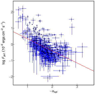
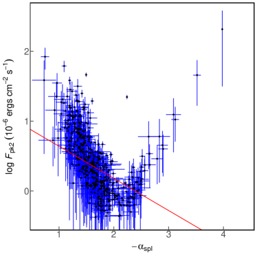
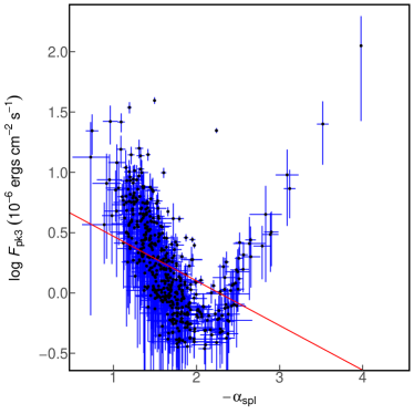
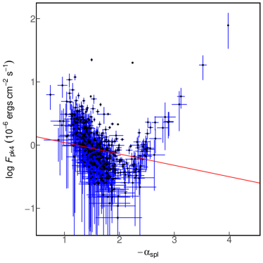
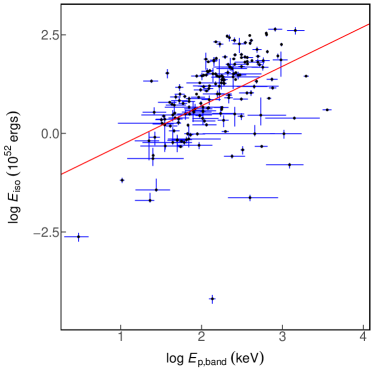
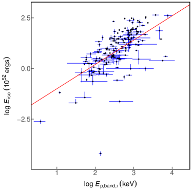
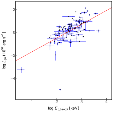
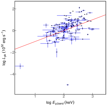
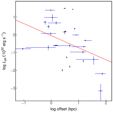
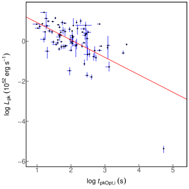
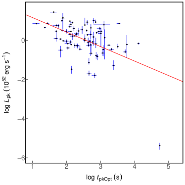
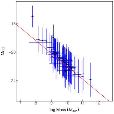
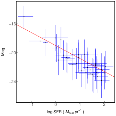
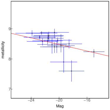
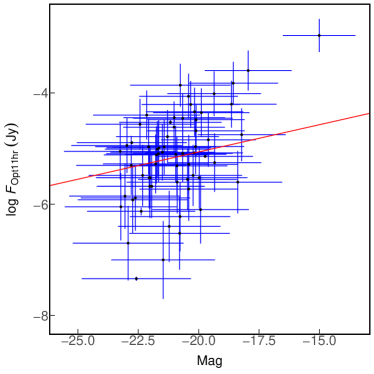
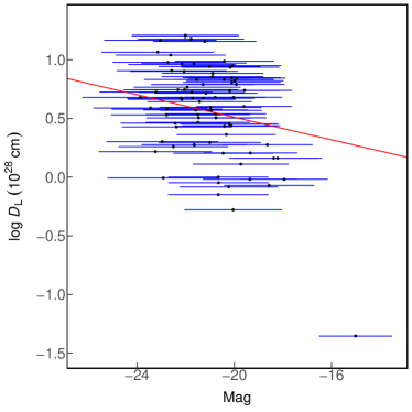
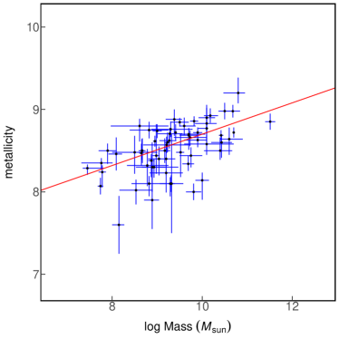
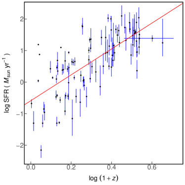
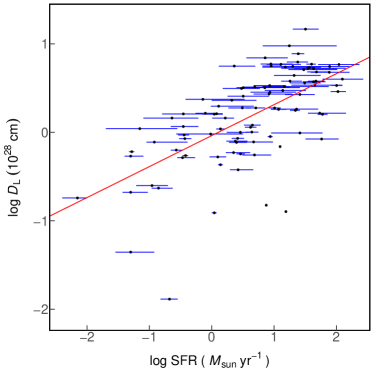
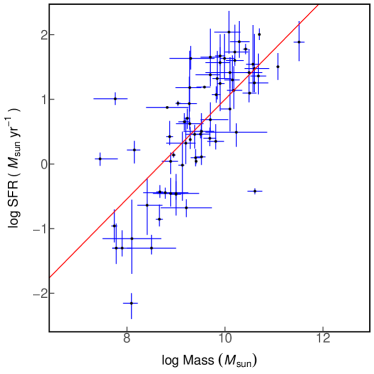
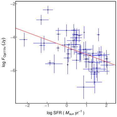
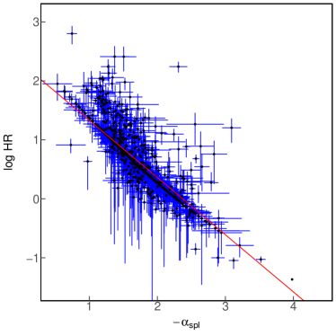
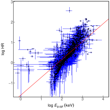
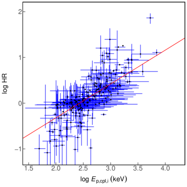
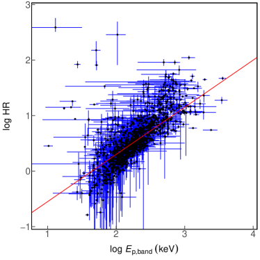
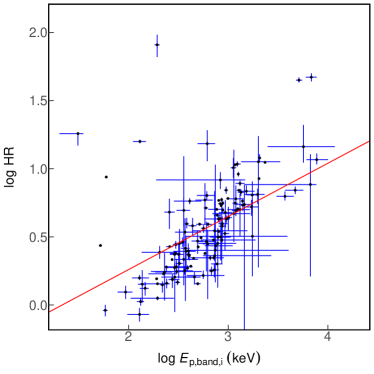
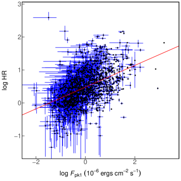
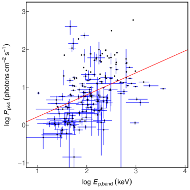
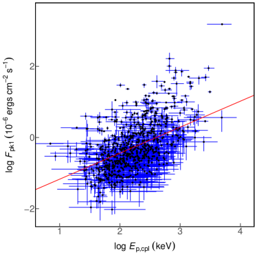
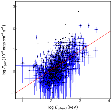
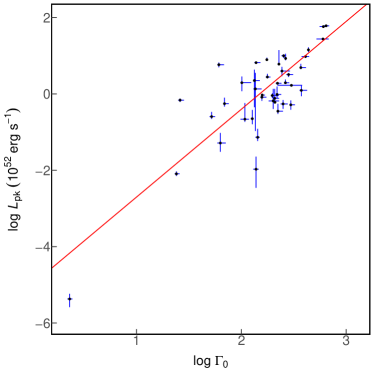
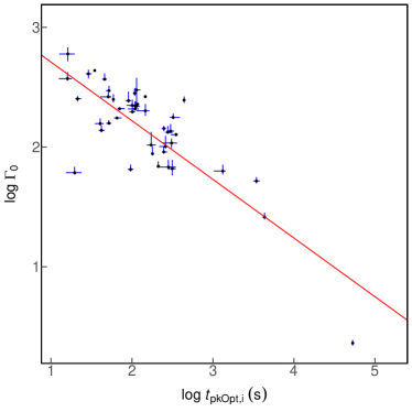
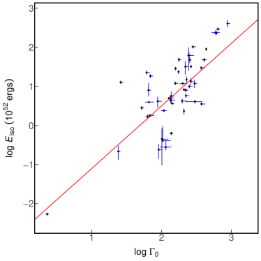
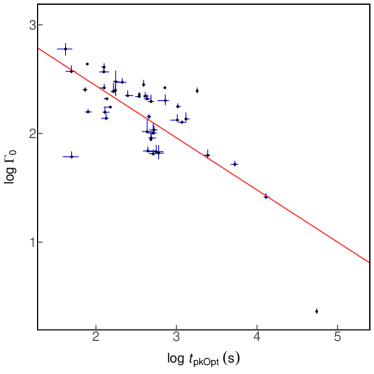
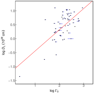
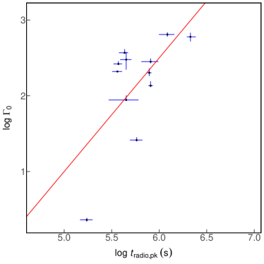
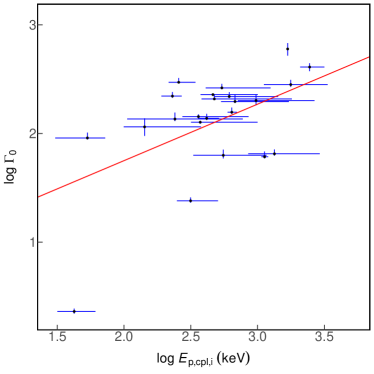
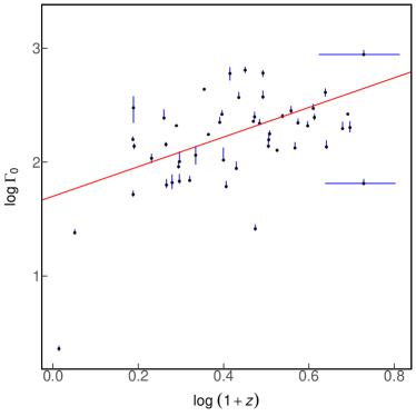
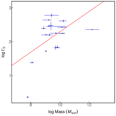
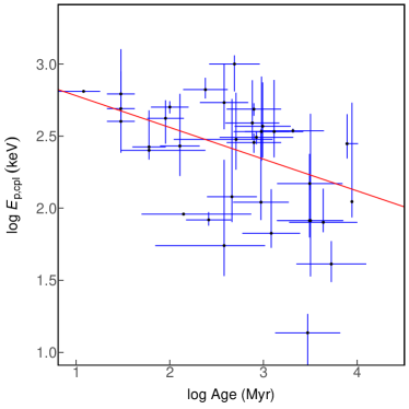
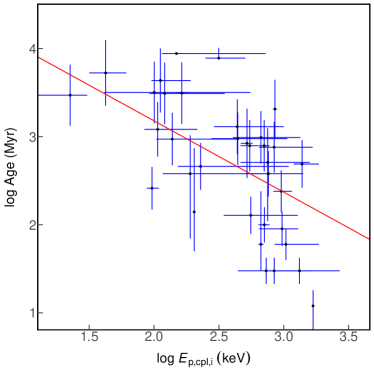
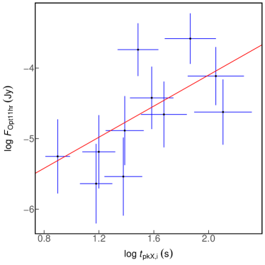
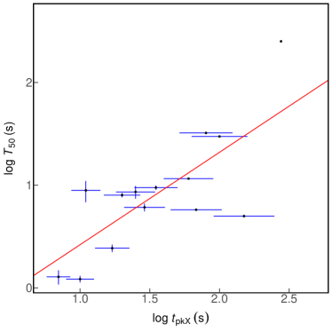
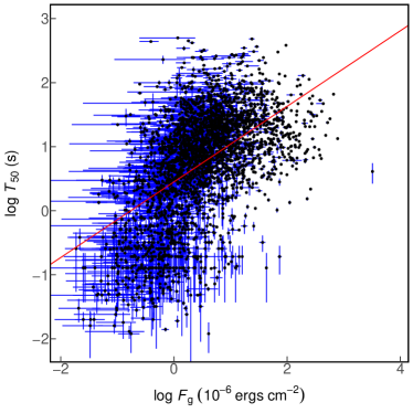
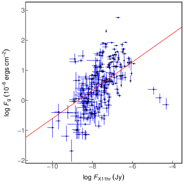
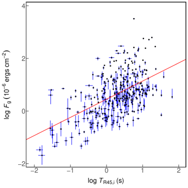
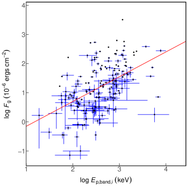
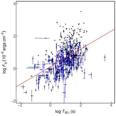
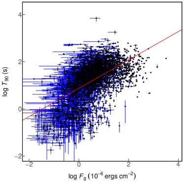
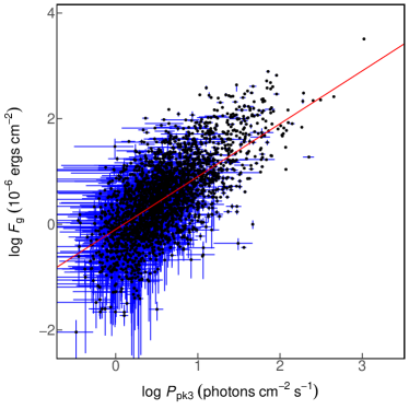
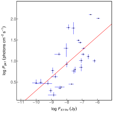
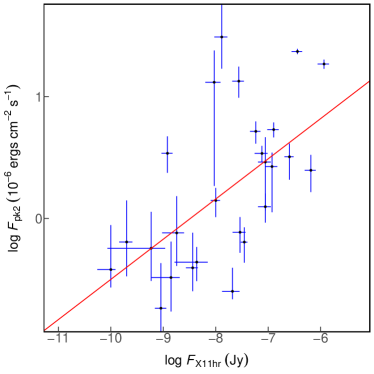
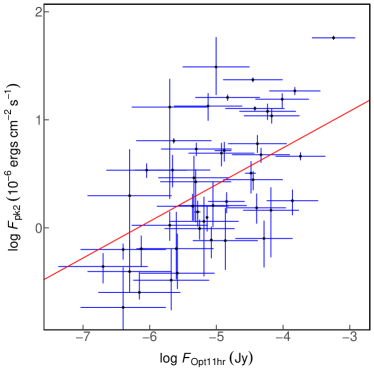
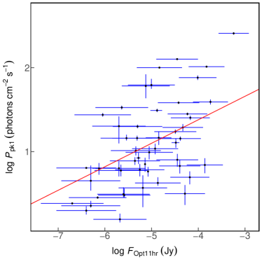
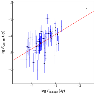
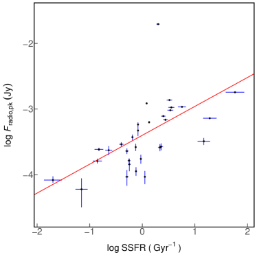
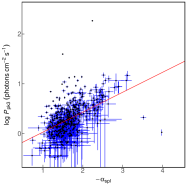
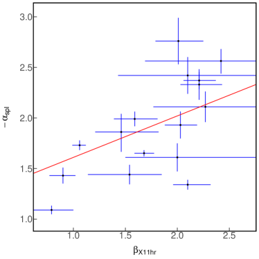
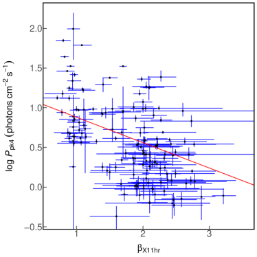
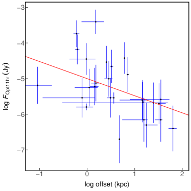
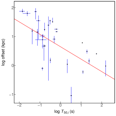
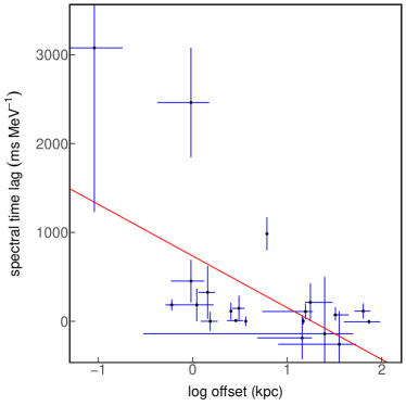
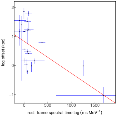
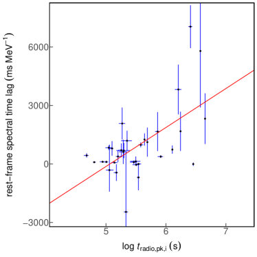
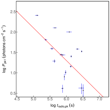
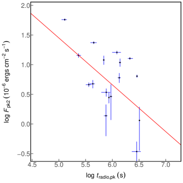
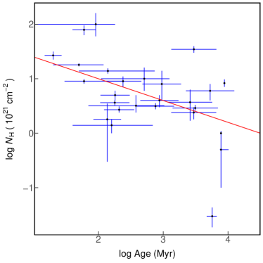
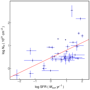
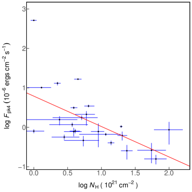
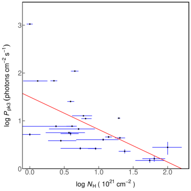
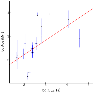
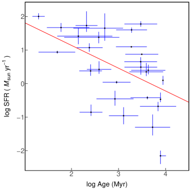
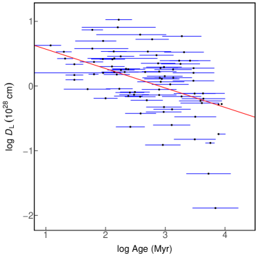
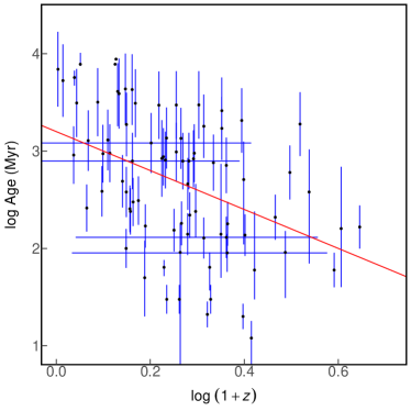
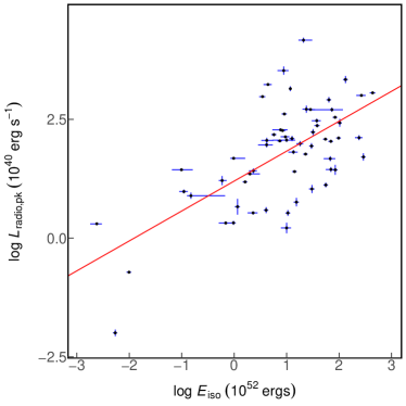
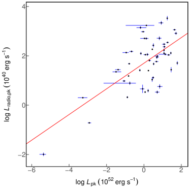
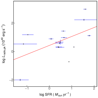
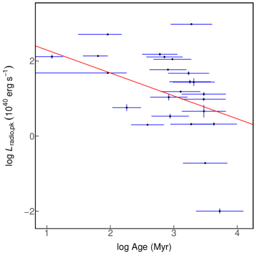
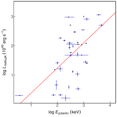
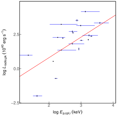
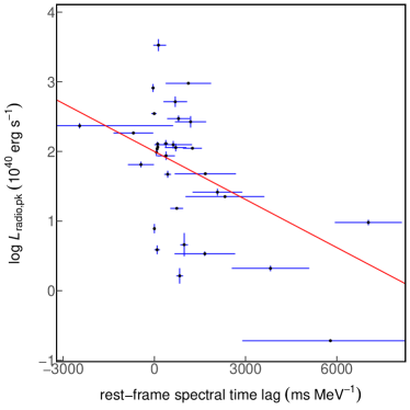
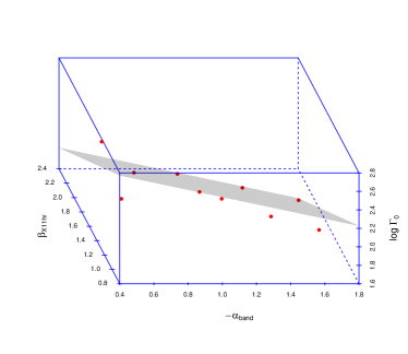
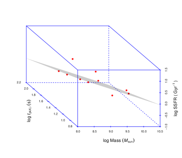
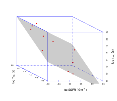
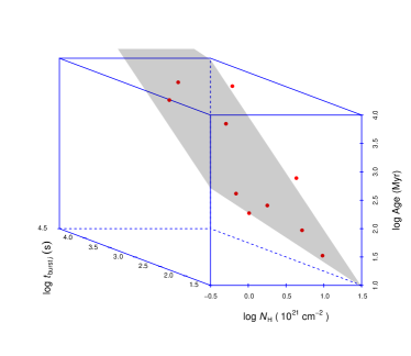
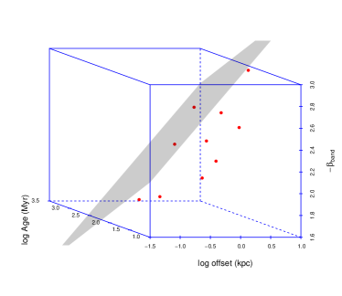
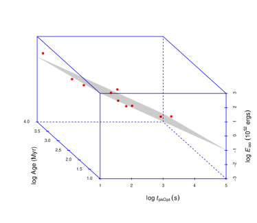
GRB	160509A	160422A	160419A	160417A	160412A
trigger time	08:59:04.36	11:59:00.81	15:16:37	04:23:41	04:23:54
instrument	Fermi/MAXI	Fermi/CGBM	Fermi/Swift	Swift	Swift
trigger number	484477130 160509374	483019143 160422499	482771799 160419637 683383	683076	682522
coordinate	$20h40m24s$ $+76\arcdeg 00\arcmin$	$02h48m12s$ $-57\arcdeg 54\arcmin$	$01h05m42s$ $-27\arcdeg 21\arcmin$	$08h00m58s$ $+07\arcdeg 38\arcmin$	$02h12m26s$ $-67\arcdeg 39\arcmin$
error	30	3	3	3	3
$z$	1.17	…	…	…	…
reference	(1)
$D_{\rm L}$ ($\rm 10^{\rm 28}~{}cm$)	2.27	…	…	…	…
reference
$T_{\rm 90}$ ($\rm s$)	$369.7^{\rm+0.8}_{\rm-0.8}$	$8.7^{\rm+0.18}_{\rm-0.18}$	$8.8^{\rm+0.67}_{\rm-0.67}$	$15^{\rm+1.2}_{\rm-1.2}$	$31.6^{\rm+2.4}_{\rm-2.4}$
reference	(1)	(3)	(5)	(7)	(8)
$T_{\rm 50}$ ($\rm s$)	…	…	…	…	…
reference
$T_{\rm R45}$ ($\rm s$)	…	…	…	…	…
reference
$variability_{\rm 1}$	…	…	…	…	…
reference
$variability_{\rm 2}$	…	…	…	…	…
reference
$variability_{\rm 3}$	…	…	…	…	…
reference
$F_{\rm g}$ ($\rm 10^{\rm-6}~{}ergs~{}cm^{\rm-2}$)	$218.1^{\rm+1.8}_{\rm-1.8}$	$95.15^{\rm+1.26}_{\rm-1.26}$	$4.6^{\rm+0.73}_{\rm-0.73}$	$1.3^{\rm+0.4}_{\rm-0.4}$	$4.56^{\rm+0.5}_{\rm-0.5}$
reference	(1)	(4)	(6)	(6)	(6)
HR	$5.853^{\rm+0.056}_{\rm-0.056}$	$3.383^{\rm+0.011}_{\rm-0.011}$	$0.88^{\rm+0.23}_{\rm-0.23}$	$2.19^{\rm+0.7}_{\rm-0.7}$	$2.46^{\rm+0.26}_{\rm-0.26}$
reference
$E_{\rm\gamma,iso}$ ($\rm 10^{\rm 52}~{}ergs$)	$57.6^{\rm+0.5}_{\rm-0.5}$	…	…	…	…
reference	(1)
$L_{\rm pk}$ ($\rm 10^{\rm 52}~{}ergs~{}s^{\rm-1}$)	…	…	…	…	…
reference
$F_{\rm pk1}$ ($\rm 10^{\rm-6}~{}ergs~{}cm^{\rm-2}~{}s^{\rm-1}$)	$21.86^{\rm+0.89}_{\rm-0.89}$	$19.29^{\rm+0.89}_{\rm-0.89}$	$1.06^{\rm+0.19}_{\rm-0.19}$	$0.27^{\rm+0.11}_{\rm-0.11}$	$0.474^{\rm+0.08}_{\rm-0.08}$
reference
$F_{\rm pk2}$ ($\rm 10^{\rm-6}~{}ergs~{}cm^{\rm-2}~{}s^{\rm-1}$)	…	…	…	…	…
$F_{\rm pk3}$ ($\rm 10^{\rm-6}~{}ergs~{}cm^{\rm-2}~{}s^{\rm-1}$)	…	…	…	…	…
$F_{\rm pk4}$ ($\rm 10^{\rm-6}~{}ergs~{}cm^{\rm-2}~{}s^{\rm-1}$)	…	…	…	…	…
$P_{\rm pk1}$ ($\rm photons~{}cm^{\rm-2}~{}s^{\rm-1}$)	…	…	…	…	…
reference
$P_{\rm pk2}$ ($\rm photons~{}cm^{\rm-2}~{}s^{\rm-1}$)	…	…	…	…	…
reference
$P_{\rm pk3}$ ($\rm photons~{}cm^{\rm-2}~{}s^{\rm-1}$)	…	…	…	…	…
reference
$P_{\rm pk4}$ ($\rm photons~{}cm^{\rm-2}~{}s^{\rm-1}$)	$71.27^{\rm+0.66}_{\rm-0.66}$	$93.8^{\rm+0.6}_{\rm-0.6}$	$11.51^{\rm+0.99}_{\rm-0.99}$	$1.63^{\rm+0.33}_{\rm-0.33}$	$2.59^{\rm+0.21}_{\rm-0.21}$
reference	(2)	(4)	(6)	(6)	(6)
$-\alpha_{\rm band}$	$0.89^{\rm+0.01}_{\rm-0.01}$	$0.95^{\rm+0.01}_{\rm-0.01}$	…	…	…
reference	(2)	(4)
$-\beta_{\rm band}$	$2.11^{\rm+0.02}_{\rm-0.02}$	$2.42^{\rm+0.04}_{\rm-0.04}$	…	…	…
reference	(2)	(4)
$E_{\rm p,band}$ ($\rm keV$)	$370^{\rm+7}_{\rm-7}$	$242^{\rm+4}_{\rm-4}$	…	…	…
reference	(2)	(4)
$-\alpha_{\rm cpl}$	…	…	$0.76^{\rm+0.2}_{\rm-0.2}$	…	…
reference			(5)
$E_{\rm p,cpl}$ ($\rm keV$)	…	…	$107.1^{\rm+21.29}_{\rm-21.29}$	…	…
reference			(5)
$-\alpha_{\rm spl}$	…	…	…	$1.93^{\rm+0.15}_{\rm-0.15}$	$1.88^{\rm+0.048}_{\rm-0.048}$
reference				(7)	(8)
$\theta_{\rm j}$ ($\rm rad$)	…	…	…	…	…
reference
spectral time lag ($\rm ms~{}MeV^{\rm-1}$)	…	…	…	…	…
reference
$\Gamma_{0}$	…	…	…	…	…
reference
$\log t_{\rm burst}$ ($\rm s$)	…	…	…	…	…
reference
$t_{\rm pkX}$ ($\rm s$)	…	…	…	…	…
reference
$t_{\rm pkOpt}$ ($\rm s$)	…	…	…	…	…
reference
$F_{\rm X11hr}$ ($\rm 10^{\rm-23}~{}ergs~{}cm^{\rm-2}~{}s^{\rm-1}~{}Hz^{\rm-1}$)	…	…	…	…	…
reference
$\beta_{\rm X11hr}$	…	…	…	…	…
reference
$F_{\rm Opt11hr}$ ($\rm 10^{\rm-23}~{}ergs~{}cm^{\rm-2}~{}s^{\rm-1}~{}Hz^{\rm-1}$)	…	…	…	…	…
reference
$t_{\rm radio,pk}$ ($\rm s$)	…	…	…	…	…
reference
$F_{\rm radio,pk}$ ($\rm 10^{\rm-23}~{}ergs~{}cm^{\rm-2}~{}s^{\rm-1}~{}Hz^{\rm-1}$)	…	…	…	…	…
reference
host galaxy offset ($\rm kpc$)	…	…	…	…	…
reference
metallicity	…	…	…	…	…
reference
Mag	…	…	…	…	…
reference
$N_{\rm H}$ ($\rm 10^{\rm 21}~{}cm^{\rm-2}$)	…	…	…	…	…
reference
$A_{\rm V}$	…	…	…	…	…
reference
SFR ($\rm M_{\bigodot}~{}yr^{\rm-1}$)	…	…	…	…	…
reference
$\log SSFR$ ($\rm Gyr^{\rm-1}$)	…	…	…	…	…
reference
Age ($\rm Myr$)	…	…	…	…	…
reference
$\log Mass$ ($M_{\bigodot}$)	…	…	…	…	…
reference

Note. — All the results are in machine readable table. The description of every parameter is in Section 2.

References. (1) Laskar et al. (2016); (2) Roberts et al. (2016); (3) Ricciarini et al. (2016); (4) Burns & Meegan (2016); (5) Cummings et al. (2016a); (6) https://swift.gsfc.nasa.gov/archive/grb_table/index.php; (7) Barthelmy et al. (2016a); (8) Ukwatta et al. (2016a); (9) Stamatikos et al. (2016a); (10) Sakamoto et al. (2016a); (11) Frederiks et al. (2016); (12) Palmer et al. (2016a); (13) Roberts (2016); (14) Mereghetti et al. (2016); (15) Markwardt et al. (2016a); (16) Lien et al. (2016b); (17) Krimm et al. (2016a); (18) Hui (2016); (19) Cummings et al. (2016b); (20) Barthelmy et al. (2016b); (21) Toelge & Hui (2016); (22) Ukwatta et al. (2016b); (23) Stamatikos et al. (2016b); (24) Sakamoto et al. (2016b); (25) Palmer et al. (2016b); (26) Ozawa et al. (2016); (27) von Kienlin et al. (2016); (28) Markwardt et al. (2016b); (29) Hui & Bissaldi (2016); (30) Lien et al. (2016c); (31) Krimm et al. (2016b); (32) Barthelmy et al. (2016c); (33) Barthelmy et al. (2016d); (34) Dado & Dar (2016); (35) Cummings et al. (2016c); (36) Barthelmy et al. (2016e); (37) Barthelmy et al. (2016f); (38) Ukwatta et al. (2016c); (39) Stamatikos et al. (2016c); (40) Palmer et al. (2016c); (41) Roberts & Burns (2016); (42) Nakahira et al. (2016); (43) Veres & Meegan (2016); (44) Palmer et al. (2016d); (45) Golenetskii et al. (2016a); (46) Yamada et al. (2016); (47) Veres (2016); (48) Moriyama et al. (2016); (49) Veres et al. (2015b); (50) Lien et al. (2015a); (51) Krimm et al. (2015a); (52) Barthelmy et al. (2015a); (53) Bissaldi et al. (2015b); (54) Senuma et al. (2015); (55) Toelge & Bissaldi (2015); (56) Kawakubo et al. (2015); (57) Golenetskii et al. (2016b); (58) Yu (2015a); (59) Cummings et al. (2015a); (60) Barthelmy et al. (2015b); (61) Ukwatta et al. (2015a); (62) Stamatikos et al. (2015a); (63) Sakamoto et al. (2015a); (64) Stanbro (2015a); (65) von Kienlin (2015a); (66) Markwardt et al. (2015a); (67) Lien et al. (2015b); (68) Krimm et al. (2015b); (69) Cummings et al. (2015i); (70) Yoshida et al. (2015); (71) Stanbro & Meegan (2015); (72) Malesani et al. (2015); (73) Ukwatta et al. (2015b); (74) Tanvir et al. (2015a); (75) Stamatikos et al. (2015b); (76) Xu et al. (2015); (77) Sakamoto et al. (2015b); (78) Nappo et al. (2017); (79) Palmer et al. (2015a); (80) Markwardt et al. (2015b); (81) Lien et al. (2015c); (82) Krimm et al. (2015c); (83) Cummings et al. (2015b); (84) Barthelmy et al. (2015c); (85) Ukwatta et al. (2015c); (86) Stamatikos et al. (2015c); (87) Sakamoto et al. (2015c); (88) Roberts et al. (2015a); (89) Golenetskii et al. (2015b); (90) Augusto et al. (2016); (91) Palmer et al. (2015b); (92) Bissaldi (2015); (93) Markwardt et al. (2015c); (94) Zheng et al. (2009); (95) Lien et al. (2015d); (96) Krimm et al. (2015d); (97) Golenetskii et al. (2015c); (98) Roberts & Younes (2015a); (99) Cummings et al. (2015c); (100) Barthelmy et al. (2015d); (101) Ukwatta et al. (2015d); (102) Bissaldi & Burns (2015); (103) D’Elia et al. (2015); (104) Stamatikos et al. (2015d); (105) Roberts (2015a); (106) Yu & Burns (2015); (107) Sakamoto et al. (2015d); (108) Cano et al. (2017); (109) Palmer et al. (2015c); (110) Markwardt et al. (2015d); (111) Yu & Jenke (2015); (112) Jenke (2015a); (113) Krimm et al. (2015e); (114) Barthelmy et al. (2015e); (115) Ukwatta et al. (2015e); (116) Tanvir et al. (2015b); (117) Stamatikos et al. (2015e); (118) Younes (2015); (119) Golenetskii et al. (2015d); (120) Veres et al. (2015a); (121) Palmer et al. (2015d); (122) Markwardt et al. (2015e); (123) Bissaldi et al. (2015a); (124) Lien et al. (2015e); (125) Lien et al. (2015f); (126) Krimm et al. (2015f); (127) Jenke (2015b); (128) Cummings et al. (2015d); (129) Barthelmy et al. (2015f); (130) Jenke (2015c); (131) Yu et al. (2015b); (132) Ukwatta et al. (2015f); (133) Stamatikos et al. (2015f); (134) Sakamoto et al. (2015e); (135) Golenetskii et al. (2015e); (136) Palmer et al. (2015e); (137) Roberts (2015b); (138) Cummings & Palmer (2015); (139) Markwardt et al. (2015f); (140) Yu et al. (2015c); (141) Lien et al. (2015g); (142) Yu (2015b); (143) Fujinuma et al. (2015); (144) de Ugarte Postigo et al. (2015); (145) Roberts et al. (2015b); (146) Lien et al. (2015h); (147) Younes & Meegan (2015); (148) Burns & Meegan (2015a); (149) Krimm et al. (2015g); (150) Roberts & Younes (2015b); (151) Zhang et al. (2014a); (152) Cummings et al. (2015e); (153) Baumgartner et al. (2015a); (154) Barthelmy et al. (2015g); (155) Siellez et al. (2016); (156) Ukwatta et al. (2015g); (157) Golenetskii et al. (2015f); (158) Deng et al. (2016); (159) Stamatikos et al. (2015g); (160) Sakamoto et al. (2015f); (161) Dichiara et al. (2016); (162) Zhang (2015); (163) Stanbro (2015b); (164) Palmer et al. (2015f); (165) von Kienlin (2015b); (166) Markwardt et al. (2015g); (167) Lien et al. (2015i); (168) Krimm et al. (2015h); (169) Cummings et al. (2015f); (170) Yu (2015c); (171) Baumgartner et al. (2015b); (172) Roberts & Stanbro (2015); (173) Barthelmy et al. (2015h); (174) Stamatikos et al. (2015h); (175) Gorbovskoy et al. (2016); (176) Burns & Meegan (2015b); (177) Sakamoto et al. (2015g); (178) Connaughton et al. (2015); (179) Markwardt et al. (2015h); (180) von Kienlin & Meegan (2015); (181) Mereghetti et al. (2015); (182) Krimm et al. (2015i); (183) Cummings et al. (2015g); (184) Baumgartner et al. (2015c); (185) Burns (2015a); (186) Barthelmy et al. (2015i); (187) Stamatikos et al. (2015i); (188) Burns & Yu (2015); (189) Ukwatta et al. (2015h); (190) Pelassa & Yu (2015); (191) Pelassa (2015); (192) Sakamoto et al. (2015h); (193) Palmer et al. (2015g); (194) Jenke & von Kienlin (2015); (195) Stanbro (2015c); (196) Golenetskii et al. (2015a); (197) Wiseman et al. (2015); (198) Markwardt et al. (2015i); (199) Sang et al. (2016); (200) Lien et al. (2015j); (201) von Kienlin & Burns (2015); (202) Burns (2015b); (203) Stanbro (2015d); (204) Stanbro (2015e); (205) Stanbro & Yu (2015); (206) Cummings et al. (2015h); (207) Xie et al. (2016); (208) Fong et al. (2015); (209) Stanbro (2015f); (210) Baumgartner et al. (2015d); (211) Cummings et al. (2014a); (212) Roberts (2014d); (213) Barthelmy et al. (2014a); (214) Jenke (2014a); (215) Jenke (2014b); (216) Ukwatta et al. (2014a); (217) Yu (2014a); (218) Ghirlanda et al. (2017); (219) Lin et al. (2016); (220) Stamatikos et al. (2014a); (221) Jenke et al. (2014); (222) Sakamoto et al. (2014a); (223) Palmer et al. (2014a); (224) Liu et al. (2015); (225) Burns (2014a); (226) Markwardt et al. (2014a); (227) Roberts (2014e); (228) Roberts (2014f); (229) Lien et al. (2014a); (230) Krimm et al. (2014a); (231) Cucchiara et al. (2015); (232) Jenke (2014c); (233) Cummings et al. (2014b); (234) Baumgartner et al. (2014a); (235) Cummings (2014a); (236) Zhang (2014a); (237) Barthelmy et al. (2014b); (238) Ukwatta et al. (2014b); (239) Roberts (2014g); (240) Roberts (2014h); (241) Xu et al. (2014); (242) Roberts (2014c); (243) Ruffini et al. (2016); (244) Stamatikos et al. (2014b); (245) Sakamoto et al. (2014b); (246) Palmer et al. (2014b); (247) Markwardt et al. (2014b); (248) Turpin et al. (2016); (249) Lien et al. (2014b); (250) von Kienlin (2014a); (251) Krimm et al. (2014b); (252) Roberts (2014a); (253) Cummings et al. (2014c); (254) Pelassa (2014a); (255) Baumgartner et al. (2014b); (256) von Kienlin & Meegan (2014); (257) Barthelmy et al. (2014c); (258) Ukwatta et al. (2014c); (259) Pelassa (2014b); (260) Stamatikos et al. (2014c); (261) Sakamoto et al. (2014c); (262) Zhang (2014b); (263) Golenetskii et al. (2014a); (264) Palmer et al. (2014c); (265) Troja et al. (2016); (266) Zhang (2014c); (267) Jenke (2014d); (268) Markwardt et al. (2014c); (269) von Kienlin (2014b); (270) Golenetskii et al. (2014b); (271) Lien et al. (2014c); (272) Krimm et al. (2014c); (273) Roberts (2014b); (274) Cummings et al. (2014d); (275) Roberts & Meegan (2014); (276) Roberts & Stanbro (2014); (277) Zhang (2014d); (278) Lipunov et al. (2016); (279) Pelassa (2014c); (280) Baumgartner et al. (2014c); (281) Stanbro (2014a); (282) Burns (2014b); (283) Barthelmy et al. (2014d); (284) Ukwatta et al. (2014d); (285) Cummings et al. (2014e); (286) Jenke & Yu (2014); (287) Stamatikos et al. (2014d); (288) Zhang (2014e); (289) Narayana Bhat et al. (2016); (290) Burns (2014c); (291) Sakamoto et al. (2014d); (292) Littlejohns et al. (2015); (293) Zhang (2014f); (294) Zhang (2014g); (295) Pescalli et al. (2016); (296) Cummings et al. (2014f); (297) Stamatikos et al. (2014e); (298) Younes et al. (2014b); (299) von Kienlin (2014c); (300) Younes & Meegan (2014); (301) Connaughton et al. (2014); (302) Palmer et al. (2014d); (303) Barthelmy et al. (2014e); (304) Markwardt et al. (2014d); (305) Golenetskii et al. (2014c); (306) Stanbro (2014b); (307) Krimm et al. (2014d); (308) Li et al. (2016); (309) Cano et al. (2015); (310) Cummings et al. (2014g); (311) Golenetskii et al. (2014d); (312) Cummings et al. (2014h); (313) Stanbro (2014c); (314) Golenetskii et al. (2014e); (315) Stanbro & Troja (2014); (316) Ukwatta et al. (2014e); (317) Stamatikos et al. (2014f); (318) Stamatikos et al. (2014g); (319) Melandri et al. (2015); (320) Palmer et al. (2014e); (321) Krühler et al. (2015); (322) Yu (2014b); (323) Yu (2014c); (324) Kopač et al. (2015); (325) Younes (2014a); (326) Krimm et al. (2014e); (327) Jenke (2014e); (328) Cummings (2014b); (329) Barthelmy et al. (2014f); (330) Ukwatta et al. (2014f); (331) Jenke & Fitzpatrick (2014); (332) Yu (2014d); (333) Cummings (2014c); (334) Stamatikos et al. (2014h); (335) Pelassa et al. (2014); (336) von Kienlin & Younes (2014); (337) Yu & von Kienlin (2014); (338) Golenetskii et al. (2014f); (339) Younes et al. (2014a); (340) Markwardt et al. (2014e); (341) Stanbro (2014d); (342) Stanbro (2014e); (343) Krimm et al. (2014f); (344) Golenetskii et al. (2014g); (345) Fitzpatrick & Stanbro (2014); (346) Cummings et al. (2014i); (347) Barthelmy et al. (2014g); (348) Ukwatta et al. (2014g); (349) Zhang (2014h); (350) Barthelmy et al. (2014h); (351) Stamatikos et al. (2014i); (352) Cummings et al. (2014j); (353) von Kienlin (2014d); (354) von Kienlin (2014e); (355) Palmer et al. (2014f); (356) Markwardt et al. (2014f); (357) Xiong (2014a); (358) Krimm et al. (2014g); (359) Greiner et al. (2015); (360) von Kienlin & Connaughton (2014); (361) Younes (2014b); (362) Xiong et al. (2014); (363) Xiong (2014b); (364) Baumgartner et al. (2014e); (365) von Kienlin & Bhat (2014); (366) Racusin et al. (2016); (367) Barthelmy et al. (2013a); (368) Stamatikos et al. (2013a); (369) Pelassa (2013a); (370) Golenetskii et al. (2014h); (371) von Kienlin & Meegan (2013a); (372) Sakamoto et al. (2013a); (373) Collazzi (2013a); (374) Yu (2013a); (375) von Kienlin (2013a); (376) Markwardt et al. (2013a); (377) Pelassa & Meegan (2013); (378) Golenetskii et al. (2013a); (379) Lien et al. (2013a); (380) Collazzi (2013b); (381) Krimm et al. (2013a); (382) Barthelmy et al. (2013b); (383) Fitzpatrick & Bhat (2013); (384) Barthelmy et al. (2013c); (385) Urata et al. (2015); (386) von Kienlin & Jenke (2013); (387) von Kienlin (2013b); (388) Zhang (2013a); (389) Barthelmy et al. (2013d); (390) Zhang (2013b); (391) Ukwatta et al. (2013a); (392) Fitzpatrick & Xiong (2013); (393) Jenke (2013a); (394) Xiong (2013a); (395) Golkhou & Butler (2014); (396) Sato et al. (2013); (397) von Kienlin & Meegan (2013b); (398) Cummings et al. (2013); (399) Palmer et al. (2013a); (400) Greiner et al. (2014); (401) Lien et al. (2013b); (402) Zhang et al. (2013a); (403) Xiong & Meegan (2013); (404) Baumgartner et al. (2013); (405) Cano et al. (2014); (406) Zhang et al. (2016a); (407) Beskin et al. (2015); (408) Collazzi (2013c); (409) Ukwatta et al. (2013b); (410) Golenetskii et al. (2013b); (411) Stamatikos et al. (2013b); (412) Fitzpatrick & Younes (2013); (413) Golenetskii et al. (2013c); (414) Palmer et al. (2013b); (415) Markwardt et al. (2013b); (416) Lien et al. (2013c); (417) Yu et al. (2013); (418) Goldstein (2013a); (419) Barthelmy et al. (2013e); (420) Ukwatta et al. (2013c); (421) Golenetskii et al. (2013d); (422) Stamatikos et al. (2013c); (423) Foley & Meegan (2013); (424) Collazzi (2013d); (425) Fitzpatrick (2013); (426) Wang & Dai (2014); (427) Pelassa (2013b); (428) Contopoulos et al. (2014); (429) Stamatikos et al. (2013d); (430) Byrne (2013); (431) Sakamoto et al. (2013b); (432) Palmer et al. (2013c); (433) Byrne et al. (2013); (434) Barthelmy et al. (2013f); (435) Xiong (2013b); (436) Wang et al. (2016); (437) Golenetskii et al. (2013e); (438) Fitzpatrick & Burgess (2013); (439) Krimm et al. (2013b); (440) Yu et al. (2015d); (441) Yu (2013b); (442) Yu et al. (2015a); (443) Golenetskii et al. (2013f); (444) Collazzi (2013e); (445) Berger (2014); (446) Barthelmy et al. (2013g); (447) Krimm et al. (2013c); (448) Jeong et al. (2014); (449) Golenetskii et al. (2013g); (450) Barthelmy et al. (2013h); (451) Krimm & Cummings (2013); (452) Jenke (2013b); (453) Cummings & Krimm (2013); (454) Ukwatta et al. (2013d); (455) Sakamoto et al. (2013c); (456) Burgess et al. (2013); (457) von Kienlin (2013c); (458) Palmer et al. (2013d); (459) von Kienlin & Younes (2013); (460) Goldstein et al. (2016); (461) Song et al. (2016); (462) Gao et al. (2015b); (463) Japelj et al. (2014); (464) Niino et al. (2016); (465) von Kienlin (2013d); (466) Rau (2013); (467) Zhang et al. (2015a); (468) Krimm et al. (2013d); (469) Wei et al. (2014); (470) Serino et al. (2014); (471) Chaplin & Fitzpatrick (2013); (472) Barthelmy et al. (2013i); (473) Tierney (2013); (474) Golenetskii et al. (2013h); (475) Barthelmy et al. (2013j); (476) Barthelmy et al. (2013k); (477) D’Avanzo et al. (2014); (478) Norris et al. (2013); (479) Xiong & Chaplin (2013); (480) Pelassa (2013c); (481) Golenetskii et al. (2013i); (482) Yu & Xiong (2013); (483) Chaplin (2013a); (484) Chaplin (2013b); (485) Ukwatta et al. (2013e); (486) Goldstein (2013b); (487) Palmer et al. (2013e); (488) Pelassa (2013d); (489) Barthelmy et al. (2013l); (490) Golenetskii et al. (2013j); (491) Markwardt et al. (2013c); (492) Lü & Zhang (2014); (493) Baumgartner et al. (2012e); (494) Golenetskii et al. (2012v); (495) Liang et al. (2015); (496) Baumgartner et al. (2012e); (497) Heussaff et al. (2013); (498) Tierney (2012); (499) Golenetskii et al. (2012w); (500) Golenetskii et al. (2012x); (501) Golenetskii et al. (2012y); (502) Baumgartner et al. (2012f); (503) Baumgartner et al. (2012g); (504) Goldstein & Meegan (2012); (505) Kaneko et al. (2015); (506) Sakamoto et al. (2012b); (507) Ukwatta et al. (2012c); (508) Barthelmy et al. (2012n); (509) Pelassa (2012b); (510) Xiong et al. (2012); (511) Sakamoto et al. (2012e); (512) Palmer et al. (2012e); (513) Markwardt et al. (2012c); (514) Golenetskii et al. (2012z); (515) Golenetskii  et al. (2012c); (516) Barthelmy et al. (2012f); (517) Golenetskii  et al. (2012a); (518) Pelassa (2012c); (519) Pelassa & Connaughton (2012); (520) Golenetskii  et al. (2012b); (521) Gruber (2012b); (522) McGlynn (2012); (523) Golenetskii et al. (2012r); (524) Sakamoto et al. (2012c); (525) Golenetskii et al. (2012s); (526) Palmer et al. (2012d); (527) Xu et al. (2013); (528) Golenetskii et al. (2012u); (529) Barthelmy et al. (2012g); (530) Golenetskii et al. (2012t); (531) Barthelmy et al. (2012h); (532) Cummings et al. (2012a); (533) Barthelmy et al. (2012i); (534) Baumgartner et al. (2012d); (535) Barthelmy et al. (2012d); (536) Ukwatta et al. (2012d); (537) Golenetskii et al. (2012q); (538) Markwardt et al. (2012d); (539) Dereli et al. (2015); (540) Cummings et al. (2012b); (541) Baumgartner et al. (2012c); (542) von Kienlin et al. (2014); (543) Ukwatta et al. (2012e); (544) Golenetskii et al. (2012p); (545) Golenetskii et al. (2012o); (546) Barthelmy et al. (2012j); (547) Sakamoto et al. (2012a); (548) Golenetskii et al. (2012n); (549) Palmer et al. (2012c); (550) Golenetskii et al. (2012m); (551) Golenetskii et al. (2012l); (552) Golenetskii et al. (2012k); (553) Markwardt et al. (2012b); (554) Gruber (2012a); (555) Cummings et al. (2012c); (556) Golenetskii et al. (2012j); (557) Baumgartner et al. (2012b); (558) Golenetskii et al. (2012i); (559) Golenetskii et al. (2012h); (560) Golenetskii et al. (2012g); (561) Laskar et al. (2015); (562) Younes (2012); (563) Sakamoto et al. (2012d); (564) Collazzi (2012); (565) Palmer et al. (2012b); (566) Golenetskii et al. (2012f); (567) Markwardt et al. (2012a); (568) D’Elia et al. (2014); (569) Golenetskii et al. (2012e); (570) Golenetskii et al. (2012d); (571) Golenetskii et al. (2012c); (572) Barthelmy et al. (2012c); (573) Ukwatta et al. (2012b); (574) Stamatikos et al. (2012); (575) Palmer et al. (2012a); (576) Norris & Barthelmy (2012); (577) Pelassa (2012a); (578) Markwardt et al. (2012e); (579) Golenetskii et al. (2012b); (580) Barthelmy et al. (2012k); (581) Cummings et al. (2012d); (582) Barthelmy et al. (2012b); (583) Barthelmy et al. (2012l); (584) Baumgartner et al. (2012a); (585) Rau (2012); (586) Ukwatta et al. (2012f); (587) Bošnjak et al. (2014); (588) Barthelmy et al. (2012m); (589) Perley et al. (2016a); (590) Golenetskii et al. (2012a); (591) Barthelmy et al. (2012a); (592) Rau & Meegan (2012); (593) Golenetskii et al. (2011j); (594) Barthelmy et al. (2011f); (595) Wei et al. (2016); (596) Ukwatta et al. (2011d); (597) Stamatikos et al. (2011b); (598) Gao et al. (2016); (599) Kann et al. (2016); (600) Stratta et al. (2013); (601) Golenetskii et al. (2011i); (602) Markwardt et al. (2011a); (603) Barthelmy et al. (2011g); (604) Cummings et al. (2011b); (605) Margutti et al. (2012); (606) Baumgartner et al. (2011c); (607) Golenetskii et al. (2011h); (608) Tierney (2011); (609) Palmer et al. (2011c); (610) Barthelmy et al. (2011h); (611) Markwardt et al. (2011b); (612) Krimm et al. (2011b); (613) Sakamoto et al. (2011c); (614) Sakamoto et al. (2011a); (615) Cummings et al. (2011c); (616) Golenetskii et al. (2011g); (617) Barthelmy et al. (2011e); (618) Sparre et al. (2014); (619) Michałowski et al. (2015); (620) Greiner et al. (2016); (621) Barthelmy et al. (2011i); (622) Fitzpatrick (2011); (623) Frederiks et al. (2013); (624) Sakamoto et al. (2011d); (625) Golenetskii et al. (2011f); (626) Palmer et al. (2011b); (627) Golenetskii et al. (2011e); (628) Golenetskii et al. (2011d); (629) Tsutsui & Shigeyama (2013); (630) Ackermann et al. (2013); (631) Cummings et al. (2011d); (632) Baumgartner et al. (2011d); (633) Xiong (2011); (634) Baumgartner et al. (2011b); (635) Barthelmy et al. (2011j); (636) Ukwatta et al. (2011c); (637) Stamatikos et al. (2011a); (638) Golenetskii et al. (2011c); (639) Nava et al. (2012); (640) Melandri et al. (2012); (641) Allison et al. (2017); (642) Lin (2011); (643) Golenetskii et al. (2011b); (644) Cummings et al. (2011a); (645) Virgili et al. (2012); (646) Barthelmy et al. (2011d); (647) Ukwatta et al. (2011b); (648) Golenetskii et al. (2011a); (649) Palmer et al. (2011a); (650) Barthelmy et al. (2011c); (651) Markwardt et al. (2011c); (652) Krimm et al. (2011a); (653) Barthelmy et al. (2011k); (654) Cummings et al. (2011e); (655) Barthelmy et al. (2011b); (656) Baumgartner et al. (2011a); (657) Ukwatta et al. (2012a); (658) Ukwatta et al. (2011a); (659) Stamatikos et al. (2011c); (660) Sakamoto et al. (2011e); (661) von Kienlin (2011); (662) Cucchiara et al. (2011); (663) Chandra & Frail (2012); (664) Barthelmy et al. (2011a); (665) Cummings & Barthelmy (2011); (666) Stamatikos et al. (2011d); (667) Fermi Large Area Telescope Team et al. (2012); (668) Balázs et al. (2015); (669) Liu et al. (2016); (670) Kopač et al. (2012); (671) Tunnicliffe et al. (2014); (672) Foley (2010); (673) Frederiks (2010); (674) Baumgartner et al. (2010a); (675) Golenetskii et al. (2010c); (676) Barthelmy et al. (2010a); (677) Golenetskii et al. (2010b); (678) Gorbovskoy et al. (2012); (679) Sakamoto et al. (2010b); (680) Golenetskii et al. (2010a); (681) Krimm et al. (2010a); (682) Cummings et al. (2010b); (683) Baumgartner et al. (2010b); (684) Barthelmy et al. (2010b); (685) Ukwatta et al. (2010b); (686) Stamatikos et al. (2010a); (687) Sakamoto et al. (2010c); (688) Ghirlanda et al. (2012); (689) Barniol Duran (2014); (690) Geng et al. (2016); (691) Cummings et al. (2010a); (692) Barthelmy et al. (2010c); (693) von Kienlin (2010); (694) Sakamoto et al. (2010a); (695) Palmer et al. (2010a); (696) Ahlgren et al. (2015); (697) Markwardt et al. (2010); (698) Piranomonte et al. (2015); (699) Krimm et al. (2010b); (700) Barthelmy et al. (2010d); (701) Japelj et al. (2016); (702) Volnova et al. (2014); (703) Krühler et al. (2011); (704) Arcodia et al. (2016); (705) Cummings et al. (2010c); (706) Baumgartner et al. (2010c); (707) Afonso et al. (2010); (708) Stamatikos et al. (2010b); (709) Ripa (2011); (710) Cummings et al. (2010d); (711) Zhang et al. (2011); (712) Nava et al. (2011); (713) Levesque et al. (2010b); (714) Palmer et al. (2010b); (715) Greiner et al. (2011); (716) Baumgartner et al. (2010d); (717) Barthelmy et al. (2010e); (718) Sakamoto et al. (2010d); (719) Palmer et al. (2010c); (720) Yonetoku et al. (2010); (721) Sakamoto et al. (2011b); (722) Filgas et al. (2011); (723) Sakamoto et al. (2009); (724) Nemmen et al. (2012); (725) Lu et al. (2012b); (726) Wang et al. (2013); (727) Galli et al. (2013); (728) Robertson & Ellis (2012); (729) Guetta et al. (2011); (730) Butler et al. (2010); (731) Kopač et al. (2013); (732) Minaev et al. (2014); (733) Liang et al. (2009); (734) Qin & Chen (2013); (735) Zhang et al. (2009a); (736) Krimm et al. (2009); (737) Perley et al. (2013); (738) Lü et al. (2012); (739) Lien et al. (2016a); (740) Dichiara et al. (2013b); (741) Nardini et al. (2011); (742) Li et al. (2012b); (743) Golkhou et al. (2015); (744) Vianello et al. (2009); (745) Kann et al. (2010); (746) Huja et al. (2009); (747) Thoene et al. (2008); (748) Bhat et al. (2012); (749) Xiao & Schaefer (2011); (750) Schady et al. (2011); (751) Krühler et al. (2009); (752) Ukwatta et al. (2010a); (753) Řípa et al. (2009); (754) Nava et al. (2008); (755) Perley et al. (2009); (756) Nardini et al. (2010); (757) Zheng et al. (2009); (758) Cenko et al. (2009); (759) Minaev et al. (2010); (760) Rossi et al. (2008); (761) Hjorth et al. (2012); (762) Gehrels et al. (2008); (763) Nysewander et al. (2009); (764) Foley et al. (2008); (765) Xiao & Schaefer (2009b); (766) Graham & Fruchter (2013); (767) Kasliwal et al. (2008); (768) Schady et al. (2010); (769) Butler et al. (2007); (770) Perley et al. (2015); (771) Contini (2016); (772) Ghisellini et al. (2009); (773) Covino & Gotz (2016); (774) Gao & Dai (2010); (775) Savaglio et al. (2009); (776) Bellm et al. (2008); (777) Rizzuto et al. (2007); (778) Campisi & Li (2008); (779) Mosquera Cuesta et al. (2008); (780) Willingale et al. (2007b); (781) Schaefer (2007); (782) Rykoff et al. (2009); (783) Melandri et al. (2008); (784) Fong et al. (2010b); (785) De Laurentis et al. (2015); (786) Graham & Fruchter (2017); (787) Pélangeon et al. (2008); (788) Leibler & Berger (2010); (789) Collazzi & Schaefer (2008); (790) Xiao & Schaefer (2009a); (791) Levesque et al. (2010a); (792) Mannucci et al. (2011); (793) Tsutsui et al. (2013a); (794) Zaninoni et al. (2013); (795) Ghirlanda et al. (2007); (796) Guidorzi et al. (2016); (797) Tanvir et al. (2005); (798) Li et al. (2015); (799) Sakamoto et al. (2008); (800) Rau et al. (2005); (801) Guidorzi et al. (2005); (802) Friedman & Bloom (2005); (803) Sako et al. (2005); (804) Sakamoto et al. (2005); (805) Li et al. (2008); (806) Mazets et al. (2002); (807) Barraud et al. (2003); (808) Frontera (2004); (809) Frontera et al. (2009); (810) de Pasquale et al. (2006); (811) Guidorzi et al. (2011); (812) Atteia (2003); (813) Christensen et al. (2004); (814) https://gammaray.nsstc.nasa.gov/batse/grb/catalog/current/index.html; (815) Shahmoradi & Nemiroff (2010); (816) Goldstein et al. (2013); (817) Ashcraft & Schaefer (2007); (818) Ghirlanda et al. (2009); (819) Bloom et al. (2002); (820) Jimenez et al. (2001); (821) Kaneko et al. (2006); (822) Ramirez-Ruiz et al. (2002); (823) Smith et al. (2002); (824) Reichart et al. (2001); (825) Frail et al. (2001); (826) Schaefer (2003b); (827) Sokolov et al. (2001); (828) Simić & Č. Popović (2012); (829) Fenimore & Ramirez-Ruiz (2000); (830) Svensson et al. (2010); (831) Bosnjak et al. (2006); (832) Postnov (2000); (833) Bloom et al. (2001); (834) Berger et al. (2003); (835) Fragile et al. (2004); (836) Amati et al. (2008); (837) Wei (2010); (838) Paciesas et al. (1999); (839) Lloyd-Ronning & Ramirez-Ruiz (2002); (840) Peng et al. (2012); (841) Preece et al. (2000); (842) Meegan et al. (1996); (843) Sazonov et al. (1998); (844) Hakkila et al. (2007); (845) Fishman et al. (1994); (846) Terekhov et al. (1994)

Table 2: Imputation results

Parameters	RIV	FMI	RE	Parameters	RIV	FMI	RE
$T_{\rm 901}$	0.00000358	0.00000358	1	$T_{\rm 902}$	0.000126	0.000126	1
$T_{\rm 501}$	0.000143	0.000143	1	$T_{\rm 502}$	0.0000796	0.0000796	1
$T_{\rm R451}$	0.0122	0.0122	0.998	$T_{\rm R452}$	0.00172	0.00172	1
$variability_{\rm 11}$	0.0137	0.0136	0.997	$variability_{\rm 12}$	0.00491	0.0049	0.999
$F_{\rm g1}$	0.0000144	0.0000144	1	$F_{\rm g2}$	0.000317	0.000317	1
HR1	0.000454	0.000454	1	HR2	0.000354	0.000354	1
$E_{\rm\gamma,iso1}$	0.00588	0.00587	0.999	$E_{\rm\gamma,iso2}$	0.00071	0.00071	1
$F_{\rm pk11}$	0.000259	0.000259	1	$F_{\rm pk12}$	0.000901	0.000901	1
$F_{\rm pk21}$	0.000324	0.000324	1	$F_{\rm pk22}$	0.000849	0.000849	1
$P_{\rm pk11}$	0.000205	0.000205	1	$P_{\rm pk12}$	0.000274	0.000274	1
$-\alpha_{\rm band1}$	0.000911	0.000911	1	$-\alpha_{\rm band2}$	0.000289	0.000289	1
$-\beta_{\rm band1}$	0.0017	0.0017	1	$-\beta_{\rm band2}$	0.000599	0.000599	1
$E_{\rm p,band1}$	0.00176	0.00176	1	$E_{\rm p,band2}$	0.000471	0.000471	1
$-\alpha_{\rm cpl1}$	0.00186	0.00185	1	$-\alpha_{\rm cpl2}$	0.000343	0.000343	1
$E_{\rm p,cpl1}$	0.00018	0.00018	1	$E_{\rm p,cpl2}$	0.000244	0.000244	1
$\theta_{\rm j1}$	0.00547	0.00546	0.999	$\theta_{\rm j2}$	0.00924	0.0092	0.998
$\Gamma_{01}$	0.111	0.105	0.979	$\Gamma_{02}$	0.0273	0.0269	0.995
$t_{\rm pkOpt1}$	0.044	0.043	0.991	$t_{\rm pkOpt2}$	0.0147	0.0146	0.997
$F_{\rm X11hr1}$	0.0131	0.0131	0.997	$F_{\rm X11hr2}$	0.0388	0.038	0.992
$t_{\rm radio,pk1}$	0.0197	0.0195	0.996	$t_{\rm radio,pk2}$	0.0211	0.0209	0.996
$F_{\rm radio,pk1}$	0.111	0.104	0.98	$F_{\rm radio,pk2}$	0.0227	0.0224	0.996
offset1	0.0161	0.016	0.997	offset2	0.0119	0.0118	0.998
metallicity1	0.0569	0.0552	0.989	metallicity2	0.013	0.0129	0.997
$N_{\rm H1}$	0.0016	0.0016	1	$N_{\rm H2}$	0.00767	0.00764	0.998
$A_{\rm V1}$	0.00734	0.00731	0.999	$A_{\rm V2}$	0.0319	0.0313	0.994
SFR1	0.0231	0.0228	0.995	SFR2	0.0331	0.0325	0.994
$\log Mass1$	0.0157	0.0156	0.997	$\log Mass2$	0.0082	0.00816	0.998
$T_{\rm 90,i1}$	0.00311	0.0031	0.999	$T_{\rm 90,i2}$	0.0000847	0.0000847	1
$T_{\rm 50,i1}$	0.00634	0.00632	0.999	$T_{\rm 50,i2}$	0.000355	0.000355	1
$T_{\rm R45,i1}$	0.00296	0.00296	0.999	$T_{\rm R45,i2}$	0.00202	0.00202	1
$E_{\rm p,band,i1}$	0.00547	0.00546	0.999	$E_{\rm p,band,i2}$	0.0104	0.0104	0.998
$E_{\rm p,cpl,i1}$	0.0061	0.00608	0.999	$E_{\rm p,cpl,i2}$	0.00463	0.00462	0.999
$t_{\rm pkOpt,i1}$	0.0237	0.0234	0.995	$t_{\rm pkOpt,i2}$	0.0196	0.0194	0.996
$t_{\rm radio,pk,i1}$	0.0416	0.0407	0.992	$t_{\rm radio,pk,i2}$	0.0183	0.0182	0.996

Note. — You can see Section 3 for the definations of RIV, FMI and RE. The description of every parameter is in Section 2

Table 3: Correlation coefficient and correlation ratio results

Parameters	$\log(1+z)$ vs $\log D_{\rm L}$	$\log(1+z)$ vs $\log T_{\rm 90}$	$\log(1+z)$ vs $\log T_{\rm 50}$	$\log(1+z)$ vs $\log T_{\rm R45}$	$\log(1+z)$ vs $variability_{1}$
Pearson coefficient	0.76$\pm$0.042	0.21$\pm$0.022	0.18$\pm$0.028	0.3$\pm$0.019	0.0019$\pm$0.05
Pearson p-value	1.7$\times 10^{-8}$	8.9$\times 10^{-7}$	7.6$\times 10^{-4}$	9$\times 10^{-9}$	9.8$\times 10^{-1}$
Spearman coefficient	0.91$\pm$0.012	0.2$\pm$0.016	0.17$\pm$0.015	0.24$\pm$0.013	0.066$\pm$0.059
Spearman p-value	4.8$\times 10^{-213}$	2.5$\times 10^{-6}$	1.5$\times 10^{-3}$	3.9$\times 10^{-6}$	$4.1\times 10^{-1}$
Kendall coefficient	0.83$\pm$0.011	0.13$\pm$0.011	0.11$\pm$0.01	0.17$\pm$0.0088	0.04$\pm$0.04
Kendall p-value	3$\times 10^{-194}$	2.8$\times 10^{-6}$	1.2$\times 10^{-3}$	3.7$\times 10^{-6}$	$4.5\times 10^{-1}$
Correlation ratio	0.091$\pm$0.0067	0.66$\pm$0.0041	0.51$\pm$0.006	0.29$\pm$0.0039	0.71$\pm$0.044
Cosine similarity	0.88$\pm$0.014	0.8$\pm$0.02	0.77$\pm$0.019	0.75$\pm$0.007	0.3$\pm$0.067

Note. — Correlation coefficients and correlation ratio between two different parameters. The definitions are in Section 4.3. We considered all the errors using MC method (Zou et al., 2018). All the errors are in 1 $\sigma$ confidence level. All the results are in machine readable table. The description of every parameter is in Section 2.

Table 4: Linear regression results between two parameters

$y$	$x$	$b$	$a$	Adjusted $R^{2}$
$\log 1+z$	$\log D_{\rm L}$	0.39$\pm$0.014	0.22$\pm$0.011	0.89
$\log D_{\rm L}$	$\log 1+z$	1.5 $\pm$0.19	-0.13$\pm$0.083	0.89
$\log 1+z$	$\log T_{\rm 90}$	0.069$\pm$0.0066	0.31$\pm$0.012	0.064
$\log T_{\rm 90}$	$\log 1+z$	0.61$\pm$0.098	1.2$\pm$0.042	0.064
$\log 1+z$	$\log T_{\rm 50}$	0.058$\pm$0.0069	0.36$\pm$0.0078	0.049

Note. — $y$ is dependent variable, $x$ is independent variable, $b$ is the intercept of the linear model, $a$ is the linear coefficient of $x$. Adjusted $R^{2}$ is used to measure the goodness of our regression model, it means the percentage of variance explained considering the parameter freedom. All the errors are in 1 $\sigma$ error bars. All the results are in machine readable table. The description of every parameter is in Section 2.

Table 5: Linear regression results between three parameters

$y$	$x_{1}$	$x_{2}$	$a_{1}$	$a_{2}$	$b$	Adjusted $R^{2}$
$\log HR$	$-\alpha_{\rm spl}$	$\log Age$	-0.96$\pm$0.23	-0.028$\pm$0.096	2.3$\pm$0.27	0.9997
$-\alpha_{\rm spl}$	$\log HR$	$\log Age$	-0.9$\pm$0.23	0.0037$\pm$0.098	2.2$\pm$0.4	0.9997
$\log F_{\rm pk2}$	$\log F_{\rm pk3}$	$\log t_{\rm pkX,i}$	0.97$\pm$0.44	0.014$\pm$0.65	0.0071$\pm$0.59	0.9991
$\log F_{\rm pk3}$	$\log F_{\rm pk2}$	$\log t_{\rm pkX,i}$	0.98$\pm$0.44	0.077$\pm$0.62	-0.13$\pm$0.55	0.9991
$\log F_{\rm pk2}$	$variability_{2}$	$\log F_{\rm pk3}$	0.25$\pm$0.71	0.96$\pm$0.08	0.025$\pm$0.16	0.9989

Note. — $x_{1}$ and $x_{2}$ are independent variables, $a_{1}$ and $a_{2}$ are the linear coefficients of $x_{1}$ and $x_{2}$ respectively. $y$, $b$ and adjusted $R^{2}$ are same meanings as in Table 4. All the errors are in 1 $\sigma$ error bars. All the results are in machine readable table. The description of every parameter is in Section 2.

Table 6: Differences between the current and previous analysis

reference	correlations	sample number
our result	$\log E_{\rm p,band}=(0.24\pm 0.011)\times\log E_{\rm iso}+(1.9\pm 0.017)$	180
Amati et al. (2002)	$E_{\rm p,band}\propto E_{\rm iso}^{0.52\pm 0.06}$	12
our result	$\log E_{\rm p,band,i}=(0.35\pm 0.011)\times\log E_{\rm iso}+(2.3\pm 0.018)$	178
Amati et al. (2008)	$E_{\rm p,band,i}\propto E_{\rm iso}^{0.57\pm 0.01}$	70
Yonetoku et al. (2010)	$E_{\rm iso}=10^{53.00\pm 0.045}\times[\frac{E_{\rm p,band,i}}{355keV}]^{1.57\pm 0.099}$	101
Demianski et al. (2017)	$\log(\frac{E_{\rm iso}}{1erg})=1.75^{+0.18}_{-0.16}\times\log[\frac{E_{\rm p,band,i}}{300keV}]+(52.53\pm 0.02)$	162
our result	$\log L_{\rm pk}=(1.2\pm 0.055)\times\log E_{\rm p,band,i}+(-2.9\pm 0.14)$	127
Yonetoku et al. (2004)	$\frac{L_{\rm pk}}{10^{\rm 52}~{}erg~{}s^{\rm-1}}=(2.34^{+2.29}_{-1.76})\times 10^{-5}[\frac{E_{\rm p,band,i}}{1\rm keV}]^{2\pm 0.2}$	11
Yonetoku et al. (2010)	$L_{\rm pk}=10^{52.43\pm 0.037}\times[\frac{E_{\rm p,band,i}}{355keV}]^{1.60\pm 0.082}$	101
our result	$\log F_{\rm g}=(0.85\pm 0.057)\times\log E_{p,band,i}+(-1\pm 0.15)$	179
Lloyd et al. (2000a)	$F_{\rm g}\propto E_{p,band,i}^{0.28\pm 0.04}$	5
our result	$\log\Gamma_{0}=(0.35\pm 0.014)\times\log E_{\rm iso}+(1.9\pm 0.018)$	51
Liang et al. (2010)	$\log{\Gamma_{\rm 0}}=(0.269\pm 0.002)\log{E_{\rm iso,52}}+(2.291\pm 0.002)$	19
Lü et al. (2012)	$\log{\Gamma_{\rm 0}}=(0.29\pm 0.002)\log{E_{\rm iso,52}}+(1.96\pm 0.002)$	38
our result	$\log\Gamma_{0}=(-0.49\pm 0.011)\times\log t_{\rm pkOpt,i}+(3.2\pm 0.026)$	45
Liang et al. (2010)	$\log\Gamma_{0}=(-0.63\pm 0.04)\times\log t_{\rm pkOpt,i}+(3.69\pm 0.09)$	19

Note. — Differences between the current and previous analysis of four relations. Our sample number is obviously bigger than previous analysis.

References

- Aasi et al. (2014) Aasi, J., Abbott, B. P., Abbott, R., et al. 2014, Phys. Rev. D, 89, 122004
- Abadie et al. (2012) Abadie, J., Abbott, B. P., Abbott, R., et al. 2012, ApJ, 760, 12
- Abbott et al. (2010) Abbott, B. P., Abbott, R., Acernese, F., et al. 2010, ApJ, 715, 1438
- Abbott et al. (2016a) Abbott, B. P., Abbott, R., Abbott, T. D., et al. 2016a, ApJS, 225, 8
- Abbott et al. (2016b) —. 2016b, Physical Review Letters, 116, 241103
- Abbott et al. (2016c) —. 2016c, Physical Review Letters, 116, 061102
- Abbott et al. (2016d) —. 2016d, Physical Review Letters, 116, 061102
- Abbott et al. (2017a) —. 2017a, Physical Review Letters, 118, 221101
- Abbott et al. (2017b) —. 2017b, ApJ, 848, L13
- Abbott et al. (2017c) —. 2017c, Physical Review Letters, 119, 161101
- Abbott et al. (2017d) —. 2017d, Physical Review Letters, 119, 161101
- Abbott et al. (2017e) —. 2017e, ApJ, 848, L12
- Abeysekara et al. (2012) Abeysekara, A. U., Aguilar, J. A., Aguilar, S., et al. 2012, Astroparticle Physics, 35, 641
- Ackermann et al. (2012) Ackermann, M., Ajello, M., Albert, A., et al. 2012, ApJS, 203, 4
- Ackermann et al. (2013) Ackermann, M., Ajello, M., Asano, K., et al. 2013, ApJS, 209, 11
- Acuner & Ryde (2017) Acuner, Z., & Ryde, F. 2017, ArXiv e-prints, arXiv:1712.01568
- Adrián-Martínez et al. (2013) Adrián-Martínez, S., Albert, A., Samarai, I. A., et al. 2013, A&A, 559, A9
- Afonso et al. (2010) Afonso, P., Schady, P., Kruehler, T., & Greiner, J. 2010, GRB Coordinates Network, 10782
- Aharonian et al. (2009) Aharonian, F., Akhperjanian, A. G., Barres de Almeida, U., et al. 2009, A&A, 495, 505
- Ahlgren et al. (2015) Ahlgren, B., Larsson, J., Nymark, T., Ryde, F., & Pe’er, A. 2015, MNRAS, 454, L31
- Aihara et al. (2011) Aihara, H., Allende Prieto, C., An, D., et al. 2011, ApJS, 193, 29
- Albert et al. (2007) Albert, J., Aliu, E., Anderhub, H., et al. 2007, ApJ, 667, 358
- Allison et al. (2017) Allison, P., Auffenberg, J., Bard, R., et al. 2017, Astroparticle Physics, 88, 7
- Amati (2006) Amati, L. 2006, MNRAS, 372, 233
- Amati et al. (2009) Amati, L., Frontera, F., & Guidorzi, C. 2009, A&A, 508, 173
- Amati et al. (2008) Amati, L., Guidorzi, C., Frontera, F., et al. 2008, MNRAS, 391, 577
- Amati et al. (2002) Amati, L., Frontera, F., Tavani, M., et al. 2002, A&A, 390, 81
- Antonelli et al. (2009) Antonelli, L. A., D’Avanzo, P., Perna, R., et al. 2009, A&A, 507, L45
- Aptekar et al. (1995) Aptekar, R. L., Frederiks, D. D., Golenetskii, S. V., et al. 1995, Space Sci. Rev., 71, 265
- Arabsalmani et al. (2015) Arabsalmani, M., Møller, P., Fynbo, J. P. U., et al. 2015, MNRAS, 446, 990
- Arabsalmani et al. (2018) Arabsalmani, M., Møller, P., Perley, D. A., et al. 2018, MNRAS, 473, 3312
- Arcodia et al. (2016) Arcodia, R., Campana, S., & Salvaterra, R. 2016, A&A, 590, A82
- Ashcraft & Schaefer (2007) Ashcraft, T., & Schaefer, B. E. 2007, ApJ, 671, 1896
- Atteia (2003) Atteia, J.-L. 2003, A&A, 407, L1
- Augusto et al. (2016) Augusto, C. R. A., Navia, C. E., de Oliveira, M. N., et al. 2016, ArXiv e-prints, arXiv:1605.04274
- Baird (1994) Baird, D. C. 1994, Experimentation: An Introduction to Measurement Theory and Experiment Design (3rd Ed.) (Benjamin Cummings: Addison-Wesley Professional)
- Balázs et al. (2015) Balázs, L. G., Bagoly, Z., Hakkila, J. E., et al. 2015, MNRAS, 452, 2236
- Band et al. (1993) Band, D., Matteson, J., Ford, L., et al. 1993, ApJ, 413, 281
- Band & Preece (2005) Band, D. L., & Preece, R. D. 2005, ApJ, 627, 319
- Barniol Duran (2014) Barniol Duran, R. 2014, MNRAS, 442, 3147
- Barraud et al. (2003) Barraud, C., Olive, J.-F., Lestrade, J. P., et al. 2003, A&A, 400, 1021
- Barthelmy & Norris (2011) Barthelmy, S. D., & Norris, J. 2011, GRB Coordinates Network, 12653
- Barthelmy et al. (2011a) Barthelmy, S. D., Sakamoto, T., & Stamatikos, M. 2011a, GRB Coordinates Network, 11557
- Barthelmy et al. (2005) Barthelmy, S. D., Barbier, L. M., Cummings, J. R., et al. 2005, Space Sci. Rev., 120, 143
- Barthelmy et al. (2010a) Barthelmy, S. D., Baumgartner, W. H., Cummings, J. R., et al. 2010a, GRB Coordinates Network, 11388
- Barthelmy et al. (2010b) —. 2010b, GRB Coordinates Network, 11218
- Barthelmy et al. (2010c) —. 2010c, GRB Coordinates Network, 11058
- Barthelmy et al. (2010d) Barthelmy, S. D., Sakamoto, T., Baumgartner, W. H., et al. 2010d, GRB Coordinates Network, 10896
- Barthelmy et al. (2010e) Barthelmy, S. D., Baumgartner, W. H., Cummings, J. R., et al. 2010e, GRB Coordinates Network, 10417
- Barthelmy et al. (2011b) —. 2011b, GRB Coordinates Network, 11757
- Barthelmy et al. (2011c) —. 2011c, GRB Coordinates Network, 11811
- Barthelmy et al. (2011d) —. 2011d, GRB Coordinates Network, 11921
- Barthelmy et al. (2011e) —. 2011e, GRB Coordinates Network, 12445
- Barthelmy et al. (2011f) —. 2011f, GRB Coordinates Network, 12689
- Barthelmy et al. (2011g) —. 2011g, GRB Coordinates Network, 12602
- Barthelmy et al. (2011h) —. 2011h, GRB Coordinates Network, 12507
- Barthelmy et al. (2011i) —. 2011i, GRB Coordinates Network, 12399
- Barthelmy et al. (2011j) —. 2011j, GRB Coordinates Network, 12035
- Barthelmy et al. (2011k) —. 2011k, GRB Coordinates Network, 11783
- Barthelmy et al. (2012a) Barthelmy, S. D., Sakamoto, T., Baumgartner, W. H., et al. 2012a, GRB Coordinates Network, 12815
- Barthelmy et al. (2012b) —. 2012b, GRB Coordinates Network, 12963
- Barthelmy et al. (2012c) Barthelmy, S. D., Baumgartner, W. H., Cummings, J. R., et al. 2012c, GRB Coordinates Network, 13052
- Barthelmy et al. (2012d) —. 2012d, GRB Coordinates Network, 13572
- Barthelmy et al. (2012e) —. 2012e, GRB Coordinates Network, 14068
- Barthelmy et al. (2012f) Barthelmy, S. D., Barlow, B. N., Baumgartner, W. H., et al. 2012f, GRB Coordinates Network, 13784
- Barthelmy et al. (2012g) Barthelmy, S. D., Baumgartner, W. H., Cummings, J. R., et al. 2012g, GRB Coordinates Network, 13659
- Barthelmy et al. (2012h) —. 2012h, GRB Coordinates Network, 13633
- Barthelmy et al. (2012i) —. 2012i, GRB Coordinates Network, 13594
- Barthelmy et al. (2012j) —. 2012j, GRB Coordinates Network, 13404
- Barthelmy et al. (2012k) —. 2012k, GRB Coordinates Network, 12983
- Barthelmy et al. (2012l) —. 2012l, GRB Coordinates Network, 12955
- Barthelmy et al. (2012m) —. 2012m, GRB Coordinates Network, 12889
- Barthelmy et al. (2012n) —. 2012n, GRB Coordinates Network, 13869
- Barthelmy et al. (2013a) —. 2013a, GRB Coordinates Network, 15620
- Barthelmy et al. (2013b) —. 2013b, GRB Coordinates Network, 15457
- Barthelmy et al. (2013c) —. 2013c, GRB Coordinates Network, 15456
- Barthelmy et al. (2013d) —. 2013d, GRB Coordinates Network, 15370
- Barthelmy et al. (2013e) —. 2013e, GRB Coordinates Network, 15041
- Barthelmy et al. (2013f) —. 2013f, GRB Coordinates Network, 14899
- Barthelmy et al. (2013g) —. 2013g, GRB Coordinates Network, 14736
- Barthelmy et al. (2013h) —. 2013h, GRB Coordinates Network, 14693
- Barthelmy et al. (2013i) —. 2013i, GRB Coordinates Network, 14343
- Barthelmy et al. (2013j) —. 2013j, GRB Coordinates Network, 14315
- Barthelmy et al. (2013k) —. 2013k, GRB Coordinates Network, 14296
- Barthelmy et al. (2013l) —. 2013l, GRB Coordinates Network, 14146
- Barthelmy et al. (2014a) —. 2014a, GRB Coordinates Network, 17239
- Barthelmy et al. (2014b) —. 2014b, GRB Coordinates Network, 17011
- Barthelmy et al. (2014c) —. 2014c, GRB Coordinates Network, 16845
- Barthelmy et al. (2014d) —. 2014d, GRB Coordinates Network, 16615
- Barthelmy et al. (2014e) —. 2014e, GRB Coordinates Network, 16404
- Barthelmy et al. (2014f) —. 2014f, GRB Coordinates Network, 16105
- Barthelmy et al. (2014g) —. 2014g, GRB Coordinates Network, 15908
- Barthelmy et al. (2014h) —. 2014h, GRB Coordinates Network, 15847
- Barthelmy et al. (2015a) Barthelmy, S. D., Cummings, J. R., Gehrels, N., et al. 2015a, GRB Coordinates Network, 18754
- Barthelmy et al. (2015b) Barthelmy, S. D., Cummings, J. R., Evans, P. A., et al. 2015b, GRB Coordinates Network, 18683
- Barthelmy et al. (2015c) Barthelmy, S. D., Cenko, S. B., Cummings, J. R., et al. 2015c, GRB Coordinates Network, 18396
- Barthelmy et al. (2015d) Barthelmy, S. D., Cummings, J. R., Gehrels, N., et al. 2015d, GRB Coordinates Network, 18223
- Barthelmy et al. (2015e) —. 2015e, GRB Coordinates Network, 18110
- Barthelmy et al. (2015f) Barthelmy, S. D., Bernardini, M. G., Cummings, J. R., et al. 2015f, GRB Coordinates Network, 18002
- Barthelmy et al. (2015g) Barthelmy, S. D., Baumgartner, W. H., Beardmore, A. P., et al. 2015g, GRB Coordinates Network, 17761
- Barthelmy et al. (2015h) Barthelmy, S. D., Baumgartner, W. H., Cummings, J. R., et al. 2015h, GRB Coordinates Network, 17539
- Barthelmy et al. (2015i) —. 2015i, GRB Coordinates Network, 17426
- Barthelmy et al. (2016a) Barthelmy, S. D., Cummings, J. R., D’Avanzo, P., et al. 2016a, GRB Coordinates Network, 19323
- Barthelmy et al. (2016b) Barthelmy, S. D., Cummings, J. R., D’Ai, A., et al. 2016b, GRB Coordinates Network, 19181
- Barthelmy et al. (2016c) Barthelmy, S. D., Cummings, J. R., Gehrels, N., et al. 2016c, GRB Coordinates Network, 19020
- Barthelmy et al. (2016d) Barthelmy, S. D., Cummings, J. R., D’Avanzo, P., et al. 2016d, GRB Coordinates Network, 18998
- Barthelmy et al. (2016e) Barthelmy, S. D., Amaral-Rogers, A., Cummings, J. R., et al. 2016e, GRB Coordinates Network, 18944
- Barthelmy et al. (2016f) Barthelmy, S. D., Cummings, J. R., Gehrels, N., et al. 2016f, GRB Coordinates Network, 18929
- Bartoli et al. (2014) Bartoli, B., Bernardini, P., Bi, X. J., et al. 2014, ApJ, 794, 82
- Basilakos & Perivolaropoulos (2008) Basilakos, S., & Perivolaropoulos, L. 2008, MNRAS, 391, 411
- Baumgartner et al. (2010a) Baumgartner, W. H., Barthelmy, S. D., Cummings, J. R., et al. 2010a, GRB Coordinates Network, 11414
- Baumgartner et al. (2010b) —. 2010b, GRB Coordinates Network, 11281
- Baumgartner et al. (2010c) —. 2010c, GRB Coordinates Network, 10801
- Baumgartner et al. (2010d) —. 2010d, GRB Coordinates Network, 10501
- Baumgartner et al. (2011a) —. 2011a, GRB Coordinates Network, 11764
- Baumgartner et al. (2011b) —. 2011b, GRB Coordinates Network, 12049
- Baumgartner et al. (2011c) —. 2011c, GRB Coordinates Network, 12551
- Baumgartner et al. (2011d) —. 2011d, GRB Coordinates Network, 12175
- Baumgartner et al. (2012a) —. 2012a, GRB Coordinates Network, 12946
- Baumgartner et al. (2012b) —. 2012b, GRB Coordinates Network, 13291
- Baumgartner et al. (2012c) —. 2012c, GRB Coordinates Network, 13472
- Baumgartner et al. (2012d) —. 2012d, GRB Coordinates Network, 13581
- Baumgartner et al. (2012e) —. 2012e, GRB Coordinates Network, 14111
- Baumgartner et al. (2012f) —. 2012f, GRB Coordinates Network, 13961
- Baumgartner et al. (2012g) —. 2012g, GRB Coordinates Network, 13942
- Baumgartner et al. (2013) —. 2013, GRB Coordinates Network, 15163
- Baumgartner et al. (2014a) —. 2014a, GRB Coordinates Network, 17044
- Baumgartner et al. (2014b) —. 2014b, GRB Coordinates Network, 16870
- Baumgartner et al. (2014c) —. 2014c, GRB Coordinates Network, 16652
- Baumgartner et al. (2014d) —. 2014d, GRB Coordinates Network, 16127
- Baumgartner et al. (2014e) —. 2014e, GRB Coordinates Network, 15664
- Baumgartner et al. (2015a) —. 2015a, GRB Coordinates Network, 17774
- Baumgartner et al. (2015b) —. 2015b, GRB Coordinates Network, 17562
- Baumgartner et al. (2015c) —. 2015c, GRB Coordinates Network, 17445
- Baumgartner et al. (2015d) —. 2015d, GRB Coordinates Network, 17266
- Bégué & Burgess (2016) Bégué, D., & Burgess, J. M. 2016, ApJ, 820, 68
- Bellm et al. (2008) Bellm, E. C., Bandstra, M. E., Boggs, S. E., et al. 2008, in American Institute of Physics Conference Series, Vol. 1000, American Institute of Physics Conference Series, ed. M. Galassi, D. Palmer, & E. Fenimore, 154–157
- Berger (2009) Berger, E. 2009, ApJ, 690, 231
- Berger (2014) —. 2014, ARA&A, 52, 43
- Berger et al. (2013) Berger, E., Fong, W., & Chornock, R. 2013, ApJ, 774, L23
- Berger et al. (2003) Berger, E., Kulkarni, S. R., & Frail, D. A. 2003, ApJ, 590, 379
- Berger et al. (2011) Berger, E., Chornock, R., Holmes, T. R., et al. 2011, ApJ, 743, 204
- Beskin et al. (2015) Beskin, G. M., Oganesyan, G., Greco, G., & Karpov, S. 2015, Astrophysical Bulletin, 70, 400
- Bhat et al. (2012) Bhat, P. N., Briggs, M. S., Connaughton, V., et al. 2012, ApJ, 744, 141
- Bhatt & Bhattacharyya (2012) Bhatt, N., & Bhattacharyya, S. 2012, MNRAS, 420, 1706
- Bhave et al. (2017) Bhave, A., Kulkarni, S., Desai, S., & Srijith, P. K. 2017, ArXiv e-prints, arXiv:1708.05668
- Bianco et al. (2014) Bianco, F. B., Modjaz, M., Hicken, M., et al. 2014, ApJS, 213, 19
- Bissaldi (2015) Bissaldi, E. 2015, GRB Coordinates Network, 18299
- Bissaldi & Burns (2015) Bissaldi, E., & Burns, E. 2015, GRB Coordinates Network, 18201
- Bissaldi et al. (2015a) Bissaldi, E., Connaughton, V., & von Kienlin, A. 2015a, GRB Coordinates Network, 18041
- Bissaldi et al. (2015b) Bissaldi, E., Zhang, B., & Veres, P. 2015b, GRB Coordinates Network, 18736
- Blanchard et al. (2016) Blanchard, P. K., Berger, E., & Fong, W.-f. 2016, ApJ, 817, 144
- Blandford & McKee (1976) Blandford, R. D., & McKee, C. F. 1976, Physics of Fluids, 19, 1130
- Bloom et al. (1998) Bloom, J. S., Djorgovski, S. G., Kulkarni, S. R., & Frail, D. A. 1998, ApJ, 507, L25
- Bloom et al. (2003) Bloom, J. S., Frail, D. A., & Kulkarni, S. R. 2003, ApJ, 594, 674
- Bloom et al. (2001) Bloom, J. S., Frail, D. A., & Sari, R. 2001, AJ, 121, 2879
- Bloom et al. (2002) Bloom, J. S., Kulkarni, S. R., & Djorgovski, S. G. 2002, AJ, 123, 1111
- Bloom et al. (2009) Bloom, J. S., Perley, D. A., Li, W., et al. 2009, ApJ, 691, 723
- Boella et al. (1997) Boella, G., Butler, R. C., Perola, G. C., et al. 1997, A&AS, 122, 299
- Boër et al. (2015) Boër, M., Gendre, B., & Stratta, G. 2015, ApJ, 800, 16
- Borgonovo & Ryde (2001) Borgonovo, L., & Ryde, F. 2001, ApJ, 548, 770
- Bosnjak et al. (2006) Bosnjak, Z., Celotti, A., Ghirlanda, G., Della Valle, M., & Pian, E. 2006, A&A, 447, 121
- Bošnjak et al. (2014) Bošnjak, Ž., Götz, D., Bouchet, L., Schanne, S., & Cordier, B. 2014, A&A, 561, A25
- Bromberg et al. (2013) Bromberg, O., Nakar, E., Piran, T., & Sari, R. 2013, ApJ, 764, 179
- Buffington et al. (2006) Buffington, A., Band, D. L., Jackson, B. V., Hick, P. P., & Smith, A. C. 2006, ApJ, 637, 880
- Burgess et al. (2013) Burgess, J. M., Connaughton, V., & Xiong, S. 2013, GRB Coordinates Network, 14583
- Burlon et al. (2009) Burlon, D., Ghirlanda, G., Ghisellini, G., Greiner, J., & Celotti, A. 2009, A&A, 505, 569
- Burlon et al. (2008) Burlon, D., Ghirlanda, G., Ghisellini, G., et al. 2008, ApJ, 685, L19
- Burns (2014a) Burns, E. 2014a, GRB Coordinates Network, 17150
- Burns (2014b) —. 2014b, GRB Coordinates Network, 16626
- Burns (2014c) —. 2014c, GRB Coordinates Network, 16579
- Burns (2015a) —. 2015a, GRB Coordinates Network, 17432
- Burns (2015b) —. 2015b, GRB Coordinates Network, 17328
- Burns & Meegan (2015a) Burns, E., & Meegan, C. 2015a, GRB Coordinates Network, 17807
- Burns & Meegan (2015b) —. 2015b, GRB Coordinates Network, 17525
- Burns & Meegan (2016) —. 2016, GRB Coordinates Network, 19331
- Burns & Yu (2015) Burns, E., & Yu, H.-F. 2015, GRB Coordinates Network, 17408
- Burrows et al. (2005) Burrows, D. N., Hill, J. E., Nousek, J. A., et al. 2005, Space Sci. Rev., 120, 165
- Butler et al. (2010) Butler, N. R., Bloom, J. S., & Poznanski, D. 2010, ApJ, 711, 495
- Butler et al. (2007) Butler, N. R., Kocevski, D., Bloom, J. S., & Curtis, J. L. 2007, ApJ, 671, 656
- Byrne (2013) Byrne, D. 2013, GRB Coordinates Network, 14941
- Byrne et al. (2013) Byrne, D., von Kienlin, A., & Paciesas, W. 2013, GRB Coordinates Network, 14940
- Campana et al. (2010) Campana, S., Thöne, C. C., de Ugarte Postigo, A., et al. 2010, MNRAS, 402, 2429
- Campana et al. (2006) Campana, S., Mangano, V., Blustin, A. J., et al. 2006, Nature, 442, 1008
- Campisi & Li (2008) Campisi, M. A., & Li, L.-X. 2008, MNRAS, 391, 935
- Cano et al. (2017) Cano, Z., Wang, S.-Q., Dai, Z.-G., & Wu, X.-F. 2017, Advances in Astronomy, 2017, 8929054
- Cano et al. (2014) Cano, Z., de Ugarte Postigo, A., Pozanenko, A., et al. 2014, A&A, 568, A19
- Cano et al. (2015) Cano, Z., de Ugarte Postigo, A., Perley, D., et al. 2015, MNRAS, 452, 1535
- Capozziello & Izzo (2008) Capozziello, S., & Izzo, L. 2008, A&A, 490, 31
- Cenko et al. (2009) Cenko, S. B., Kelemen, J., Harrison, F. A., et al. 2009, ApJ, 693, 1484
- Chandra & Frail (2012) Chandra, P., & Frail, D. A. 2012, ApJ, 746, 156
- Chang et al. (2017) Chang, J., Ambrosi, G., An, Q., et al. 2017, Astroparticle Physics, 95, 6
- Chang et al. (2016) Chang, Z., Li, X., Lin, H.-N., et al. 2016, Chinese Physics C, 40, 045102
- Chaplin (2013a) Chaplin, V. 2013a, GRB Coordinates Network, 14235
- Chaplin (2013b) —. 2013b, GRB Coordinates Network, 14236
- Chaplin & Fitzpatrick (2013) Chaplin, V., & Fitzpatrick, G. 2013, GRB Coordinates Network, 14346
- Chary et al. (2002) Chary, R., Becklin, E. E., & Armus, L. 2002, ApJ, 566, 229
- Chattopadhyay & Maitra (2017) Chattopadhyay, S., & Maitra, R. 2017, MNRAS, 469, 3374
- Chen et al. (2006) Chen, S. L., Li, A., & Wei, D. M. 2006, ApJ, 647, L13
- Chhotray & Lazzati (2015) Chhotray, A., & Lazzati, D. 2015, ApJ, 802, 132
- Christensen et al. (2011) Christensen, L., Fynbo, J. P. U., Prochaska, J. X., et al. 2011, ApJ, 727, 73
- Christensen et al. (2004) Christensen, L., Hjorth, J., & Gorosabel, J. 2004, A&A, 425, 913
- Church et al. (2011) Church, R. P., Levan, A. J., Davies, M. B., & Tanvir, N. 2011, MNRAS, 413, 2004
- Clocchiatti et al. (2011) Clocchiatti, A., Suntzeff, N. B., Covarrubias, R., & Candia, P. 2011, AJ, 141, 163
- Cobb et al. (2004) Cobb, B. E., Bailyn, C. D., van Dokkum, P. G., Buxton, M. M., & Bloom, J. S. 2004, ApJ, 608, L93
- Collazzi (2012) Collazzi, A. C. 2012, GRB Coordinates Network, 13194
- Collazzi (2013a) —. 2013a, GRB Coordinates Network, 15565
- Collazzi (2013b) —. 2013b, GRB Coordinates Network, 15503
- Collazzi (2013c) —. 2013c, GRB Coordinates Network, 15129
- Collazzi (2013d) —. 2013d, GRB Coordinates Network, 15005
- Collazzi (2013e) —. 2013e, GRB Coordinates Network, 14765
- Collazzi & Schaefer (2008) Collazzi, A. C., & Schaefer, B. E. 2008, ApJ, 688, 456
- Collazzi et al. (2015) Collazzi, A. C., Kouveliotou, C., van der Horst, A. J., et al. 2015, ApJS, 218, 11
- Connaughton et al. (2015) Connaughton, V., Jenke, P., & Goldstein, A. 2015, GRB Coordinates Network, 17511
- Connaughton et al. (2014) Connaughton, V., Zhang, B.-B., Fitzpatrick, G., & Roberts, O. 2014, GRB Coordinates Network, 16419
- Contini (2016) Contini, M. 2016, MNRAS, 460, 3232
- Contopoulos et al. (2014) Contopoulos, I., Nathanail, A., & Pugliese, D. 2014, ApJ, 780, L5
- Covino & Gotz (2016) Covino, S., & Gotz, D. 2016, Astronomical and Astrophysical Transactions, 29, 205
- Cucchiara et al. (2011) Cucchiara, A., Cenko, S. B., Bloom, J. S., et al. 2011, ApJ, 743, 154
- Cucchiara et al. (2015) Cucchiara, A., Veres, P., Corsi, A., et al. 2015, ApJ, 812, 122
- Cummings (2014a) Cummings, J. R. 2014a, GRB Coordinates Network, 17020
- Cummings (2014b) —. 2014b, GRB Coordinates Network, 16111
- Cummings (2014c) —. 2014c, GRB Coordinates Network, 16073
- Cummings & Barthelmy (2011) Cummings, J. R., & Barthelmy, S. D. 2011, GRB Coordinates Network, 11546
- Cummings & Krimm (2013) Cummings, J. R., & Krimm, H. A. 2013, GRB Coordinates Network, 14659
- Cummings & Palmer (2015) Cummings, J. R., & Palmer, D. M. 2015, GRB Coordinates Network, 17895
- Cummings et al. (2010a) Cummings, J. R., Barthelmy, S. D., Baumgartner, W. H., et al. 2010a, GRB Coordinates Network, 11069
- Cummings et al. (2010b) —. 2010b, GRB Coordinates Network, 11289
- Cummings et al. (2010c) —. 2010c, GRB Coordinates Network, 10803
- Cummings et al. (2010d) —. 2010d, GRB Coordinates Network, 10660
- Cummings et al. (2011a) —. 2011a, GRB Coordinates Network, 11937
- Cummings et al. (2011b) —. 2011b, GRB Coordinates Network, 12581
- Cummings et al. (2011c) —. 2011c, GRB Coordinates Network, 12457
- Cummings et al. (2011d) —. 2011d, GRB Coordinates Network, 12201
- Cummings et al. (2011e) —. 2011e, GRB Coordinates Network, 11776
- Cummings et al. (2012a) —. 2012a, GRB Coordinates Network, 13604
- Cummings et al. (2012b) —. 2012b, GRB Coordinates Network, 13481
- Cummings et al. (2012c) —. 2012c, GRB Coordinates Network, 13310
- Cummings et al. (2012d) —. 2012d, GRB Coordinates Network, 12968
- Cummings et al. (2013) —. 2013, GRB Coordinates Network, 15293
- Cummings et al. (2014a) —. 2014a, GRB Coordinates Network, 17256
- Cummings et al. (2014b) —. 2014b, GRB Coordinates Network, 17046
- Cummings et al. (2014c) —. 2014c, GRB Coordinates Network, 16892
- Cummings et al. (2014d) —. 2014d, GRB Coordinates Network, 16699
- Cummings et al. (2014e) —. 2014e, GRB Coordinates Network, 16598
- Cummings et al. (2014f) —. 2014f, GRB Coordinates Network, 16481
- Cummings et al. (2014g) —. 2014g, GRB Coordinates Network, 16354
- Cummings et al. (2014h) —. 2014h, GRB Coordinates Network, 16346
- Cummings et al. (2014i) —. 2014i, GRB Coordinates Network, 15934
- Cummings et al. (2014j) —. 2014j, GRB Coordinates Network, 15820
- Cummings et al. (2015a) Cummings, J. R., Barthelmy, S. D., Gehrels, N., et al. 2015a, GRB Coordinates Network, 18699
- Cummings et al. (2015b) —. 2015b, GRB Coordinates Network, 18410
- Cummings et al. (2015c) —. 2015c, GRB Coordinates Network, 18232
- Cummings et al. (2015d) —. 2015d, GRB Coordinates Network, 18013
- Cummings et al. (2015e) Cummings, J. R., Barthelmy, S. D., Baumgartner, W. H., et al. 2015e, GRB Coordinates Network, 17776
- Cummings et al. (2015f) —. 2015f, GRB Coordinates Network, 17581
- Cummings et al. (2015g) Cummings, J. R., Amaral-Rogers, A., Barthelmy, S. D., et al. 2015g, GRB Coordinates Network, 17457
- Cummings et al. (2015h) Cummings, J. R., Barthelmy, S. D., Baumgartner, W. H., et al. 2015h, GRB Coordinates Network, 17274
- Cummings et al. (2015i) Cummings, J. R., Barthelmy, S. D., Gehrels, N., et al. 2015i, GRB Coordinates Network, Circular Service, No. 18580, #1 (2015), 18580
- Cummings et al. (2016a) —. 2016a, GRB Coordinates Network, 19328
- Cummings et al. (2016b) Cummings, J. R., Barthelmy, S. D., D’Elia, V., et al. 2016b, GRB Coordinates Network, 19188
- Cummings et al. (2016c) Cummings, J. R., Barthelmy, S. D., Gehrels, N., et al. 2016c, GRB Coordinates Network, 18959
- Dado & Dar (2016) Dado, S., & Dar, A. 2016, Phys. Rev. D, 94, 063007
- Daigne & Mochkovitch (2003) Daigne, F., & Mochkovitch, R. 2003, MNRAS, 342, 587
- Dainotti et al. (2015a) Dainotti, M., Petrosian, V., Willingale, R., et al. 2015a, MNRAS, 451, 3898
- Dainotti & Amati (2018) Dainotti, M. G., & Amati, L. 2018, PASP, 130, 051001
- Dainotti et al. (2008) Dainotti, M. G., Cardone, V. F., & Capozziello, S. 2008, MNRAS, 391, L79
- Dainotti et al. (2013a) Dainotti, M. G., Cardone, V. F., Piedipalumbo, E., & Capozziello, S. 2013a, MNRAS, 436, 82
- Dainotti & Del Vecchio (2017) Dainotti, M. G., & Del Vecchio, R. 2017, New A Rev., 77, 23
- Dainotti et al. (2015b) Dainotti, M. G., Del Vecchio, R., Shigehiro, N., & Capozziello, S. 2015b, ApJ, 800, 31
- Dainotti et al. (2018) Dainotti, M. G., Del Vecchio, R., & Tarnopolski, M. 2018, Advances in Astronomy, 2018, 4969503
- Dainotti et al. (2011a) Dainotti, M. G., Fabrizio Cardone, V., Capozziello, S., Ostrowski, M., & Willingale, R. 2011a, ApJ, 730, 135
- Dainotti et al. (2011b) Dainotti, M. G., Ostrowski, M., & Willingale, R. 2011b, MNRAS, 418, 2202
- Dainotti et al. (2013b) Dainotti, M. G., Petrosian, V., Singal, J., & Ostrowski, M. 2013b, ApJ, 774, 157
- Dainotti et al. (2016) Dainotti, M. G., Postnikov, S., Hernandez, X., & Ostrowski, M. 2016, ApJ, 825, L20
- Dainotti et al. (2010) Dainotti, M. G., Willingale, R., Capozziello, S., Fabrizio Cardone, V., & Ostrowski, M. 2010, ApJ, 722, L215
- Dar & De Rujula (2001) Dar, A., & De Rujula, A. 2001, ArXiv Astrophysics e-prints, astro-ph/0110162
- D’Avanzo et al. (2012) D’Avanzo, P., Salvaterra, R., Sbarufatti, B., et al. 2012, MNRAS, 425, 506
- D’Avanzo et al. (2014) D’Avanzo, P., Salvaterra, R., Bernardini, M. G., et al. 2014, MNRAS, 442, 2342
- De Laurentis et al. (2015) De Laurentis, M., Garufi, F., Giovanna Dainotti, M., & Milano, L. 2015, ArXiv e-prints, arXiv:1506.00106
- de Pasquale et al. (2006) de Pasquale, M., Piro, L., Gendre, B., et al. 2006, A&A, 455, 813
- de Ugarte Postigo et al. (2015) de Ugarte Postigo, A., Xu, D., Malesani, D., & Tanvir, N. R. 2015, GRB Coordinates Network, 17822
- de Ugarte Postigo et al. (2011) de Ugarte Postigo, A., Horváth, I., Veres, P., et al. 2011, A&A, 525, A109
- D’Elia et al. (2014) D’Elia, V., Fynbo, J. P. U., Goldoni, P., et al. 2014, A&A, 564, A38
- D’Elia et al. (2015) D’Elia, V., Kruehler, T., Wiersema, K., et al. 2015, GRB Coordinates Network, 18187
- Demianski et al. (2017) Demianski, M., Piedipalumbo, E., Sawant, D., & Amati, L. 2017, A&A, 598, A112
- Deng et al. (2016) Deng, C.-M., Wang, X.-G., Guo, B.-B., et al. 2016, ApJ, 820, 66
- Dereli et al. (2015) Dereli, H., Boer, M., Gendre, B., Amati, L., & Dichiara, S. 2015, ArXiv e-prints, arXiv:1506.05521
- Dichiara et al. (2013a) Dichiara, S., Guidorzi, C., Amati, L., & Frontera, F. 2013a, MNRAS, 431, 3608
- Dichiara et al. (2016) Dichiara, S., Guidorzi, C., Amati, L., Frontera, F., & Margutti, R. 2016, A&A, 589, A97
- Dichiara et al. (2013b) Dichiara, S., Guidorzi, C., Frontera, F., & Amati, L. 2013b, ApJ, 777, 132
- Donato et al. (2012) Donato, D., Angelini, L., Padgett, C. A., et al. 2012, ApJS, 203, 2
- Dong et al. (2017) Dong, Y.-Z., Gu, W.-M., Liu, T., & Wang, J. 2017, ArXiv e-prints, arXiv:1712.02556
- Eichler et al. (1989) Eichler, D., Livio, M., Piran, T., & Schramm, D. N. 1989, Nature, 340, 126
- Ellis et al. (2006) Ellis, J., Mavromatos, N. E., Nanopoulos, D. V., Sakharov, A. S., & Sarkisyan, E. K. G. 2006, Astroparticle Physics, 25, 402
- Elorrieta et al. (2016) Elorrieta, F., Eyheramendy, S., Jordán, A., et al. 2016, A&A, 595, A82
- Evans et al. (2007) Evans, P. A., Beardmore, A. P., Page, K. L., et al. 2007, A&A, 469, 379
- Evans et al. (2009) —. 2009, MNRAS, 397, 1177
- Evans et al. (2014) Evans, P. A., Willingale, R., Osborne, J. P., et al. 2014, MNRAS, 444, 250
- Feigelson & Babu (2012) Feigelson, E. D., & Babu, G. J. 2012, Modern Statistical Methods for Astronomy (Cambridge University Press)
- Fenimore & Ramirez-Ruiz (2000) Fenimore, E. E., & Ramirez-Ruiz, E. 2000, ArXiv Astrophysics e-prints, astro-ph/0004176
- Fermi Large Area Telescope Team et al. (2012) Fermi Large Area Telescope Team, Ackermann, M., Ajello, M., et al. 2012, ApJ, 754, 121
- Filgas et al. (2011) Filgas, R., Greiner, J., Schady, P., et al. 2011, A&A, 535, A57
- Firmani et al. (2006) Firmani, C., Ghisellini, G., Avila-Reese, V., & Ghirlanda, G. 2006, MNRAS, 370, 185
- Fisher (1970) Fisher, R. A. 1970, Statistical methods for research workers (Edinburgh: Oliver and Boyd)
- Fishman et al. (1994) Fishman, G. J., Meegan, C. A., Wilson, R. B., et al. 1994, ApJS, 92, 229
- Fitzpatrick (2011) Fitzpatrick, G. 2011, GRB Coordinates Network, 12386
- Fitzpatrick (2013) —. 2013, GRB Coordinates Network, 14999
- Fitzpatrick & Bhat (2013) Fitzpatrick, G., & Bhat, P. N. 2013, GRB Coordinates Network, 15434
- Fitzpatrick & Burgess (2013) Fitzpatrick, G., & Burgess, J. M. 2013, GRB Coordinates Network, 14839
- Fitzpatrick & Stanbro (2014) Fitzpatrick, G., & Stanbro, M. 2014, GRB Coordinates Network, 15935
- Fitzpatrick & Xiong (2013) Fitzpatrick, G., & Xiong, S. 2013, GRB Coordinates Network, 15332
- Fitzpatrick & Younes (2013) Fitzpatrick, G., & Younes, G. 2013, GRB Coordinates Network, 15104
- Foley (2010) Foley, S. 2010, GRB Coordinates Network, 11434
- Foley et al. (2008) Foley, S., McGlynn, S., Hanlon, L., McBreen, S., & McBreen, B. 2008, A&A, 484, 143
- Foley & Meegan (2013) Foley, S., & Meegan, C. 2013, GRB Coordinates Network, 15011
- Fong et al. (2010a) Fong, W., Berger, E., & Fox, D. B. 2010a, ApJ, 708, 9
- Fong et al. (2015) Fong, W., Berger, E., Margutti, R., & Zauderer, B. A. 2015, ApJ, 815, 102
- Fong et al. (2013) Fong, W., Berger, E., Chornock, R., et al. 2013, ApJ, 769, 56
- Fong et al. (2010b) Fong, W.-f., Berger, E., & Fox, D. 2010b, in Bulletin of the American Astronomical Society, Vol. 42, American Astronomical Society Meeting Abstracts #215, 228
- Fragile et al. (2004) Fragile, P. C., Mathews, G. J., Poirier, J., & Totani, T. 2004, Astroparticle Physics, 20, 591
- Frail et al. (2001) Frail, D. A., Kulkarni, S. R., Sari, R., et al. 2001, ApJ, 562, L55
- Frederiks (2010) Frederiks, D. 2010, GRB Coordinates Network, 11439
- Frederiks et al. (2016) Frederiks, D., Golenetskii, S., Aptekar, R., et al. 2016, GRB Coordinates Network, 19312
- Frederiks et al. (2013) Frederiks, D. D., Hurley, K., Svinkin, D. S., et al. 2013, ApJ, 779, 151
- Friedman & Bloom (2005) Friedman, A. S., & Bloom, J. S. 2005, ApJ, 627, 1
- Friis & Watson (2013) Friis, M., & Watson, D. 2013, ApJ, 771, 15
- Frontera (2004) Frontera, F. 2004, in Astronomical Society of the Pacific Conference Series, Vol. 312, Gamma-Ray Bursts in the Afterglow Era, ed. M. Feroci, F. Frontera, N. Masetti, & L. Piro, 3
- Frontera et al. (2012) Frontera, F., Amati, L., Guidorzi, C., Landi, R., & in’t Zand, J. 2012, ApJ, 754, 138
- Frontera et al. (2000) Frontera, F., Amati, L., Costa, E., et al. 2000, ApJS, 127, 59
- Frontera et al. (2009) Frontera, F., Guidorzi, C., Montanari, E., et al. 2009, ApJS, 180, 192
- Fruchter et al. (2006) Fruchter, A. S., Levan, A. J., Strolger, L., et al. 2006, Nature, 441, 463
- Fujinuma et al. (2015) Fujinuma, T., Tashiro, M., Terada, Y., et al. 2015, GRB Coordinates Network, 17875
- Fynbo et al. (2009a) Fynbo, J. P. U., Prochaska, J. X., Sommer-Larsen, J., Dessauges-Zavadsky, M., & Møller, P. 2009a, in IAU Symposium, Vol. 254, The Galaxy Disk in Cosmological Context, ed. J. Andersen, Nordströara, B. m, & J. Bland-Hawthorn, 41–48
- Fynbo et al. (2009b) Fynbo, J. P. U., Jakobsson, P., Prochaska, J. X., et al. 2009b, ApJS, 185, 526
- Fynbo et al. (2014) Fynbo, J. P. U., Krühler, T., Leighly, K., et al. 2014, A&A, 572, A12
- Galama et al. (1998) Galama, T. J., Vreeswijk, P. M., van Paradijs, J., et al. 1998, Nature, 395, 670
- Galli et al. (2013) Galli, M., Marisaldi, M., Fuschino, F., et al. 2013, A&A, 553, A33
- Gao et al. (2015a) Gao, H., Ding, X., Wu, X.-F., Dai, Z.-G., & Zhang, B. 2015a, ApJ, 807, 163
- Gao et al. (2016) Gao, H., Lei, W.-H., You, Z.-Q., & Xie, W. 2016, ApJ, 826, 141
- Gao et al. (2015b) Gao, H., Wang, X.-G., Mészáros, P., & Zhang, B. 2015b, ApJ, 810, 160
- Gao et al. (2012) Gao, H., Zhang, B.-B., & Zhang, B. 2012, ApJ, 748, 134
- Gao & Dai (2010) Gao, Y., & Dai, Z.-G. 2010, Research in Astronomy and Astrophysics, 10, 142
- Gehrels et al. (2009) Gehrels, N., Ramirez-Ruiz, E., & Fox, D. B. 2009, ARA&A, 47, 567
- Gehrels & Razzaque (2013) Gehrels, N., & Razzaque, S. 2013, Frontiers of Physics, 8, 661
- Gehrels et al. (2004) Gehrels, N., Chincarini, G., Giommi, P., et al. 2004, ApJ, 611, 1005
- Gehrels et al. (2006) Gehrels, N., Norris, J. P., Barthelmy, S. D., et al. 2006, Nature, 444, 1044
- Gehrels et al. (2008) Gehrels, N., Barthelmy, S. D., Burrows, D. N., et al. 2008, ApJ, 689, 1161
- Geng & Huang (2013) Geng, J. J., & Huang, Y. F. 2013, ApJ, 764, 75
- Geng & Huang (2016) —. 2016, Advances in Astronomy, 2016, 159214
- Geng et al. (2016) Geng, J. J., Wu, X. F., Huang, Y. F., Li, L., & Dai, Z. G. 2016, ApJ, 825, 107
- Ghirlanda et al. (2002) Ghirlanda, G., Celotti, A., & Ghisellini, G. 2002, A&A, 393, 409
- Ghirlanda et al. (2004a) Ghirlanda, G., Ghisellini, G., & Celotti, A. 2004a, A&A, 422, L55
- Ghirlanda et al. (2005) Ghirlanda, G., Ghisellini, G., Firmani, C., Celotti, A., & Bosnjak, Z. 2005, MNRAS, 360, L45
- Ghirlanda et al. (2004b) Ghirlanda, G., Ghisellini, G., & Lazzati, D. 2004b, ApJ, 616, 331
- Ghirlanda et al. (2011) Ghirlanda, G., Ghisellini, G., Nava, L., & Burlon, D. 2011, MNRAS, 410, L47
- Ghirlanda et al. (2010) Ghirlanda, G., Nava, L., & Ghisellini, G. 2010, A&A, 511, A43
- Ghirlanda et al. (2012) Ghirlanda, G., Nava, L., Ghisellini, G., et al. 2012, MNRAS, 420, 483
- Ghirlanda et al. (2009) Ghirlanda, G., Nava, L., Ghisellini, G., Celotti, A., & Firmani, C. 2009, A&A, 496, 585
- Ghirlanda et al. (2007) Ghirlanda, G., Nava, L., Ghisellini, G., & Firmani, C. 2007, A&A, 466, 127
- Ghirlanda et al. (2008) Ghirlanda, G., Nava, L., Ghisellini, G., Firmani, C., & Cabrera, J. I. 2008, MNRAS, 387, 319
- Ghirlanda et al. (2013) Ghirlanda, G., Salvaterra, R., Burlon, D., et al. 2013, MNRAS, 435, 2543
- Ghirlanda et al. (2017) Ghirlanda, G., Nappo, F., Ghisellini, G., et al. 2017, ArXiv e-prints, arXiv:1711.06257
- Ghisellini et al. (2010) Ghisellini, G., Ghirlanda, G., Nava, L., & Celotti, A. 2010, MNRAS, 403, 926
- Ghisellini et al. (2007) Ghisellini, G., Ghirlanda, G., & Tavecchio, F. 2007, MNRAS, 375, L36
- Ghisellini et al. (2009) Ghisellini, G., Nardini, M., Ghirlanda, G., & Celotti, A. 2009, MNRAS, 393, 253
- Giannios (2006) Giannios, D. 2006, A&A, 457, 763
- Gibson et al. (2017) Gibson, S. L., Wynn, G. A., Gompertz, B. P., & O’Brien, P. T. 2017, MNRAS, 470, 4925
- Giommi et al. (2000) Giommi, P., Perri, M., & Fiore, F. 2000, A&A, 362, 799
- GLAST Facility Science Team et al. (1999) GLAST Facility Science Team, Gehrels, N., & Michelson, P. 1999, Astroparticle Physics, 11, 277
- Goldstein (2013a) Goldstein, A. 2013a, GRB Coordinates Network, 15053
- Goldstein (2013b) —. 2013b, GRB Coordinates Network, 14189
- Goldstein et al. (2016) Goldstein, A., Connaughton, V., Briggs, M. S., & Burns, E. 2016, in AAS/High Energy Astrophysics Division, Vol. 15, AAS/High Energy Astrophysics Division, 306.07
- Goldstein & Meegan (2012) Goldstein, A., & Meegan, C. A. 2012, GRB Coordinates Network, 13951
- Goldstein et al. (2010) Goldstein, A., Preece, R. D., & Briggs, M. S. 2010, ApJ, 721, 1329
- Goldstein et al. (2013) Goldstein, A., Preece, R. D., Mallozzi, R. S., et al. 2013, ApJS, 208, 21
- Goldstein et al. (2012) Goldstein, A., Burgess, J. M., Preece, R. D., et al. 2012, ApJS, 199, 19
- Goldstein et al. (2017) Goldstein, A., Veres, P., Burns, E., et al. 2017, ApJ, 848, L14
- Golenetskii et al. (2012a) Golenetskii , S., Aptekar, R., Frederiks, D., et al. 2012a, GRB Coordinates Network, 13781
- Golenetskii et al. (2012b) —. 2012b, GRB Coordinates Network, 13758
- Golenetskii et al. (2012c) —. 2012c, GRB Coordinates Network, 13787
- Golenetskii et al. (2013a) Golenetskii, S., Aptekar, R., Frederiks, D., et al. 2013a, GRB Coordinates Network, 15549
- Golenetskii et al. (2013b) —. 2013b, GRB Coordinates Network, 15125
- Golenetskii et al. (2013c) —. 2013c, GRB Coordinates Network, 15095
- Golenetskii et al. (2013d) —. 2013d, GRB Coordinates Network, 15023
- Golenetskii et al. (2013e) —. 2013e, GRB Coordinates Network, 14872
- Golenetskii et al. (2013f) —. 2013f, GRB Coordinates Network, 14809
- Golenetskii et al. (2015a) Golenetskii, S., Aptekar, R., Pal’Shin, V., et al. 2015a, GRB Coordinates Network, 17351
- Golenetskii et al. (2010a) Golenetskii, S., Aptekar, R., Frederiks, D., et al. 2010a, GRB Coordinates Network, 11350
- Golenetskii et al. (2010b) —. 2010b, GRB Coordinates Network, 11384
- Golenetskii et al. (2010c) Golenetskii, S., Aptekar, R., Mazets, E., et al. 2010c, GRB Coordinates Network, 11408
- Golenetskii et al. (2011a) Golenetskii, S., Aptekar, R., Frederiks, D., et al. 2011a, GRB Coordinates Network, 11893
- Golenetskii et al. (2011b) Golenetskii, S., Aptekar, R., Mazets, E., et al. 2011b, GRB Coordinates Network, 11951
- Golenetskii et al. (2011c) Golenetskii, S., Aptekar, R., Frederiks, D., et al. 2011c, GRB Coordinates Network, 12019
- Golenetskii et al. (2011d) —. 2011d, GRB Coordinates Network, 12249
- Golenetskii et al. (2011e) —. 2011e, GRB Coordinates Network, 12278
- Golenetskii et al. (2011f) —. 2011f, GRB Coordinates Network, 12301
- Golenetskii et al. (2011g) —. 2011g, GRB Coordinates Network, 12456
- Golenetskii et al. (2011h) —. 2011h, GRB Coordinates Network, 12532
- Golenetskii et al. (2011i) —. 2011i, GRB Coordinates Network, 12627
- Golenetskii et al. (2011j) —. 2011j, GRB Coordinates Network, 12701
- Golenetskii et al. (2012a) —. 2012a, GRB Coordinates Network, 12824
- Golenetskii et al. (2012b) —. 2012b, GRB Coordinates Network, 12996
- Golenetskii et al. (2012c) —. 2012c, GRB Coordinates Network, 13074
- Golenetskii et al. (2012d) —. 2012d, GRB Coordinates Network, 13103
- Golenetskii et al. (2012e) —. 2012e, GRB Coordinates Network, 13100
- Golenetskii et al. (2012f) —. 2012f, GRB Coordinates Network, 13158
- Golenetskii et al. (2012g) —. 2012g, GRB Coordinates Network, 13268
- Golenetskii et al. (2012h) —. 2012h, GRB Coordinates Network, 13272
- Golenetskii et al. (2012i) Golenetskii, S., Aptekar, R., Mazets, E., et al. 2012i, GRB Coordinates Network, 13295
- Golenetskii et al. (2012j) Golenetskii, S., Aptekar, R., Frederiks, D., et al. 2012j, GRB Coordinates Network, 13315
- Golenetskii et al. (2012k) —. 2012k, GRB Coordinates Network, 13341
- Golenetskii et al. (2012l) Golenetskii, S., Aptekar, R., Mazets, E., et al. 2012l, GRB Coordinates Network, 13351
- Golenetskii et al. (2012m) Golenetskii, S., Aptekar, R., Frederiks, D., et al. 2012m, GRB Coordinates Network, 13354
- Golenetskii et al. (2012n) —. 2012n, GRB Coordinates Network, 13378
- Golenetskii et al. (2012o) —. 2012o, GRB Coordinates Network, 13445
- Golenetskii et al. (2012p) —. 2012p, GRB Coordinates Network, 13440
- Golenetskii et al. (2012q) —. 2012q, GRB Coordinates Network, 13552
- Golenetskii et al. (2012r) —. 2012r, GRB Coordinates Network, 13707
- Golenetskii et al. (2012s) —. 2012s, GRB Coordinates Network, 13674
- Golenetskii et al. (2012t) —. 2012t, GRB Coordinates Network, 13621
- Golenetskii et al. (2012u) —. 2012u, GRB Coordinates Network, 13676
- Golenetskii et al. (2012v) —. 2012v, GRB Coordinates Network, 14104
- Golenetskii et al. (2012w) —. 2012w, GRB Coordinates Network, 14022
- Golenetskii et al. (2012x) —. 2012x, GRB Coordinates Network, 14005
- Golenetskii et al. (2012y) —. 2012y, GRB Coordinates Network, 13979
- Golenetskii et al. (2012z) —. 2012z, GRB Coordinates Network, 13789
- Golenetskii et al. (2013g) —. 2013g, GRB Coordinates Network, 14698
- Golenetskii et al. (2013h) —. 2013h, GRB Coordinates Network, 14356
- Golenetskii et al. (2013i) —. 2013i, GRB Coordinates Network, 14275
- Golenetskii et al. (2013j) Golenetskii, S., Aptekar, R., Mazets, E., et al. 2013j, GRB Coordinates Network, 14135
- Golenetskii et al. (2014a) Golenetskii, S., Aptekar, R., Frederiks, D., et al. 2014a, GRB Coordinates Network, 16807
- Golenetskii et al. (2014b) —. 2014b, GRB Coordinates Network, 16755
- Golenetskii et al. (2014c) —. 2014c, GRB Coordinates Network, 16389
- Golenetskii et al. (2014d) —. 2014d, GRB Coordinates Network, 16351
- Golenetskii et al. (2014e) —. 2014e, GRB Coordinates Network, 16328
- Golenetskii et al. (2014f) —. 2014f, GRB Coordinates Network, 16025
- Golenetskii et al. (2014g) —. 2014g, GRB Coordinates Network, 15943
- Golenetskii et al. (2014h) Golenetskii, S., Aptekar, R., Pal’Shin, V., et al. 2014h, GRB Coordinates Network, 15754
- Golenetskii et al. (2015b) Golenetskii, S., Aptekar, R., Frederiks, D., et al. 2015b, GRB Coordinates Network, 18356
- Golenetskii et al. (2015c) —. 2015c, GRB Coordinates Network, 18259
- Golenetskii et al. (2015d) —. 2015d, GRB Coordinates Network, 18073
- Golenetskii et al. (2015e) —. 2015e, GRB Coordinates Network, 17918
- Golenetskii et al. (2015f) —. 2015f, GRB Coordinates Network, 17727
- Golenetskii et al. (2016a) —. 2016a, GRB Coordinates Network, 18867
- Golenetskii et al. (2016b) —. 2016b, GRB Coordinates Network, 18837
- Golkhou & Butler (2014) Golkhou, V. Z., & Butler, N. R. 2014, in AAS/High Energy Astrophysics Division, Vol. 14, AAS/High Energy Astrophysics Division, 112.04
- Golkhou et al. (2015) Golkhou, V. Z., Butler, N. R., & Littlejohns, O. M. 2015, ApJ, 811, 93
- Gompertz & Fruchter (2017) Gompertz, B., & Fruchter, A. 2017, ApJ, 839, 49
- Gorbovskoy et al. (2012) Gorbovskoy, E. S., Lipunova, G. V., Lipunov, V. M., et al. 2012, MNRAS, 421, 1874
- Gorbovskoy et al. (2016) Gorbovskoy, E. S., Lipunov, V. M., Buckley, D. A. H., et al. 2016, MNRAS, 455, 3312
- Gorosabel et al. (2004) Gorosabel, J., Lund, N., Brandt, S., Westergaard, N. J., & Castro Cerón, J. M. 2004, A&A, 427, 87
- Gorosabel et al. (2006) Gorosabel, J., Castro-Tirado, A. J., Ramirez-Ruiz, E., et al. 2006, ApJ, 641, L13
- Graham & Fruchter (2013) Graham, J. F., & Fruchter, A. S. 2013, ApJ, 774, 119
- Graham & Fruchter (2017) —. 2017, ApJ, 834, 170
- Granot et al. (2017) Granot, J., Guetta, D., & Gill, R. 2017, ApJ, 850, L24
- Greiner et al. (2011) Greiner, J., Krühler, T., Klose, S., et al. 2011, A&A, 526, A30
- Greiner et al. (2013) Greiner, J., Krühler, T., Nardini, M., et al. 2013, A&A, 560, A70
- Greiner et al. (2014) Greiner, J., Yu, H.-F., Krühler, T., et al. 2014, A&A, 568, A75
- Greiner et al. (2015) Greiner, J., Fox, D. B., Schady, P., et al. 2015, ApJ, 809, 76
- Greiner et al. (2016) Greiner, J., Michałowski, M. J., Klose, S., et al. 2016, A&A, 593, A17
- Gruber (2012a) Gruber, D. 2012a, GRB Coordinates Network, 13339
- Gruber (2012b) —. 2012b, GRB Coordinates Network, 13754
- Gruber et al. (2014) Gruber, D., Goldstein, A., Weller von Ahlefeld, V., et al. 2014, ApJS, 211, 12
- Grupe et al. (2013) Grupe, D., Nousek, J. A., Veres, P., Zhang, B.-B., & Gehrels, N. 2013, ApJS, 209, 20
- Guetta & Pian (2009) Guetta, D., & Pian, E. 2009, ArXiv e-prints, arXiv:0910.2134
- Guetta et al. (2011) Guetta, D., Pian, E., & Waxman, E. 2011, A&A, 525, A53
- Guidorzi et al. (2016) Guidorzi, C., Dichiara, S., & Amati, L. 2016, A&A, 589, A98
- Guidorzi et al. (2005) Guidorzi, C., Frontera, F., Montanari, E., et al. 2005, MNRAS, 363, 315
- Guidorzi et al. (2011) Guidorzi, C., Lacapra, M., Frontera, F., et al. 2011, A&A, 526, A49
- Guiriec et al. (2010) Guiriec, S., Briggs, M. S., Connaugthon, V., et al. 2010, ApJ, 725, 225
- Guiriec et al. (2016) Guiriec, S., Kouveliotou, C., Hartmann, D. H., et al. 2016, ApJ, 831, L8
- Hakkila et al. (2015) Hakkila, J., Lien, A., Sakamoto, T., et al. 2015, ApJ, 815, 134
- Hakkila et al. (2007) Hakkila, J., Giblin, T. W., Young, K. C., et al. 2007, ApJS, 169, 62
- Han et al. (2010) Han, X. H., Hammer, F., Liang, Y. C., et al. 2010, A&A, 514, A24
- Hartoog et al. (2015) Hartoog, O. E., Malesani, D., Fynbo, J. P. U., et al. 2015, A&A, 580, A139
- Heussaff et al. (2013) Heussaff, V., Atteia, J.-L., & Zolnierowski, Y. 2013, A&A, 557, A100
- Hjorth & Bloom (2012) Hjorth, J., & Bloom, J. S. 2012, The Gamma-Ray Burst - Supernova Connection (Cambridge University Press), 169–190
- Hjorth et al. (2003) Hjorth, J., Sollerman, J., Møller, P., et al. 2003, Nature, 423, 847
- Hjorth et al. (2012) Hjorth, J., Malesani, D., Jakobsson, P., et al. 2012, ApJ, 756, 187
- Horesh et al. (2015) Horesh, A., Cenko, S. B., Perley, D. A., et al. 2015, ApJ, 812, 86
- Horváth (1998) Horváth, I. 1998, ApJ, 508, 757
- Horváth (2002) —. 2002, A&A, 392, 791
- Horváth (2009) —. 2009, Ap&SS, 323, 83
- Horváth et al. (2008) Horváth, I., Balázs, L. G., Bagoly, Z., & Veres, P. 2008, A&A, 489, L1
- Horváth & Tóth (2016) Horváth, I., & Tóth, B. G. 2016, Ap&SS, 361, 155
- Hoyle et al. (2015) Hoyle, B., Rau, M. M., Paech, K., et al. 2015, MNRAS, 452, 4183
- Hron et al. (2012) Hron, K., Filzmoser, P., & Thompson, K. 2012, Journal of Applied Statistics, 14, 1115
- Hu et al. (2014) Hu, Y.-D., Liang, E.-W., Xi, S.-Q., et al. 2014, ApJ, 789, 145
- Huang et al. (2007) Huang, K. Y., Urata, Y., Kuo, P. H., et al. 2007, ApJ, 654, L25
- Hui (2016) Hui, C. M. 2016, GRB Coordinates Network, 19198
- Hui & Bissaldi (2016) Hui, C. M., & Bissaldi, E. 2016, GRB Coordinates Network, 19056
- Huja et al. (2009) Huja, D., Mészáros, A., & Řípa, J. 2009, A&A, 504, 67
- Hurley et al. (2010) Hurley, K., Guidorzi, C., Frontera, F., et al. 2010, ApJS, 191, 179
- Hurley et al. (2011a) Hurley, K., Briggs, M. S., Kippen, R. M., et al. 2011a, ApJS, 196, 1
- Hurley et al. (2011b) Hurley, K., Atteia, J.-L., Barraud, C., et al. 2011b, ApJS, 197, 34
- Hurley et al. (2013) Hurley, K., Pal’shin, V. D., Aptekar, R. L., et al. 2013, ApJS, 207, 39
- Ioka et al. (2016) Ioka, K., Hotokezaka, K., & Piran, T. 2016, ApJ, 833, 110
- Irwin & Chevalier (2016) Irwin, C. M., & Chevalier, R. A. 2016, MNRAS, 460, 1680
- Izzo et al. (2009) Izzo, L., Capozziello, S., Covone, G., & Capaccioli, M. 2009, ArXiv e-prints, arXiv:0906.4888
- Izzo et al. (2015) Izzo, L., Muccino, M., Zaninoni, E., Amati, L., & Della Valle, M. 2015, A&A, 582, A115
- Japelj et al. (2014) Japelj, J., Kopač, D., Kobayashi, S., et al. 2014, ApJ, 785, 84
- Japelj et al. (2016) Japelj, J., Vergani, S. D., Salvaterra, R., et al. 2016, A&A, 590, A129
- Jenke (2013a) Jenke, P. 2013a, GRB Coordinates Network, 15331
- Jenke (2013b) —. 2013b, GRB Coordinates Network, 14663
- Jenke (2014a) —. 2014a, GRB Coordinates Network, 17241
- Jenke (2014b) —. 2014b, GRB Coordinates Network, 17220
- Jenke (2014c) —. 2014c, GRB Coordinates Network, 17094
- Jenke (2014d) —. 2014d, GRB Coordinates Network, 16762
- Jenke (2014e) —. 2014e, GRB Coordinates Network, 16115
- Jenke (2015a) —. 2015a, GRB Coordinates Network, 18130
- Jenke (2015b) —. 2015b, GRB Coordinates Network, 18015
- Jenke (2015c) —. 2015c, GRB Coordinates Network, 17994
- Jenke & Fitzpatrick (2014) Jenke, P., & Fitzpatrick, G. 2014, GRB Coordinates Network, 16084
- Jenke & von Kienlin (2015) Jenke, P., & von Kienlin, A. 2015, GRB Coordinates Network, 17364
- Jenke et al. (2014) Jenke, P., von Kienlin, A., & Burns, E. 2014, GRB Coordinates Network, 17189
- Jenke & Yu (2014) Jenke, P., & Yu, H.-F. 2014, GRB Coordinates Network, 16599
- Jeong et al. (2014) Jeong, S., Castro-Tirado, A. J., Bremer, M., et al. 2014, A&A, 569, A93
- Jia et al. (2016) Jia, L.-W., Uhm, Z. L., & Zhang, B. 2016, ApJS, 225, 17
- Jimenez et al. (2001) Jimenez, R., Band, D., & Piran, T. 2001, ApJ, 561, 171
- Jin et al. (2016) Jin, Z.-P., Hotokezaka, K., Li, X., et al. 2016, Nature Communications, 7, 12898
- Kagawa et al. (2015) Kagawa, Y., Yonetoku, D., Sawano, T., et al. 2015, ApJ, 811, 4
- Kaneko et al. (2015) Kaneko, Y., Bostancı, Z. F., Göğüş, E., & Lin, L. 2015, MNRAS, 452, 824
- Kaneko et al. (2006) Kaneko, Y., Preece, R. D., Briggs, M. S., et al. 2006, ApJS, 166, 298
- Kann et al. (2010) Kann, D. A., Klose, S., Zhang, B., et al. 2010, ApJ, 720, 1513
- Kann et al. (2016) Kann, D. A., Schady, P., Olivares E., F., et al. 2016, ArXiv e-prints, arXiv:1606.06791
- Kasliwal et al. (2008) Kasliwal, M. M., Cenko, S. B., Kulkarni, S. R., et al. 2008, ApJ, 678, 1127
- Katz (1994) Katz, J. I. 1994, ApJ, 432, L107
- Kawakubo et al. (2015) Kawakubo, Y., Yoshida, A., Sakamoto, T., et al. 2015, GRB Coordinates Network, 18724
- Kelly et al. (2013) Kelly, P. L., Filippenko, A. V., Fox, O. D., Zheng, W., & Clubb, K. I. 2013, ApJ, 775, L5
- Kelly & Kirshner (2012) Kelly, P. L., & Kirshner, R. P. 2012, ApJ, 759, 107
- Kendall (1938) Kendall, M. G. 1938, Biometrika, 30, 81. http://www.jstor.org/stable/2332226
- Kewley & Ellison (2008) Kewley, L. J., & Ellison, S. L. 2008, ApJ, 681, 1183
- King et al. (2007) King, A., Olsson, E., & Davies, M. B. 2007, MNRAS, 374, L34
- Klebesadel et al. (1973) Klebesadel, R. W., Strong, I. B., & Olson, R. A. 1973, ApJ, 182, L85
- Kobulnicky & Kewley (2004) Kobulnicky, H. A., & Kewley, L. J. 2004, ApJ, 617, 240
- Kocevski et al. (2003) Kocevski, D., Ryde, F., & Liang, E. 2003, ApJ, 596, 389
- Kocevski & West (2011) Kocevski, D., & West, A. A. 2011, ApJ, 735, L8
- Kopač et al. (2012) Kopač, D., D’Avanzo, P., Melandri, A., et al. 2012, MNRAS, 424, 2392
- Kopač et al. (2013) Kopač, D., Kobayashi, S., Gomboc, A., et al. 2013, ApJ, 772, 73
- Kopač et al. (2015) Kopač, D., Mundell, C. G., Japelj, J., et al. 2015, ApJ, 813, 1
- Kounine (2012) Kounine, A. 2012, International Journal of Modern Physics E, 21, 1230005
- Kouveliotou et al. (1993) Kouveliotou, C., Meegan, C. A., Fishman, G. J., et al. 1993, ApJ, 413, L101
- Krimm & Cummings (2013) Krimm, H. A., & Cummings, J. R. 2013, GRB Coordinates Network, 14694
- Krimm et al. (2009) Krimm, H. A., Yamaoka, K., Sugita, S., et al. 2009, ApJ, 704, 1405
- Krimm et al. (2010a) Krimm, H. A., Barthelmy, S. D., Baumgartner, W. H., et al. 2010a, GRB Coordinates Network, 11312
- Krimm et al. (2010b) —. 2010b, GRB Coordinates Network, 10964
- Krimm et al. (2011a) —. 2011a, GRB Coordinates Network, 11793
- Krimm et al. (2011b) —. 2011b, GRB Coordinates Network, 12476
- Krimm et al. (2013a) —. 2013a, GRB Coordinates Network, 15499
- Krimm et al. (2013b) —. 2013b, GRB Coordinates Network, 14833
- Krimm et al. (2013c) —. 2013c, GRB Coordinates Network, 14726
- Krimm et al. (2013d) —. 2013d, GRB Coordinates Network, 14399
- Krimm et al. (2014a) —. 2014a, GRB Coordinates Network, 17083
- Krimm et al. (2014b) —. 2014b, GRB Coordinates Network, 16893
- Krimm et al. (2014c) —. 2014c, GRB Coordinates Network, 16721
- Krimm et al. (2014d) —. 2014d, GRB Coordinates Network, 16370
- Krimm et al. (2014e) —. 2014e, GRB Coordinates Network, 16186
- Krimm et al. (2014f) —. 2014f, GRB Coordinates Network, 15962
- Krimm et al. (2014g) —. 2014g, GRB Coordinates Network, 15738
- Krimm et al. (2015a) Krimm, H. A., Barthelmy, S. D., Cummings, J. R., et al. 2015a, GRB Coordinates Network, 18752
- Krimm et al. (2015b) —. 2015b, GRB Coordinates Network, 18593
- Krimm et al. (2015c) —. 2015c, GRB Coordinates Network, 18429
- Krimm et al. (2015d) —. 2015d, GRB Coordinates Network, 18256
- Krimm et al. (2015e) —. 2015e, GRB Coordinates Network, 18129
- Krimm et al. (2015f) —. 2015f, GRB Coordinates Network, 18020
- Krimm et al. (2015g) Krimm, H. A., Barthelmy, S. D., Baumgartner, W. H., et al. 2015g, GRB Coordinates Network, 17795
- Krimm et al. (2015h) —. 2015h, GRB Coordinates Network, 17596
- Krimm et al. (2015i) —. 2015i, GRB Coordinates Network, 17471
- Krimm et al. (2016a) Krimm, H. A., Barthelmy, S. D., Cummings, J. R., et al. 2016a, GRB Coordinates Network, 19216
- Krimm et al. (2016b) —. 2016b, GRB Coordinates Network, 19038
- Krühler et al. (2009) Krühler, T., Greiner, J., Afonso, P., et al. 2009, A&A, 508, 593
- Krühler et al. (2011) Krühler, T., Greiner, J., Schady, P., et al. 2011, A&A, 534, A108
- Krühler et al. (2013) Krühler, T., Ledoux, C., Fynbo, J. P. U., et al. 2013, A&A, 557, A18
- Krühler et al. (2015) Krühler, T., Malesani, D., Fynbo, J. P. U., et al. 2015, A&A, 581, A125
- Kulkarni & Desai (2017) Kulkarni, S., & Desai, S. 2017, Ap&SS, 362, 70
- Kumar & Zhang (2015) Kumar, P., & Zhang, B. 2015, Phys. Rep., 561, 1
- Lamb et al. (2004) Lamb, D. Q., Ricker, G. R., Atteia, J.-L., et al. 2004, New A Rev., 48, 423
- Laskar et al. (2015) Laskar, T., Berger, E., Margutti, R., et al. 2015, ApJ, 814, 1
- Laskar et al. (2016) Laskar, T., Alexander, K. D., Berger, E., et al. 2016, ApJ, 833, 88
- Le Floc’h et al. (2002) Le Floc’h, E., Duc, P.-A., Mirabel, I. F., et al. 2002, ApJ, 581, L81
- Lee et al. (2000) Lee, H. K., Wijers, R. A. M. J., & Brown, G. E. 2000, Phys. Rep., 325, 83
- Leibler & Berger (2010) Leibler, C. N., & Berger, E. 2010, ApJ, 725, 1202
- Lennarz & Taboada (2015) Lennarz, D., & Taboada, I. 2015, in International Cosmic Ray Conference, Vol. 34, 34th International Cosmic Ray Conference (ICRC2015), ed. A. S. Borisov, V. G. Denisova, Z. M. Guseva, E. A. Kanevskaya, M. G. Kogan, A. E. Morozov, V. S. Puchkov, S. E. Pyatovsky, G. P. Shoziyoev, M. D. Smirnova, A. V. Vargasov, V. I. Galkin, S. I. Nazarov, & R. A. Mukhamedshin, 715
- Levan et al. (2014) Levan, A. J., Tanvir, N. R., Starling, R. L. C., et al. 2014, ApJ, 781, 13
- Levesque et al. (2010a) Levesque, E. M., Kewley, L. J., Berger, E., & Zahid, H. J. 2010a, AJ, 140, 1557
- Levesque et al. (2010b) Levesque, E. M., Soderberg, A. M., Kewley, L. J., & Berger, E. 2010b, ApJ, 725, 1337
- Levesque et al. (2010c) Levesque, E. M., Bloom, J. S., Butler, N. R., et al. 2010c, MNRAS, 401, 963
- Li et al. (2012a) Li, L., Liang, E.-W., Tang, Q.-W., et al. 2012a, ApJ, 758, 27
- Li et al. (2015) Li, L.-B., Zhang, Z.-B., Huang, Y.-F., et al. 2015, MNRAS, 451, 1815
- Li & Paczyński (1998) Li, L.-X., & Paczyński, B. 1998, ApJ, 507, L59
- Li & Lin (2015) Li, M.-H., & Lin, H.-N. 2015, A&A, 582, A111
- Li et al. (2008) Li, Y., Li, A., & Wei, D. M. 2008, in American Institute of Physics Conference Series, Vol. 1065, American Institute of Physics Conference Series, ed. Y.-F. Huang, Z.-G. Dai, & B. Zhang, 123–126
- Li et al. (2016) Li, Y., Zhang, B., & Lü, H.-J. 2016, ApJS, 227, 7
- Li et al. (2012b) Li, Z., Chen, L., & Wang, D. 2012b, PASP, 124, 297
- Liang & Zhang (2005) Liang, E., & Zhang, B. 2005, ApJ, 633, 611
- Liang et al. (2015) Liang, E.-W., Lin, T.-T., Lü, J., et al. 2015, ApJ, 813, 116
- Liang et al. (2009) Liang, E.-W., Lü, H.-J., Hou, S.-J., Zhang, B.-B., & Zhang, B. 2009, ApJ, 707, 328
- Liang et al. (2008a) Liang, E.-W., Racusin, J. L., Zhang, B., Zhang, B.-B., & Burrows, D. N. 2008a, ApJ, 675, 528
- Liang et al. (2010) Liang, E.-W., Yi, S.-X., Zhang, J., et al. 2010, ApJ, 725, 2209
- Liang et al. (2008b) Liang, E.-W., Zhang, B.-B., & Zhang, B. 2008b, in American Institute of Physics Conference Series, Vol. 1065, American Institute of Physics Conference Series, ed. Y.-F. Huang, Z.-G. Dai, & B. Zhang, 25–30
- Lien et al. (2016a) Lien, A., Sakamoto, T., Barthelmy, S. D., et al. 2016a, ApJ, 829, 7
- Lien et al. (2013a) Lien, A. Y., Barthelmy, S. D., Baumgartner, W. H., et al. 2013a, GRB Coordinates Network, 15508
- Lien et al. (2013b) Lien, A. Y., Barthelmy, S. D., Cummings, J. R., et al. 2013b, GRB Coordinates Network, 15234
- Lien et al. (2013c) —. 2013c, GRB Coordinates Network, 15076
- Lien et al. (2014a) Lien, A. Y., Barthelmy, S. D., Baumgartner, W. H., et al. 2014a, GRB Coordinates Network, 17127
- Lien et al. (2014b) —. 2014b, GRB Coordinates Network, 16916
- Lien et al. (2014c) —. 2014c, GRB Coordinates Network, 16736
- Lien et al. (2015a) Lien, A. Y., Barthelmy, S. D., Cummings, J. R., et al. 2015a, GRB Coordinates Network, 18751
- Lien et al. (2015b) —. 2015b, GRB Coordinates Network, 18604
- Lien et al. (2015c) —. 2015c, GRB Coordinates Network, 18452
- Lien et al. (2015d) —. 2015d, GRB Coordinates Network, 18268
- Lien et al. (2015e) —. 2015e, GRB Coordinates Network, 18038
- Lien et al. (2015f) —. 2015f, GRB Coordinates Network, 18034
- Lien et al. (2015g) Lien, A. Y., Barthelmy, S. D., Baumgartner, W. H., et al. 2015g, GRB Coordinates Network, 17880
- Lien et al. (2015h) —. 2015h, GRB Coordinates Network, 17814
- Lien et al. (2015i) —. 2015i, GRB Coordinates Network, 17604
- Lien et al. (2015j) —. 2015j, GRB Coordinates Network, 17329
- Lien et al. (2016b) Lien, A. Y., Barthelmy, S. D., Cummings, J. R., et al. 2016b, GRB Coordinates Network, 19234
- Lien et al. (2016c) —. 2016c, GRB Coordinates Network, 19043
- Lin et al. (2016) Lin, H.-N., Li, X., & Chang, Z. 2016, MNRAS, 459, 2501
- Lin (2011) Lin, L. 2011, GRB Coordinates Network, 11952
- Lipunov et al. (2016) Lipunov, V. M., Gorosabel, J., Pruzhinskaya, M. V., et al. 2016, MNRAS, 455, 712
- Little (1988) Little, R. J. A. 1988, Journal of Business & Economic Statistics, 6, 287
- Littlejohns et al. (2015) Littlejohns, O. M., Butler, N. R., Cucchiara, A., et al. 2015, MNRAS, 449, 2919
- Liu et al. (2015) Liu, T., Lin, Y.-Q., Hou, S.-J., & Gu, W.-M. 2015, ApJ, 806, 58
- Liu et al. (2016) Liu, T., Xue, L., Zhao, X.-H., Zhang, F.-W., & Zhang, B. 2016, ApJ, 821, 132
- Lloyd & Petrosian (1999) Lloyd, N. M., & Petrosian, V. 1999, ApJ, 511, 550
- Lloyd et al. (2000a) Lloyd, N. M., Petrosian, V., & Mallozzi, R. S. 2000a, ApJ, 534, 227
- Lloyd et al. (2000b) Lloyd, N. M., Petrosian, V., & Preece, R. D. 2000b, in American Institute of Physics Conference Series, Vol. 526, Gamma-ray Bursts, 5th Huntsville Symposium, ed. R. M. Kippen, R. S. Mallozzi, & G. J. Fishman, 155–159
- Lloyd-Ronning & Petrosian (2002) Lloyd-Ronning, N. M., & Petrosian, V. 2002, ApJ, 565, 182
- Lloyd-Ronning & Ramirez-Ruiz (2002) Lloyd-Ronning, N. M., & Ramirez-Ruiz, E. 2002, ApJ, 576, 101
- Lü & Zhang (2014) Lü, H.-J., & Zhang, B. 2014, ApJ, 785, 74
- Lü et al. (2014) Lü, H.-J., Zhang, B., Liang, E.-W., Zhang, B.-B., & Sakamoto, T. 2014, MNRAS, 442, 1922
- Lü et al. (2012) Lü, J., Zou, Y.-C., Lei, W.-H., et al. 2012, ApJ, 751, 49
- Lu et al. (2010) Lu, R.-J., Hou, S.-J., & Liang, E.-W. 2010, ApJ, 720, 1146
- Lu et al. (2012a) Lu, R.-J., Wei, J.-J., Liang, E.-W., et al. 2012a, ApJ, 756, 112
- Lu et al. (2012b) Lu, R.-J., Wei, J.-J., Qin, S.-F., & Liang, E.-W. 2012b, ApJ, 745, 168
- Lu et al. (2008) Lu, Y., Huang, Y. F., & Zhang, S. N. 2008, ApJ, 684, 1330
- Lundman et al. (2013) Lundman, C., Pe’er, A., & Ryde, F. 2013, MNRAS, 428, 2430
- Lyutikov & Toonen (2017) Lyutikov, M., & Toonen, S. 2017, ArXiv e-prints, arXiv:1709.02221
- MacLachlan et al. (2013) MacLachlan, G. A., Shenoy, A., Sonbas, E., et al. 2013, MNRAS, 432, 857
- Maeder & Meynet (2012) Maeder, A., & Meynet, G. 2012, Reviews of Modern Physics, 84, 25
- Maiolino et al. (2008) Maiolino, R., Nagao, T., Grazian, A., et al. 2008, A&A, 488, 463
- Malesani et al. (2015) Malesani, D., Tanvir, N. R., Kruehler, T., et al. 2015, GRB Coordinates Network, 18540
- Malesani et al. (2007) Malesani, D., Covino, S., D’Avanzo, P., et al. 2007, A&A, 473, 77
- Mallozzi et al. (1995) Mallozzi, R. S., Paciesas, W. S., Pendleton, G. N., et al. 1995, ApJ, 454, 597
- Mangano et al. (2012) Mangano, V., Sbarufatti, B., & Stratta, G. 2012, Memorie della Societa Astronomica Italiana Supplementi, 21, 143
- Mannucci et al. (2011) Mannucci, F., Salvaterra, R., & Campisi, M. A. 2011, MNRAS, 414, 1263
- Margutti et al. (2012) Margutti, R., Berger, E., Fong, W., et al. 2012, ApJ, 756, 63
- Margutti et al. (2013) Margutti, R., Zaninoni, E., Bernardini, M. G., et al. 2013, MNRAS, 428, 729
- Markwardt et al. (2010) Markwardt, C. B., Barthelmy, S. D., Baumgartner, W. H., et al. 2010, GRB Coordinates Network, 10972
- Markwardt et al. (2011a) —. 2011a, GRB Coordinates Network, 12620
- Markwardt et al. (2011b) —. 2011b, GRB Coordinates Network, 12485
- Markwardt et al. (2011c) —. 2011c, GRB Coordinates Network, 11804
- Markwardt et al. (2012a) —. 2012a, GRB Coordinates Network, 13154
- Markwardt et al. (2012b) —. 2012b, GRB Coordinates Network, 13333
- Markwardt et al. (2012c) —. 2012c, GRB Coordinates Network, 13807
- Markwardt et al. (2012d) —. 2012d, GRB Coordinates Network, 13535
- Markwardt et al. (2012e) —. 2012e, GRB Coordinates Network, 12998
- Markwardt et al. (2013a) —. 2013a, GRB Coordinates Network, 15521
- Markwardt et al. (2013b) Markwardt, C. B., Barthelmy, S. D., Cummings, J. R., et al. 2013b, GRB Coordinates Network, 15083
- Markwardt et al. (2013c) Markwardt, C. B., Barthelmy, S. D., Baumgartner, W. H., et al. 2013c, GRB Coordinates Network, 14133
- Markwardt et al. (2014a) —. 2014a, GRB Coordinates Network, 17140
- Markwardt et al. (2014b) —. 2014b, GRB Coordinates Network, 16927
- Markwardt et al. (2014c) —. 2014c, GRB Coordinates Network, 16756
- Markwardt et al. (2014d) —. 2014d, GRB Coordinates Network, 16402
- Markwardt et al. (2014e) —. 2014e, GRB Coordinates Network, 15996
- Markwardt et al. (2014f) —. 2014f, GRB Coordinates Network, 15769
- Markwardt et al. (2015a) Markwardt, C. B., Amaral-Rogers, A., Barthelmy, S. D., et al. 2015a, GRB Coordinates Network, 18622
- Markwardt et al. (2015b) Markwardt, C. B., Barthelmy, S. D., Cummings, J. R., et al. 2015b, GRB Coordinates Network, 18469
- Markwardt et al. (2015c) —. 2015c, GRB Coordinates Network, 18292
- Markwardt et al. (2015d) —. 2015d, GRB Coordinates Network, 18148
- Markwardt et al. (2015e) —. 2015e, GRB Coordinates Network, 18048
- Markwardt et al. (2015f) Markwardt, C. B., Barthelmy, S. D., Baumgartner, W. H., et al. 2015f, GRB Coordinates Network, 17890
- Markwardt et al. (2015g) Markwardt, C. B., Amaral-Rogers, A., Barthelmy, S. D., et al. 2015g, GRB Coordinates Network, 17628
- Markwardt et al. (2015h) Markwardt, C. B., Barthelmy, S. D., Baumgartner, W. H., et al. 2015h, GRB Coordinates Network, 17491
- Markwardt et al. (2015i) —. 2015i, GRB Coordinates Network, 17330
- Markwardt et al. (2016a) Markwardt, C. B., Barthelmy, S. D., Cummings, J. R., et al. 2016a, GRB Coordinates Network, 19240
- Markwardt et al. (2016b) —. 2016b, GRB Coordinates Network, 19066
- Mazets et al. (2002) Mazets, E. P., Aptekar, R. L., Frederiks, D. D., et al. 2002, ArXiv Astrophysics e-prints, astro-ph/0209219
- McGlynn (2012) McGlynn, S. 2012, GRB Coordinates Network, 13741
- Meegan et al. (2009) Meegan, C., Lichti, G., Bhat, P. N., et al. 2009, ApJ, 702, 791
- Meegan et al. (1992) Meegan, C. A., Fishman, G. J., Wilson, R. B., et al. 1992, Nature, 355, 143
- Meegan et al. (1996) Meegan, C. A., Pendleton, G. N., Briggs, M. S., et al. 1996, ApJS, 106, 65
- Melandri et al. (2008) Melandri, A., Mundell, C. G., Kobayashi, S., et al. 2008, ApJ, 686, 1209
- Melandri et al. (2012) Melandri, A., Sbarufatti, B., D’Avanzo, P., et al. 2012, MNRAS, 421, 1265
- Melandri et al. (2014) Melandri, A., Covino, S., Rogantini, D., et al. 2014, A&A, 565, A72
- Melandri et al. (2015) Melandri, A., Bernardini, M. G., D’Avanzo, P., et al. 2015, A&A, 581, A86
- Mereghetti et al. (2003) Mereghetti, S., Götz, D., Borkowski, J., Walter, R., & Pedersen, H. 2003, A&A, 411, L291
- Mereghetti et al. (2015) Mereghetti, S., Gotz, D., Ferrigno, C., Bozzo, E., & Borkowski, J. 2015, GRB Coordinates Network, 17476
- Mereghetti et al. (2016) —. 2016, GRB Coordinates Network, 19251
- Mészáros et al. (2011) Mészáros, A., Řípa, J., & Ryde, F. 2011, A&A, 529, A55
- Mészáros (1998) Mészáros, P. 1998, AIP Conf.Proc., 428, 647–656
- Mészáros (2006) —. 2006, Reports on Progress in Physics, 69, 2259
- Mészáros & Rees (2000) Mészáros, P., & Rees, M. J. 2000, ApJ, 530, 292
- Mészáros & Rees (2001) —. 2001, ApJ, 556, L37
- Metzger et al. (2010) Metzger, B. D., Martínez-Pinedo, G., Darbha, S., et al. 2010, MNRAS, 406, 2650
- Michałowski et al. (2015) Michałowski, M. J., Gentile, G., Hjorth, J., et al. 2015, A&A, 582, A78
- Minaev et al. (2010) Minaev, P. Y., Pozanenko, A. S., & Loznikov, V. M. 2010, Astronomy Letters, 36, 707
- Minaev et al. (2014) Minaev, P. Y., Pozanenko, A. S., Molkov, S. V., & Grebenev, S. A. 2014, Astronomy Letters, 40, 235
- Molinari et al. (2007) Molinari, E., Vergani, S. D., Malesani, D., et al. 2007, A&A, 469, L13
- Morgan et al. (2012) Morgan, A. N., Long, J., Richards, J. W., et al. 2012, ApJ, 746, 170
- Moriyama et al. (2016) Moriyama, M., Yoshida, A., Sakamoto, T., et al. 2016, GRB Coordinates Network, 18810
- Mosquera Cuesta et al. (2008) Mosquera Cuesta, H. J., Dumet M, H., & Furlanetto, C. 2008, J. Cosmology Astropart. Phys, 7, 004
- Nagao et al. (2006) Nagao, T., Maiolino, R., & Marconi, A. 2006, A&A, 459, 85
- Nakahira et al. (2016) Nakahira, S., Yoshida, A., Sakamoto, T., et al. 2016, GRB Coordinates Network, 18845
- Nakar (2007) Nakar, E. 2007, Phys. Rep., 442, 166
- Nakar & Piran (2005) Nakar, E., & Piran, T. 2005, MNRAS, 360, L73
- Nappo et al. (2014) Nappo, F., Ghisellini, G., Ghirlanda, G., et al. 2014, MNRAS, 445, 1625
- Nappo et al. (2017) Nappo, F., Pescalli, A., Oganesyan, G., et al. 2017, A&A, 598, A23
- Narayan et al. (1992) Narayan, R., Paczynski, B., & Piran, T. 1992, ApJ, 395, L83
- Narayana Bhat et al. (2016) Narayana Bhat, P., Meegan, C. A., von Kienlin, A., et al. 2016, ApJS, 223, 28
- Nardini et al. (2010) Nardini, M., Ghisellini, G., Ghirlanda, G., & Celotti, A. 2010, MNRAS, 403, 1131
- Nardini et al. (2011) Nardini, M., Greiner, J., Krühler, T., et al. 2011, A&A, 531, A39
- Nardini et al. (2014) Nardini, M., Elliott, J., Filgas, R., et al. 2014, A&A, 562, A29
- Nava et al. (2011) Nava, L., Ghirlanda, G., Ghisellini, G., & Celotti, A. 2011, A&A, 530, A21
- Nava et al. (2008) Nava, L., Ghirlanda, G., Ghisellini, G., & Firmani, C. 2008, MNRAS, 391, 639
- Nava et al. (2013) Nava, L., Sironi, L., Ghisellini, G., Celotti, A., & Ghirlanda, G. 2013, MNRAS, 433, 2107
- Nava et al. (2012) Nava, L., Salvaterra, R., Ghirlanda, G., et al. 2012, MNRAS, 421, 1256
- Nemmen et al. (2012) Nemmen, R. S., Georganopoulos, M., Guiriec, S., et al. 2012, Science, 338, 1445
- Nicuesa Guelbenzu et al. (2014) Nicuesa Guelbenzu, A., Klose, S., Michałowski, M. J., et al. 2014, ApJ, 789, 45
- Nicuesa Guelbenzu et al. (2015) Nicuesa Guelbenzu, A., Klose, S., Palazzi, E., et al. 2015, A&A, 583, A88
- Niino et al. (2016) Niino, Y., Aoki, K., Hashimoto, T., et al. 2016, in LPI Contributions, Vol. 1962, Eighth Huntsville Gamma-Ray Burst Symposium, 4039
- Norris & Barthelmy (2012) Norris, J., & Barthelmy, S. D. 2012, GRB Coordinates Network, 13015
- Norris et al. (2013) Norris, J., Sakamoto, T., Barthelmy, S. D., & Gehrels, N. 2013, GRB Coordinates Network, 14306
- Norris & Bonnell (2006) Norris, J. P., & Bonnell, J. T. 2006, ApJ, 643, 266
- Norris et al. (2010) Norris, J. P., Gehrels, N., & Scargle, J. D. 2010, ApJ, 717, 411
- Norris et al. (2000) Norris, J. P., Marani, G. F., & Bonnell, J. T. 2000, ApJ, 534, 248
- Nysewander et al. (2009) Nysewander, M., Fruchter, A. S., & Pe’er, A. 2009, ApJ, 701, 824
- Oates et al. (2012) Oates, S. R., Page, M. J., De Pasquale, M., et al. 2012, MNRAS, 426, L86
- Oates et al. (2016) Oates, S. R., Racusin, J. L., & De Pasquale, M. 2016, in LPI Contributions, Vol. 1962, Eighth Huntsville Gamma-Ray Burst Symposium, 4060
- Oates et al. (2009) Oates, S. R., Page, M. J., Schady, P., et al. 2009, MNRAS, 395, 490
- Oates et al. (2015) Oates, S. R., Racusin, J. L., De Pasquale, M., et al. 2015, MNRAS, 453, 4121
- Ozawa et al. (2016) Ozawa, S., Yoshida, A., Sakamoto, T., et al. 2016, GRB Coordinates Network, 19085
- Paciesas et al. (1999) Paciesas, W. S., Meegan, C. A., Pendleton, G. N., et al. 1999, ApJS, 122, 465
- Paciesas et al. (2012) Paciesas, W. S., Meegan, C. A., von Kienlin, A., et al. 2012, ApJS, 199, 18
- Paczynski (1991) Paczynski, B. 1991, Acta Astron., 41, 257
- Page et al. (2011) Page, K. L., Starling, R. L. C., Fitzpatrick, G., et al. 2011, MNRAS, 416, 2078
- Palmer et al. (2010a) Palmer, D. M., Barthelmy, S. D., Baumgartner, W. H., et al. 2010a, GRB Coordinates Network, 10988
- Palmer et al. (2010b) —. 2010b, GRB Coordinates Network, 10509
- Palmer et al. (2010c) —. 2010c, GRB Coordinates Network, 10351
- Palmer et al. (2011a) —. 2011a, GRB Coordinates Network, 11818
- Palmer et al. (2011b) —. 2011b, GRB Coordinates Network, 12292
- Palmer et al. (2011c) —. 2011c, GRB Coordinates Network, 12504
- Palmer et al. (2012a) —. 2012a, GRB Coordinates Network, 13007
- Palmer et al. (2012b) —. 2012b, GRB Coordinates Network, 13186
- Palmer et al. (2012c) —. 2012c, GRB Coordinates Network, 13360
- Palmer et al. (2012d) —. 2012d, GRB Coordinates Network, 13669
- Palmer et al. (2012e) —. 2012e, GRB Coordinates Network, 13828
- Palmer et al. (2013a) —. 2013a, GRB Coordinates Network, 15272
- Palmer et al. (2013b) —. 2013b, GRB Coordinates Network, 15092
- Palmer et al. (2013c) —. 2013c, GRB Coordinates Network, 14925
- Palmer et al. (2013d) —. 2013d, GRB Coordinates Network, 14554
- Palmer et al. (2013e) —. 2013e, GRB Coordinates Network, 14163
- Palmer et al. (2014a) —. 2014a, GRB Coordinates Network, 17175
- Palmer et al. (2014b) —. 2014b, GRB Coordinates Network, 16935
- Palmer et al. (2014c) —. 2014c, GRB Coordinates Network, 16768
- Palmer et al. (2014d) —. 2014d, GRB Coordinates Network, 16423
- Palmer et al. (2014e) —. 2014e, GRB Coordinates Network, 16240
- Palmer et al. (2014f) —. 2014f, GRB Coordinates Network, 15774
- Palmer et al. (2015a) Palmer, D. M., Barthelmy, S. D., Cummings, J. R., et al. 2015a, GRB Coordinates Network, 18496
- Palmer et al. (2015b) —. 2015b, GRB Coordinates Network, 18328
- Palmer et al. (2015c) —. 2015c, GRB Coordinates Network, 18157
- Palmer et al. (2015d) —. 2015d, GRB Coordinates Network, 18055
- Palmer et al. (2015e) Palmer, D. M., Barthelmy, S. D., Baumgartner, W. H., et al. 2015e, GRB Coordinates Network, 17907
- Palmer et al. (2015f) Palmer, D. M., Amaral-Rogers, A., Barthelmy, S. D., et al. 2015f, GRB Coordinates Network, 17637
- Palmer et al. (2015g) Palmer, D. M., Barthelmy, S. D., Baumgartner, W. H., et al. 2015g, GRB Coordinates Network, 17374
- Palmer et al. (2016a) Palmer, D. M., Barthelmy, S. D., Cummings, J. R., et al. 2016a, GRB Coordinates Network, 19263
- Palmer et al. (2016b) —. 2016b, GRB Coordinates Network, 19091
- Palmer et al. (2016c) —. 2016c, GRB Coordinates Network, 18882
- Palmer et al. (2016d) —. 2016d, GRB Coordinates Network, 18829
- Pal’shin et al. (2013) Pal’shin, V. D., Hurley, K., Svinkin, D. S., et al. 2013, ApJS, 207, 38
- Pearson (1895) Pearson, K. 1895, Proceedings of the Royal Society of London Series I, 58, 240
- Pe’er et al. (2015) Pe’er, A., Barlow, H., O’Mahony, S., et al. 2015, ApJ, 813, 127
- Pe’er et al. (2006a) Pe’er, A., Mészáros, P., & Rees, M. J. 2006a, ApJ, 642, 995
- Pe’er et al. (2006b) —. 2006b, ApJ, 652, 482
- Pe’er et al. (2007) Pe’er, A., Ryde, F., Wijers, R. A. M. J., Mészáros, P., & Rees, M. J. 2007, ApJ, 664, L1
- Pélangeon et al. (2008) Pélangeon, A., Atteia, J.-L., Nakagawa, Y. E., et al. 2008, A&A, 491, 157
- Pelassa (2012a) Pelassa, V. 2012a, GRB Coordinates Network, 13013
- Pelassa (2012b) —. 2012b, GRB Coordinates Network, 13872
- Pelassa (2012c) —. 2012c, GRB Coordinates Network, 13773
- Pelassa (2013a) —. 2013a, GRB Coordinates Network, 15599
- Pelassa (2013b) —. 2013b, GRB Coordinates Network, 14962
- Pelassa (2013c) —. 2013c, GRB Coordinates Network, 14271
- Pelassa (2013d) —. 2013d, GRB Coordinates Network, 14154
- Pelassa (2014a) —. 2014a, GRB Coordinates Network, 16900
- Pelassa (2014b) —. 2014b, GRB Coordinates Network, 16835
- Pelassa (2014c) —. 2014c, GRB Coordinates Network, 16658
- Pelassa (2015) —. 2015, GRB Coordinates Network, 17388
- Pelassa & Connaughton (2012) Pelassa, V., & Connaughton, V. 2012, GRB Coordinates Network, 13771
- Pelassa et al. (2014) Pelassa, V., Fitzpatrick, G., Meegan, C., & Bhat, N. 2014, GRB Coordinates Network, 16066
- Pelassa & Meegan (2013) Pelassa, V., & Meegan, C. 2013, GRB Coordinates Network, 15573
- Pelassa & Yu (2015) Pelassa, V., & Yu, H.-F. 2015, GRB Coordinates Network, 17389
- Peng et al. (2012) Peng, Z. Y., Zhao, X. H., Yin, Y., Bao, Y. Y., & Ma, L. 2012, ApJ, 752, 132
- Perets et al. (2016) Perets, H. B., Li, Z., Lombardi, Jr., J. C., & Milcarek, Jr., S. R. 2016, ApJ, 823, 113
- Perley et al. (2008) Perley, D. A., Bloom, J. S., Butler, N. R., et al. 2008, ApJ, 672, 449
- Perley et al. (2009) Perley, D. A., Cenko, S. B., Bloom, J. S., et al. 2009, in American Astronomical Society Meeting Abstracts, Vol. 214, American Astronomical Society Meeting Abstracts #214, 603.18
- Perley et al. (2010) Perley, D. A., Bloom, J. S., Klein, C. R., et al. 2010, MNRAS, 406, 2473
- Perley et al. (2011) Perley, D. A., Morgan, A. N., Updike, A., et al. 2011, AJ, 141, 36
- Perley et al. (2013) Perley, D. A., Levan, A. J., Tanvir, N. R., et al. 2013, ApJ, 778, 128
- Perley et al. (2014) Perley, D. A., Cenko, S. B., Corsi, A., et al. 2014, ApJ, 781, 37
- Perley et al. (2015) Perley, D. A., Perley, R. A., Hjorth, J., et al. 2015, ApJ, 801, 102
- Perley et al. (2016a) Perley, D. A., Tanvir, N. R., Hjorth, J., et al. 2016a, ApJ, 817, 8
- Perley et al. (2016b) Perley, D. A., Krühler, T., Schulze, S., et al. 2016b, ApJ, 817, 7
- Pescalli et al. (2016) Pescalli, A., Ghirlanda, G., Salvaterra, R., et al. 2016, A&A, 587, A40
- Piran (1999) Piran, T. 1999, Phys. Rep., 314, 575
- Piran (2004) —. 2004, Reviews of Modern Physics, 76, 1143
- Piran et al. (1993) Piran, T., Shemi, A., & Narayan, R. 1993, MNRAS, 263, 861
- Piranomonte et al. (2015) Piranomonte, S., Japelj, J., Vergani, S. D., et al. 2015, MNRAS, 452, 3293
- Piro & Thrane (2012) Piro, A. L., & Thrane, E. 2012, ApJ, 761, 63
- Planck Collaboration et al. (2016) Planck Collaboration, Ade, P. A. R., Aghanim, N., et al. 2016, A&A, 594, A13
- Postnov (2000) Postnov, K. A. 2000, ArXiv Astrophysics e-prints, astro-ph/0010031
- Pozanenko et al. (2017) Pozanenko, A., Barkov, M. V., Minaev, P. Y., et al. 2017, ArXiv e-prints, arXiv:1710.05448
- Preece et al. (2000) Preece, R. D., Briggs, M. S., Mallozzi, R. S., et al. 2000, ApJS, 126, 19
- Prochaska et al. (2007) Prochaska, J. X., Chen, H.-W., Bloom, J. S., et al. 2007, ApJS, 168, 231
- Produit et al. (2018) Produit, N., Bao, T. W., Batsch, T., et al. 2018, Nuclear Instruments and Methods in Physics Research A, 877, 259
- Qin et al. (2013) Qin, Y., Liang, E.-W., Liang, Y.-F., et al. 2013, ApJ, 763, 15
- Qin & Chen (2013) Qin, Y.-P., & Chen, Z.-F. 2013, MNRAS, 430, 163
- Quilligan et al. (2002) Quilligan, F., McBreen, B., Hanlon, L., et al. 2002, A&A, 385, 377
- Racusin et al. (2016) Racusin, J. L., Oates, S. R., de Pasquale, M., & Kocevski, D. 2016, ApJ, 826, 45
- Racz et al. (2017) Racz, I. I., Gyorgy Balazs, L., Horvath, I., Toth, L. V., & Bagoly, Z. 2017, ArXiv e-prints, arXiv:1712.00389
- Ramirez-Ruiz et al. (2002) Ramirez-Ruiz, E., Lazzati, D., & Blain, A. W. 2002, ApJ, 565, L9
- Rau (2012) Rau, A. 2012, GRB Coordinates Network, 12950
- Rau (2013) —. 2013, GRB Coordinates Network, 14435
- Rau et al. (2005) Rau, A., Kienlin, A. V., Hurley, K., & Lichti, G. G. 2005, A&A, 438, 1175
- Rau & Meegan (2012) Rau, A., & Meegan, C. 2012, GRB Coordinates Network, 12806
- Rau et al. (2010) Rau, A., Savaglio, S., Krühler, T., et al. 2010, ApJ, 720, 862
- Rea et al. (2015) Rea, N., Gullón, M., Pons, J. A., et al. 2015, ApJ, 813, 92
- Rees & Meszaros (1992) Rees, M. J., & Meszaros, P. 1992, MNRAS, 258, 41P
- Rees & Meszaros (1994) —. 1994, ApJ, 430, L93
- Rees & Mészáros (2005) Rees, M. J., & Mészáros, P. 2005, ApJ, 628, 847
- Reichart et al. (2001) Reichart, D. E., Lamb, D. Q., Fenimore, E. E., et al. 2001, ApJ, 552, 57
- Resmi (2017) Resmi, L. 2017, Journal of Astrophysics and Astronomy, 38, 56
- Ricciarini et al. (2016) Ricciarini, S., Yoshida, A., Sakamoto, T., et al. 2016, GRB Coordinates Network, 19345
- Ricker et al. (2003) Ricker, G. R., Atteia, J.-L., Crew, G. B., et al. 2003, in American Institute of Physics Conference Series, Vol. 662, Gamma-Ray Burst and Afterglow Astronomy 2001: A Workshop Celebrating the First Year of the HETE Mission, ed. G. R. Ricker & R. K. Vanderspek, 3–16
- Ripa (2011) Ripa, J. 2011, PhD thesis, PhD Thesis, 2011
- Rizzuto et al. (2007) Rizzuto, D., Guidorzi, C., Romano, P., et al. 2007, MNRAS, 379, 619
- Roberts (2014a) Roberts, O. 2014a, GRB Coordinates Network, 16889
- Roberts (2014b) —. 2014b, GRB Coordinates Network, 16708
- Roberts & Meegan (2014) Roberts, O., & Meegan, C. 2014, GRB Coordinates Network, 16700
- Roberts & Stanbro (2014) Roberts, O., & Stanbro, M. 2014, GRB Coordinates Network, 16680
- Roberts (2014c) Roberts, O. J. 2014c, GRB Coordinates Network, 16971
- Roberts (2014d) —. 2014d, GRB Coordinates Network, 17249
- Roberts (2014e) —. 2014e, GRB Coordinates Network, 17143
- Roberts (2014f) —. 2014f, GRB Coordinates Network, 17133
- Roberts (2014g) —. 2014g, GRB Coordinates Network, 17001
- Roberts (2014h) —. 2014h, GRB Coordinates Network, 16987
- Roberts (2015a) —. 2015a, GRB Coordinates Network, 18190
- Roberts (2015b) —. 2015b, GRB Coordinates Network, 17906
- Roberts (2016) —. 2016, GRB Coordinates Network, 19265
- Roberts & Burns (2016) Roberts, O. J., & Burns, E. 2016, GRB Coordinates Network, 18861
- Roberts et al. (2016) Roberts, O. J., Fitzpatrick, G., & Veres, P. 2016, GRB Coordinates Network, 19411
- Roberts & Stanbro (2015) Roberts, O. J., & Stanbro, M. 2015, GRB Coordinates Network, 17561
- Roberts et al. (2015a) Roberts, O. J., von Kienlin, A., & Meegan, C. 2015a, GRB Coordinates Network, 18358
- Roberts & Younes (2015a) Roberts, O. J., & Younes, G. 2015a, GRB Coordinates Network, 18229
- Roberts & Younes (2015b) —. 2015b, GRB Coordinates Network, 17793
- Roberts et al. (2015b) Roberts, O. J., Zhang, B.-B., & Meegan, C. 2015b, GRB Coordinates Network, 17819
- Robertson & Ellis (2012) Robertson, B. E., & Ellis, R. S. 2012, ApJ, 744, 95
- Roming et al. (2009) Roming, P. W. A., Koch, T. S., Oates, S. R., et al. 2009, ApJ, 690, 163
- Rossi et al. (2008) Rossi, F., Guidorzi, C., Amati, L., et al. 2008, MNRAS, 388, 1284
- Rowlinson et al. (2014) Rowlinson, A., Gompertz, B. P., Dainotti, M., et al. 2014, MNRAS, 443, 1779
- Rowlinson & O’Brien (2012) Rowlinson, A., & O’Brien, P. 2012, in Gamma-Ray Bursts 2012 Conference (GRB 2012), 100
- Rubin (1976) Rubin, D. B. 1976, Biometrika, 63, 581
- Rubin (1987) —. 1987, Multiple Imputation For Nonresponse In Surveys (New York: John Wiley and Sons)
- Rubin (1996) —. 1996, Journal of the American Statistical Association, 91, 473
- Ruffini et al. (2016) Ruffini, R., Rueda, J. A., Muccino, M., et al. 2016, ApJ, 832, 136
- Ruggeri & Capozziello (2016) Ruggeri, A. C., & Capozziello, S. 2016, Ap&SS, 361, 279
- Ryde (2005) Ryde, F. 2005, ApJ, 625, L95
- Ryde & Pe’er (2009) Ryde, F., & Pe’er, A. 2009, ApJ, 702, 1211
- Rykoff et al. (2009) Rykoff, E. S., Aharonian, F., Akerlof, C. W., et al. 2009, ApJ, 702, 489
- Saez & Götz (2015) Saez, D., & Götz, D. 2015, ArXiv e-prints, arXiv:1507.06491
- Sahu et al. (1997) Sahu, K. C., Livio, M., Petro, L., et al. 1997, Nature, 387, 476
- Sakamoto et al. (2012a) Sakamoto, T., Barthelmy, S. D., Gehrels, N., et al. 2012a, GRB Coordinates Network, 13405
- Sakamoto et al. (2011a) Sakamoto, T., Barthelmy, S. D., & Norris, J. 2011a, GRB Coordinates Network, 12477
- Sakamoto et al. (2004) Sakamoto, T., Lamb, D. Q., Graziani, C., et al. 2004, ApJ, 602, 875
- Sakamoto et al. (2005) Sakamoto, T., Lamb, D. Q., Kawai, N., et al. 2005, Nuovo Cimento C Geophysics Space Physics C, 28, 339
- Sakamoto et al. (2008) Sakamoto, T., Barthelmy, S. D., Barbier, L., et al. 2008, ApJS, 175, 179
- Sakamoto et al. (2009) Sakamoto, T., Barthelmy, S. D., Baumgartner, W. H., et al. 2009, GRB Coordinates Network, 10180
- Sakamoto et al. (2010a) —. 2010a, GRB Coordinates Network, 10993
- Sakamoto et al. (2010b) —. 2010b, GRB Coordinates Network, 11358
- Sakamoto et al. (2010c) —. 2010c, GRB Coordinates Network, 11169
- Sakamoto et al. (2010d) —. 2010d, GRB Coordinates Network, 10371
- Sakamoto et al. (2011b) —. 2011b, ApJS, 195, 2
- Sakamoto et al. (2011c) —. 2011c, GRB Coordinates Network, 12464
- Sakamoto et al. (2011d) —. 2011d, GRB Coordinates Network, 12312
- Sakamoto et al. (2011e) —. 2011e, GRB Coordinates Network, 11677
- Sakamoto et al. (2012b) —. 2012b, GRB Coordinates Network, 13917
- Sakamoto et al. (2012c) —. 2012c, GRB Coordinates Network, 13689
- Sakamoto et al. (2012d) —. 2012d, GRB Coordinates Network, 13195
- Sakamoto et al. (2012e) —. 2012e, GRB Coordinates Network, 13836
- Sakamoto et al. (2013a) —. 2013a, GRB Coordinates Network, 15584
- Sakamoto et al. (2013b) —. 2013b, GRB Coordinates Network, 14942
- Sakamoto et al. (2013c) —. 2013c, GRB Coordinates Network, 14613
- Sakamoto et al. (2014a) —. 2014a, GRB Coordinates Network, 17176
- Sakamoto et al. (2014b) —. 2014b, GRB Coordinates Network, 16942
- Sakamoto et al. (2014c) —. 2014c, GRB Coordinates Network, 16799
- Sakamoto et al. (2014d) —. 2014d, GRB Coordinates Network, 16573
- Sakamoto et al. (2015a) Sakamoto, T., Barthelmy, S. D., Cummings, J. R., et al. 2015a, GRB Coordinates Network, 18648
- Sakamoto et al. (2015b) —. 2015b, GRB Coordinates Network, 18514
- Sakamoto et al. (2015c) —. 2015c, GRB Coordinates Network, 18368
- Sakamoto et al. (2015d) —. 2015d, GRB Coordinates Network, 18170
- Sakamoto et al. (2015e) Sakamoto, T., Barthelmy, S. D., Baumgartner, W. H., et al. 2015e, GRB Coordinates Network, 17930
- Sakamoto et al. (2015f) —. 2015f, GRB Coordinates Network, 17675
- Sakamoto et al. (2015g) —. 2015g, GRB Coordinates Network, 17519
- Sakamoto et al. (2015h) —. 2015h, GRB Coordinates Network, 17401
- Sakamoto et al. (2016a) Sakamoto, T., Barthelmy, S. D., Cummings, J. R., et al. 2016a, GRB Coordinates Network, 19276
- Sakamoto et al. (2016b) —. 2016b, GRB Coordinates Network, 19106
- Sako et al. (2005) Sako, M., Harrison, F. A., & Rutledge, R. E. 2005, ApJ, 623, 973
- Salmonson (2000) Salmonson, J. D. 2000, ApJ, 544, L115
- Sang et al. (2016) Sang, Y., Lin, H.-N., & Chang, Z. 2016, MNRAS, 460, 2282
- Sari & Piran (1999) Sari, R., & Piran, T. 1999, ApJ, 520, 641
- Sari et al. (1998) Sari, R., Piran, T., & Narayan, R. 1998, ApJ, 497, L17
- Sato et al. (2013) Sato, G., Barthelmy, S. D., Baumgartner, W. H., et al. 2013, GRB Coordinates Network, 15298
- Savaglio et al. (2009) Savaglio, S., Glazebrook, K., & Le Borgne, D. 2009, ApJ, 691, 182
- Sazonov et al. (1998) Sazonov, S. Y., Sunyaev, R. A., Terekhov, O. V., et al. 1998, A&AS, 129, 1
- Schady et al. (2011) Schady, P., Savaglio, S., Krühler, T., Greiner, J., & Rau, A. 2011, A&A, 525, A113
- Schady et al. (2010) Schady, P., Page, M. J., Oates, S. R., et al. 2010, MNRAS, 401, 2773
- Schaefer (2003a) Schaefer, B. E. 2003a, ApJ, 583, L71
- Schaefer (2003b) —. 2003b, ApJ, 583, L67
- Schaefer (2007) —. 2007, ApJ, 660, 16
- Schaefer et al. (1998) Schaefer, B. E., Cline, T. L., Hurley, K. C., & Laros, J. G. 1998, ApJS, 118, 353
- Schaefer et al. (2001) Schaefer, B. E., Deng, M., & Band, D. L. 2001, ApJ, 563, L123
- Schulze et al. (2011) Schulze, S., Klose, S., Björnsson, G., et al. 2011, A&A, 526, A23
- Schulze et al. (2015) Schulze, S., Chapman, R., Hjorth, J., et al. 2015, ApJ, 808, 73
- Senuma et al. (2015) Senuma, K., Yoshida, A., Sakamoto, T., et al. 2015, GRB Coordinates Network, 18792
- Serino et al. (2014) Serino, M., Sakamoto, T., Kawai, N., et al. 2014, PASJ, 66, 87
- Shahmoradi & Nemiroff (2010) Shahmoradi, A., & Nemiroff, R. J. 2010, MNRAS, 407, 2075
- Shao et al. (2010) Shao, L., Fan, Y.-Z., & Wei, D.-M. 2010, ApJ, 719, L172
- Si et al. (2018) Si, S.-K., Qi, Y.-Q., Xue, F.-X., et al. 2018, ApJ, 863, 50
- Siellez et al. (2016) Siellez, K., Boer, M., Gendre, B., & Regimbau, T. 2016, ArXiv e-prints, arXiv:1606.03043
- Simić & Č. Popović (2012) Simić, S., & Č. Popović, L. 2012, International Journal of Modern Physics D, 21, 1250028
- Smith et al. (2002) Smith, D. A., Levine, A., Bradt, H., et al. 2002, ApJS, 141, 415
- Sokolov et al. (2001) Sokolov, V. V., Fatkhullin, T. A., Castro-Tirado, A. J., et al. 2001, A&A, 372, 438
- Song et al. (2016) Song, C.-Y., Liu, T., Gu, W.-M., & Tian, J.-X. 2016, MNRAS, 458, 1921
- Sparre & Starling (2012) Sparre, M., & Starling, R. L. C. 2012, MNRAS, 427, 2965
- Sparre et al. (2014) Sparre, M., Hartoog, O. E., Krühler, T., et al. 2014, ApJ, 785, 150
- Spearman (1987) Spearman, C., . 1987, American Journal of Psychology, 100, 441
- Stamatikos et al. (2010a) Stamatikos, M., Barthelmy, S. D., Baumgartner, W. H., et al. 2010a, GRB Coordinates Network, 11202
- Stamatikos et al. (2010b) —. 2010b, GRB Coordinates Network, 10732
- Stamatikos et al. (2011a) —. 2011a, GRB Coordinates Network, 12016
- Stamatikos et al. (2011b) —. 2011b, GRB Coordinates Network, 12651
- Stamatikos et al. (2011c) —. 2011c, GRB Coordinates Network, 11691
- Stamatikos et al. (2011d) —. 2011d, GRB Coordinates Network, 11527
- Stamatikos et al. (2012) —. 2012, GRB Coordinates Network, 13039
- Stamatikos et al. (2013a) —. 2013a, GRB Coordinates Network, 15613
- Stamatikos et al. (2013b) —. 2013b, GRB Coordinates Network, 15108
- Stamatikos et al. (2013c) —. 2013c, GRB Coordinates Network, 15016
- Stamatikos et al. (2013d) —. 2013d, GRB Coordinates Network, 14952
- Stamatikos et al. (2014a) —. 2014a, GRB Coordinates Network, 17202
- Stamatikos et al. (2014b) —. 2014b, GRB Coordinates Network, 16960
- Stamatikos et al. (2014c) —. 2014c, GRB Coordinates Network, 16827
- Stamatikos et al. (2014d) —. 2014d, GRB Coordinates Network, 16584
- Stamatikos et al. (2014e) —. 2014e, GRB Coordinates Network, 16462
- Stamatikos et al. (2014f) —. 2014f, GRB Coordinates Network, 16292
- Stamatikos et al. (2014g) —. 2014g, GRB Coordinates Network, 16284
- Stamatikos et al. (2014h) —. 2014h, GRB Coordinates Network, 16063
- Stamatikos et al. (2014i) —. 2014i, GRB Coordinates Network, 15836
- Stamatikos et al. (2015a) Stamatikos, M., Barthelmy, S. D., Cummings, J. R., et al. 2015a, GRB Coordinates Network, 18668
- Stamatikos et al. (2015b) —. 2015b, GRB Coordinates Network, 18527
- Stamatikos et al. (2015c) —. 2015c, GRB Coordinates Network, 18387
- Stamatikos et al. (2015d) —. 2015d, GRB Coordinates Network, 18196
- Stamatikos et al. (2015e) Stamatikos, M., Barthelmy, S. D., Cenko, S. B., et al. 2015e, GRB Coordinates Network, 18086
- Stamatikos et al. (2015f) Stamatikos, M., Barthelmy, S. D., Baumgartner, W. H., et al. 2015f, GRB Coordinates Network, 17941
- Stamatikos et al. (2015g) —. 2015g, GRB Coordinates Network, 17701
- Stamatikos et al. (2015h) —. 2015h, GRB Coordinates Network, 17516
- Stamatikos et al. (2015i) Stamatikos, M., Markwardt, C. B., Barthelmy, S. D., et al. 2015i, GRB Coordinates Network, 17406
- Stamatikos et al. (2016a) Stamatikos, M., Barthelmy, S. D., Cummings, J. R., et al. 2016a, GRB Coordinates Network, 19302
- Stamatikos et al. (2016b) —. 2016b, GRB Coordinates Network, 19113
- Stamatikos et al. (2016c) —. 2016c, GRB Coordinates Network, 18899
- Stanbro (2014a) Stanbro, M. 2014a, GRB Coordinates Network, 16636
- Stanbro (2014b) —. 2014b, GRB Coordinates Network, 16385
- Stanbro (2014c) —. 2014c, GRB Coordinates Network, 16347
- Stanbro (2014d) —. 2014d, GRB Coordinates Network, 15977
- Stanbro (2014e) —. 2014e, GRB Coordinates Network, 15975
- Stanbro (2015a) —. 2015a, GRB Coordinates Network, 18639
- Stanbro (2015b) —. 2015b, GRB Coordinates Network, 17658
- Stanbro (2015c) —. 2015c, GRB Coordinates Network, 17353
- Stanbro (2015d) —. 2015d, GRB Coordinates Network, 17308
- Stanbro (2015e) —. 2015e, GRB Coordinates Network, 17295
- Stanbro (2015f) —. 2015f, GRB Coordinates Network, 17276
- Stanbro & Meegan (2015) Stanbro, M., & Meegan, C. 2015, GRB Coordinates Network, 18570
- Stanbro & Troja (2014) Stanbro, M., & Troja, E. 2014, GRB Coordinates Network, 16319
- Stanbro & Yu (2015) Stanbro, M., & Yu, H.-F. 2015, GRB Coordinates Network, 17292
- Stanek et al. (2003) Stanek, K. Z., Matheson, T., Garnavich, P. M., et al. 2003, ApJ, 591, L17
- Stanek et al. (2005) Stanek, K. Z., Garnavich, P. M., Nutzman, P. A., et al. 2005, ApJ, 626, L5
- Stanek et al. (2007) Stanek, K. Z., Dai, X., Prieto, J. L., et al. 2007, ApJ, 654, L21
- Stanway et al. (2014) Stanway, E. R., Levan, A. J., & Davies, L. J. M. 2014, MNRAS, 444, 2133
- Starling et al. (2012) Starling, R. L. C., Page, K. L., Pe’Er, A., Beardmore, A. P., & Osborne, J. P. 2012, MNRAS, 427, 2950
- Starling et al. (2011) Starling, R. L. C., Wiersema, K., Levan, A. J., et al. 2011, MNRAS, 411, 2792
- Stern et al. (2001) Stern, B. E., Tikhomirova, Y., Kompaneets, D., Svensson, R., & Poutanen, J. 2001, ApJ, 563, 80
- Stratta et al. (2018) Stratta, G., Dainotti, M. G., Dall’Osso, S., Hernandez, X., & De Cesare, G. 2018, ApJ, 869, 155
- Stratta et al. (2013) Stratta, G., Gendre, B., Atteia, J. L., et al. 2013, ApJ, 779, 66
- Svensson et al. (2010) Svensson, K. M., Levan, A. J., Tanvir, N. R., Fruchter, A. S., & Strolger, L.-G. 2010, MNRAS, 405, 57
- Swenson & Roming (2014) Swenson, C. A., & Roming, P. W. A. 2014, ApJ, 788, 30
- Swenson et al. (2013) Swenson, C. A., Roming, P. W. A., De Pasquale, M., & Oates, S. R. 2013, ApJ, 774, 2
- Tanvir et al. (2005) Tanvir, N., Pak, S., Priddey, R., et al. 2005, GRB Coordinates Network, 3031
- Tanvir et al. (2015a) Tanvir, N. R., Kruehler, T., Malesani, D., et al. 2015a, GRB Coordinates Network, 18524
- Tanvir et al. (2013) Tanvir, N. R., Levan, A. J., Fruchter, A. S., et al. 2013, Nature, 500, 547
- Tanvir et al. (2015b) Tanvir, N. R., Xu, D., Zafar, T., Covino, S., & Schulze, S. 2015b, GRB Coordinates Network, 18080
- Tarnopolski (2015) Tarnopolski, M. 2015, A&A, 581, A29
- Tarnopolski (2016) —. 2016, Ap&SS, 361, 125
- Tavani (1996) Tavani, M. 1996, ApJ, 466, 768
- Terekhov et al. (1994) Terekhov, O. V., Denisenko, D. V., Lobachev, V. A., et al. 1994, Astronomy Letters, 20, 265
- Thoene et al. (2008) Thoene, C. C., de Ugarte Postigo, A., & Ricci, D. 2008, GRB Coordinates Network, 8135
- Thompson et al. (2007) Thompson, C., Mészáros, P., & Rees, M. J. 2007, ApJ, 666, 1012
- Thöne et al. (2011) Thöne, C. C., de Ugarte Postigo, A., Fryer, C. L., et al. 2011, Nature, 480, 72
- Tierney (2011) Tierney, D. 2011, GRB Coordinates Network, 12529
- Tierney (2012) —. 2012, GRB Coordinates Network, 14039
- Tierney (2013) —. 2013, GRB Coordinates Network, 14329
- Toelge & Bissaldi (2015) Toelge, K., & Bissaldi, E. 2015, GRB Coordinates Network, 18727
- Toelge & Hui (2016) Toelge, K., & Hui, M. 2016, GRB Coordinates Network, 19161
- Trentham et al. (2002) Trentham, N., Ramirez-Ruiz, E., & Blain, A. W. 2002, MNRAS, 334, 983
- Troja et al. (2008) Troja, E., King, A. R., O’Brien, P. T., Lyons, N., & Cusumano, G. 2008, MNRAS, 385, L10
- Troja et al. (2016) Troja, E., Sakamoto, T., Cenko, S. B., et al. 2016, ApJ, 827, 102
- Tsutsui et al. (2009) Tsutsui, R., Nakamura, T., Yonetoku, D., et al. 2009, J. Cosmology Astropart. Phys, 8, 015
- Tsutsui et al. (2011) —. 2011, PASJ, 63, 741
- Tsutsui et al. (2010) Tsutsui, R., Nakamura, T., Yonetoku, D., Murakami, T., & Takahashi, K. 2010, arXiv e-prints, arXiv:1012.3009
- Tsutsui et al. (2008) Tsutsui, R., Nakamura, T., Yonetoku, D., et al. 2008, in American Institute of Physics Conference Series, Vol. 1000, American Institute of Physics Conference Series, ed. M. Galassi, D. Palmer, & E. Fenimore, 28–31
- Tsutsui et al. (2013a) Tsutsui, R., Nakamura, T., Yonetoku, D., Takahashi, K., & Morihara, Y. 2013a, PASJ, 65, 3
- Tsutsui & Shigeyama (2013) Tsutsui, R., & Shigeyama, T. 2013, PASJ, 65, L3
- Tsutsui & Shigeyama (2014) —. 2014, PASJ, 66, 42
- Tsutsui et al. (2013b) Tsutsui, R., Yonetoku, D., Nakamura, T., Takahashi, K., & Morihara, Y. 2013b, MNRAS, 431, 1398
- Tunnicliffe et al. (2014) Tunnicliffe, R. L., Levan, A. J., Tanvir, N. R., et al. 2014, MNRAS, 437, 1495
- Turpin et al. (2016) Turpin, D., Heussaff, V., Dezalay, J.-P., et al. 2016, ApJ, 831, 28
- Ukwatta et al. (2010a) Ukwatta, T. N., Stamatikos, M., Dhuga, K. S., et al. 2010a, ApJ, 711, 1073
- Ukwatta et al. (2010b) Ukwatta, T. N., Barthelmy, S. D., Baumgartner, W. H., et al. 2010b, GRB Coordinates Network, 11207
- Ukwatta et al. (2011a) —. 2011a, GRB Coordinates Network, 11703
- Ukwatta et al. (2011b) —. 2011b, GRB Coordinates Network, 11902
- Ukwatta et al. (2011c) —. 2011c, GRB Coordinates Network, 12030
- Ukwatta et al. (2011d) Ukwatta, T. N., Msu, S., Barthelmy, S. D., et al. 2011d, GRB Coordinates Network, 12671
- Ukwatta et al. (2012a) Ukwatta, T. N., Dhuga, K. S., Stamatikos, M., et al. 2012a, MNRAS, 419, 614
- Ukwatta et al. (2012b) Ukwatta, T. N., Barthelmy, S. D., Baumgartner, W. H., et al. 2012b, GRB Coordinates Network, 13041
- Ukwatta et al. (2012c) —. 2012c, GRB Coordinates Network, 13880
- Ukwatta et al. (2012d) —. 2012d, GRB Coordinates Network, 13568
- Ukwatta et al. (2012e) —. 2012e, GRB Coordinates Network, 13450
- Ukwatta et al. (2012f) —. 2012f, GRB Coordinates Network, 12924
- Ukwatta et al. (2013a) —. 2013a, GRB Coordinates Network, 15354
- Ukwatta et al. (2013b) —. 2013b, GRB Coordinates Network, 15116
- Ukwatta et al. (2013c) —. 2013c, GRB Coordinates Network, 15031
- Ukwatta et al. (2013d) —. 2013d, GRB Coordinates Network, 14636
- Ukwatta et al. (2013e) —. 2013e, GRB Coordinates Network, 14197
- Ukwatta et al. (2014a) —. 2014a, GRB Coordinates Network, 17213
- Ukwatta et al. (2014b) —. 2014b, GRB Coordinates Network, 17010
- Ukwatta et al. (2014c) —. 2014c, GRB Coordinates Network, 16839
- Ukwatta et al. (2014d) —. 2014d, GRB Coordinates Network, 16613
- Ukwatta et al. (2014e) —. 2014e, GRB Coordinates Network, 16306
- Ukwatta et al. (2014f) —. 2014f, GRB Coordinates Network, 16103
- Ukwatta et al. (2014g) —. 2014g, GRB Coordinates Network, 15906
- Ukwatta et al. (2015a) Ukwatta, T. N., Barthelmy, S. D., Cummings, J. R., et al. 2015a, GRB Coordinates Network, 18670
- Ukwatta et al. (2015b) Ukwatta, T. N., Barthelmy, D., Cummings, J. R., et al. 2015b, GRB Coordinates Network, 18542
- Ukwatta et al. (2015c) Ukwatta, T. N., Barthelmy, S. D., Cummings, J. R., et al. 2015c, GRB Coordinates Network, 18382
- Ukwatta et al. (2015d) —. 2015d, GRB Coordinates Network, 18214
- Ukwatta et al. (2015e) —. 2015e, GRB Coordinates Network, 18091
- Ukwatta et al. (2015f) —. 2015f, GRB Coordinates Network, 17973
- Ukwatta et al. (2015g) Ukwatta, T. N., Barthelmy, S. D., Baumgartner, W. H., et al. 2015g, GRB Coordinates Network, 17740
- Ukwatta et al. (2015h) —. 2015h, GRB Coordinates Network, 17410
- Ukwatta et al. (2016a) Ukwatta, T. N., Barthelmy, S. D., Cummings, J. R., et al. 2016a, GRB Coordinates Network, 19301
- Ukwatta et al. (2016b) Ukwatta, T. N., Barthelmy, S. D., Beardmore, A. P., et al. 2016b, GRB Coordinates Network, 19148
- Ukwatta et al. (2016c) Ukwatta, T. N., Barthelmy, S. D., Cummings, J. R., et al. 2016c, GRB Coordinates Network, 18919
- Urata et al. (2015) Urata, Y., Huang, K., Yamazaki, R., & Sakamoto, T. 2015, ApJ, 806, 222
- Řípa et al. (2012) Řípa, J., Mészáros, A., Veres, P., & Park, I. H. 2012, ApJ, 756, 44
- Řípa et al. (2009) Řípa, J., Mészáros, A., Wigger, C., et al. 2009, A&A, 498, 399
- Valan et al. (2017) Valan, V., Larsson, J., & Ahlgren, B. 2017, ArXiv e-prints, arXiv:1711.02948
- van Dongen & Enright (2012) van Dongen, S., & Enright, A. J. 2012, ArXiv e-prints, arXiv:1208.3145
- van Putten (2015) van Putten, M. H. P. M. 2015, ApJ, 810, 7
- Veres (2016) Veres, P. 2016, GRB Coordinates Network, 18796
- Veres et al. (2015a) Veres, P., Connaughton, V., & Meegan, C. 2015a, GRB Coordinates Network, 18066
- Veres & Meegan (2016) Veres, P., & Meegan, C. 2016, GRB Coordinates Network, 18844
- Veres et al. (2015b) Veres, P., Meegan, C., & von Kienlin, A. 2015b, GRB Coordinates Network, 18787
- Vetere et al. (2007) Vetere, L., Soffitta, P., Massaro, E., Giommi, P., & Costa, E. 2007, A&A, 473, 347
- Vianello et al. (2009) Vianello, G., Götz, D., & Mereghetti, S. 2009, A&A, 495, 1005
- Virgili et al. (2012) Virgili, F. J., Qin, Y., Zhang, B., & Liang, E. 2012, MNRAS, 424, 2821
- Volnova et al. (2014) Volnova, A. A., Pozanenko, A. S., Gorosabel, J., et al. 2014, MNRAS, 442, 2586
- von Kienlin (2010) von Kienlin, A. 2010, GRB Coordinates Network, 11002
- von Kienlin (2011) —. 2011, GRB Coordinates Network, 11671
- von Kienlin (2013a) —. 2013a, GRB Coordinates Network, 15528
- von Kienlin (2013b) —. 2013b, GRB Coordinates Network, 15396
- von Kienlin (2013c) —. 2013c, GRB Coordinates Network, 14560
- von Kienlin (2013d) —. 2013d, GRB Coordinates Network, 14442
- von Kienlin (2014a) —. 2014a, GRB Coordinates Network, 16905
- von Kienlin (2014b) —. 2014b, GRB Coordinates Network, 16754
- von Kienlin (2014c) —. 2014c, GRB Coordinates Network, 16450
- von Kienlin (2014d) —. 2014d, GRB Coordinates Network, 15811
- von Kienlin (2014e) —. 2014e, GRB Coordinates Network, 15790
- von Kienlin (2015a) —. 2015a, GRB Coordinates Network, 18628
- von Kienlin (2015b) —. 2015b, GRB Coordinates Network, 17623
- von Kienlin & Bhat (2014) von Kienlin, A., & Bhat, P. N. 2014, GRB Coordinates Network, 15651
- von Kienlin & Burns (2015) von Kienlin, A., & Burns, E. 2015, GRB Coordinates Network, 17319
- von Kienlin & Connaughton (2014) von Kienlin, A., & Connaughton, V. 2014, GRB Coordinates Network, 15716
- von Kienlin & Jenke (2013) von Kienlin, A., & Jenke, P. 2013, GRB Coordinates Network, 15401
- von Kienlin & Meegan (2013a) von Kienlin, A., & Meegan, C. 2013a, GRB Coordinates Network, 15591
- von Kienlin & Meegan (2013b) —. 2013b, GRB Coordinates Network, 15300
- von Kienlin & Meegan (2014) —. 2014, GRB Coordinates Network, 16850
- von Kienlin & Meegan (2015) —. 2015, GRB Coordinates Network, 17481
- von Kienlin & Younes (2013) von Kienlin, A., & Younes, G. 2013, GRB Coordinates Network, 14530
- von Kienlin & Younes (2014) —. 2014, GRB Coordinates Network, 16042
- von Kienlin et al. (2016) von Kienlin, A., Yu, H.-F., & Toelge, K. 2016, GRB Coordinates Network, 19061
- von Kienlin et al. (2014) von Kienlin, A., Meegan, C. A., Paciesas, W. S., et al. 2014, ApJS, 211, 13
- Vurm & Beloborodov (2016) Vurm, I., & Beloborodov, A. M. 2016, ApJ, 831, 175
- Wainwright et al. (2007) Wainwright, C., Berger, E., & Penprase, B. E. 2007, ApJ, 657, 367
- Wang & Dai (2014) Wang, F. Y., & Dai, Z. G. 2014, ApJS, 213, 15
- Wang et al. (2011) Wang, F.-Y., Qi, S., & Dai, Z.-G. 2011, MNRAS, 415, 3423
- Wang et al. (2016) Wang, J. S., Wang, F. Y., Cheng, K. S., & Dai, Z. G. 2016, A&A, 585, A68
- Wang et al. (2013) Wang, X.-G., Liang, E.-W., Li, L., et al. 2013, ApJ, 774, 132
- Wang et al. (2017) Wang, Y.-Z., Huang, Y.-J., Liang, Y.-F., et al. 2017, ArXiv e-prints, arXiv:1710.04781
- Wei (2010) Wei, H. 2010, J. Cosmology Astropart. Phys, 8, 020
- Wei et al. (2016) Wei, J.-J., Wu, X.-F., Gao, H., & Mészáros, P. 2016, J. Cosmology Astropart. Phys, 8, 031
- Wei et al. (2014) Wei, J.-J., Wu, X.-F., Melia, F., Wei, D.-M., & Feng, L.-L. 2014, MNRAS, 439, 3329
- Wiersema et al. (2012) Wiersema, K., Curran, P. A., Krühler, T., et al. 2012, MNRAS, 426, 2
- Wijers et al. (1997) Wijers, R. A. M. J., Rees, M. J., & Meszaros, P. 1997, MNRAS, 288, L51
- Willingale et al. (2010) Willingale, R., Genet, F., Granot, J., & O’Brien, P. T. 2010, MNRAS, 403, 1296
- Willingale et al. (2007a) Willingale, R., O’Brien, P. T., Goad, M. R., et al. 2007a, ArXiv e-prints, arXiv:0710.3727
- Willingale et al. (2007b) Willingale, R., O’Brien, P. T., Osborne, J. P., et al. 2007b, ApJ, 662, 1093
- Wiseman et al. (2015) Wiseman, P., Graham, J., Schady, P., & Greiner, J. 2015, GRB Coordinates Network, 17336
- Woosley (1993) Woosley, S. E. 1993, ApJ, 405, 273
- Woosley & Bloom (2006) Woosley, S. E., & Bloom, J. S. 2006, Ann.Rev.Astron.Astrophys., 44, 507
- Woźniak et al. (2006) Woźniak, P. R., Vestrand, W. T., Wren, J. A., et al. 2006, ApJ, 642, L99
- Wu et al. (2011) Wu, Q., Zou, Y.-C., Cao, X., Wang, D.-X., & Chen, L. 2011, ApJ, 740, L21
- Xiao et al. (2017) Xiao, D., Liu, L.-D., Dai, Z.-G., & Wu, X.-F. 2017, ArXiv e-prints, arXiv:1710.05910
- Xiao & Schaefer (2009a) Xiao, L., & Schaefer, B. E. 2009a, ApJ, 707, 387
- Xiao & Schaefer (2009b) —. 2009b, ApJ, 698, 803
- Xiao & Schaefer (2011) —. 2011, ApJ, 731, 103
- Xie et al. (2016) Xie, C., Fang, T., Wang, J., Liu, T., & Jiang, X. 2016, ApJ, 824, L17
- Xiong (2011) Xiong, S. 2011, GRB Coordinates Network, 12073
- Xiong (2013a) —. 2013a, GRB Coordinates Network, 15315
- Xiong (2013b) —. 2013b, GRB Coordinates Network, 14903
- Xiong (2014a) —. 2014a, GRB Coordinates Network, 15751
- Xiong (2014b) —. 2014b, GRB Coordinates Network, 15687
- Xiong et al. (2012) Xiong, S., Byrne, D., & Meegan, C. 2012, GRB Coordinates Network, 13860
- Xiong & Chaplin (2013) Xiong, S., & Chaplin, V. 2013, GRB Coordinates Network, 14283
- Xiong et al. (2014) Xiong, S., Connaughton, V., & Singer, L. P. 2014, GRB Coordinates Network, 15688
- Xiong & Meegan (2013) Xiong, S., & Meegan, C. 2013, GRB Coordinates Network, 15175
- Xu et al. (2005) Xu, D., Dai, Z. G., & Liang, E. W. 2005, ApJ, 633, 603
- Xu et al. (2014) Xu, D., Levan, A. J., Fynbo, J. P. U., et al. 2014, GRB Coordinates Network, 16983
- Xu et al. (2015) Xu, D., Tanvir, N. R., Malesani, D., & Fynbo, J. 2015, GRB Coordinates Network, 18505
- Xu et al. (2013) Xu, D., de Ugarte Postigo, A., Leloudas, G., et al. 2013, ApJ, 776, 98
- Xu & Huang (2012) Xu, M., & Huang, Y. F. 2012, A&A, 538, A134
- Yamada et al. (2016) Yamada, Y., Yoshida, A., Sakamoto, T., et al. 2016, GRB Coordinates Network, 18814
- Yamazaki (2009) Yamazaki, R. 2009, ApJ, 690, L118
- Yang et al. (2015) Yang, B., Jin, Z.-P., Li, X., et al. 2015, Nature Communications, 6, 7323
- Yang et al. (2016a) Yang, E.-B., Zhang, Z.-B., Choi, C.-S., & Chang, H.-Y. 2016a, ArXiv e-prints, arXiv:1603.03680
- Yang et al. (2016b) Yang, E. B., Zhang, Z. B., & Jiang, X. X. 2016b, Ap&SS, 361, 257
- Yi et al. (2016) Yi, S.-X., Xi, S.-Q., Yu, H., et al. 2016, ApJS, 224, 20
- Yi et al. (2017) Yi, S.-X., Yu, H., Wang, F. Y., & Dai, Z.-G. 2017, ApJ, 844, 79
- Yonetoku et al. (2004) Yonetoku, D., Murakami, T., Nakamura, T., et al. 2004, ApJ, 609, 935
- Yonetoku et al. (2010) Yonetoku, D., Murakami, T., Tsutsui, R., et al. 2010, PASJ, 62, 1495
- Yoshida et al. (2015) Yoshida, A., Sakamoto, T., Takahashi, I., et al. 2015, GRB Coordinates Network, 18605
- Yost & Moore (2015) Yost, S. A., & Moore, T. M. 2015, MNRAS, 454, 3567
- Younes (2012) Younes, G. 2012, GRB Coordinates Network, 13214
- Younes (2014a) —. 2014a, GRB Coordinates Network, 16189
- Younes (2014b) —. 2014b, GRB Coordinates Network, 15709
- Younes (2015) —. 2015, GRB Coordinates Network, 18081
- Younes et al. (2014a) Younes, G., Connaughton, V., Meegan, C., & von Kienlin, A. 2014a, GRB Coordinates Network, 16014
- Younes & Meegan (2014) Younes, G., & Meegan, C. 2014, GRB Coordinates Network, 16447
- Younes & Meegan (2015) —. 2015, GRB Coordinates Network, 17813
- Younes et al. (2014b) Younes, G., von Kienlin, A., & Meegan, C. 2014b, GRB Coordinates Network, 16452
- Yu et al. (2015a) Yu, H., Wang, F. Y., Dai, Z. G., & Cheng, K. S. 2015a, ApJS, 218, 13
- Yu (2013a) Yu, H.-F. 2013a, GRB Coordinates Network, 15554
- Yu (2013b) —. 2013b, GRB Coordinates Network, 14801
- Yu (2014a) —. 2014a, GRB Coordinates Network, 17216
- Yu (2014b) —. 2014b, GRB Coordinates Network, 16203
- Yu (2014c) —. 2014c, GRB Coordinates Network, 16199
- Yu (2014d) —. 2014d, GRB Coordinates Network, 16081
- Yu (2015a) —. 2015a, GRB Coordinates Network, 18715
- Yu (2015b) —. 2015b, GRB Coordinates Network, 17863
- Yu (2015c) —. 2015c, GRB Coordinates Network, 17579
- Yu & Burns (2015) Yu, H.-F., & Burns, E. 2015, GRB Coordinates Network, 18178
- Yu et al. (2015b) Yu, H.-F., Burns, E., Connaughton, V., Goldstein, A., & Gibby, M. 2015b, GRB Coordinates Network, 17975
- Yu et al. (2013) Yu, H.-F., Goldstein, A., & Pelassa, V. 2013, GRB Coordinates Network, 15070
- Yu & Jenke (2015) Yu, H.-F., & Jenke, P. 2015, GRB Coordinates Network, 18149
- Yu & von Kienlin (2014) Yu, H.-F., & von Kienlin, A. 2014, GRB Coordinates Network, 16032
- Yu & Xiong (2013) Yu, H.-F., & Xiong, S. 2013, GRB Coordinates Network, 14261
- Yu et al. (2015c) Yu, H.-F., Younes, G., & Meegan, C. 2015c, GRB Coordinates Network, Circular Service, No. 17891, #1 (2015), 17891
- Yu et al. (2015d) Yu, H.-F., Greiner, J., van Eerten, H., et al. 2015d, A&A, 573, A81
- Yu et al. (2016) Yu, H.-F., Preece, R. D., Greiner, J., et al. 2016, A&A, 588, A135
- Zaninoni et al. (2016) Zaninoni, E., Bernardini, M. G., Margutti, R., & Amati, L. 2016, MNRAS, 455, 1375
- Zaninoni et al. (2013) Zaninoni, E., Bernardini, M. G., Margutti, R., Oates, S., & Chincarini, G. 2013, A&A, 557, A12
- Zhang (2007) Zhang, B. 2007, Chinese J. Astron. Astrophys., 7, 1
- Zhang et al. (2006a) Zhang, B., Fan, Y. Z., Dyks, J., et al. 2006a, ApJ, 642, 354
- Zhang & Mészáros (2004) Zhang, B., & Mészáros, P. 2004, International Journal of Modern Physics A, 19, 2385
- Zhang et al. (2007) Zhang, B., Zhang, B.-B., Liang, E.-W., et al. 2007, ApJ, 655, L25
- Zhang et al. (2009a) Zhang, B., Zhang, B.-B., Virgili, F. J., et al. 2009a, ApJ, 703, 1696
- Zhang et al. (2009b) —. 2009b, ApJ, 703, 1696
- Zhang (2013a) Zhang, B.-B. 2013a, GRB Coordinates Network, 15382
- Zhang (2013b) —. 2013b, GRB Coordinates Network, 15360
- Zhang (2014a) —. 2014a, GRB Coordinates Network, 17021
- Zhang (2014b) —. 2014b, GRB Coordinates Network, 16798
- Zhang (2014c) —. 2014c, GRB Coordinates Network, 16775
- Zhang (2014d) —. 2014d, GRB Coordinates Network, 16669
- Zhang (2014e) —. 2014e, GRB Coordinates Network, 16590
- Zhang (2014f) —. 2014f, GRB Coordinates Network, 16561
- Zhang (2014g) —. 2014g, GRB Coordinates Network, 16537
- Zhang (2014h) —. 2014h, GRB Coordinates Network, 15866
- Zhang (2015) —. 2015, GRB Coordinates Network, 17674
- Zhang et al. (2013a) Zhang, B.-B., Foley, S., & Bhat, N. 2013a, GRB Coordinates Network, 15219
- Zhang et al. (2015a) Zhang, B.-B., van Eerten, H., Burrows, D. N., et al. 2015a, ApJ, 806, 15
- Zhang et al. (2014a) Zhang, B.-B., Zhang, B., Murase, K., Connaughton, V., & Briggs, M. S. 2014a, ApJ, 787, 66
- Zhang et al. (2011) Zhang, B.-B., Zhang, B., Liang, E.-W., et al. 2011, ApJ, 730, 141
- Zhang et al. (2013b) Zhang, F.-W., Fan, Y.-Z., Shao, L., & Wei, D.-M. 2013b, ApJ, 778, L11
- Zhang et al. (2012) Zhang, F.-W., Shao, L., Yan, J.-Z., & Wei, D.-M. 2012, ApJ, 750, 88
- Zhang & Wang (2017) Zhang, G. Q., & Wang, F. Y. 2017, ArXiv e-prints, arXiv:1711.08206
- Zhang et al. (2015b) Zhang, Q., Huang, Y.-F., & Zong, H.-S. 2015b, ApJ, 811, 83
- Zhang et al. (2016a) Zhang, Q., Huang, Y. F., & Zong, H. S. 2016a, ApJ, 823, 156
- Zhang et al. (2017) Zhang, S., Jin, Z.-P., Zhang, F.-W., et al. 2017, ApJ, 844, 55
- Zhang et al. (2014b) Zhang, S., Lu, F. J., Zhang, S. N., & Li, T. P. 2014b, in Proc. SPIE, Vol. 9144, Space Telescopes and Instrumentation 2014: Ultraviolet to Gamma Ray, 914421
- Zhang et al. (2006b) Zhang, Z., Xie, G. Z., Deng, J. G., & Jin, W. 2006b, MNRAS, 373, 729
- Zhang et al. (2016b) Zhang, Z.-B., Yang, E.-B., Choi, C.-S., & Chang, H.-Y. 2016b, MNRAS, 462, 3243
- Zheng et al. (2015) Zheng, W., Filippenko, A. V., Yuk, H., Zhu, Y., & Perley, D. A. 2015, GRB Coordinates Network, 18273
- Zheng et al. (2009) Zheng, W.-K., Deng, J.-S., & Wang, J. 2009, Research in Astronomy and Astrophysics, 9, 1103
- Zhou (2016) Zhou, Z. H. 2016, Machine Learning (In Chinese) (Tsinghua University Press)
- Zitouni et al. (2015) Zitouni, H., Guessoum, N., Azzam, W. J., & Mochkovitch, R. 2015, Ap&SS, 357, 7
- Zou et al. (2015) Zou, Y.-C., Cheng, K. S., & Wang, F. Y. 2015, ApJ, 800, L23
- Zou et al. (2009) Zou, Y.-C., Fan, Y.-Z., & Piran, T. 2009, MNRAS, 396, 1163
- Zou et al. (2011) —. 2011, ApJ, 726, L2
- Zou & Piran (2010) Zou, Y.-C., & Piran, T. 2010, MNRAS, 402, 1854
- Zou et al. (2018) Zou, Y.-C., Wang, F.-F., Moharana, R., et al. 2018, ApJ, 852, L1