The solution of the Generalized Kepler’s equation

Abstract

In the context of general perturbation theories, the main problem of the artificial satellite analyses the motion of an orbiter around an Earth-like planet, only perturbed by its equatorial bulge or $J_{2}$ effect. By means of a Lie transform and the Krylov-Bogoliubov-Mitropolsky method, a first-order theory in closed form of the eccentricity is produced. During the evaluation of the theory it is necessary to solve a generalization of the classical Kepler’s equation. In this work, the application of a numerical technique and three initial guesses to the Generalized Kepler’s equation are discussed.

1 Introduction

Kepler’s equation has been studied for more than three centuries due to its relevance in the Celestial Mechanics and Astrodynamics fields Colwell (1993). During this time, several different approaches have been proposed to solve this transcendental equation. Some of them are based on graphical See (1895), mechanical Plummer (1906), analytical Deprit (1979); Lynden-Bell (2015) and numerical solutions Smith (1979); Ng (1979); Danby & Burkardt (1983); Odell & Gooding (1986); Danby (1987); Taff & Brennan (1989); Nijenhuis (1991); Fukushima (1996); Palacios (2002); Raposo-Pulido & Pel·ez (2017).

However, differently from the two-body problem, the gravity field of the planet is the main effect that disturbs the trajectory of an artificial satellite or space debris object, so that, in general, the two-body dynamics does not constitute a good approximation to the true dynamics of the orbiter. In the context of the artificial satellite problem, general perturbation theories are used to provide a fast approach to the calculation of the position and velocity of the satellite.

This paper deals with a transcendental equation which generalizes Kepler’s equation. This equation appears when the Krylov-Bogoliubov-Mitropolsky method Krylov & Bogoliubov (1943) is used so as to obtain a closed-form approximate analytical solution to the zonal satellite problem Caballero (1975); Calvo (1971); San-Juan (1994); San-Juan & Serrano (2000); Abad et al. (2001); San-Juan et al. (2011). The simplest case where this transcendental equation appears is the main problem of the artificial satellite. This new equation, like Kepler’s equation, cannot be directly inverted in terms of simple functions because it is transcendental, so it is usually solved through numerical methods. It is worth noting that inaccuracy in the solution of the Generalized Kepler’s equation introduces an accuracy problem in the determination of the position and velocity of the satellite.

In this paper, we apply the iterative method proposed by Danby and Burkardt, as well as two typical initial guesses that Danby & Burkardt (1983) used to solve Kepler’s equation. We also propose the use of the solution of Kepler’s equation itself as an initial guess for the iterative resolution of the Generalized Kepler’s equation, in an effort to find a method which is both simple and efficient.

2 Kepler’s Equation

Kepler’s equation (KE) relates the position of a satellite in its orbit to the time. This relationship can be expressed by the transcendental equation in $E$:

$$M=E-e\sin E,$$

where $M$ and $E$ are the mean and eccentric anomalies, respectively, and $e$ is the eccentricity of the orbit. The mean anomaly is related to the time according to:

$$M=n(t-T),$$

where $n$ is the mean motion, which represents the average angular velocity, that is, $2\pi$ divided by the keplerian period, and $T$ is the time of the perigee passage.

The solution to KE in the elliptic case, $0\leq e<1$, consists in finding the root of the function

$$F(E) = E-e\sin E-M=0,$$ (1)

by giving a pair of values to $e$ and $M$, where $E,M\in[0,\pi]$. It is well known that, for other ranges of $E$ and $M$, the solutions can be obtained by simply replacing $E$, $M$ for either $-E$, $-M$ or $E\pm 2k\pi$, $M\pm 2k\pi$, with $k$ being an integer.

Unfortunately, inverting KE, that is, finding the eccentric anomaly as a function of the mean anomaly and the eccentricity, is not an easy task. In practice, iterative methods Traub (1982) provide approximate solutions to this problem. Some of the most popular iterative methods used to solve Eq. (1) are Newton-Raphson, Halley, and the one devised by Danby and Burkardt Danby & Burkardt (1983), which is known as the Danby method in scientific literature. The iterations corresponding to these methods can be defined as

$$x_{n+1}=x_{n}-\frac{F(x_{n})}{F^{\prime}(x_{n})},$$

for the Newton-Raphson method,

$$x_{n+1}=x_{n}-\frac{2F(x_{n})F^{\prime}(x_{n})}{2[F^{\prime}(x_{n})]^{2}-F(x_{n})F^{\prime}(x_{n})},$$

for the Halley method and, finally,

$$x_{n+1}=x_{n}-\delta_{n3},$$

where

$$\delta_{n1} = \frac{F}{F^{\prime}},$$

$$\delta_{n2} = -\frac{F}{F^{\prime}+\frac{1}{2}\delta_{n1}F^{\prime\prime}},$$

$$\delta_{n3} = -\frac{F}{F^{\prime}+\frac{1}{2}\delta_{n2}F^{\prime\prime}+\frac{1}{6}\delta_{n2}^{2}F^{\prime\prime\prime}},$$

for the Danby method (DM), which have quadratic, cubic and quartic convergence, respectively.

3 First-order analytical theory

In this section, the polar-nodal variables $(r,\theta,\nu,R,\Theta,N)$ will be used to describe the main problem of the artificial satellite theory. The meaning of these variables is shown in Fig. 1. O$xyz$ represents an inertial reference frame centred at the centre of mass of the Earth-like planet. The variable $r$ denotes the distance from the centre of mass of the Earth-like planet to the satellite, $\theta$ is the argument of the latitude of the satellite, $\nu$ represents the argument of the node, $R$ is the radial velocity, $\Theta$ designates the magnitude of the angular momentum vector $\bm{\Theta}$, whereas $N$ represents the projection of $\bm{\Theta}$ onto the $z$-axis.

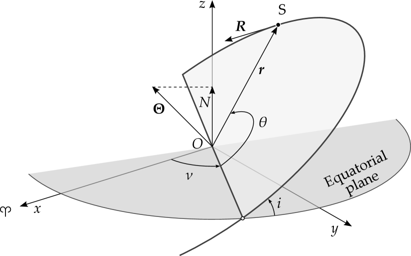
Figure 1: Polar-nodal variables $(r,\theta,\nu,R,\Theta,N)$. $r$ is the radial distance from the centre of mass of the planet to the satellite, $\theta$ is the argument of the latitude, $\nu$ represents the argument of the node, $R$ is the magnitude of the radial velocity, $\Theta$ is the magnitude of the angular momentum vector, whereas $N=\Theta\cos i$.

The main problem of the artificial satellite theory is given by the Hamiltonian

$$\mathcal{H}=\mathcal{H}_{\mathcal{K}}+\mathcal{H}_{J_{2}},$$ (2)

where $\mathcal{H}_{\mathcal{K}}$ corresponds to the Kepler problem and $\mathcal{H}_{J_{2}}$ to the influence of $J_{2}$, which is a positive constant representing the shape of the Earth-like planet. These terms, expressed in the polar-nodal variables, are:

$$\mathcal{H}_{\mathcal{K}} = \mbox{$\displaystyle\frac{1}{2}$}\left(R^{2}+\mbox{$\displaystyle\frac{\Theta^{2}}{r^{2}}$}\right)-\mbox{$\displaystyle\frac{\mu}{r}$},$$

$$\mathcal{H}_{J_{2}} = J_{2}\mbox{$\displaystyle\frac{\mu}{r}$}\left(\mbox{$\displaystyle\frac{\alpha}{r}$}\right)^{2}P_{2}(s\,\sin\theta).$$

$P_{2}$ is the Legendre polynomial of degree $2$, $\mu$ is the gravitational constant of the Earth-like planet, $\alpha$ is its equatorial radius and $s$ is the sine of the inclination $i$.

This two-degree-of-freedom problem (2-DOF) is non-integrable Irigoyen & Simó (1993). However, by applying perturbation theories, approximate analytical solutions can be obtained Kozai (1962); Brouwer (1959). Considering $J_{2}$ as a small parameter $\epsilon$, Eq. (2) can be rewritten in the form of a perturbed Hamiltonian

$$\mathcal{H}=\mathcal{H}_{0}+\epsilon\mathcal{H}_{1},$$

where $\mathcal{H}_{0}=\mathcal{H}_{\mathcal{K}}$ and $\mathcal{H}_{1}=\mathcal{H}_{J_{2}}/J_{2}$.

The perturbation theory is based on the assumption that the difference between $\mathcal{H}$ and $\mathcal{H}_{0}$ is small. Then, using the Lie transform technique, an approximate first-order closed-form analytical solution for the main problem can be developed. The elimination of the Parallax Deprit (1981) is a Lie transform, $(r,\theta,\nu,R,\Theta,N)\longrightarrow(r^{\prime},\theta^{\prime},\nu^{\prime},R^{\prime},\Theta^{\prime},N^{\prime})$, which removes the long-period terms, produced by the argument of the perigee, from the transformed Hamiltonian $\mathcal{K}$, whereas the short-period terms, caused by the mean anomaly $M$, still remain in $\mathcal{K}$ through the variables $(r,R)$. It must be noted that the argument of the latitude is the sum of the argument of the perigee and the true anomaly $f$, which is related to the mean anomaly $l$ through Kepler’s equation. Finally, the transformed Hamiltonian and the generating function of the corresponding Lie transform can be simultaneously obtained. The expression of $\mathcal{K}$ yields

$$\mathcal{K}=\mathcal{K}_{0}+\epsilon\mathcal{K}_{1},$$

where

$$\mathcal{K}_{0} = \mbox{$\displaystyle\frac{1}{2}$}\left(R^{\prime 2}+\mbox{$\displaystyle\frac{\Theta^{\prime 2}}{r^{\prime 2}}$}\right)-\mbox{$\displaystyle\frac{\mu}{r^{\prime}}$},$$

$$\mathcal{K}_{1} = \mbox{$\displaystyle\frac{\alpha^{2}\mu^{2}}{\Theta^{\prime 2}}$}\left(\mbox{$\displaystyle\frac{1}{2}$}-\mbox{$\displaystyle\frac{3}{4}$}s^{\prime 2}\right)\mbox{$\displaystyle\frac{1}{r^{\prime 2}}$}.$$

As can be observed, the argument of the latitude $\theta^{\prime}$ does not appear in the transformed Hamiltonian, which implies that the number of degrees of freedom is reduced to one and, therefore, it is trivially integrable. The direct and inverse transformations can be calculated from the generating function (see Appendix A).

Then, $\mathcal{K}$ is transformed into a perturbed harmonic oscillator by replacing the variables $r^{\prime}$, $dr^{\prime}/dt$ with two new variables $u,v$, respectively, and the time $t$ with a new independent variable $\tau$:

$$u=\mbox{$\displaystyle\frac{1}{r^{\prime}}$}-\frac{1}{p^{\prime}},\qquad r^{\prime 2}\mbox{$\displaystyle\frac{d\tau}{dt}$}=\Theta^{\prime},\qquad v=\mbox{$\displaystyle\frac{du}{d\tau}$},$$ (3)

with $p^{\prime}=\Theta^{\prime 2}/\mu$. Finally, we obtain

$$\mbox{$\displaystyle\frac{d^{2}u}{d\tau^{2}}$}+u=\epsilon\mathcal{P}\left(\frac{1}{p^{\prime}}-u\right),$$

where

$$\mathcal{P} = \-\mbox{$\displaystyle\frac{\alpha^{2}}{p^{\prime 2}}$}\left(1-\mbox{$\displaystyle\frac{3}{2}$}s^{\prime 2}\right)$$

is a constant.

Then, the Krylov-Bogoliubov-Mitropolsky method is applied to the integration of this harmonic oscillator. This method assumes an asymptotic expansion of the solution in the form

$$u=\delta\cos\psi+\displaystyle\sum_{i\geq 1}\mbox{$\displaystyle\frac{\epsilon^{i}}{i!}$}u_{i}(\delta,\psi),$$

where $u_{i}$ are $2\pi$-periodic functions in $\psi$, and the relation of $\delta$ and $\psi$ with the fictitious time $\tau$ is given by

$$\frac{d\delta}{d\tau} = \displaystyle\sum_{i\geq 0}\mbox{$\displaystyle\frac{\epsilon^{i}}{i!}$}A_{n}(\delta),$$

$$\frac{d\psi}{d\tau} = \displaystyle\sum_{i\geq 0}\mbox{$\displaystyle\frac{\epsilon^{i}}{i!}$}B_{n}(\delta).$$

The values of the first order of $u$ and $v$ are provided by the Krylov-Bogoliubov-Mitropolsky method, together with the variation of the amplitude $\delta$ and the perturbed true anomaly $\psi$ with respect to the fictitious time $\tau$:

$$\frac{d\delta}{d\tau} = 0,$$

$$\frac{d\psi}{d\tau} = 1-\frac{\epsilon}{2}\mathcal{P}.$$

Finally, the expressions of the polar nodal variables are:

$$\frac{p^{\prime}}{r^{\prime}} = 1+\delta\,p^{\prime}\cos\psi+\epsilon\mathcal{P},$$

$$(\theta^{\prime}-\theta^{\prime}_{0})\mbox{$\displaystyle\frac{d\psi}{d\tau}$} = \psi+\frac{\epsilon}{2}\left(\frac{\alpha}{p^{\prime}}\right)^{2}\left(5-6s^{\prime 2}\right)\psi,$$

$$(\nu^{\prime}-\nu^{\prime}_{0})\mbox{$\displaystyle\frac{d\psi}{d\tau}$} = -\frac{3\,\epsilon}{2}\left(\frac{\alpha}{p^{\prime}}\right)^{2}c^{\prime}\psi,$$

$$\frac{R^{\prime}}{\delta\Theta^{\prime}} = \sin\psi+\frac{\epsilon}{2}\mathcal{P}\sin\psi,$$

$$\Theta^{\prime} = \Theta^{\prime}_{0},$$

$$N^{\prime} = N^{\prime}_{0},$$

where $c^{\prime}$ is the cosine of $i^{\prime}$.

Combining the relations of $\psi$ with $\tau$, and $\tau$ with $t$, we obtain the following relation between $\psi$ and $t$:

$$r^{2}d\psi=\Theta\mbox{$\displaystyle\frac{d\psi}{d\tau}$}dt.$$ (4)

In order to integrate Eq. (4), an auxiliary variable $E_{k}$, which has a similar meaning as the eccentric anomaly in the elliptical motion, is defined by the relations

$$\cos\psi=\mbox{$\displaystyle\frac{\sqrt{1-e_{k}^{2}}\sin E_{k}}{1-e_{k}\cos E_{k}}$},\qquad\sin\psi=\mbox{$\displaystyle\frac{\cos E_{k}-e_{k}}{1-e_{k}\cos E_{k}}$},$$

where $e_{k}=\delta p^{\prime}$. After that, taking into account the relation between $u$ and $r^{\prime}$ given in Eq. (3), we obtain

$$M_{k} = E_{k}-e_{k}\sin E_{k}+\epsilon\frac{\alpha^{2}(3s^{2}-2)}{4a_{k}^{2}\left(1-e_{k}^{2}\right)^{3}}\left[2\left(e_{k}^{2}+2\right)E_{k}\right.$$

$$\left.-8e_{k}\sin E_{k}+e_{k}^{2}\sin 2E_{k}\right],$$

with

$$M_{k}=\frac{\Theta}{a_{k}\eta_{k}}\mbox{$\displaystyle\frac{d\psi}{d\tau}$}(t-T),$$ (6)

where $\eta_{k}=\sqrt{1-e_{k}^{2}}$, $a_{k}=p^{\prime}/\eta_{k}$, and the time $T$ corresponds to the instant when $\psi=0$ (see Reference San-Juan (2009) for more details). This equation can be considered a perturbed case of the classical Kepler’s equation, and it plays the same role in the accuracy determination of the position of the satellite.

It is worth noting that the values of $e_{k}$ and $a_{k}$ are close to the values of eccentricity and semi-major axis of the orbit, respectively. That is the reason why $e_{k}$ and $a_{k}$ will be approximated by the real values of eccentricity and semi-major axis. This assumption will be extended to the new anomalies $E_{k}$ and $M_{k}$, and their behaviour compared with the eccentric and mean anomalies of the orbit, $E$ and $M$, in the theoretical study of Eq. (3) that is presented in this work. Hereinafter, with a slight notation abuse, we will refer to the generalized eccentric and mean anomalies with the symbols $E$ and $M$.

4 Generalized Kepler’s equation

The first-order generalized Kepler’s equation (GKE) is given by

$$M = E-e\sin E$$

$$+\frac{\epsilon^{*}}{\left(1-e^{2}\right)^{3}}\left[2\left(e^{2}+2\right)E-8e\sin E+e^{2}\sin 2E\right],\noindent$$

where $\epsilon^{*}$ represents a new small dimensionless parameter which depends on the physical constants, $\epsilon=J_{2}$ and $\alpha$, and the generalized inclination and semi-major axis:

$$\epsilon^{*}=\epsilon\left(\frac{\alpha}{2a}\right)^{2}\left(3s^{2}-2\right).$$ (7)

Fig. 2 (a) shows a graphical representation of $\epsilon^{*}(a,i)$. The units of $a$ and $i$ are mean equatorial planet radii and radian, respectively. The sign of $\epsilon^{*}$ depends on the inclination: $\epsilon^{*}$ takes positive values for $i\in(r_{1},r_{2})$, reaching its maximum, $J_{2}/4$, when $i=\pi/2$ and $a=\alpha$, negative values for $i\in[0,r_{1})$ and $i\in(r_{2},\pi]$, reaching its minimum, $-J_{2}/2$, when $i=0$ and $a=\alpha$, and zero values for the inclinations $r_{1}=\arcsin(\sqrt{2/3})$ and $r_{2}=\pi-\arcsin(\sqrt{2/3})$, that is, the roots of the equation $\epsilon^{*}=0$. For the values $r_{1}$ and $r_{2}$, the classical KE is recovered. On the other hand, the value of $|\epsilon^{*}|$ decreases when $a$ increases. Fig. 2 (b) shows the plot of $\epsilon^{*}$ when the semi-major axis takes the value of $\alpha$ $(-J_{2}/2\leq\epsilon^{*}\leq J_{2}/4)$. Positive values of $\epsilon^{*}$ are plotted in red while negative values are in blue.

1

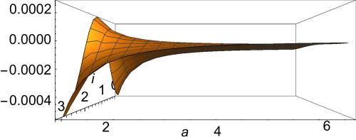
(a) $\epsilon^{*}(a,i)$.

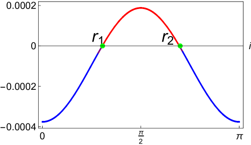
(b) $\epsilon^{*}(a=\alpha,i)$.

Figure 2: Graphical representation of $\epsilon^{*}$. The magnitude $|\epsilon^{*}|$ depends on $a$, whereas its sign is a function of $i$. In the case of the Earth, $J_{2}=0.001082626836196$, and therefore $\epsilon^{*}\in[-0.00054131341,0.000270656709]$.

Solving the perturbed Kepler’s equation in the elliptic case is equivalent to finding the zeros of the function

$$G(E) = E-e\sin E-M$$

$$+\frac{\epsilon^{*}}{\left(1-e^{2}\right)^{3}}\left[2\left(e^{2}+2\right)E-8e\sin E+e^{2}\sin 2E\right],$$

for fixed values of $e$ and $M$. This function is continuous and differentiable on $\mathbb{R}$ for each $(e,M)\in[0,1)\times\mathbb{R}$. Moreover, the perturbed Kepler’s equation, as well as the classical Kepler’s equation, is symmetric with respect to the line of apsides. However, the solutions obtained in the interval $[0,\pi]$ cannot be extended to other ranges of $E$ and $M$ because the values of $G$ are different when $E$, $M$ are replaced with $E\pm 2k\pi$, $M\pm 2k\pi$, respectively. However, $G$ is a $2\pi$-periodic function only in the eccentric anomaly $E$ for those values of the eccentricity that satisfy the relation

$$e_{p}=\sqrt{1+\frac{2\epsilon^{*}}{3^{1/3}\mathcal{R}}+\frac{\mathcal{R}}{3^{2/3}}},$$

where $\mathcal{R}=\sqrt[3]{27\epsilon^{*}+\sqrt{3}\sqrt{243{\epsilon^{*}}^{2}-8{\epsilon^{*}}^{3}}}$. Taking Eq. (4) into account, Fig. 3 (a) shows a graphical representation of $e_{p}(a,i)$. The units of $a$ and $i$ are mean equatorial planet radii and radian, respectively. $e_{p}$ only exists for $i\in[0,r_{1})\cup(r_{2},\pi]$; when $a=\alpha$, the roots of the equation $e_{p}=1$ are $r_{1}=\arcsin(\sqrt{2/3})$ and $r_{2}=\pi-\arcsin(\sqrt{2/3})$ (Fig. 3 (b)). Remember that the classical KE is recovered for the values of inclination $r_{1}$ and $r_{2}$. On the other hand, the value of $e_{p}$ increases when $a$ increases.

1

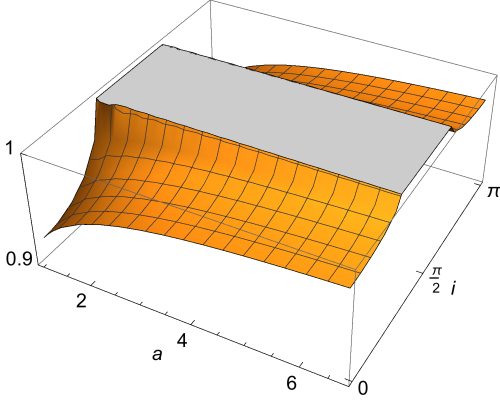
(a) $e_{p}(a,i)$.

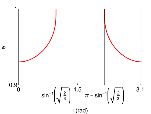
(b) $e_{p}(a=\alpha,i)$.

Figure 3: Graphical representation of $e_{p}$. The value $e_{p}$ depends on $a$, whereas its existence is a function of $i$.

In general, the solution of $G(E)=0$ is not unique in the interval $[0,\pi]$. In particular, when $i\in[0,r_{1})\cup(r_{2},\pi]$, that is, $\epsilon^{*}<0$, and $e\geq e_{p}$, the number of solutions are two, whereas for $e<e_{p}$ we only have one solution, as can be seen in Fig. 4 (a). In the particular case of $e=e_{p}$, these solutions are $E=0$ and $E=\pi$. On the other hand, when $i\in[r_{1},r_{2}]$, that is, $\epsilon^{*}\geq 0$, the function $G$ is monotone, and then the solution is unique for $0\leq e<1$. Finally, it is not possible to guarantee that for $M\in[0,\pi]$ then $E\in[0,\pi]$. Fig. 4 (b) shows all the solutions of the equation for $M=\pi$ and $a=7200$ km. The red line shows all the solutions when $\epsilon^{*}<0$; as can be seen, the solutions are out of the interval $[0,\pi]$. For high values of the eccentricity, the value of the solution increases, that is, the solution moves away from the interval. The black line, which corresponds to $\epsilon^{*}=0$, represents the classical KE, in which case whenever $M=\pi$, the solutions are $E=\pi$ for any eccentricity. Finally, the blue line corresponds to $\epsilon^{*}>0$, case in which all the solutions are contained in the interval $[0,\pi]$. In the case of $M=0$, part of the solutions are out of the interval only for negative values of $\epsilon^{*}$ and $e<e_{p}$.

1

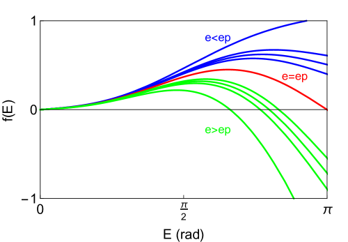
(a) $G$ plots for $i_{1}=0$ rad, that is, $\epsilon^{*}<0$, $M=0$ rad and several high values of eccentricity.

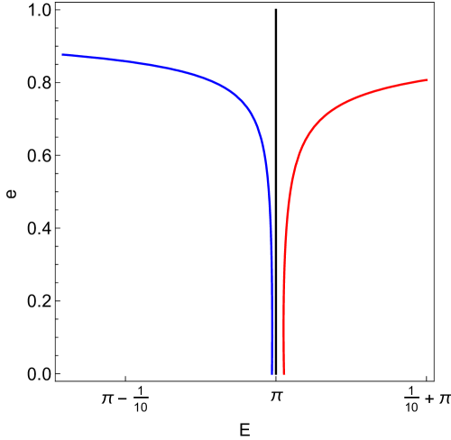
(b) Solutions of $G$ for $M=\pi$ and $0\leq e<1$.

Figure 4: Graphical representations for $a=7200$.

5 Numerical Results

In this section, the Danby method (DM) and three initial guesses are applied so as to solve the GKE. It is worth noting that, in order to solve Eq. (4) with this iterative method, it is necessary to calculate the first, second and third derivatives of $G$ with respect to $E$,

$$G^{\prime}(E) = 1-e\cos E+\frac{2\epsilon^{*}}{\left(1-e^{2}\right)^{3}}\left[\left(e^{2}+2\right)\right.$$

$$\left.-4e\cos E+e^{2}\cos 2E\right],$$

$$G^{\prime\prime}(E) = e\sin E+\frac{4e\epsilon^{*}}{\left(1-e^{2}\right)^{3}}\left[2\sin E-e\sin 2E\right],$$

$$G^{\prime\prime\prime}(E) = e\cos E+\frac{8e\epsilon^{*}}{\left(1-e^{2}\right)^{3}}\left[\cos E-e\cos 2E\right].$$

Table 1 shows the initial guesses used in our study. The first two ones have been proposed in scientific literature for solving KE: $S_{1}$ is a classical and simple function of M, whereas in $S_{2}$ the computation is divided into two regions (see Reference Danby & Burkardt (1983) for more details). Finally, $S_{3}$ is the solution of Kepler’s equation itself, which is also calculated using the Danby method.

Table 1: Initial guesses used to solve the GKE.

Id	$E_{0}$
$S_{1}$	$M$
$S_{2}$	$M+e^{2}(\sqrt[3]{6M}-M)$	if $M<0.1$
	$M+0.85e$	if $M\geq 0.1$
$S_{3}$	$\mathrm{solution\>of\>KE}$

Then, this iterative method is used to solve the GKE for a grid of points in the $M$–$e$ plane ($0\leq M\leq\pi$, $0\leq e<1$), separated by a uniform space of $\Delta M=1/1000$ rad and $\Delta e=1/1000$; the number of points in the grid is therefore $3142000$. It is worth noting that this study is restricted to the interval $M\in[0,\pi]$ because, in our problem, the GKE appears as a perturbed case of the KE, although an extensive analysis should be done for all $\mathbb{R}$ from the mathematical point of view.

The maximum number of iterations allowed is 20, and the convergence is considered to be achieved if $\|E_{i+1}-E_{i}\|\leq 10^{-14}$. The selected planet is the Earth, for which five different inclinations are compared. The first two values, $i_{1}=0^{\circ}$ and $i_{2}=53^{\circ}$, correspond to negative values of $\epsilon^{*}$, the third value is $r_{1}$, where the GKE is reduced to KE, and the last two values are $i_{4}=55^{\circ}$ and $i_{5}=90^{\circ}$, which correspond to positive values of $\epsilon^{*}$. On the other hand, several semi-major axes have been considered in this study, although in the following discussion the semi-major axis has been set to $7200$ km, which corresponds to a LEO orbit. Finally, an additional convergence criterion is required to determine the relation between the generalized anomalies $E$ and $M$; the iterative method converges if the root of Eq. (4) belongs to the interval $[0,\pi]$. The results of this study are summarized in figures 5-8, in which the $M$–$e$ plane has been divided into regions that correspond to the same number of iterations during the resolution of the equation. The number of points plotted in each graph is 628400.

Fig. 5 shows the results of the application of DM with the initial guesses $S_{1}$ and $S_{2}$ in the case in which GKE is reduced to KE, that is, for the value of the inclination $i_{3}=r_{1}$. In both cases, the method always converges and needs between 3 and 4 iterations for $95.91\%$ of the cases when $S_{1}$ is used, and between 2 and 3 iterations ($93.36\%$) for $S_{2}$. For more details regarding the full analysis of this combination, see References Danby & Burkardt (1983); Danby (1987).

2

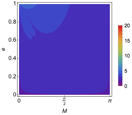
(a) $S_{1}$.

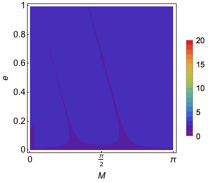
(b) $S_{2}$.

Figure 5: The colour scale shows the number of iterations of the Danby method for the value of inclination $i_{3}=r_{1}$ ($\epsilon^{*}=0$) using $S_{1}$ and $S_{2}$ as initial guesses. The method always converges in both cases. $S_{1}$ needs between 3 and 4 iterations in $95.91\%$ of the cases, whereas $S_{2}$ only needs between 2 and 3 iterations in $93.36\%$ of the cases.

Fig. 6 shows the results of the application of DM with the initial guess $S_{1}$. The case $\epsilon^{*}<0$ is illustrated in Figs. 6 (a) and (b). Most of the cases converge to the solution using between 4 and 5 iterations, with percentages of $87.44\%$ for $i_{1}=0^{\circ}$ and $93.04\%$ for $i_{2}=53^{\circ}$. It is worth noting that there are non-convergent regions (red colour in Figures); these regions reach their maximum size ($10.48\%$ of the cases) for $i_{1}=0^{\circ}$, and decrease as the inclination increases, until they disappear for $i_{3}=r_{1}$. For $i_{2}=53^{\circ}$ the non-convergent region represents $3.58\%$ of the cases, and corresponds to values $(e,M)$ that cause GKE to have two solutions or one solution out of the interval $[0,\pi]$. Figs. 6 (c) and (d) correspond to $\epsilon^{*}>0$: the cases that converge to the solution using between 3 and 4 iterations are $95.63\%$ for $i_{4}=55^{\circ}$ and $94.22\%$ for $i_{5}=90^{\circ}$. It is worth noting that the method has convergence problems for very high eccentricities $e>0.99$. The change in the shape of the regions in the $M$–$e$ plane with respect to the KE case can be seen for high eccentricities ($e>0.9$).

2

(a) $i_{1}=0^{\circ}$.

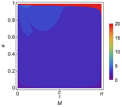
(b) $i_{2}=53^{\circ}$.

(c) $i_{4}=55^{\circ}$.

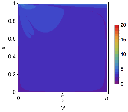
(d) $i_{5}=90^{\circ}$.

Figure 6: The colour scale shows the number of iterations of the Danby method using $S_{1}$ as initial guess. $\epsilon^{*}$ takes negative values for $i_{1}$ and $i_{2}$, and positive values for $i_{4}$ and $i_{5}$. The red colour represents non-convergent regions. Most of the cases require between 4 and 5 iterations to converge to the solution for $i_{1}$ and $i_{2}$, with percentages of $87.44\%$ and $93.04\%$ respectively, whereas the number of iterations practically reduces by one for $i_{4}$ and $i_{5}$, with percentages of $95.63\%$ and $94.22\%$, respectively.

The results of the application of DM with the initial guess $S_{2}$ are given in Fig. 7 and Table 2. The case $\epsilon^{*}<0$ is shown in Figs 7 (a) and (b). The size of the non-convergent regions is the same as in the cases corresponding to the use of $S_{1}$ as the initial guess. DM uses between 2 and 3 iterations in $89.25\%$ and $96.35\%$ of the cases for $i_{1}=0^{\circ}$ and $i_{2}=53^{\circ}$, respectively. Finally, Figs 7 (c) and (d) analyse the case $\epsilon^{*}>0$. DM uses between 2 and 3 iterations in $99.86\%$ and $98.63\%$ of the cases for $i_{4}=55^{\circ}$ and $i_{5}=90^{\circ}$, respectively. The method also has convergence problems for very high eccentricities, $e>0.99$. The change in the shape of the regions in the $M$–$e$ plane with respect to the KE case is also present for high eccentricities ($e>0.9$).

Table 2: Percentage of cases that require 2 or 3 iterations, when the Danby method is applied to the inclinations $0^{\circ}$, $53^{\circ}$, $55^{\circ}$ and $90^{\circ}$, for both S2 and S3 as the initial guess.

Inclination	Initial Guess	2 iterations	3 iterations
$i_{1}=0^{\circ}$	$S_{2}$	$\phantom{0}6.31\%$	$82.94\%$
	$S_{3}$	$50.27\%$	$38.98\%$
$i_{2}=53^{\circ}$	$S_{2}$	$\phantom{0}6.57\%$	$89.78\%$
	$S_{3}$	$86.87\%$	$\phantom{0}9.47\%$
$i_{3}=55^{\circ}$	$S_{2}$	$\phantom{0}6.50\%$	$93.36\%$
	$S_{3}$	$93.38\%$	$\phantom{0}5.54\%$
$i_{4}=90^{\circ}$	$S_{2}$	$\phantom{0}6.58\%$	$92.05\%$
	$S_{3}$	$66.85\%$	$28.48\%$

2

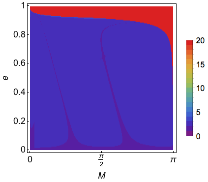
(a) $i_{1}=0^{\circ}$.

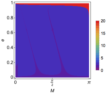
(b) $i_{2}=53^{\circ}$.

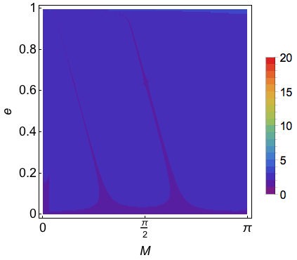
(c) $i_{4}=55^{\circ}$.

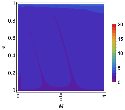
(d) $i_{5}=90^{\circ}$.

Figure 7: The colour scale shows the number of iterations of the Danby method using $S_{2}$ as initial guess. $\epsilon^{*}$ takes negative values for $i_{1}$ and $i_{2}$, and positive values for $i_{4}$ and $i_{5}$. The red colour represents non-convergent regions. Most of the cases require between 2 and 3 iterations to converge to the solution for the four inclinations $i_{1}$, $i_{2}$, $i_{3}$ and $i_{4}$, with percentages of $89.25\%$, $96.35\%$, $99.86\%$ and $98.63\%$, respectively.

To conclude this study, the solution of KE, $S_{3}$, is used as the initial guess for the Danby method. It is an intuitive initial guess due to the fact that GKE can be considered as a perturbed version of KE. The results are given in Fig. 8. The non-convergent regions for the case $\epsilon^{*}<0$ represent the same percentages as when $S_{1}$ and $S_{2}$ are taken as initial guesses. $S_{3}$ achieves convergence to the solution in only 2 iterations in more than $50\%$ of the cases, as can be seen in Table 2; this percentage increases up to $85$–$100\%$ when the inclination takes values close to $r_{1}$, for which the GKE is reduced to KE. In summary, DM requires between 2 and 3 iterations in $89.25\%$, $96.34\%$, $98.92\%$ and $95.33\%$ of the cases for $i_{1}=0^{\circ}$, $i_{2}=53^{\circ}$, $i_{4}=55^{\circ}$ and $i_{5}=90^{\circ}$, respectively. DM also has convergence problems for $e>0.99$ in the case $\epsilon^{*}>0$.

2

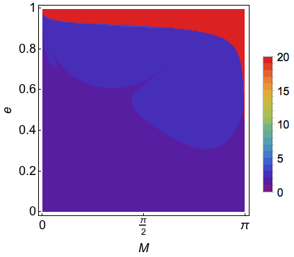
(a) $i_{1}=0^{\circ}$.

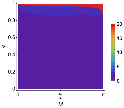
(b) $i_{2}=53^{\circ}$.

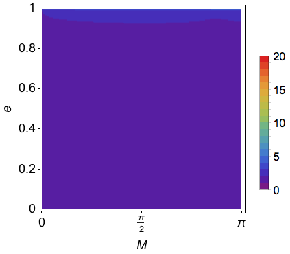
(c) $i_{4}=55^{\circ}$.

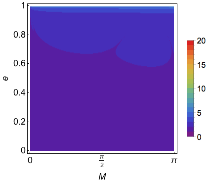
(d) $i_{5}=90^{\circ}$.

Figure 8: The colour scale shows the number of iterations of the Danby method using $S_{3}$ as initial guess. $\epsilon^{*}$ takes negative values for $i_{1}$ and $i_{2}$ and positive values for $i_{4}$ and $i_{5}$. The red colour represents non-convergent regions. The number of cases that require between 2 and 3 iterations to converge to the solution represent $50.27\%$, $86.87\%$, $93.38\%$ and $66.85\%$ for the inclinations $i_{1}$, $i_{2}$, $i_{3}$ and $i_{4}$, respectively.

As it has already been mentioned in the previous section, the value of $|\epsilon^{*}|$ decreases, and, therefore also its influence, when $a$ increases. This implies that the size of the non-convergent regions will be smaller, and the shape of the $M$–$e$ plane solutions for GKE will be similar to KE for high eccentricities.

The best computational time needed to achieve a convergence error of $10^{-14}$ with the Danby method is obtained with $S_{2}$ (red circle), whereas the worst is reached with $S_{3}$ (blue square), as can be seen in Fig 9. In particular, $S_{2}$ is approximately $20\%$ faster than $S_{3}$ for all the inclinations considered in this study. The CPU used has been an Intel Core i7 with a clock frequency of 1.7 GHz.

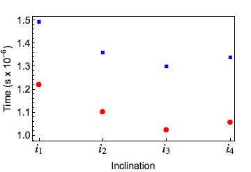
Figure 9: Computational time required to reach an error of $10^{-14}$ with the Danby method. Red circle and blue square represent the initial guesses $S_{2}$ and $S_{3}$, respectively.

6 Conclusion

In this work, a first approach to the problem of solving the generalized Kepler’s equation by using an iterative method proposed by Danby and Burkardt, together with two habitual initial guesses Danby & Burkardt (1983) used to solve Kepler’s equation, $S_{1}$ and $S_{2}$, and even with the solution of KE itself as an initial guess for GKE, $S_{3}$, has been tested. At first order, GKE is a function of the eccentricity, the mean and eccentric anomalies, and a small parameter, $\epsilon^{*}$, which depends on the semi-major axis, the inclination and the physical parameters $\alpha$ and $J_{2}$. The value of the small parameter $\epsilon^{*}$ can be negative, zero or positive: its sign is a function of the inclination, whereas its magnitude $|\epsilon^{*}|$ decreases when $a$ increases. On the other hand, when $\epsilon^{*}=0$, GKE is reduced to KE.

For the initial guesses $S_{1}$ and $S_{2}$, the behaviour of the iterative method, when GKE is solved, is similar to the KE case for $e<0.9$. For high eccentricities, $e>0.9$, the behaviour changes and non-convergent regions appear for $\epsilon^{*}<0$; in these regions we can simultaneously find convergence problems of the iterative method, multiple solutions of GKE for a value of the eccentricity $e_{p}$, and solutions that are not contained in the interval $[0,\pi]$, property that KE verifies. On the other hand, $S_{2}$ and $S_{3}$ achieve convergence to the solution in only 2 or 3 iterations in more than $90\%$ of the cases, increasing the number of iterations when the eccentricity grows. However, $S_{3}$ only needs 2 iterations to achieve convergence to the solution in more than $50\%$ of the cases; this percentage increases up to $85$–$100\%$ when the inclination takes values close to $r_{1}$ for which the GKE is reduced to KE. It is worth noting that the decrease of the number of iterations is at the expense of speed, $S_{3}$ is approximately $20\%$ slower than $S_{2}$ for all the inclinations considered in this study.

Appendix A Generating function

The first-order generating function of the elimination of the parallax is given by

$$\mathcal{W} = \left(\mbox{$\displaystyle\frac{\alpha}{p^{\prime}}$}\right)^{2}\mbox{$\displaystyle\frac{\Theta^{\prime}}{8}$}\left[S^{\prime}(4-9s^{\prime 2})\cos\theta^{\prime}+S^{\prime}s^{\prime 2}\cos 3\theta^{\prime}\right.$$

$$\qquad\qquad\left.\phantom{-}+C^{\prime}(-4+3s^{\prime 2})\sin\theta^{\prime}-3s^{\prime 2}\sin 2\theta^{\prime}\right.$$

$$\qquad\qquad\left.\phantom{-}-C^{\prime}s^{\prime 2}\sin 3\theta^{\prime}\right],$$

where $p^{\prime}=\Theta^{\prime 2}/\mu$, and $C^{\prime}$, $S^{\prime}$ are given as functions of polar-nodal variables by

$$C^{\prime} = \left(\frac{p^{\prime}}{r^{\prime}}-1\right)\cos\theta^{\prime}+\frac{p^{\prime}R^{\prime}}{\Theta^{\prime}}\sin\theta^{\prime},$$

$$R^{\prime} = \left(\frac{p^{\prime}}{r^{\prime}}-1\right)\sin\theta^{\prime}-\frac{p^{\prime}R^{\prime}}{\Theta^{\prime}}\cos\theta^{\prime}.$$

References

- Abad et al. (2001) Abad A., San-Juan J. F., Gavín A., 2001, Celestial Mechanics and Dynamical Astronomy, 79, 277
- Brouwer (1959) Brouwer D., 1959, The Astronomical Journal, 64, 378
- Caballero (1975) Caballero J. A., 1975, PhD thesis, University of Zaragoza, Spain
- Calvo (1971) Calvo M., 1971, PhD thesis, University of Zaragoza, Spain
- Colwell (1993) Colwell P., 1993, Solving Kepler’s Equation Over Three Centuries. Willmann-Bell, Richmond, VA, USA
- Danby (1987) Danby J. M. A., 1987, Celestial Mechanics, 40, 303
- Danby & Burkardt (1983) Danby J. M. A., Burkardt T. M., 1983, Celestial Mechanics, 31, 95
- Deprit (1979) Deprit A., 1979, Celestial Mechanics, 20, 325
- Deprit (1981) Deprit A., 1981, Celestial Mechanics, 24, 111
- Fukushima (1996) Fukushima T., 1996, The Astronomical Journal, 112, 2858
- Irigoyen & Simó (1993) Irigoyen M., Simó C., 1993, Celestial Mechanics and Dynamical Astronomy, 55, 281
- Kozai (1962) Kozai Y., 1962, The Astronomical Journal, 67, 446
- Krylov & Bogoliubov (1943) Krylov N. M., Bogoliubov N. N., 1943, Introduction to Non-linear Mechanics. Princeton University Press, Princeton, NJ, USA
- Lynden-Bell (2015) Lynden-Bell D., 2015, Monthly Notices of the Royal Astronomical Society, 447, 363
- Ng (1979) Ng E. W., 1979, Celestial Mechanics, 20, 243
- Nijenhuis (1991) Nijenhuis A., 1991, Celestial Mechanics and Dynamical Astronomy, 51, 319
- Odell & Gooding (1986) Odell A. W., Gooding R. H., 1986, Celestial Mechanics, 38, 307
- Palacios (2002) Palacios M., 2002, Journal of Computational and Applied Mathematics, 138, 335
- Plummer (1906) Plummer H. C., 1906, Monthly Notices of the Royal Astronomical Society, 67, 67
- Raposo-Pulido & Pel·ez (2017) Raposo-Pulido V., Pel·ez J., 2017, Monthly Notices of the Royal Astronomical Society, 467, 1702
- San-Juan (1994) San-Juan J. F., 1994, Technical Report CT/TI/MS/MN/94-250, ATESAT: automatization of theories and ephemeris in the artificial satellite problem. Centre National d’Études Spatiales (CNES), Toulouse, France
- San-Juan (2009) San-Juan J. F., 2009, Advances in the Astronautical Sciences, 134, 653
- San-Juan & Serrano (2000) San-Juan J. F., Serrano S., 2000, Technical Report DTS/MPI/MS/MN/2000-057, Application of the Z6PPKB ATESAT-model to compute the orbit of an artificial satellite around Mars. Centre National d’Études Spatiales (CNES), Toulouse, France
- San-Juan et al. (2011) San-Juan J. F., Gavín A., López L. M., López R., 2011, The Journal of the Astronautical Sciences, 58, 643
- See (1895) See T. J. J., 1895, Monthly Notices of the Royal Astronomical Society, 56, 54
- Smith (1979) Smith G. R., 1979, Celestial Mechanics, 19, 163
- Taff & Brennan (1989) Taff L. G., Brennan T. A., 1989, Celestial Mechanics and Dynamical Astronomy, 46, 163
- Traub (1982) Traub J. F., 1982, Iterative Methods for the Solution of Equations, second edn. Chelsea Publishing Company, New York, NY, USA