Modelling Phase Separation In Amorphous Solid Dispersions

Abstract

Much work has been devoted to analysing thermodynamic models for solid dispersions with a view to identifying regions in the phase diagram where amorphous phase separation or drug recrystallization can occur. However, detailed partial differential equation non-equilibrium models that track the evolution of solid dispersions in time and space are lacking. Hence theoretical predictions for the timescale over which phase separation occurs in a solid dispersion are not available. In this paper, we address some of these deficiencies by (i) constructing a general multicomponent diffusion model for a dissolving solid dispersion; (ii) specializing the model to a binary drug/polymer system in storage; (iii) deriving an effective concentration dependent drug diffusion coefficient for the binary system, thereby obtaining a theoretical prediction for the timescale over which phase separation occurs; (iv) calculating the phase diagram for the Felodipine/HPMCAS system; and (iv) presenting a detailed numerical investigation of the Felodipine/HPMCAS system assuming a Flory-Huggins activity coefficient. The numerical simulations exhibit numerous interesting phenomena, such as the formation of polymer droplets and strings, Ostwald ripening/coarsening, phase inversion, and droplet-to-string transitions. A numerical simulation of the fabrication process for a solid dispersion in a hot melt extruder was also presented.

Keywords: amorphous solid dispersion, phase separation, mathematical model, drug diffusion

1 Introduction

Drugs that are delivered orally via a tablet should ideally be readily soluble in water. Drugs that are poorly water-soluble tend to pass through the gastrointestinal tract before they can fully dissolve, and this typically leads to poor bioavailability of the drug. Unfortunately, many drugs currently on the market or in development are poorly water-soluble, and this presents a serious challenge to the pharmaceutical industry. Many strategies have been developed to improve the solubility of drugs, such as the use of surfactants, cocrystals, lipid-based formulations, and particle size reduction. The literature on this topic is extensive, and recent reviews can be found in [1, 2, 3].

One particularly effective strategy to improve drug solubility is to use a solid dispersion [4, 5, 6]. A solid dispersion typically consists of a hydrophobic drug embedded in a hydrophilic polymer [7, 8] matrix, where the matrix can be either in the amorphous or crystalline state. The drug is preferably in a molecularly dispersed state, but may also be present in amorphous particles or even in the crystalline form (though this is usually undesirable); see Figure 1. The drug release concept for most solid dispersions is based on the so-called spring and parachute effect [9]. When the drug and the hydrophilic polymer dissolve in solution, a supersaturated drug solution is quickly created (the spring). Although the drug concentration then subsequently decreases, the rate of decrease is slowed by drug-polymer interactions in the dispersion, so that the drug can be present at supersaturated levels in the solution for a period of some hours (the parachute). This results in improved bioavailability of the drug when the solid dispersion dosage form is taken orally.

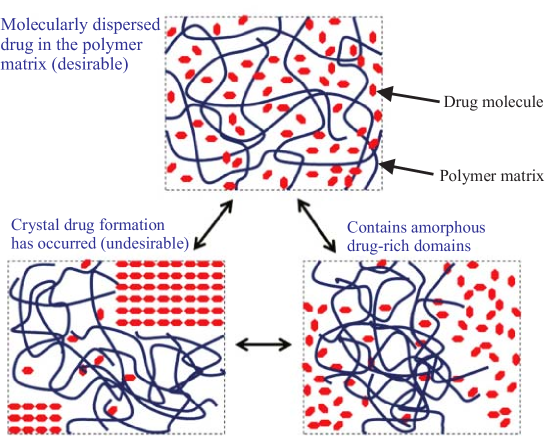
Figure 1: Adapted from [5]. In this figure, we show three possible structures for a polymer/drug dispersion. Top: Here the drug is in the molecularly dispersed state, which is usually desirable for a solid dispersion. Bottom left: Here the dispersion contains drug in the crystalline form. Bottom right: Here the dispersion contains amorphous drug-rich domains.

Drug loading in most dispersions greatly exceeds the equilibrium solubility in the polymer matrix for typical storage temperatures. Hence these systems are usually unstable, with phase separation eventually occurring [5]. In such cases, the drug will eventually crystallise out or form an amorphous phase separation. However, if the dispersion is stored well below the glass transition temperature [10] for the polymer, and is kept dry, this can happen extremely slowly. The system is then for all practical purposes stable, and is said to be metastable. The humidity of the storage environment can be an issue because even small amounts of moisture can significantly affect the glass transition temperature. Hence polymers that have high glass transition temperatures and that are resistant to water absorption have become popular. An example of one such polymer is Hydroxypropyl Methylcellulose Acetate Succinate (HPMCAS).

Phase separation of solid dispersions in storage is clearly undesirable from the point of manufacturers. Hence much work has been devoted to constructing phase diagrams for solid dispersions with a view to identifying regimes where drug recrystallization or amorphous phase separation can occur. These phase diagrams are constructed with the aid of thermodynamic models. The most widely used thermodynamic model in this context is the Flory-Huggins model [11, 12, 13] for polymer solutions.

Flory-Huggins theory is a lattice-based model in which the drug and polymer are confined to live on a regular lattice. Flory-Huggins theory is an extension of regular solution theory, as explained in Chapter 7 of [13]. In the context of a drug/polymer system, each drug molecule is taken to occupy one lattice site and each polymer segment is taken to occupy $m\gg 1$ sites. Under a number of further simplifying assumptions [13], the change in entropy and enthalpy associated with the mixing of the polymer and drug are calculated. With these in hand, the change in bulk Gibbs free energy ($\Delta g_{b}^{mix}$) per mole associated with mixing is readily calculated, and is found to be

$$\frac{\Delta g_{b}^{mix}}{RT}=X_{d}\ln(\phi_{d})+X_{p}\ln(\phi_{p})+\chi_{dp}X_{d}\phi_{p},$$ (1)

where $R$ is the gas constant, $T$ is the temperature, $X_{d},X_{p}=1-X_{d}$ are the mole fractions of the drug and polymer, respectively, and $\phi_{d},\phi_{p}$ are the volume fractions of the drug and polymer, respectively. The quantity $\chi_{dp}$ is referred to as the Flory-Huggins interaction parameter, and it is discussed further below. The mole fractions and volume fractions are related via the formulae

$$\phi_{d}=\frac{X_{d}}{X_{d}+mX_{p}},\hskip 9.95863pt\phi_{p}=\frac{mX_{p}}{X_{d}+mX_{p}}.$$ (2)

When the model is applied to real binary systems, $m$ can be calculated using the formula

$$m=\frac{V_{p}}{V_{d}}$$ (3)

where $V_{p}$, $V_{d}$ (molar^-1) are the molar volumes of the polymer and drug, respectively.

The mixing of the polymer and drug is spontaneous if $\Delta G_{mix}<0$. The Flory-Huggins parameter $\chi_{dp}$ takes the form

$$\chi_{dp}=\rho^{2}\left(w_{dp}-\frac{w_{dd}+w_{pp}}{2}\right)$$ (4)

where $\rho^{2}$ is a positive parameter, and $w_{dp}$, $w_{dd}$, $w_{pp}$ give measures of the drug-polymer, drug-drug and polymer-polymer interaction energy, respectively. If $\chi_{dp}<0$ then $w_{dp}<(w_{dd}+w_{pp})/2$ indicating that that the mixed state has lower energy than the separated pure states, so that mixing is favoured. Conversely, $\chi_{dp}>0$ is indicative of demixing being favoured. However, these statements are indicative rather than precise, as will be explained in Section 3. We should also note that $\chi_{dp}$ is temperature dependent, and is usually given the empirical form

$$\chi_{dp}(T)=\frac{\alpha}{T}+\beta$$ (5)

where $\alpha,\beta$ are constants.

Flory-Huggins theory has frequently been used to analyse the stability of binary solid dispersion systems in storage; see, for example, [14, 15, 16, 17, 18, 19, 20, 21, 22, 23]. In many of these studies, the Flory-Huggins interaction parameter is first estimated using the melting point depression method [24], or using the Hildebrand and Scott method [25], which involves the estimation of solubility parameters. Once estimates for $\chi_{dp}(T)$ have been obtained, the Gibbs free energy of mixing $\Delta G_{mix}$ can be calculated, which in turn enables the construction of phase diagrams for the systems. Phase diagrams assist with the identification of regions in composition-temperature space where the system is prone to recrystallization or amorphous phase separation.

The models we shall develop in the current study are generic and are not tied to making a specific choice of statistical model. However, given the particular importance of Flory-Huggins theory in applications, we shall derive detailed results for this case. Also, all of our numerical illustrations are calculated within the context of Flory-Huggins theory. It should be emphasized that Flory-Huggins theory does involve quite a number of simplifying assumptions which are not appropriate for some systems; see [26] for a recent critique of the model.

2 Theoretical formulation

2.1 A multicomponent diffusion model for solid dispersions

We develop a multicomponent diffusion model for the evolution of the concentrations of the components constituting a solid dispersion. We suppose for the moment that there are $p$ components. However, in the analysis we shall consider in the current study, we will in fact have $p=2$, with one of the components being the polymer, and the other being the drug. For a dissolving solid dispersion, there are three components $p=3$: the polymer, the drug, and the solvent.

The chemical potential $\mu_{i}$ (J/mole) of species $i$ $(i=1,2,...,p)$ gives the Gibbs free energy per mole of species $i$, and is given here by ([27])

$$\mu_{i}=\mu_{i}^{b}-\epsilon_{i}^{2}\nabla^{2}X_{i}$$ (6)

where

$$\mu_{i}^{b}=\mu_{i}^{0}+RT\ln(a_{i})$$ (7)

and where $\mu_{i}^{b}$ is the bulk chemical potential of species $i$, $\mu_{i0}$ is the chemical potential of species $i$ in the pure state, $a_{i}$ is the activity of species $i$, and the term involving $\epsilon_{i}^{2}>0$ (m²J/mole) penalises the formation of phase boundaries ([28], [29],[30], [31], [32]). The parameters $\epsilon_{i}^{2}$ are referred to as gradient energy coefficients ([33], [34]). Here $X_{i}$ is the molar fraction of species $i$ ($i=1,2,...,p$), and the activities can depend on these molar fractions, so that

$$a_{i}=a_{i}(X_{1},X_{2},...,X_{p}).$$

The molar fraction is related to the molar concentration via

$$X_{i}=V_{i}c_{i}$$ (8)

where $V_{i}$ (molar^-1) is the molar volume of species $i$. The flux of species $i$ (molar$\cdot$m/s) is given by

$${\bf J}_{i}=c_{i}{\bf v}_{i}$$ (9)

where $c_{i}$ (molar), ${\bf v}_{i}$ (m/s) give the molar concentration and drift velocity, respectively, of species $i$. The drift velocity ${\bf v}_{i}$ gives the average velocity a particle of species $i$ attains due to the diffusion force acting on it, and is given here by

$${\bf v}_{i}=M_{i}{\bf{\cal F}}_{i}=-M_{i}\nabla\mu_{i}$$ (10)

where $M_{i}$ (mole$\cdot$s/kg), ${\bf{\cal F}}_{i}$ (J/[m$\cdot$mole]) give the mobility and diffusion force, respectively, for species $i$. Equations (9) and (10) give

$${\bf J}_{i}=-M_{i}c_{i}\nabla\mu_{i}.$$ (11)

Conservation of mass for species $i$ implies that

$$\frac{\partial c_{i}}{\partial t}+\nabla\cdot{\bf J}_{i}=0$$ (12)

and using (11) now gives

$$\frac{\partial c_{i}}{\partial t}=\nabla\cdot\left(M_{i}c_{i}\nabla\mu_{i}\right)$$

or equivalently

$$\frac{\partial X_{i}}{\partial t}=\nabla\cdot\left(D_{i}X_{i}\nabla\left\{\frac{\mu_{i}-\mu_{i}^{0}}{RT}\right\}\right)$$ (13)

with

$$\frac{\mu_{i}-\mu_{i}^{0}}{RT}=\ln(a_{i})-\delta_{i}^{2}\nabla^{2}X_{i}$$ (14)

for $i=1,2,...,p$, and where $\delta_{i}^{2}=\epsilon_{i}^{2}/RT>0$ (m²/molar), and

$$D_{i}=M_{i}RT\hskip 28.45274pt\mbox{(Einstein relation)}$$

is the self-diffusion coefficient for species $i$.

The model formulation given by (13) and (14) based on chemical potentials will be used for the numerical scheme described in Section 4. However, it is also of value to develop a formulation involving diffusion coefficients since these yield immediate information regarding timescales for transport processes, and will also the enable the development of analytical results via a linearization process.

Diffusion Coefficients

Using (6), (7) and (11) gives

$${\bf J}_{i}=-M_{i}c_{i}\nabla\mu_{i}=-M_{i}c_{i}\left(\frac{RT}{a_{i}}\nabla a_{i}-\epsilon_{i}^{2}\nabla(\nabla^{2}X_{i})\right)$$

and then using the fact that the activities depend on the molar fractions gives

$${\bf J}_{i}=-M_{i}c_{i}\left(\frac{RT}{a_{i}}\sum_{j=1}^{p}\frac{\partial a_{i}}{\partial X_{j}}\nabla X_{j}-\epsilon_{i}^{2}\nabla(\nabla^{2}X_{i})\right).$$ (15)

Using (8), we can now write (15) as

$${\bf J}_{i}=-\sum_{j=1}^{p}D_{ij}\nabla c_{j}+D_{i}\varepsilon_{i}^{2}c_{i}\nabla(\nabla^{2}c_{i})$$ (16)

where $\varepsilon_{i}^{2}=V_{i}\delta_{i}^{2}$ and where the diffusion coefficients $D_{ij}$ (m²/s) are given by

$$D_{ij}=D_{i}\frac{V_{j}}{V_{i}}\frac{X_{i}}{a_{i}}\frac{\partial a_{i}}{\partial X_{j}}.\hskip 28.45274pti,j=1,2,...,p$$ (17)

Conservation of mass (12) then implies that (reverting to molar fractions)

$$\frac{\partial X_{i}}{\partial t}=\nabla\cdot\left(\sum_{j=1}^{p}\frac{V_{i}}{V_{j}}D_{ij}({\bf X})\nabla X_{j}-D_{i}\delta_{i}^{2}X_{i}\nabla(\nabla^{2}X_{i})\right)\hskip 28.45274pti=1,2,...,p$$ (18)

where ${\bf X}=(X_{1},X_{2},...,X_{p})$, and where we have included the concentration dependence of the diffusion coefficients $D_{ij}$ here to emphasise that this system is in general a coupled system of nonlinear diffusion equations. It should benoted that the equations (18) are not independent since $\sum_{i=1}^{p}X_{i}=1$, and so it is sufficient to solve for $p-1$ concentrations only.

2.2 Activity coefficients

The activities $a_{i}$ are usually written as

$$a_{i}=\gamma_{i}X_{i}$$

where the $\gamma_{i}=\gamma_{i}(X_{1},X_{2},...,X_{p})$ are referred to as activity coefficients. Equations (17) now give

$$D_{ij}=D_{i}\frac{V_{j}}{V_{i}}\left(\delta_{ij}+\frac{X_{i}}{\gamma_{i}}\frac{\partial\gamma_{i}}{\partial X_{j}}\right)\hskip 28.45274pti,j=1,2,...,p$$ (19)

where $\delta_{ij}$ is the Kronecker delta.

The details of the interactions between the species in solution are captured in the modelling by choosing appropriate forms for the activity coefficients $\gamma_{i}=\gamma_{i}(X_{1},X_{2},...,X_{p})$. The construction of appropriate forms for the $\gamma_{i}$ for various solutions is a large subject with a large literature; see, for example, the books [35] and [36].

2.3 The storage problem for a binary mixture

In the current study, we shall be modelling the behaviour of solid dispersions in storage. In this case, we have $p=2$, with the label 1 referring to the drug and the label 2 referring to the polymer. However, for transparency, we choose here to use the labels $d,p$ rather than $1,2$, where $d$ stands for drug, and $p$ for polymer. Then using (18) and the fact that $X_{p}=1-X_{d}$, we have

$$\frac{\partial X_{d}}{\partial t}=\nabla\cdot\left\{D_{\mbox{\scriptsize eff}}(X_{d})\nabla X_{d}-D_{d}\delta_{d}^{2}X_{d}\nabla\left(\nabla^{2}X_{d}\right)\right\}.$$ (20)

where the effective concentration-dependent diffusion coefficient for the drug in the solid dispersion is

$$D_{\mbox{\scriptsize eff}}(X_{d})=D_{dd}(X_{d})-V_{d}D_{dp}(X_{d})/V_{p}=D_{d}\left\{1+\frac{X_{d}}{\gamma_{d}}\left[\frac{\partial\gamma_{d}}{\partial X_{d}}-\frac{\partial\gamma_{d}}{\partial X_{p}}\right]\right\}.$$ (21)

For the particular case of a binary Flory-Huggins theory (see Section 1), the activity coefficients are given by

$$\ln(\gamma_{d})=\ln\left(\frac{\phi_{d}}{X_{d}}\right)+1-\frac{\phi_{d}}{X_{d}}+\chi_{dp}\phi_{p}^{2},$$ (22)

$$\ln(\gamma_{p})=\ln\left(\frac{\phi_{p}}{X_{p}}\right)+1-\frac{\phi_{p}}{X_{p}}+m\chi_{dp}\phi_{d}^{2},$$ (23)

where the volume fractions $\phi_{d},\phi_{p}$ are given by (2). Substituting (22) in (21) gives

$$D_{\mbox{\scriptsize eff}}(X_{d})=D_{d}\left\{{(m-(m-1)X_{d})(m^{2}-(m^{2}-1)X_{d})-2\chi_{dp}m^{2}X_{d}(1-X_{d})\over(m-(m-1)X_{d})^{3}}\right\}.$$ (24)

It is more instructive to write this expression in terms of the volume fraction of drug. Writing $D_{\mbox{\scriptsize eff}}(X_{d})=\tilde{D}_{\mbox{\scriptsize eff}}(\phi_{d})$, we obtain

$$\boxed{\tilde{D}_{\mbox{\scriptsize eff}}(\phi_{d})=D_{d}(1+(m-1)\phi_{d})\left(1+\left(\frac{1}{m}-1\right)\phi_{d}-2\chi_{dp}\phi_{d}(1-\phi_{d})\right)}.$$ (25)

This expression is particularly useful because it yields insight into how the mobility of the drug in the dispersion depends on the length of the polymer chains ($m$), the dispersion composition ($\phi_{d}$), and the character of the drug-polymer interaction ($\chi_{dp}$). We shall analyze this expression further in Section 3, and also show how it can be used to calculate the timescale over which phase separation may occur.

An equivalent formulation for the Flory-Huggins model involving the chemical potential for the drug $\mu_{d}$ is given by (see (13) and (14) above):

$$\frac{\partial X_{d}}{\partial t}=\nabla\cdot\left(D_{d}X_{d}\nabla\psi\right)$$ (26)

where

$$\psi=\frac{\mu_{d}-\mu_{d0}}{RT}$$ (27)

and with

$$\psi=\ln\left(\frac{X_{d}}{m-(m-1)X_{d}}\right)+\frac{(m-1)(1-X_{d})}{m-(m-1)X_{d}}+\chi_{dp}m^{2}\left(\frac{1-X_{d}}{m-(m-1)X_{d}}\right)^{2}-\delta_{d}^{2}\nabla^{2}X_{d}.$$ (28)

We suppose that the solid dispersion occupies a two-dimensional region $\Omega$. The governing equation for the drug concentration in $\Omega$ may be written in the conservation form

$$\frac{\partial X_{d}}{\partial t}+\nabla\cdot{\bf J}_{d}=0,$$

where the drug flux ${\bf J}_{d}$ is given by

$${\bf J}_{d}=-D_{\mbox{\scriptsize eff}}(X_{d})\nabla X_{d}+D_{d}\delta_{d}^{2}X_{d}\nabla(\nabla^{2}X_{d}).$$ (29)

We need to supplement the governing equation in $\Omega$ with boundary conditions on $\partial\Omega$, and we choose these here to be

$${\bf J}_{d}\cdot{\bf n}=0,\hskip 14.22636pt\nabla X_{d}\cdot{\bf n}=0\hskip 14.22636pt\mbox{ on }\hskip 14.22636pt\partial\Omega.$$ (30)

The first of these conditions ${\bf J}_{d}\cdot{\bf n}=0$ implies that the drug cannot penetrate the boundary of the domain. The other condition $\nabla X_{d}\cdot{\bf n}=0$ is the natural boundary condition for the variational formulation of the problem, and it implies that the interfaces between the polymer rich and the drug rich domains meet the boundary at right angles.

Finally, to obtain a well-posed problem, we need to impose an initial condition and we choose this here to take the form

$$X_{d}(x,y,t=0)=X_{d}^{0}(x,y)\hskip 14.22636pt\mbox{ for }\hskip 14.22636pt(x,y)\in\Omega,$$ (31)

where $X_{d}^{0}(x,y)$ is a given function.

Gathering together the governing equation, the boundary conditions and the initial condition, we obtain the following initial boundary value problem:

$$\frac{\partial X_{d}}{\partial t}=\nabla\cdot\left\{D_{\mbox{\scriptsize eff}}(X_{d})\nabla X_{d}-D_{d}\delta_{d}^{2}X_{d}\nabla\left(\nabla^{2}X_{d}\right)\right\}\hskip 14.22636pt\mbox{ in }\hskip 14.22636pt\Omega,$$

$$\nabla X_{d}\cdot{\bf n}=0,\hskip 14.22636pt\nabla(\nabla^{2}X_{d})\cdot{\bf n}=0\hskip 14.22636pt\mbox{ on }\hskip 14.22636pt\partial\Omega,$$ (32)

$$X_{d}(x,y,t=0)=X_{d}^{0}(x,y)\hskip 14.22636pt\mbox{ for }\hskip 14.22636pt(x,y)\in\Omega.$$

2.4 Phase separation in a Flory-Huggins binary mixture

The bulk free energy and spinodal decomposition

Spinodal decomposition for binary systems has been long understood using thermodynamic reasoning, and is well described elsewhere; see, for example, Chapter 5 of [37], Chapter 7 of [13], or [38]. Hence our description of the background theory here will be quite brief, and we will emphasise instead the particular details for the Flory-Huggins system.

The bulk free energy density $g_{b}$ for the binary mixture constituting the solid dispersion is given by ([39])

$$g_{b}=\mu_{d}^{b}X_{d}+\mu_{p}^{b}X_{p},$$ (33)

where $\mu_{d}^{b},\mu_{p}^{b}$ give the bulk chemical potential of the drug and polymer, respectively, and where

$$\mu_{i}^{b}=\mu_{i}^{0}+RT\ln(a_{i})\hskip 22.76228pt\mbox{ for }\hskip 11.38092pti=d,p.$$

This leads to

$$g_{b}=\mu_{d}^{0}X_{d}+\mu_{p}^{0}X_{p}+RT(X_{d}\ln(X_{d})+X_{p}\ln(X_{p}))+RT(X_{d}\ln(\gamma_{d})+X_{p}\ln(\gamma_{p})).$$

The Gibbs free energy of mixing $\Delta g_{b}^{mix}$ is given by

$$\Delta g_{b}^{mix}=g_{b}-\mu_{d}^{0}X_{d}-\mu_{p}^{0}X_{p}=RT(X_{d}\ln(X_{d})+X_{p}\ln(X_{p}))+RT(X_{d}\ln(\gamma_{d})+X_{p}\ln(\gamma_{p})).$$

If we now use (22) and (23) and the fact that $X_{p}=1-X_{d}$, we arrive at

$$\frac{\Delta g_{b}^{mix}}{RT}=X_{d}\ln\left(\frac{X_{d}}{m-(m-1)X_{d}}\right)+(1-X_{d})\ln\left(\frac{m(1-X_{d})}{m-(m-1)X_{d}}\right)+\frac{\chi_{dp}mX_{d}(1-X_{d})}{m-(m-1)X_{d}}.$$ (34)

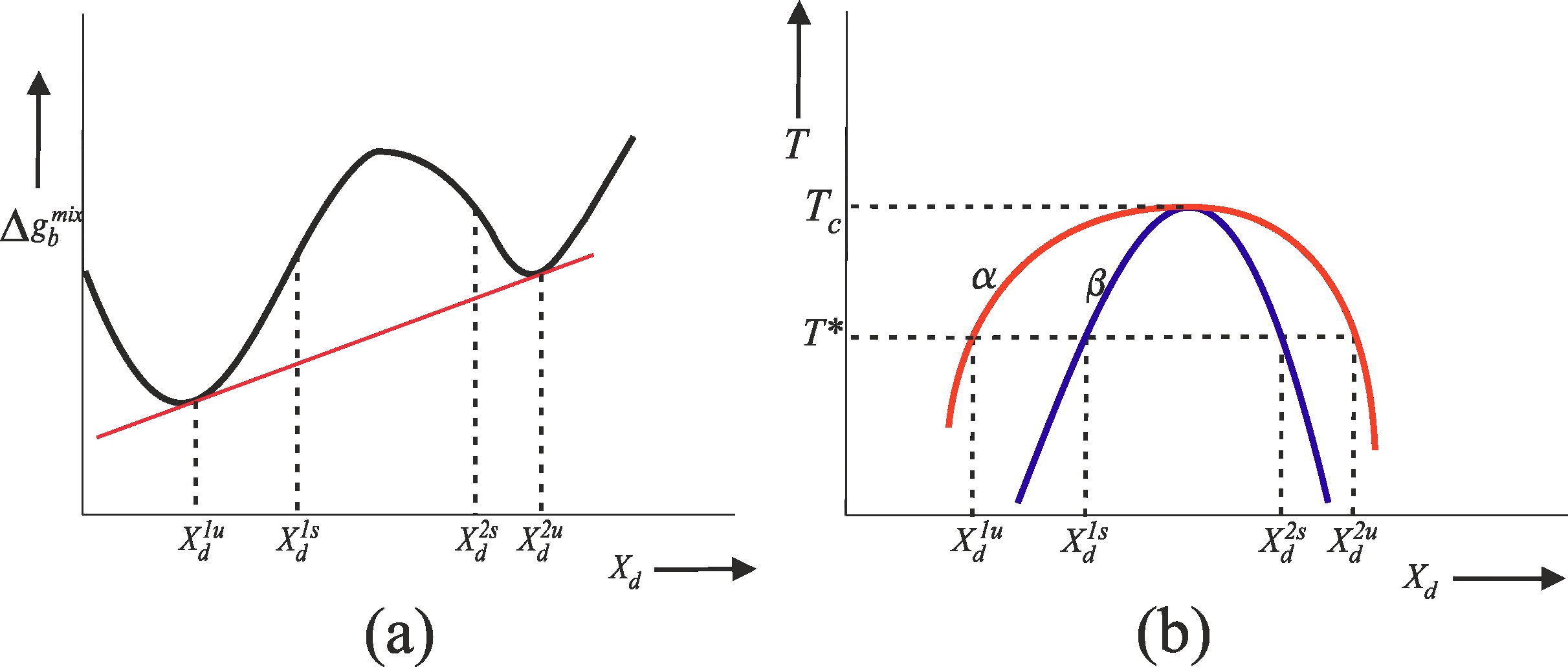
Figure 2: (a) Plot of the bulk free energy of mixing $\Delta g_{b}^{mix}$ as a function of a drug molar fraction $X_{d}$. The spinodal points $X_{d}^{1s}$, $X_{d}^{2s}$ are the solutions to $d^{2}(\Delta g_{b}^{mix})/dX_{d}^{2}=0$. In the spinodal region $(X_{d}^{1s},X_{d}^{2s})$, we have $d^{2}(\Delta g_{b}^{mix})/dX_{d}^{2}<0$ and $D_{\mbox{\scriptsize eff}}(X_{d})<0$. (b) Phase diagram for the binary mixture. Here $\alpha$ is the coexistence curve, $\beta$ is the spinodal curve, $T^{*}$ is the temperature for the free energy density diagram in (a), and $T_{c}$ is the critical temperature above which the dispersion is homogeneous.

In Figure 2 (a), we plot a free energy of mixing diagram $\Delta g_{b}^{mix}$ as a function of drug molar fraction $X_{d}$. In this diagram, the points $X_{d}^{1s}$, $X_{d}^{2s}$ are the solutions to

$$\frac{d^{2}\left(\Delta g_{b}^{mix}\right)}{dX_{d}^{2}}=0,$$

and are referred to as the spinodal points. The region $(X_{d}^{1s},X_{d}^{2s})$ is referred as the spinodal region, and for points $X_{d}$ in this region, we have

$$\frac{d^{2}\left(\Delta g_{b}^{mix}\right)}{dX_{d}^{2}}<0.$$

Compositions $X_{d}$ in the spinodal region are unstable, and will split into two phases characterized by the compositions $X_{d}^{1u}$ and $X_{d}^{2u}$ as shown in Figure 2 (a); see [37] for more details. The points $X_{d}^{1u}$, $X_{d}^{2u}$ are referred to as the binodal points, and are defined by the common tangent construction shown in Figure 2 (a). The binodal and spinodal points define the coexistence and spinodal curves, respectively, and these are plotted in the phase diagram shown in Figure 2 (b).

Using equation (34), we obtain

$$\frac{d^{2}(\Delta g_{b}^{mix})}{dX_{d}^{2}}=RT\frac{q(X_{d})}{(1-(1-1/m)X_{d})^{3}X_{d}(1-X_{d})}$$ (35)

where

$$q(X_{d})=AX_{d}^{2}+BX_{d}+1$$ (36)

and where

$$A=\frac{1}{m^{3}}-\frac{1}{m^{2}}-(1-2\chi_{dp})\frac{1}{m}+1,\hskip 14.22636ptB=\frac{1}{m^{2}}+(1-2\chi_{dp})\frac{1}{m}-2.$$ (37)

Hence there is a spinodal region with $d^{2}(\Delta g_{b}^{mix})/dX_{d}^{2}<0$ if $q(X_{d})<0$ in this region. Inspecting (36), we see that $q(X_{d})$ can be negative if $q(X_{d})=0$ has real roots, that is, if

$$B^{2}-4A>0,$$

and using (37), this leads to

$$(2\chi_{dp}-(1+1/m))^{2}-4/m>0$$

which holds true if

$$\chi_{dp}>\frac{1}{2}\left(1+\frac{1}{\sqrt{m}}\right)^{2}=\frac{1}{2}\left(1+\sqrt{V_{d}/V_{p}}\right)^{2}.$$

Hence, we have a spinodal interval if

$$\chi_{dp}>\chi_{dp}^{c}(m)$$ (38)

where

$$\chi_{dp}^{c}(m)\equiv\frac{1}{2}\left(1+\frac{1}{\sqrt{m}}\right)^{2},$$ (39)

and where $\chi_{dp}^{c}(m)$ is a critical value for the Flory-Huggins parameter. If (38) holds true, then there is a spinodal interval $(X_{d}^{1s},X_{d}^{1s})\subset[0,1]$ where

$$X_{d}^{1s}=\frac{-B-\sqrt{B^{2}-4A}}{2A},\hskip 8.5359ptX_{d}^{2s}=\frac{-B+\sqrt{B^{2}-4A}}{2A},$$ (40)

and where $A$, $B$ are given in (37).

The diffusion coefficient and spinodal decomposition

Using (24) and (35), elementary calculations show that

$$D_{\mbox{\scriptsize eff}}(X_{d})=M^{\dagger}(X_{d})\frac{d^{2}(\Delta g_{b}^{mix})}{dX_{d}^{2}}$$ (41)

where

$$M^{\dagger}(X_{d})=M_{d}X_{d}(1-X_{d})$$

with $M_{d}=D_{d}/RT$, and where $M^{\dagger}(X_{d})$ is a concentration-dependent drug mobility; see, for example, equation (3.6) of the paper [40]. Hence, for $0<X_{d}<1$, it is clear from (41) that $d^{2}(\Delta g_{b}^{mix})/dX_{d}^{2}<0$ implies that

$$D_{\mbox{\scriptsize eff}}(X_{d})<0.$$ (42)

Hence, an equivalent criterion for spinodal decomposition to occur is that there exist a region in $0\leq X_{d}\leq 1$ where $D_{\mbox{\scriptsize eff}}(X_{d})<0$, that is, that there exist a region where drug diffusion is against the concentration gradient (uphill diffusion).

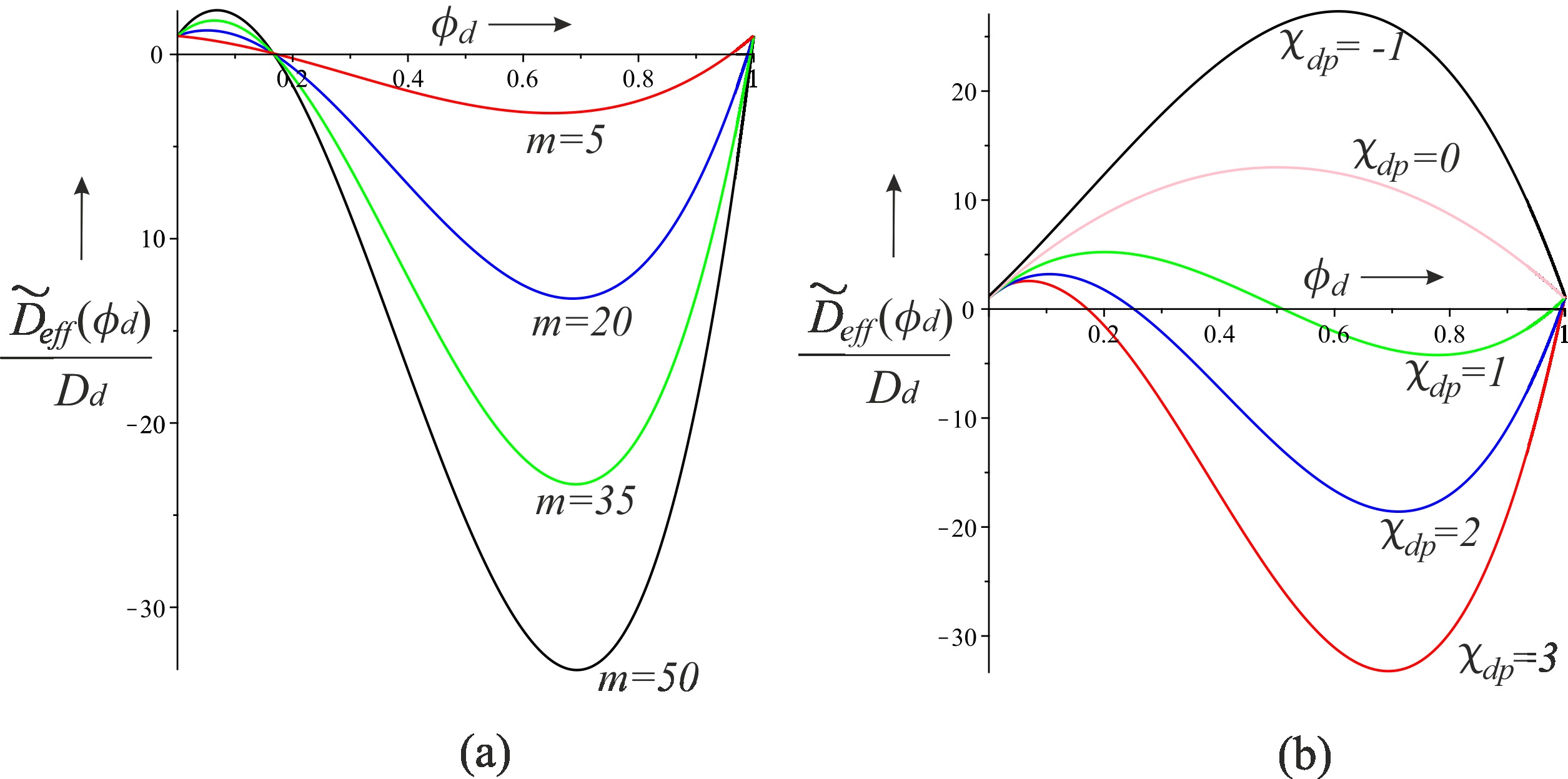
Figure 3: Plots of the scaled effective diffusion coefficient for the drug in the polymer dispersion as a function of the drug volume fraction. Here positive values of the diffusion coefficient correspond to standard drug diffusion down the concentration gradient, while negative values correspond to phase separation of the drug and the polymer, with larger negative values (in absolute terms) corresponding to more rapid phase separation. We have plotted the scaled drug diffusion coefficient for (a) the Flory-Huggins interaction parameter $\chi_{dp}=3$ and various values of the polymer chain length $m$, and, (b) polymer chain length $m=50$ and various values of the Flory-Huggins interaction parameter $\chi_{dp}$. See the main body of the text for further discussion.

3 Qualitative results and discussion

Although the model we have derived in the current study is quite general, and is not tied to any specific statistical model for a solid dispersion, the detailed results we shall present in this section are for the Flory-Huggins case.

3.1 The effective diffusion coefficient for the drug in the dispersion

From (25), the scaled effective diffusion coefficient for the drug in the dispersion is given by

$$\frac{\tilde{D}_{\mbox{\scriptsize eff}}(\phi_{d})}{D_{d}}=(1+(m-1)\phi_{d})\left(1+\left(\frac{1}{m}-1\right)\phi_{d}-2\chi_{dp}\phi_{d}(1-\phi_{d})\right)$$ (43)

where we recall that $D_{d}$ is the temperature-dependent self-diffusion coefficient for the drug. Equation (43) is of particular value since it yields information on how the mobility of the drug in the dispersion depends on the polymer chain length, the dispersion composition, and the character of the drug-polymer interaction.

In Figure 3 (a), we have plotted (43) for the Flory-Huggins interaction parameter $\chi_{dp}=3$ (which is in the unstable regime) and various values of the polymer chain length $m$. It should be emphasized that positive values for $\tilde{D}_{\mbox{\scriptsize eff}}$ correspond to standard drug diffusion down the concentration gradient, while negative values correspond to unstable regimes where phase separation of the drug and polymer can occur. In Figure 3 (a), it is clear that if the drug loading $\phi_{d}$ is sufficiently low, then $\tilde{D}_{\mbox{\scriptsize eff}}>0$ and the solid dispersion is stable. However, for larger (and more realistic) drug loadings, $\tilde{D}_{\mbox{\scriptsize eff}}<0$, and the system is unstable. It is interesting to note that the system becomes more unstable as the length of the polymer chains increase.

It is also clear from the curves in Figure 3 (a) that the relationship between the initial drug loading in the dispersion and the initial rate of phase separation is not altogether obvious. It is not necessarily the case that increasing drug loading corresponds to increasing initial dispersion instability. Rather, there is in fact a well defined worst choice for the initial drug loading from the point of view of stability in the initial stages. This worst choice corresponds to the minima of the curves displayed in Figure 3 (a), since these minima correspond to the fastest rates of phase separation. For $m\gg 1$, the minimum of $\tilde{D}_{\mbox{\scriptsize eff}}(\phi_{d})$ occurs at

$$\phi_{d}^{min}\approx\frac{1+2\chi_{dp}+\sqrt{(1+2\chi_{dp})^{2}-6\chi_{dp}}}{6\chi_{dp}}.$$ (44)

These theoretical results predict that choosing initial drug loadings $\phi_{d}$ above or below $\phi_{d}^{min}$ should lead to improved dispersion stability in the initial stages. For $m,\chi_{dp}\gg 1$, we have $\phi_{d}^{min}\approx 0.67$.

In Figure 3 (b), we plot (43) for the fixed polymer length $m=50$, and various values of the Flory-Huggins interaction parameter $\chi_{dp}$. For $m=50$, the critical value for $\chi_{dp}$ is given by $\chi_{dp}^{c}\approx 0.5707$ (see equation (39)). Recall that for $\chi_{dp}<\chi_{dp}^{c}$, the system is stable for all drug loadings $\phi_{d}$, and that for $\chi_{dp}>\chi_{dp}^{c}$, there is a regime of unstable drug loadings. This is borne out by the curves displayed in Figure 3 (b). These curves predict that the system becomes more unstable with increasing values of $\chi_{dp}$, and this is as expected given the dependence of $\chi_{dp}$ on the interaction energies - see equation (4).

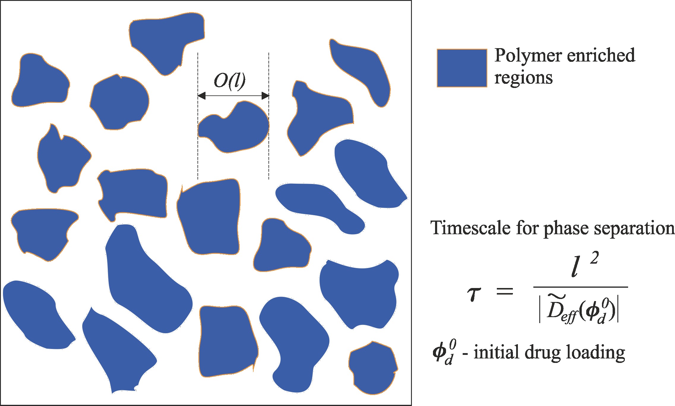
Figure 4: Schematic of a phase separating solid dispersion where polymer-rich regions with characteristic lengthscale $l$ have formed. A formula for the timescale of evolution of such a dispersion is given in the main body of the text; see equation (45).

3.2 Timescale for phase separation in a solid dispersion

In Figure 4, we give a schematic of a phase separating solid dispersion where polymer-rich regions have formed. The characteristic lengthscale of these regions is denoted by $l$. In order for such regions to form, the drug must have diffused away over a lengthscale of order $l$, and the timescale over which this diffusion occurs is estimated by (see (25))

$$\tau=\frac{l^{2}}{|\tilde{D}_{\mbox{\scriptsize eff}}(\phi_{d}^{0})|}=\frac{l^{2}}{D_{d}(T)}\frac{1}{|(1+(m-1)\phi_{d}^{0})[1+(1/m-1)\phi_{d}^{0}-2\chi_{dp}(T)\phi_{d}^{0}(1-\phi_{d}^{0})]|}$$ (45)

where $\phi_{d}^{0}$ is the initial uniform volume fraction of the drug in the dispersion, and $T$ is a representative storage temperature. It should be emphasized that this formula is just an estimate since, in reality, the drug volume fraction evolves in space and time. Hence, (45) should only be used as a rough rule of thumb. In Section 4, we evaluate this formula by comparing it with detailed numerical results, and satisfactory agreement is generally found.

Equation (45) may, in appropriate circumstances, be used to estimate the shelf life of a solid dispersion product. To see this, suppose that $l$ denotes the largest acceptable size for polymer-rich domains (or drug-rich domains) in the product. Then, since $\tau$ estimates the timescale for these regions to form, it also estimates the timescale for the shelf life of the product. However, care should be taken when using (45) since, apart from the fact that is based on a fixed value of $\phi_{d}$, it also incorporates a number of significant assumptions - for example, it assumes that the dispersion is perfectly dry, and that Flory-Huggins theory is an appropriate statistical model for the system.

3.3 Criteria for a stable solid dispersion

Although the drug loading in real solid dispersions is typically high and in the unstable regime, it is nevertheless worthwhile specifying conditions under which the stability of the dispersion is guaranteed. The results we display here are based on the discussion given in Section 2.4. For $\chi_{dp}<\chi_{dp}^{c}$ where $\chi_{dp}^{c}=\frac{1}{2}\left(1+1/\sqrt{m}\right)^{2}$, the system is stable irrespective of the choice of the uniform initial drug load $\phi_{d}^{0}$. For $\chi_{dp}>\chi_{dp}^{c}$, the dispersion is unstable if the initial drug loading $\phi_{d}^{0}$ is chosen in the interval $(\phi_{d}^{-},\phi_{d}^{+})$, but stable if chosen in either of the intervals $(0,\phi_{d}^{-})$ or $(\phi_{d}^{+},1)$, where

$$\phi_{d}^{\pm}=\frac{1}{2}\left\{1+\frac{1}{2\chi_{dp}}\left(1-\frac{1}{m}\right)\pm\sqrt{\left[1+\frac{1}{2\chi_{dp}}\left(1-\frac{1}{m}\right)\right]^{2}-\frac{2}{\chi_{dp}}}\right\}.$$

These results are based on the bulk free energy only, and do not take account of interfacial energy. However, the interfacial energy can be readily incorporated into the analysis, and this is discussed in Appendix A.

4 Numerical results and discussion

4.1 The numerical method

For the purposes of numerical calculations, we take the integration domain to be the square region $\Omega=\{(x,y)|\hskip 2.84544pt0<x<L,0<y<L\}$ with boundary $\partial\Omega$. The governing equation to be solved is defined by the equations (26), (27) and (28). The boundary conditions are given by

$$\nabla\psi\cdot{\bf n}=0\hskip 8.5359pt\mbox{ and }\hskip 8.5359pt\nabla X_{d}\cdot{\bf n}=0\hskip 8.5359pt\mbox{ on }\hskip 2.84544pt\partial\Omega,$$ (46)

and the initial condition takes the form (31). The boundary conditions (46) are equivalent to those given in (30). The governing equation was numerically integrated using the finite element package COMSOL Multiphysics. A mesh sensitivity analysis was performed to investigate the influence of the size of the mesh on the results. The solution was assumed to be mesh independent when there was less than 1% difference in the mole fraction of drug between successive refinements. The final mesh used in the simulations was triangular and consisted of 7553 vertices and 14796 triangles. The numerical solutions all conserved the total mass of drug in the system to within 1%.

4.2 Parameter values

We consider parameter values that are appropriate for a solid dispersion consisting of the drug Felodipine (FD) and the polymeric excipient HPMCAS. Felodipine is a calcium channel blocker that is commonly used to treat blood pressure. For this system, the Flory-Huggins interaction parameter is given as a function of temperature by (see [16])

$$\chi_{dp}(T)=-18.767+\frac{7830.4}{T}.$$ (47)

Using data taken from [16], the molar volume for FD is $V_{d}=300.19$ cm³/mol and the molar volume of HPMCAS is $V_{p}=14007.78$ cm³/mol, so that

$$m=\frac{V_{p}}{V_{d}}=\frac{14007.78}{300.19}\approx 46.6630.$$

From (39), the critical value for the interaction parameter below which phase separation cannot occur is given by

$$\chi_{dp}^{c}(m)=\frac{1}{2}\left(1+\frac{1}{\sqrt{m}}\right)^{2}=0.6571.$$

The self-diffusion coefficient for Felodipine was estimated in [41] (Chapter 4, page 133) to be

$$D_{d}(T)=\exp(-A_{1})\exp\left(-\frac{A_{2}}{T}\exp\left(\frac{A_{3}}{T}\right)\right)\hskip 5.69046pt\mbox{m}^{2}\mbox{s}^{-1}$$ (48)

where $A_{1}=18.03$, $A_{2}=445.84$ K, $A_{3}=874.81$ K. Some illustrative values for the diffusion coefficients and the Flory-Huggins interaction parameter are displayed in Table 1.

For the numerical simulations displayed in the current study, we take the size of the square domain to be given by $L=2$ mm. The thickness of the interfacial regions is dictated by the parameter $\delta_{d}$, and here we chose the value $\delta_{d}=L/50=4\times 10^{-5}$ m. We illustrate how the initial conditions were specified by considering a particular case. We consider the case where the initial weight fraction of drug is 80%. This means that the initial weight of FD divided by the weight of FD plus the weight of HPMCAS is 0.8. This corresponds to an initial molar drug fraction of $X_{d}=0.9947$. More precisely, we choose the initial molar fraction of drug to be a small random perturbation about this level given by

$$X_{d}(x,y,t=0)=0.9947(1+rnd(x,y))$$

where $rnd(x,y)$ is a normally distributed random function with a mean value of zero and a standard deviation of $10^{-5}$. The standard deviation for all of the initial conditions was taken to be $10^{-5}$, with one exception - the numerical results displayed in Figure 6 took the larger value $0.007$ to simulate a coarse initial mixture in a hot melt extruder.

In Figure 5, we plot the phase diagram for the Felodipine/HPMCAS system. All that is required to calculate the phase diagram here is a knowledge of the Flory-Huggins interaction parameter, and this has been given in (47). The spinodal curve $T_{s}(\phi_{d})$ is obtained by setting $\tilde{D}_{\mbox{\scriptsize eff}}(\phi_{d})=0$ in (43) to obtain

$$1+\left(\frac{1}{m}-1\right)\phi_{d}-2\chi_{dp}\phi_{d}(1-\phi_{d})=0,$$ (49)

where $\chi_{dp}$ is given by (5). Solving (49) for $T$ gives the spinodal curve

$$T_{s}(\phi_{d})=\frac{2\beta\phi_{d}(1-\phi_{d})}{1+\left(\frac{1}{m}-1\right)\phi_{d}-2\alpha\phi_{d}(1-\phi_{d})}$$

where $\alpha=-18.767$, $\beta=7830.4$, $m=46.6630$ for the Felodipine/HPMCAS system. The binodal curve was estimated numerically. The calculation involved simultaneously solving the pair of equations $\mu_{d}^{b}(X_{d}^{1u})=\mu_{d}^{b}(X_{d}^{2u})$ and $\mu_{p}^{b}(X_{d}^{1u})=\mu_{p}^{b}(X_{d}^{2u})$ for the binodal points $X_{d}^{1u}$, $X_{d}^{2u}$ with $X_{d}^{1u}<X_{d}^{2u}$. This was implemented using the the fsolve command in MAPLE.

$T$ (${}^{\mbox{o}}$C)	$\chi_{dp}(T)$	$D_{d}(T)$ (m2s-1)	$D_{\mbox{\scriptsize eff}}(X_{a})$ (m2s-1)
$40$	6.2383	$1.1661\times 10^{-18}$	$8.8605\times 10^{-17}$
$50$	5.4645	$1.5494\times 10^{-17}$	$1.0113\times 10^{-15}$
$60$	4.7371	$1.3787\times 10^{-16}$	$7.6107\times 10^{-15}$
$75$	3.7245	$2.0297\times 10^{-15}$	$8.3587\times 10^{-14}$
$90$	2.7954	$1.7356\times 10^{-14}$	$4.9151\times 10^{-13}$
$100$	2.2176	$5.7436\times 10^{-14}$	$1.1670\times 10^{-12}$
$110$	1.6699	$1.6336\times 10^{-13}$	$2.0806\times 10^{-12}$
$120$	1.1501	$4.0902\times 10^{-13}$	$2.2657\times 10^{-12}$

Table 1: Illustrative values for some of the parameters of the FD/HPMCAS system at various temperatures. Here the initial weight fraction of drug is 70%, which corresponds to an initial drug molar fraction $X_{d}\approx 0.9909$.

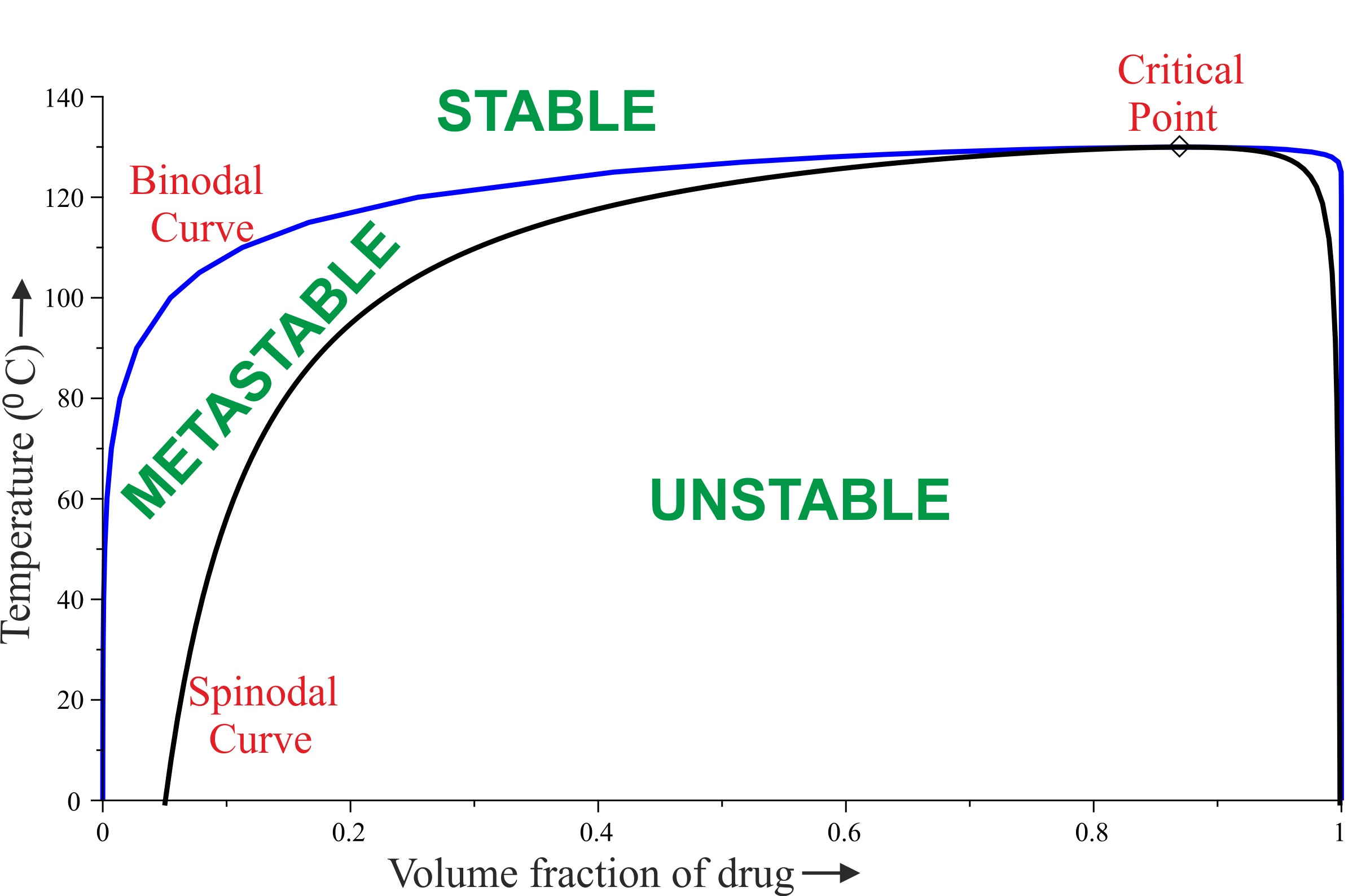
Figure 5: The phase diagram for the Felodipine/HPMCAS system.

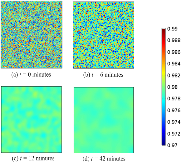
Figure 6: Numerical simulation of the behaviour of a solid dispersion in a hot melt extruder. The simulations here are for a FD/HPMCAS solid dispersion and were obtained by numerically integrating the initial boudary value problem defined in Section 4.1. The colours correspond to different mole fractions of the drug as defined by the colour bar. The weight fraction of drug here is 50%, and the other parameter values can be found in Section 4.2 and Section 4.3. These simulations represent a succesful extrusion where an initially coarse mixture is heated and then cooled to form a well-mixed dispersion.

4.3 Numerical results

The first numerical calculations we display simulate the hot melt mixing process for a Felodipine/HPMCAS system. To implement this, we used a time dependent temperature profile that treats the case where the mixture begins at 25${}^{\mbox{o}}$C and rises in temperature at a rate of 10${}^{\mbox{o}}$C per minute until it reaches 145${}^{\mbox{o}}$C. We then assumed for simplicity that the melt cooled linearly back down to 25${}^{\mbox{o}}$C over a period of 30 minutes. The results of the calculation are shown in Figure 6. We see in Figure 6 (a) that the initial drug/polymer mixture is quite coarse (badly mixed). As the temperature rises, we see from Figure 6 (b) that the mixture becomes increasingly homogenous. By the time the mixture has achieved its maximum temperature, Figure 6 (c), it is quite well-mixed. Figure 6 (d) shows that the amount of phase separation that occurs during the cooling process is insignificant. Hence, the numerical results shown here predict a successful hot melt extrusion process for the manufacture of a solid dispersion. We note that different heating and cooling regimes are easily simulated using the model.

Figure 7: Numerical solutions superimposed on a phase diagram for the Felodipine/HPMCAS system. The numerical solutions shown here are all for a time of six months. The parameter values used can be found in Section 4.2. The dark blue regions are polymer-enriched and the dark red regions are drug-enriched. The green panels correspond to cases where phase separation is not significant.

In Figure 7, we superimpose numerical solutions on a phase diagram for the Felodipine/HPMCAS system. Each of these solutions corresponds to an evolution time of 6 months, with the dispersion mixture beginning from an initially approximate uniform state. We see that there is no significant phase separation for the 30${}^{\mbox{o}}$C degree cases, and for the cases in the metastable and stable regions. This predicts that Felodipine/HPMCAS systems should not suffer considerable phase separation under normal storage temperatures. However, we should caution that we are modelling the case of zero relative humidity here. For the cases that do exhibit significant phase separation, we note a coarser separation morphology for higher temperatures. In these figures, dark red corresponds to drug-enriched domains (relative to the initial concentration) while dark blue correspond to polymer-enriched domains. We also note the occurrence of polymer droplets and strings - we return to this issue below.

Further numerical simulations are displayed in Figures 8, 9, 10, 11, and these correspond to weight fractions of drug of 80%, 60%, 40% and 20%, respectively. Recall that decreasing weight fractions of drug correspond to increasing weight fractions of polymer since the system is binary. In a given figure, each column corresponds to a given temperature as labelled, and reading a column from top to bottom corresponds to increasing time for the dispersion for the given temperature. We have chosen here not to use the same times for the different temperatures since the rate at which a dispersion evolves depends on temperature.

$T=60^{\circ}C$	$T=90^{\circ}C$	$T=120^{\circ}C$
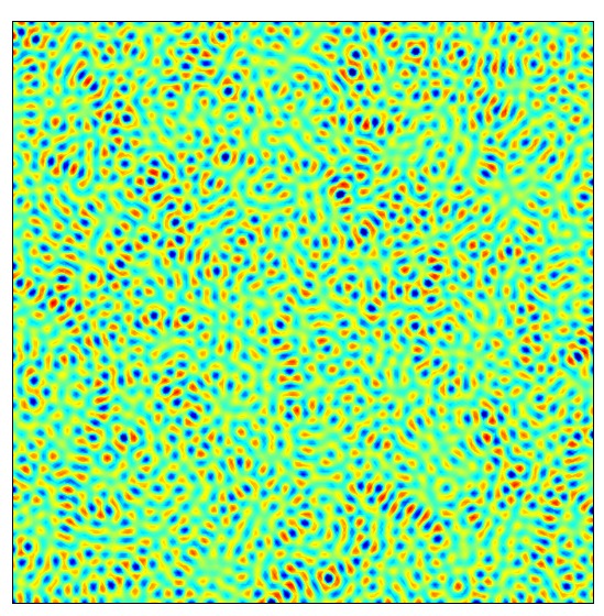
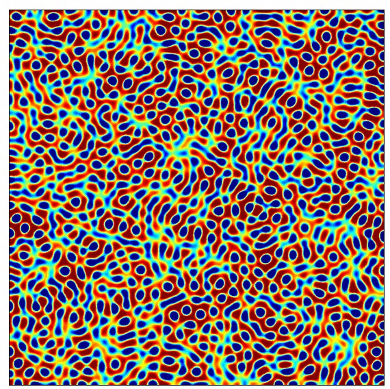
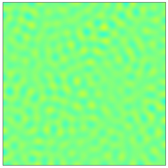
1 day	1 hour	0.5 hours
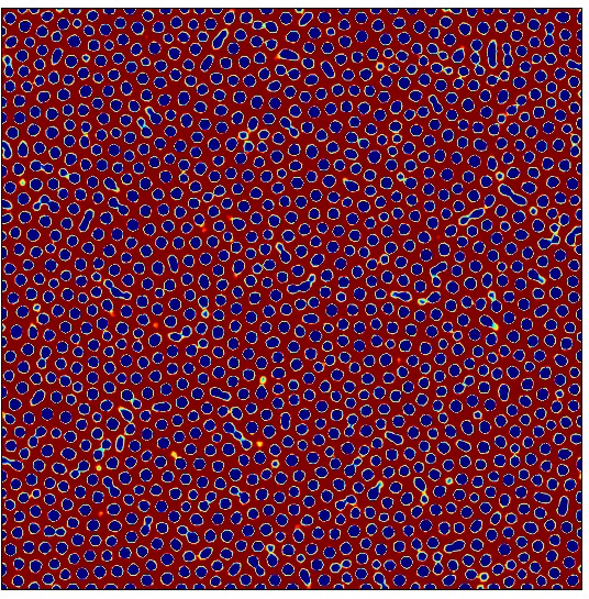
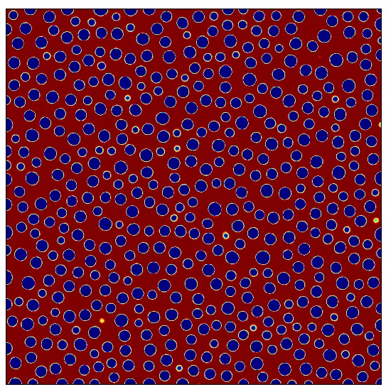
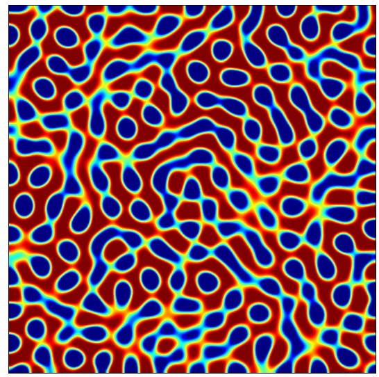
2 days	3 hours	1 hour
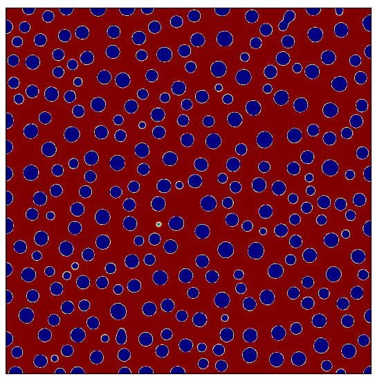
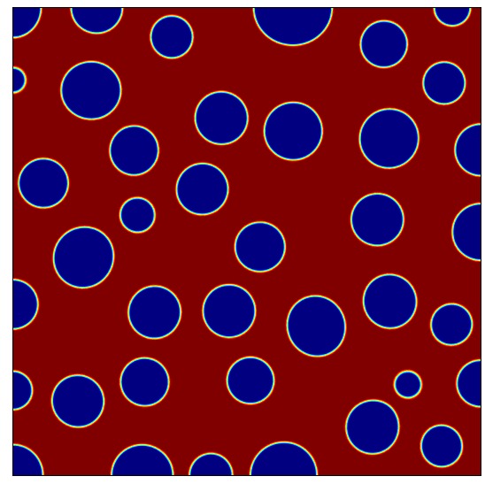
1 week	4 hours	1 day
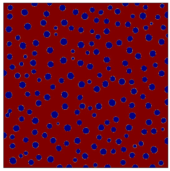
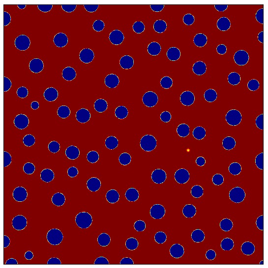
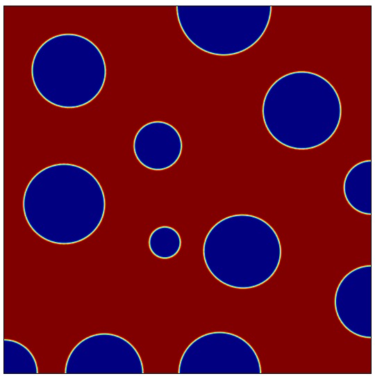
1 month	1 day	1 week
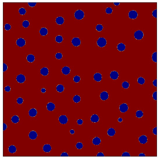
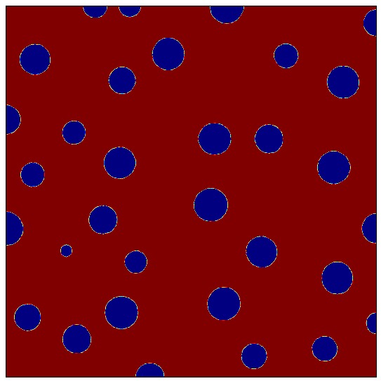
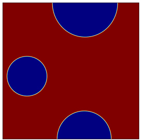
6 months	1 week	2 months

Figure 8: Simulations of a FD/HPMCAS solid dispersion obtained by numerically integrating the initial boudary value problem defined in Section 4.1. The colours correspond to different mole fractions of the drug as defined by the colour bar. The weight fraction of drug here is 80%, and the other parameter values can be found in Section 4.2. In the above frame of figures, each column corresponds to a different temperature, and reading a column from top to bottom corresponds to increasing time for the dispersion for the given temperature.

$T=60^{\circ}C$	$T=90^{\circ}C$	$T=120^{\circ}C$
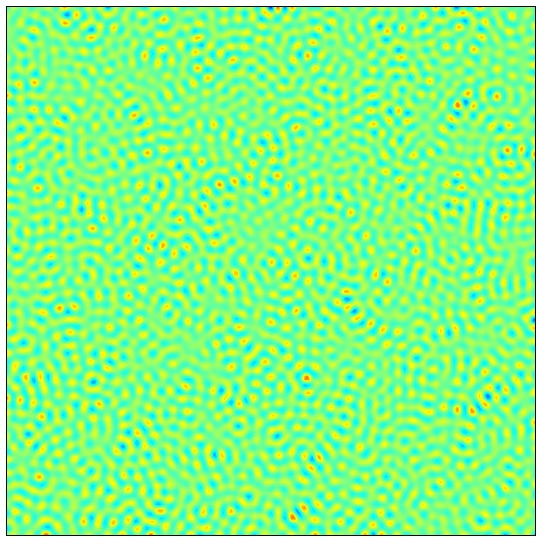
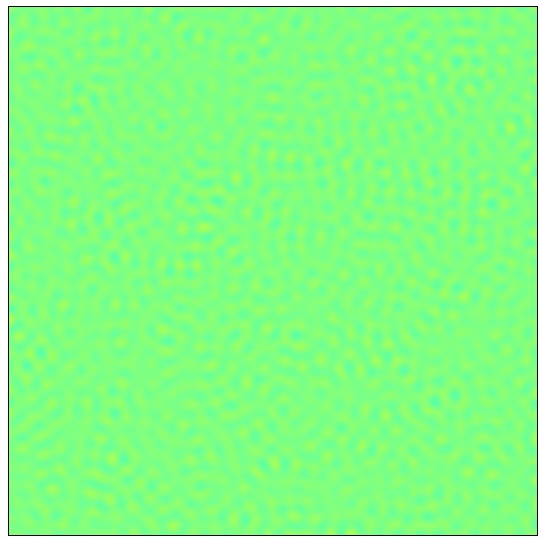
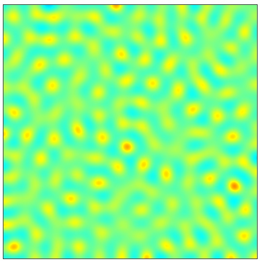
1 day	0.5 hours	1.5 hours
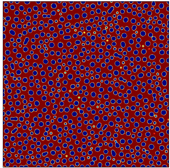
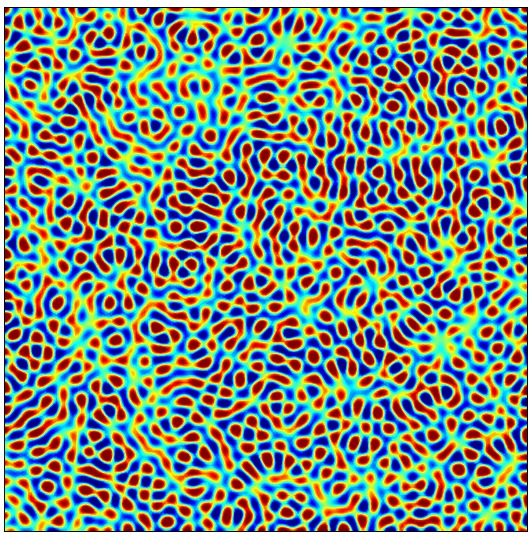
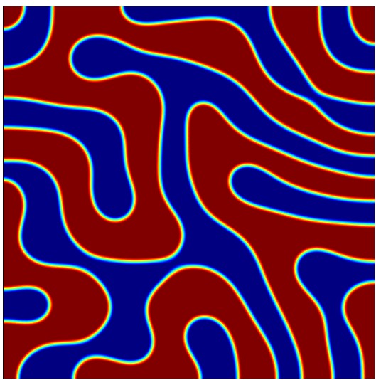
1 week	1 hour	1 day
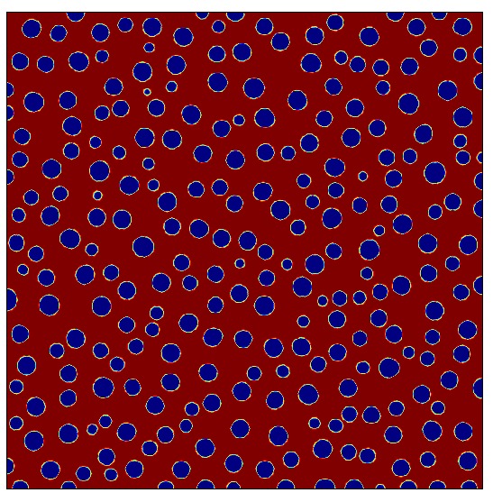
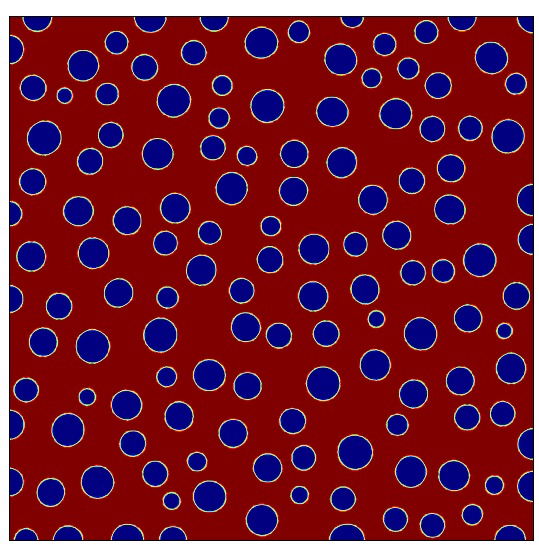
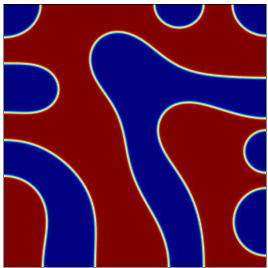
1 month	1 day	1 week
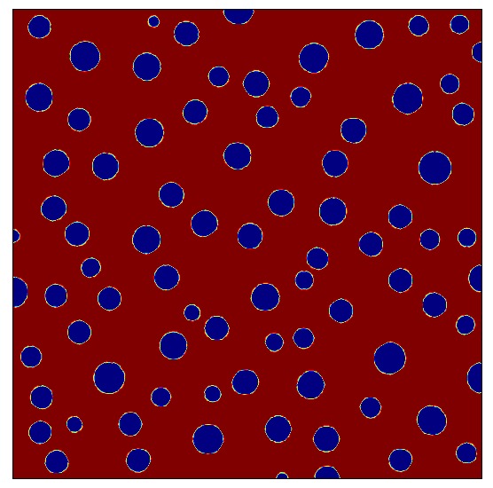
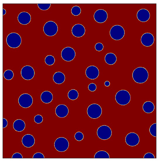
6 months	1 week	1 month
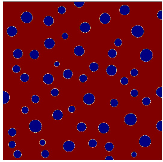
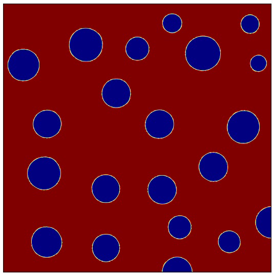
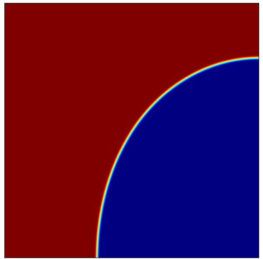
1 year	1 month	9 months

Figure 9: See the caption for Figure 8. The weight fraction of drug here is 60%.

$T=60^{\circ}C$	$T=90^{\circ}$ C	$T=110^{\circ}C$
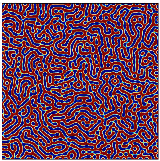
1 week	3 hours	3 hours
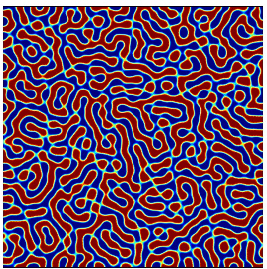
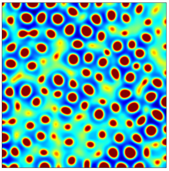
2 weeks	6 hours	6 hours
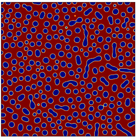
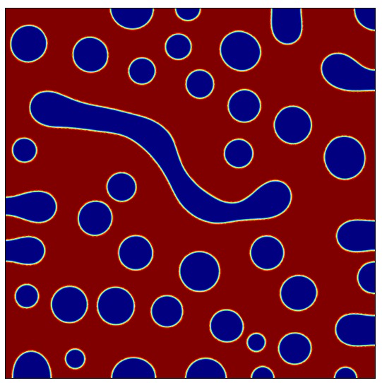
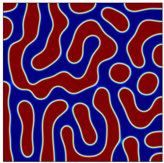
1 month	1 week	1 day
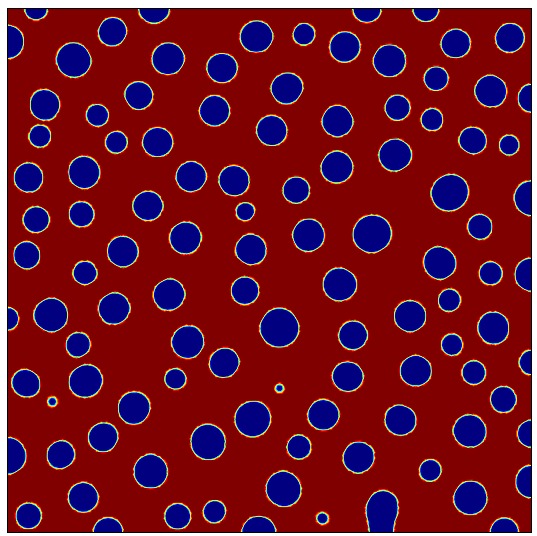
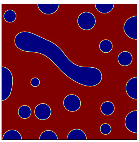
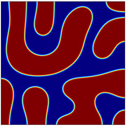
6 months	1 month	1 week
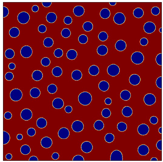
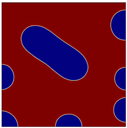
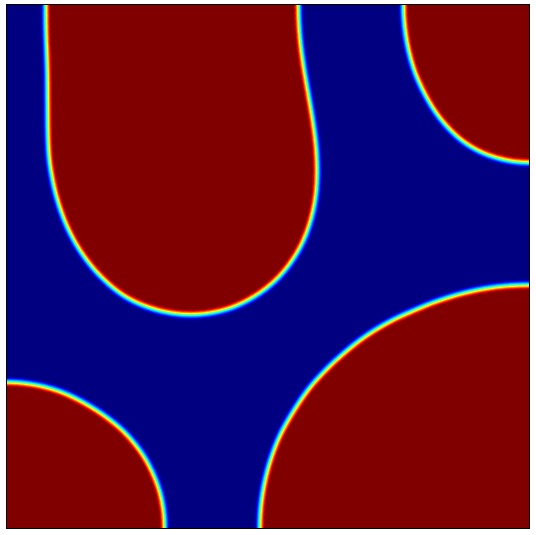
1 year	6 months	4 months

Figure 10: See the caption for Figure 8. The weight fraction of drug here is 40%.

$T=60^{\circ}C$	$T=75^{\circ}$ C	$T=90^{\circ}C$
1 month	2 weeks	2 weeks
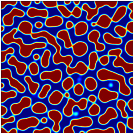
2 months	23 days	23 days
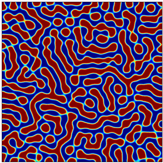
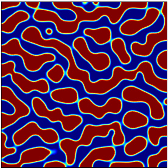
4 months	1 month	1 month
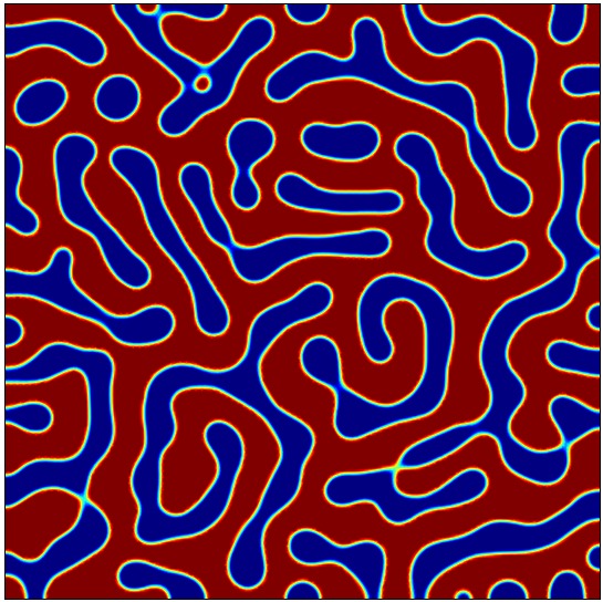
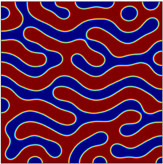
9 months	2 months	2 months
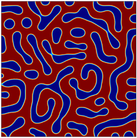
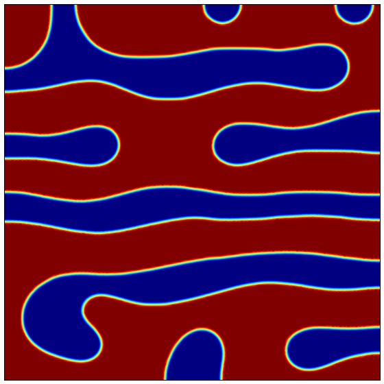
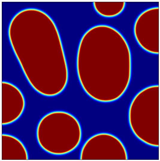
1 year	9 months	9 months

Figure 11: See the caption for Figure 8. The weight fraction of drug here is 20%.

We now highlight some notable features of these numerical simulations.

• Two phases eventually emerge. The numerical results show that the systems eventually evolve into two distinct phases, characterized by deep blue domains (polymer-rich) and deep red domains (drug-rich).

• Ostwald ripening/coarsening. Another notable feature in many of the numerical illustrations is the formation of polymer droplets (blue discs) in the dispersion, followed by a subsequent growth in their size; see, for example, the third column in Figure 8. This is a well-known and common phenomenon in multicomponent solid systems, and is often referred to as Ostwald ripening or coarsening [42]. We also note the general trend that dispersions at higher temperature tend to be coarser.

• Phase inversion. The system exhibits the phase inversion phenomenon [31] as the polymer content increases. To see this, consider the panels in Figure 8. These correspond to the case where the polymer content is low (20% by weight), and we see the emergence of polymer droplets in drug-dominated domains. Compare these with the panels in the third column of Figure 11. These correspond to the case where where the polymer content is high (80% by weight), and we see the emergence of drug droplets in polymer-rich domains, the reverse of the low polymer content case.

• Polymer strings and droplet-to-string transitions. We note the formation of polymer strings in some of the panels; see the first and second columns of Figure 11 for examples. The central column in Figure 11 is of particular interest since the behaviour exhibited here is an example of a droplet-to-string transition [43]. In this droplet-to-string transition, drug droplets coalesce to form long drug-rich strings. In the panel for 23 days, we observe that drug droplets are in the process of chaining [43]. Another droplet-to-string transition is shown in Figure 12.

• The formula (45) for the timescale for phase separation. The detailed numerical results here enable us to test the utility of our simple formula (45) for the timescale for phase separation. Consider, for example, the panel corresponding to 1 day in the third column of Figure 8. Here we see that polymer droplets with characteristic lengthscale of $l\approx 0.3$ mm have formed. Our formula (45) predicts that such droplets should form over a timescale dictated by

  $$\tau\approx\frac{(0.3)^{2}\mbox{mm}^{2}}{|\tilde{D}_{\mbox{\scriptsize eff}}(\phi_{d}=0.8006)|}\approx 11\hskip 5.69046pt\mbox{hours}$$

  which is consistent with the time $t=1$ day for the panel since 1 day $\approx 2\tau$. It should be emphasized that $\tau$ does not predict the time for the droplets to form, but rather estimates the timescale over which such droplets form.

5 Conclusions

Solid dispersions have been the subject of intensive research in recent years because of their potential to improve the solubility of drugs, and numerous excellent studies have been published. However, detailed theoretical studies considering the non-equilibrium behaviour of solid dispersions are lacking. Hence, in this study we have developed a general diffusion model for a dissolving solid dispersion. We then considered the particular case of a binary system modelling a solid dispersion in storage, and developed a formula for the effective diffusion coefficient of the drug. We then specialized further to the case of a Flory-Huggins statistical model. Within the context of this theory, we make the following predictions, some of which should be testable experimentally:

1. A solid dispersion can always be made stable by choosing a sufficiently low drug loading; see Figure 3 (a).

2. For unstable regimes, the relationship between the local drug volume fraction $\phi_{d}$ and the rate of phase separation is not obvious; see Figure 3 (a). There is in fact a well-defined value of $\phi_{d}$ that corresponds to the most rapid rate of phase separation, with the rate decreasing for values of $\phi_{d}$ either side of this value.

3. For unstable regimes, the rate of phase separation increases with increasing polymer chain length $m$; see Figure 3 (a).

4. Dispersions become more unstable with increasing value of the Flory-Huggins interaction parameter $\chi_{dp}$; see Figure 3 (b).

5. Binary drug/polymer systems are capable of exhibiting a rich set of dynamical behaviours. In the numerical simulations performed in the current study, we observed the formation of polymer droplets and strings, the phase inversion phenomenon, Ostwald ripening, and droplet-to-string transitions.

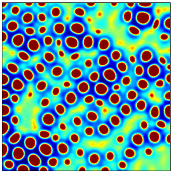
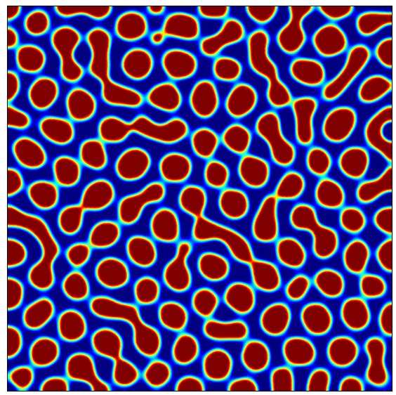
initial time	16 days	20 days
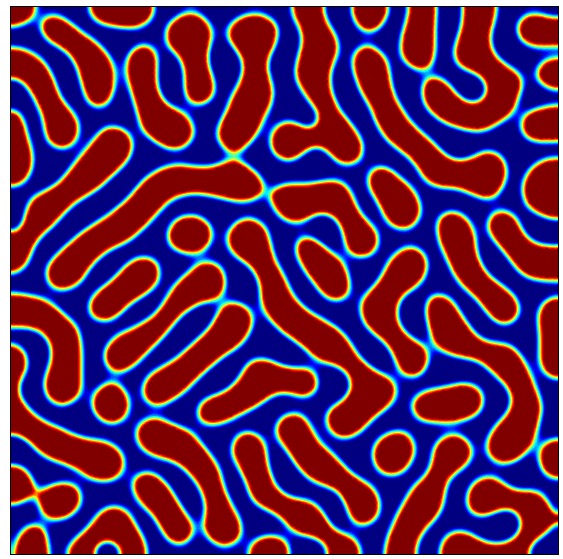
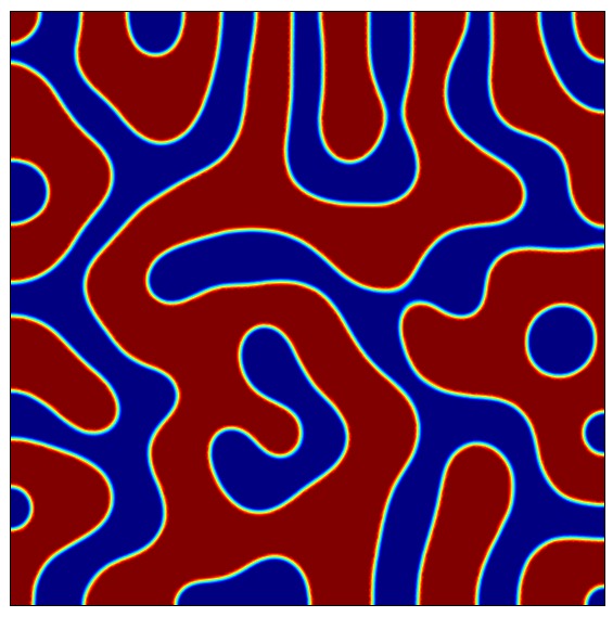
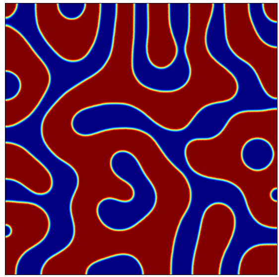
30 days	100 days	4 months
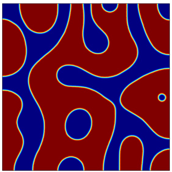
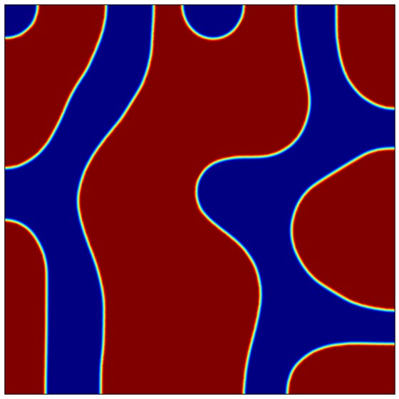
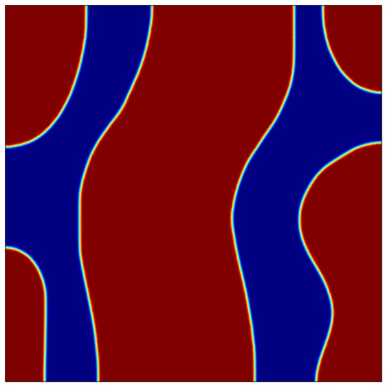
10 months	36 months	80 months

Figure 12: Numerical results illustrating a droplet-to-chain transition. In these panels, the mass fraction of drug is 20% and the temperature is $T=75^{\circ}C$. The panels should be read from left to right, starting at the top row. In the panel for 16 days, we see the formation of drug droplets. The panels for 20 and 30 days show the drug droplets in the process of chaining to form strings. Subesequent panels show the evolution of the drug strings.

The model can be evaluated empirically using microscopy by comparing the theoretical simulations with corresponding images seen in the microscope. Hot-stage polarized light microscopy is one notable possibility - see [44] for a discussion of relevant experimental techniques.

There is ample scope for extending the modelling work presented in the current study. One limitation of the binary model considered here is that it assumes that the polymer is perfectly dry. However, if the dispersions are stored in humid conditions, this is not a good assumption since even small amounts of moisture in the dispersion may significantly affect the mobility of the drug. Another avenue for extending the modelling work developed here is to use statistical models that capture more of the detail of the drug-polymer interaction in the dispersion; see, for example, SAFT models [35]. Viscoelastic effects may also play a significant role in the separation process since the polymer molecules are much larger than the drug molecules in a solid dispersion, giving rise to dynamic asymmetry between the components. Such models are significantly more complex than the model we have considered in the current study; see [45] for some discussion of such models. Another valid critique of the current modelling is that it is incapable of distinguishing between crystalline and amorphous drug. Finally, the we have only considered the storage problem here, and have not addressed the dissolution behaviour at all. The dissolution of solid dispersions is at best partially understood, and there are many open issues that mathematical modelling may help resolve.

It is noteworthy that the current study is the first (that we are aware of) that models in detail the spatiotemporal evolution of solid dispersions. Another novel feature of the current study is the development of an effective diffusion coefficient for the drug in the dispersion, the utility of which has been demonstrated in the results sections. An unusual feature of our modelling is that in equation (11) for the flux of species $i$, we have included the concentration $c_{i}$ of species $i$. This concentration term is frequently omitted in other studies, and a compositionally dependent mobility is assumed instead – see, for example, [32] or [31].

References

- [1] K. T. Savjani, A. K. Gajjar, J. K. Savjani, Drug solubility: importance and enhancement techniques, ISRN Pharmaceutics 2012 (2012) 1–10.
- [2] H. D. Williams, N. L. Trevaskis, S. A. Charman, R. M. Shanker, W. N. Charman, C. W. Pouton, C. J. H. Porter, Strategies to address low drug solubility in discovery and development, Pharmacological Reviews 65 (2013) 315–499.
- [3] S. Kalepua, V. Nekkantib, Insoluble drug delivery strategies: review of recent advances and business prospects, Acta Pharmaceutica Sinica B 5 (5) (2015) 442–453.
- [4] C. Brough, R. O. W. III, Amorphous solid dispersions and nano-crystal technologies for poorly water-soluble drug delivery, International Journal of Pharmaceutics 453 (2013) 157–166.
- [5] Y. Huang, W. Daib, Fundamental aspects of solid dispersion technology for poorly soluble drugs, Acta Pharmaceutica Sinica B 4 (1) (2014) 18–25.
- [6] K. Dhirendra, S. Lewis, N. Udupa, K. Atin, Solid dispersions: a review, Pakistan Journal of Pharmaceutical Sciences 22 (2) (2009) 234–246.
- [7] W. N. Souery, C. J. Bishop, Clinically advancing and promising polymer-based therapeutics, Acta Biomaterialia 67 (2018) 1–20.
- [8] C. G. Garcia, K. L. Kiick, Methods for producing microstructured hydrogels for targeted applications in biology, Acta Biomaterialia 84 (2019) 34–48.
- [9] J. Brouwers, M. E. Brewster, P. Augustijns, Supersaturating drug delivery systems: the answer to solubility-limited oral bioavailability?, Journal of Pharmaceutical Sciences 98 (8) (2009) 2549–2572.
- [10] M. Doi, Introduction to polymer physics, Oxford University Press, Oxford, UK, 1996.
- [11] P. J. Flory, Thermodynamics of high polymer solutions, Journal of Chemical Physics 10 (1942) 51–61.
- [12] M. L. Huggins, Solutions of long chain compounds, Journal of Chemical Physics 9.
- [13] P. C. Hiemenz, T. P. Lodge, Polymer Chemistry, 2nd Edition, CRC Press, Boca Raton, Florida, 2007.
- [14] J. Djuris, I. Nikolakakis, S. Ibric, Z. Djuric, K. Kachrimanis, Preparation of carbamazepine–soluplus solid dispersions by hot-melt extrusion, and prediction of drug–polymer miscibility by thermodynamic model fitting, European Journal of Pharmaceutics and Biopharmaceutics 84 (2013) 228–237.
- [15] Y. Tian, V. Caron, D. S. Jones, A. M. Healy, G. P. Andrews, Using Flory–Huggins phase diagrams as a pre-formulation tool for the production of amorphous solid dispersions: a comparison between hot-melt extrusion and spray drying, Journal of Pharmacy and Pharmacology 66 (2013) 256–274.
- [16] Y. Tian, J. Booth, E. Meehan, D. Jones, S. Li, G. Andrews, Construction of drug-polymer thermodynamic phase diagram using Flory-Huggins interaction theory: identifying the relevance of temperature and drug weight fraction to phase separation within solid dispersions, Molecular Pharmaceutics 10 (2013) 236–248.
- [17] K. Bansal, U. S. Baghel, S. Thakral, Construction and validation of binary phase diagram for amorphous solid dispersion using Flory–Huggins theory, AAPS PharmSciTech 17 (2) (2016) 318–327.
- [18] S. Y. Chan, S. Qia, D. Q. M. Craig, An investigation into the influence of drug–polymer interactions on the miscibility, processability and structure of polyvinylpyrrolidone-based hot melt extrusion formulations, International Journal of Pharmaceutics 496 (2015) 95–106.
- [19] M. A. Altamimi, S. H. Neau, Use of the Flory–Huggins theory to predict the solubility of nifedipine and sulfamethoxazole in the triblock, graft copolymer soluplus, Drug Development and Industrial Pharmacy 42 (3) (2016) 446–455.
- [20] P. Chakravarty, J. W. Lubach, J. Hau, K. Nagapudi, A rational approach towards development of amorphous solid dispersions: Experimental and computational techniques, International Journal of Pharmaceutics 519 (2017) 44–57.
- [21] D. Lin, Y. Huang, A thermal analysis method to predict the complete phase diagram of drug–polymer solid dispersions, International Journal of Pharmaceutics 399 (2010) 109–115.
- [22] K. Wlodarski, W. Sawicki, A. Kozyra, L. Tajber, Physical stability of solid dispersions with respect to thermodynamic solubility of tadalafil in pvp-va, European Journal of Pharmaceutics and Biopharmaceutics 96 (2015) 237–246.
- [23] Y. Zhao, P. Inbar, H. P. Chokshi, A. W. Malick, D. S. Choi, Prediction of the thermal phase diagram of amorphous solid dispersions by Flory–Huggins theory, Journal of Pharmaceutical Sciences 100 (2011) 3196–3207.
- [24] P. J. Marsac, S. L. Shamblin, L. S. Taylor, Theoretical and practical approaches for prediction of drug-polymer miscibility and solubility, Pharmaceutical Research 23 (10) (2006) 2417–2426.
- [25] J. H. Hildebrand, R. L. Scott, The solubility of nonelectrolytes, 3rd Edition, Dover Publications, New York, 1964.
- [26] B. D. Anderson, Predicting solubility/miscibility in amorphous dispersions: it is time to move beyond regular solution theories, Journal of Pharmaceutical Sciences 107 (2018) 24–33.
- [27] E. B. Smith, Basic chemical thermodynamics, sixth Edition, Imperial College Press, London, UK, 2014.
- [28] K. Binder, P. Fratzl, Spinodal decomposition, in: G. Kostorz (Ed.), Phase Transformations in Materials, WILEY-VCH Verlag, Weinheim, 2001, Ch. 6, pp. 411–480.
- [29] D. M. Saylor, C. Kim, D. V. Patwardhan, J. A. Warren, Diffuse-interface theory for structure formation and release behavior in controlled drug release systems, Acta Biomaterialia 3 (2007) 851–864.
- [30] D. M. Saylor, J. E. Guyer, D. Wheeler, J. A. Warren, Predicting microstructure development during casting of drug-eluting coatings, Acta Biomaterialia 7 (2011) 604–613.
- [31] J. Zhu, X. Lu, R. Balieu, N. Kringos, Modelling and numerical simulation of phase separation in polymer modified bitumen by phase-field method, Materials and Design 107 (2016) 322–332.
- [32] J. Zhu, R. Balieu, X. Lu, N. Kringos, Numerical investigation on phase separation in polymer-modified bitumen: effect of thermal condition, Journal of Materials Science 52 (11) (2017) 6525–6541.
- [33] J. W. Cahn, J. E. Hilliard, Free energy of a nonuniform system. i. interfacial free energy, The Journal of Chemical Physics 28 (1958) 258–267.
- [34] N. P. . K. Elder, Phase-field methods in material science and engineering, 1st Edition, John Wiley & Sons, Weinheim, Germany, 2010.
- [35] G. M. Kontogeorgis, G. K. Folas, Thermodynamic models for industrial applications, 1st Edition, John Wiley & Sons, Chichester, West Sussex, UK, 2010.
- [36] J. M. Prausnitz, R. N. Lichtenthaler, E. G. de Azevedo, Molecular thermodynamics of fluid-phase equilibria, 3rd Edition, Prentice Hall, New Jersey, 1999.
- [37] D. A. Porter, K. E. Easterling, M. Sherif, Phase transformations in metals and alloys, 3rd Edition, CRC Press, Boca Raton, Florida, 2009.
- [38] D. L. Elbert, Liquid–liquid two-phase systems for the production of porous hydrogels and hydrogel microspheres for biomedical applications: A tutorial review, Acta Biomaterialia 7 (2011) 31–56.
- [39] P. Atkins, J. de Paula, Elements of physical chemistry, 5th Edition, Oxford University Press, Oxford, England, 2009.
- [40] E. B. Naumana, D. Q. Heb, Nonlinear diffusion and phase separation, Chemical Engineering Science 56 (2001) 1999–2018.
- [41] J. Gerges, Numerical studies of the physical factors responsible for the ability to vitrify/crystallize of model materials of pharmaceutical interest, Ph.D. thesis, Universite de Lille (2015).
- [42] L. Ratke, P. W. Voorhees, Growth and Coarsening: Ostwald Ripening in Material Processing, 1st Edition, Springer, Berlin, 2002.
- [43] K. B. Migler, String formation in sheared polymer blends: Coalescence, breakup, and finite size effects, Physical Review Letters 86 (6) (2001) 1023–1026.
- [44] X. Liu, X. Feng, R. O. W. III, F. Zhang, Characterization of amorphous solid dispersions, Journal of Pharmaceutical Investigation 48 (1) (2018) 19–41.
- [45] H. Tanaka, Viscoelastic phase separation, Journal of Physics:Condensed Matter 12 (15) (2000) 207–264.