Onsager symmetry for systems with broken time-reversal symmetry

Abstract

We provide numerical evidence that the Onsager symmetry remains valid for systems subject to a spatially dependent magnetic field, in spite of the broken time-reversal symmetry. In addition, for the simplest case in which the field strength varies only in one direction, we analytically derive the result. For the generic case, a qualitative explanation is provided.

Introduction.– Onsager reciprocal relations onsager , or the fourth law of thermodynamics, are a cornerstone in nonequilibrium statistical physics. These relations reflect on the macroscopic level the time reversal symmetry of the microscopic dynamics. That is, the equations of motion are invariant under the combined reversal of time $t$ and momenta ${\bm{p}}$: ${\cal T}({\bm{r}},{\bm{p}},t)\equiv({\bm{r}},-{\bm{p}},-t)$ (${\bm{r}}$ being the coordinates). On a macroscopic level, this symmetry has striking consequences on the phenomenological transport coefficients callen ; degrootmazur . Given a system brought out of equilibrium by the thermodynamic forces $\mathcal{F}_{k}$, the coresponding fluxes $J_{k}$ are such that in the linear coupled transport equations $J_{j}=\sum_{k}L_{jk}\mathcal{F}_{k}$ the kinetic coefficient $L_{jk}$ obey the Onsager symmetry $L_{jk}=L_{kj}$. For instance, in thermoelectricity Benenti2017 $\mathcal{F}_{e}$ and $\mathcal{F}_{h}$ are the electrochemical and temperature gradient, $J_{e}$ and $J_{h}$ the charge and heat flow, and the Onsager symmetry implies $L_{he}=L_{eh}$, or equivalently $\Pi=TS$, where $\Pi=L_{he}/L_{ee}$ is the Peltier coefficient and $S=L_{eh}/TL_{ee}$ is the Seebeck coefficient (or thermopower), $T$ being the temperature. That is, as a consequence of time-reversal symmetry, the Seebeck and Peltier effect can be treated on equal footing and their interdependency is revealed.

On the other hand, the time-reversal symmetry ${\cal T}$ can be broken, for instance by an applied magnetic field since the Lorentz force couples coordinates and momenta. In this case, the laws of physics remain unchanged under time reversal, provided that simultaneously the magnetic field ${\bm{B}}$ is replaced by $-{\bm{B}}$: ${\cal T}_{\bm{B}}({\bm{r}},{\bm{p}},t,{\bm{B}})\equiv({\bm{r}},-{\bm{p}},-t,-{\bm{B}})$. This leads to the Onsager-Casimir relations onsager ; casimir for the kinetic coefficients: $L_{jk}({\bm{B}})=L_{kj}(-{\bm{B}})$. In the illustrative example of thermoelectricity, $\Pi({\bm{B}})=TS(-{\bm{B}}$), while in principle one could have $\Pi({\bm{B}})\neq TS({\bm{B}})$ [that is, $L_{eh}({\bm{B}})\neq L_{he}({\bm{B}})$], thus violating the Onsager symmetry. Equivalently, the Onsager-Casimir relations do not impose the symmetry of the Seebeck coefficient (or of the Peltier coefficient) under the exchange ${\bm{B}}\to-{\bm{B}}$, i.e., we could have $S({\bm{B}})\neq S(-{\bm{B}})$.

However, for the particular case of noninteracting systems connected to two reservoirs, the relation $\Pi({\bm{B}})=TS({\bm{B}})$ is a consequence of the symmetry properties of the scattering matrix datta . Moreover, for interacting systems subject to a constant magnetic field, it has been recently shown, both in classical rondoni2014 and in quantum mechanics rondoni2017 , that the Onsager relations are still valid. Then the relevant question arises: Under what general conditions the Onsager relations remain valid? For concreteness, is it possible to find a nonuniform magnetic field and an interacting system such that $\Pi({\bm{B}})\neq TS({\bm{B}})$ 3terminal ?

In this letter, we provide convincing numerical evidence that, for classical particles moving in two dimensions (say, the $xy$ plane), the Onsager symmetry persists for a generic magnetic field ${\bm{B}}=B(x,y)\,{\bm{k}}$, where ${\bm{k}}$ is the versor of the $z$ axis. An analytical proof of the symmetry is given for the case ${\bm{B}}=B(x)\,{\bm{k}}$ (or $B$ varying along any direction in the $xy$ plane), while qualitative arguments are presented for the generic case $B(x,y)$.

Theory.– We consider a system of $N$ interacting particles, governed by the Hamiltonian

$$H=\sum_{i}^{N}\frac{[{\bm{p}}_{i}-q_{i}{\bm{A}}({\bm{r}}_{i})]^{2}}{2m_{i}}+\frac{1}{2}\sum_{i\neq j}V(r_{ij}),$$ (1)

where ${\bm{r}}_{i}$ and ${\bm{p}}_{i}$ are the conjugated coordinates and momenta of particle $i$ (of mass $m_{i}$ and charge $q_{i}$), $V(r_{ij})$ is the interaction potential between particles $i$ and $j$, and ${\bm{A}}$ is the vector potential.

We start by assuming ${\bm{B}}=B(x)\,{\bm{k}}$ (similar considerations would apply for ${\bm{B}}$ varying along any direction in the $xy$ plane). In what follows, we show that for systems exposed to magnetic fields of this kind the dynamics is invariant under the transformation

$$\begin{array}[]{c}{\displaystyle{\cal M}(x,y,z,p^{x},p^{y},p^{z},t,{\bm{B}})}\\ {\displaystyle\equiv(x,-y,z,-p^{x},p^{y},-p^{z},-t,{\bm{B}}).}\end{array}$$ (2)

Using the Landau gauge, we write the vector potential as ${\bm{A}}=A(x)\,{\bm{j}}$, with ${\bm{j}}$ versor of the $y$ axis and $A(x)=\int_{x_{0}}^{x}B(x^{\prime})dx^{\prime}$, the choice of $x_{0}$ being irrelevant. It can be easily checked that Hamiltonian (1), and the equations of motion

$$\left\{\begin{array}[]{l}{\displaystyle\dot{x}_{i}=\frac{p_{i}^{x}}{m_{i}},}\\ {\displaystyle\dot{y}_{i}=\frac{1}{m_{i}}\,[p_{i}^{y}-q_{i}A(x_{i})],}\\ {\displaystyle\dot{z}_{i}=\frac{p_{i}^{z}}{m_{i}},}\\ {\displaystyle\dot{p}_{i}^{x}=F_{i}^{x}+\frac{q_{i}}{m_{i}}\,[p_{i}^{y}-q_{i}A(x_{i})]\,B(x_{i}),}\\ {\displaystyle\dot{p}_{i}^{y}=F_{i}^{y},}\\ {\displaystyle\dot{p}_{i}^{z}=F_{i}^{z}.}\end{array}\right.$$ (9)

are preserved by symmetry (2) ($F_{i}^{\alpha}=-\frac{\partial\sum_{j\neq i}V(r_{ij})}{\partial\alpha}$ represents the force, deriving from particle-particle interactions, on particle $i$ in direction $\alpha$). It is important to remark that $V(r_{ij})$ is invariant under transformation (2) because we assume that the potential depends only on the distance between the particles.

The above symmetry considerations do not directly apply if ${\bm{B}}=B(x,y)\,{\bm{k}}$. Indeed, if we choose the vector potential as ${\bm{A}}=A(x,y)\,{\bm{j}}$, where $A(x,y)=\int_{x_{0}}^{x}B(x^{\prime},y)dx^{\prime}$, we can see that transformation (2) implies $p_{i}^{y}-qA(x_{i},y_{i})\to p_{i}^{y}-qA(x_{i},-y_{i})$ and in general $A(x_{i},-y_{i})\neq A(x_{i},y_{i})$. To investigate this general case, we will therefore resort to numerical simulations.

Numerics.– We consider a two-dimensional (2D) gas of interacting particles, of equal mass $m$ and charge $q$ (we set $m=q=1$). The particles are in a rectangular box of length $L$ (along the $x$ coordinate) and width $W$ (along the $y$ coordinate), see Fig. 1 for a schematic plot. The system is subject to a magnetic field $B(x,y)$ directed along the $z$ axis. The dynamics is described by the multi-particle collision (MPC) dynamics kapral . The MPC simplifies the numerical simulation of interacting particles by coarse graining the time and space at which interactions occur. By MPC, the system evolves in discrete time steps, consisting of non-interacting propagation during a time $\tau$ followed by instantaneous collision events. During the propagation, each particle evolves under the Lorentz force determined by the magnetic field. For the collisions, the system is partitioned into identical square cells of side $a$, then the velocities of all particles found in the same cell are rotated with respect to their center of mass velocity ${\bm{V}}_{CM}$ by two angles, $\alpha$ or $-\alpha$, randomly chosen with equal probability. The velocity of a particle in the cell is thus updated from ${\bm{v}}_{i}$ to ${\bm{V}}_{CM}+{\cal R}^{\pm\alpha}({\bm{v}}_{i}-{\bm{V}}_{CM})$, where ${\cal R}^{\theta}$ is the 2D rotation operator of angle $\theta$. The collisions preserve the total energy and total momentum of the gas of particles.

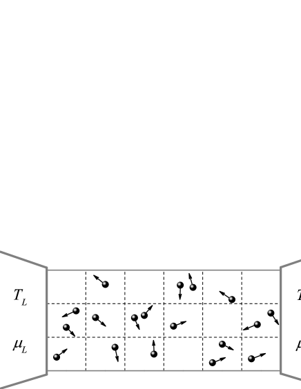
Figure 1: Schematic drawing of the 2D gas of interacting particles, described by the multi-particle collision dynamics. The cells of dashed-line boundaries represent the partition of space used to model collisions. A magnetic field, transverse to the plane of motion, is applied to the system which is coupled to left and right electrochemical reservoirs.

The system is placed in contact with two electrochemical reservoirs at $x=0$ and $x=L$, through openings of the same size as the width $W$ of the box periodic . The left and right reservoirs are modeled as ideal gases and are characterized by temperature $T_{\gamma}$ and electrochemical potential $\mu_{\gamma}$ ($\gamma=L,R$). We use a stochastic model of the reservoirs carlos2001 ; carlos2003 : whenever a particle of the system crosses the boundary which separates the system from the left or right reservoir, it is removed. On the other hand, particles are injected into the system from the boundaries, with rates and energy distribution determined by temperature and electrochemical potential (see, e.g., Benenti2017 ). Thermoelectric transport was discussed with this method Casati2008 ; Saito2010 ; Benenti2013 ; stark ; Chen2015 , also for the MPC model Benenti2014 ; Luo2018 .

We first consider the case $B(x)=gx$. As expected from the above theory, the numerical results of Fig. 2 show that the Onsager symmetry $\Pi(g)=TS(g)$ is fulfilled for any value of $g$ (together with the Onsager-Casimir relation $\Pi(g)=TS(-g)$, this implies that the thermopower $S(g)$ and the Peltier coefficient $\Pi(g)$ are even functions). In the inset, we show the relative error $\epsilon_{r}\equiv|\Pi(g)-TS(g)|/\Pi(g)$ for $g=0.3$. We can see that $\epsilon_{r}$, due to the finite integration time $t$ in numerical simulations, decreases $\propto 1/\sqrt{t}$, as expected for statistical errors, and is smaller that $0.3\%$ for $t=1.2\times 10^{8}$.

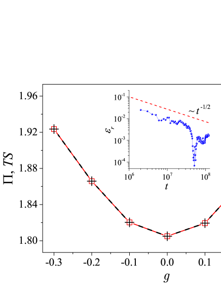
Figure 2: Peltier coefficient $\Pi$ (red open squares) and thermopower $S$ times temperature $T$ (black pluses) as a function of $g$, for a field $B(x)=gx$. Parameter values for the MPC simulations: lenght $L=10$, width $W=2$, side of the square cells $a=0.1$, time between collisions $\tau=0.25$, rotation angle $\alpha=\pi/2$, temperature $T=1$, and particle density $\rho=22$ (the electrochemical potential is set to be $\mu=0$ for $\rho=22$ and $T=1$); the temperature and the electrochemical potential of the left (right) reservoir are, respectively, $T_{L}=T+\Delta T/2$ ($T_{R}=T-\Delta T/2$) and $\mu_{L}=\mu+\Delta\mu/2$ ($\mu_{R}=\mu-\Delta\mu/2$) with $\Delta T=0.05$ and $\Delta\mu=0.05$. Inset: relative error $\varepsilon_{r}=|\Pi(g)-TS(g)|/\Pi(g)$ for $g=0.3$ versus integration time $t$ for $g=0.3$.

We then consider the generic case and numerically investigate several functions $B(x,y)$, without finding any statistically significant violation of the Onsager symmetry. As an illustrative example, in Fig. 3 we show results for $B(x,y)=g\sin[\pi x/(2L)]\sin[\pi y/(2W)]$. Similarly to the case of Fig. 2, the Onsager symmetry is fulfilled, with the relative error $\epsilon_{r}\propto 1/\sqrt{t}$ (see the inset, where we show as an example $g=3$, for wich $\epsilon_{r}$ is smaller that $0.5\%$ for $t=1.4\times 10^{7}$.

Discussion and conclusions.– We have analytically shown that, for systems in a magnetic field of strength varying along one direction, there exists a symmetry such that the equations of motion are invariant under time reversal without reversing the magnetic field. As a consequence of such symmetry of the microscopic dynamics, the Onsager reciprocal relations for the phenomenological transport coefficients remain valid. On the other hand, extensive numerical simulations carried out on two-dimensional systems suggest that the symmetry persists for a generic $B(x,y)$ magnetic field. This result can be qualitatively understood from the following argument rondoni . The field $B(x,y)$ can be approximated by a finite number $n$ of step functions (in the $y$ direction), $B(x,y)\approx B(x,y_{k})$ for step $k$ ($k=1,...,n$). For each step the magnetic field is constant in the $y$ direction, and therefore the above symmetry applies. On the other hand, discontinuities of the field between steps would induce sudden changes of velocity but not affect the symmetry. The results of this paper could be extended to quantum mechanics, with the proper counterpart of map ${\cal M}$ of Eq. (2) discussed in Ref. rondoni2017 . The question remains, for three-dimensional motion, if the Onsager symmetry applies also for a magnetic field with both strength and direction depending on position. We conjecture a positive answer on the basis of the following argument. One could divide the system into small volumes $dV_{\alpha}$ and for each volume approximate the magnetic field with a constant vector. Building a local Cartesian tern $(x_{\alpha},y_{\alpha},z_{\alpha})$ for each $dV_{\alpha}$, with $z_{\alpha}$ pointing in the field direction, symmetry (2) applies locally. For $dV_{\alpha}\to 0$, we expect to obtain a time-reversal trajectory without reversing the magnetic field unpublished .

The results of this paper have consequences on the thermodynamic bounds imposed on the efficiency of coupled transport. The Onsager symmetry is a severe thermodynamic constraint to the efficiency of (thermoelectric) energy conversion, and for that reason it was suggested that a magnetic field, breaking that symmetry, might be useful to enhance the performance of a thermoelectric device Benenti2011 . The results of the present paper exclude such possibility for two-terminal devices coriolis , not only for noninteracting systems datta but in general transport models with strong particle-particle interactions.

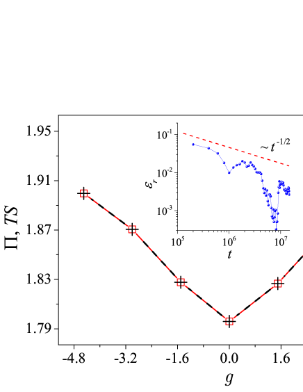
Figure 3: Same as in Fig.2, but for the magnetic field $B(x,y)=g\sin[\pi x/(2L)]\sin[\pi y/(2W)]$. Parameter values are the same as for Fig.2. Inset: relative error $\epsilon_{r}$ vs. integration time $t$ for $g=3$.

Acknowledgments: We thank Keiji Saito for bringing to our attention Ref. rondoni2014 and Lamberto Rondoni for useful discussions. We acknowledge support by NSFC (Grants No. 11535011 and No. 11335006) and by the INFN through the project QUANTUM.

References

- (1) L. Onsager, Phys. Rev. 37, 405 (1931).
- (2) H. B. Callen, Thermodynamics and an Introduction to Thermostatics (2nd ed.) (John Wiley & Sons, New York, 1985).
- (3) S. R. de Groot and P. Mazur, Nonequilibrium Thermodynamics (North-Holland, Amsterdam, 1962).
- (4) G. Benenti, G. Casati, K. Saito, and R. S. Whitney, Phys. Rep. 694, 1 (2017).
- (5) H. B. G. Casimir, Rev. Mod. Phys. 17, 343 (1945).
- (6) S. Datta, Electronic transport in mesoscopic systems (Cambridge University Press, Cambridge, England, 1995).
- (7) S. Bonella, G. Ciccotti, and L. Rondoni, EPL 108, 60004 (2014).
- (8) P. De Gregorio, S. Bonella, and L. Rondoni, Symmetry 9, 120 (2017).
- (9) Our question refers to Hamiltonian systems. We do not consider here systems exposed to inelastic scattering events, for which it is known that it is possible to have Saito2011 ; Sanchez2011 ; Horvat2012 ; Vinitha2013 ; Brandner2013a ; Brandner2013b ; Brandner2015 ; Yamamoto2016 .
- (10) A. Malevanets and R. Kapral, J. Chem. Phys. 110, 8605 (1990).
- (11) In the direction, the particles are subject to fixed (hard wall) boundary conditions. On the other hand, it has been verified numerically that the symmetry discussed in this paper remains valid for periodic boundary conditions.
- (12) C. Mejía-Monasterio, H. Larralde, and F. Leyvraz, Phys. Rev. Lett. 86, 5417 (2001).
- (13) H. Larralde, F. Leyvraz, and C. Mejía-Monasterio, J. Stat. Phys. 113, 197 (2003).
- (14) G. Casati, C. Mejía-Monasterio, and T. Prosen, Phys. Rev. Lett. 101, 016601 (2008).
- (15) K. Saito, G. Benenti, and G. Casati, Chem. Phys. 375, 508 (2010).
- (16) G. Benenti, G. Casati, and J. Wang, Phys. Rev. Lett. 110, 070604 (2013).
- (17) J. Stark, K. Brandner, K. Saito, and U. Seifert, Phys. Rev. Lett. 112, 140601 (2014).
- (18) S. Chen, J. Wang, G. Casati, and G. Benenti, Phys. Rev. E 92, 032139 (2015).
- (19) G. Benenti, G. Casati, and C. Mejía-Monasterio, New J. Phys. 16, 015014 (2014).
- (20) R. Luo, G. Benenti, G. Casati, and J. Wang, Phys. Rev. Lett. 121, 080602 (2018).
- (21) This argument develops a suggestion by L. Rondoni (private communication).
- (22) Numerical investigations to check our conjecture are under way.
- (23) G. Benenti, K. Saito, and G. Casati, Phys. Rev. Lett. 106, 230602 (2011).
- (24) The question remains for other time-reversal breaking mechanisms like the Coriolis force.
- (25) K. Saito, G. Benenti, G. Casati, and T. Prosen, Phys. Rev. B 84, 201306(R) (2011).
- (26) D. Sánchez and L. Serra, Phys. Rev. B 84, 201307(R) (2011).
- (27) M. Horvat, T. Prosen, G. Benenti, and G. Casati, Phys. Rev. E 86, 052102 (2012).
- (28) V. Balachandran, G. Benenti, and G. Casati, Phys. Rev. B 87, 165419 (2013).
- (29) K. Brandner, K. Saito, and U. Seifert, Phys. Rev. Lett. 110, 070603 (2013).
- (30) K. Brandner and U. Seifert, New J. Phys. 15, 105003 (2013).
- (31) K. Brandner and U. Seifert, Phys. Rev. E 91, 012121 (2015).
- (32) K. Yamamoto, O. Entin-Wohlman, A. Aharony, and N. Hatano, Phys. Rev. B 94, 121402(R) (2016).