Efficient passive measurement-device-independent quantum key distribution

Abstract

The measurement-device-independent quantum key distribution (MDI-QKD) possesses the highest security among all practical quantum key distribution protocols. However, existing multi-intensity decoy-state methods may cause loopholes when modulating light intensities with practical devices. In this paper, we propose a passive decoy-state MDI-QKD protocol based on a novel structure of heralded single-photon sources. It does not need to modulate the light source into different intensities and thus can avoid leaking modulation information of decoy states to eavesdroppers, enhancing the security of practical MDI-QKD. Furthermore, by combining the passive decoy states and biased basis choices, our protocol can exhibit distinct advantages compared with state-of-the art MDI-QKD schemes even when the finite key-size effect is taken into account. Therefore, our present passive decoy-state MDI-QKD seems a promising candidate for practical implementation of quantum key distributions in the near future.

I Introduction

Quantum key distribution (QKD) BB84 ; E91 allows legitimate users, Alice and Bob, to share secret keys under unprecedented level of security based on quantum mechanics. Its unconditional security has been proven with ideal devices Mayers ; Lo1 ; Shor . However, the device imperfections in reality offers opportunities for eavesdropper, Eve, to launch quantum hacking PNS ; Blind ; Gerhardt . Fortunately, some countermeasures are invented to fix these security loopholes, such as decoy-state method Hwang ; WXB2005 ; Lo2 and measurement-device-independent QKD (MDI-QKD) Braunstein ; Lo3 .

In most experimental demonstrations of decoy-state QKD Qin1 ; WangS ; Boaron421 ; RFIMDI ; Yin404 , people actively modulate light sources into different intensities with acousto- or electro-optic modulators. However, there may exist side-channel loopholes during the intensity modulation processes. For example, when a modulator is not properly designed, some physical parameters of the pulses emitted by the sender may depend on the particular setting selected Curty1 ; HuJZ , causing severe security problems. To reduce the information leakage, some passive decoy-state methods have been put forward Mauerer ; Adachi ; Qin2 ; Curty2 ; Qin3 and experimentally demonstrated SunSH ; Qin4 ; Qin5 .

However, in practical implementations of MDI-QKD WXB1 ; WXB2 ; LSA ; Curty3 ; WXB3 ; WXB4 ; WXB5 ; Qin6 ; WXB6 , only active decoy-state methods are adopted. It is mainly due to the fact that in most passive schemes the vacuum state cannot be directly observed and also hard to precisely estimate with those observed data. To solve the problem, in this paper we propose an improved passive decoy-state MDI-QKD protocol. It is based on a novel structure of heralded single-photon sources (HSPS) presented in our recent work Qin2 ; Qin4 , by combining the idea of scaling in WXB6 , we are able to give more precise parameter estimations with the data that can be observed in experiment. Through carrying out full parameter optimizations, we do investigation on its performance with finite-size-key effects. Corresponding simulation results demonstrate that our present scheme can work more efficiently than state-of-the art decoy-state MDI-QKD scheme using WCS WXB4 , and can even show some advantages compared with the most advanced MDI-QKD scheme using HSPS WXB6 .

II Passive decoy-state MDI-QKD protocol

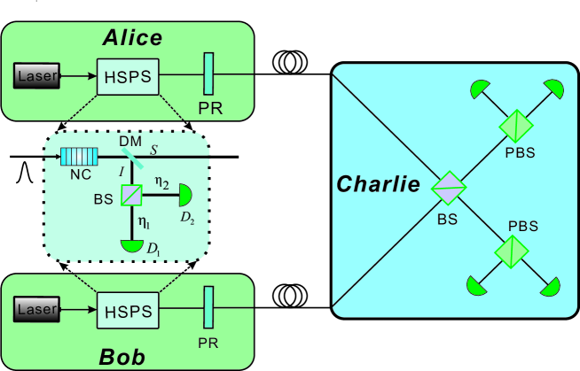
Figure 1: The schematic of our passive decoy-state MDI-QKD protocol. HSPS, heralded single-photon source; NC, nonlinear crystal; DM, dichroic mirror; BS, beam splitter; PBS, polarization beam-splitter; PR, polarization rotator; $D_{1}$ and $D_{2}$, single-photon detectors.

Our passive decoy-state MDI-QKD protocol is presented in Fig. 1. At Alice’s (Bob’s) side, a time correlated pulse pair from parametric down-conversion (PDC) process of nonlinear crystal is split into idler mode $I$ and signal mode $S$. The mode $I$ is further split and then measured by two local detectors, while mode $S$ is encoded conditionally on the local detection events and sent to untrustworthy third party (UTP), Charlie, for bell state measurement (BSM). The local detection events can be divided into four kinds, denoted as $V_{i}$ $(i=1,2,3,4)$: (1) Non-clicking; (2) Single clicking at $D_{1}$; (3) Single clicking at $D_{2}$; (4) Clicking at both $D_{1}$ and $D_{2}$. These events $V_{i}$ correspond to projected state $l$ $(l=w,x,y,z)$ of mode $S$ in the photon-number space. In our protocol, when $V_{i}$ event happens, the signal mode $S$ will be encoded on specific basis, i.e., state $w$ and $x$ are only prepared in $X$ basis while state $y$ and $z$ only prepared in $Z$ basis. The data on $X$ basis is used to estimate channel parameter, and the data on $Z$ basis is used to distill keys. The nomenclature and corresponding relationship is shown in Table 1.

Table 1: The nomenclature and corresponding relationship in our protocol.

Events	State	Probability	Encoding basis
$V_{1}$	$w$	$P_{n}^{w}$	$X$
$V_{2}$	$x$	$P_{n}^{x}$	$X$
$V_{3}$	$y$	$P_{n}^{y}$	$Z$
$V_{4}$	$z$	$P_{n}^{z}$	$Z$

Condition on event $V_{i}$, the mode $S$ is projected into the photon-number space ${\rho_{l}}=\sum\nolimits_{n}{P_{n}^{l}|n\rangle\langle n|}$, and the photon number statistics can be expressed as Qin2

$$P_{n}^{l}={P_{n}}\sum\limits_{{s_{1}}{s_{2}}}{{P_{{V_{i}}|{s_{1}}{s_{2}}}}{P_{{s_{1}}{s_{2}}|n}}},$$ (1)

where $P_{n}$ is the photon-number distribution of PDC process; $P_{s_{1}s_{2}|n}$ denotes the projecting probability of $n$-photon state passing through the BS and being projected into state $|s_{1}s_{2}\rangle$; $P_{V_{i}|s_{1}s_{2}}$ denotes the probability of an $V_{i}$ event given a projected state $|s_{1}s_{2}\rangle$. Note that $P_{n}$ can be certain distribution of PDC process, here we assume a Poisson distribution, i.e., ${P_{n}}=\frac{{{\mu^{n}}}}{{n!}}{e^{-\mu}}$, where $\mu$ is the mean photon number of idler mode or signal mode. Besides, all $P_{V_{i}|s_{1}s_{2}}$ are listed in Table 2, while $P_{s_{1}s_{2}|n}$ is given by Qin2

$${P_{{s_{1}}{s_{2}}|n}}=\sum\limits_{k=0}^{n}{\sum\limits_{{s_{2}}=0}^{n-k}{\sum\limits_{{s_{1}}=0}^{k}{\frac{{n!{t^{k}}{{\left({1-t}\right)}^{n-k}}\eta_{1}^{{s_{1}}}\eta_{2}^{{s_{2}}}{{\left({1-{\eta_{1}}}\right)}^{k-{s_{1}}}{\left({1-{\eta_{2}}}\right)^{n-k-{s_{2}}}}}}}{{{s_{1}}!{s_{2}}!\left({k-{s_{1}}}\right)!\left({n-k-{s_{2}}}\right)!}}}}},$$ (2)

where $t$ represents the transmission efficiency of the BS, reasonably assume $t\in(0,{{\textstyle{1\over 2}}})$; $\eta_{1}$ and $\eta_{2}$ denote the overall efficiency of each branch in the idler mode respectively, which includes the detection efficiency but excludes the transmission efficiency of the BS ($t$); $d_{1}$ and $d_{2}$ refer to the dark count rate of $D_{1}$ and $D_{2}$.

Table 2: Probability of the $V_{i}$ event occurring.

Case	$P_{V_{1}|s_{1}s_{2}}$	$P_{V_{2}|s_{1}s_{2}}$	$P_{V_{3}|s_{1}s_{2}}$	$P_{V_{4}|s_{1}s_{2}}$
$s_{1}=0,s_{2}=0$	$(1-d_{1})(1-d_{2})$	$d_{1}(1-d_{2})$	$d_{2}(1-d_{1})$	$d_{1}d_{2}$
$s_{1}\neq 0,s_{2}=0$	0	$1-d_{2}$	0	$d_{2}$
$s_{1}=0,s_{2}\neq 0$	0	0	$1-d_{1}$	$d_{1}$
$s_{1}\neq 0,s_{2}\neq 0$	0	0	0	1

In the MDI-QKD, Alice and Bob simultaneously send photon pulses to the UTP. When Alice sends state $l$ and and Bob sends state $r$ $(l,r\in\{w,x,y,z\})$, we can obtain the gains ${S_{lr}}=\sum\nolimits_{j,k\geqslant 0}{a_{j}^{l}b_{k}^{r}{Y_{jk}}}$, and quantum bit errors ${\kern 1.0pt}{T_{lr}}=\sum\nolimits_{j,k\geqslant 0}{a_{j}^{l}b_{k}^{r}{Y_{jk}}{e_{jk}}}$. Here $a_{j}^{l}$ and $b_{k}^{r}$ are the probability distribution as presented in Eq. (1) at Alice’s side and Bob’s side, respectively. $Y_{jk}$ and $e_{jk}$ each denotes the yield and the error rate when Alice sends a $j$-photon state and Bob sends a $k$-photon state. The average quantum-bit error-rate (QBER) is given by ${E_{lr}}={{{T_{lr}}}\mathord{\left/{\vphantom{{{T_{lr}}}{{S_{lr}}}}}\right.\kern-1.2pt}{{S_{lr}}}}$. From Ref. Qin2 ; WXB1 , we know that former formulae used to estimate the yield and error rate of single-photon pair in $X$ basis are

$$Y_{11}^{X,L}=\frac{{a_{1}^{x}b_{2}^{x}\left({\underline{S}_{ww}-\overline{{\cal H}}}\right)-a_{1}^{w}b_{2}^{w}\left({\overline{S}_{xx}-\underline{{\cal H}}^{\prime}}\right)}}{{a_{1}^{w}a_{1}^{x}(b_{1}^{w}b_{2}^{x}-b_{1}^{x}b_{2}^{w})}},\quad e_{11}^{X,U}=\frac{{\overline{T}_{ww}-{\textstyle{1\over 2}}\underline{{\cal H}}}}{{a_{1}^{w}b_{1}^{w}Y_{11}^{X,L}}},$$ (3)

where ${\cal H}\equiv a_{0}^{w}b_{0}^{w}{Y_{00}}+\sum\nolimits_{m=1}^{\infty}{(a_{0}^{w}b_{m}^{w}{Y_{0m}}+a_{m}^{w}b_{0}^{w}{Y_{m0}})}$, ${\cal H}^{\prime}\equiv a_{0}^{x}b_{0}^{x}{Y_{00}}+\sum\nolimits_{m=1}^{\infty}{(a_{0}^{x}b_{m}^{x}{Y_{0m}}+a_{m}^{x}b_{0}^{x}{Y_{m0}})}$; $L$ and $U$ refer to the lower bound and upper bound, respectively. Besides, we denote overline and underline as the experimental values with statistical fluctuation. For example, for experimental value of ${S_{ww}}$, it satisfies ${\underline{S}_{ww}}:={S_{ww}}-{\Delta_{1}}\leqslant{\widetilde{S}_{ww}}\leqslant{\overline{S}_{xx}}:={S_{xx}}+{\Delta_{2}}$ with a failure probability $\varepsilon$, where $\Delta_{1}$ and $\Delta_{2}$ are the statistical fluctuation values.

However, in fact, the experimental values related to vacuum state presented in Eq. (3), i.e., ${\cal H}$ and ${\cal H}^{\prime}$, cannot be directly measured in our passive MDI-QKD protocol. Fortunately, we can borrow the idea in WXB6 to reformulate Eq. (3) as

$$\widetilde{Y}_{11}^{X,L}(\widetilde{{\cal H}})=\frac{{a_{1}^{x}b_{2}^{x}{\underline{S}_{ww}}-a_{1}^{w}b_{2}^{w}{\overline{S}_{xx}}-a_{1}^{x}b_{2}^{x}\widetilde{{\cal H}}}}{{a_{1}^{w}a_{1}^{x}(b_{1}^{w}b_{2}^{x}-b_{1}^{x}b_{2}^{w})}},$$ (4)

and

$$\widetilde{e}_{11}^{X,U}(\widetilde{{\cal H}})=\frac{{\overline{T}_{ww}-{\textstyle{1\over 2}}\widetilde{{\cal H}}}}{{a_{1}^{w}b_{1}^{w}\widetilde{Y}_{11}^{X,L}(\widetilde{{\cal H}})}}.$$ (5)

where $\widetilde{{\cal H}}$ is the value of ${\cal H}$, which is a joint parameter existing in $Y_{11}$ and $e_{11}$. According to the $\widetilde{e}_{11}^{X,U}(\widetilde{{\cal H}})$ in Eq. (5), we can obviously have the range of $\widetilde{{\cal H}}$ as

$$\widetilde{{\cal H}}\in\left[{0,2{\overline{T}_{ww}}}\right].$$ (6)

In our protocol, we use the data in $X$ basis to estimate the channel parameters in $Z$ basis ($Y_{11}^{Z}$ and $e_{11}^{ph}$), but their real values in $Z$ basis may deviate from the quantities in $X$ basis. Therefore, a stricter treatment should be taken here. We use

$$-{\Delta_{1}^{\prime}}\leqslant Y_{11}^{Z}(\widetilde{{\cal H}})-\widetilde{Y}_{11}^{X,L}(\widetilde{{\cal H}})\leqslant{\Delta_{2}^{\prime}},$$ (7)

$$-{\Delta_{1}^{\prime\prime}}\leqslant e_{11}^{ph}(\widetilde{{\cal H}})-\widetilde{e}_{11}^{X,U}(\widetilde{{\cal H}})\leqslant{\Delta_{2}^{\prime\prime}},$$ (8)

for the worst-case values of $Y_{11}^{Z,L}(\widetilde{{\cal H}})$ and $e_{11}^{ph,U}(\widetilde{{\cal H}})$ with a failure probability.

With the above formulae, we shall estimate the worst-case result for the key rate by scanning all possible values of ${\widetilde{{\cal H}}}$ given in Eq. (6), and get the final key generation rate per pulse as

$$R\geqslant\mathop{min}\limits_{\widetilde{{\cal H}}}R(\widetilde{{\cal H}})=\left\{{a_{1}^{y}b_{1}^{y}Y_{11}^{Z,L}(\widetilde{{\cal H}})\left[{1-{H_{2}}\left({e_{11}^{ph,U}(\widetilde{{\cal H}})}\right)}\right]-S_{yy}^{Z}f{H_{2}}\left({E_{yy}^{Z}}\right)}\right\}-\frac{1}{{{N_{t}}}}\left({{{\log}_{2}}\frac{8}{{{\epsilon_{cor}}}}+2{{\log}_{2}}\frac{2}{{\varepsilon^{\prime}\hat{\varepsilon}}}+2{{\log}_{2}}\frac{1}{{{\varepsilon_{PA}}}}}\right),$$ (9)

where $f$ is the inefficiency of error correction; $H_{2}(p)=-p\log_{2}(p)-(1-p)\log_{2}(1-p)$ is the binary Shannon entropy function. The second part of Eq. (9) is due to other finite size effects on the key rate as defined in Curty3 , guaranteeing the composable security of whole MDI-QKD system. Note that here we only use the state $y$ conditional on event $V_{3}$ to generate keys. Though we can also use state $z$ to distill keys, our numerical simulation shows that it raise the key rate little because the probability of event $V_{4}$ is very low compared with event $V_{3}$.

III Simulation RESULTS

In the following, we carry out numerical simulations for our proposed passive decoy-state MDI-QKD protocol. Here, we focus on the symmetric case, which means that Charlie is at the middle of Alice and Bob, and all other device parameters of Alice’s side and Bob’s side are identical. Let $d_{1}=d_{2}=d_{A}$ and $\eta_{1}=\eta_{2}=\eta_{A}$, we can obtain the simplified photon-number distribution for $a_{n}^{l},b_{n}^{r}$ ($l,r\in\{w,x,y,z\}$) as

$$\begin{array}[]{l}P_{n}^{w}={(1-{d_{A}})^{2}}{(1-{\eta_{A}})^{n}}\frac{{{\mu^{n}}}}{{n!}}{e^{-\mu}},\\ P_{n}^{x}=(1-{d_{A}}){(1-{\eta_{A}})^{n}}\left[{{{\left({\frac{{1-(1-t){\eta_{A}}}}{{1-{\eta_{A}}}}}\right)}^{n}}+{d_{A}}-1}\right]\frac{{{\mu^{n}}}}{{n!}}{e^{-\mu}},\\ P_{n}^{y}=(1-{d_{A}}){(1-{\eta_{A}})^{n}}\left[{{{\left({\frac{{1-t{\eta_{A}}}}{{1-{\eta_{A}}}}}\right)}^{n}}+{d_{A}}-1}\right]\frac{{{\mu^{n}}}}{{n!}}{e^{-\mu}},\\ P_{n}^{z}=\frac{{{\mu^{n}}}}{{n!}}{e^{-\mu}}-P_{n}^{w}-P_{n}^{x}-P_{n}^{y}.\end{array}$$ (14)

Here, the Eq. (14) needs to satisfy the condition ${\textstyle{{{P_{n}^{x}}}\over{{P_{n}^{w}}}}}\geqslant{\textstyle{{{P_{2}^{x}}}\over{{P_{2}^{w}}}}}\geqslant{\textstyle{{{P_{1}^{x}}}\over{{P_{1}^{w}}}}}$ for $n\geqslant 3$ to let Eq. (4) hold, and the proof of this condition has been given in Qin2 .

Table 3: The device parameters used in our numerical simulations. $e_{0}$, the error rate of vacuum pulses; $e_{d}$, the misalignment error; $\eta_{A}$ and $d_{A}$, the overall efficiency and the dark count rate of the local detector at Alice (or Bob)’s side; $\eta_{C}$ and $d_{C}$ each corresponds to the detection efficiency and the dark count rate of detectors at the Charlie’s side; $f$, the inefficiency of error correction.

$e_{0}$	$e_{d}$	$\eta_{A}$	$d_{A}$	$\eta_{C}$	$d_{C}$	$f$
0.5	1.5%	75%	$10^{-6}$	40%	$10^{-7}$	1.16

In our simulation, we use the commonly used loss coefficient of 0.2 dB/km, and other device parameters are listed in Table 3. We make comparisons between our present work and other two representative active MDI-QKD schemes WXB4 ; WXB6 , in which Ref. WXB6 is the best active MDI-QKD scheme so far. Furthermore, due to the finite-size key effect, we adopt the same statistical fluctuation method (normal distribution given the failure probability $\varepsilon=10^{-7}$) and composable security level as in WXB6 . Besides, we perform full parameter optimization for all schemes in comparisons. In our protocol, it includes mean photon number $\mu$, transmission efficiency $t$ of the local BS, and the joint parameter $\widetilde{{\cal H}}$. The comparisons are shown in Figs. 2 $\sim$ 4.

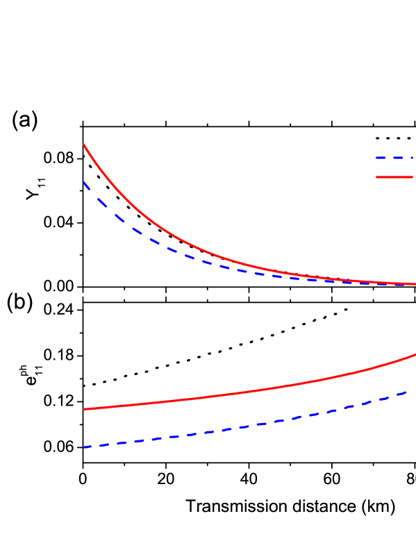
Figure 2: The single-photon-pair yield ($Y_{11}$) and phase-flip error rate ($e_{11}^{ph}$) of different schemes. Here the data size $N_{t}=10^{9}$.

We first plot the comparisons for two key channel parameters, i.e., the yield and the phase-flip error rate of single-photon pairs, between our protocol and other two schemes in Fig. 2. Here the data size of the pulse number each side sends is reasonably set as $N_{t}=10^{9}$. Fig. 2 (a) shows that $Y_{11}$ is estimated more accurately in our passive protocol than other two active schemes, which mainly attributes to that the local detection structure provides some photon-number-resolution ability, while Fig. 2 (b) shows the estimated $e_{11}^{ph}$ of our protocol is in the middle of other two schemes. Finally, the comparisons of key rates for different schemes are illustrated in Fig. 3. It shows that our protocol always outperforms Ref. WXB4 at this data size, and will be advantageous at a relatively longer transmission distance compared with Ref. WXB6 , i.e., $>30$ km.

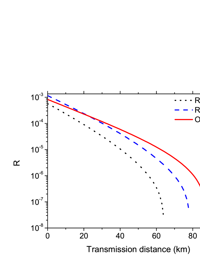
Figure 3: The key rates of our scheme and other two reports at data size $N_{t}=10^{9}$.

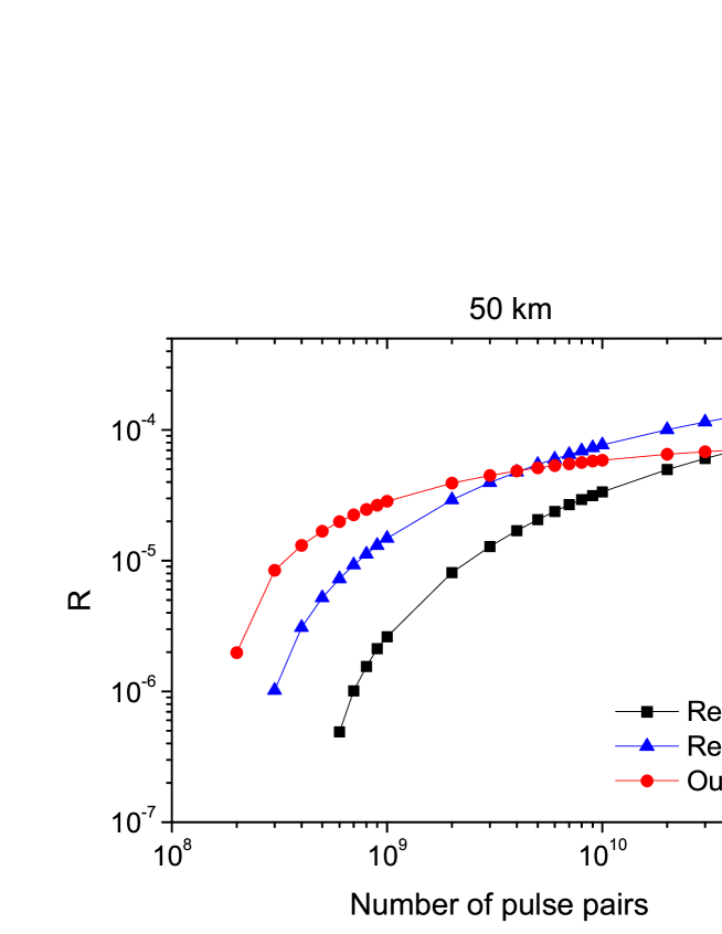
Figure 4: The key rates of different schemes versus data size at 50 km.

Besides, we also investigate the key generation rate changing with the variation of the data size at fixed transmission distance (50 km), as shown in Fig. 4. From Fig. 4, we find that our present work has cross points with the other two state-of-the art MDI-QKD works using either WCS and HSPS, and show best performance at small data size, e.g., $N_{t}\leqslant 4\times 10^{9}$. Compared with Ref. WXB4 , the improvement mainly due to the inherent merit of the sources as explained in Ref. Qin7 . However, even when using the same light sources, HSPS, our work can still exhibit less sensitivity than Ref. WXB6 , making it very promising candidate for practical applications.

IV Conclusions and Discussions

In this paper, we propose a passive decoy-state MDI-QKD protocol, which is impossible for Eve to distinguish between decoy and signal states, enhancing the security of MDI-QKD. The passive decoy states conditional on local events combining the biased basis choice and the idea of scaling in WXB6 are adopted to estimate channel parameters more accurately. Furthermore, we perform full parameter optimization for our protocol, and simulation results show that our protocol can show some advantages even compared with some state-of-the art MDI-QKD schemes, especially at a longer distance or a smaller data size. Hence, our present work provides an alternative and useful approach to improve both the security and practicability of MDI-QKD protocols, and represents a further step along practical implementations of quantum key distributions.

References

- (1) C. H. Bennett, and G. Brassard, Quantum cryptography: public key distribution and coin tossing, in Proceedings of the IEEE International Conference on Computers, Systems and Signal Processing (IEEE, New York, 1984), pp. 175-179.
- (2) A. K. Ekert, Quantum cryptography based on Bell’s theorem, Phys. Rev. Lett. 67, 661 (1991).
- (3) D. Mayers, Unconditional security in quantum cryptography, Journal of the ACM (JACM) 48, 351 C-406 (2001).
- (4) H. K. Lo and H. F. Chau, Unconditional security of quantum key distribution over arbitrarily long distances, Science, 283, 2050 (1999).
- (5) P. W. Shor and J. Preskill, Simple proof of security of the BB84 quantum key distribution protocol, Phys. Rev. Lett. 85, 441 (2000).
- (6) B. Huttner, N. Imoto, N. Gisin, and T. Mor, Quantum cryptography with coherent states, Phys. Rev. A 51, 1863 (1995).
- (7) L. Lydersen, C. Wiechers, C. Wittmann, D. Elser, J. Skaar and V. Makarov, Hacking commercial quantum cryptography systems by tailored bright illumination. Nature Photon. 4, 686 C689 (2010).
- (8) I. Gerhardt, Q. Liu, A. L. Linares, J. Skaar, C. Kurtsiefer, and V. Makarov, Full-field implementation of a perfect eavesdropper on a quantum cryptography system. Nature Commun. 2, 349 (2011).
- (9) W. Y. Hwang, Quantum Key Distribution with High Loss: Toward Global Secure Communication, Phys. Rev. Lett. 91, 057901 (2003).
- (10) X. B. Wang, Beating the Photon-Number-Splitting Attack in Practical Quantum Cryptography, Phys. Rev. Lett. 94, 230503 (2005).
- (11) H. K. Lo, X. Ma, K. Chen, Decoy State Quantum Key Distribution, Phys. Rev. Lett. 94, 230504 (2005).
- (12) S. L. Braunstein and S. Pirandola, Side-Channel-Free Quantum Key Distribution, Phys. Rev. Lett. 108, 130502 (2012).
- (13) H. K. Lo, M. Curty, and B. Qi, Measurement-Device-Independent Quantum Key Distribution, Phys. Rev. Lett. 108, 130503 (2012).
- (14) Q. Wang, W. Chen, G. Xavier, M. Swillo, T. Zhang, S. Sauge, M. Tengner, Z. F. Han, G. C. Guo, and A. Karlsson, Experimental decoy-state quantum key distribution with a sub-poissionian heralded single-photon source, Phys. Rev. Lett. 100, 090501 (2008).
- (15) S. Wang, W. Chen, Z. Q. Yin, D. Y. He, C. Hui, P. L. Hao, G. J. Fan-Yuan, C. Wang, L. J. Zhang, J. Kuang, S. F. Liu, Z. Zhou, Y. G. Wang, G. C. Guo, and Z. F. Han, Practical gigahertz quantum key distribution robust against channel disturbance, Opt. Lett. 43, 2030–2033 (2018).
- (16) A. Boaron, G. Boso, D. Rusca, C. Vulliez, C. Autebert, M. Caloz, M. Perrenoud, G. Gras, F. Bussieres, M. J. Li, D. Nolan, A. Martin, and H. Zbinden, Secure Quantum Key Distribution over 421 km of Optical Fiber, Phys. Rev. Lett. 121, 190502 (2018).
- (17) C. Wang, X. T. Song, Z. Q. Yin, S. Wang, W. Chen, C. M. Zhang, G. C. Guo, and Z. F. Han, Phase-Reference-Free Experiment of Measurement-Device-Independent Quantum Key Distribution, Phys. Rev. Lett. 115, 160502 (2015).
- (18) H. L. Yin, T. Y. Chen, Z. W. Yu, H. Liu, L. X. You, Y. H. Zhou, S. J. Chen, Y. Mao, M. Q. Huang, W. J. Zhang, H. Chen, M. J. Li, D. Nolan, F. Zhou, X. Jiang, Z. Wang, Q. Zhang, X. B. Wang, and J. W. Pan, Measurement-device-independent quantum key distribution over a 404 km optical fiber, Phys. Rev. Lett. 117, 190501 (2016).
- (19) M. Curty, X. Ma, B. Qi, and T. Moroder, Passive decoy-state quantum key distribution with practical light sources. Phys. Rev. A 81, 022310 (2010).
- (20) J. Z. Hu and X. B. Wang, Reexamination of the decoy-state quantum key distribution with an unstable source, Phys. Rev. A 82, 012331 (2010).
- (21) W. Mauerer and C. Silberhorn, Quantum key distribution with passive decoy state selection, Phys. Rev. A 75, 050305(R) (2007).
- (22) Y. Adachi, T. Yamamoto, M. Koashi, and N. Imoto. Simple and efficient quantum key distribution with parametric down-conversion, Phys. Rev. Lett. 99, 180503 (2007).
- (23) M. Curty, M. Jofre, V. Pruneri, and M. W. Mitchell, Passive decoy-state quantum key distribution with coherent light, Entropy 17, 4064–4082 (2015).
- (24) Q. Wang, C. H. Zhang, X. B. Wang, Scheme for realizing passive quantum key distribution with heralded single-photon sources, Phys. Rev. A 93, 032312 (2016).
- (25) C. H. Zhang, D. Wang, C. M. Zhang, and Q. Wang, A simple scheme for realizing the passive decoy-state quantum key distribution, J. Lightwave Technol. 14, 0733 (2018).
- (26) S. H. Sun, G. Z. Tang, C. Y. Li, and L. M. Liang, Experimental demonstration of passive-decoy-state quantum key distribution with two independent lasers, Phys. Rev. A 94, 032324 (2016)
- (27) C. H. Zhang, D. Wang, X. Y. Zhou, S. Wang, L. B. Zhang, Z. Q. Yin, W. Chen, Z. F. Han, G. C. Guo, and Q. Wang, Proof-of-principle demonstration of parametric down-conversion source-based quantum key distribution over 40 dB channel loss, Opt. Express 26, 25921–25933 (2018).
- (28) C. H. Zhang, X. Y. Zhou, H. J. Ding, C. M. Zhang, G. C. Guo, and Q. Wang, Proof-of-principle demonstration of passive decoy-state quantum digital signatures over 200 km, Phys. Rev. Appl. 10, 034033 (2018).
- (29) X. B. Wang, Three-intensity decoy-state method for device-independent quantum key distribution with basis-dependent errors, Phys. Rev. A 87, 012320 (2013).
- (30) Y. H. Zhou, Z. W. Yu, and X. B. Wang, Tightened estimation can improve the key rate of measurement-device-independent quantum key distribution by more than 100%, Phys. Rev. A 89, 052325 (2014).
- (31) F. Xu, H. Xu, and H. K. Lo, Protocol choice and parameter optimization in decoy-state measurement-device-independent quantum key distribution, Phys. Rev. A 89, 052333 (2014).
- (32) M. Curty, F. Xu, W. Cui, C. C. W. Lim, K. Tamaki, and H. K. Lo, Finite-key analysis for measurement-device-independent quantum key distribution, Nat. Commun. 5, 3732 (2014).
- (33) Z. W. Yu,Y. H. Zhou, and X. B. Wang, Statistical fluctuation analysis for measurement-device-independent quantum key distribution with three-intensity decoy-state method, Phys. Rev. A 91, 032318 (2015).
- (34) Y. H. Zhou, Z. W. Yu, and X. B. Wang, Making the decoy-state measurement-device-independent quantum key distribution practically useful, Phys. Rev. A 93, 042324 (2016).
- (35) C. Jiang, Z. W. Yu, and X. B. Wang, Measurement-device-independent quantum key distribution with source state errors and statistical fluctuation, Phys. Rev. A 95, 032325 (2017).
- (36) C. H. Zhang, C. M. Zhang, G. C. Guo, and Q. Wang, Biased three-intensity decoy-state scheme on the measurement-device-independent quantum key distribution using heralded single-photon sources, Opt. Express 26, 004219 (2018).
- (37) X. L. Hu, Z. W. Yu, and X. B. Wang, Efficient measurement-device-independent quantum key distribution without vacuum sources, Phys. Rev. A 98, 032303 (2018).
- (38) X. Y. Zhou, C. H. Zhang, C. M. Zhang, and Q. Wang, Obtaining better performance in the measurement-device-independent quantum key distribution with heralded single-photon sources, Phys. Rev. A 96, 052337 (2017).