TIRA: Toolbox for Interval Reachability Analysis

Abstract.

This paper presents TIRA, a Matlab library gathering several methods for the computation of interval over-approximations of the reachable sets for both continuous- and discrete-time nonlinear systems. Unlike other existing tools, the main strength of interval-based reachability analysis is its simplicity and scalability, rather than the accuracy of the over-approximations. The current implementation of TIRA contains four reachability methods covering wide classes of nonlinear systems, handled with recent results relying on contraction/growth bounds and monotonicity concepts. TIRA’s architecture features a central function working as a hub between the user-defined reachability problem and the library of available reachability methods. This design choice offers increased extensibility of the library, where users can define their own method in a separate function and add the function call in the hub function.

1. Introduction

Reachability analysis aims to compute the set of successor states that can be reached by a system given sets of initial states and admissible inputs. Since an exact computation of a reachable set is not possible for most systems, we rely on methods to over-approximate this set. Various tools and set representations for these over-approximations have been proposed in the literature, such as zonotopes in CORA (Althoff, 2015), support functions in SpaceEx (Frehse et al., 2011), ellipsoids in the Ellipsoidal Toolbox (Kurzhanskiy and Varaiya, 2006), Taylor models in Flow^∗ (Chen et al., 2013), polytopes in Sapo (Dreossi, 2017) or interval pavings (Jaulin et al., 2001). Other tools such as the Level Set Toolbox (Mitchell and Templeton, 2005) are instead designed to tackle backward reachability problems.

The main common point of the above reachability methods is that their primary focus is to compute a set that over-approximates the actual reachable set as tightly as possible. While such approaches are particularly interesting to minimize the conservativeness of the over-approximation in simple verification objectives (e.g. with safety or reachability specifications), the inherent complexity of the set representations allowing for such tight approximations can make these sets impractical to use if further manipulations are required (e.g. saving in memory, intersection with another set).

On the other hand, reachability analysis plays a central role in the field of abstraction-based control synthesis (see e.g. (Moor and Raisch, 2002; Coogan and Arcak, 2015; Reissig et al., 2016; Meyer and Dimarogonas, 2018)), where a reachable set over-approximation needs to be computed for each cell of a state space partition and each input value (i.e. exponential complexity in the state and input dimensions), and the abstraction is obtained by intersecting these sets with the partition elements. In addition, existing abstraction tools are limited by their internal reachability algorithms: e.g. SCOTS (Rungger and Zamani, 2016) relies on the hard-coded growth bound method; PESSOA (Mazo Jr et al., 2010) cannot handle nonlinear systems unless the user provides their own over-approximation function. This motivated recent work (Coogan and Arcak, 2015; Reissig et al., 2016; Meyer et al., 2018; Meyer and Dimarogonas, 2018) on reachability analysis based on the simpler set representation of multi-dimensional intervals (also known as axis-aligned boxes or hyper-rectangles). While intervals usually result in more conservative over-approximations of the reachable sets, they have useful advantages for the implementation of abstraction-based algorithms: they are fully defined with only two state vectors; their intersection is still an interval; the associated over-approximation methods have very good scalability with a complexity (number of successor computations) at best constant (Reissig et al., 2016; Moor and Raisch, 2002; Meyer and Dimarogonas, 2018; Coogan and Arcak, 2015) and at worst linear in the state dimension (Meyer et al., 2018). Therefore, compared to existing reachability analysis tools, the interval-based methods trade off the accuracy of the over-approximating sets for the simplicity and scalability of the reachability analysis, while still resulting in the tightest possible interval over-approximation for some of these methods (Moor and Raisch, 2002; Coogan and Arcak, 2015; Meyer et al., 2018).

In this paper, we introduce TIRA  (Toolbox for Interval Reachability Analysis), a Matlab library gathering several methods to compute interval over-approximations of reachable sets for both continuous- and discrete-time systems. The primary motivation for the introduction of this tool library is to make publicly available some of the more recent results on interval reachability analysis (Coogan and Arcak, 2015; Reissig et al., 2016; Meyer et al., 2018; Meyer and Dimarogonas, 2018) and allow external users an easy access to these methods without requiring them to know the theoretical or implementation details. The architecture of the toolbox features a central function working as a hub between the user-defined reachability problem and the library of available reachability methods. It takes the initial state and input intervals and returns the over-approximation interval, applying either the method requested by the user, or otherwise picking the most suitable one based on the system properties. The motivation for this architecture is to offer an easily extensible library, where users can define their own method in a separate function and then add its call in the hub function.

TIRA currently contains four over-approximation methods covering very wide classes of systems: any system with known Jacobian bounds; and any continuous-time system with constant input functions over the time range of the reachability analysis. The three methods for continuous-time systems are based on contraction/growth bounds (Kapela and Zgliczyński, 2009; Reissig et al., 2016), mixed-monotonicity (Meyer and Dimarogonas, 2018), and sampled-data mixed-monotonicity (Meyer et al., 2018). The unique method for discrete-time systems is based on mixed-monotonicity (Meyer et al., 2018).

The paper is organized as follows. Section 2 introduces notations and formulates the considered reachability problems. Section 3 gives an overview of the implemented over-approximation methods alongside their main limitations and the relevant literature. The toolbox architecture is summarized in Section 4. Finally, Section 5 demonstrates the use of TIRA on numerical examples.

2. Problem formulation

Let $\mathbb{R}$ and $\mathbb{R}^{n}$ be the sets of real numbers and $n$-dimensional real vectors, respectively. $1_{n}$ and $0_{n}$ are $n$-dimensional vectors filled with ones and zeros, respectively. $I_{n}$ is the $n\times n$ identity matrix. Given $a,b\in\mathbb{R}^{n}$, $[a,b]\subseteq\mathbb{R}^{n}$ denotes the $n$-dimensional interval $\{x\in\mathbb{R}^{n}~{}|~{}a\leq x\leq b\}$, using componentwise inequalities. Given a set $X\subseteq\mathbb{R}^{n}$, interval $[a,b]\subseteq\mathbb{R}^{n}$ is said to be a tight interval over-approximation of $X$ if $X\subseteq[a,b]$ and for any strictly included interval $[c,d]\varsubsetneq[a,b]$, we have $X\nsubseteq[c,d]$.

We consider both continuous-time and discrete-time systems with time-varying vector field

(1) $$\dot{x}=f(t,x,p),$$

(2) $$x^{+}=F(t,x,p),$$

with time $t\in\mathbb{R}$, state $x\in\mathbb{R}^{n_{x}}$ and input $p\in\mathbb{R}^{n_{p}}$. For the continuous-time system (1), $\Phi(t;t_{0},x_{0},\mathbf{p})$ denotes the state (assumed to exist and be unique) reached at time $t\geq t_{0}$ by system (1) starting from initial state $x_{0}\in\mathbb{R}^{n_{x}}$ at time $t_{0}\in\mathbb{R}$ and under piecewise continuous input function $\mathbf{p}:[t_{0},+\infty)\rightarrow\mathbb{R}^{n_{p}}$. For a constant input function $\mathbf{p}\equiv p\in\mathbb{R}^{n_{p}}$ over the time range $[t_{0},t]$, we write $\Phi(t;t_{0},x_{0},p)$. $\Phi$ is evaluated through Runge-Kutta methods and the associated errors are currently neglected in TIRA.

Problem 1 (Continuous-time reachability).

Given time range $[t_{0},t_{f}]\subseteq\mathbb{R}$, interval of initial states $[\underline{x},\overline{x}]\subseteq\mathbb{R}^{n_{x}}$ and interval of input values $[\underline{p},\overline{p}]\subseteq\mathbb{R}^{n_{p}}$, find an interval in $\mathbb{R}^{n_{x}}$ over-approximating the reachable set of (1) defined as:

$$R(t_{f};t_{0},[\underline{x},\overline{x}],[\underline{p},\overline{p}])=\\ \{\Phi(t_{f};t_{0},x_{0},\mathbf{p})~{}|~{}x_{0}\in[\underline{x},\overline{x}],\mathbf{p}:[t_{0},t_{f}]\rightarrow[\underline{p},\overline{p}]\}.$$

Problem 2 (Discrete-time reachability).

Given initial time $t_{0}\in\mathbb{R}$, interval of initial states $[\underline{x},\overline{x}]\subseteq\mathbb{R}^{n_{x}}$ and interval of input values $[\underline{p},\overline{p}]\subseteq\mathbb{R}^{n_{p}}$, find an interval in $\mathbb{R}^{n_{x}}$ over-approximating the reachable set of (2) defined as:

$$R(t_{0},[\underline{x},\overline{x}],[\underline{p},\overline{p}])=\{F(t_{0},x_{0},p)~{}|~{}x_{0}\in[\underline{x},\overline{x}],p\in[\underline{p},\overline{p}]\}.$$

All over-approximation methods summarized in the next section rely on the Jacobian (assuming a continuously differentiable vector field) and sensitivity matrices of systems (1) and (2). The state and input Jacobian matrices of (1) are given by the partial derivatives $J_{x}(t,x,p)=\frac{\partial f(t,x,p)}{\partial x}$ and $J_{p}(t,x,p)=\frac{\partial f(t,x,p)}{\partial p}$, respectively. The Jacobian matrices of (2) are similarly obtained by replacing $f$ by $F$. For continuous-time systems (1) with constant input functions on $[t_{0},t_{f}]$, we further define the sensitivity of the trajectories $\Phi$ to variations of the initial state $S_{x}(t_{f};t_{0},x_{0},p)=\frac{\partial\Phi(t_{f};t_{0},x_{0},p)}{\partial x_{0}}$ and to variations of the input value $S_{p}(t_{f};t_{0},x_{0},p)=\frac{\partial\Phi(t_{f};t_{0},x_{0},p)}{\partial p}$.

3. Reachability methods

In this section, we give an overview of the four methods currently implemented in TIRA for the over-approximation of the reachable set of system (1) or (2) by an interval. For more in-depth descriptions and proofs, the reader is referred to the papers mentioned in each of the subsections below.

3.1. Contraction/growth bound

This method holds various names in the literature and can be seen as a particular case of the results in (Kapela and Zgliczyński, 2009) based on logarithmic norms, an extension to time-varying systems of the growth bound approach in (Reissig et al., 2016), or an extension to systems with inputs of the componentwise contraction results in (Arcak and Maidens, 2018). Let $x^{*}=\frac{\underline{x}+\overline{x}}{2}\in\mathbb{R}^{n_{x}}$ and $[x]=\frac{\overline{x}-\underline{x}}{2}\in\mathbb{R}^{n_{x}}$ be the center and half-width of the initial state interval $[\underline{x},\overline{x}]$, respectively. Similarly define $p^{*}$ and $[p]$ for $[\underline{p},\overline{p}]$.

Requirements and limitations

The main result of this approach presented below is limited to continuous-time systems (1) with additive input, i.e. $n_{p}=n_{x}$ and for all $t\in\mathbb{R}$, $x\in\mathbb{R}^{n_{x}}$, $p\in\mathbb{R}^{n_{p}}$:

(3) $$f(t,x,p)=f(t,x,0_{n_{p}})+p.$$

In addition, we assume that we are provided a componentwise contraction/growth matrix defined as follows.

Assumption 3.

Given an invariant state space $X\subseteq\mathbb{R}^{n_{x}}$, there exists $C\in\mathbb{R}^{n_{x}\times n_{x}}$ such that for all $t\in[t_{0},t_{f}]$, $x\in X$ and $i,j\in\{1,\dots,n_{x}\}$ with $j\neq i$ we have:

$$\begin{cases}C_{ii}\geq{J_{x}}_{ii}(t,x,p^{*}),\\ C_{ij}\geq|{J_{x}}_{ij}(t,x,p^{*})|.\end{cases}$$

Method description

We first define a growth bound function $G:\mathbb{R}_{\geq 0}\times\mathbb{R}_{\geq 0}^{n_{x}}\times\mathbb{R}_{\geq 0}^{n_{x}}\rightarrow\mathbb{R}_{\geq 0}^{n_{x}}$:

(4) $$G(\tau,x,p)=e^{C\tau}x+\int_{0}^{\tau}e^{Ct}pdt.$$

Then, an interval over-approximation of the reachable set of (3) is obtained by adding and subtracting $G(t_{f}-t_{0},[x],[p])$ to the successor of (3) from the pair $(x^{*},p^{*})$ of the interval centers.

Proposition 4.

Under Assumption 3 and definition (4), an over-approximation of the reachable set of (3) in Problem 1 is given by:

$$R(t_{f};t_{0},[\underline{x},\overline{x}],[\underline{p},\overline{p}])\subseteq\\ [\Phi(t_{f};t_{0},x^{*},p^{*})-G(t_{f}-t_{0},[x],[p]),\\ \Phi(t_{f};t_{0},x^{*},p^{*})+G(t_{f}-t_{0},[x],[p])].$$

Remarks

The following variations of this approach are also available in TIRA. Firstly, Assumption 3 can be replaced by the existence of a scalar contraction/growth factor $c\in\mathbb{R}$ upper bounding the logarithmic norm (associated to any matrix norm) of $J_{x}(t,x,p^{*})$,

$$c\geq\lim_{h\rightarrow 0^{+}}\frac{\|I_{n_{x}}+hJ_{x}(t,x,p^{*})\|-1}{h},\quad\forall t\in[t_{0},t_{f}],~{}x\in X,$$

which can then be used directly in the growth bound definition (4) and Proposition 4, replacing matrix $C$ by scalar $c$ (Kapela and Zgliczyński, 2009).

Secondly, for general dynamics (1) without the additive input assumption from (3), Proposition 4 is modified by replacing $[p]$ by a user-provided vector $\tilde{p}\in\mathbb{R}_{\geq 0}^{n_{x}}$ bounding the influence of the input on the dynamics (using componentwise $\geq$ and $|\cdot|$ operators) (Kapela and Zgliczyński, 2009):

$$\tilde{p}\geq|f(t,x,p)-f(t,x,p^{*})|,\quad\forall t\in[t_{0},t_{f}],~{}x\in X.$$

Lastly, for general systems (1), TIRA also allows the user to define their own growth bound function $\tilde{G}:\mathbb{R}_{\geq 0}\times\mathbb{R}_{\geq 0}^{n_{x}}\times\mathbb{R}_{\geq 0}^{n_{p}}\rightarrow\mathbb{R}_{\geq 0}^{n_{x}}$ (replacing $G$ in Proposition 4) that needs to satisfy (with componentwise inequalities and absolute values) (Reissig et al., 2016):

$$\begin{cases}\tilde{G}(\tau,x,p)\geq\tilde{G}(\tau,y,q),\quad\forall\tau>0,~{}x\geq y,~{}p\geq q,\\ |\Phi(t_{f};t_{0},x_{0},p)-\Phi(t_{f};t_{0},x^{*},p^{*})|\leq\tilde{G}(t_{f}-t_{0},|x_{0}-x^{*}|,|p-p^{*}|),\\ \hfill\forall x_{0}\in[\underline{x},\overline{x}],~{}p\in[\underline{p},\overline{p}].\end{cases}$$

A more general result allows matrix $C$ to be defined over any partition of the state dimensions $\{1,\dots,n_{x}\}$ (instead of a partition into $n_{x}$ elements as in Assumption 3) (Kapela and Zgliczyński, 2009). This approach is not yet implemented in TIRA but a preliminary algorithm exists in (Arcak and Maidens, 2018).

3.2. Continuous-time mixed-monotonicity

Requirements and limitations

Mixed-monotonicity of continuous-time systems (1) is an extension of the monotonicity property (Angeli and Sontag, 2003), where a non-monotone system is decomposed into its increasing and decreasing components (Chu and Huang, 1998). A first characterization of a mixed-monotone system relying on the sign-stability of its Jacobian matrices (Coogan et al., 2016) was recently relaxed into simply having bounded Jacobian matrices (Yang et al., 2018), and then used for reachability analysis in (Meyer and Dimarogonas, 2018). The result presented below is a further relaxation of the mixed-monotonicity conditions in (Yang et al., 2018) and (Meyer and Dimarogonas, 2018), where the diagonal elements of the state Jacobian are not required to be bounded.

Assumption 5.

Given an invariant state space $X\subseteq\mathbb{R}^{n_{x}}$, there exist $\underline{J_{x}},\overline{J_{x}}\in\mathbb{R}^{n_{x}\times n_{x}}$ (possibly with $\underline{J_{x}}_{ii}=-\infty$, $\overline{J_{x}}_{ii}=+\infty$ for $i\in\{1,\dots,n_{x}\}$) and $\underline{J_{p}},\overline{J_{p}}\in\mathbb{R}^{n_{x}\times n_{p}}$ such that for all $t\in[t_{0},t_{f}]$, $x\in X$, $p\in[\underline{p},\overline{p}]$ we have $J_{x}(t,x,p)\in[\underline{J_{x}},\overline{J_{x}}]$ and $J_{p}(t,x,p)\in[\underline{J_{p}},\overline{J_{p}}]$.

Method description

Let $J_{x}^{*}\in\mathbb{R}^{n_{x}\times n_{x}}$ and $J_{p}^{*}\in\mathbb{R}^{n_{x}\times n_{p}}$ denote the center of $[\underline{J_{x}},\overline{J_{x}}]$ and $[\underline{J_{p}},\overline{J_{p}}]$, respectively. We first introduce the decomposition function $g:\mathbb{R}\times\mathbb{R}^{n_{x}}\times\mathbb{R}^{n_{p}}\times\mathbb{R}^{n_{x}}\times\mathbb{R}^{n_{p}}\rightarrow\mathbb{R}^{n_{x}}$ defined on each dimension $i\in\{1,\dots,n_{x}\}$ such that for all $t\in[t_{0},t_{f}]$, $x,\hat{x}\in X$ and $p,\hat{p}\in[\underline{p},\overline{p}]$ we have:

(5) $$g_{i}(t,x,p,\hat{x},\hat{p})=f_{i}(t,\xi^{i},\pi^{i})+\alpha^{i}(x-\hat{x})+\beta^{i}(p-\hat{p}),$$

where for each dimension $i\in\{1,\dots,n_{x}\}$, state $\xi^{i}=[\xi^{i}_{1};\dots;\xi^{i}_{n_{x}}]\in\mathbb{R}^{n_{x}}$, input $\pi^{i}=[\pi^{i}_{1};\dots;\pi^{i}_{n_{p}}]\in\mathbb{R}^{n_{p}}$ and row vectors $\alpha^{i}=[\alpha^{i}_{1},\dots,\alpha^{i}_{n_{x}}]\in\mathbb{R}^{n_{x}}$ and $\beta^{i}=[\beta^{i}_{1},\dots,\beta^{i}_{n_{p}}]\in\mathbb{R}^{n_{p}}$ are defined according to the Jacobian bounds in Assumption 5 such that for all $j\in\{1,\dots,n_{x}\}$ and $k\in\{1,\dots,n_{p}\}$:

(6) $$(\xi^{i}_{i},\alpha^{i}_{i})= \ (x_{i},0)$$

$$(\xi^{i}_{j},\alpha^{i}_{j})= \begin{cases}(x_{j},\max(0,-\underline{J_{x}}_{ij}))&\text{ if }j\neq i\text{ and }{J_{x}^{*}}_{ij}\geq 0,\\ (\hat{x}_{j},\max(0,\overline{J_{x}}_{ij}))&\text{ if }j\neq i\text{ and }{J_{x}^{*}}_{ij}<0,\\ \end{cases}$$

$$(\pi^{i}_{k},\beta^{i}_{k})= \begin{cases}(p_{k},\max(0,-\underline{J_{p}}_{ik}))&\text{ if }{J_{p}^{*}}_{ik}\geq 0,\\ (\hat{p}_{k},\max(0,\overline{J_{p}}_{ik}))&\text{ if }{J_{p}^{*}}_{ik}<0.\\ \end{cases}$$

Then, consider the dynamical system evolving in $\mathbb{R}^{2n_{x}}$:

(7) $$\begin{pmatrix}\dot{x}\\ \dot{\hat{x}}\end{pmatrix}=h(t,x,p,\hat{x},\hat{p})=\begin{pmatrix}g(t,x,p,\hat{x},\hat{p})\\ g(t,\hat{x},\hat{p},x,p)\end{pmatrix},$$

whose trajectories from initial state $[x_{0};\hat{x_{0}}]\in\mathbb{R}^{2n_{x}}$ at time $t_{0}\in\mathbb{R}$ with constant input $[p;\hat{p}]\in\mathbb{R}^{2n_{p}}$ are denoted as $\Phi^{h}(\cdot;t_{0},x_{0},p,\hat{x_{0}},\hat{p}):[t_{0},t_{f}]\rightarrow\mathbb{R}^{2n_{x}}$. Finally, let $\Phi^{h}_{1\dots n_{x}}$ and $\Phi^{h}_{n_{x}+1\dots 2n_{x}}$ denote the first and last $n_{x}$ components of $\Phi^{h}$, respectively. Then, an over-approximation of the reachable set of (1) is obtained from the evaluation of a single successor $\Phi^{h}$ of system (7).

Proposition 6.

Under Assumption 5 and definitions (5-7), an over-approximation of the reachable set of (1) in Problem 1 is given by:

$$R(t_{f};t_{0},[\underline{x},\overline{x}],[\underline{p},\overline{p}])\subseteq\\ [\Phi^{h}_{1\dots n_{x}}(t_{f};t_{0},\underline{x},\underline{p},\overline{x},\overline{p}),\Phi^{h}_{n_{x}+1\dots 2n_{x}}(t_{f};t_{0},\underline{x},\underline{p},\overline{x},\overline{p})].$$

Remarks

The mixed-monotonicity definition used in this section encompasses monotonicity (Angeli and Sontag, 2003) as a particular case. Proposition 6 applied to a monotone system thus provides the same result as the reachability method defined for monotone systems in (Moor and Raisch, 2002).

Proposition 7.

If system (1) is monotone with respect to orthants of $\mathbb{R}^{n_{x}}$ and $\mathbb{R}^{n_{p}}$, then Proposition 6 gives the unique tight over-approximating interval of the reachable set of (1) in Problem 1.

3.3. Sampled-data mixed-monotonicity

Requirements and limitations

This method, presented in (Meyer et al., 2018), corresponds to a discrete-time mixed-monotonicity approach applied to the sampled version of a continuous-time system. It relies on bounds of the sensitivity matrices and it is an extension of the approach for systems with sign-stable sensitivities in (Xue et al., 2017). As mentioned in Section 2, this approach is limited to systems (1) with constant input functions over the considered time range $[t_{0},t_{f}]$ (sensitivity $S_{p}$ cannot be defined otherwise).

Assumption 8.

There exists $\underline{S_{x}},\overline{S_{x}}\in\mathbb{R}^{n_{x}\times n_{x}}$ and $\underline{S_{p}},\overline{S_{p}}\in\mathbb{R}^{n_{x}\times n_{p}}$ such that for all initial state $x_{0}\in[\underline{x},\overline{x}]$ and constant input $p\in[\underline{p},\overline{p}]$ we have $S_{x}(t_{f};t_{0},x_{0},p)\in[\underline{S_{x}},\overline{S_{x}}]$ and $S_{p}(t_{f};t_{0},x_{0},p)\in[\underline{S_{p}},\overline{S_{p}}]$.

Method description

Let $S_{x}^{*}\in\mathbb{R}^{n_{x}\times n_{x}}$ and $S_{p}^{*}\in\mathbb{R}^{n_{x}\times n_{p}}$ denote the center of $[\underline{S_{x}},\overline{S_{x}}]$ and $[\underline{S_{p}},\overline{S_{p}}]$, respectively. For each $i,j\in\{1,\dots,n_{x}\}$ and $k\in\{1,\dots,n_{p}\}$, define $\underline{\xi}^{i}_{j},\overline{\xi}^{i}_{j},\alpha^{i}_{j},\underline{\pi}^{i}_{k},\overline{\pi}^{i}_{k},\beta^{i}_{k}\in\mathbb{R}$ such that

(8) $$(\underline{\xi}^{i}_{j},\overline{\xi}^{i}_{j},\alpha^{i}_{j})=\begin{cases}(\underline{x}_{j},\overline{x}_{j},\min(0,\underline{S_{x}}_{ij}))&\text{ if }{S_{x}^{*}}_{ij}\geq 0,\\ (\overline{x}_{j},\underline{x}_{j},\max(0,\overline{S_{x}}_{ij}))&\text{ if }{S_{x}^{*}}_{ij}<0,\\ \end{cases}$$

$$(\underline{\pi}^{i}_{k},\overline{\pi}^{i}_{k},\beta^{i}_{k})=\begin{cases}(\underline{p}_{k},\overline{p}_{k},\min(0,\underline{S_{p}}_{ik}))&\text{ if }{S_{p}^{*}}_{ik}\geq 0,\\ (\overline{p}_{k},\underline{p}_{k},\max(0,\overline{S_{p}}_{ik}))&\text{ if }{S_{p}^{*}}_{ik}<0.\end{cases}$$

For all $i\in\{1,\dots,n_{x}\}$, define the states $\underline{\xi}^{i}=[\underline{\xi}^{i}_{1};\dots;\underline{\xi}^{i}_{n_{x}}]\in\mathbb{R}^{n_{x}}$, $\overline{\xi}^{i}=[\overline{\xi}^{i}_{1};\dots;\overline{\xi}^{i}_{n_{x}}]\in\mathbb{R}^{n_{x}}$, inputs $\underline{\pi}^{i}=[\underline{\pi}^{i}_{1};\dots;\underline{\pi}^{i}_{n_{p}}]\in\mathbb{R}^{n_{p}}$, $\overline{\pi}^{i}=[\overline{\pi}^{i}_{1};\dots;\overline{\pi}^{i}_{n_{p}}]\in\mathbb{R}^{n_{p}}$ and row vectors $\alpha^{i}=[\alpha^{i}_{1},\dots,\alpha^{i}_{n_{x}}]\in\mathbb{R}^{n_{x}}$ and $\beta^{i}=[\beta^{i}_{1},\dots,\beta^{i}_{n_{p}}]\in\mathbb{R}^{n_{p}}$. Then an over-approximation of the reachable set of (1) is obtained as follows.

Proposition 9.

Under Assumption 8 and the definitions in (8), an over-approximation of the reachable set of (1) in Problem 1 is given in each dimension $i\in\{1,\dots,{n_{x}}\}$ by:

$$R_{i}(t_{f};t_{0},[\underline{x},\overline{x}],[\underline{p},\overline{p}])\subseteq\\ [\Phi_{i}(t_{f};t_{0},\underline{\xi}^{i},\underline{\pi}^{i})-\alpha^{i}(\underline{\xi}^{i}-\overline{\xi}^{i})-\beta^{i}(\underline{\pi}^{i}-\overline{\pi}^{i}),\\ \Phi_{i}(t_{f};t_{0},\overline{\xi}^{i},\overline{\pi}^{i})+\alpha^{i}(\underline{\xi}^{i}-\overline{\xi}^{i})+\beta^{i}(\underline{\pi}^{i}-\overline{\pi}^{i})].$$

Remarks

The approach in (Xue et al., 2017) restricted to systems with sign-stable sensitivity matrices (i.e. $\underline{S_{x}}_{ij}\geq 0$ or $\overline{S_{x}}_{ij}\leq 0$ for all $i,j$) is covered by Proposition 9 as the particular case where $\alpha^{i}=0_{n_{x}}$ and $\beta^{i}=0_{n_{p}}$ for all $i\in\{1,\dots,n_{x}\}$. In such case, the interval in Proposition 9 is a tight over-approximation of the reachable set.

If the user does not provide sensitivity bounds as in Assumption 8, TIRA offers two methods to compute such bounds (technical details on both methods can be found in (Meyer et al., 2018)). The first one relies on Jacobian bounds similarly to Assumption 5 and applies interval arithmetic as in (Althoff et al., 2007) to obtain sensitivity bounds guaranteed to satisfy Assumption 8. However, this approach tends to be overly conservative due to being based on global Jacobian bounds.

The second one approximates sensitivity bounds through sampling and falsification: first evaluate the sensitivity matrices $S_{x}$ and $S_{p}$ for some sample pairs $(x_{0},p)\in[\underline{x},\overline{x}]\times[\underline{p},\overline{p}]$; then iteratively falsify the obtained bounds through an optimization problem looking for pairs $(x_{0},p)$ whose sensitivities do not belong to the current bounds. This simulation-based approach does not require any additional assumption and results in much better approximations of the sensitivity bounds, but requires longer computation times and lacks formal guarantees that Assumption 8 is satisfied.

3.4. Discrete-time mixed-monotonicity

Requirements and limitations

As highlighted in (Meyer et al., 2018), any discrete-time system (2) can be defined as the sampled version of a continuous-time system (1): $x^{+}=F(t,x,p)=\Phi(t_{f};t,x,p)$ with constant input $p$ over the time range $[t,t_{f}]$. Therefore, the approach used in Section 3.3 for a sampled continuous-time system can also be applied to a discrete-time system. The only difference is that conditions on the sensitivity matrices $S_{x}(t_{f})$ and $S_{p}(t_{f})$ of (1) are to be replaced by their equivalent on the Jacobian matrices $J_{x}$ and $J_{p}$ of (2).

Assumption 10.

There exists $\underline{J_{x}},\overline{J_{x}}\in\mathbb{R}^{n_{x}\times n_{x}}$ and $\underline{J_{p}},\overline{J_{p}}\in\mathbb{R}^{n_{x}\times n_{p}}$ such that for all initial state $x_{0}\in[\underline{x},\overline{x}]$ and input $p\in[\underline{p},\overline{p}]$ we have $J_{x}(t_{0},x_{0},p)\in[\underline{J_{x}},\overline{J_{x}}]$ and $J_{p}(t_{0},x_{0},p)\in[\underline{J_{p}},\overline{J_{p}}]$.

Method description

Proposition 9 is then adapted as follows.

Proposition 11.

Under Assumption 10, consider $\underline{\xi}^{i}$, $\overline{\xi}^{i}$, $\underline{\pi}^{i}$, $\overline{\pi}^{i}$, $\alpha^{i}$, $\beta^{i}$ defined as in (8) but using the Jacobian bounds instead of the sensitivity bounds. Then, an over-approximation of the reachable set of (2) in Problem 2 is given in each dimension $i\in\{1,\dots,{n_{x}}\}$ by:

$$R_{i}(t_{0},[\underline{x},\overline{x}],[\underline{p},\overline{p}])\subseteq[ F(t_{0},\underline{\xi}^{i},\underline{\pi}^{i})-\alpha^{i}(\underline{\xi}^{i}-\overline{\xi}^{i})-\beta^{i}(\underline{\pi}^{i}-\overline{\pi}^{i}),$$

$$F(t_{0},\overline{\xi}^{i},\overline{\pi}^{i})+\alpha^{i}(\underline{\xi}^{i}-\overline{\xi}^{i})+\beta^{i}(\underline{\pi}^{i}-\overline{\pi}^{i})].$$

Remarks

Similarly to the continuous-time mixed-monotonicity in Section 3.2, Proposition 11 encompasses the method for discrete-time monotone systems as a particular case. In addition, for any discrete-time system with sign-stable Jacobian matrices (i.e. for monotone (Hirsch and Smith, 2005) and mixed-monotone systems as in (Coogan and Arcak, 2015)), Proposition 11 returns a tight over-approximation of the reachable set.

4. Toolbox description

The architecture of the toolbox TIRA is sketched in Figure 1. Its philosophy is to provide a library of interval-based reachability methods that can all be accessed through a unique and simple interface function. On one side of this interface is the user-provided definition of the reachability problem (time range and intervals of initial states and inputs). On the other side are each of the over-approximation methods described in Section 3 and defined in separate functions. Therefore, this interface function works as a hub that does not only call the over-approximation method requested by the user, but also checks beforehand if the considered system meets all the requirements for the application of this method.

Several over-approximation methods can then easily be tried to solve the same reachability problem by repeating the same call of this interface after changing the parameter defining the method choice. If the user does not request a specific method, the interface function picks the most suitable method (following the order in Section 3 and Algorithm 1) based on the optional system information provided by the user (e.g. signs or bounds of the Jacobian matrices).

Input: $\dot{x}=f(t,x,p)$ or $x^{+}=F(t,x,p)$, $t_{0}$, ($t_{f}$), $[\underline{x},\overline{x}]$, $[\underline{p},\overline{p}]$

if isDefined $(t_{f})$ then $\backslash\backslash$Continuous-time methods

       if Assumption 3 then Proposition 4;

       $\backslash\backslash$C/GB else if Assumption 5 then Proposition 6;

       $\backslash\backslash$CTMM else Proposition 9;

       $\backslash\backslash$SDMM: sampling and falsification

else $\backslash\backslash$Discrete-time methods

       if Assumption 10 then Proposition 11;

       $\backslash\backslash$DTMM

Output: Over-approximation $[\underline{R},\overline{R}]$ of $R(t_{f};t_{0},[\underline{x},\overline{x}],[\underline{p},\overline{p}])$

Algorithm 1 Architecture of the hub function $TIRA$.

In addition, the main benefit of the chosen architecture for TIRA is its extensibility. Indeed, while the four methods from Section 3 implemented in TIRA cover a wide range of systems, we do not claim that all existing interval-based reachability methods are included in TIRA. Since the toolbox is written in Matlab and is thus platform independent and does not require an installation, the users can then easily extend this tool library by defining their own over-approximation method in a separate function and adding its call anywhere in the hub function described in Algorithm 1.

We end this brief description of the toolbox architecture by a summary of the required and optional user inputs mentioned above and sketched in Figure 1.

• Required: system description as in (1) or (2); definition of Problem 1 ($t_{0}$, $t_{f}$, $[\underline{x},\overline{x}]$, $[\underline{p},\overline{p}]$) or 2 ($t_{0}$, $[\underline{x},\overline{x}]$, $[\underline{p},\overline{p}]$).

• Recommended: additional system information used by some methods (signs and bounds of the Jacobians and sensitivities, contraction matrix, growth bound function). If none is provided, TIRA calls the sampled-data mixed-monotonicity approach in Section 3.3 using the sampling and falsification method to approximate the sensitivity bounds.

• Optional: request for a specific method; modification of the default internal parameters for some solvers; add new over-approximation methods designed by the user.

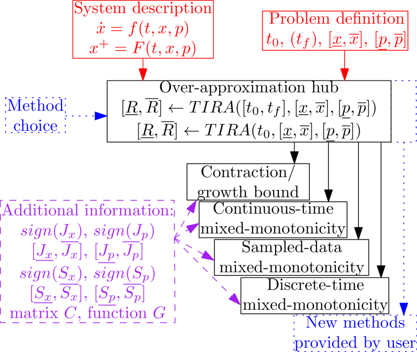
Figure 1. TIRA’s architecture: black blocks are fully implemented in TIRA; colored blocks are possible user inputs implemented as functions to be filled (required in plain red, recommended in dashed purple, optional in dotted blue).

5. Numerical examples

We consider a $n_{x}$-link traffic network describing a diverge junction (the vehicles in link $1$ divide evenly among the outgoing links $2$ and $3$) followed by downstream links so that traffic on link $2$ flows to link $4$ then to link $6$, etc., and, likewise, traffic flows from link $3$ to $5$ to $7$, etc. Let functions $k:\mathbb{R}^{n_{x}}\rightarrow\mathbb{R}$ and $l:\mathbb{R}^{2}\rightarrow\mathbb{R}$ be such that $k(x)=\min(c,vx_{1},2w(\bar{x}-x_{2}),2w(\bar{x}-x_{3}))$ and $l(x_{i},x_{j})=\min\left(c,vx_{i},w(\bar{x}-x_{j})/\beta\right)$. The considered continuous-time model inspired by (Coogan and Arcak, [n. d.]) and written $\dot{x}=f(x)+p$ as in (3) is then given by:

$$f_{1}(x) =-k(x)/T,$$

$$f_{i}(x) =(k(x)/2-l(x_{i},x_{i+2}))/T,\ i\in\{2,3\}$$

$$f_{i}(x) =(\beta l(x_{i-2},x_{i})-l(x_{i},x_{i+2}))/T,\ i\in\{4,\ldots,n\}$$

where the term $w(\bar{x}-x_{i+2})/\beta$ is excluded from the minimization in $l$ for $i\in\{n_{x}-1,n_{x}\}$. State $x\in\mathbb{R}^{n_{x}}$ is the vehicle density on each link, input $p\in\mathbb{R}^{n_{x}}$ is such that $p_{1}\in[4/3,2]$ is the constant but uncertain vehicle inflow to link $1$ and $p_{i}=0$ for $i\geq 2$, and the known parameters of the network $T=30$, $c=40$, $v=0.5$, $\bar{x}=320$, $w=1/6$ and $\beta=3/4$ are taken from (Coogan and Arcak, [n. d.]). Based on these dynamics, we provided to TIRA global bounds for the Jacobian matrices (omitted in this paper due to space limitation).

For the purpose of visualization of the results, we first consider $n_{x}=3$ and run a function trying all the main over-approximation methods implemented in TIRA with an interval of initial states defined by $\underline{x}=[150;180;100]$ and $\overline{x}=[200;300;220]$. The methods based on contraction/growth bound, continuous-time mixed-monotonicity and sampled-data mixed-monotonicity (with both interval arithmetic and sampling/falsification submethods to obtain bounds of the sensitivities matrices) are then successfully run with computation times as reported in Table 1. The method in Section 3.4 is skipped since we do not have a discrete-time system. The projection onto the $(x_{1},x_{2})$-plane of the four over-approximations is showed in Figure 2 alongside an approximation of the actual reachable set by the black cloud of $1000$ sample successor states.

To compare these results with another set representation, we applied the zonotope-based method from CORA (Althoff, 2015) to the same reachability problem with a similar $3$-link network (taking the smooth approximation $\min(a,b)\approx-\log(e^{-a}+e^{-b})$ since the $\min$ operator cannot be used in CORA’s symbolic implementation). CORA solves the reachability problem by decomposing it into a sequence of intermediate reachability analysis between $t_{0}=0$ and $t_{f}=30$s. At each step, CORA linearizes the nonlinear dynamics and if the considered set is too large, it is iteratively split to keep a low linearization error. For these reasons and due to our large interval of initial states, CORA was unable to go further than the time instant $18.3$s after $5$ hours of computation . It is plausible that the performance of CORA in this example could be improved with the choice of the internal solver parameters or by avoiding the use of the smoothed version of $\min$ . TIRA, on the other hand, requires little to no parameter tuning from the user and it does not need the dynamics to be continuously differentiable.

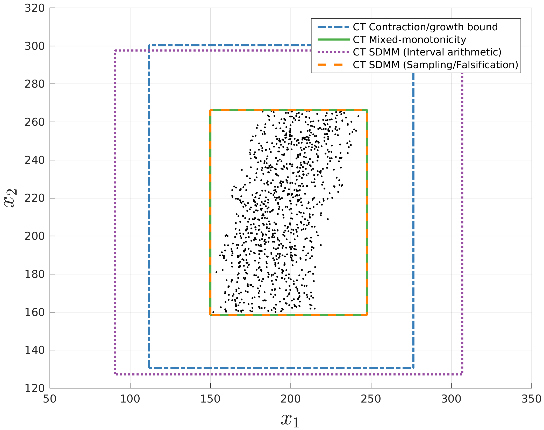
Figure 2. Comparison of four over-approximations for the continuous-time model of a $3$-link traffic network representing a diverge junction (colored intervals) with an approximation of its reachable set (black cloud of sample successors).

To evaluate the scalability of the over-approximation methods, we now consider the $n_{x}$-link network with $n_{x}=99$ and interval of initial states $[\underline{x},\overline{x}]=[100,200]^{n_{x}}$. The sampling and falsification submethod for sampled-data mixed-monotonicity in Section 3.3 is discarded from this test since it does not scale to this dimension because the number of samples should grow exponentially with $n_{x}$ to obtain a decent estimation of the sensitivity bounds. The computation times for the other three methods are given in Table 1. Although the sampled-data mixed-monotonicity approach (with interval arithmetic submethod) appears to have a much worse scalability than the other two, it should be noted that most of its computation time corresponds to the interval arithmetic evaluating the Taylor series of a $n_{x}\times n_{x}$ interval matrix exponential ($332$ seconds), while the reachable set over-approximation itself (as in Proposition 9) only takes $5.4$ seconds.

$n_{x}$	C/GB	MM	SDMM (IA)	SDMM (S/F)	CORA
$3$	$0.13$	$0.050$	$0.28$	$7.0$	($>18000$)
$99$	$0.37$	$4.4$	$338$	-	-

Table 1. Computation times (in seconds) for the over-approximation methods with $n_{x}=3$ and $n_{x}=99$, on a laptop with a $1.7$GHz CPU and $4$GB of RAM.

6. Conclusions and future work

In this paper, we introduced TIRA, a tool library gathering several methods to over-approximate the reachable set of continuous- and discrete-time systems by a multi-dimensional interval. Compared to other tools and reachability approaches primarily aimed at the accuracy of over-approximations, TIRA shifts the focus towards the simplicity and scalability of interval methods, some of which providing tight interval over-approximations. The main feature of TIRA’s architecture is to be easily extensible by users who can add their own interval-based reachability methods.

The main directions for future development of TIRA include exploring interval reachability methods for hybrid systems and using existing interval arithmetic tools (see e.g., IBEX (Chabert and Jaulin, 2009)) to compute Jacobian bounds automatically without requiring user inputs. Comparing the performances of TIRA to other interval-based tools such as DynIBEX (dit Sandretto and Chapoutot, 2016) and VNODE-LP (Nedialkov, 2006) will also be considered.

Appendix A Continuous-time monotonicity

This section presents an over-approximation method which is only applicable to systems satisfying a monotonicity property defined below. While this method is also available in TIRA, it is not presented in Section 3 of this paper because the continuous-time mixed-monotonicity approach in Section 3.2 encompasses it as a particular case. Further comments on the comparison of these two methods are provided at the end of this section.

Requirements and limitations

The monotonicity property for continuous-time systems with inputs (1) is defined in (Angeli and Sontag, 2003) and used for reachability analysis in (Moor and Raisch, 2002). A system (1) is monotone if its Jacobian matrices $J_{x}(t,x,p)$ and $J_{p}(t,x,p)$ are sign-stable (apart from the diagonal of $J_{x}$) over the considered ranges of time, state and input and the sign structure satisfies the following assumption.

Assumption 12.

Given an invariant state space $X\subseteq\mathbb{R}^{n_{x}}$, there exist $\varepsilon=[\varepsilon_{1};\dots;\varepsilon_{n_{x}}]\in\{0,1\}^{n_{x}}$ and $\delta=[\delta_{1};\dots;\delta_{n_{p}}]\in\{0,1\}^{n_{p}}$ such that for all $t\in[t_{0},t_{f}]$, $x\in X$, $p\in[\underline{p},\overline{p}]$, $i,j\in\{1,\dots,n_{x}\}$, $j\neq i$ and $k\in\{1,\dots,n_{p}\}$ we have:

$$(-1)^{\varepsilon_{i}+\varepsilon_{j}}\frac{\partial f_{i}(t,x,p)}{x_{j}}\geq 0,\qquad(-1)^{\varepsilon_{i}+\delta_{k}}\frac{\partial f_{i}(t,x,p)}{p_{k}}\geq 0.$$

Note that the user does not need to know in advance whether their system is monotone since TIRA automatically checks this sign structure by translating Assumption 12 into a system of boolean equations and solving it in the 2-element Galois Field GF(2).

Method description

An over-approximation of the reachable set is computed by evaluating the successor states of (1) for only two pairs $(x,p)\in[\underline{x},\overline{x}]\times[\underline{p},\overline{p}]$ picked based on the boolean vectors $\varepsilon=[\varepsilon_{1};\dots;\varepsilon_{n_{x}}]$ and $\delta=[\delta_{1};\dots;\delta_{n_{p}}]$ satisfying Assumption 12.

Proposition 13.

Under Assumption 12, an over-approximation of the reachable set of (1) in Problem 1 is given by (using componentwise multiplications with $\varepsilon$ and $\delta$):

$$R(t_{f};t_{0},[\underline{x},\overline{x}],[\underline{p},\overline{p}])\subseteq\\ [\Phi(t_{f};t_{0},\underline{x}(1_{n_{x}}-\varepsilon)+\overline{x}\varepsilon,\underline{p}(1_{n_{p}}-\delta)+\overline{p}\delta),\\ \Phi(t_{f};t_{0},\underline{x}\varepsilon+\overline{x}(1_{n_{x}}-\varepsilon),\underline{p}\delta+\overline{p}(1_{n_{p}}-\delta))].$$

Remarks

While Assumption 12 is quite restrictive, whenever it is satisfied the resulting interval in Proposition 13 is guaranteed to be a tight over-approximation of the reachable set. As mentioned in Proposition 7 and proved below in Appendix B.2, applying the continuous-time mixed-monotonicity approach in Proposition 6 to a monotone system satisfying Assumption 12 will result in the same tight interval over-approximation as in Proposition 13. The main differences between these two results is that the monotonicity-specific result in Proposition 13 has a constant complexity (we always only evaluate $\Phi$ for two state-input pairs in $[\underline{x},\overline{x}]\times[\underline{p},\overline{p}]$), while the complexity of the more general result in Proposition 6 is linear in the state dimension $n_{x}$ ($2n_{x}$ evaluations of $\Phi$ are required). On the other hand, Proposition 6 does not need to know whether Assumption 12 is satisfied to obtain this result, while Proposition 13 first requires checking Assumption 12 through the provided function in TIRA which can be time consuming for large systems.

Appendix B Proofs of Section 3.2

In this section, $\mathbb{R}_{+}$ and $\mathbb{R}_{-}$ are the sets of non-negative and non-positive real numbers, respectively.

B.1. Proposition 6

Proof of Proposition 6.

From the definitions of functions $g$ and $h$ in (5)-(7), we have for all $i,j\in\{1,\dots,n_{x}\}$, $j\neq i$ and $k\in\{1,\dots,n_{p}\}$:

$$\frac{\partial h_{i}(t,x,p,\hat{x},\hat{p})}{\partial x_{j}}=\frac{\partial f_{i}(t,\xi^{i},\pi^{i})}{\partial x_{j}}+\alpha^{i}_{j}\geq 0$$

$$\frac{\partial h_{i}(t,x,p,\hat{x},\hat{p})}{\partial\hat{x}_{j}}=\frac{\partial f_{i}(t,\xi^{i},\pi^{i})}{\partial\hat{x}_{j}}-\alpha^{i}_{j}\leq 0$$

$$\frac{\partial h_{i}(t,x,p,\hat{x},\hat{p})}{\partial\hat{x}_{i}}=\frac{\partial f_{i}(t,\xi^{i},\pi^{i})}{\partial\hat{x}_{i}}-\alpha^{i}_{i}=0$$

Similarly, we obtain $\frac{\partial h_{n_{x}+i}}{\partial x_{i}}=0$, $\frac{\partial h_{n_{x}+i}}{\partial x_{j}}\leq 0$, $\frac{\partial h_{n_{x}+i}}{\partial\hat{x}_{j}}\geq 0$, $\frac{\partial h_{i}}{\partial p_{k}}\geq 0$, $\frac{\partial h_{i}}{\partial\hat{p}_{k}}\leq 0$, $\frac{\partial h_{n_{x}+i}}{\partial p_{k}}\leq 0$ and $\frac{\partial h_{n_{x}+i}}{\partial\hat{p}_{k}}\geq 0$. This implies that system (7) is monotone with respect to the orthants $\mathbb{R}^{n_{x}}_{+}\times\mathbb{R}^{n_{x}}_{-}$ and $\mathbb{R}^{n_{p}}_{+}\times\mathbb{R}^{n_{p}}_{-}$. Then from (Angeli and Sontag, 2003), for all $x\in[\underline{x},\overline{x}]$ and $\mathbf{p}:[t_{0},t_{f}]\rightarrow[\underline{p},\overline{p}]$, we have

$$\Phi^{h}(t_{f};t_{0},\underline{x},\underline{p},\overline{x},\overline{p})\preceq_{x}\Phi^{h}(t_{f};t_{0},x,\mathbf{p},x,\mathbf{p})\preceq_{x}\Phi^{h}(t_{f};t_{0},\overline{x},\overline{p},\underline{x},\underline{p})$$

where $\preceq_{x}$ is the partial order defined by the orthant $\mathbb{R}^{n_{x}}_{+}\times\mathbb{R}^{n_{x}}_{-}$, (i.e. for all $x,\hat{x},y,\hat{y}\in\mathbb{R}^{n_{x}}$, $\begin{pmatrix}x\\ \hat{x}\end{pmatrix}\preceq_{x}\begin{pmatrix}y\\ \hat{y}\end{pmatrix}\Leftrightarrow\begin{cases}x\leq y,\\ \hat{x}\geq\hat{y},\end{cases}$ where $\leq$ and $\geq$ are the componentwise inequalities on $\mathbb{R}^{n_{x}}$). From (5), $f$ is embedded in the diagonal of $g$ (i.e. $g(t,x,p,x,p)=f(t,x,p)$), which implies that $\Phi^{h}(t_{f};t_{0},x,\mathbf{p},x,\mathbf{p})=\begin{pmatrix}\Phi(t_{f};t_{0},x,\mathbf{p})\\ \Phi(t_{f};t_{0},x,\mathbf{p})\end{pmatrix}$. Finally, the symmetry of system (7) implies that $\Phi^{h}_{n_{x}+1\dots 2n_{x}}(t_{f};t_{0},\overline{x},\overline{p},\underline{x},\underline{p})=\Phi^{h}_{1\dots n_{x}}(t_{f};t_{0},\underline{x},\underline{p},\overline{x},\overline{p})$, which results in the proposition statement. ∎

B.2. Proposition 7

Proof of Proposition 7.

We start from a system (1) satisfying the monotonicity condition in Assumption 12. Without loss of generality, we assume that the states in $x\in\mathbb{R}^{n_{x}}$ are ordered as $x=[x^{+};x^{-}]$ with $x^{+}\in\mathbb{R}^{n_{x}^{+}}$, $x^{-}\in\mathbb{R}^{n_{x}^{-}}$, $n_{x}^{+}+n_{x}^{-}=n_{x}$ and such that $\varepsilon=[0_{n_{x}^{+}};1_{n_{x}^{-}}]$. We use similar notations $p^{+}\in\mathbb{R}^{n_{p}^{+}}$, $p^{-}\in\mathbb{R}^{n_{p}^{-}}$ and $\delta=[0_{n_{p}^{+}};1_{n_{p}^{-}}]$ for the input vector $p\in\mathbb{R}^{n_{p}}$. We similarly introduce $f^{+}$, $f^{-}$, $\Phi^{+}$, $\Phi^{-}$ for the decomposition of the vector field $f$ and trajectory function $\Phi$ respectively, into their $n_{x}^{+}$ first and $n_{x}^{-}$ last components.

If we now apply the result in Proposition 6 to this monotone system, then for all $i\in\{1,\dots,n_{x}\}$ we have $\alpha^{i}=0_{n_{x}}$, $\beta^{i}=0_{n_{p}}$ and

$$(\xi^{i},\pi^{i})=\begin{cases}(x(1_{n_{x}}-\varepsilon)+\hat{x}\varepsilon,p(1_{n_{p}}-\delta)+\hat{p}\delta)\text{ if }\varepsilon_{i}=0,\\ (x\varepsilon+\hat{x}(1_{n_{x}}-\varepsilon),p\delta+\hat{p}(1_{n_{p}}-\delta))\text{ if }\varepsilon_{i}=1,\end{cases}\\$$

using componentwise multiplications. As a result, system (7) becomes:

(9) $$\begin{pmatrix}\dot{x}^{+}\\ \dot{x}^{-}\\ \dot{\hat{x}}^{+}\\ \dot{\hat{x}}^{-}\end{pmatrix}=h(t,x,p,\hat{x},\hat{p})=\begin{pmatrix}f^{+}(t,[x^{+};\hat{x}^{-}],[p^{+};\hat{p}^{-}])\\ f^{-}(t,[\hat{x}^{+};x^{-}],[\hat{p}^{+};p^{-}])\\ f^{+}(t,[\hat{x}^{+};x^{-}],[\hat{p}^{+};p^{-}])\\ f^{-}(t,[x^{+};\hat{x}^{-}],[p^{+};\hat{p}^{-}])\end{pmatrix}.$$

Since (9) actually contains two decoupled copies of system (1):

$$\begin{pmatrix}\dot{x}^{+}\\ \dot{\hat{x}}^{-}\end{pmatrix}=f(t,[x^{+};\hat{x}^{-}],[p^{+};\hat{p}^{-}]),\quad\begin{pmatrix}\dot{\hat{x}}^{+}\\ \dot{x}^{-}\end{pmatrix}=f(t,[\hat{x}^{+};x^{-}],[\hat{p}^{+};p^{-}]),$$

it implies that any successor of (9) can be expressed as two successors of (1). In particular, for the quadruple of initial states and inputs $(\underline{x},\underline{p},\overline{x},\overline{p})$ used in Proposition 6, we have:

$$\Phi^{h}(t_{f};t_{0},\underline{x},\underline{p},\overline{x},\overline{p})=\begin{pmatrix}\Phi^{+}(t_{f};t_{0},[\underline{x}^{+};\overline{x}^{-}],[\underline{p}^{+};\overline{p}^{-}])\\ \Phi^{-}(t_{f};t_{0},[\overline{x}^{+};\underline{x}^{-}],[\overline{p}^{+};\underline{p}^{-}])\\ \Phi^{+}(t_{f};t_{0},[\overline{x}^{+};\underline{x}^{-}],[\overline{p}^{+};\underline{p}^{-}])\\ \Phi^{-}(t_{f};t_{0},[\underline{x}^{+};\overline{x}^{-}],[\underline{p}^{+};\overline{p}^{-}])\end{pmatrix}.$$

Since $\begin{pmatrix}\underline{x}^{+}\\ \overline{x}^{-}\end{pmatrix},\begin{pmatrix}\overline{x}^{+}\\ \underline{x}^{-}\end{pmatrix}\in[\underline{x},\overline{x}]$ and $\begin{pmatrix}\underline{p}^{+}\\ \overline{p}^{-}\end{pmatrix},\begin{pmatrix}\overline{p}^{+}\\ \underline{p}^{-}\end{pmatrix}\in[\underline{p},\overline{p}]$, we know that $\Phi(t_{f};t_{0},[\underline{x}^{+};\overline{x}^{-}],[\underline{p}^{+};\overline{p}^{-}])$ and $\Phi(t_{f};t_{0},[\overline{x}^{+};\underline{x}^{-}],[\overline{p}^{+};\underline{p}^{-}])$ belong to the actual reachable set $R(t_{f};t_{0},[\underline{x},\overline{x}],[\underline{p},\overline{p}])$ of (1). As a result, the interval defined from the $2n_{x}$ components of $\Phi^{h}(t_{f};t_{0},\underline{x},\underline{p},\overline{x},\overline{p})$ in Proposition 6 is necessarily a tight interval over-approximation of the reachable set.

Since a tight interval over-approximation of a set is uniquely defined and the reachability method defined for monotone systems in Proposition 13 is also known to provide a tight interval over-approximation of the reachable set, we can conclude that both methods provide the same results. ∎

References

- (1)
- Althoff (2015) Matthias Althoff. 2015. An Introduction to CORA 2015. In ARCH@ CPSWeek. 120–151.
- Althoff et al. (2007) Matthias Althoff, Olaf Stursberg, and Martin Buss. 2007. Reachability analysis of linear systems with uncertain parameters and inputs. In 46th IEEE Conference on Decision and Control. IEEE, 726–732.
- Angeli and Sontag (2003) David Angeli and Eduardo D. Sontag. 2003. Monotone Control Systems. IEEE Trans. Automat. Control 48, 10 (2003), 1684–1698.
- Arcak and Maidens (2018) M. Arcak and J. Maidens. 2018. Simulation-based reachability analysis for nonlinear systems using componentwise contraction properties. In Principles of Modeling, M. Lohstroh, P. Derler, and M. Sirjani (Eds.). Springer, 61–76.
- Chabert and Jaulin (2009) Gilles Chabert and Luc Jaulin. 2009. Contractor programming. Artificial Intelligence 173 (2009), 1079–1100.
- Chen et al. (2013) Xin Chen, Erika Ábrahám, and Sriram Sankaranarayanan. 2013. Flow*: An analyzer for non-linear hybrid systems. In International Conference on Computer Aided Verification. Springer, 258–263.
- Chu and Huang (1998) Tianguang Chu and Lin Huang. 1998. Mixed monotone decomposition of dynamical systems with application. Chinese science bulletin 43, 14 (1998), 1171–1175.
- Coogan and Arcak ([n. d.]) Samuel Coogan and Murat Arcak. [n. d.]. A Benchmark Problem in Transportation Networks. arXiv preprint arXiv:1803.00367 ([n. d.]).
- Coogan and Arcak (2015) Samuel Coogan and Murat Arcak. 2015. Efficient finite abstraction of mixed monotone systems. In 18th International Conference on Hybrid Systems: Computation and Control. ACM, 58–67.
- Coogan et al. (2016) Samuel Coogan, Murat Arcak, and Alexander A. Kurzhanskiy. 2016. Mixed monotonicity of partial first-in-first-out traffic flow models. In 55th IEEE Conference on Decision and Control. IEEE, 7611–7616.
- dit Sandretto and Chapoutot (2016) Julien Alexandre dit Sandretto and Alexandre Chapoutot. 2016. Validated Explicit and Implicit Runge–Kutta Methods. Reliable Computing 22, 1 (Jul 2016), 79–103.
- Dreossi (2017) Tommaso Dreossi. 2017. Sapo: reachability computation and parameter synthesis of polynomial dynamical systems. In 20th International Conference on Hybrid Systems: Computation and Control. ACM, 29–34.
- Frehse et al. (2011) Goran Frehse, Colas Le Guernic, Alexandre Donzé, Scott Cotton, Rajarshi Ray, Olivier Lebeltel, Rodolfo Ripado, Antoine Girard, Thao Dang, and Oded Maler. 2011. SpaceEx: Scalable verification of hybrid systems. In International Conference on Computer Aided Verification. Springer, 379–395.
- Hirsch and Smith (2005) Morris W. Hirsch and Hal Smith. 2005. Monotone maps: a review. Journal of Difference Equations and Applications 11, 4-5 (2005), 379–398.
- Jaulin et al. (2001) Luc Jaulin, Michel Kieffer, Olivier Didrit, and Eric Walter. 2001. Applied interval analysis: with examples in parameter and state estimation, robust control and robotics. Vol. 1. Springer Science & Business Media.
- Kapela and Zgliczyński (2009) Tomasz Kapela and Piotr Zgliczyński. 2009. A Lohner-type algorithm for control systems and ordinary differential inclusions. Discrete and Continuous Dynamical Systems. Series B 11, 2 (2009), 365–385.
- Kurzhanskiy and Varaiya (2006) Alex A. Kurzhanskiy and Pravin Varaiya. 2006. Ellipsoidal toolbox (ET). In 45th IEEE Conference on Decision and Control. IEEE, 1498–1503.
- Mazo Jr et al. (2010) Manuel Mazo Jr, Anna Davitian, and Paulo Tabuada. 2010. PESSOA: A tool for embedded controller synthesis.. In International Conference on Computer Aided Verification. Springer, 566–569.
- Meyer et al. (2018) Pierre-Jean Meyer, Samuel Coogan, and Murat Arcak. 2018. Sampled-data reachability analysis using sensitivity and mixed-monotonicity. IEEE Control Systems Letters 2, 4 (2018), 761–766.
- Meyer and Dimarogonas (2018) Pierre-Jean Meyer and Dimos V. Dimarogonas. 2018. Hierarchical decomposition of LTL synthesis problem for nonlinear control systems. arXiv preprint arXiv:1712.06014 (2018).
- Mitchell and Templeton (2005) Ian M. Mitchell and Jeremy A. Templeton. 2005. A toolbox of Hamilton-Jacobi solvers for analysis of nondeterministic continuous and hybrid systems. In International Workshop on Hybrid Systems: Computation and Control. Springer, 480–494.
- Moor and Raisch (2002) Thomas Moor and Jörg Raisch. 2002. Abstraction based supervisory controller synthesis for high order monotone continuous systems. In Modelling, Analysis, and Design of Hybrid Systems. Springer, 247–265.
- Nedialkov (2006) Ned Nedialkov. 2006. VNODE-LP. Technical Report CAS-06-06-NN. Dept. of Computing and Software, McMaster Univ. Hamilton, ON, Canada.
- Reissig et al. (2016) Gunther Reissig, Alexander Weber, and Matthias Rungger. 2016. Feedback refinement relations for the synthesis of symbolic controllers. IEEE Trans. Automat. Control 62, 4 (2016), 1781–1796.
- Rungger and Zamani (2016) Matthias Rungger and Majid Zamani. 2016. SCOTS: A tool for the synthesis of symbolic controllers. In Proceedings of the 19th International Conference on Hybrid Systems: Computation and Control. ACM, 99–104.
- Xue et al. (2017) Bai Xue, Martin Fränzle, and Peter Nazier Mosaad. 2017. Just Scratching the Surface: Partial Exploration of Initial Values in Reach-Set Computation. In 56th IEEE Conference on Decision and Control. 1769–1775.
- Yang et al. (2018) Liren Yang, Oscar Mickelin, and Necmiye Ozay. 2018. On sufficient conditions for mixed monotonicity. arXiv preprint arXiv:1803.04528 (2018).