Estimation of Gaussian directed acyclic graphs using partial ordering information with an application to dairy cattle data

Abstract

Estimating a directed acyclic graph (DAG) from observational data represents a canonical learning problem and has generated a lot of interest in recent years. Research has focused mostly on the following two cases: when no information regarding the ordering of the nodes in the DAG is available, and when a domain-specific complete ordering of the nodes is available. In this paper, motivated by a recent application in dairy science, we develop a method for DAG estimation for the middle scenario, where partition based partial ordering of the nodes is known based on domain-specific knowledge. We develop an efficient algorithm that solves the posited problem, coined Partition-DAG. Through extensive simulations using the DREAM3 Yeast data, we illustrate that Partition-DAG effectively incorporates the partial ordering information to improve both speed and accuracy. We then illustrate the usefulness of Partition-DAG by applying it to recently collected dairy cattle data, and inferring relationships between various variables involved in dairy agroecosystems.

secReferenceswss

, , , , and

1 Introduction

The problem of estimating a directed acyclic graph (DAG) from high-dimensional observational data has attracted a lot of attention recently in the statistics and machine learning literature, due to its importance in a number of application areas including molecular biology. In the latter area, high throughput techniques have enabled biomedical researchers to profile biomolecular data to better understand causal molecular mechanisms involved in gene regulation and protein signaling (Emmert-Streib et al. (2014)). Further, it provided the impetus for the develoment of numerous approaches for tackling the problem - see for example the review paper Marbach et al. (2012) and references therein.

This is a challenging learning problem in its general form. It stems from the fact that in order to reconstruct a DAG from data, one has to consider all possible orderings of nodes and score the resulting network structures based on evidence gleaned from the available data. The computational complexity of obtaining all possible orderings of a set of nodes in a directed graph is exponential in the size of the graph. In certain applications, one may have access to a complete topological ordering, which renders the problem computationally tractable as discussed below. An interesting question arises of what advantages, the availability of external information on partial orderings of nodes, brings to solving the problem. This is the key issue addressed in this study, motivated by an application on dairy operations, where such information can be reliably obtained from operators as explained next.

Dairy cattle operations are characterized by complex interactions between several factors which determine the success of these systems. Most of these operationsresult in the collection of large amounts of data that are usually analyzed using univariate statistical models for certain variables of interest; therefore, information from relationships between these variables is ignored. In addition, due to the structure of a dairy cattle agroecosystem, it is of great interest to carry out data analysis that permits to implement a systemic approach (Jalvingh (1992); Thornley and France (2007)). Moreover, due to their high relevance when making management decisions and recommendations, knowing not only interaction patterns, but also causal relationships between the components of dairy production systems, is a problem of current interest, and has the potential to have a marked impact on the dairy industry. In any of these systems (such as the data analyzed in Section 4), causal relationships between selected pairs of variables are reliably known. The statistical task then, is to leverage these known relationships and the observed data to estimate the underlying network of relationships between the variables under consideration.

In particular, suppose ${\bf Y}_{1},...,{\bf Y}_{n}\in\mathbb{R}^{p}$ are i.i.d. random vectors from a multivariate distribution with mean ${\bf 0}$ and covariance matrix $\Sigma=\Omega^{-1}$. In sample deprived settings, an effective and popular method for estimating $\Sigma$ imposes sparsity on the entries of $\Sigma$ (covariance graph models), or $\Omega$ (graphical models), or appropriate Cholesky factors of $\Omega$ (directed acyclic graph models or Bayesian networks). The choice of an appropriate model often depends on the application.

In this study, our focus is on learning DAG from high-dimensional data, assuming sparsity in an appropriate Cholesky factor of $\Omega$. In particular, consider the factorization of the inverse covariance matrix $\Omega=B^{t}B$, where $B$ can be converted to a lower triangular matrix with positive diagonal entries through a permutation of rows and columns. The sparsity pattern of $B$ gives us a directed acyclic graph (DAG), which is defined as $G=(V,E)$ where $V=\{1,...,p\}$ and $E=\{i\to j:B_{ij}\neq 0\}$. The assumption $B_{ij}=0$ corresponds to assuming an appropriate conditional independence under Gaussianity, and corresponds to assuming an appropriate conditional correlation being zero in the general setting.

There are two main lines of work that have dealt with DAG estimation in the Gaussian framework - one where the permutation that makes B lower triangular is known and one where it is unknown. We brifely discuss them below. As previously mentioned, nn many applications, a natural ordering, such as time based or location based ordering, of the variables presents itself, and hence a natural choice for the permutation which makes $B$ lower triangular is available. Penalized likelihood methods, which use versions of the $\ell_{1}$ penalty, and minimize the respective objective functions over the space of lower triangular matrices, have been developed in Huang et al. (2006); Shojaie and Michailidis (2010); Khare et al. (2017). Bayesian methods for this setting have been developed in Cao et al. (2017); Altamore et al. (2013); Consonni et al. (2017). For many of these methods, high dimensional consistency results for the model parameters have also been established.

If the permutation/ordering that makes $B$ lower triangular is unknown, then the problem becomes significantly more challenging, both computationally and theortically. In this setting, several score- based, constraint-based and hybrid algorithms for estimating the underlying CPDAG  have been developed and studied in the literature (Spirtes et al. (2001); Geiger and Heckerman (2013); Lam and Bacchus (1994); Heckerman et al. (1995); Chickering (2003); Ellis and Wong (2008); Zhou (2011); Kalisch and B¨uhlmann (2007); Tsamardinos et al. (2006); Gamez et al. (2011, 2012); van de Geer and Buhlmann (2013)). See Aragam and Zhou (2015) for an excellent and detailed review. Recently, Aragam and Zhou (2015) have developed a penalized likelihood approach called CCDr for sparse estimation of $B$, which has been shown to be significantly more computationally scalable than previous approaches.

However, in some applications, such as the dairy cattle data studied in Section 4, domain-specific information regarding the variables in available, which allows for a partition of the variables into sets $V_{1},V_{2},\cdots,V_{k}$ such that any possible edge from a vertex in $V_{i}$ to a vertex in $V_{j}$ is directed from $v_{i}$ to $v_{j}$ if $i<j$. However, the ordering of the variables in the same subset is not known, and has to be inferred from the data. This setting is not subsumed in the previous approaches mentioned above, and falls somewhere in the middle of the two extremes of having complete information regarding the ordering, and having no information regarding the ordering. The goal of this paper is to develop a hybrid approach for DAG estimation which leverages the partition based partial ordering information. We will also show that using the partition information leads to a reduction in the number of computations, and more importantly allows for parallel processing, unlike CCDr. This can lead to significant improvement in computational speed and statistical performance.

The remainder of the paper is organized as follows. In Section 2, we develop, and describe in detail, our hybrid algorithm called Partition-DAG. In Section 3, we perform a detailed experimental study to evaluate and understand the performance of the proposed algorithm. In Sections 3.1, 3.2 and 3.3, we use known DAGs from the DREAM3 competition (Prill et al. (2010); Marbach et al. (2010, 2009)) and perform an extensive simulation study to explore the effectiveness/ability of Partition-DAG to incorporate the ordering information, and how this ability changes with more/less informative partitions. In Section 3.4, we perform a similar simulation study, this time using randomly generated DAGs with more number of variables. Finally, in Section 4 we analyze dairy cattle data recently gathered by Universidad Nacional de Colombia using the proposed Partition-DAG approach.

2 DAG estimation using partition information and the corresponding Partition-DAG algorithm

In order to understand how one can leverage the partial ordering information, it is crucial to understand the workings, similarities, and differences of the Concave penalized Coordinate Descent with reparameterization (CCDr) Aragam and Zhou (2015) and the Convex Sparse Cholesky Selection (CSCS) Khare et al. (2017) algorithms, which are state of the art in terms on computational scalability and convergence for the boundary settings with completely unknown and completely known variable ordering respectively.

The CSCS algorithm is derived under the setting where a domain-specific ordering of the variables which makes $B$ lower triangular is known. Hence, the DAG estimation problem boils down to estimating the sparsity pattern in $L$, the lower triangular permuted version of $B$. In other words, $L$ is a lower triangular matrix with positive diagonal entries such that $\Omega=L^{t}L$. The objective function for CSCS is

$$Q_{cscs}(L) =\operatorname*{trace}(\Omega S)-\frac{1}{2}\log\left|\Omega\right|+\lambda\sum_{1\leq j<i\leq p}\left|L_{ij}\right|$$

$$=\operatorname*{trace}(L^{t}LS)-\log\left|L\right|+\lambda\sum_{1\leq j<i\leq p}\left|L_{ij}\right|,$$

where $S$ is the sample covariance matrix. The first two terms in $Q_{cscs}$ correspond to the Gaussian log-likelihood, and the third term is an $\ell_{1}$ penalty term which induces sparsity in the lower triangular matrix $L$.

The CCDr algorithm is derived under the setting where there is no knowledge about the permutation that makes $B$ lower triangular. Here $\Omega=B^{t}B$, where $B$ varies over the space of $p\times p$ matrices such that by permuting the rows and columns of $B$ we can reduce it to a lower triangular matrix with positive diagonal entries. More formally, denoting $S_{p}$ to be the group of permutations of $\{1,2,\cdots,p\}$, we assume that $B\in\mathcal{B}_{p}$, where

$$\mathcal{B}_{p}=\{B:\exists\sigma\in S_{p}\mbox{ such that }B_{\sigma(i)\sigma(j)}=0\mbox{ if }i<j\}.$$

The CCDr-$\ell_{1}$ method uses the following objective function:

$$Q_{CCDr}(B) =\operatorname*{trace}(\Omega S)-\frac{1}{2}\log\left|\Omega\right|+\lambda\sum_{1\leq i\neq j\leq p}\left|B_{ij}\right|$$

$$=\operatorname*{trace}(B^{t}BS)-\frac{1}{2}\log\left|B^{t}B\right|+\lambda\sum_{1\leq i\neq j\leq p}\left|B_{ij}\right|$$

Exactly like CSCS the first two terms correspond to the Gaussian log-likelihood, while the third term tries to impose sparsity on $B$.

While objective functions for CSCS and CCRr-$\ell_{1}$ look identical, the algorithms to minimize the two objective functions are very different due to the fact that we are minimizing over different spaces. Both objective functions are convex, but CSCS has the added advantage that the range for $Q_{cscs}$, which is the set of lower triangular matrices with positive diagonal entries, is convex as well. This leads to a convex problem (though not strictly convex for $n<p$) and we can establish that the sequence of iterates converges to a global minimum of the objective function. However, the range for $Q_{CCDr}(B)$, which is the set of matrices that can be converted to a lower triangular matrix with positive diagonal entries through a permutation of the rows and columns, is not convex and general results in the literature (at best) only guarantee convergence of the sequence of iterates to a local minimum of the objective function. In addition, while CSCS can be broken down into $p$ parallelizable problems the same can not be said for CCDr, which leads to a significant computational disadvantage for CCDr. Finally, asymptotic consistency for the general setting (with no restrictions on conditional variances) for CCDr isn’t available as yet, whereas Theorem 4.1 in Khare et al. (2017) establishes both model selection and estimation consistency for CSCS. See Khare et al. (2017) for a more detailed comparison between these two algorithms.

As stated in the introduction, in many applications, additional data can give information about partitions of the variables where we have prior knowledge about the direction of the edges between partitions, but not within partitions (for example, the dairy cattle data in Section 4, or gene knock-out data or more general perturbations data Shojaie et al. (2014)). We will now discuss how one can create a hybrid algorithm from CSCS and CCDr where we incorporate this information for DAG estimation.

2.1 The case with two partition blocks

For simplicity we will initially work with the case where the variables, $V=\{1,...,p\}$, are divided into two groups $V_{1}=\{1,...,m\}$ and $V_{2}=\{m+1,...,p\}$ such that we cannot have an edge from a node in $V_{2}$ to one in $V_{1}$, but can have one from a node in $V_{1}$ to one in $V_{2}$. Hence, $\forall j\in V_{1},\forall k\in V_{2}$ we have that $B_{kj}=0$. This implies that B has the block triangular form

$$B=\begin{pmatrix}\mathbf{B}_{11}&\mathbf{0}\\ \mathbf{B}_{21}&\mathbf{B}_{22}\\ \end{pmatrix}$$ (2.1)

The diagonal blocks ${\bf B}_{11}$ and ${\bf B}_{22}$ are constrained so that each matrix is a permuted version of lower triangular matrices, i.e., ${\bf B}_{11}\in\mathcal{B}_{m}$ and ${\bf B}_{22}\in\mathcal{B}_{p-m}$, the entries of the off-diagonal block ${\bf B}_{12}$ are all zero. However, there are no constraints on the off-diagonal block ${\bf B}_{21}$. Similar to CCDr, we consider a Gaussian log-likelihood based objective function, denoted by $Q_{PDAG}$, given by

$$Q_{PDAG}({\bf B})=\operatorname*{trace}(\Omega S)-\frac{1}{2}\log\left|\Omega\right|+\lambda\sum_{1\leq i\neq j\leq p}\left|B_{ij}\right|.$$

Here, our goal is to minimize the above function over the space $\widetilde{\mathcal{B}}_{p}$, defined by

$$\widetilde{\mathcal{B}}_{p}=\{{\bf B}:{\bf B}_{11}\in\mathcal{B}_{m},{\bf B}_{22}\in\mathcal{B}_{p-m},{\bf B}_{12}={\bf 0}\},$$

as opposed to CCDr, where the goal is to minimize over the space $\mathcal{B}_{p}$. Note that since $\mathcal{B}_{m}$ and $\mathcal{B}_{p-m}$ are not convex sets, $\widetilde{\mathcal{B}}_{p}$ is also not a convex set.

2.1.1 A roadmap for the algorithm

As in CCDr and CSCS, we pursue a coordinate-wise minimization approach. At each iteration, we cycle through minimizing $Q_{PDAG}$ with respect to each non-trivial element of $B$ (fixing the other entries at their current values). The minimizing value is then set as the new value of the corresponding element. We repeat the iterations until the difference between the $B$ values at two successive iterations falls below a user-defined threshold.

Hence, for implementing coordinate-wise minimization, we need to understand how to minimize $Q_{PDAG}$ with respect to an arbitrary element $B_{ij}$ of ${\bf B}$ given all the other elements. Using straightforward calculations, we get

$$Q_{PDAG}({\bf B})$$

$$=\operatorname*{trace}({\bf B}^{t}{\bf B}S)-\frac{1}{2}\log\left|{\bf B}^{t}{\bf B}\right|+\lambda\sum_{1\leq i\neq j\leq p}\left|B_{ij}\right|$$

$$=\sum_{i=1}^{p}\Big{(}\big{(}\sum_{h=1}^{p}S_{hh}B_{ih}^{2}+2\sum_{k=1}^{p-1}\sum_{l=k+1}^{p}S_{kl}B_{ik}B_{il}\big{)}-\log B_{ii}+\lambda\sum_{j=1,j\neq i}^{p}\left|B_{ij}\right|\Big{)}$$ (2.2)

Given the nature of the constraints on each block of ${\bf B}\in\widetilde{\mathcal{B}}_{p}$, we consider three different cases.

• Case I: (Diagonal entries - $B_{ii}$) It follows from (2.2) that $Q_{PDAG}$ is the sum of quadratic and logarithmic terms in a given diagonal entry $B_{ii}$ (treating other entries as fixed). In particular,

  $$Q_{PDAG}(B_{ii})=S_{ii}B_{ii}^{2}+2B_{ii}\sum_{k=1,k\neq i}^{p}S_{ik}B_{ik}-\log B_{ii}+\mbox{ terms independent of }B_{ii}.$$

  Simple calculus shows that the unique minimizer (with respect to $B_{ii}$) of the above function is given by

  $$\hat{B}_{ii}=\frac{-2\sum_{k=1,k\neq i}^{p}S_{ik}B_{ik}+\sqrt{4(\sum_{k=1,k\neq i}^{p}S_{ik}B_{ik})^{2}+8S_{ii}}}{2S_{ii}}$$ (2.3)

• Case II: (Off-diagonal entries in ${\bf B}_{21}$, the CSCS case) Consider $B_{ij}$, where $m+1\leq i\leq p$ and $1\leq j\leq m$. Since $B_{ji}=0$, it follows from (2.2) that $Q_{PDAG}$ is the sum of quadratic and absolute value terms in $B_{ij}$ (treating other entries as fixed). In particular,

  $$Q_{PDAG}(B_{ij})=S_{jj}B_{ij}^{2}+2B_{ij}\sum_{k=1,k\neq j}^{p}S_{jk}B_{ik}+\lambda\left|B_{ij}\right|+\mbox{ terms independent of }B_{ij}.$$ (2.4)

  Simple calculus shows that the unique minimizer (with respect to $B_{ij}$) of the above function is given by

  $$\hat{B}_{ij}=\mathcal{S}\Big{(}\frac{-\sum_{k=1,k\neq j}^{p}S_{jk}B_{ik}}{2S_{jj}},\frac{\lambda}{4S_{jj}}\Big{)},$$ (2.5)

  where $\mathcal{S}(x,\lambda)=\operatorname*{sign}(x)\max\{\left|x\right|-\lambda,0\}$. This step exactly resembles Case a typical step of the CSCS algorithm.

• Case III: (Off-diagonal entries in ${\bf B}_{11}$ and ${\bf B}_{22}$, the CCDr case) Consider $B_{ij}$, where $1\leq i\neq j\leq m$ or $m+1\leq i\neq j\leq p$. Since ${\bf B}_{11}\in\mathcal{B}_{m}$ and ${\bf B}_{22}\in\mathcal{B}_{p-m}$, it follows that at most one of $B_{ij}$ or $B_{ji}$ is non-zero. So as in CCDr Aragam and Zhou (2015), we will jointly minimize $Q_{PDAG}$ as a function of $(B_{ij},B_{ji})$. This can be done as follows. If adding a non-zero value for $B_{ij}$ violates the DAG constraint, or equivalently the constraint that ${\bf B}_{11}\in\mathcal{B}_{m}$ and ${\bf B}_{22}\in\mathcal{B}_{p-m}$, then we set $B_{ij}=0$, and then minimize $Q_{PDAG}$ as a function of $B_{ji}$ and update the $B_{ji}$ entry as specified in (2.4), (2.5) with the roles of $i$ and $j$ exchanged). If adding a non-zero value for $B_{ji}$ violates the DAG constraint, then we set $B_{ji}=0$, and then minimize $Q_{PDAG}$ as a function of $B_{ij}$ and update the $B_{ij}$ entry as specified in (2.4), (2.5). However, it is possible that neither $\left|B_{ij}\right|>0$ or $\left|B_{ji}\right|>0$ violates the DAG constraint. In that case, we compute $\hat{B}_{ij}$ and $\hat{B}_{ji}$ using appropriate versions of (2.5), pick the one that makes a larger contribution towards minimizing $Q_{PDAG}$, and set the other one to zero. This step exactly resembles a typical step of the CCDr-$\ell_{1}$ algorithm.

The resulting coordinatewise minimization algorithm for $Q_{PDAG}$, called Partition-DAG, which repeatedly iterates through all the entries of ${\bf B}$ based on the three cases discussed above, is provided in Algorithm LABEL:alg:pdag. Case II and Case III, which correspond to typical steps of the CSCS and CCDr algorithm respectively, demonstrate why we regard the Partition-DAG algorithm as a hybrid of these two algorithms.

2.2 The case with multiple partition blocks

Algorithm LABEL:alg:pdag can be easily generalized to the case where the variables are partitioned into $R$ blocks, say, $V_{1},V_{2},\cdots,V_{R}$, such that any edge from a node $u$ in $V_{i}$ to a node $v$ in $V_{j}$ is directed from $u$ to $v$, if $i<j$. However, the ordering within each $V_{i}$ is not known. In particular, let $V_{i}=\{m_{i-1}+1,\cdots,m_{i}\}$, where $m_{0}=0$ and $m_{R}=p$. Under these constraints, the matrix $B$ has a block lower triangular structure, which can be denoted as follows.

$$B=\begin{pmatrix}\mathbf{B}_{11}&\mathbf{0}&\ldots&\mathbf{0}\\ \mathbf{B}_{21}&\mathbf{B}_{22}&\ldots&\mathbf{0}\\ \vdots&\vdots&\ddots&\vdots\\ \mathbf{B}_{R1}&\mathbf{B}_{R2}&\ldots&\mathbf{B}_{RR}\\ \end{pmatrix}$$ (2.6)

In particular, the parameter $B$ lies in the space $\widetilde{\mathcal{B}}_{p,R}$ given by

$$\widetilde{\mathcal{B}}_{p,R}=\{{\bf B}:{\bf B}_{ii}\in\mathcal{B}_{m_{i}-m_{i-1}},\;{\bf B}_{rs}={\bf 0}\mbox{ if }1\leq r<s\leq R\}.$$

We again use a coordinate-wise minimization approach for minimizing $Q_{PDAG}$ over $\widetilde{\mathcal{B}}_{p,R}$. Similar to the two partition block case, the coordinate-wise minimizations can be divided into three cases.

• The first case deals with a diagonal entries $B_{ii}$, and the unique minimizer has exactly the same form as in (2.3).

• The second case (the CSCS case) deals with off-diagonal entries $B_{ij}$ which belong to one of the lower triangular blocks ${\bf B}_{rs}$ with $1\leq s<r\leq R$, and the unique minimizer has exactly the same form as in (2.4).

• Finally, the third case (the CCDr case) deals with off-diagonal entries $B_{ij}$ which belong to one of the diagonal blocks ${\bf B}_{ii}$ with $1\leq r\leq R$, and the unique minimizer has eactly the same form as in (2.5). The algorithm, using the steps described above, is provided as Algorithm LABEL:alg:pdagR in the appendix.

Note that while $Q_{PDAG}$ is jointly convex in $B$, the domain of minimization $\widetilde{\mathcal{B}}_{p,R}$ is not a convex set. Hence, to the best of our knowledge, existing results in the literature do not imply convergence of the coordinate-wise minimization algorithm (Algorithm LABEL:alg:pdagR). Using standard arguments (for example, similar to Theorem 4.1 of Tseng (2001)), the following result can be established.

Lemma 2.1

Assuming that all the diagonal entries of $S$ are positive, any cluster point of the sequence of iterates produced by Algorithm LABEL:alg:pdagR is a stationary point of $Q_{PDAG}$ in $\widetilde{\mathcal{B}}_{p,R}$.

2.3 Advantages of Partition-DAG

We now discuss some of the computational and statistical advantages of using the partition based ordering information in the DAG estimation algorithms derived in this paper.

1. (Parallelizability) Consider the general multiple block case described in Section 2.2. After some manipulations, it can be shown that the objective function $Q_{PDAG}$ can be decomposed as a sum of $R$ functions, where each function exclusively uses entries from a distinct block row of $B$. In particular, it can be shown that

   $$Q_{PDAG}({\bf B})=\sum_{r=1}^{R}Q_{r}({\bf B}_{r1},{\bf B}_{r2},\cdots,{\bf B}_{rr}),$$

   where

   $$Q_{r}({\bf B}_{r1},{\bf B}_{r2},\cdots,{\bf B}_{rr}) =\sum_{i=m_{r-1}+1}^{m_{r}}\Big{(}\big{(}\sum_{h=1}^{m_{r}}S_{hh}B_{ih}^{2}+2\sum_{k=1}^{m_{r}-1}\sum_{l=k+1}^{m_{r}}S_{kl}B_{ik}B_{il}\big{)}$$

   $$-\log B_{ii}+\lambda\sum_{k=1,k\neq i}^{m_{r}}\left|B_{ik}\right|\Big{)}$$

   only depends on the terms in block row $r$. As a result, the minimization of each block row can be implemented in parallel as shown in Algorithm LABEL:alg:pdagR. This can lead to huge computational advantages, as illustrated in our experiments.

2. (Number of computations) With the additional partition information, many of the entries in $B$ are automatically set to zero. This reduces the number of computations Partition-DAG needs to do in comparison to CCDr. In addition, many of the computations we carry out for Partition-DAG fall under Case II as discussed in Section 2.1, which is much simpler and faster than computations under Case III, which is what CCDr needs to do for every single coordinate.

3. (Estimation Accuracy) This is very obvious, but leveraging more information can lead to a improved estimation accuracy as borne out in our simulations studies.

3 Simulation experiments

In this section, we perform extensive simulations using four algorithms: CCDr (no ordering information is assumed to be known), PC algorithm (see Kalisch and Buhlmann (2007), no ordering information is assumed to be known), the proposed Partition-DAG (partial ordering information is assumed to be known), and CSCS (assumes full ordering is known). The goal is to understand/explore the following questions about the Partition-DAG algorithm in realistic settings.

• Can Paritition-DAG effectively leverage the partial ordering information to improve performance (as compared to methods such as CCDr and PC algorithm which do not use any ordering information)?

• As the partitions become finer, does the performance of Partition-DAG improve?

• If the number of sets in the partition is kept the same, but the elements of these sets are changes so that the partition is more informative, then does the performance of Partition-DAG improve?

• How does the computational speed of Partition-DAG compare to CCDr, and how does this change when the partition becomes finer?

We investigate each of these questions separately in the subsections below. The testing based PC algorithm is much slower than the penalized algorithms (CSCS, Partition-DAG, CCDr), but serves as a popular benchmark, and hence is included in the first two subsections below when the number of network nodes is $50$. In Section 3.4, we consider networks with $100$ and $200$ nodes, and the PC algorithm can be very slow in these settings. Hence, we do not include it in Section 3.4.

3.1 Partial ordering info vs. no ordering info: DREAM3 data

The goal of this experiment is to explore if partition based ordering information can help improve accuracy and computational efficiency in realistic settings. With this in mind, we perform a number of simulation studies using gene regulatory networks from the DREAM3 In Silico challenge Prill et al. (2010); Marbach et al. (2010, 2009). This challenge provides the transcriptional networks for three yeast organisms, which we will denote as Yeast 1, Yeast 2, Yeast 3. These networks mimic activations and regulations that occur in gene regulatory networks. All networks are known and have 50 nodes.

For each DAG, we generated a random $B$ by sampling the off-diagonal non-zero terms from a uniform distribution between 0.3 and 0.7 and assigned them a positive or negative sign with equal probability. The diagonal terms were all set to 1. Then, the “true” $\Omega=B^{t}B$ was computed, and the corresponding multivariate Gaussian distribution was used to generate twenty datasets each for sample size $n\in\{40,50,100,200\}$. For each sample size, each of the three algorithms (PC, CCDr, Partition-DAG) was run for each dataset described above for a range of penalty parameter values (for the PC algorithm, the significance level for the hypothesis tests was used as a penalty parameter). Note that the DAG estimation problem is a three way classification problem (two classes corresponding to two kinds of directed edges, and one class corresponding to no edge). Hence, the performance was summarized using the corresponding mean AUC-MA (Macro-averaged Area-Under-the-Curve, see for example Tsoumakas et al. (2010)) value over the twenty repetitions. For each method, the appropriate penalty parameter (or significance level in the case of the PC algorithm) was varied over a range of 30 values to yield a completely sparse network at one end, and a completely dense network (ignoring edge directions) at the other end. The AUC values for the three binary classification problems (corresponding to each class) were then computed and normalized by dividing with the respective false positive rate (FPR) range. The AUC-MA was then computed by taking the average of the three class-wise AUC values. The results for the three different networks (Yeast1, Yeast2, Yeast3) are summarized in Table 1.

As expected, the performance of each method improves with increasing sample size. It is clear that Partition-DAG outperforms both the PC algorithm and the CCDr algorithm for all the DAGs by quite a large margin and the performance is more or less consistent regardless of the complexity of the DAG topology. This demonstrates that the Partition-DAG algorithm can successfully leverage the partial ordering information to improve performance.

Method	Sample size	AUC-MA (Yeast 1)	AUC-MA (Yeast 2)	AUC-MA (Yeast 3)
CCDr	40	0.5097	0.4413	0.4397
Partition-DAG	40	0.6470	0.5842	0.5619
PC	40	0.4743	0.4160	0.4211
CCDr	50	0.5242	0.4505	0.4489
Partition-DAG	50	0.6548	0.6108	0.5767
PC	50	0.5009	0.4273	0.4278
CCDr	100	0.5624	0.4815	0.4716
Partition-DAG	100	0.6830	0.6302	0.6004
PC	100	0.5470	0.4491	0.4576
CCDr	200	0.5884	0.4943	0.4895
Partition-DAG	200	0.7070	0.6544	0.6150
PC	200	0.5795	0.4780	0.4822

Table 1: Macro Averaged Area-Under-the-Curve (AUC-MA) values for Yeast 1, Yeast 2, and Yeast 3 networks for CCDr, Partition-DAG and PC algorithm

3.2 Fine partition vs. coarse partition: Yeast 3 network

Note that given a partition, Partition-DAG assumes the ordering of edges between the sets in the partition to be known, and the ordering of edges within each partition set to be unknown). The goal of this subsection is to explore if using a finer partition (and hence more knowledge of the ordering) improves the performance of the Partition-DAG approach. We perform simulations using the Yeast 3 data from the DREAM3 challenge mentioned in Section 3.1. Recall that the underlying network is known, mimics activations and regulations that occur in gene regulatory networks and has $p=50$ nodes. We topologically order the nodes from $1$ to $50$, so that any edge directs from a smaller node to a bigger node. Again, we construct a “true” $\Omega$ matrix consistent with the known DAG, and generated hundred multivariate datasets each for sample size $n\in\{40,50,100,200\}$. We analyze each of the $400$ datasets thus generated using four methods: Partition-DAG with a partition consisting of two sets: one with nodes $1$ to $36$, and the other one with nodes $37$ to $50$ (refered to as PDAG-2), Partition-DAG with a partition consisting of three sets: one with the first $24$ nodes, one with nodes $25$ to $36$, and one with nodes $37$ to $50$ (refered to as PDAG-3), Partition-DAG with a partition consisting of four sets with one with the first $12$ nodes, one with nodes $13$ to $24$, one with nodes $25$ to $36$, and one with nodes $37$ to $50$. The Macro-averaged Area-Under-the-Curve (AUC-MA) values for each algorithm are provided in Table 2.

Again, we see that as expected, the performance of each method improves with increasing sample size. Also, as more information about the ordering becomes available with finer partitions, the performance of Partition-DAG clearly improves.

Method	Sample size	AUC-MA
PC	40	0.4163
CCDR	40	0.4381
PDAG-2	40	0.5714
PDAG-3	40	0.5740
PDAG-4	40	0.5970
PC	50	0.4247
CCDR	50	0.4420
PDAG-2	50	0.5792
PDAG-3	50	0.5970
PDAG-4	50	0.6189
PC	100	0.4540
CCDR	100	0.4597
PDAG-2	100	0.5987
PDAG-3	100	0.6069
PDAG-4	100	0.6393
PC	200	0.4756
CCDR	200	0.4757
PDAG-2	200	0.6112
PDAG-3	200	0.6277
PDAG-4	200	0.6585

Table 2: Macro Averaged Area-Under-the-Curve (AUC-MA) values for the Yeast 3 network for Partition-DAG with various partition sizes (PDAG-$j$ refers to a partition consisting of $j$ sets, PC refers to the PC algorithm)

3.3 Informative vs. Non-informative partition: Yeast 1 network

In this section, we compare the performance of Partition-DAG using two different partitions for the Yeast 1 network. Recall that this network has $50$ nodes. We topologically order the nodes from $1$ to $50$ so that any edge in the true network directs from a smaller node to a larger node. The first partition consists of two sets: $V_{1}=\{4,9,11,16,24\}$ and its complement. The second partition also consists of two sets: $V_{2}=\{9,10,11,13,16\}$ and its complement. The partitions are constructed such that in the true graph, any edge between $V_{i}$ and $V_{i}^{c}$ directs from $V_{i}$ to $V_{i}^{c}$ for $i=1,2$. The first partition is more “informative” in the sense that in the true network, more edges exist between $V_{1}$ and $V_{1}^{c}$ as compared to edges between $V_{2}$ and $V_{2}^{c}$. Similar to earlier subsections we generated hundred multivariate datasets (from a multivariate Gaussian consistent with the true network) each for sample size $n\in\{50,100,200\}$, and applied Partition-DAG with the two different partitions discussed above (referred to as PDAG-INFO and PDAG-NONINFO) for a range of penalty parameter values. The Macro-averaged Area-Under-the-Curve (AUC-MA) values are provided in Table 3. These results show that the performance of Partition-DAG improves as we go from an non-informative ordering to an informative ordering, but the difference between the two AUC values grows smaller with increasing sample size.

Method	Sample size	AUC-MA
PDAG-INFO	40	0.6272
PDAG-NONINFO	40	0.5864
PDAG-INFO	50	0.6321
PDAG-NONINFO	50	0.6025
PDAG-INFO	100	0.6617
PDAG-NONINFO	100	0.6263
PDAG-INFO	200	0.6801
PDAG-NONINFO	200	0.6401

Table 3: Macro Averaged Area-Under-the-Curve (AUC-MA) values for the Yeast 1 network for Partition DAG with informative (PDAG-INFO) vs. non-informative (PDAG-NONINFO) partitions

3.4 Scaling the number of nodes and computational time

In this section, we consider networks with higher number of nodes ($p=100$ and $p=200$), and demonstrate that the parallelizability for Partition-DAG helps improve computational speed as well as statistical accuracy as the partitions grow finer. To this end, we generated a “true” $B$ matrix of size $100\times 100$ with a random sparsity pattern of about 95% following DAG restrictions and conditions similar to those mentioned in previous subsections. We then set $\Omega=B^{t}B$ and generated 20 datasets with multivariate normal distribution with mean 0 and variance $\Sigma=\Omega^{-1}$. The nodes were topologically ordered and partitioned into 4 sets of equal size: $V_{1}\to V_{2}\to V_{3}\to V_{4}$. For each dataset, the following algorithms were used: Partition-DAG with two sets $V_{1}$ and $V_{2}\cup V_{3}\cup V_{4}$ (referred to as PDAG-2), Partition-DAG with three sets $V_{1},V_{2}$ and $V_{3}\cup V_{4}$ (referred to as PDAG-3), Partition-DAG with four sets $V_{1},V_{2},V_{3}$ and $V_{4}$ (refered to as PDAG-4) and the PC algorithm. Table 4 provides the average wall-clock time needed for each algorithm. It is clear that the time improves drastically as we consider finer partitions, which is partly due to the fact that we are doing more of the processing in parallel for finer partitions. Table 5 provides the AUC-MA values, and as expected PDAG-4 performs the best, followed by PDAG-3 and then PDAG-2.

p	n	PDAG-2	PDAG-3	PDAG-4	PC
100	50	4.5569	2.4027	0.8683	13.6724
100	75	4.1270	2.1949	0.7903	23.1989
100	100	3.601	1.8453	0.7246	29.4618
100	200	3.1554	1.7055	0.6788	65.4514
200	100	112.2623	57.6974	21.2002	110.9797
200	150	117.5930	57.9034	19.3711	131.0355
200	200	109.9690	53.0327	19.6453	150.8217
200	400	98.9042	51.0516	20.1499	186.0643

Table 4: Average wall clock time for randomly generated DAGs with $100$ nodes for Partition-DAG with partition containing two sets (PDAG-2), Partition-DAG with partition containing three sets (PDAG-3), Partition-DAG with partition containing four sets (PDAG-4), and the PC algorithm

p	n	PDAG-2	PDAG-3	PDAG-4	PC
100	50	0.6777	0.7023	0.7260	0.5107
100	75	0.7083	0.7365	0.7586	0.5596
100	100	0.7231	0.7582	0.7799	0.5921
100	200	0.7462	0.7686	0.7906	0.6565
200	100	0.6870	0.7167	0.7323	0.4668
200	150	0.7058	0.7382	0.7567	0.4917
200	200	0.7168	0.7475	0.7646	0.5068
200	400	0.7364	0.7660	0.7840	0.5352

Table 5: Macro Averaged Area-Under-the-Curve (AUC-MA) for randomly generated DAGs with $100$ and $200$ nodes for Partition-DAG with partition containing two sets (PDAG-2), Partition-DAG with partition containing two sets (PDAG-3), Partition-DAG with partition containing four sets (PDAG-4), and the PC algorithm

4 Analysis of dairy cattle data

4.1 Data background

In a recent research project led by the Universidad Nacional de Colombia and aimed to increase productivity levels in high-tropic dairy operations, data on $36$ economic and biological variables associated with dairy cattle operations were collected from $375$ high-tropic dairy farms in the municipality of Guatavita, Department of Cundinamarca, Colombia spanning the period from June, 2016 to August, 2017. A list of the variables, along with associated acronyms is provided in Table 6 . Based on domain-specific knowledge, this set of variables can be split into several groups according to causal relationships, such that the causal relationship between variables from different groups is known, but between variables from the same group is unknown. Therefore, Partition-DAG is really well-suited for analyzing this dataset, as it allows us to effectively incorporate this information.

SYMBOL	DETAILED MEANING
“PGR”	Pasture growth rate
“AP”	Total pasture (hectare) area of each herd
“SR”	Stocking rate, i.e., no of individuals per hectare
“OF”	Amount of offered forage (kg per individual)
“AFI”	Average forage intake (kg per individual)
“TFI”	Average total (forage + supp) feed intake (kg per individual)
“AMC”	Average of milking cows in the herd
“TCH”	Total number of cows in the herd
“AMY”	Average milk yield (lt) per cow per day
“ATS”	Average total solids of milk (%)
“NW”	Number of workers in the herd per month
“SM”	Amount of sold milk (lt) per month
“PM”	Amount of milk (lt) produced per month
“TMS”	Total solids of milk (kg) produced per month
“MH”	Amount of milk per hectare per month
“TS”	Total solids produced per hectare per day
“TSC”	Total solids produced per cow per month
“AMW”	Amount of milk (lt) per worker per month
“TSW”	Total solids of milk (kg) per worker per month
“CSC”	Cost (Colombian pesos) of soil correction strategies
“PMC”	Nutritional and pasture management cost (Colombian pesos)
“RMC”	Reproductive management cost (Colombian pesos)
“SMC”	Sanitary management cost (Colombian pesos)
“BCC”	Investments and bank credits cost (Colombian pesos)
“TAX”	Taxes (Colombian pesos)
“EVM”	Economic value of milk (Colombian pesos per litter)
“TC”	Total cost
“MSI”	Total income from milk sellings (Colombian pesos)
“AI”	Additional income (Colombian pesos)
“MPC”	Milk production cost per litter
“TI”	Total income (Colombian pesos)
“WC”	Cost per worker per month (Colombian pesos)
“CC”	Cost per cow per month (Colombian pesos)
“CH”	Cost per hectare per month (Colombian pesos)
“NI”	Net income (Colombian pesos)
“WI”	Income per worker per month (Colombian pesos)

Table 6: Detailed list of dairy agroecosystem variables used in the analysis

4.2 Results and discussion

The variables were divided into 10 groups on the basis of domain-specific knowledge by an expert in dairy science (Dr. Carulla, co-author). Specifically, knowledge on the hierarchical structure of a grazing dairy cattle operation was used Elgersma et al. (2006). Colombian dairy operations are based on grasslands; thus, animals are mostly fed fresh forages. This hierarchy follows the natural production flow, it all starts at the soil and environmental (temperature, light, rain) levels, which highly affect the amount and quality of forage Dillon (2006). Then, several variables associated to pasture management, cows’ supplementation, and their genetic makeup determine efficiency in the complex process of transforming forage into milk Bargo et al. (2003). Since an animal production system is a business, there is always interest in maximizing profit, which is explained by a large number of variables and their interaction, but is summarized by a simple number: net income. Therefore, at the end of the hierarchy, that is, in the final causal groups, we find economic variables, basically, costs and incomes.

Consequently, pasture growth rate was in the first causal group because this variable can be thought of as an output of the interaction between soil, environment, pasture genetics and pasture management and it highly determines the stocking rate (number of individuals or live weight per unit of area). Along with pasture growth rate, total grazing area defines the number of cows a herd can hold; as a result, the first group comprised of these two variables. Stocking rate is computed as the total number of individuals or total live weight in the herd divided by total grazing area; hence, stocking rate was assigned to the second group. The following groups contain variables associated to forage allowance and total feed intake, milk yield, and resources used in milk production such as number of workers. The last group comprises of two relevant economic variables: total net income and net income per worker.

The penalty parameter for the Partition-DAG approach was chosen to obtain an approximate edge density around $0.33$ (this density requirement was defined using preliminary analysis). The estimated network (DAG) is depicted in Figure 1.

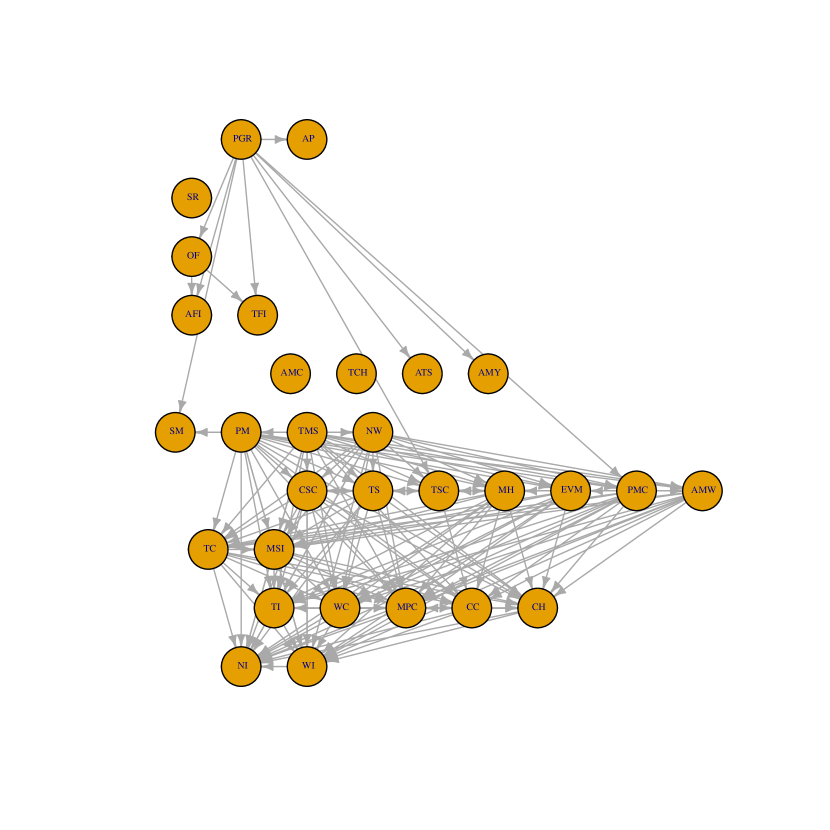
Figure 1: Estimated network for dairy cattle variables using partition with 10 groups

In order to understand/illustrate the difference in the performance of Partition-DAG with changes in the allocation of variables to partitions, we merged some of the $10$ groups to obtain a partition with $5$ groups, and again estimated a causal network using Partition-DAG. The estimated network with five groups is depicted in Figure 2.

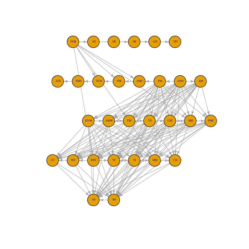
Figure 2: Estimated network for dairy cattle variables using partition with 5 groups

In addition to this partial ordering information, some relationships were known to exist; specifically, $38$ edges in total are known based on background information dictated by animal sciences theory, but also because some variables were explicitly computed using others. For the sake of clarity, we provide selected example next. It is well known that total dry matter intake ($TFI$) has a direct impact on milk yield ($AMY$) Hristov et al. (2004); in addition, the sign of this relationship is known to be positive. This last fact takes importance when evaluating the corresponding entries of the estimated Cholesky factor of the precision matrix (given their regression interpretation). Moreover, for economic variables it is easier to know what edges should exist in the estimated DAG because many economic indices are computed as linear combinations of other variables in the system. For instance, total production cost ($TC$) is the sum of partial costs such as reproductive management cost ($RMC$) and cost of soil correction strategies ($CSC$). Another example is net income ($NI$) which is the difference between total income ($TI$) and total cost ($TC$).

Since this extra information was not used by Partition-DAG, it allows us to carry out a partial evaluation of the performance of the proposed method. To this end, for the $5$ group case, $14$ out of the $31$ edges ($45\%$) were present in the estimated network, while in the $10$ group case, $17$ out of the $31$ edges ($55\%$) were present in the estimated network. The specific list of these edges and those present in the two estimated networks is given in Table 7.

Edge ($a\rightarrow b$)	Five Groups network	Ten Groups network
( NW , AMW )	Pres	Pres
( PM , AMW )	Abs	Pres
( TFI , AMY )	Abs	Abs
( TC , CC )	Abs	Pres
( TCH , CC )	Abs	Abs
( AP , CH )	Abs	Abs
( TC , CH )	Pres	Pres
( NW , CSC )	Pres	Pres
( TMS , CSC )	Pres	Abs
( AP , MH )	Abs	Abs
( PM , MH )	Abs	Pres
( SR , MH )	Abs	Abs
( PM , MPC )	Abs	Pres
( TC , MPC )	Abs	Pres
( EVM , MSI )	Pres	Pres
( TC , NI )	Pres	Pres
( TI , NI )	Pres	Pres
( SR , OF )	Pres	Abs
( AMY , PM )	Abs	Abs
( PMC , TC )	Abs	Pres
( SR , TCH )	Abs	Abs
( AFI , TFI )	Abs	Abs
( MSI , TI )	Pres	Pres
( ATS , TMS )	Abs	Abs
( AP , TS )	Abs	Abs
( TMS , TS )	Pres	Abs
( TMS , TSC )	Pres	Abs
( NW , WC )	Pres	Pres
( TC , WC )	Abs	Pres
( NW , WI )	Pres	Pres
( TI , WI )	Pres	Pres

Table 7: List of more known edges between dairy agroecosystem variables (in addition to the partition information), and whether these edges were present in the estimated networks

Also, a dairy science expert (Dr. Carulla, co-author) inspected all the estimated edges for each network, and identified which of the estimates edges were not meaningful. The following are some examples of incorrectly inferred edges because a direct causal relationship between the corresponding pair of variables does not exist: the economic value of milk ($EVM$) and production cost per liter ($MPC$), pasture growth rate (Growth rate) and total pasture area ($AP$), and growth rate and number of workers per month ($NW$). As to the first edge, total milk cost per litter is determined by total production cost and total milk yield, not by the economic value of milk. The price paid to the producer does not cause production cost. Regarding the second edge, it is not reasonable to state that total grazing area is caused by pasture growth rate. Total grazing area is explained by herd size and its productive targets (e.g., dairy and other agricultural activities), not by how fast its pastures grow. Finally, pasture growth rate cannot have a direct effect on the number of workers per month, because the later variable depends on social factors as well as on the productivity level, of course, growth rate affects ?productivity level and therefore, it could have an impact on the number of workers, but this does not imply a direct causal relationship. To summarize, for the $5$ group network, $19\%$ of the estimated edges were not meaningful, while for the $10$ group network, $17\%$ of the estimated edges were not meaningful. Once again, it can be seen that Partition-DAG is able to leverage additional external information (in the form of a finer partition) to improve performance.

The above analysis illustrates the tremendous usefulness of the application of the proposed method in dairy science and in the problem of DAG estimation more generally. In the first place, it is a sound approach to infer a DAG and the associated causal relationships from observational data in animal production systems using the available (partial) information, which is a feature exhibited by most of these agroecosystems. Further, knowledge of causal relationships in dairy and other animal production operations helps in taking management decisions and making recommendatios, since it leads to identifying what nodes have the biggest impact on the system outputs; the latter information singles out variables that should be modified and the direction of such modifications. Finally, the analysis of the estimated DAGs sheds light into interesting interactions between components of the production system and thus could be the basis to design follow-up experiments to fully test their validity.

References

- Altamore et al. [2013] D. Altamore, G. Consonni, and L. La Rocca. Objective Bayesian search of Gaussian directed acyclic graphical models for ordered variables with non-local priors. Biometrics, 69:478–487, 2013.
- Aragam and Zhou [2015] B. Aragam and Q. Zhou. Concave penalized estimation of sparse Gaussian Bayesian networks. Journal of Machine Learning Research, 16:2273–2328, 2015.
- Bargo et al. [2003] F. Bargo, L. D. Muller, E. S. Kolver, and J. E. Delahoy. Invited review: production and digestion of supplemented dairy cows on pasture. J Dairy Sci., 86:1–42, 2003.
- Cao et al. [2017] Xuan Cao, Kshitij Khare, and Malay Ghosh. Posterior graph selection and estimation consistency for high-dimensional Bayesian DAG models. https://arxiv.org/abs/1611.01205, 2017.
- Chickering [2003] David Maxwell Chickering. Optimal structure identification with greedy search. The Journal of Machine Learning Research, 3:507–554, 2003.
- Consonni et al. [2017] G. Consonni, L. La Rocca, and S. Peluso. Objective Bayes covariate-adjusted sparse graphical model selection. Scand. J. Statist, 44:741–764, 2017.
- Dillon [2006] P. Dillon. Achiving high dry-matter intake from pastures with grazing dairy cows. In A. Elgersma, J. Dijkstra, and S. Tamminga, editors, J. Dijkstra and S. Tamminga Fresh Herbage for Dairy Cattle, 1-26. Springer. Printed in the Netherlands. Springer, Netherlands, 2006.
- Elgersma et al. [2006] A. Elgersma, J. Dijkstra, and S. Tamminga. Fresh Herbage for Dairy Cattle. Springer, Netherlands, 2006.
- Ellis and Wong [2008] Byron Ellis and Wing Hung Wong. Learning causal Bayesian network structures from experimental data. Journal of the American Statistical Association, 103(482):778–789, 2008.
- Emmert-Streib et al. [2014] Frank Emmert-Streib, Matthias Dehmer, and Benjamin Haibe-Kains. Gene regulatory networks and their applications: understanding biological and medical problems in terms of networks. Frontiers in Cell and Developmental Biology, 2:38, 2014.
- Gamez et al. [2011] Jose A Gamez, Juan L Mateo, and Jose M Puerta. Learning bayesian Networks by hill climbing: Efficient methods based on progressive restriction of the neighborhood. Data Mining and Knowledge Discovery, 22(1-2):106–148, 2011.
- Gamez et al. [2012] Jose A Gamez, Juan L Mateo, and Jose M Puerta. One iteration chc algorithm for learning bayesian networks: An effective and efficient algorithm for high dimensional problems. Progress in Artificial Intelligence, 1(4):329–346, 2012.
- Geiger and Heckerman [2013] Dan Geiger and David Heckerman. Learning Gaussian networks. arXiv:1302.6808, 2013.
- Heckerman et al. [1995] David Heckerman, Dan Geiger, and David M Chickering. Learning Bayesian networks: The combination of knowledge and statistical data. Machine learning, 20(3):197–243, 1995.
- Hristov et al. [2004] A. N. Hristov, W. J. Price, and B. Shafii. A meta-analysis examining the relationship among dietary factors, dry matter intake, and milk and milk protein yield in dairy cows. J Dairy Sci., 87:2184–2196, 2004.
- Huang et al. [2006] J. Huang, N. Liu, M. Pourahmadi, and L. Liu. Covariance selection and estimation via penalised normal likelihoode. Biometrika, 93:85–98, 2006.
- Jalvingh [1992] A.W. Jalvingh. The possible role of existing models in on-farm decision support in dairy cattle and swine production. Livestock Production Science, 31:355–365, 1992.
- Kalisch and Buhlmann [2007] M. Kalisch and P. Buhlmann. Estimating high-dimensional directed acyclic graphs with the pc-algorithm. Journal of Machine Learning Research, 8:613–636, 2007.
- Kalisch and B¨uhlmann [2007] Markus Kalisch and Peter B¨uhlmann. Estimating high-dimensional directed acyclic graphs with the pc-algorithm. The Journal of Machine Learning Research, 8:613–636, 2007.
- Khare et al. [2017] Kshitij Khare, Sang Oh, Syed Rahman, and Bala Rajaratnam. A convex framework for high-dimensional sparse Cholesky based covariance estimation. https://arxiv.org/abs/1610.02436, 2017.
- Lam and Bacchus [1994] Wai Lam and Fahiem Bacchus. Learning Bayesian belief networks: An approach based on the MDL principle. Computational Intelligence, 10(3):269–293, 1994.
- Marbach et al. [2009] Daniel Marbach, Thomas Schaffter, Claudio Mattiussi, and Dario Floreano. Generating Realistic In Silico Gene Networks for Performance Assessment of Reverse Engineering Methods. Journal of Computational Biology, 16(2):229–239, 2009. 10.1089/cmb.2008.09TT. WingX.
- Marbach et al. [2010] Daniel Marbach, Robert J. Prill, Thomas Schaffter, Claudio Mattiussi, Dario Floreano, and Gustavo Stolovitzky. Revealing strengths and weaknesses of methods for gene network inference. PNAS, 107(14):6286–6291, 2010. 10.1073/pnas.0913357107. WingX.
- Marbach et al. [2012] Daniel Marbach, James C Costello, Robert Küffner, Nicole M Vega, Robert J Prill, Diogo M Camacho, Kyle R Allison, Andrej Aderhold, Richard Bonneau, Yukun Chen, et al. Wisdom of crowds for robust gene network inference. Nature methods, 9(8):796, 2012.
- Prill et al. [2010] Robert J. Prill, Daniel Marbach, Julio Saez-Rodriguez, Peter K. Sorger, Leonidas G. Alexopoulos, Xiaowei Xue, Neil D. Clarke, Gregoire Altan-Bonnet, and Gustavo Stolovitzky. Towards a rigorous assessment of systems biology models: The DREAM3 challenges. PLOS ONE, 5(2):1–18, 02 2010. 10.1371/journal.pone.0009202. URL https://doi.org/10.1371/journal.pone.0009202.
- Shojaie and Michailidis [2010] A. Shojaie and G. Michailidis. Penalized likelihood methods for estimation of sparse high-dimensional directed acyclic graphs. Biometrika, 97:519–538, 2010.
- Shojaie et al. [2014] A. Shojaie, A. Jauhiainen, M. Kallitsis, and G. Michailidis. Inferring regulatory networks by combining perturbation screens and steady state gene expression profiles. PLoS ONE, 9:e82393, 2014.
- Spirtes et al. [2001] Peter Spirtes, Clark Glymour, and Richard Scheines. Causation, Prediction, and Search. 2001.
- Thornley and France [2007] J.H.M. Thornley and J. France. Mathematical models in agriculture. Quantitative methods for Plant, Animal and Ecological sciences. Cromwell Press Trowbridge, UK, 2nd edition edition, 2007.
- Tsamardinos et al. [2006] Ioannis Tsamardinos, Laura E Brown, and Constantin F Aliferis. The max-min hill-climbing Bayesian network structure learning algorithm. Machine Learning, 65(1):31–78, 2006., 65(1):31–78, 2006.
- Tseng [2001] P. Tseng. Convergence of a block coordinate descent method for nondifferentiable minimization. Journal of Optimization Theory and Applications, 109:475–494, 2001.
- Tsoumakas et al. [2010] G. Tsoumakas, I. Katakis, and I. P. Vlahavas. Mining multi-label data. In O. Maimon and L. Rokach, editors, Data Mining and Knowledge Discovery Handbook, pages 667–685. Springer-Verlag, Heidelberg, Germany, 2010.
- van de Geer and Buhlmann [2013] S. van de Geer and P. Buhlmann. l0-penalized maximum likelihood for sparse directed acyclic graphs. Annals of Statistics, 41:536–567, 2013.
- Zhou [2011] Qing Zhou. Multi-domain sampling with applications to structural inference of Bayesian networks. Journal of the American Statistical Association, 106(496):1317–1330, 2011.