Helical Miura Origami

Abstract

We characterize the phase-space of all Helical Miura Origami. These structures are obtained by taking a partially folded Miura parallelogram as the unit cell, applying a generic helical or rod group to the cell, and characterizing all the parameters that lead to a globally compatible origami structure. When such compatibility is achieved, the result is cylindrical-type origami that can be manufactured from a suitably designed flat tessellation and “rolled-up” by a rigidly foldable motion into a cylinder. We find that the closed Helical Miura Origami are generically rigid to deformations that preserve cylindrical symmetry, but multistable. We are inspired by the ways atomic structures deform feng2019phase to develop two broad strategies for reconfigurability: motion by slip, which involves relaxing the closure condition; and motion by phase transformation, which exploits multistability. Taken together, these results provide a comprehensive description of the phase-space of cylindrical origami, as well as quantitative design guidance for their use as actuators or metamaterials that exploit twist, axial extension, radial expansion, and symmetry.

Origami is the ancient Japanese art of paper folding. In recent years, this art form has been appreciated not only for its aesthetics , but also for its potential functionality peraza2014origami —including in space technologies wilson2013origami ; schenk2013inflatable , transforming architectures reis2015transforming ; tachi2011designing , multistability and topological properties waitukaitis2015origami ; waitukaitis2016origami ; chen2016topological , biological structures Faber1386 ; DNAorigami ; han2011dna , deployable antennas Liu_helical_antenna_2014 ; yao2014novel , metamaterials schenk2013geometry ; yasuda2015reentrant ; silverberg2014using , and mechanical properties wei2013geometric ; ftp_PNAS_2015 ; dudte2016programming . Origami design utilizes the shape change induced by piecewise affine isometric deformations (i.e., folding along creases)—from, say, an easy-to-manufacture flat reference sheet with a pre-designed folding crease pattern—to achieve a desired configuration in 3-D space. We call such designs rigidly foldable if each panel can rotate along the folding crease lines and remain rigid (without stretch or flexure) during the folding process. The classical Miura origami pattern miura_93 is the simplest example of this type, and its generalizations lead to the study of systems of equations that are highly nonlinear and geometrically constrained. As a result, characterizing global properties of broad classes of origami structures—such as whether they are rigid, multistable or rigidly foldable—is a challenge that has attracted significant research interest. One way to study this problem is by using iterative algorithms that enforce a certain topology and foldability paul_miura ; bowers2015lang ; dudte2016programming ; lh_RFF_2018 . Another approach is to focus on patterns consistent with a certain symmetry.

In this work, we follow the symmetry approach to characterize, in a quite general way, Helical Miura Origami (HMO). These are cylindrical type origami obtained by repeated application of a helical or rod group to a partially folded unit cell, which we call a Miura parallelogram. In this procedure, the parameters are kept completely general and on full display, and we are able to address the global problem of closing the cylinder by a straightforward numerical algorithm. In group theory language “closing the cylinder” is ensuring the group is discrete. As a result, we can completely characterize the phase-space of all HMO, i.e., all cylindrical origami consistent with helical or rod symmetry and the Miura parallelogram as the unit cell. By exhaustive numerical treatment, we find that HMO are generically rigid to deformations that preserve cylindrical symmetry, but multistable. This rigidity is not all that surprising; the well-known cylindrical origami are either rigid (for example the Yoshimura pattern wang2011folding ; bos_incompressibility_2016 , Kresling pattern jianguo2015bistable ) or they lose the cylindrical symmetry while folding tachi2009generalization . Nevertheless, we show that reconfigurability can be achieved. Inspired by atomistic theory, we discuss two strategies for doing so: one involving motion by slip and the other involving phase transformation.

Characterization of a Miura parallelogram. We begin by analyzing the kinematics of a parallelogram with a four-fold vertex satisfying the Kawasaki’s condition: “opposite sector angles sum to $\pi$”. This defines a Miura parallelogram unit cell (Fig. 1(a)) with $\angle{\bf x}_{1}{\bf x}_{0}{\bf x}_{2}+\angle{\bf x}_{4}{\bf x}_{0}{\bf x}_{3}=\pi$, where $0<\angle{\bf x}_{i}{\bf x}_{j}{\bf x}_{k}<\pi$ is the angle between ${\bf x}_{k}-{\bf x}_{j}$ and ${\bf x}_{i}-{\bf x}_{j}$ . To characterize an isometric (piecewise rigid) folding of this crease pattern, we fix one of the panels by setting $\mathbf{y}({\bf x}_{i})=\mathbf{x}_{i},\ i=0,1,2$, without loss of generality. In our notation ${\bf y}({\bf x})$ represents the deformation from the flat state in Lagrangian form (see the Supplement). The kinematics of this pattern (i.e., its deformation gradients) are then described by a composition of $3\times 3$ rotation matrices $\mathbf{R}_{i}(\gamma_{i})$ whose axes are tangent to the crease pattern $\mathbf{x}_{i}-\mathbf{x}_{0}$ in flat state . Specifically, the necessary and sufficient condition for isometric origami is

$$\mathbf{R}_{1}(\gamma_{1}){\bf R}(\gamma_{2}){\bf R}_{3}(\gamma_{3}){\bf R}_{4}(\gamma_{4})=\mathbf{I}.$$ (1)

Note, the solutions of this equation describe a folding where panels deform as depicted in Fig. 1(a-b). Further, a positive folding angle describes a valley and a negative a mountain here (red and blue, respectively, in Fig. 1(b)).

By solving (1), we derive the full kinematics of the Miura parallelogram. Generically, the solutions are described by a continuous one-parameter family for which the four folding angles $(\gamma_{1},\gamma_{2},\gamma_{3},\gamma_{4})$ are given by the following expression:

$$\gamma_{1}=-\sigma\bar{\gamma}_{3}^{\sigma}(\omega),~{}\gamma_{2}=\sigma\omega,~{}\gamma_{3}=\bar{\gamma}_{3}^{\sigma}(\omega),~{}\gamma_{4}=\omega,$$ (2)

$$\bar{\gamma}_{3}^{\sigma}(\omega)=\text{sign}\Big{(}(c_{\alpha}-\sigma c_{\beta})\omega\Big{)}\arccos\Big{(}\tfrac{(\sigma 1-c_{\alpha}c_{\beta})c_{\omega}+s_{\alpha}s_{\beta}}{(\sigma 1-c_{\alpha}c_{\beta})+s_{\alpha}s_{\beta}c_{\omega}}\Big{)},$$

$$\sigma\in\mathcal{A}=\begin{cases}\emptyset&\text{ if }\alpha=\beta=\tfrac{\pi}{2}\\ \{-\}&\text{ if }\alpha=\beta\neq\tfrac{\pi}{2}\\ \{+\}&\text{ if }\alpha=\pi-\beta\neq\tfrac{\pi}{2}\\ \{\pm\}&\text{ otherwise.}\end{cases}$$

Here, $\sigma\in\mathcal{A}$ denotes one of the (at most) two branches of solutions corresponding to different mountain-valley crease assignments, the folding angles are parameterized by $-\pi\leq\omega\leq\pi$, and we employ the shorthand notation $c_{\theta}=\cos(\theta)$, $s_{\theta}=\sin(\theta)$, $\alpha=\angle{\bf x}_{1}{\bf x}_{0}{\bf x}_{2}$ and $\beta=\angle{\bf x}_{2}{\bf x}_{0}{\bf x}_{3}$. In addition to this generic family, there is a degenerate family of solutions for certain Miura parallelograms; specifically, those characterized by a solution branch $\sigma=+$ or $-$ that does not belong to $\mathcal{A}$. These cases describe folding-in-half along a single crease:

$$\begin{cases}\gamma_{1,3}=0,~{}\gamma_{2,4}=\omega&\text{ if }\sigma=+,\alpha=\beta\\ \gamma_{1,3}=\omega,~{}\gamma_{2,4}=0&\text{ if }\sigma=-,\alpha=\pi-\beta\end{cases}$$ (3)

for the folding parameter $-\pi\leq\omega\leq\pi$. We provide a brief derivation of these results in the Supplement, and this viewpoint of the kinematics of origami is further developed in paul_miura .

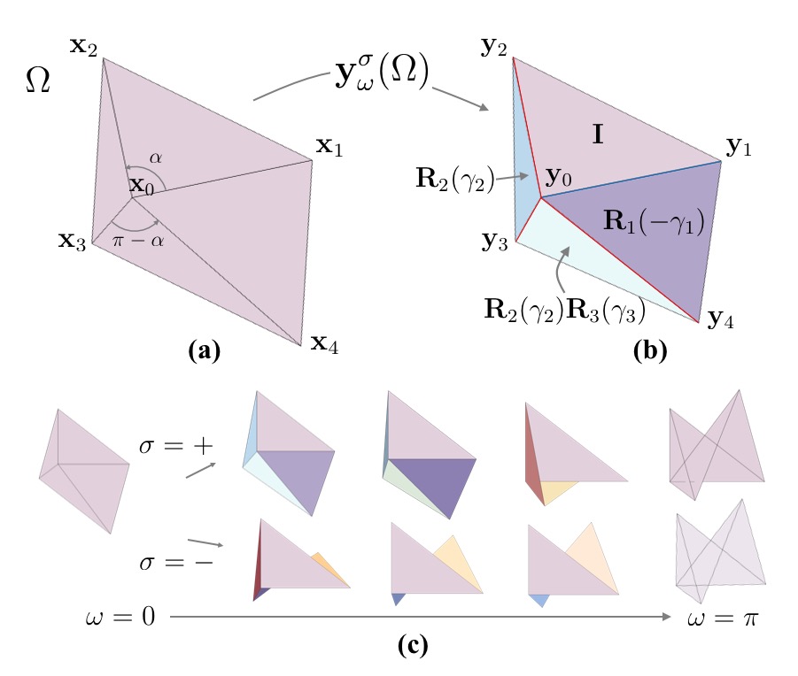
Figure 1: The folding kinematics of Miura parallelograms. (a) The crease pattern prior to folding. (b) The kinematics are described by a deformation $\mathbf{y}^{\sigma}_{\omega}(\Omega)$ whose gradients are as depicted, i.e., rotations of the panels along the creases that are subject to the compatibility condition (1). (c) There are exactly two continuous one parameter families which take the Miura parallelogram from flat ($\omega=0$) to folded flat $(\omega=\pm\pi)$ as rigidly foldable origami. The two branches correspond to distinct mountain-valley assignments, as indicated with $\sigma=\pm$.

The folding angle parameterizations (LABEL:kin1) and (3) are sufficient and (with a minor caveat ) necessary for solving (1) and, as such, completely characterize the folding of a Miura parallelogram. Importantly, the parameterizations highlight two universal features of kinematics: There are two branches of solutions $\sigma=\pm$ corresponding to the different mountain-valley crease assignments, and each branch is described by a single folding parameter $\omega$. Accordingly, the explicit folding deformation is a continuous piecewise rigid deformation $\mathbf{y}_{\omega}^{\sigma}\colon\Omega\rightarrow\mathbb{R}^{3}$ with deformation gradients as shown in Fig. 1(a) for $\gamma_{1,2,3,4}\equiv\gamma_{1,2,3,4}(\omega,\sigma)$ satisfying one of the parameterizations in (LABEL:kin1-3). This furnishes the deformed unit cell ${\bf y}^{\sigma}_{\omega}(\Omega)$ with corner positions ${\bf y}_{i}={\bf y}^{\sigma}_{\omega}({\bf x}_{i}),i=1,2,3,4$ after folding . These observations are known in a different way in the literature on origami, but it will be important for our purposes to write the deformation explicitly.

To construct the HMO, we will apply rotations and translations to ${\bf y}^{\sigma}_{\omega}(\Omega)$ that map one side of the deformed unit cell to its opposite side. Thus, as a final point of characterization for the unit cell, we require the parallelogram condition to hold (i.e., $|{\bf x}_{4}-{\bf x}_{3}|=|{\bf x}_{1}-{\bf x}_{2}|$ and $|{\bf x}_{1}-{\bf x}_{4}|=|{\bf x}_{2}-{\bf x}_{3}|$). This condition, combined with Kawasaki’s condition, constrains the four creases $\mathbf{x}_{i}-\mathbf{x}_{0}$. We parameterize these two conditions up to a trivial rescaling, rotation and translation as follows: We assume $|\mathbf{x}_{2}-\mathbf{x}_{1}|=|\mathbf{x}_{4}-\mathbf{x}_{3}|=1$ without loss of generality , and we introduce the angle between $\mathbf{x}_{2}-\mathbf{x}_{1}$ and $\mathbf{x}_{4}-\mathbf{x}_{1}$ as $\eta$ (where $0<\eta<\pi$), and the length $|\mathbf{x}_{4}-\mathbf{x}_{1}|=|\mathbf{x}_{3}-\mathbf{x}_{2}|=l>0$. This completely parameterizes the boundary of the parallelogram (Fig. 2(a)). Additionally, we show in the Supplement that the creases satisfy Kawasaki’s condition if and only if the vertex $\mathbf{x}_{0}$ lies on one of two curves in the interior of the parallelogram pictured in red in Fig. 2 These curves are parameterized as follows.

1. Case $l>1$: The two curves are given by ${\bf x}_{0}(\lambda)={\bf x}_{1}+\lambda({\bf x}_{2}-{\bf x}_{1})+f^{\pm}(\lambda)({\bf x}_{4}-{\bf x}_{1})$, where $0<\lambda<1$ and the two functions $f^{\pm}$ satisfy

   $$f^{\pm}(\lambda)=\frac{1}{2}\pm\sqrt{\frac{1}{l^{2}}\big{(}\lambda-\frac{1}{2}\big{)}^{2}+\frac{1}{l^{2}}\frac{l^{2}-1}{4}}.$$ (4)

2. Case $l<1$: The two curves are given by ${\bf x}_{0}(\lambda)={\bf x}_{1}+\lambda({\bf x}_{4}-{\bf x}_{1})+g^{\pm}(\lambda)({\bf x}_{2}-{\bf x}_{1})$, where $0<\lambda<1$ and the two functions $g^{\pm}$ satisfy

   $$g^{\pm}(\lambda)=\frac{1}{2}\pm\sqrt{l^{2}\big{(}\lambda-\frac{1}{2}\big{)}^{2}+\frac{1-l^{2}}{4}}.$$ (5)

3. Case $l=1$: The two curves are given by $\mathbf{x}_{0}(\lambda)=\lambda\mathbf{x}_{2}+(1-\lambda)\mathbf{x}_{4}$ and $\mathbf{x}_{0}(\lambda)=\lambda\mathbf{x}_{1}+(1-\lambda)\mathbf{x}_{3}$ for $0<\lambda<1$.

As there is an underlying reflection symmetry to this geometry of these curves, we are free to restrict our attention to either the $+$ or $-$ case in (i-iii) without loss of generality. This fully defines the crease pattern.

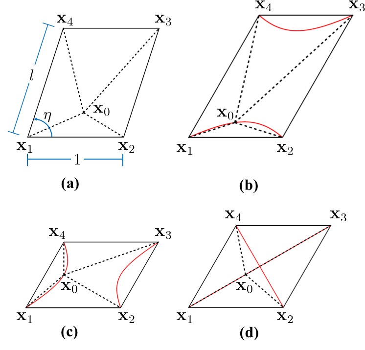
Figure 2: The reference geometry of a Miura parallelogram. (a) The boundary of the parallelogram is parameterized by $\eta$ and $l$ (up to a uniform rescaling). (b-d) The admissible curves on which the interior vertex satisfies Kawasaki’s condition are shown in red. There are three cases, each parameterized by a $\lambda$ taking values in the interval $(0,1)$.

To summarize, the parameters $(\eta,l,\lambda,\omega,\sigma)$ given above completely characterize all possible Miura parallelograms—up to trivial rescaling, translation, overall rigid rotation, and reflection—and all possible ways of folding origami using these parallelograms.

HMO are objective structures. We now define precisely what it means for a structure to be HMO, and we discuss the implications of this definition as it relates to characterizing all such structures. The line of thinking here is based on a systematic and complete characterization of helical and rod symmetry that we developed for an analogous problem: describing all possible phases in nanotubes feng2019phase . To avoid being redundant, we simply borrow (and state without proof) many ideas from this work that are used in the constructions here.

Briefly, we define an HMO as any compatible origami structure obtained by a suitable group action $\mathcal{G}$ (see below) on the partially folded Miura parallelogram $\mathbf{y}_{\omega}^{\sigma}(\Omega)$. The groups we consider are discrete, Abelian (i.e., the elements commute), contain only isometries, and have an orbit $\{g(\mathbf{x})\colon g\in\mathcal{G}\}$ for each point $\mathbf{x}\in\mathbb{R}^{3}$ that gives a collection of points that all lie on a cylinder. (The cylinders can be different for different choices of ${\bf x}$.) This means that every Miura parallelogram in the structure “sees the same environment” james_JMPS_06 , which is the natural generalization of periodicity to cylindrical origami.

An isometry is simply a map $g=(\mathbf{R}|\mathbf{c})$ defined by $g(\mathbf{x})=\mathbf{R}\mathbf{x}+\mathbf{c}$, where $\mathbf{R}$ is a $3\times 3$ orthogonal matrix and $\mathbf{c}\in\mathbb{R}^{3}$. Below, we use O(3) to denote the $3\times 3$ orthogonal matrices, and SO(3) to denote rotations (i.e., the subset of O(3) with determinant $+1$). One can multiply isometries $g_{1}=(\mathbf{R}_{1}|\mathbf{c}_{1})$ and $g_{2}=(\mathbf{R}_{2}|\mathbf{c}_{2})$ using the standard rule $g_{1}g_{2}=({\bf R}_{1}{\bf R}_{2}|{\bf c}_{1}+{\bf R}_{1}{\bf c}_{2})$. Under this rule, the collection of all isometries is a group, and it has many subgroups. Thus, one might worry that the aforementioned—and rather general—family of groups lacks meaningful structure. Strikingly though (and this is made precise in feng2019phase ), discrete and Abelian isometry groups subject to the stated cylinder condition are quite restrictive. They must be described as the product of powers of two generators on the set of pairs of integers $\mathbb{Z}^{2}$, i.e.,

$$\mathcal{G}=\{g_{1}^{p}g_{2}^{q}\colon(p,q)\in\mathbb{Z}^{2}\},$$ (6)

in which the generators of the group $g_{1}$ and $g_{2}$ are two screw isometries

$$g_{i}=({\bf R}_{\theta_{i}}|\tau_{i}{\bf e}+({\bf I}-{\bf R}_{\theta_{i}}){\bf z}),\;\;~{}i=1,2,$$ (7)

with parameters $\mathbf{R}_{\theta_{i}}\in$ SO(3), $-\pi<\theta_{i}\leq\pi$, $\tau_{i}\in\mathbb{R}$, $\mathbf{e}\in\mathbb{R}^{3}$, $|\mathbf{e}|=1$, and $\mathbf{z}\in\mathbb{R}^{3}$, $\mathbf{z}\cdot\mathbf{e}=0$ characterizing the rotation, rotation angle, translation, rotation axis and origin of the isometry, respectively. These parameters are subject to a discreteness condition

$$\begin{cases}p^{\star}\tau_{1}+q^{\star}\tau_{2}=0\\ p^{\star}\theta_{1}+q^{\star}\theta_{2}=2\pi\end{cases}$$ (8)

for some pair of integers $(p^{\star},q^{\star})\in\mathbb{Z}^{2}$. Technically, we should also enforce $\tau_{1}^{2}+\tau_{2}^{2}>0$, as the violation of this condition results in a flattened ring rather than a cylinder. However, we avoid this restriction since the flattened ring is of technological interest: the folded flat portion of the Kresling pattern in Fig. 7(d) is one example.

Finally, we should point out the groups $\mathcal{G}$ in (6) are not uniquely described by a single parameterization satisfying (7-8). This should not be unexpected. In periodic structures, there are many equivalent choices of lattice vectors which generate the same lattice. In fact, the degeneracy here—much like the 2-D lattice—is fully characterized by a $\boldsymbol{\mu}\in GL(\mathbb{Z}^{2})$. Here, $GL(\mathbb{Z}^{2})$ is the set of $2\times 2$ matrices with integer entries and determinant $\pm 1$. That is, for any group $\mathcal{G}$ satisfying (6-8), we can replace the parameters by a linear transformation $(\theta_{1},\theta_{2})\mapsto\boldsymbol{\mu}(\theta_{1},\theta_{2})$, $(\tau_{1},\tau_{2})\mapsto\boldsymbol{\mu}(\tau_{1},\tau_{2})$, and $(p^{\star},q^{\star})\mapsto\boldsymbol{\mu}^{-T}(p^{\star},q^{\star})$ and generate the same structure (i.e., $\mathcal{G}=\mathcal{G}_{\boldsymbol{\mu}}$) if $\boldsymbol{\mu}\in GL(\mathbb{Z}^{2})$.

Thus, the aim in what follows is to characterize the sets of parameters $(\eta,l,\lambda,\omega,\sigma,\theta_{1,2},\tau_{1,2},\mathbf{e},\mathbf{z},p^{\star},q^{\star})$ (up to this trivial degeneracy $\boldsymbol{\mu}\in GL(\mathbb{Z}^{2}))$ that lead to a fully compatible cylindrical origami structure. This then captures the phase-space of all HMO.

Design equations for HMO. These are obtained systematically by satisfying all compatibility conditions, i.e., the conditions under which the folded tiles of the structure fit together perfectly without gaps. For developing these ideas, we find it convenient to introduce the tessellation $\mathcal{T}\Omega=\{g(\Omega)\colon g\in\mathcal{T}\}$ for the translation group $\mathcal{T}=\{t_{1}^{p}t_{2}^{q}\colon(p,q)\in\mathbb{Z}^{2}\}$ such that $t_{1}=(\mathbf{I}|\mathbf{x}_{1}-\mathbf{x}_{4})$ and $t_{2}=(\mathbf{I}|\mathbf{x}_{2}-\mathbf{x}_{1})$. Since

$$t_{1}(\mathbf{x}_{4})=\mathbf{x}_{1},\quad t_{2}(\mathbf{x}_{3})=\mathbf{x}_{2},$$ (9)

$$t_{2}(\mathbf{x}_{1})=\mathbf{x}_{2},\quad t_{2}(\mathbf{x}_{4})=\mathbf{x}_{3},$$

this gives a tessellated plane in $\mathbb{R}^{3}$ of Miura parallelograms prior to folding. Suitably defined strips of this tessellation will be used to construct the HMO from this easy-to-manufacture flat state (e.g., Fig 3).

We begin with local compatibility: Consider a partially folded Miura parallelogram $\mathbf{y}_{\omega}^{\sigma}(\Omega)$ with it corners denoted as $\mathbf{y}_{i}$, $i=1,2,3,4$ (Fig. 1(a)), consider a group $\mathcal{G}$ satisfying (6-8), and consider the structure $\mathcal{G}\mathbf{y}_{\omega}^{\sigma}(\Omega)=\{g_{1}^{p}g_{2}^{q}(\mathbf{y}_{\omega}^{\sigma}(\Omega))\colon(p,q)\in\mathbb{Z}^{2}\}$. The nearest neighbors to $\mathbf{y}_{\omega}^{\sigma}(\Omega)$ on the structure are, therefore, obtained by the application of group elements to this domain. Without loss of generality , we assume the neighbor to the“left” of the unit cell is $g_{1}(\mathbf{y}_{\omega}^{\sigma}(\Omega))$ and the neighbor “above” the unit cell is $g_{2}(\mathbf{y}_{\omega}^{\sigma}(\Omega))$. Then, one condition of compatibility is that the unit cell is connected to its neighbors; particularly, to its neighbor on the left along the line $\ell_{23}=\{\delta\mathbf{y}_{2}+(1-\delta)\mathbf{y}_{3}\colon 0\leq\delta\leq 1\}$ and to its neighbor up above along the line $\ell_{12}=\{\delta\mathbf{y}_{1}+(1-\delta)\mathbf{y}_{2}\colon 0\leq\delta\leq 1\}$. This gives four restrictions on the group elements:

$$g_{1}(\mathbf{y}_{4})=\mathbf{y}_{1},\quad g_{1}(\mathbf{y}_{3})=\mathbf{y}_{2},$$ (10)

$$g_{2}(\mathbf{y}_{1})=\mathbf{y}_{2},\quad g_{2}(\mathbf{y}_{4})=\mathbf{y}_{3},$$

which we term local compatibility.

The reason for the terminology is that (10) is a discrete and symmetry-related version of the local curl-free and jump compatibility conditions that indicate whether a prescribed deformation gradient can describe a continuous deformation on a simply connected domain. Indeed, $g_{1}$ and $g_{2}$ are commutative (i.e., $g_{1}g_{2}=g_{2}g_{1}$) under the multiplication rule $g_{1}g_{2}({\bf x})=g_{1}(g_{2}({\bf x}))$. This means that $g_{1}$ and $g_{2}$ satisfy the loop condition $g_{1}g_{2}({\bf y}_{i})=g_{2}g_{1}({\bf y}_{i})$. As a result, the four nearest neighbor Miura parallelograms ${\bf y}_{\omega}^{\sigma}(\Omega)$, $g_{1}({\bf y}_{\omega}^{\sigma}(\Omega))$, $g_{2}({\bf y}_{\omega}^{\sigma}(\Omega))$ and $g_{1}g_{2}({\bf y}_{\omega}^{\sigma}(\Omega))=g_{2}g_{1}({\bf y}_{\omega}^{\sigma}(\Omega))$ fit together automatically whenever (10) holds. Combining (9) and (10), it then follows that the induced deformation given by

$$\mathbf{y}(t_{1}^{p}t_{2}^{q}(\mathbf{x}))=g_{1}^{p}g_{2}^{q}(\mathbf{y}_{\omega}^{\sigma}(\mathbf{x})),~{}\forall~{}\mathbf{x}\in\overline{\Omega},~{}(p,q)\in\mathbb{Z}^{2}$$ (11)

is a continuous isometric origami deformation that maps the tessellated plane to the origami structure. This is the key advantage of bringing out the group structure: simply solve the four equations (10), and the entire structure fits together perfectly without gaps (11).

In the Supplement, we solve the conditions of local compatibility (10) explicitly. To explain the parameterization obtained, we assume the Miura parallelogram is partially folded (i.e., $-\pi<\omega<\pi$ and $\omega\neq 0$), and we let the side length vectors be given by $\mathbf{u}_{a}=\mathbf{y}_{3}-\mathbf{y}_{4}$, $\mathbf{u}_{b}=\mathbf{y}_{2}-\mathbf{y}_{1}$, $\mathbf{v}_{a}=\mathbf{y}_{1}-\mathbf{y}_{4}$ and $\mathbf{v}_{b}=\mathbf{y}_{2}-\mathbf{y}_{3}$. We can then always define the right-hand orthonormal frame $\{\mathbf{f}_{1},\mathbf{f}_{2},\mathbf{f}_{3}\}$,

$$\mathbf{f}_{1}=\frac{\mathbf{u}_{a}+\mathbf{u}_{b}}{|\mathbf{u}_{a}+\mathbf{u}_{b}|},~{}\mathbf{f}_{2}=\frac{\mathbf{u}_{a}\times\mathbf{u}_{b}}{|\mathbf{u}_{a}\times\mathbf{u}_{b}|},~{}\mathbf{f}_{3}=\frac{\mathbf{u}_{a}-\mathbf{u}_{b}}{|\mathbf{u}_{a}-\mathbf{u}_{b}|}$$ (12)

(since $\omega\neq 0,\pm\pi$ implies $\mathbf{u}_{a}\times\mathbf{u}_{b}\neq 0$). The necessary and sufficient conditions for local compatibility in this setting are thus

$$\mathbf{e}\equiv\mathbf{e}^{\sigma}(\omega,\varphi)=c_{\varphi}\mathbf{f}_{1}+s_{\varphi}\mathbf{f}_{2},$$ (13)

$$\theta_{1}\equiv\theta_{1}^{\sigma}(\omega,\varphi)=\text{sign}(\mathbf{e}\cdot(\mathbf{u}_{a}\times\mathbf{u}_{b}))\arccos\Big{(}\frac{\mathbf{u}_{a}\cdot\mathbf{P}_{\mathbf{e}}\mathbf{u}_{b}}{|\mathbf{P}_{\mathbf{e}}\mathbf{u}_{a}|^{2}}\Big{)},$$

$$\theta_{2}\equiv\theta_{2}^{\sigma}(\omega,\varphi)=\text{sign}(\mathbf{e}\cdot(\mathbf{v}_{a}\times\mathbf{v}_{b}))\arccos\Big{(}\frac{\mathbf{v}_{a}\cdot\mathbf{P}_{\mathbf{e}}\mathbf{v}_{b}}{|\mathbf{P}_{\mathbf{e}}\mathbf{v}_{a}|^{2}}\Big{)},$$

$$\tau_{1}\equiv\tau_{1}^{\sigma}(\omega,\varphi)=\mathbf{e}\cdot\mathbf{v}_{a},\quad\tau_{2}\equiv\tau_{2}^{\sigma}(\omega,\varphi)=\mathbf{e}\cdot\mathbf{u}_{a},$$

$$\mathbf{z}\equiv\mathbf{z}^{\sigma}(\omega,\varphi)=(\mathbf{I}-\mathbf{R}_{\theta_{1}}+\mathbf{e}\otimes\mathbf{e})^{-1}\mathbf{P}_{\mathbf{e}}(\mathbf{y}_{2}-\mathbf{R}_{\theta_{1}}\mathbf{y}_{3}),$$

where $\mathbf{P}_{\mathbf{e}}=\mathbf{I}-\mathbf{e}\otimes\mathbf{e}$ denotes the linear transformation that projects vectors onto the plane with normal $\mathbf{e}$ and the angle $-\pi/2<\varphi\leq\pi/2$ (describing the axis $\mathbf{e}$) is a free parameter . For completeness, note that the fully folded cases $\omega=\pm\pi$ and fully unfolded case $\omega=0$ are of course included (see the Supplement). For definiteness, we will focus on the solutions governed by (LABEL:paramLocal). Examples of the exceptional cases are fully degenerate cylinders ($\omega=0$) or flattened ring structures $(\omega=\pi)$.

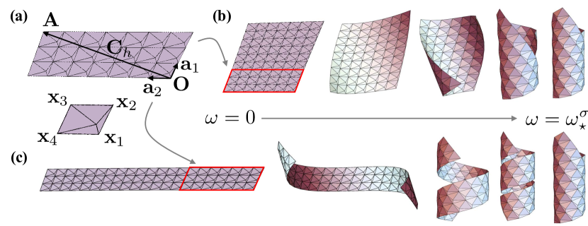
Figure 3: Constructing an HMO from a flat tessellation. (a) Each HMO is characterized by a chiral vector $\mathbf{C}_{h}=\overrightarrow{\bf OA}=p^{\star}{\bf a}_{1}+q^{\star}{\bf a}_{2}$, which is a linear combination of the side length vectors $\mathbf{a}_{1}=\mathbf{x}_{2}-\mathbf{x}_{1}$ and $\mathbf{a}_{2}=\mathbf{x}_{4}-\mathbf{x}_{1}$. This describes a $(p^{\star},q^{\star})$ building block for the structure. (b-c) In extending this building block to a tessellated strip in the “vertical” (b) or “horizontal” (c) direction, an HMO structure is achieved by a rigidly foldable motion that connects the points $\mathbf{O}$ and $\mathbf{A}$ at $\omega=\omega_{\star}^{\sigma}$ (i.e., the angle(s) solving (15)).

Importantly, the corners $\mathbf{y}_{i}$, $i=1,2,3,4$ (and thereby $\mathbf{u}_{a,b},\mathbf{v}_{a,b},$ and $\mathbf{f}_{1,2,3}$ above) depend only on the folding parameter $\omega$ and the mountain-valley assignment $\sigma$. Consequently, after satisfying local compatibility, the kinematic freedom in (LABEL:paramLocal) is $-\pi<\omega<\pi,\ \omega\neq 0,\ -\pi/2<\varphi\leq\pi/2$ and $\sigma=\pm$. We utilize this freedom to solve the discreteness condition (8). This, in turn, is equivalent to closing the cylinder; see Fig. 3.

Indeed, given integers $(p^{\star},q^{\star})$, not both zero, we observe that the discreteness condition (i.e., $p^{\star}\tau_{1}+q^{\star}\tau_{2}=0$) uniquely determines the angle $\varphi$ under the parameterization (LABEL:paramLocal). The explicit form is

$$\varphi\equiv\varphi_{\star}^{\sigma}(\omega)=\arctan\Big{(}\frac{-\mathbf{f}_{1}\cdot(p^{\star}\mathbf{v}_{a}+q^{\star}\mathbf{u}_{a})}{\mathbf{f}_{2}\cdot(p^{\star}\mathbf{v}_{a}+q^{\star}\mathbf{u}_{a})}\Big{)}.$$ (14)

(Note, $\varphi\equiv\varphi_{\star}^{\sigma}(\omega)=\pi/2$ if $\mathbf{f}_{2}\cdot(p^{\star}\mathbf{v}_{a}+q^{\star}\mathbf{u}_{a})=0$, and $p^{\star}\mathbf{v}_{a}+q^{\star}\mathbf{u}_{a}$ is never parallel to $\mathbf{f}_{3}$ for $-\pi<\omega<\pi,\omega\neq 0$. So the parameterization is always well-defined.) We then substitute (14) into (LABEL:paramLocal), to get the final form of the discreteness condition,

$$p^{\star}\theta^{\sigma}_{1}(\omega,\varphi_{\star}^{\sigma}(\omega))+q^{\star}\theta_{2}^{\sigma}(\omega,\varphi_{\star}^{\sigma}(\omega))=2\pi$$ (15)

which is to be solved for $\omega$. This we evaluate numerically by cycling through the folding parameter $\omega\neq 0,-\pi<\omega<\pi$. The solutions then correspond to parameters that give a HMO structure. Specifically, consider the chiral vector ${\bf C}_{h}=p^{\star}\mathbf{a}_{1}+q^{\star}\mathbf{a}_{2}$ (see Fig. 3(a)), i.e., the widely used descriptor of chirality in carbon nanotubes dresselhaus1995physics ; james_icm . Upon substituting $\varphi\equiv\varphi_{\star}^{\sigma}(\omega)$ into the group parameters (LABEL:paramLocal), and using these to generate an origami structure (11) from the flat tessellation, we make the striking observation related to $\mathbf{C}_{h}$: as $\omega$ monotonically increases (or decreases) from zero, the structure is simply “rolling up” as rigidly foldable origami, with the line traced by $\mathbf{C}_{h}$ deforming effectively as a singly curved arc. Further, the points of $\omega$ at which $\mathbf{O}$ and $\mathbf{A}$ connect perfectly during this rolling up process are exactly the points $\omega=\omega_{\star}^{\sigma}$ such that (15) holds. Finally, because of the underlying symmetry of the group $\mathcal{G}$, the boundaries of a suitable $\mathbf{C}_{h}$ tessellated strip (Fig. 3(b-c)) connect perfectly if and only if (15) holds. Thus, (15) is the necessary and sufficient condition on the kinematic parameters for closing the cylinder and generating a HMO with $\mathbf{C}_{h}$ chirality.

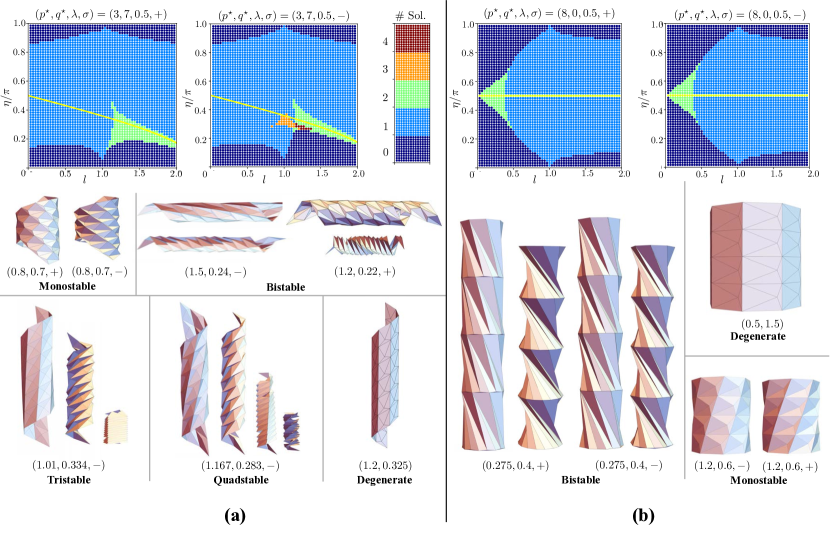
Figure 4: Phase diagrams of HMO structures parameterized by the three parameters $(l,\eta,\lambda)$ of the Miura parallelogram unit cell, as well as the mountain-valley assignment $\sigma\in\{\pm\}$. The slices of the phase diagrams displayed are taken at $\lambda=1/2$. (a) The discreteness is given by $(p^{\star},q^{\star})=(3,7)$ in this case, and the coloring scheme is in accordance to the number of HMO solutions: 0 (purple), 1 (light blue), 2 (green), 3 (orange) and 4 (red). The curve in yellow indicates a degenerate HMO that is achieved for a fully unfolded Miura parallelogram. As such, it is independent of $\lambda$ since the creases are not being utilized. Further, it always corresponds to a vertical interface. The examples below the diagrams give HMO in the different regimes of stability and are parameterized by $(l,\eta,\sigma)$, as shown. (b) An example of ring-like structures given by fixing the discreteness $(p^{\star},q^{\star})=(8,0)$. The characterization is similar.

The phase-space of HMO. The design equations above lead to a comprehensive and explicit recipe to determine all HMO:

1. Fix the reference geometry of the Miura parallelogram and chirality by assigning $(\eta,l,\lambda)$ as $0<\eta<\pi$, $l>0$ and $0<\lambda<1$, and by assigning a non-zero pair of integers $(p^{\star},q^{\star})$.

2. Assign the group parameters by the design equations in (LABEL:paramLocal-14).

3. Cycle through the folding parameter $-\pi<\omega<\pi$, $\omega\neq 0$, and solution branch $\sigma=\pm$ to numerically compute all solutions $\omega=\omega_{\star}^{\sigma}$ to the final design equation (15). This closes the cylinder and generates a HMO with the parameters $\eta,l,\lambda,p^{\star},q^{\star}$ and group parameters (LABEL:paramLocal-14) for $\omega=\omega_{\star}^{\sigma}$.

4. Cycle through the reference geometry $(\eta,l,\lambda)$ and chirality $(p^{\star},q^{\star})$ in Step 1 and repeat Steps 2 and 3 for each case to determine all HMO structures.

A natural design tool for HMO solutions is to fix the discreteness $(p^{\star},q^{\star})$ and cycle through reference parameters $(\eta,l,\lambda)$ to create a three dimensional phase diagram. In Fig. 4 below, we present two examples for illustrative purposes. These describe two-dimensional slices of such phase diagrams at $\lambda=1/2$ . In the diagrams, the coloring scheme is in accordance to the number of HMO configurations (solutions to (15)) for a fixed mountain-valley assignment ($\sigma=+$ for the left diagram and $-$ for the right diagram; Fig. 4(a) and (b), respectively). We also highlight examples of HMO in each of the respective regions.

The first phase diagram (Fig. 4(a)) is a generic helical case in which the discreteness is $(p^{\star},q^{\star})=(3,7)$. Notice the reference parameters $(l,\eta,\lambda)$ typically furnish a single HMO solution for a fixed mountain-valley assignment (light blue). However, there are regions with no solutions (purple), and regions of multistability. The $\sigma=-$ case is particularly interesting, as it has regions of bistability (green), tristability (orange) and quadstability (red). This is quite striking: by carefully designing reference parameters in the multistable regimes, the HMO achieved by such design can transform from one stable state to another by stress-induce twist and contraction (or expansion). As evidenced by the examples, the induced deformation for such transformation can be quite dramatic; for instance, the displayed tristable HMO, when deformed from its most unfolded state (denoted by folding parameter $\omega_{1}$) to its most folded state (denoted $\omega_{3}$), contracts by a factor $r_{\omega_{3}}/r_{\omega_{1}}\approx 0.7$ along its radius and by a factor $L_{\omega_{3}}/L_{\omega_{1}}\approx 0.2$ along its axial length. It also experiences $\approx 470$ degrees of twist under this transformation.

The second phase diagram (Fig. 4(b)) is for discreteness $(p^{\star},q^{\star})=(8,0)$. This characterizes ring-type HMO described by a closed ring of $8$ Miura parallelograms repeated along the axis $\mathbf{e}$ in a periodic fashion. We again see that the reference parameters $(l,\eta,\lambda)$ typically furnish a single HMO solution for a given mountain-valley assignment (light blue), but there are also regions of bistability (green). Interestingly, transformation between the two stable states in the bistable regime of parameters induces axial contraction (expansion) and twist, but no change in the radius. This means that each ring layer can be transformed independently to form a structure which is a mixture of the two different HMO states. This stands in stark contrast to the generic case $p^{\star},q^{\star}\neq 0$, where the entire structure must fully participate in the transformation from one state to the other .

Importantly, our exhaustive numerical treatment beyond these examples suggests there are no parameters for which HMO structures exhibit rigidly-foldable motions that preserve helical symmetry. However, large regions of multistability appear to be ubiquitous.

As a final comment before shifting viewpoints, we note that one drawback of this design procedure is it does not take into account self-intersection: it is actually possible for the Miura parallelogram $\mathbf{y}_{\omega}^{\sigma}(\Omega)$ and one of its neighbors $g_{1,2}(\mathbf{y}_{\omega}^{\sigma}(\Omega))$ to overlap in an unphysical way at large values of $|\omega|$ and still solve the condition (15). One such example of self-intersection is the fourth and most folded configuration (Fig. 4(a), the quadstable case). We did not exclude self-intersection in the phase diagram, as it is far too numerically laborious to do so while simultaneously exploring large regions of the configuration space. So this procedure does, in some cases, overestimate the number of stable HMO states for given set of reference parameters. Nevertheless, these self-intersecting configurations may be relevant—in the sense that, mechanistically, they suggest the possible existence of a stressed but stable mechanical equilibrium described by a tubular structure with the panels in direct contact.

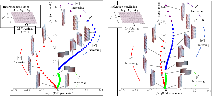
Figure 5: A diagram describing all the ways the reference tessellation, i.e., an infinite strip with width $|q^{\star}|=7$ Miura parallelogram in the top left corner, can be rolled up to form a HMO. These solve (14) and (15) for $p^{\star}=0,\ldots,150$ and $q^{\star}=7$ in blue, $p^{\star}=4,\ldots,22$ and $q^{\star}=-7$ in red, and $p^{\star}=23,\ldots,150$ and $q^{\star}=-7$ in green. The purple solutions depicted are obtained differently for aesthetic reasons: First, we solve (14) and (15) for $p^{\star}=1,2,3$ and $q^{\star}=-7$. This yields the axis orientation $\varphi=\varphi_{\star}^{\sigma}(\omega_{\star}^{\sigma})<0$. We then notice that, by replacing the axis orientation with $\varphi=\varphi_{\star}^{\sigma}(\omega_{\star}^{\sigma})+\pi$ and the discreetness $(p^{\star},q^{\star})$ with its minus, we achieve exactly the same structure. For all these solutions (blue/purple/red/green), there are also trivial solutions of mirrored chirality which correspond to $(p^{\star},q^{\star},\omega,\varphi)\mapsto-(p^{\star},q^{\star},\omega,\varphi)$. We did not bother to plot these, as they do not provide any additional information. Finally, we did not calculate the solutions beyond $|p^{\star}|=150$ since the accumulation points along the blue and green trajectories as $|p^{\star}|\rightarrow\infty$ are evident.

Now, an alternative way to view this phase-space is to fix a tessellated strip and classify all the HMO that can be obtained from this strip by the “rolling up” process (Fig. 3). For example, consider the tessellation in the top-left corner of Fig. 5. This has a width of $|q^{\star}|=7$ Miura parallelograms that are repeated along the length the strip. The boundaries of this tessellation can fit together to form a HMO in different ways; particularly, in all the ways $(p^{\star},\pm 7)$ for $p^{\star}\in\mathbb{Z}$ that solve the discreteness conditions in (14) and (15). This corresponds to different points $\mathbf{A}_{i}$ on the boundary that connect to $\mathbf{O}$ on the opposite boundary.

To clarify this viewpoint, we have completely evaluated the phase-space—in this particular sense—for the tessellation shown in Fig. 3. Strikingly, this tessellation admits a HMO solution for all $(p^{\star},\pm 7)$ and $\sigma\in\{\pm\}$, meaning that it can be isometrically rolled up to form a HMO of arbitrary chirality for either choice of mountain-valley assignment. This is highlighted graphically in Fig. 5. Starting at $p^{\star}=0$, the solutions for increasing integer values of $|p^{\star}|$ are plotted in the $(\omega,\varphi)$ phase-space. Physically, this integer increase describes a shift in the structure by one Miura parallelogram along the helical interface corresponding to the boundary of the tessellation—a process completely encapsulated by a change in both the folding parameter $\omega$ of the Miura parallelogram and axis orientation $\varphi$. We find it instructive to elaborate on this diagram in detail, as it is a natural lead-in to a mechanism for reconfigurability in HMO structures.

Briefly: For the trajectory describing increasing $|p^{\star}|$ in blue, the shift simultaneously involves widening the radius and contracting along the axis. Interestingly, the helical interface traced out by this shift is gradually flattening out as $|p^{\star}|\rightarrow\infty$. However, for reasons of discreteness, it cannot go completely flat since a horizontal interface can only exist for $p^{\star}=0$ . Instead, we see the emergence of an accumulation point (limit as $|p^{\star}|\rightarrow\infty$) at roughly $\pi^{-1}(\omega,\varphi)\approx(0,0.13)$. In contrast, the trajectory in purple is also for increasing integer values of $|p^{\star}|$, starting from zero, but describes a shift along the helical interface in the opposite sense, which takes the interface ever more vertical. This involves extension along the axis and contraction of the radius; a process that, evidently, cannot continue indefinitely. Instead, there is a transition in the chirality from $|p^{\star}|=3$ to $|p^{\star}|=4$ (purple to red) that is achieved by flipping each mountain and valley of the Miura parallelogram, as indicated by the sign change in $\omega$. After the transition, the trajectory for increasing $|p^{\star}|$ in red describes a shifting helical interface that goes evermore horizontal again, resulting in expansion of the radius and contraction along the axis. This also does not continue indefinitely, as there is a final transition between $|p^{\star}|=22$ and $|p^{\star}|=23$ (red to green) which again flips each mountain and valley of the Miura parallelogram. Along the green trajectory, we can take $|p^{\star}|\rightarrow\infty$. The shifting helical interface is flattening out giving, seemingly, the same accumulation point in the phase-space $\pi^{-1}(\omega,\varphi)\approx(0,0.13)$ as the blue trajectory, but corresponding to solutions of the opposite chirality.

Importantly, these transitions—whereby $\omega$ changes signs and induces a flip in the mountain valley assignment—occur exactly when one of the helical interfaces is nearly vertical. Our musings in this direction, guided by further numerical evidence, suggest this is an observation generic to all HMO structures. Recall that vertical interfaces correspond to the fully degenerate lines in the phase diagrams (Fig. 4), and describe HMO solutions for which the Miura parallelogram is completely unfolded (i.e., $\omega=0$). We observe that configurations“above” the line and “below” the line correspond to a change in the sign of $\omega$, and this is apparently what is happening in the transition of $|p^{\star}|=3$ to $4$ and $|p^{\star}|=22$ to $23$ in Fig 5. As a final comment related to the diagrams, it is tantalizing to think that the solutions for the two mountain-valley assignments can be directly mapped onto each other by a linear transformation in the $(\omega,\varphi)$ phase space, as it very much looks like the $\sigma=-$ solutions are related to the $+$ solutions by a contraction of the folding angle $\omega$. Alas, we have checked this carefully, and it is not the case.

In summary, we have presented a general framework to investigate the phase-space of HMO structures. Our numerical efforts in this direction suggest that rigidly foldable motions that preserve helical symmetry are impossible in such structures. Nevertheless, as the examples in Fig.4 and 5 highlight, multistability for a fixed discreteness $(p^{\star},q^{\star})$ is an ubiquitous feature, and a rich variety of configurations can generically be achieved by rolling up a reference tessellation in different ways. In what follows, we exploit these two features to discuss approaches for making these structures reconfigurable.

Motion by slip. One such means of reconfigurability is suggested by the diagram in Fig. 5: A variety of HMO are achieved from the same underlying tessellation by solving the discreteness conditions (14) and (15) for different discrete values of $p^{\star}\in\mathbb{Z}$ (with $|q^{\star}|=const.$ a fixed integer describing the number of unit cells along the width of the tessellated strip of interest). However, notice that the parameterizations also make sense when treating $p^{\star}$ as a continuous parameter and solving these equations. We simply “connect the dots” along a continuous curve in the $(\omega,\varphi)$ phase-space. While this continuation does not give a HMO for non-integer values of $p^{\star}$, it does describe a rigidly foldable isometric origami motion of this tessellation. Precisely, consider any continuous curve $(\omega_{p^{\star}}^{\sigma},\varphi_{\star}^{\sigma}(\omega_{p^{\star}}^{\sigma}))$ that solves (14-15) for $p^{\star}$ in some connected interval of $\mathbb{R}$. Substituting this curve into the group parameters (LABEL:paramLocal) and then all the parameters into (11), we observe that the deformation must describe rigidly foldable origami as a function of $p^{\star}$ due to the underlying continuity and distance preserving nature of all of these maps. In fact, there is a quite simple physical interpretation; this is nothing but motion by slip along the helical interface that connects the boundaries of the tessellation.

An example to this effect is provided in Fig. 6. For the same underlying tessellation, we vary $p^{\star}$ continuously from $2$ to $5$ to generate a continuous curve of solutions to (14) and (15) in the $(\omega,\varphi)$ phase-space. The origami structures (obtained by substituting solutions on this curve into (LABEL:paramLocal) and (11)) are displayed at integers and half-integers. Notice at the half-integers $p^{\star}=2.5,3.5,4.5$, the misfit (in red) is along a single helical interface and exactly halfway between two HMO structures $p^{\star}\pm 1/2$ (in blue). This clearly indicates motion by slip along the helical interface.

We should point out that this slip motion is by no means special to the particular example shown but rather generic to these origami structures. Thus, it would seem a natural means of reconfigurability in engineering design: For example, one could design a slider mechanism that attaches to the two boundaries of the underlying tessellation. For the design, we envision that, once the two sides are connected to form a HMO, this slider would allow for easy motion along the helical interface but would otherwise act as a linear spring for distortion in the radial direction and be (ideally) rigid for distortion normal to the radial and helical tangent directions. In this sense then, the square of the max misfit displacement (e.g., $\Delta^{2}$ for $\Delta$ in the example Fig. 6) would provide a reasonable proxy to the energy barrier to motion up to, say, a constant depending only on the design of the slider. Since the motion is otherwise rigidly foldable origami—and, particularly, involves no change in the mountain-valley assignment in most instances—it is reasonable that all other sources of energy in the system (e.g., a “bending energy” of the folds or friction in the hinges) could be made negligible by comparison. As a result, we expect such designs to achieve equilibrium states at exactly each discrete value of $p^{\star}$ that admits a HMO along a continuous path in the $(\omega,\varphi)$ phase-space. We also expect a modest energy barrier for transitioning between these discrete states. Thus, reconfigurability here would presumably involve an actuation or loading that exceeds the energy barrier; thereby, allowing the structure to “jump” from one HMO to its neighbor.

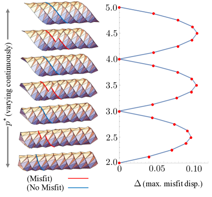
Figure 6: By treating $p^{\star}$ as a continuous parameter in the design equations, a rigidly foldable motion corresponding to slip along a helical interface is achieved (left). This induces a misfit displacement in the radial direction at the boundaries of the tessellation for non-discrete values of $p^{\star}$ (right).

Motion by phase transformation. Multistabilty is ubiquitous in mechanical systems Kebadze20042801 ; bistable_helices_00 , and one can often leverage this to obtain overall motion by transforming the system from one stable state to another. In HMO, we have a generically multistable mechanical system for a fixed discreteness due to the underlying constraints imposed by cylindrical origami; there is typically a plus-phase and minus-phase (sometimes multiple such states) corresponding to the two different mountain-valley assignments for the Miura parallelogram (Fig. 4). We exploit this feature to study coexistence of phases, i.e., whether the two phases can exist as mixtures that result in cylindrical origami, with the potential to produce overall motion. The line of thinking here is inspired by geometric compatibility in martensitic phase transformations ball_fine_1987 ; song_enhanced_2013 ; bhattacharya_microstructure_2003 and its analog for discrete helical structures feng2019phase .

To address coexistence of phases, the naive idea is to transform one of the phases generating a HMO to another via the propagation of geometrically compatible interfaces, but there is admittedly some subtlety. We begin by considering two locally compatible origami structures generated by the same underlying tessellation: $\check{\mathcal{G}}\mathbf{y}_{\check{\omega}}^{\check{\sigma}}(\Omega)=\{\check{g}_{1}^{p}\check{g}_{2}^{q}(\mathbf{y}_{\check{\omega}}^{\check{\sigma}}(\Omega))\colon(p,q)\in\mathbb{Z}^{2}\}$ and $\hat{\mathcal{G}}\mathbf{y}_{\hat{\omega}}^{\hat{\sigma}}(\Omega)=\{\hat{g}_{1}^{p}\hat{g}_{2}^{q}(\mathbf{y}_{\hat{\omega}}^{\hat{\sigma}}(\Omega))\colon(p,q)\in\mathbb{Z}^{2}\}$, where $\check{g}_{i}$ (respectively, $\hat{g}_{i}$) have group parameters as in (LABEL:paramLocal) with $(\omega,\varphi,\sigma)=(\check{\omega},\check{\varphi},\check{\sigma})$ (respectively, $(\omega,\varphi,\sigma)=(\hat{\omega},\hat{\varphi},\hat{\sigma})$) on the domain given above. Note that we are not enforcing the discreteness condition (14-15), as this will be relaxed since the origami here can involve more than one phase. In fact, by arguing rigorously in the Supplement, we show that necessary and sufficient conditions for a closed cylindrical origami of these two phases are

$$\tau_{1}^{\check{\sigma}}(\check{\omega},\check{\varphi})=\tau_{1}^{\hat{\sigma}}(\hat{\omega},\hat{\varphi}),$$ (16)

$$\theta_{1}^{\check{\sigma}}(\check{\omega},\check{\varphi})=\theta_{1}^{\hat{\sigma}}(\hat{\omega},\hat{\varphi}),$$

$$p^{\star}\tau_{1}^{\check{\sigma}}(\check{\omega},\check{\varphi})+\tilde{q}\check{\tau}_{2}^{\check{\sigma}}(\check{\omega},\check{\varphi})+(q^{\star}-\tilde{q})\tau_{2}^{\hat{\sigma}}(\hat{\omega},\hat{\varphi})=0,$$

$$p^{\star}\theta_{1}^{\check{\sigma}}(\check{\omega},\check{\varphi})+\tilde{q}\theta_{2}^{\check{\sigma}}(\check{\omega},\check{\varphi})+(q^{\star}-\tilde{q})\theta_{2}^{\hat{\sigma}}(\hat{\omega},\hat{\varphi})=2\pi,$$

for some $p^{\star},\tilde{q},q^{\star}\in\mathbb{Z}$ with $|\tilde{q}|\leq|q^{\star}|$ and $q^{\star}\tilde{q}\geq 0$. (Trivially, we can also exchange the roles of $(\cdot)_{2}$ and $(\cdot)_{1}$ above.) We focus on the system in (LABEL:twoPhase) without loss of generality.

This system of equations, when solved, admits three types of cylindrical origami depending on the values of the various parameters: HMO (i.e., single-phased cylindrical origami), those with horizontal interfaces, and those with helical interfaces. The former is obvious; if we set $(\check{\omega},\check{\varphi},\check{\sigma})=(\hat{\omega},\hat{\varphi},\hat{\sigma})$, then the system in (LABEL:twoPhase) degenerates to the original discreteness condition (8), which is solved via the procedure in (14-15). Alternatively, horizontal interfaces correspond to $q^{\star}=\tilde{q}=0$ and $(\check{\omega},\check{\varphi},\check{\sigma})\neq(\hat{\omega},\hat{\varphi},\hat{\sigma})$. Finally, helical interfaces correspond to everything else, i.e., $p^{\star},\tilde{p}\neq 0$ and $(\check{\omega},\check{\varphi},\check{\sigma})\neq(\hat{\omega},\hat{\varphi},\hat{\sigma})$. In particular, the latter two formulas for helical interfaces describe a $\rho$-averaged discreteness condition given the former two. That is, these formulas can be written as $p^{\star}\langle\tau_{1}\rangle_{\rho}+q^{\star}\langle\tau_{2}\rangle_{\rho}=0$ and $p^{\star}\langle\theta_{1}\rangle_{\rho}+q^{\star}\langle\theta_{2}\rangle_{\rho}=2\pi$ with $\rho=\tilde{q}/q^{\star}$ being the density of $\check{(\cdot)}$-phase. In this sense, we will show that $|\tilde{q}|$ and $|q^{\star}|-|\tilde{q}|$ are the number of rows of the $\check{(\cdot)}$-phase and $\hat{(\cdot)}$-phase, respectively, for this type of cylindrical origami.

Focusing first on simpler case of a horizontal interface (i.e., $q^{\star}=\tilde{q}=0$), we see that (LABEL:twoPhase) reduces to

$$\tau_{1}^{\check{\sigma}}(\check{\omega},\check{\varphi})=\tau_{1}^{\hat{\sigma}}(\hat{\omega},\hat{\varphi})=0,$$ (17)

$$p^{\star}\theta_{1}^{\check{\sigma}}(\check{\omega},\check{\varphi})=p^{\star}\theta_{1}^{\hat{\sigma}}(\hat{\omega},\hat{\varphi})=2\pi.$$

As a consequence, the complete characterization of the solutions here is rather trivial. Specifically, any set of parameters which generates a ring-type HMO (i.e., solves (14-15) with $q^{\star}=0$) can evidently be connected to any other along a horizontal interface, and these are the only types of solutions in this case. This is quite striking: As HMO solutions in this case typically come in pairs (a plus and minus phase; sometimes two each), it is a generic fact that such structures can form mixtures of the two (or four) phases along horizontal interfaces.

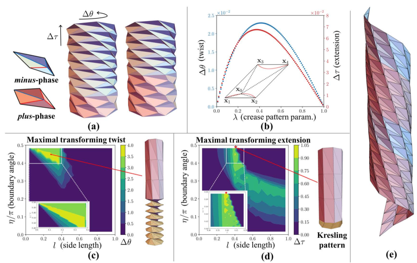
Figure 7: Phase transforming HMO. (a) Overall twist and extension obtained by transformation via a compatible horizontal interface. (b) . The twist $\Delta\theta$ and extension $\Delta\tau$ with $(l,\eta)=(1.5,\pi/4)$ for $0<\lambda<1$. (c-d) The maximal twist and extension as a function of the reference parameters $(l,\eta,\lambda)$. Each point in the phase space indicates the twist and extension after maximizing with respect to $\lambda$. For a more detailed diagram that highlights the $\lambda$ dependence, see the supplemental. (e) An example of cylindrical origami with helical interfaces.

One example, involving a change in the mountain-valley assignment for the Miura parallelograms, is provided in Fig 7(a). Notice that, when a ring is transformed, it produces an overall twist and extension of the structure: The parameters $\theta_{1}$ and $\tau_{1}$ for the generators $\check{g}_{1}$ and $\hat{g}_{1}$ are identical (as they solve (LABEL:simplePhase)), but their analogs $\theta_{2}$ and $\tau_{2}$ in $\check{g}_{2}$ and $\hat{g}_{2}$ need not be. The overall twist and extension is simply the manifestation of this difference. That is, whenever a single ring is transformed, the magnitudes of overall twist and extension are $\Delta\theta=|(\check{\theta}_{2}-\hat{\theta}_{2})|$ and $\Delta\tau=|\check{\tau}_{2}-\hat{\tau}_{2}|$, respectively .

As these quantities are often figures of merit in design, it seems quite natural to address what ring-structures ($q^{\star}=0$) give the maximal overall twist or maximal overall extension when a layer is transformed. This can be done systematically. We first fix the boundary of of Miura parallelogram. Then, as a function of the crease pattern parameter $0<\lambda<1$ defining the interior vertex, we compute the parameters that give a multistable HMO and find the maximum difference $\Delta\tau$ and $\Delta\theta$ for this $\lambda$-dependence (Fig. 7(b)). Finally, we cycle through the boundary parameters $(l,\eta)$ and repeat. The results of this procedure for $p^{\star}=8$ are highlighted graphically in Fig. 7(c-d) and are quite illuminating for design. For ring-type HMO with horizontal interfaces, we conclude:

1. The transforming twist is largest in the triangular region depicted in Fig. 7(c). These involve a twist with angle $\approx\pi$ per transforming layer.

2. The maximal extension is unambiguously achieved as $(l,\eta,\lambda)\rightarrow(0.414,\pi/2,0)$, which exactly corresponds to a special Kresling pattern.

A transformation inducing the maximal twist (i.e., on in the triangular region) and the special Kresling pattern are also provided in the figures. The latter has the feature that the Miura parallelogram—actually, the limit $\lambda\rightarrow 0$ of Miura parallelograms—generates a HMO in the completely unfolded and the fully folded-in-half states. Hence, the extension achieved is as large as can ever be expected, as it is the full height of the layer itself. The former is one of many examples for which a nearly degenerate HMO can transform along the same mountain-valley assignment, inducing a twist-per-layer that is essentially half the circumference of the cylinder.

We end the discussion of compatible interfaces by briefly introducing an example corresponding to the helical case (Fig. 7(e)). This is obtained by solving the system of equations in (LABEL:twoPhase) with $\tilde{q}=3$, $q^{\star}=8$ and $p^{\star}=8$. We do not present here a general strategy for solving this class of problems. Instead, the solution is achieved by an iterative procedure involving slight perturbations of both plus-phase and minus-phase HMO with this discreteness. Observe that the perturbed phases are such that a three layered plus-phase can connect to a five layered minus-phase in such a way to be perfectly compatible along two infinitely long helical interfaces. Additional perturbations are required to propagate the geometrically compatible helical interfaces (i.e., solve the system with different $\tilde{q}$) and induce an overall motion (twist and extension). Such change in solutions is significant, as it avoids the issue of rigidity we observed with helical interfaces of two phases in atomic structures feng2019phase .

Discussion. In this work, we have presented a thorough—if not complete—characterization of the phase-space of Helical Miura Origami. The results are mostly explicit and quantitative, but otherwise involve only the simplest of numerical implementation. As such, this characterization should make for an efficient design tool for the myriad of applications seeking multi-functional and tunable structures: The motion by slip, which induces expansion (or contraction) radially in the structure, would seem a natural mechanism in the design of medical stents. The quadstable ring structures—really their “fold-in-half” analogs—are already being explored as a concept for deployable space structures ftp_PNAS_2015 . And the helical symmetry, which is on full display in this methodology, has the potential to be exploited for the design of novel electro-magnetic antennas ; particularly, since discrete symmetries can interact with Maxwell’s equations to produce highly directionalized electro-magnetic profiles jfj_actacryst_16 . In fact, the helical interfaces are an interesting example in this setting, as they involve both a short-wavelength helical symmetry (the unit cell) and a long-wavelength symmetry (e.g., a shift and potential twist of the eight layers along the axis in Fig 7(e)).

On the theoretical front, the abstraction underlying all the results here is: discrete and Abelian groups of isometries interact naturally with origami unit cells to produce complex—hopefully interesting—structures. While we have chosen to focus our attention on one type of unit cell (the Miura parallelogram), the approach applies much more broadly. For instance, Kawasaki’s condition can certainly be relaxed paul_miura and still yield an origami unit cell. In addition, advances in 3-D/4-D printing and manufacturing make it sensible to also consider: 1) origami that is absent a flat configuration, and 2) simple building blocks of nonisometric origami plucinsky_actuation_2018 ; plucinsky2018patterning made of active materials. In all such cases, as long as the unit cell has four and only four corners, the design equations for the group parameters (i.e., the equations (LABEL:paramLocal-15)) directly apply to construct any Helical Origami. Thus, the group theoretic approach to origami design would seem to have a broad and remarkable scope.

Acknowledgment. The authors gratefully acknowledge the support of the Air Force Office of Scientific Research through the MURI grant no. FA9550-16-1-0566.

References

- (1) F. Feng, P. Plucinsky, and R. D. James, “Phase transformations and compatibility in helical structures,” Journal of the Mechanics and Physics of Solids, 2019.
- (2) E. A. Peraza-Hernandez, D. J. Hartl, R. J. Malak Jr, and D. C. Lagoudas, “Origami-inspired active structures: a synthesis and review,” Smart Materials and Structures, vol. 23, no. 9, p. 094001, 2014.
- (3) L. Wilson, S. Pellegrino, and R. Danner, “Origami sunshield concepts for space telescopes,” in 54th AIAA/ASME/ASCE/AHS/ASC Structures, Structural Dynamics, and Materials Conference, p. 1594, 2013.
- (4) M. Schenk, S. Kerr, A. Smyth, and S. Guest, “Inflatable cylinders for deployable space structures,” in Proceedings of the First Conference Transformables, Sept, pp. 18–20, 2013.
- (5) P. M. Reis, F. L. Jiménez, and J. Marthelot, “Transforming architectures inspired by origami,” Proceedings of the National Academy of Sciences, vol. 112, no. 40, pp. 12234–12235, 2015.
- (6) T. Tachi and G. Epps, “Designing one-dof mechanisms for architecture by rationalizing curved folding,” in International Symposium on Algorithmic Design for Architecture and Urban Design (ALGODE-AIJ). Tokyo, 2011.
- (7) S. Waitukaitis, R. Menaut, B. G.-g. Chen, and M. van Hecke, “Origami multistability: From single vertices to metasheets,” Physical review letters, vol. 114, no. 5, p. 055503, 2015.
- (8) S. Waitukaitis and M. van Hecke, “Origami building blocks: Generic and special four-vertices,” Physical Review E, vol. 93, no. 2, p. 023003, 2016.
- (9) B. G.-g. Chen, B. Liu, A. A. Evans, J. Paulose, I. Cohen, V. Vitelli, and C. Santangelo, “Topological mechanics of origami and kirigami,” Physical review letters, vol. 116, no. 13, p. 135501, 2016.
- (10) J. A. Faber, A. F. Arrieta, and A. R. Studart, “Bioinspired spring origami,” Science, vol. 359, no. 6382, pp. 1386–1391, 2018.
- (11) P. W. K. Rothemund, “Folding dna to create nanoscale shapes and patterns,” Nature, vol. 440, pp. 297 EP –, 03 2006.
- (12) D. Han, S. Pal, J. Nangreave, Z. Deng, Y. Liu, and H. Yan, “Dna origami with complex curvatures in three-dimensional space,” Science, vol. 332, no. 6027, pp. 342–346, 2011.
- (13) X. Liu, S. Yao, S. V. Georgakopoulos, B. S. Cook, and M. M. Tentzeris, “Reconfigurable helical antenna based on an origami structure for wireless communication system,” in 2014 IEEE MTT-S International Microwave Symposium (IMS2014), pp. 1–4, June 2014.
- (14) S. Yao, X. Liu, S. V. Georgakopoulos, and M. M. Tentzeris, “A novel reconfigurable origami spring antenna,” in Antennas and Propagation Society International Symposium (APSURSI), 2014 IEEE, pp. 374–375, IEEE, 2014.
- (15) M. Schenk and S. D. Guest, “Geometry of miura-folded metamaterials,” Proceedings of the National Academy of Sciences, vol. 110, no. 9, pp. 3276–3281, 2013.
- (16) H. Yasuda and J. Yang, “Reentrant origami-based metamaterials with negative poisson’s ratio and bistability,” Physical review letters, vol. 114, no. 18, p. 185502, 2015.
- (17) J. L. Silverberg, A. A. Evans, L. McLeod, R. C. Hayward, T. Hull, C. D. Santangelo, and I. Cohen, “Using origami design principles to fold reprogrammable mechanical metamaterials,” science, vol. 345, no. 6197, pp. 647–650, 2014.
- (18) Z. Y. Wei, Z. V. Guo, L. Dudte, H. Y. Liang, and L. Mahadevan, “Geometric mechanics of periodic pleated origami,” Physical review letters, vol. 110, no. 21, p. 215501, 2013.
- (19) E. T. Filipov, T. Tachi, and G. H. Paulino, “Origami tubes assembled into stiff, yet reconfigurable structures and metamaterials,” Proceedings of the National Academy of Sciences, vol. 112, no. 40, pp. 12321–12326, 2015.
- (20) L. H. Dudte, E. Vouga, T. Tachi, and L. Mahadevan, “Programming curvature using origami tessellations,” Nature materials, vol. 15, no. 5, p. 583, 2016.
- (21) K. Miura, “Concepts of deployable space structures,” International Journal of Space Structures, vol. 8, no. 1-2, pp. 3–16, 1993.
- (22) P. Plucinsky, F. Feng, and R. D. James, “The design and deformations of generalized miura origami,” preprint.
- (23) J. C. Bowers and I. Streinu, “Lang’ s universal molecule algorithm,” Annals of Mathematics and Artificial Intelligence, vol. 74, no. 3-4, pp. 371–400, 2015.
- (24) R. J. Lang and L. Howell, “Rigidly foldable quadrilateral meshes from angle arrays,” Journal of Mechanisms and Robotics, vol. 10, no. 2, p. 021004, 2018.
- (25) K. Wang and Y. Chen, “Folding a patterned cylinder by rigid origami,” Origami, vol. 5, pp. 265–276, 2011.
- (26) F. Bös, M. Wardetzky, E. Vouga, and O. Gottesman, “On the Incompressibility of Cylindrical Origami Patterns,” Journal of Mechanical Design, vol. 139, pp. 021404–021404–9, Dec. 2016.
- (27) C. Jianguo, D. Xiaowei, Z. Ya, F. Jian, and T. Yongming, “Bistable behavior of the cylindrical origami structure with kresling pattern,” Journal of Mechanical Design, vol. 137, no. 6, p. 061406, 2015.
- (28) T. Tachi, “Generalization of rigid foldable quadrilateral mesh origami,” in Symposium of the International Association for Shell and Spatial Structures (50th. 2009. Valencia). Evolution and Trends in Design, Analysis and Construction of Shell and Spatial Structures: Proceedings, Editorial Universitat Politècnica de València, 2009.
- (29) R. D. James, “Objective structures,” Journal of the Mechanics and Physics of Solids, vol. 54, no. 11, pp. 2354–2390, 2006.
- (30) M. Dresselhaus, G. Dresselhaus, and R. Saito, “Physics of carbon nanotubes,” Carbon, vol. 33, no. 7, pp. 883–891, 1995.
- (31) R. D. James, “Symmetry, invariance and the structure of matter,” in Proceedings of the International Congress of Mathematicians 2018 (ICM 2018), World Scientific, 2019.
- (32) E. Kebadze, S. Guest, and S. Pellegrino, “Stable prestressed shell structures,” International Journal of Solids and Structures, vol. 41, no. 11–12, pp. 2801 – 2820, 2004.
- (33) R. E. Goldstein, A. Goriely, G. Huber, and C. W. Wolgemuth, “Bistable helices,” Physical review letters, vol. 84, no. 7, p. 1631, 2000.
- (34) J. M. Ball and R. D. James, “Fine phase mixtures as minimizers of energy,” Archive for Rational Mechanics and Analysis, vol. 100, no. 1, pp. 13–52, 1987.
- (35) Y. Song, X. Chen, V. Dabade, T. W. Shield, and R. D. James, “Enhanced reversibility and unusual microstructure of a phase-transforming material,” Nature, vol. 502, pp. 85–88, Oct. 2013.
- (36) K. Bhattacharya, Microstructure of martensite : why it forms and how it gives rise to the shape-memory effect. Oxford: Oxford University Press, 2003.
- (37) D. Jüstel, G. Friesecke, and R. D. James, “Bragg–von laue diffraction generalized to twisted x-rays,” Acta Crystallographica Section A: Foundations and Advances, vol. 72, no. 2, pp. 190–196, 2016.
- (38) P. Plucinsky, M. Lemm, and K. Bhattacharya, “Actuation of Thin Nematic Elastomer Sheets with Controlled Heterogeneity,” Archive for Rational Mechanics and Analysis, vol. 227, pp. 149–214, Jan. 2018.
- (39) P. Plucinsky, B. A. Kowalski, T. J. White, and K. Bhattacharya, “Patterning nonisometric origami in nematic elastomer sheets,” Soft matter, vol. 14, no. 16, pp. 3127–3134, 2018.