Fractional Operators Applied to Geophysical Electromagnetics

Abstract

A growing body of applied mathematics literature in recent years has focussed on the application of fractional calculus to problems of anomalous transport. In these analyses, the anomalous transport (of charge, tracers, fluid, etc.) is presumed attributable to long–range correlations of material properties within an inherently complex, and in some cases self-similar, conducting medium. Rather than considering an exquisitely discretized (and computationally intractable) representation of the medium, the complex and spatially correlated heterogeneity is represented through reformulation of the PDE governing the relevant transport physics such that its coefficients are, instead, smooth but paired with fractional–order space derivatives. Here we apply these concepts to the scalar Helmholtz equation and its use in electromagnetic interrogation of Earth’s interior through the magnetotelluric method. We outline a practical algorithm for solving the Helmholtz equation using spectral methods coupled with finite element discretization. Execution of this algorithm for the magnetotelluric problem reveals several interesting features observable in field data: long–range correlation of the predicted electromagnetic fields; a power–law relationship between the squared impedance amplitude and squared wavenumber whose slope is a function of the fractional exponent within the governing Helmholtz equation; and, a non–constant apparent resistivity spectrum whose variability arises solely from the fractional exponent. In geologic settings characterized by self–similarity (e.g. fracture systems; thick and richly–textured sedimentary sequences, etc.) we posit that diagnostics are useful for geologic characterization of features far below the typical resolution limit of electromagnetic methods in geophysics.

1 Introduction

Anomalous diffusion has been at the heart of considerable research directed at understanding non-standard, or “anomalous”, transport behavior where the mean squared displacement of random walk particles no longer adhere to a linear relationships with time. As a result, such systems reveal power laws indicative of sub and super-diffusive behavior. Anomalous diffusion can be described through random walks endowed by heavy tail distributions and is captured through non-integer exponents on time and space derivatives. Fractional derivatives in space model super-diffusion and are related to long power-law particle jumps, whereas fractional derivatives on temporal derivatives model sub-diffusion that are induced through long waiting times between particle jumps. Such behavior has been observed in many applications including reaction-diffusion, quantum kinetics, flow through porous media, plasma transport, magnetic fields, molecular collisions, and geophysics applications. We refer the reader to Metzler and Klafter [23] for a detailed description of anomalous diffusion, including a comprehensive list of applications. The underlying cause for anomalous behavior in these applications is the presence of complex structures or mechanisms that either promote sub-diffusion or super-diffusion. For instance, in fluid flow through porous media, complex permeability fields cause sub-diffusive transport through trapping mechanisms or solid/liquid surface-chemistry kinetics, ultimately inducing a memory–type effect [12, 14]. Super-diffusive responses have been experimentally observed in diffusion-reaction system where the variance of a chemical wave exceeds a linear temporal relationship [29]. This is interpreted to be a result of non-local interactions over distances beyond that to the nearest neighbors. In the diffusion-reaction case, vortices in a chaotic velocity field introduce flow paths that exceed standard diffusion rates.

A range of natural phenomena can be described as processes in which a physical quantity is constantly undergoing small, random fluctuations. Such Brownian motion can be interpreted as a random walk that, according to the central limit theorem, approaches a normal distribution as the number of steps increases. A macroscopic manifestation of Brownian motion is defined as diffusion whereby a collection of microscopic quantities tends to spread steadily from regions of high concentration to regions of lower concentration. Through Fick’s first and second laws, macroscopic particle movement can be captured by the familiar diffusion equation, the solution of which is identical to a normal distribution and corresponds to the random walk probability density. These well known concepts provide the underpinning to investigate phenomena that violate the standard diffusive regime. An application space which has received relatively little attention but is poised for further exploration is low-frequency electromagnetic imaging and interrogation of Earth’s subsurface, a classic geophysical exploration technique premised on diffusive (transport) physics, either through the mobility of solid-state defects in crystalline materials and free electrons in metals, or electrolytic conduction in fluids [19].

Capturing anomalous diffusion in partial differential equations poses considerable mathematical and numerical challenges, in particular in the area of 1) imposing non-zero boundary conditions, 2) validating fractional behavior for different physics, and 3) achieving computational efficiency to realize scalable performance. To solve the fractional Laplacian an integral or a spectral definition can be considered. The choice of method however remains an open question, in particular for non-zero boundary conditions. In this paper we consider the spectral definition and justify this choice based on the authors’ previous developments. Validating fractional PDEs against field observations, laboratory measurement, or analytic solutions is difficult, in part, because fractional calculus development has been somewhat isolated from engineering and science applications community. In this paper, we offer results to help bridge that gap between the observational science and mathematics communities. In particular, fractional concepts are applied to geophysical electromagnetics to better characterize the subsurface and subsequently validated through field observations, as well as geophysical insight. A key challenge in simulating fractional PDEs is achieving computational efficiency. In our work we pursue an approach that leverages the Dunford–type integral representation which, in the case of fractional Laplacians, is computationally very attractive because of an embarrassingly parallel loop for solving multiple Laplacians. This parallelism however does not map to our Helmholtz implementation because of coupling cross-terms, a fact which impacts our eventual desire to make use of adjoint-based optimization. Nonetheless, we begin with Bonito and Pasciak’s solution strategy [10, 9], with its resultant Helmholtz coupling, and augment it with the lifting (splitting) strategy of Antil [3] for handling non-zero boundary conditions to arrive at a unique approach to solving the fractional Helmholtz equation, regardless of its particular application here in geophysical electromagnetics.

The aim of this paper is to explore anomalous diffusion in the context of geophysical electromagnetics and to derive mathematical and algorithmic strategies for practical simulation capabilities. Subsurface geology can exhibit complex features ranging from hierarchical structures to self-similar geometries. Electromagnetic energy exposed to such media will likely produce signals significantly different from homogenous and isotropic media. For example, non-local electromagnetic effects have been observed in near-surface, geotechnical engineering settings as a result of complex structured conductivity in the subsurface [17, 30, 18]. Other phenomena in the subsurface have been demonstrated in the context of fluid flow in porous media and would have equivalent non-local effects on geophysical electromagnetics [12, 14, 7]. Fractured systems have been reported to be linked to non-local effects [30, 18], as well as layered media [15]. We are interested in detecting small scale features in the geological subsurface (e.g. fine-scale stratigraphic laminations or regions permeated by fractures) that aggregate into a hierarchical “meta-material” while also, by practical necessity, avoiding the detailed and computationally explosive discretization required to represent each of them in a given numerical simulation. Following Caputo’s strategy of replacing the standard scalar permeability and gradient combinations in Darcy’s law with a fractional derivative [12], we replace the Ohm’s empirical relationship with a fractional derivative to arrive at a fractional Helmholtz equation.

Our main contributions consist of 1) deriving fractional Helmholtz via Ampere’s law by introducing a fractional spatial differential operator into Helmholtz to account for non-local conductivity; the solution process of this fractional partial differential equation (PDE) requires a decomposition to separate boundary conditions from the fractional Laplacian operator; 2) implementing computationally efficient methods through a combination of spectral characterization of the Laplacian, finite element discretization, and a Dunford–type integral representation; a reformulation allows for sparse Jacobians and a scaling adjustment provides for a much improved conditioning; 3) validating EM behavior through magnetotullerics. The remainder of the paper is organized by first deriving the fractional Helmholtz equation through a fractional gradient relationship between the magnetic field and the underlying electric conductivity. Next the fractional Helmholtz equation with non-zero boundary conditions is decomposed to separate non-zero right-hand side and non-zero boundary conditions. The separation provides a convenient solution strategy and leverages the Dunford–type integral approach to numerically solve one of the remaining equations with a fractional Laplacian. After the mathematical formulation, our finite element implementation is verified through the methods of manufactured solutions. Finally, our numerical capability is demonstrated on a relevant magnetotullerics application. Our numerical results are validated through field measurements and geophysical insight.

2 Mathematical Formulation

The formulation that follows consists of multiple steps. We start by motivating the fractional derivative operator in the context of geophysical electromagnetics and define Ohm’s constitutive law in terms of a fractional space derivative, later moving that derivative to the Laplacian term of the Helmholtz PDE. Given a fractional Helmholtz equation with non-zero boundary conditions, a two-equation decomposition provides a grouping of boundary conditions, source terms, and fractional operators that allow for convenient solution strategies. One equation with non-homogeneous boundary conditions is transformed to non-fractional form by deriving the “very weak form” so that standard solution techniques can be applied. For the remaining equation with a fractional Laplacian and homogeneous boundary conditions, we appeal to a spectral representation and resolvent formalism whereby the fractional Laplacian is transformed to a summation of standard Laplacians using a Dunford–type integral with appropriate quadrature. The solution to the final system of equations is detailed in section (3) in which a finite element discretization of both equations results in a large and dense coefficient matrix that requires further manipulation to achieve efficient solution performance.

We start with Faraday’s law in the frequency domain with the Fourier convention of time derivatives $\partial_{t}$ mapping to the frequency domain $\omega$ as $\partial_{t}\mapsto\text{i}\omega$ and assuming constant magnetic permeability $\mu_{0}=4\pi\times 10^{-7}$ H/m:

$$\nabla\times\mathbb{E}=-\text{i}\omega\mu_{0}\mathbb{H},$$ (1)

relating the curl of electric field $\mathbb{E}$ to time variations in magnetic field $\bf H$. Paired with this is Ampère’s Law, $\nabla\times\mathbb{H}=\mathbb{J}$, where $\mathbb{J}$ is the total electric current density: The sum of Ohmic currents; Maxwell’s discplacement current $\text{i}\omega\varepsilon\mathbb{E}$; and, any impressed external currents due to antennas and electrodes. Typically, for simple linear, isotropic materials the Ohmic currents are described by the product of electrical conductivity $\sigma$ and electric field and at suffiently low frequencies $\sigma>>\omega\varepsilon$ Maxwell’s displacement current can safely be ignored. In a similar fashion as Caputo [12] in which he replaced the permeability in Darcy’s equation with a time–fractional derivative, we replace the simple conductivity/field product in Ohm’s law with a space–fractional derivative. Preserving the symmetry of both positive and negative power law jumps in the $z$ direction for a two–sided stable diffusion process requires both positive and negative fractional derivatives [22, p15] $\mathcal{D}^{\alpha}_{z}={1\over 2\cos({1\over 2}\pi\alpha)}{\left({\partial^{\alpha}\over{\partial z^{\alpha}}}+{\partial^{\alpha}\over\partial(-z)^{\alpha}}\right)}$ which we normalize by the factor $\cos({1\over 2}\pi\alpha)$ to preserve magnitude invariance under $\alpha$. As a consequence, the space–Fourier transform for this operator maps to the wavenumber $\nu$ domain as $D_{z}^{\alpha}\mapsto|\nu|^{\alpha}$. Note that had a one–sided derivative with Fourier mapping $(\pm\text{i}\nu)^{\alpha}$ been used, the unit–magnitude prefactor $(\pm\text{i})^{\alpha}$ could be interpreted as rotating the electrical conductivity into the complex plane, effectively reintroducing the Maxwell displacement current and turning the Maxwell derivation into a mixed diffusion/wave propagation problem rather than a strictly diffusive one. Unlike Caputo’s attempt to emulate memory effects in permeability, our hypothesis is that certain non-local conductivity properties create superdiffusive behavior and can be represented by a spatial fractional derivative. With this fractional Ohm’s law in the low–frequency limit (and no external sources) inserted into Ampère’s law, the curl of (1) is thereby:

$$\nabla\times\nabla\times\mathbb{E}=-\text{i}\omega\mu_{0}\mathcal{D}_{z}^{\alpha}\left[\sigma_{\alpha,z}\mathbb{E}\right],$$ (2)

where $\mathcal{D}_{z}^{\alpha}$ is the $\alpha$–order fractional derivative in the $z$ direction and $\sigma_{\alpha,z}$ is the electrical conductivity in units of S/m^1-α. For an Earth model whose conductivity varies only as a function of vertical coordinate $z$, subject to a vertically incident electric field oriented in the horizontal $x$ direction, the electric fields in the Earth are everywhere horizontal such that $\mathbb{E}=\hat{x}\,u(z)$ is the primary state variable that needs further consideration. Furthermore, for dimensional consistency in the fractional calculus methodology described in the following section, we non–dimensionalize with respect to the $z$ coordinate such that $z\mapsto\zeta=z/z^{*}$ to arrive at

$$-{\text{d}^{2}u\over\text{d}\zeta^{2}}\left({1\over z^{*}}\right)^{2}+\text{i}\omega\mu_{0}\mathcal{D}_{\zeta}^{\alpha}\left[\sigma_{\alpha,\zeta}\,u(\zeta)\right]=0$$ (3)

which, after action by $\mathcal{D}_{\zeta}^{-\alpha}$ and generalization to 3D, becomes

$$\left(-\Delta_{\zeta}\right)^{s}u+\text{i}\kappa^{2}\,u(\zeta)=0,$$ (4)

where $\left(-\Delta_{\zeta}\right)^{s}$ is the fractional–order Laplacian in dimensionless coordinate $\zeta$, $s=1-{1\over 2}\alpha$ and $\kappa^{2}$ the dimensionless squared wavenumber $\omega\mu_{0}\sigma_{\alpha,\zeta}\left(z^{*}\right)^{2}$. Note that in Eq (3) the conductivity $\sigma_{\alpha,z}$ possesses fractional length dimensions to retain consistency with the fractional derivative operator $\mathcal{D}_{z}^{\alpha}$. However, through the non-dimensionalization process transforming Eq (3) to Eq (4) we see that the conductivity $\sigma_{\alpha,\zeta}$ reclaims its familiar, integer-ordered units of S/m, thus avoiding awkward, fractional–dimensioned conductivities reported elsewhere [16, 18].

We observe that the fractional exponent is on the Laplacian term and in combination with the Helmholtz term motivate the challenge of a solution strategy. An additional complication is the need to incorporate non-trivial boundary conditions, such as special radiation or self-absorbing boundary conditions. We address these issues through the use of linear decomposition, a Dunford type integral formulation and the very weak form for finite element discretizations. We write the generalized fractional–order Helmholtz equation as

$$\left(-\Delta\right)^{s}u-k^{2}u =f\quad\mbox{in}\,\,\Omega,$$ (5)

$$u =g\quad\mbox{on}\,\,\Gamma,$$

where $k^{2}=-\text{i}\kappa^{2}$ is introduced to simplify notation for our electromagnetic problem, but in fact, transcends this particular choice of physics, and $(-\Delta)^{s}$ is understood to be the spectral fractional Laplacian operator for non–zero Dirichlet boundary conditions

$$\left(-\Delta\right)^{s}u(\bm{x}):=\sum_{k=1}^{\infty}\left(\lambda_{k}^{s}\int_{\Omega}u\,\varphi_{k}\,{\text{d}}\Omega+\lambda_{k}^{s-1}\int_{\Gamma}u\,\partial_{n}\varphi_{k}\,{\text{d}}\Gamma\right)\varphi_{k}(\bm{x}),$$ (6)

where $\varphi_{k}$ are the eigenfunctions of the Laplacian with corresponding eigenvalues $\lambda_{k}$ [3, Def. 2.3] and $\bm{x}\in\Omega$ is the coordinate of interest. Moreover, $u$ is assumed to be sufficiently smooth. As it is customary in the PDE theory, we have stated this definition for smooth functions, however by standard density arguments it immediately extends to Sobolev spaces, we refer to [3] for details. In addition, we emphasize that when $u=0$ on the boundary $\Gamma$, the definition above is nothing but the standard spectral fractional Laplacian $(-\Delta_{0})^{s}$ with zero boundary conditions. We will omit the subscript 0 when it is clear from the context.

Following this earlier work on fractional Poisson equation, we extend the basic approach to fractional Helmholtz and break $u$ into two parts thusly: Let $v$ solve

$$\left(-\Delta\right)^{s}v-k^{2}\left(v+w\right) =f\quad\mbox{in}\,\,\Omega,$$ (7)

$$v =0\quad\mbox{on}\,\,\Gamma,$$

and let $w$ solve

$$\left(-\Delta\right)^{s}w =0\quad\mbox{in}\,\,\Omega,$$ (8)

$$w =g\quad\mbox{on}\,\,\Gamma.$$

Summing (7) and (8) it is evident that $u=v+w$. The presence of the homogeneous boundary condition on (7) allows for a spectral representation of the Dirichlet fractional–power Laplacian operator. Furthermore, it has been shown [3] that solving (8) is equivalent to solving the standard, integer–power Laplacian equation in the very–weak sense [8, 21, c.f.], which in the case of smooth $g$ is simply the more–familiar weak sense. A simple algebraic manipulation of the spectral decomposition provides a Laplacian with integer exponents (see Theorem 4.1 and the subsequent proof in [3] for additional details). Hence, we may replace (8) with the following:

$$\left(-\Delta\right)w =0\quad\mbox{in}\,\,\Omega,$$ (9)

$$w =g\quad\mbox{on}\,\,\Gamma,$$

which, when solved simultaneously with (7), yields the solution to the original equation (5).

To solve equation (7), we follow others [10, 2, e.g.] in using spectral analysis of linear operators and resolvent formalism. Specifically, we start with Kato’s definition of fractional powers for linear operators ([20] Theorem 2 and supporting proof) and simplify by setting Kato’s $\lambda$ coefficient to zero. This definition due to Kato coincides with (6) when the function values are zero on the boundary, as in this case the surface integral over $\Gamma$ vanishes which is indeed the case in (7). The Kato’s definition after applying a variable transformation that results in a symmetric integral, which is approximated through quadrature is:

$$\left(-\Delta\right)^{-s} ={\sin s\pi\over\pi}\int_{-\infty}^{\infty}e^{(1-s)y}\left(e^{y}-\Delta\right)^{-1}\,{\text{d}}y,$$ (10)

$$\approx{\sin s\pi\over\pi}m\sum_{\ell=-N^{-}}^{N^{+}}e^{(1-s)y_{\ell}}\left(e^{y_{\ell}}-\Delta\right)^{-1},$$

where the quadrature nodes are distributed uniformly as $y_{l}=m\ell$. Accuracy of the quadrature representation of this continuous integral is a function of the constants $m$, $N^{-}$ and $N^{+}$ and has been shown to be exponentially convergent [10]. The constants are chosen such that the quadrature error is balanced with the error in the spatial discretization of (7) [10, c.f. when $w=0$]. In the case of a finite element solution with linear nodal basis functions on the unit interval and node spacing $h$, they are

$$m={1\over\ln{1\over h}},\quad N^{+}=\Big{\lceil}{\pi^{2}\over 4s\,m^{2}}\Big{\rceil},\quad\text{and}\quad N^{-}=\Big{\lceil}{\pi^{2}\over 4(1-s)\,m^{2}}\Big{\rceil}.$$ (11)

The use of the “ceiling” operators $\lceil\cdot\rceil$ in (11) ensure $N^{-}$ $N^{+}$ are integer valued, as required.

Remark 1.

In using (10), we avoid the costly (and in many cases, inaccurate) precalculation of the eigenspectrum for the Laplacian over an arbitrary spatial domain $\Omega$ with Dirichlet condition $u|_{\Gamma}=g$. Even in cases where calculation of the eigenspectrum bears an acceptable computational cost, there still remains the outstanding question of just how much of the spectrum is required for computing the Laplacian by this method to acceptable accuracy. For these reasons, our equation (10) is far more practical.

Rewriting (7) as $v-\left(-\Delta\right)^{-s}\,k^{2}(v+w)=\left(-\Delta\right)^{-s}f$, we may write $v$ as a Kato–style expansion

$$v={\sin s\pi\over\pi}m\sum_{\ell=-N^{-}}^{N^{+}}e^{(1-s)y_{\ell}}v_{\ell}$$ (12)

and equate each of the $\ell$ terms to arrive at the coupled equation

$$v_{\ell}-\left(e^{y_{\ell}}-\Delta\right)^{-1}\,k^{2}\left(v+w\right)=\left(e^{y_{\ell}}-\Delta\right)^{-1}f,$$ (13)

or

$$\left(e^{y_{\ell}}-\Delta\right)v_{\ell}-k^{2}\left(v+w\right)=f.$$ (14)

Observe that there are $N^{-}+N^{+}+1$ of these equations and that the $\ell$th equation fully couples the function $v_{\ell}$ into $w$ and all remaining functions $v_{\ell^{\prime}\neq\ell}$ of the expansion (12). Enforcement of the modified boundary condition $v_{\ell}=0$ guarantees enforcement of $v=0$ via (12). Hence, with the inclusion of (9), we have the complete differential problem statement consisting of a coupled system of $N^{-}+N^{+}+2$ equations with unknown functions $v_{N^{-}},\ldots,v_{N^{+}},w$ over the domain $\Omega$.

3 Numerical Implementation

The method of solution for equations (9) and (14) (including corresponding boundary conditions) is to first transform the differential problem statement into an equivalent variational problem statement for the appropriate infinite dimensional function spaces and then approximate its solution by the optimal one, in a Sobolev norm sense, taken from finite dimensional space of linear, nodal finite elements over some discretization. In doing so, we introduce the test function $\xi_{\ell}$ and construct the weak form of (14) for all $\ell$ from $-N^{-}$ to $N^{+}$:

$$\int_{\Omega}\left(-\xi_{\ell}\,\Delta v_{\ell}+e^{y_{\ell}}\,\xi_{\ell}v_{\ell}-k^{2}\,\xi_{\ell}\left(v+w\right)\right)\,{\text{d}}\Omega=\int_{\Omega}\xi_{\ell}f\,{\text{d}}\Omega,$$ (15)

recalling that $v$ is given by the expansion (12). The test function $\zeta$ is used in the weak form of the Laplace equation (9) as,

$$\int_{\Omega}\nabla\zeta\cdot\nabla w\,{\text{d}}\Omega=0.$$ (16)

Combining the left hand sides of (15) and (16), the bilinear form $A(\cdot,\cdot)$ is therefore given as

$$A(\left\{\xi_{\ell}\right\},\zeta;\left\{v_{\ell}\right\},w)=\sum_{\ell=-N^{-}}^{N^{+}}\int_{\Omega} \left(\nabla\xi_{\ell}\cdot\nabla v_{\ell}+e^{y_{\ell}}\,\xi_{\ell}v_{\ell}-k^{2}\,\xi_{\ell}\left(v+w\right)\right)\,{\text{d}}\Omega$$ (17)

$$+\int_{\Omega}\nabla\zeta\cdot\nabla w\,{\text{d}}\Omega,$$

the combined right hand sides are denoted as

$$F\left(\left\{\xi_{\ell}\right\},\zeta\right)=\sum_{\ell=-N^{-}}^{N^{+}}\int_{\Omega}\xi_{\ell}f\,{\text{d}}\Omega,$$ (18)

and $v$ is understood to be expanded in terms of $v_{\ell}$ according to (12). The variational problem statement equivalent to the differential problem statement in (9) and (14) is therefore: Find $\left\{v_{\ell}\right\}\in V_{0};w\in V$, such that

$$A(\left\{\xi_{\ell}\right\},\zeta;\left\{v_{\ell}\right\},w)=F\left(\left\{\xi_{\ell}\right\},\zeta\right)\quad\forall\left\{\xi_{\ell}\right\},\zeta\in V_{0},$$ (19)

where $V$ is the space of $L^{2}$ functions on $\Omega$ with first order weak derivatives also in $L^{2}$ of $\Omega$ and inhomogeneous Dirichlet boundary conditions (8), and $V_{0}\subset V$ taking homogeneous boundary conditions as in (7). The next step is to choose a finite–dimensional space $V_{h}\subset V$ from which the approximate solutions $v_{h}\approx v$ and $w_{h}\approx w$ will be drawn. To further simplify notation we will drop the $h$ subscript and only re–introduce it as needed in relation to the true (weak) solutions $v$ and $w$.

Let $\phi_{1}(\bm{x}),\phi_{2}(\bm{x}),\ldots,\phi_{N}(\bm{x})$ be the basis functions in $V_{h}$ as a function of spatial coordinate $\bm{x}$, which in our implementation will be linear, nodal finite elements . We write in bold the column vector $\bm{\phi}$ of basis functions $(\phi_{1},\phi_{2},\ldots,\phi_{N})^{T}$, and $\bm{v}_{\ell}=\left(v_{\ell}^{1},v_{\ell}^{2},\ldots,v_{\ell}^{N}\right)^{T}$. By construction, it follows that $v_{\ell}(\bm{x})=\bm{\phi}^{T}\bm{v}_{\ell}=\sum_{i=1}^{N}\phi_{i}(\bm{x})v_{\ell}^{i}$. Likewise, $\bm{\xi}_{\ell}=\left(\xi_{\ell}^{1},\xi_{\ell}^{2},\ldots,\xi_{\ell}^{N}\right)^{T}$ and $\bm{w}=\left(w_{1},w_{2},\ldots,w_{N}\right)^{T}$ yield $\xi_{\ell}=\bm{\xi}_{\ell}^{T}\bm{\phi}$ and $w=\bm{\phi}^{T}\bm{w}$, respectively. As such, construction of the linear system (19) requires the following block matrices built by volume integration of the basis functions and their spatial derivatives:

$${\mathbb{K}}=\int_{\Omega}\left(\nabla\bm{\phi}\right)^{T}\left(\nabla\bm{\phi}\right)\,{\text{d}}\Omega,\quad{\mathbb{M}}_{1}=\int_{\Omega}\bm{\phi}\bm{\phi}^{T}\,{\text{d}}\Omega,\quad\mbox{and}\quad{\mathbb{M}}_{2}=-\int_{\Omega}k^{2}\,\bm{\phi}\bm{\phi}^{T}\,{\text{d}}\Omega$$ (20)

where the integrands are understood to be outer products, each yielding a symmetric matrix of dimension $N\times N$. To simplify notation, introduce the coefficients $c_{\ell}=e^{y_{\ell-N^{-}}}$ and $d_{\ell}={1\over\pi}(\sin s\pi)\,m\,e^{(1-s)y_{\ell-N^{-}}}$, matrix ${\mathbb{A}}_{\ell}={\mathbb{K}}+c_{\ell}{\mathbb{M}}_{1}+d_{\ell}{\mathbb{M}}_{2}$, and sum $L=N^{-}+N^{+}$ so that we may compactly write $A(\left\{\xi_{\ell}\right\},\zeta;\left\{v_{\ell}\right\},w)$ as

$$\left(\bm{\xi}^{T}_{-N^{-}}\cdots\bm{\xi}^{T}_{N^{+}}\,\bm{\zeta}^{T}\right)\left(\begin{array}[]{cccccc}{\mathbb{A}}_{0}&d_{1}\,{\mathbb{M}}_{2}&d_{2}\,{\mathbb{M}}_{2}&\cdots&d_{L}{\mathbb{M}}_{2}&{\mathbb{M}}_{2}\\ d_{0}\,{\mathbb{M}}_{2}&{\mathbb{A}}_{1}&d_{2}\,{\mathbb{M}}_{2}&\cdots&d_{L}{\mathbb{M}}_{2}&{\mathbb{M}}_{2}\\ d_{0}\,{\mathbb{M}}_{2}&d_{1}\,{\mathbb{M}}_{2}&{\mathbb{A}}_{2}&\cdots&d_{L}{\mathbb{M}}_{2}&{\mathbb{M}}_{2}\\ \vdots&\vdots&\vdots&\ddots&\vdots&\vdots\\ d_{0}\,{\mathbb{M}}_{2}&d_{1}\,{\mathbb{M}}_{2}&d_{2}\,{\mathbb{M}}_{2}&\cdots&{\mathbb{A}}_{L}&{\mathbb{M}}_{2}\\ {\mathbb{0}}&{\mathbb{0}}&{\mathbb{0}}&\cdots&{\mathbb{0}}&{\mathbb{K}}\\ \end{array}\right)\left(\begin{array}[]{c}\bm{v}_{-N^{-}}\\ \bm{v}_{1-N^{-}}\\ \bm{v}_{2-N^{-}}\\ \vdots\\ \bm{v}_{N^{+}}\\ \bm{w}\\ \end{array}\right).$$ (21)

Lastly, the right hand side of (19) follows as

$$\left(\bm{\xi}^{T}_{-N^{-}}\cdots\bm{\xi}^{T}_{N^{+}}\,\bm{\zeta}^{T}\right)\left(\begin{array}[]{c}\bm{f}\\ \bm{f}\\ \bm{f}\\ \vdots\\ \bm{f}\\ \bm{0}\\ \end{array}\right)$$ (22)

with column vector $\bm{f}=\int_{\Omega}\bm{\phi}f\,{\text{d}}\Omega$. In equating (21) with (22) as required by the variational problem statement (19), we see that the coefficient vector $\left(\bm{\xi}^{T}_{-N^{-}}\cdots\bm{\xi}^{T}_{N^{+}}\,\bm{\zeta}^{T}\right)$ is common to both the left and right hand sides, and may therefore be divided out, thus leaving a $N(L+2)\times N(L+2)$ system of linear equations for the unknown coefficients $\left(\bm{v}^{T}_{-N^{-}}\cdots\bm{v}^{T}_{N^{+}}\,\bm{w}^{T}\right)$ which holds for all functions $\left\{\xi_{\ell}\right\},\zeta\in V_{h}$. Upon solution of the linear system, aggregation of the coefficient vectors $\bm{v}_{\ell}$ according to (12) plus the vector $\bm{w}$ completes the sum $v+w$, which we recognize as the discrete, approximate solution to the original differential equation (5).

Because the matrix in (21) is complex–valued, large and nonsymmetric, the solution strategy for the linear system equating (21) and (22) must be carefully chosen for scalability and economy of compute resources. As such, we solve this linear system using stabilized bi-conjugate gradients (BiCG-STAB) [28]: The algorithm is easily parallelizable; has a minimum number of working vectors; and requires only two matrix–vector products per iterative step. The latter is especially important for reducing computational resource burdens because these products can be computed cheaply and quickly “on the fly” as needed and without explicit storage of entire system matrix. Notice, however, that the matrix in (17) is block dense and a large number of floating point operations is required for a single matrix–vector multiply – operations which may significantly increase the time required to perform the multiplications. To remedy this, we modify the variational formulation (19) to include the function $v$ in addition to the vectors $v_{\ell}$ and $w$, and augment $A(\cdot)$ by weak enforcement of the compatibility expansion (12) between vectors $\bm{v}_{\ell}$ and $\bm{v}$. That is, in addition to $\{v_{\ell}\}$ and $w$, we introduce the additional unknown $v$ and find $\left\{v_{\ell}\right\},w$ and $v$ such that

$${\tilde{A}}(\left\{\xi_{\ell}\right\},\zeta,\eta;\left\{v_{\ell}\right\},w,v)={\tilde{F}}\left(\left\{\xi_{\ell}\right\},\zeta,\eta\right)\quad\forall\left\{\xi_{\ell}\right\},\zeta,\text{ and }\eta,$$ (23)

where

$${\tilde{A}}(\left\{\xi_{\ell}\right\},\zeta,\eta; \left\{v_{\ell}\right\},w,v)=$$ (24)

$$\sum_{\ell=N^{-}}^{N^{+}}\int_{\Omega}\left(\nabla\xi_{\ell}\cdot\nabla v_{\ell}+e^{y_{\ell}}\,\xi_{\ell}v_{\ell}-k^{2}\,\xi_{\ell}\left(v+w\right)+\nabla\zeta\cdot\nabla w\right)\,{\text{d}}\Omega$$

$$\quad\quad\quad-{\sin s\pi\over\pi}m\sum_{\ell=-N^{-}}^{N^{+}}e^{(1-s)y_{\ell}}\int_{\Omega}\eta\,v_{\ell}\,{\text{d}}\Omega\quad+\quad\int_{\Omega}\eta\,v\,{\text{d}}\Omega$$

and

$${\tilde{F}}\left(\left\{\xi_{\ell}\right\},\zeta,\eta\right)=\sum_{\ell=N^{-}}^{N^{+}}\int_{\Omega}\xi_{\ell}f\,{\text{d}}\Omega.$$ (25)

The resulting sparse linear system is thus,

$$\left(\begin{array}[]{ccccccc}\tilde{\mathbb{A}}_{0}&{\mathbb{0}}&\cdots&\cdots&{\mathbb{0}}&{\mathbb{M}}_{2}&{\mathbb{M}}_{2}\\ {\mathbb{0}}&\tilde{\mathbb{A}}_{1}&{\mathbb{0}}&\cdots&{\mathbb{0}}&{\mathbb{M}}_{2}&{\mathbb{M}}_{2}\\ \vdots&&\ddots&&\vdots&{\mathbb{M}}_{2}&{\mathbb{M}}_{2}\\ {\mathbb{0}}&\cdots&{\mathbb{0}}&\tilde{\mathbb{A}}_{L-1}&{\mathbb{0}}&{\mathbb{M}}_{2}&{\mathbb{M}}_{2}\\ {\mathbb{0}}&\cdots&\cdots&{\mathbb{0}}&\tilde{\mathbb{A}}_{L}&{\mathbb{M}}_{2}&{\mathbb{M}}_{2}\\ {\mathbb{0}}&\cdots&\cdots&\cdots&{\mathbb{0}}&{\mathbb{K}}&{\mathbb{0}}\\ -d_{0}{\mathbb{M}}_{1}&\cdots&\cdots&\cdots&-d_{L}{\mathbb{M}}_{1}&{\mathbb{0}}&{\mathbb{M}}_{1}\\ \end{array}\right)\left(\begin{array}[]{c}\bm{v}_{-N^{-}}\\ \bm{v}_{1-N^{-}}\\ \bm{v}_{2-N^{-}}\\ \vdots\\ \bm{v}_{N^{+}}\\ \bm{w}\\ \bm{v}\\ \end{array}\right)=\left(\begin{array}[]{c}\bm{f}\\ \bm{f}\\ \bm{f}\\ \vdots\\ \bm{f}\\ \bm{0}\\ \bm{0}\\ \end{array}\right)$$ (26)

with $\tilde{\mathbb{A}}_{\ell}={\mathbb{K}}+c_{\ell}{\mathbb{M}}_{1}$. We refer to the sparsified system of linear equations in (26) as the v-formulation for the discretized, variational form of original differential equation (5). Inspection of the prefactors $d_{\ell}$ from the Kato expansion, however, suggests that their exponential decay with respect to $\ell$ may lead to ill-conditioning of the coefficient matrix in (26) by their presence in the last block–row. As such, we recast (26) as the scaled v-formulation:

$$\left(\begin{array}[]{ccccccc}\tilde{\mathbb{A}}^{\prime}_{0}&{\mathbb{0}}&\cdots&\cdots&{\mathbb{0}}&{\mathbb{M}}_{2}&{\mathbb{M}}_{2}\\ {\mathbb{0}}&\tilde{\mathbb{A}}^{\prime}_{1}&{\mathbb{0}}&\cdots&{\mathbb{0}}&{\mathbb{M}}_{2}&{\mathbb{M}}_{2}\\ \vdots&&\ddots&&\vdots&{\mathbb{M}}_{2}&{\mathbb{M}}_{2}\\ {\mathbb{0}}&\cdots&{\mathbb{0}}&\tilde{\mathbb{A}}^{\prime}_{L-1}&{\mathbb{0}}&{\mathbb{M}}_{2}&{\mathbb{M}}_{2}\\ {\mathbb{0}}&\cdots&\cdots&{\mathbb{0}}&\tilde{\mathbb{A}}^{\prime}_{L}&{\mathbb{M}}_{2}&{\mathbb{M}}_{2}\\ {\mathbb{0}}&\cdots&\cdots&\cdots&{\mathbb{0}}&{\mathbb{K}}&{\mathbb{0}}\\ -{\mathbb{M}}_{1}&\cdots&\cdots&\cdots&-{\mathbb{M}}_{1}&{\mathbb{0}}&{\mathbb{M}}_{1}\\ \end{array}\right)\left(\begin{array}[]{c}\bm{v}^{\prime}_{-N^{-}}\\ \bm{v}^{\prime}_{1-N^{-}}\\ \bm{v}^{\prime}_{2-N^{-}}\\ \vdots\\ \bm{v}^{\prime}_{N^{+}}\\ \bm{w}\\ \bm{v}\\ \end{array}\right)=\left(\begin{array}[]{c}\bm{f}\\ \bm{f}\\ \bm{f}\\ \vdots\\ \bm{f}\\ \bm{0}\\ \bm{0}\\ \end{array}\right)$$ (27)

with $\tilde{\mathbb{A}}^{\prime}_{\ell}=\left({\mathbb{K}}+c_{\ell}{\mathbb{M}}_{1}\right)/d_{\ell}$ and $\bm{v}^{\prime}_{\ell}=\bm{v}_{\ell}d_{\ell+N^{-}}$. In the scaled system (27), the Kato scale factors $d_{\ell}$ are implicit in the unknown vectors $\bm{v}^{\prime}_{\ell}$ and act within block diagonal matrices $\tilde{\bm{A}}^{\prime}_{\ell}$ alone.

As a closing remark on the theory and algorithms just described, observe that in (9), (26) and (27), the solution of the scalar Laplacian equation for $w$ is fully decoupled from the solution for $v$ and $v_{\ell}$. Hence, one option for solving the full system of equations is a two–step procedure, where first the solution for $w$ is obtained, and then used as a sourcing term for the remaining $v_{\ell}$ equations. We have, instead, chosen to solve the full system simultaneously. This has some advantages. First, in looking ahead to the implementation of Robin boundary conditions (e.g. a Sommerfeld radiation condition), we anticipate that the Laplacian equations will couple directly into the $v$ (or, equivalently, $v_{\ell}$) equations, which would consequently eliminate the convenience of solving for $w$ a priori. We wish this coupling to modify our existing algorithm/code structure as little as possible and therefore retain the Laplacian equation for $w$ in the full system matrix. Second, including the Laplacian comes at an increased cost of only $N$ degrees of freedom on top of the existing cost of $L\,N$ for the $v_{\ell}$ equations. Because $L$ is typically on the order of 100 or more for adequately refined meshes (Fig. 1), this added cost is objectively minimal. Lastly, looking further ahead toward PDE constrained optimization where we might invert for $s$ or $\sigma_{\alpha,\zeta}$, or for the design problem (e.g. optimal sensor sensor placement), it is more convenient to create and solve for the corresponding adjoint objects.

Figure 1: Total number of quadrature points $L$ as a function of Laplacian exponent $s$ and node spacing $h$. Sinc quadrature summation is over the range of indices $\ell=-N^{-},\ldots,N^{+}$.

3.1 Non–locality of the fractional Laplacian operator

We next provide insight as to why equations (10), (6) are nonlocal operators. As pointed out in [26, 11, 5, 4], the spectral fractional Laplacian with zero boundary conditions can be equivalently written as:

$$(-\Delta_{0})^{s}u(\bm{x})=\int_{\Omega}(u(\bm{x})-u(\bm{x}^{\prime}))\mathcal{K}_{s}(\bm{x},\bm{x}^{\prime})\,\text{d}\Omega^{\prime}+u(\bm{x})B_{s}(\bm{x})$$ (28)

where $\mathcal{K}_{s}$ and $B_{s}$ are appropriate Kernel functions. One can see from the equivalent definition that, in order to evaluate $(-\Delta_{0})^{s}u$ at a point $\bm{x}\in\Omega$, we need information about $u$ on the entire domain $\Omega$, thus making $(-\Delta_{0})^{s}$ a nonlocal operator. Moreover, let $\mathcal{O}$ be an open set contained in $\Omega$ such that $u\equiv 0$ on $\mathcal{O}$. Then a classical Laplacian implies $-\Delta u(\bm{x})=0$ for all $\bm{x}\in\Omega$. However, this is not the case when we deal with $(-\Delta_{0})^{s}$. Indeed, let $\bm{x}\in\mathcal{O}$ and let use the equivalent definition (28), since $u\equiv 0$ on $\mathcal{O}$, we obtain that

$$(-\Delta_{0})^{s}u(\bm{x}) =\int_{\Omega}\left(u(\bm{x})-u(\bm{x}^{\prime})\right)\mathcal{K}_{s}(\bm{x},\bm{x}^{\prime}){\text{d}}\Omega^{\prime}$$

$$=\int_{\mathcal{O}}\left(u(\bm{x})-u(\bm{x}^{\prime})\right)\mathcal{K}_{s}(\bm{x},\bm{x}^{\prime})\,{\text{d}}\Omega^{\prime}+\int_{\Omega\setminus\mathcal{O}}\left(-u(\bm{x}^{\prime})\right)\mathcal{K}_{s}(\bm{x},\bm{x}^{\prime})\,{\text{d}}\Omega^{\prime}$$

$$=\int_{\Omega\setminus\mathcal{O}}\left(-u(\bm{x}^{\prime})\right)\mathcal{K}_{s}(\bm{x},\bm{x}^{\prime})\,{\text{d}}\Omega^{\prime}$$ (29)

which is not necessarily zero. This is unlike the local case.

4 Numerical Verification

To verify the implementation of the fractional Helmholtz equations with inhomogeneous Dirichlet boundary conditions we adopt the Method of Manufactured Solutions (MMS) [24, 25]. In the MMS method, a proposed solution is substituted into the governing differential equation, after which the corresponding boundary conditions and sourcing functions are derived. Upon discretization, the recovered numerical solution is then compared to the known analytical solution. The MMS solution used here over the interval $x\in[0,1]$ takes the following form: $v=\sin(2\pi x),w=1\mapsto u=1+\sin(2\pi x)$. Inspection of (9) results in setting $g(0)=g(1)=1$, whereas recognizing that $\sin(2\pi x)$ is an eigenfunction for homogeneous $(-\Delta)^{s}$ results in $f=\left((2\pi)^{s}-k^{2}\right)\sin(2\pi x)-k^{2}$ according to (7). Hence, we have constructed for arbitrary $s$ the requisite source terms and boundary conditions for our posited solution $u$ solving an inhomogeneous fractional Helmholtz with non-zero Dirichlet boundary conditions. Note that MMS solution $u$ is independent of both $s$ and $k$ and is thus powerful test of fractional Helmholtz algorithm.

Numerical evaluation of the MMS problem just described is done using linear, nodal finite elements with uniform node spacing for the case of $s=0.25$ and $k$ arbitrarily set to unity. Linear system (27) is solved to high accuracy using the stabilized bi-conjugate gradient [28] iterative scheme with simple Jacobi scaling to a tolerance of $10^{-16}$ reduction in normalized residual. Over the range of node spacing $0.001\leq h\leq 0.01$ the MMS solution shows the expected $h^{2}$ convergence in error between the recovered finite element and known analytic solutions (Fig. 2) in $L^{2}(\Omega)$-norm. For reference, the size $N_{total}$ of the linear system (27) grows roughly as $N^{1.4}$ over the corresponding range in $h$, resulting, for example, in $L=629$ quadrature points for $N=1001$ finite element nodes and a total of $N_{total}=631631$ unknowns in the linear system (27). Convergence of the bi–conjugate gradient residual error as a function of iteration count (Fig. 3) is generally well behaved, with only minor localized excursions from monotonicity. Furthermore, the error in simultaneously solving each of the three sets of coupled equations – fractional Helmholtz for $v_{\ell}$; Laplacian for $w$; and, compatibility between $v$ and $v_{\ell}$ – decreases synchronously with iteration count, with error for the compatibility equation approximately a factor 100 less than the error for the remaining two.

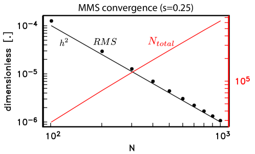
Figure 2: Convergence of MMS solution $u=\sin(2\pi x)+1$ for $s=0.25$ as a function of mesh size $N$ with corresponding node spacing $(N-1)^{-1}$. In symbols is the RMS residual; black lines, the curve $h^{2}$; and in red, the total number of degrees of freedom in the discretized linear system (27). Linear system (27) is solved using BiCG-STAB to a tolerance of $10^{-16}$ in RHS-normalized residual.

Figure 3: Convergence of BiCG-STAB algorithm with Jacobi preconditioning for the $N=101$ MMS solution in Figure 1. In the solid line is the average residual for equations in blocks $0,\ldots,L$ in (27) corresponding to fractional Helmholtz equations on $v_{\ell}$; dashed, the residual for equations in block $L+1$ corresponding to solution of the Laplace equation for $w$; and dotted, the residual for the final $(L+2)$ block of equations enforcing compatibility between $v$ and $v_{\ell}$.

Lastly, we confirm that the choice $m=1/\log{1\over h}$ for quadrature spacing (and by extension, the number $L$ of $v_{\ell}$ equations) is nearly optimal by examining the effect on RMS of varying $m$. As a representative example, the $N=101,s=0.25$ discretization of the MMS problem is solved for a range of $m$ values around $1/\log{1\over h}$. In this example the asymptotic limit for minimum RMS value is achieved at $m$ roughly 90% of its optimal value, where the asymptotic limit is driven by the error of the finite element discretization itself (Fig. 4). In contrast, choices of $m$ larger than the optimal value result in a rapidly increasing RMS, consistent with the exponential convergence of quadrature error reported elsewhere [10].

Figure 4: Convergence of RMS error as a function of quadrature spacing $m$ for the MMS problem with $N=101,h=0.01$ finite element nodes (see Fig. 2). Optimal quadrature interval $m^{*}$ is given by (11) yields $\text{RMS}=1.25\times 10^{-4}$, a value close to the asymptotic limit when $m<m^{*}$. Note the rapidly increasing RMS error as $m^{*}<m$.

5 Numerical Results

Our fractional Helmholtz system is numerically demonstrated in the context of magnetotellurics (MT). This is a geophysical surveying method that measures naturally occurring, time-varying magnetic and electric fields. Resistivity estimates of the subsurface can be derived, from the very near surface to hundreds of kilometers, that are applied to subsurface characterization for geoscience application, such as hydrocarbon extraction, geothermal energy harvesting, and carbon sequestration, as well as studies into Earth’s deep tectonic history. The MT signal is caused by the interaction of the solar wind with the earth’s magnetic field (lower frequencies less than 1 Hz) and world-wide thunderstorms, usually near the equator (higher frequencies greater than 1 Hz). Figure (5) provides a conceptual diagram of MT in which the ionosphere is the electromagnetic source (see Section 2) for inducing currents in the subsurface. Because the magnitude of this source current is unknown, the fundamental quantity for MT analysis is the impedance tensor mapping electric correlated electric and magentic fields. Computed in the frequency domain, the impedance tensor is an estimate of the Earth “filter” mapping magnetic to electric fields – in other words, it is an expression of Earth’s conductivity distribution. Common in preliminary MT analysis is the assumption of locally 1D (depth dependent) electrical structure and excitation by a vertically incident plane wave, such as described in Section 2. We adopt these modest assumptions in our investigation of MT data – in particular, data collected by the decadal, trans–continental USArray/Earthscope project [27] – and find examples where MT data is consistent predicted impedances for a fractionally–diffusing electromagnetic Earth.

Because of the novelty in applying fractional derivative concepts to electromagnetic geophysics, the first question that draws our attention is simply: How does a fractionally diffusing field, as described by (3) and (4), compare to a field derived from the classical Helmholtz equation? To address this question we solve (4) on the dimensionless unit interval $\zeta\in[0,1]$ with unit amplitude Dirichlet conditions $u(0)=\sqrt{2\text{i}}$ and $u(1)=0$ on the horizontal electric field and choose the dimensioned scaling factor $z^{*}=1000$ m to represent the physical domain $z\in[0,1000]$ m. Choice of homogeneous Dirichlet condition at $\zeta=1$ is commonly known as “perfectly conducting” boundary condition, representing the presence of an infinitely conductive region for $\zeta>1$, but is used here strictly out of computational convenience. Scattering from this interface back to Earth’s surface $\zeta=0$ will be negligible as long as the frequency $\omega$ in Equation (4) is sufficiently high that the electric field at depth is essentially zero. The unit interval is discretized with 501 evenly distributed nodes, on which the electric field is drawn from the finite dimensional vector space of linear nodal finite elements. Hence, node spacing is $h=0.002$, which, when $s=0.7$ for example, leads to $N^{-}=318$ and $N^{+}=137$ according to (11) and a linear system (27) with $501(3+N^{-}+N^{+})=229458$ equations. Comparable to the error tolerances on the BiCG-STAB solver specified previously for the MMS problem, the iterative sequence is terminated once the normalized residual is reduced by $10^{-12}$ over its starting value.

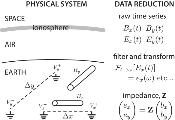
Figure 5: Overview of magnetotelluric experiment and data reduction. (left) Collocated time series of horizontal electric field, measured by pairs of grounded electrodes, and magnetic field, measured by induction coils or fluxgates, measure Earth’s inductive response to ionspheric source currents. (right) Time series are windowed, filtered and transformed into the frequency domain, from which the impedance tensor is estimated, containing information on the distribution of electricical conductivity variations in Earth’s subsurface [13]. Because high–frequency fields decay more rapidly with depth than low frequency fields, frequency can loosely be interpreted as a proxy for depth, and hence an impedance spectrum is a coarse measure of the local, depth variations in electrical conductivity.

The horizontal electric fields in Fig. 6 show depth–dependent behavior that is clearly also $s$-dependent: increased curvature in the near–surface and decreased curvature at depth in comparison with their classical $s=1.0$ counterpart. This suggests that the effect of the fractional Laplacian in (3) and (4) over a uniform $\sigma_{\alpha,\zeta}$ Earth model is, at first blush, in some ways similar to that of a classical Laplacian over a layered Earth which is conductive in the near surface and resistive at depth. However, closer inspection of the fractional response (see, for example the $s=0.60$ curves) reveals that the damped oscillations, characteristic of classical Helmholtz, are simply not present as $s$ decreases from unity, and instead then are replaced with a steady non–oscillatory decay with depth.

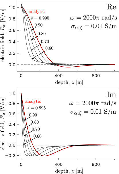
Figure 6: For a range of fractional exponent values $s=0.6,0.7,0.8,0.9,0.995$, decay of unit–amplitude real (top) imaginary (bottom) components of horizontal electric field $E_{x}=u$ as a function of depth $z$ into a uniform $\sigma_{\alpha,\zeta}=0.01$ S/m medium at frequency $f=1$ kHz, corresponding to dimensionless wavenumber $\kappa\approx 8.89$. In red is the analytic solution for the corresponding classical $s=1$ Helmholtz. See text for additional details on boundary conditions and scaling to the physical domain from the dimensionless unit interval.

There is a dramatic manifestation of this fractional Helmholtz response in observable magnetotelluric data through calculation of the impedance spectrum (Fig. 7). Amplitude of the impedance spectrum, reported here as the familiar apparent resistivity

$$\rho_{a}={1\over\omega\mu_{0}}\Big{|}{E_{x}\over H_{y}}\Big{|}^{2}_{z=0}=\omega\mu_{0}(z^{*})^{2}\Big{|}{u\over\partial_{\zeta}u}\Big{|}^{2}_{\zeta=0}$$ (30)

and complex phase angle $\theta$ of the ratio $-u/\partial_{\zeta}u$, show a clear $s$–dependence at frequencies above 1 Hz. Decay of the apparent resistivity as frequency approaches zero can be understood as a consequence of the perfect electric conductor boundary condition at $z=z*$, where at these low frequencies the reciprocal wavenumber ${1\over\kappa}>>z^{*}$ and hence the apparent resistivity approaches that of the perfect conductor, zero, in the region $z>z^{*}$. Furthermore, in the limit of zero frequency, the fractional Helmholtz equation asymptotes to the fractional Laplacian equation (analagous to (8)) with inhomogeneous Dirichlet boundary conditions, whose solution has already been established [3] as equivalent to the classical Laplacian equation, leaving the ratio ${-u/\partial_{\zeta}u}=1$, or equivalently $\theta=0$.

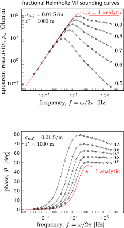
Figure 7: Magnetotelluric sounding curves for a uniform $\sigma_{\alpha,\zeta}$ Earth model over the depth domain $z\in[0,z^{*}]$ for a range of fractional exponent values $s=0.5,\ldots,1.0$ with a perfect conductor boundary condition at $z=z^{*}$. Apparent resistivity (top); complex phase (bottom). See text for description. In red are the classical $s=1$ Helmholtz solutions, computed analytically.

The decrease in apparent resistivity at high frequencies when $s\neq 1$ can further be understood by examination of the electric field gradient at $z=0$ (Fig. 8). Although there is a slight decrease in the vertical gradient of the imaginary component of electric field when $s\neq 1$, the magnitude of the real component increases dramatically in comparison to the $s=1$ case. This overall rise in vertical gradient at the air/earth interface for a fractional Earth model decreases the value of the quotient in (30), thereby leading to a decreased estimate of the apparent resistivity at large frequencies.

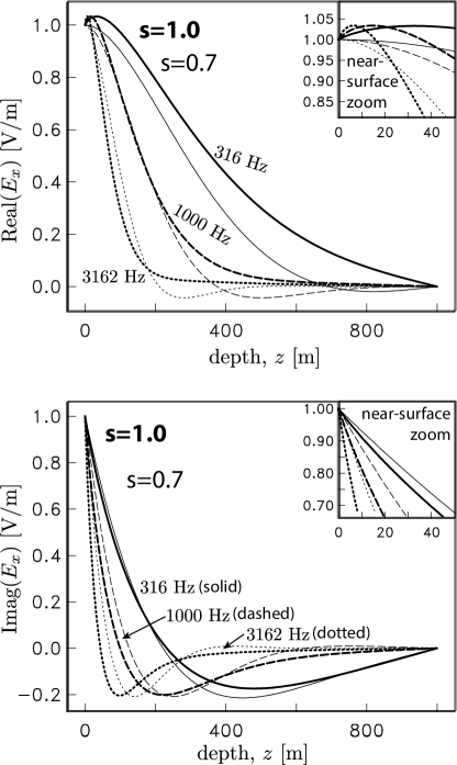
Figure 8: Real (top) and imaginary (bottom) components of horizontal electric field as a function of depth in a uniform 0.01 S/m Earth underlain by a perfect conductor for frequencies $f=316,1000$ and 3162 Hz, corresponding to the high–frequency region of the magnetotelluric apparent resistivity spectrum (Fig. 7) with approximate $s$ dependent power law behavior. Curves for classical $s=1$ (heavy lines) and fractional $s=0.7$ response (light lines) are shown. The decrease in apparent resistivity is evidently due to the strongly increased vertical gradient of Real component of electric field at the air/Earth interface $z=0$ for fractional Helmholtz. Recall that from Eq (4.1) that the vertical gradient of electric fields resides in the denominator of the of the apparent resistivity estimator.

5.1 Validation through USArray data

We have made progress towards validating our hypothesis of “fractional Helmholtz leading to new geophysical interpretation” though geophysical insight of numerical experiments. Results suggests complex material properties in the subsurface exposed to electromagnetics energy exhibit conductive behavior near surface, resisistive at depth. Additional evidence of superdiffusice behavior can be observed from MT data at the USArray station NW Kansas City. Apparent resistivity and phase angle data from USArray MT station for KSP34 located NW of Kansas City, KS, USA show show similar non-local behavior as our numerical experiments. Figure (9) shows apparent resistivity and phase angle versus frequency, as well as resistivity versus depth, which exhibit non-local characteristics in the subsurface geology. An in-depth study of the geology in the Kansas City region would futher endorse our observations but is beyond the scope of this paper. These field data correlations however provide further motivation to support additional algorithmic development for fractional electromagnetics.

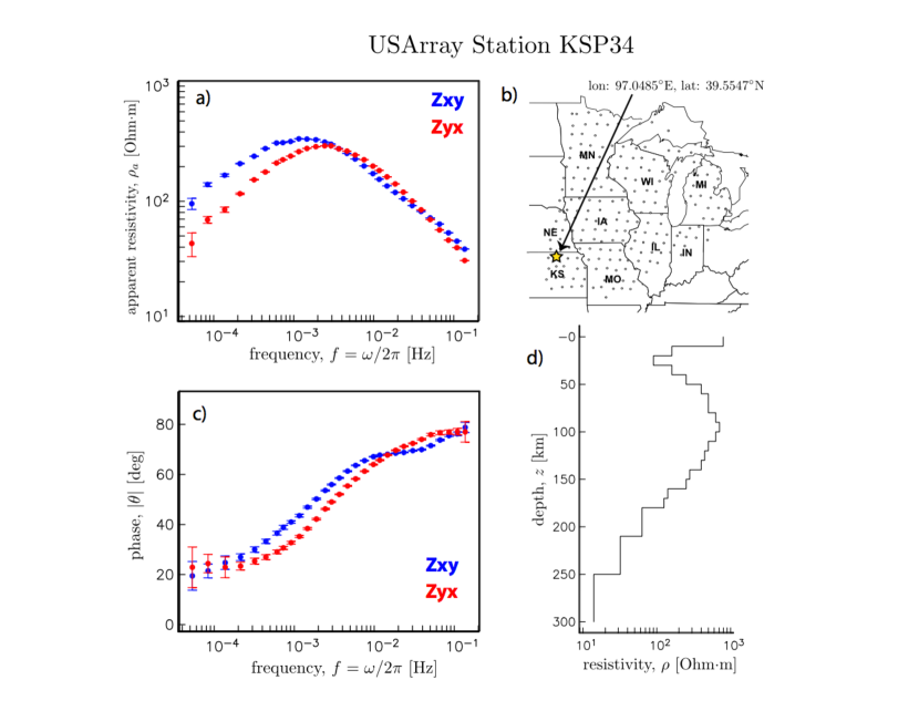
Figure 9: Apparent resistivity and phase angle data from USArray MT station for KSP34 located NW of Kansas City, KS, USA from the US Array: a) Apparent resisistivity spectrum based on Zxy (blue) and Zyx (red) elements of the $2\times 2$ impedance tensor $\mathbb{Z}$. The similarity in the curves, especially at high frequencies, is indicative a locally 1D conductivity profile beneath the observation point. b) Location map for USArray MT station KSP34. c) Complex phase angle of the ratios $E_{x}$/$H_{y}$ (Zxy, blue) and $E_{y}$/$H_{x}$ ($Z_{yx}$, red), again generally similar and indicating a locally 1D conductivity profile beneath the station. d) Depth profile of electrical resistivity beneath station KSP34 estimated by 3D inversion of all sites in sub-panel (b) (figure 3, sub-panel (a), Yang et al., EPSL 2015 ).

5.2 Strategies for a spatially–variable fractional exponent

An initial assumption in problem statement (5) is the spatial invariance of the fractional exponent $s$ over the spatial domain $\Omega$. However, if $s$ is intepreted to represent via non–locality some degree of long–range correlation of underlying material properties (e.g. electrical conductivity), then it is relevant to consider how spatial variability in this correlation is accommodated in the architecture of the fractional calculus paradigm. In addition, variability in $s$ enables us to truly capture the non-smooth effects such as fractures by prescribing variable degree of smoothness across the scales. A detailed analysis for variable $s$, where the authors have created a time-cylinder based approach, has been recently carried out in [6]. For a precise definition of the fractional Laplacian with variable $s$ we refer to [1].

In the case of a piecewise constant $s$, a conceptually simple strategy is to decompose the domain $\Omega$ into subdomains on which $s$ is constant and impose our Kato method over each of the subdomains. Note that the solution for $w$ in (8) is independent of $s$ and may be obtained without any need for domain decomposition. Although differences in $s$ among domains means that the number of functions $v_{\ell=0,\ldots,L}$ also varies among domains, the boundary condition $v=0$ on each of the subdomains ensures continuity of $v$, and therefore continuity of $u=v+w$ throughout $\Omega$. Observe that computation of $\{v_{\ell}\}$ in one subdomain is independent of its calculation in another, and hence, $\{v_{\ell}\}$ over each of the subdomains can computed in parallel with no message passing or interdomain communication required once $w$ is solved for and shared globally throughout $\Omega$. That said, several issues need to be resolved before this idea can be defensibly implemented. First, the suggestion of zero (subdomain) boundary conditions on $\{v_{\ell}\}$ needs to be physically justified. If found to be unsound, the embarrassingly parallel structure just described will instead require interdomain communication and potentially interpolation. Second, because the fractional Laplacian is inherently non–local, its support extends over the global domain $\Omega$. Ensuring global extent of non–locality in the context of subdomains requires further analysis. Lastly, function and flux continuity for a given $v_{\ell}$ within a subdomain is guaranteed; the conditions for such guarantees, in a general sense, at subdomain boundaries have yet to be determined. Because of these complexities, further analysis of this domain decomposition concept is deferred to future publication.

5.3 Fractional time derivatives

Prior work in electromagnetic geophysics in contemplation of Ohm’s constitutive law being represented in terms of fractional calculus have focused on fractional time derivatives, rather than the fractional space derivatives described here [30, 16, 18]. Such analyses are comparatively simple in that the fractional space derivatives $D_{z}^{\alpha}$ of (1.2) are replaced by time derivatives $D_{t}^{\beta}$, thus modifying the complex wavenumber as $k^{2}=-(\text{i}\omega)^{1-\beta}\mu_{0}\sigma$. Solutions to (5) in layered media when $s=1$ (equivalently, $\alpha=0$ since $s=1-{\alpha\over 2}$) follow the usual method of posing characteristic solutions $\exp(\pm kz)$ in each of the layers, coefficients for which are determined through enforcement of boundary condition (5) along with continuity of $u$ and $\partial_{z}u$ at layer boundaries. Solving this time-fractional Helmholtz equation on the domain $\Omega:z\in[0,z^{*}=1000]$ m with $u(0)=1+\text{i}$, $u(z^{*})=0$ and $\sigma=0.01$ S/m$(\text{rad/s})^{-\beta}$ yields a characteristic magnetotelluric response (Fig. 10) distinct from that obtained in the case of space–fractional derivatives $s\neq 1$ (Fig. 7). As noted in [18], imposing the time–fractional derivative in this way is equivalent to recasting real–valued electrical conductivity $\sigma$ as a frequency–dependent, complex–valued conductivity $\sigma(\text{i}\omega)^{\beta}$. The quasi–linear power–law behavior in apparent resistivity and phase angle (Fig. 10) seen at high frequencies ($f>100$ Hz) is objectively distinct from that computed for the space–fractional Helmholtz system (Fig. 7) and offers an unambiguous diagnostic for discriminating between the two. These differences have their origin in the how anomalous power–law diffusion is captured by each. In the case of fractional time derivatives of order $1-\beta$, as considered in this latest example, the system is considered subdiffusive and consistent with an anomalously high likelihood of long wait times between successive jumps of charge carriers in a continuous time random walk as might be applied to fluid transport in a porous medium [23]. Instead, the space–fractional derivatives which occupy the primary focus of the present study capture long–range interactions (spatial nonlocality) of charge carriers as a superdiffusive system, perhaps through inductive coupling (a phenomena absent in the physics of fluid flow in porous media). This contrast – super- versus sub-diffusion – is the essence of the causative physics behind the different magnetotelluric responses predicted by (Fig. 7 and Fig. 10).

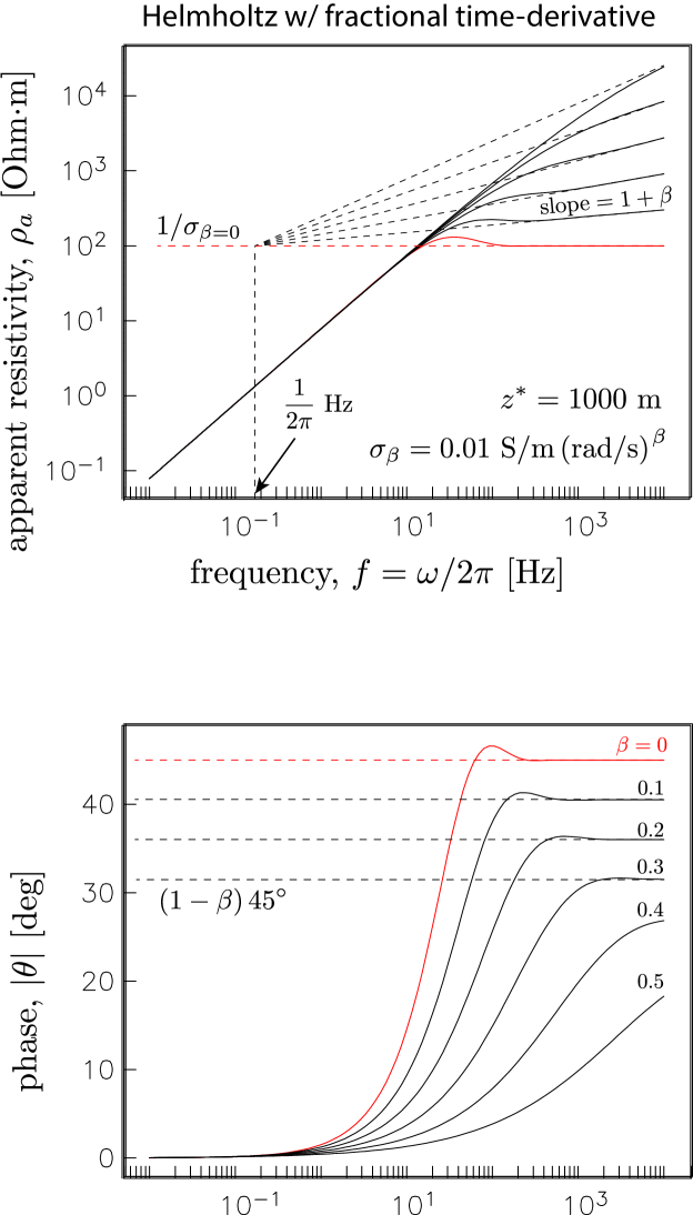
Figure 10: Apparent resistivity spectra for classical Helmholtz equation $s=1$ with $\text{i}\kappa^{2}=(\text{i}\omega)^{1-\beta}\mu_{0}\sigma$, where the $\beta$ terms arise in the 1D magnetotelluric case from Ohm’s law with a fractional, non–local time dependence attributable to sub-diffusion of electric charge following a continuous time random walk with a heavy–tailed distribution of waiting times. Compare to Fig. 7 for the space–fractional case describing super–diffusion, where the heavy–tailed distribution of step length (a.k.a. Lévy flights) captures long–range interactions between charges.

6 Conclusions

We have presented a novel, practical solution to the fractional Helmholtz equation based on the Kato formulation of the fractional Laplacian operator, a lifting (splitting) strategy to handle non-zero Dirichlet boundary conditions, and finite element discretization of the spatial domain. This specific finite element discretization derives from our statement of the variational problem, from which alternative discretizations (orthogonal polynomials, wavelets, spectral functions, etc.) offer an interesting direction for future research. Whereas the analogous Kato/lifting strategy for solving the fractional Poisson equation leads to decoupled system of integer Laplace solves which can be done in parallel with no inter-solve communication, solution of the fractional Helmoltz admits no such decoupling. This leads to a large, block–dense system of linear equations upon discretization which significantly increases the resource requirements for obtaining a numerical solution. In response, we augment the variational problem by introducing an additional unknown which collapses the $L-1$ block coupling matrices in a given block–row into a single block matrix, at the expense of only one additional (dense) block–row in the linear system. For typical problems where with $L>>100$, the added computational burden of this compatibility equation is inconsequential, yet the reduction in matrix storage is significant, going from $L^{2}$ to simply $2L$. Thus, a key feature of this augmented variational problem is the extreme block–sparsity of the resulting linear system of equations, a feature which is independent of the choice of discretization and important for efficient solution of large–scale systems. Validation of the algorithm for linear, nodal finite elements shows $h^{2}$ reduction in RMS error for an MMS test problem – demonstrating that our formulation of the fractional Helmholtz problem does not corrupt the convergence behavior expected from solution of integer-order Helmholtz.

We apply this formulation for fractional Helmholtz to the growing body of observational evidence of anomalous diffusion in nature – here, asking the question, “Does the Earth, with its incalculable geologic complexity, respond to electromagnetic stimulation in a way that is consistent with fractional diffusion and the non–locality that is central to the differential operators of the governing physics”? Whereas temporal non-locality of Maxwell’s equations has previously been observed as sub–diffusive propagation, the fractional Helmholtz equation studied here describes super–diffusion by attributing fractional derivatives directly to the spatial distribution of material properties in Ohm’s constitutive law. Earth electromagnetic response is computed in the context magnetotelluric (MT) analysis – a classic geophysical exploration technique dating back to to middle 20th century – and comparison with the EarthScope USArray database. We find qualitative agreement between the predicted fractional Helmholtz response functions and those observed at a middle North American measurement site. This congruence in electromagnetic response thereby offers an altenative interpretation of the MT data at the site, one where the classical interpretation of a layered Earth geology with deep resistive rocks overlain by a conductive overburden is contrasted with new interpretation suggesting complex, geologic texture consistent with the site’s proximity significant deep crustal tectonic structure.

Outstanding issues for future research therefore lie in two fundamental areas: arriving at a clearer mapping between the value of a fractional exponent $s$ and the material heterogeneity it’s intended to represent; and, extension of the computational tools to higher dimension with parallel implementation, including spatially variable and/or anisotropic $s$ values. The former may be informed, as we’ve done here, by reinterpretation of existing observational data through fractional calculus concepts, but augmented by detailed material analysis. The latter naturally feeds into ongoing efforts in PDE–constrained optimization for material property estimation, now augmented with the desire to recover $s$, too, as a measure of material complexity or sub–grid structure. Algorithmic advances in multi-level domain decomposition (decomposition over physical domain in addition to decomposition over the functional blocks of global system matrix) will also be required for full exploration of fractional Helmholtz concepts on large, 3D domains.

References

- [1] H Antil, A Ceretani, and C N Rautenberg. The fractional Laplacian with spatially variable order. 2018. (in prep).
- [2] H. Antil and J. Pfefferer. A short matlab implementation of fractional poisson equation with nonzero boundary conditions. Technical Report, 2017. http://math.gmu.edu/~hantil/Tech_Report/HAntil_JPfefferer_2017a.pdf, accessed Sept 13, 2018.
- [3] H. Antil, J. Pfefferer, and S. Rogovs. Fractional operators with inhomogeneous boundary conditions: Analysis, control, and discretization. Communications in Mathematical Sciences (CMS), 16(5):1395–1426, 2018.
- [4] H. Antil and M. Warma. Optimal control of fractional semilinear pdes. To appear: ESAIM: Control, Optimisation and Calculus of Variations (ESAIM: COCV), 2019.
- [5] Harbir Antil, Johannes Pfefferer, and Mahamadi Warma. A note on semilinear fractional elliptic equation: analysis and discretization. ESAIM. Mathematical Modelling and Numerical Analysis, 51(6):2049–67, 2017. doi:10.1051/m2an/2017023.
- [6] Harbir Antil and Carlos N Rautenberg. Sobolev spaces with non-muckenhoupt weights, fractional elliptic operators, and applications. arXiv:1803.10350, 2018. https://arxiv.org/pdf/1803.10350.pdf, accessed Sept 27, 2018.
- [7] D. A. Benson, S. W. Wheatcraft, and M. M. Meerschaert. The fractional-order governing equations of lévy motion. Water Resources Research, 36(6):1413–1423, June 2000.
- [8] M Berggren. Approximations of very weak solutions to boundary–value problems. SIAM Journal of Numerical Analysis, 42:860–77, 2004.
- [9] A Bonito and JE Pasciak. Numerical approximation of the fractional powers of regularly accretive operators. IMA Journal of Numerical Analysis, 37:1245–73, 2017.
- [10] Andrea Bonito and Joseph E. Pasciak. Numerical approximation of fractional powers of elliptic operators. Mathematics of Computation, 84(295):2083–2110, 2015. doi:10.1090/S0025-5718-2015-02937-8.
- [11] Luis A. Caffarelli and Pablo Raúl Stinga. Fractional elliptic equations, Caccioppoli estimates and regularity. Annales de l’Institut Henri Poincaré. Analyse Non Linéaire, 33(3):767–807, 2016. doi10.1016/j.anihpc.2015.01.004.
- [12] M Caputo. Models of fluids in porous media with memory. Water Resources Research, 36(3):693–705, 2000.
- [13] A D Chave and A G Jones. The Magnetotelluric Method: Theory and Practice. Cambridge University Press, Cambridge, UK, 2012.
- [14] L Deseri and M Zingales. A mechanical picutre of frational-order darcy equation. Communications in Nonlinear Science and Numerical Simulation, 20:940–949, 2015.
- [15] J Elser, V A Podolskiy, I Salakhutdinov, and I Avrutsky. Nonlocal effects in effective–medium response of nanolayered metamaterials. Applied Physics Letters, 90:191109, 2007. doi:10.1063/1.2737935.
- [16] M E Everett. Transient electromagnetic response of a loop source over a rough geologic medium. Geophysical Journal International, 177:421–429, 2009. doi:10.1111/j.1365-246X.2008.04011.x.
- [17] Mark E. Everett and Chester J. Weiss. Geological noise in near-surface electromagnetic induction data. Geophysical Research Letters, 29(1):1010, 2002. doi:10.1029/2001GL014049.
- [18] J Ge, M E Everett, and C J Weiss. Fractional diffusion analysis of the electromagnetic field in fractured media – Part 2: 3D approach. Geophysics, 80:E175–E185, 2015. doi:10.1190/geo2014-0333.1.
- [19] S-I Karato and D Wang. Electrical conductivity in rocks and minerals. In S-I Karato, editor, Physics and Chemistry of the Deep Earth, chapter 5, pages 145–184. John Wiley & Sons, Ltd., Chichester, UK, 2013. doi:10.1002/9781118529492.ch5.
- [20] Tosio Kato. Note on fractional powers of linear operators. Proceedings of the Japan Academy, 36(3), 1960.
- [21] J L Lions and E Magenes. Non–homogeneous Boundary Value Problems and Applications. Springer–Verlag, Berlin, 1972.
- [22] Mark M Meerschaert and Anna Sikorskii. Stochastic Models for Fractional Calculus. Walter de Gruyter GmbH & Co. KG, Berlin/Boston, 2012.
- [23] R Metzler and J Klafter. The random walk’s guide to anomalous diffusion: a fractional dynamics approach. Physics Reports, 339:1–77, 2000. doi:10.1016/S0370-1573(00)00070-3.
- [24] P J Roache. Verification of codes and calculations. American Institute of Aeronautics and Astronautics Journal, 36:696–702, 1998.
- [25] Kambiz Salar and Patrick Knupp. Code verification by the method of manufactured solutions. Technical report, Sandia National Laboratories, 2000. SAND2000-1444.
- [26] R Song and Z Vondraček. On the relationship between subordinate killed and killed subordinate processes. Electronic Communications in Probability, 13:325–36, 2008.
- [27] USArray. Earthscope usarray magnetotelluric (mt) program. http://www.usarray.org/researchers/obs/magnetotelluric.
- [28] H A van der Vorst. BI-CGSTAB: A fast and smoothly converging variant of BI-CG for the solution of nonsymmetric linear systems. SIAM Journal of Scientific and Statistical Computing, 13:631–644, 1992.
- [29] A. von Kameke, F. Huhn, G. Fenandez-Garcia, A.P. Munuzuri, and V. Perez-Munuzuri. Propagation of a chemical wave front in a quad-two-dimensional superdiffusive flow. Physical Review E, 81(066211), 2010.
- [30] C J Weiss and M E Everett. Anomalous diffusion of electromagnetic eddy currents in geologic formations. Journal of Geophysical Research, 112:2006JB004475, 2007.