WavePacket: A Matlab package for numerical quantum dynamics.
III: Quantum-classical simulations and surface hopping trajectories

Abstract

WavePacket is an open-source program package for numerical simulations in quantum dynamics. It can solve time-independent or time-dependent linear Schrödinger and Liouville-von Neumann-equations in one or more dimensions. Also coupled equations can be treated, which allows, e.g., to simulate molecular quantum dynamics beyond the Born-Oppenheimer approximation. Optionally accounting for the interaction with external electric fields within the semi-classical dipole approximation, WavePacket can be used to simulate experiments involving tailored light pulses in photo-induced physics or chemistry. Being highly versatile and offering visualization of quantum dynamics ’on the fly’, WavePacket is well suited for teaching or research projects in atomic, molecular and optical physics as well as in physical or theoretical chemistry.

Building on the previous Part I [Comp. Phys. Comm. 213, 223-234 (2017)] and Part II [Comp. Phys. Comm. 228, 229-244 (2018)] which dealt with quantum dynamics of closed and open systems, respectively, the present Part III adds fully classical and mixed quantum-classical propagations to WavePacket. In those simulations classical phase-space densities are sampled by trajectories which follow (diabatic or adiabatic) potential energy surfaces. In the vicinity of (genuine or avoided) intersections of those surfaces trajectories may switch between surfaces. To model these transitions, two classes of stochastic algorithms have been implemented: (1) J. C. Tully’s fewest switches surface hopping and (2) Landau-Zener based single switch surface hopping. The latter one offers the advantage of being based on adiabatic energy gaps only, thus not requiring non-adiabatic coupling information any more.

The present work describes the MATLAB version of WavePacket 6.0.2 which is essentially an object-oriented rewrite of previous versions, allowing to perform fully classical, quantum–classical and quantum-mechanical simulations on an equal footing, i. e., for the same physical system described by the same WavePacket input. The software package is hosted and further developed at the Sourceforge platform, where also extensive Wiki-documentation as well as numerous worked-out demonstration examples with animated graphics are available.

I Introduction

Progress in the generation of short intense laser pulses and related experimental techniques on an ultra-fast time scale has lead to substantial advances in atomic and molecular physics and related fields in the late 20th century Zewail (2000). This has also motivated new developments in theoretical and simulation studies of quantum molecular dynamics in recent years May and Kühn (2000); Tannor (2004). However, despite the obvious need, general-purpose and freely available simulation software in this field is still scarce. Among the exceptions, there is the versatile MCTDH package which has evolved into a quasi-standard in quantum molecular dynamics Beck et al. (2000). In addition, there is also the TDDVR package in that field Khan et al. (2014). Software packages more commonly used in the physics community include QuTiP for the dynamics of open quantum systems Johansson et al. (2013), the FermiFab toolbox for many-particle quantum systems Mendl (2011), and the QLib platform for numerical optimal control Machnes et al. (2011). The present article deals with the WavePacket software package. Its main version which is coded in Matlab has been described in a series of two recent articles Schmidt and Lorenz (2017); Schmidt and Hartmann (2018). Part I focuses on closed quantum systems and the solution of Schrödinger equations, with emphasis on discrete variable representations (DVR), finite basis representations (FBR), and various techniques for temporal discretization Schmidt and Lorenz (2017). Part II is mainly on open quantum systems and the solution of Liouville–von Neumann equations, optimal control of quantum systems and their dimension reduction Schmidt and Hartmann (2018). It is emphasized that the target systems for WavePacket are low- to medium-dimensional (model) systems where computational requirements are not the dominant concern. Instead, the user-friendliness of the Matlab environment and, in particular, the ability of generating on-the-fly graphics have attracted an increasing number of users. As such, WavePacket is very suitable not only for educational purposes, but also for development, implementation and testing of various numerical techniques and algorithms which is facilitated by the highly modular structure of the software package.

While fully quantum-dynamical simulations are nowadays routinely carried out for small molecules, the treatment of larger systems such as atomic and molecular clusters, biologically relevant molecules, and condensed matter systems remains a challenge due to the high computational effort. Despite impressive progress in numerical quantum dynamics, especially by the multi-layer extensions of the MCTDH Wang and Thoss (2003) methodology, there is still the need for more approximate classical or mixed (hybrid) quantum-classical computational methods. Those represent an important alternative not only because their computational effort scales more favorably with the system size, but often also because they provide intuitive insight into the dynamics of molecular processes. Among these approaches is the surface hopping trajectory (SHT) simulation technique. The basic idea of SHT is to propagate classical trajectories for the heavy particles (typically nuclei) which may statistically hop between different quantum states of the light particles (typically electrons) subsystem thus modeling nonadiabatic transitions in a simple way. Even though the seminal paper by J. C. Tully on the fewest switches surface hopping (FSSH) algorithm was published almost 30 years ago Tully (1990) this method is still in active use, due to its low computational expense and its extremely simple implementation. In the chemical community, this technique has become routinely available through its implementation in software packages such as Newton-X Barbatti et al. (2014), Fish Mitrić et al. (2009), Sharc Richter et al. (2011); Mai et al. (2018) providing a combination of SHT techniques with standard electronic structure software packages. In those approaches, the forces and the nonadiabatic couplings governing the trajectories are computed “on-the-fly” by means of ab initio or semi-empirical electronic-structure calculations.

Moreover, there has been substantial methodological progress in SHT simulations in recent years Tully (2012); Wang et al. (2016). On the one hand, these efforts aim at overcoming the known problems of the earlier SHT approaches. Among others, the lack of communication between the evolving trajectories leads to overcoherence, and limitations in the energy conservation are hampering a description of superexchange processes Subotnik et al. (2016); Wang et al. (2016). On the other hand, also the SHT algorithm itself has been improved. In the so-called single switch surface hopping (SSSH) approach there is only a single switch decision required each time a trajectory passes a critical region, typically a (genuine or avoided) crossing seam or conical intersection. The transition probabilities in these SSSH algorithms are calculated from Landau-Zener (LZ) formulae Lasser et al. (2007); Lasser and Swart (2008); Fermanian Kammerer and Lasser (2008). Of particular interest is a variant which is entirely based on adiabatic energy gaps, thus rendering the need for nonadiabatic coupling information completely redundant Belyaev and Lebedev (2011); Belyaev et al. (2014, 2015).

In this work, we present the implementation of classical trajectory and SHT propagation techniques (both FSSH and SSSH variants) into the most recent Matlab version of WavePacket 6.0.2. This has been made possible through an object-oriented rewrite of previous versions of WavePacket which were described in Part I Schmidt and Lorenz (2017) and Part II Schmidt and Hartmann (2018). The main goal of using such a programming technique is to perform fully classical, mixed quantum-classical and fully quantum-mechanical simulations on an equal footing. This allows for a direct comparison of the respective evolutions for the same physical system, i. e., for the same Hamiltonian, initial conditions, time stepping etc. which can be defined in the same WavePacket input file. Such a comparison strongly benefits from the generation of graphical output which has always been one of the key advantages of the Matlab version of WavePacket. Quantum and (quantum-)classical propagations are visualized in the same way, with a large variety of different options such as curve plots, contour plots, surface plots, etc. available, which helps the user to develop a more intuitive understanding of the respective type of dynamics.

In addition to the mature Matlab version of WavePacket presented here, there is also a C++ version which is however still in a very early stage of development. Both versions are hosted and further developed at the open source SourceForge platform where also extensive Wiki documentation as well as a large number of demonstration examples can be found.

II WavePacket workflow

A typical workflow for a dynamical WavePacket simulation could be as follows

qm_setup();
state=wave(); | state=traj();
qm_init(state);
qm_propa(state);
qm_cleanup();

After calling the function qm_setup which opens the logfile and purges the workspace from previous calculations, the second command creates an object named state. This object can be an instance of either one of the following two classes: Class wave is meant for fully quantum-mechanical simulations dealing with wavefunctions represented on grids. In contrast, class traj is designed for fully classical or hybrid quantum-classical simulations, based on classical densities sampled by swarms of trajectories. Note that such objects were not yet in use in version 5 described in Part I and Part II. Once being constructed, these objects may be modified within the initialization function qm_init which is intended to set many parameters defining the physical system and which has to be provided by the user separately for every simulation; for more information, see Sec. III. Next, the object state is propagated in time by calling the function qm_propa which represents the main workhorse of the WavePacket software package. For in-depth explanation of quantum-mechanical or quantum-classical propagations, see Sec. IV or Sec. V, respectively. Finally, the function qm_cleanup closes the logfile and does other minor cleanup. Note that in the Matlab script given above the function qm_propa could be replaced by qm_bound which performs a bound state calculation instead of a propagation, see Sec. 5 of Part I, which is available for objects of type wave only. Another alternative would be to replace the function qm_propa by qm_movie in which case no propagation is carried out but animated graphics is created from previously generated simulation data, see Sec. 6 of Part I.

In general, constructor methods in Matlab can accept input arguments, typically used to assign the data stored in properties and return initialized objects. While in the second line of the sample script above, the constructors are called without passing any arguments, additional arguments may be passed when creating an instance of class traj. In the following example

state = traj (10000, 42);

an object encompassing 10000 trajectories is created. When the first parameter is not specified, a default value (1000 trajectories) will be assumed. The second parameter is used to seed the process of generation of pseudo-random numbers to ensure a predictable sequence of random numbers which may be useful for testing purposes. Note that if the seed is not set, a different sequence will be used in every propagation.

After a propagation with qm_propa has been carried out, calculated data is still available until the next purge by qm_setup. For example, the global variables time and expect holding the time stepping information and all expectation values, respectively, can be imported into the current workspace with the Matlab declaration global time expect. This information can be used, e. g., to display the populations as a function of the time given for the discretization points of the main temporal grid, see Sec. III.

In summary, the rationale behind the object-oriented rewrite leading to version 6 of the WavePacket software package is that it is now easily possible to compare fully quantum versus quantum-classical versus fully classical dynamics for exactly the same physical system (kinetic and potential energy, initial conditions, time stepping, etc.), specified by the same initialization file qm_init.m. Obviously, this goal is reached by polymorphism in the class definitions of wave and traj: In addition to containing all necessary data for the wave functions or trajectory bundles, repectively, these classes have to contain methods for setting up the initial conditions, the system’s Hamiltonian, and its application to the system’s state. Other implemented methods deal with the propagation itself as well as with the extraction of expectation values of observables.

Finally, it is mentioned that all the class definitions used throughout WavePacket 6 are realized as handle classes. In Matlab handle class constructors return handle objects, i. e., references to the object created. When passing such objects to functions, Matlab does not have to make copies of the original objects, and functions that modify handle objects passed as input arguments do not have to return them.

III Initialization of WavePacket

A closed, non-relativistic quantum mechanical system is characterized by a Hamiltonian operator

$$\hat{H}(R,-i\nabla_{R},t)=\hat{T}(R,-i\nabla_{R},t)+\hat{V}(R)$$ (1)

where $R$ is a position vector, $-i\nabla_{R}$ the corresponding momentum operator, and $T$ and $V$ are the kinetic and potential energy. Throughout the WavePacket software package, atomic units are used, i. e., Planck’s constant $\hbar$, the electronic mass and the elementary charge are scaled to unity. Semi-classical extensions of the Hamiltonian to include the coupling to external fields shall not be treated here; for more information on this the reader is referred to Parts I and II. The same holds for the use of negative imaginary potentials used to absorb densities near the edges of the domain.

Within the context of the present work it is of crucial importance that WavePacket can be employed not only for a single ($\nu=1$) but also for several ($\nu>1$) coupled Schrödinger equations in which case the Hamiltonian becomes a $\nu\times\nu$ operator matrix. The latter case arises naturally within the field of molecular quantum dynamics, where typically $R$ specifies the nuclear degrees of freedom and where $\nu$ is the number of electronic states involved in a close coupling calculation. Throughout this work, we will consider a prototypical example system with two spatial dimensions and with $\nu=3$ coupled channels. The diabatic representation of its Hamiltonian is given by

$${\mathbf{H}}^{\mathrm{(dia)}} = -\frac{1}{2M}\left(\frac{\partial^{2}}{\partial R_{1}^{2}}+\frac{\partial^{2}}{\partial R_{2}^{2}}\right)\mathbf{1}_{3\times 3}$$ (5)

$$+ \frac{1}{2}K\left(\begin{array}[]{ccc}(R_{1}+1/6)^{2}+R_{2}^{2}&0&0\\ 0&(R_{1}-1/6)^{2}+R_{2}^{2}&0\\ 0&0&(R_{1}-1/2)^{2}+R_{2}^{2}\end{array}\right)$$

$$+ \kappa\left(\begin{array}[]{ccc}0&R_{2}&0\\ R_{2}&0&R_{2}\\ 0&R_{2}&0\end{array}\right)$$ (9)

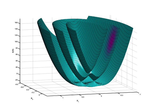
Figure 1: Adiabatic potential energy surfaces obtained from the Hamiltonian of Eq. (9) displaying three conical intersections. The blue-purple shading on the second surface indicates the initial density. Generated with WavePacket option: plots.density = vis.surface

with mass $M=100$, force constant $K=600$, and coupling constant $\kappa=100$. This Hamiltonian represents a generalization of the two–state Jahn-Teller Hamiltonian of Ref. Belyaev et al. (2014) to $\nu=3$, here with a value of $\epsilon=0.01$ for the quantum-classical smallness parameter which is typical for molecular systems. The eigenvalues of the (real symmetric) potential energy matrix yield the corresponding adiabatic potential energy surfaces displaying conical intersections at $R=(0,0)$, $R=(1/6,0)$, and $R=(1/3,0)$, see also Fig. 1.

All specifications of the above Hamiltonian, as well as further WavePacket settings explained below, have to be made by the user. This can be achieved with a user-defined function, which we suggest to call qm_init. Typically, this function begins as follows

function qm_init (state)
global hamilt plots space time

The second line serves to declare the most important variables inside WavePacket globally accessible. Note that it is a general policy throughout the Matlab version of WavePacket to use few, but highly structured variables to simplify book-keeping of variable names.

Subsequently, the spatial discretization has to be specified. Such grids are an essential ingredient of quantum-mechanical propagations of wavefunctions using objects of class wave, see Sec. III C of Part I. However, they also have to be specified for purely classical or quantum-classical propagations of trajectories using objects of class traj where they are used for graphical histogram representations of trajectory data. This guarantees similar appearance of graphical output, thus facilitating direct comparisons of quantum versus classical or quantum-classical dynamics. For the example of Eq. (9), the “tuning coordinate” $R_{1}$ is specified by an object of class fft (stored in folder +grid)

space.dof{1}       = grid.fft;
space.dof{1}.mass  = 100;
space.dof{1}.n_pts = 192;
space.dof{1}.x_min = -7/6;
space.dof{1}.x_max = +3/2;

Similarly, the spatial discretization of the “coupling coordinate” $R_{2}$ is also given by an object of class fft

space.dof{2}       = grid.fft;
space.dof{2}.mass  = 100;
space.dof{2}.n_pts = 192;
space.dof{2}.x_min = -2/3;
space.dof{2}.x_max = +2/3;

Here both coordinates are discretized using equally spaced grids allowing the use of FFT–methods when evaluating the kinetic operator. The number of points as well as the lower and upper boundaries are specified by the class properties n_pts, x_min, and x_max, respectively. Other discrete variable representations (DVRs), along with corresponding finite basis representations (FBRs) currently available in WavePacket are the Gauss–Legendre and Gauss-Hermite schemes, see Part I, which, however, are not yet available for classical propagations. Note that the implementation of space.dof as a Matlab cell vector provides some flexibility. In multidimensional simulations, such a vector can comprise objects of different classes thus allowing the use of different DVR schemes for different spatial degrees of freedom. In those cases, WavePacket represents wavefunctions and operators using direct products of the respective one-dimensional grid representations.

For propagations using qm_propa, also a temporal discretization has to be provided. For the example considered here, this can be achieved by setting the following properties of object time.steps

time.steps.m_start  = 000;
time.steps.m_stop   = 100;
time.steps.m_delta  = 0.025;
time.steps.s_number = 500;

which specifies 100 time steps with a constant width of 0.025. After each of these main time steps, expectation values of relevant observables are calculated and output to the Matlab console and the logfile. Internally, the main time steps are divided into shorter “substeps”, here 500 each, which are actually used as propagation steps for the short time propagators to be introduced in Secs. IV and V.

The variable time also contains information about the initial state. In the current example, the initial wave function is chosen to be a direct (outer) product of two Gaussian bell function which is realized by an object of class gauss (in the folder +init). The parameters for the Gaussian along $R_{1}$ are specified by

time.dof{1}       = init.gauss;
time.dof{1}.width = sqrt(0.005);
time.dof{1}.pos_0 = -1/2;
time.dof{1}.mom_0 = 0;

where the three properties serve to specify the width parameter as well as the center of the Gaussian in position and momentum representation. The parameters for the Gaussian along $R_{2}$ specified in time.dof{2} are the same as for $R_{1}$, except for the position which is $-1/20$. Note that in fully classical or quantum-classical propagations, initial values for the positions and momenta are obtained by drawing normally distributed random numbers from the corresponding Wigner transform of the initial wavefunction.

Next, the diabatic representation of the potential energy of Eq. (9) is defined by the following code lines

hamilt.coupling.n_eqs      = 3;
for m = 1:hamilt.coupling.n_eqs
    hamilt.pot{m,m}       = pot.taylor;
    hamilt.pot{m,m}.hshift = [(2*m-3)/6 0];
    hamilt.pot{m,m}.coeffs = [0 0; 600 600];
    for n = m+1:3
        if n==m+1
            hamilt.pot{m,n}        = pot.taylor;
            hamilt.pot{m,n}.coeffs = [0 100];
        else
            hamilt.pot{m,n}        = pot.taylor;
            hamilt.pot{m,n}.coeffs = [0 0];
        end
    end
end

where the first line specifies the number of coupled Schrödinger equations. The class taylor (stored in folder +pot) stands for a representation of the potential energy as a Taylor expansion the coefficients of which are given by class property coeffs. If required, the point of reference can be shifted horizontally or vertically, as specified by properties hshift and vshift, respectively.

It is emphasized that hamilt.pot is a Matlab cell matrix, thus permitting to define objects of different classes for the matrix entries which allows for high flexibility and easy customization. This includes the possibility of leaving certain matrix entries empty, e. g., when certain couplings are symmetry forbidden. In addition to the Taylor series representation, WavePacket comes with a rather large choice of class definitions for frequently used model potential functions, including spline interpolation to tabulated data. Of course, also user-supplied classes can be employed.

One of the hallmarks of the WavePacket software package is its ability to create graphical output ‘on the fly’, i.e., one movie frame is created for each main time step during a propagation using qm_propa. Thus, errors may be discovered already while the simulation is still running. To create visualizations of (classical or quantum densities) by, e. g. contour plots, an object of class contour (in the folder +vis) is created as follows

plots.density           = vis.contour;
plots.density.represent = ’dvr’;

where the second command is used to specify a representation in DVR (position space), as opposed to FBR (momentum space). Many other properties of the contour plots can also be specified, see the Wiki documentation at SF.net. Also note that the animation is saved as an MP4 file by default.

Besides contour plots, there are several other options to visualize densities in WavePacket such as curve plots, surface plots, flux plots, etc. For densities in higher dimensions, mainly from fully classical or hybrid quantum-classical simulations, there is also the possibility to calculate and display reduced densities in each of the dimensions or in pairs thereof. Additionally, curve plots of all relevant expectation values versus time are created by this command

plots.expect = vis.expect;

It is also possible to suppress graphical output by not creating objects named plots.density or plots.expect at all which may speed up WavePacket propagations considerably. In that context, it is noted that graphical output can be also created in retrospect. The WavePacket function qm_movie can be used to visualize (wavefunction or trajectory) data from previous runs of qm_propa provided that the following setting had been made

state.sav_export = true;

Further properties sav_dir and sav_file serve to specify directory and file name template, respectively, for saving the data.

IV Quantum-mechanical simulations

When providing an object of class wave as input argument, the WavePacket function qm_propa numerically solves the time-dependent Schrödinger equation (TDSE). Internally, this is always done using a diabatic representation $\mathbf{V}$ of the light particle (typically electrons) energies

$$\mathbf{H}^{\mathrm{dia}}=\mathbf{V}(R)-\frac{1}{2M}\Delta_{R}\mathbf{1}$$ (10)

For reasons of simplicity we have assumed only a single type of heavy particles (typically nuclei) of mass $M$; generalization to several particles with individual masses is straight-forward. A typical example for such a diabatic Hamiltonian can be found in Eq. (9), see also our remarks on how to set up the (real symmetric) potential energy matrix $\mathbf{V}(R)$ in the previous Sec. III. Normally, such a diabatic matrix can be set up directly using physical/chemical model Hamiltonians for e. g. electron-phonon coupling Giustino (2017) or molecular vibronic coupling where such an approach is sometimes referred to as “diabatization by ansatz” Viel and Eisfeld (2004); Eisfeld and Viel (2005).

For applications in molecular sciences, however, often an adiabatic representation is used

$$\mathbf{H}^{\mathrm{adi}}=\mathbf{E}(R)-\frac{1}{2M}\left(\Delta_{R}\mathbf{1}+2\nabla_{R}\cdot\mathbf{F}(R)+\mathbf{G}(R)\right)$$ (11)

where the adiabatic potential energy surfaces $E(R)$ are obtained as eigenvalues of the diabatic potential matrix V(R). The corresponding non-adiabatic coupling (NAC) tensor elements are obtained from the adiabatic light particle (electronic) wavefunctions $\phi_{i}^{\mathrm{adi}}$ via

$$F^{k}_{ij}(R) = \langle\phi_{i}^{\mathrm{adi}}|\nabla_{R_{k}}|\phi_{j}^{\mathrm{adi}}\rangle$$ (12)

$$G_{ij}(R) = \langle\phi_{i}^{\mathrm{adi}}|\Delta_{R}|\phi_{j}^{\mathrm{adi}}\rangle$$ (13)

It is well known that these quantities become very large or even diverge at (avoided or genuine) conical intersections or seams of the adiabatic potential energy surfaces, thus rendering them the main sources of non-adiabatic transitions Domcke et al. (2004); Baer (2006).

In molecular sciences, the adiabatic representation is preferred, mainly for two reasons. First, quantum-chemical electronic structure calculations typically yield adiabatic potential energy surfaces $E(R)$, optionally also the NACs. Second, the adiabatic representation directly allows to derive an adiabatic limit of uncoupled dynamics on each of the surfaces Panati et al. (2007). Nevertheless, in WavePacket all of the quantum–mechanical calculations are carried out within the diabatic representation in order to avoid numerical difficulties with the (near) singularities of the NACs $\mathbf{F}$ and/or $\mathbf{G}$ . However, WavePacket offers the possibility to transform quantum-dynamical simulations in retrospect from a diabatic to the adiabatic representation by issuing the following Matlab command lines

hamilt.coupling.represent  = ’adi’;
hamilt.coupling.ini_rep    = ’adi’;
hamilt.coupling.ini_coeffs = [0 1 0];

The first line specifies an adiabatic representation to be used; the second line indicates that also the initial data refers to the adiabatic picture. The initial data itself is given in the third line. Here, all of the density is initially set to be in the second (i. e. first excited) adiabatic state. As a result of these settings, all of the WavePacket ouput, i. e. both the expectation values and (animated) densities is transformed to adiabatic representation. In the absence of the above settings in the qm_init file, the default is to skip these transformations and to give all output in diabatic representation.

In its numerical approach to quantum dynamics, WavePacket expands all wave functions and relevant operators in finite basis representations (FBRs) and/or associated discrete variable representations (DVRs), see Ref. Light and Carrington (2000) as well as Sec. III C of Part I. The specification of the DVR schemes with their parameters are contained in cell vector space.dof as explained in Sec. III. Note that they include the masses (and potentially other parameters of the associated kinetic operator), see Sec. III. The temporal discretization defined in object time.steps has to be complemented by the choice of a suitable numerical propagation scheme Leforestier et al. (1991). For example, a second order differencing scheme Askar and Cakmak (1978) can be utilized by creating an object of class differencing (from folder +tmp)

time.propa = tmp.differencing;
time.propa.order = 2;

Alternatively, class splitting implements split operator schemes where setting the error order to 1 or 2 invokes Lie-Trotter or Strang-Marchuk splitting methods, respectively Fleck et al. (1976); Feit et al. (1982). While both differencing and splitting propagators require rather short time steps, WavePacket also offers a polynomial propagator where the time evolution operator is expanded in a truncated series of Chebychev polynomials Tal-Ezer and Kosloff (1984). Allowing for a much longer time step, this propagator is known be fast and highly accurate at the same time. Because the efficiency of the Chebychev scheme depends on the spectral range of the Hamiltonian being not too large, the following (optional) settings may be advisable

hamilt.truncate.e_min = -100;
hamilt.truncate.e_max = +500;

This serves to truncate the grid representations of kinetic and potential energies at the given values.

V Quantum-classical simulations

When providing an object of class traj as input argument, the WavePacket function qm_propa numerically solves the mixed (or hybrid) quantum-classical Liouville equation (QCLE) which can be derived from fully quantum-mechanical dynamics in the following way. First, a quantum Liouville–von Neumann equation is set up for the matrix-valued Hamiltonians of Eqs. (10) or (11). Then a (partial) Wigner transform is carried out with respect to the heavy particle positions $R$ and momenta $P$ only Kapral and Ciccotti (1999); Horenko et al. (2002a). Finally, quantum-classical dynamics is obtained as a first order approximation in the smallness parameter $\epsilon\equiv\sqrt{m/M}$ derived from the mass ratio of light ($m$) and heavy ($M$) particles, typically electrons and nuclei Horenko et al. (2002a). The resulting QCLE governing the evolution of matrix-valued phase space densities $\mathbf{X}(R,P,t)$ in the diabatic representation is given by

$$\partial_{t}\mathbf{X}_{W}^{\rm dia}(R,P,t) = -i\left[\mathbf{V}(R),\mathbf{X}_{W}^{\rm dia}(R,P,t)\right]_{-}$$ (14)

$$-\frac{P}{M}\cdot\nabla_{R}\mathbf{X}_{W}^{\rm dia}(R,P,t)$$

$$+\frac{1}{2}\left[\nabla_{R}\mathbf{V}(R),\nabla_{P}\mathbf{X}_{W}^{\rm dia}(R,P,t)\right]_{+}$$

where $[\cdot,\cdot]_{-}$ and $[\cdot,\cdot]_{+}$ stand for commutators and anticommutators, respectively, and $\mathbf{V}(R)$ is the diabatic potential energy matrix. Note that this equation exactly reproduces full quantum dynamics for the special case of the potential and kinetic operators being second order polynomials such as in Eq. (9). Alternatively, an adiabatic formulation of the QCLE can be derived from Eq. (11)

$$\partial_{t}\mathbf{X}_{W}^{\rm adi}(R,P,t) = -i\left[\mathbf{E}(R)-i\frac{P}{M}\cdot\mathbf{F}(R),\mathbf{X}_{W}^{\rm adi}(R,P,t)\right]_{-}$$ (15)

$$+\frac{1}{2}\left[\mathbf{E}(R),\left[\mathbf{F}(R),\nabla_{P}\mathbf{X}_{W}^{\rm adi}(R,P,t)\right]_{+}\right]_{-}$$

$$-\frac{P}{M}\cdot\nabla_{R}\mathbf{X}_{W}^{\rm adi}(R,P,t)$$

$$+\frac{1}{2}\left[\nabla_{R}\mathbf{E}(R),\nabla_{P}\mathbf{X}_{W}^{\rm adi}(R,P,t)\right]_{+}$$

where $\mathbf{E}(R)$ and $\mathbf{F}(R)$ stand for the (diagonal) adiabatic potential energy matrix and the (off-diagonal) first order NAC vectors, see Sec. IV.

The well-known surface hopping trajectory (SHT) schemes which were originally derived empirically Tully and Preston (1971); Tully (1990) can be viewed as the simplest approaches to a numerical solution of the (diabatic or adiabatic) QCLE. They are based on swarms of point particles representing the phase-space densities (diagonal entries of $\mathbf{X}$). While evolving classically along the (diabatic, $\mathbf{V}(R)$, or adiabatic, $\mathbf{E}(R)$) potential energy surfaces, these trajectories may stochastically hop between the surfaces according to probabilities derived from the quantum nature of the system. In the present version of the WavePacket software package, SHT schemes can be invoked as follows

time.hop = hop.fssh;

In this example, the field time.hop becomes an object of the class fssh (inside package folder +hop) which represents an implementation of the fewest switches surface hopping (FSSH) technique. For the details of this approach, as well as the other three variants currently implemented (mssh, lz_1, lz_2), see Secs. V.2 and V.3 below. When the field time.hop is not initialized, surface hopping is disabled and the dynamics is purely classical, see the following Sec. V.1.

Already in the early works on SHT techniques there was the idea of conserving the energy when a trajectory is hopping between two states. This can be achieved by scaling up the momenta upon a transition from a higher to a lower potential energy surface. Vice versa, scaling down the momenta when jumping to a higher potential energy surface is not always possible without violating energy conservation which leads to “frustrated hops”. In WavePacket this rescaling of the momenta is activated by the following setting

time.hop.rescale = true;

While originally introduced empirically, at least for the adiabatic formulation this rescaling can be justified theoretically from the QCLE. In Refs. Kapral and Ciccotti (1999); Horenko et al. (2002a); Subotnik et al. (2013, 2016) it has been shown that it can be derived as an approximation to the non-local second term on the right-hand-side of Eq. (15).

Finally, in the literature there are different suggestions with respect to the direction of the momentum adjustment. In WavePacket, the default is to rescale along the direction of the momenta prior to the transition. As an alternative, the following setting

time.hop.sca_nac = true;

can be used to activate rescaling along the first order NAC coupling vectors $\mathbf{F}$.

V.1 Purely classical dynamics

When in trajectory simulations using WavePacket software the field time.hop is not initialized, surface hopping is disabled and the dynamics is purely classical, i. e. trajectories are propagated without undergoing any transitions. In that case, the trajectories are following diabatic or adiabatic potential energy surfaces, depending on the setting ’dia’ or ’adi’ in field hamilt.coupling.represent introduced in Sec. IV. In the former case, calculation of the underlying forces as the negative gradients of the diagonal element of the diabatic potential matrix $\mathbf{V}(R)$ is straight-forward. In the latter case, however, calculating the adiabatic forces is more demanding, see App. A.

The choice of the initial population of (diabatic or adiabatic) states is governed by the setting of hamilt.coupling.ini_rep. If properties represent and ini_rep of object hamilt.coupling are chosen equal, distributing the trajectories among the states is straightforward, using probabilities obtained from the squares of the entries of ini_coeffs, see also Sec. IV. Else, this coefficient vector has to be transformed from diabatic to adiabatic representation or vice versa.

For the actual propagation of the classical trajectories, WavePacket offers a choice of two classes, in analogy to the short time propagators used for propagations of wavefunctions, compare also Sec. IV: For example, with the following settings

time.propa = tmp.differencing;
time.propa.order = 3;

a Stoermer-Verlet integrator is invoked Verlet (1967); Frenkel and Smit (2002) which is the classical equivalent to the second order differencing in quantum dynamics. Alternatives are integrators based on Trotter (first order) or Strang (second order) splitting approaches which are invoked by specifying time.propa = tmp.splitting. The latter one corresponds to the “leap frog” integrator commonly used in classical molecular dynamics Frenkel and Smit (2002). Finally, also Beeman’s third order algorithm  Beeman (1976) and Yoshida’s fourth order algorithm  Yoshida (1990) have been implemented. Note that these propagators are also used for all SHT simulations in between non-adiabatic transitions.

V.2 Fewest switches surface hopping

In the first family of SHT simulation techniques presented here, a quantum state vector (or a density matrix) is followed for each of the trajectories to reflect the quantum nature of the coupled state problem. Using the diabatic representation of Eq. (10), the evolution of the corresponding coefficient vector $\mathbf{c}$ is governed by

$$i\dot{\mathbf{c}}=\mathbf{V}\mathbf{c}$$ (16)

where the right-hand-side is time-dependent because the potential energy matrix $V$ is evaluated for the positions of the classical particles $R(t)$. Alternatively, the adiabatic representation of Eq. (11) can be used

$$i\dot{\mathbf{c}}=\left(\mathbf{E}-i\frac{P}{M}\cdot\mathbf{F}\right)\mathbf{c}$$ (17)

where $P$ and $M$ stand for the momenta and masses of the classical particles, respectively. For the calculation of the first-order NAC coupling vectors $\mathbf{F}$ from the diabatic potential matrix $\mathbf{V}$ in WavePacket, see App. A.

The simplest way of obtaining quantum-based probabilities for hopping from state $m$ to state $n$ will be simply to use the density in the target state itself Tully and Preston (1971)

$$\gamma_{m\rightarrow n}=\rho_{nn}$$ (18)

where we have introduced the usual density notation $\rho_{mn}=c_{m}^{\ast}c_{n}$. In principle, this algorithm will produce the correct populations for a large enough ensemble of trajectories. In practice, however, there will be many hopping events at all times, even when the trajectories are outside the transition regions. Hence, this algorithm will be termed “multiple switches surface hopping” (MSSH) in our WavePacket implementation. It is invoked by the following command

time.hop = hop.mssh;

The rapid switching behavior renders this method inferior to any of the other SHT variants presented here; it is included here only for reasons of historical completeness.

The fewest switches surface hopping (FSSH) algorithm represents a substantial improvement over the MSSH algorithm. Because of its simplicity, it has gained enormous popularity since its first publication in 1990 Tully (1990). In FSSH, the hopping probability from state $m$ to state $n$ is based on the rate of change $d\rho_{nn}/dt$ of the density of the target state. In a diabatic picture this probability is given by

$$\gamma_{m\rightarrow n}=\frac{2\Delta t}{\rho_{mm}}\Im(\rho_{nm}V_{nm})$$ (19)

where $\Delta t$ stands for the time step size. Alternatively, in an adiabatic picture this probability amounts to

$$\gamma_{m\rightarrow n}=\frac{2\Delta t}{\rho_{mm}}\Re(\rho_{nm}\frac{P}{M}\cdot F_{nm})$$ (20)

Indeed, SHT simulations using these two formulae can be shown to minimize the number of state switches, subject to maintaining the correct statistical distribution of the populations at all times Tully (1990). In WavePacket, these FSSH algorithms are invoked by the following command

time.hop = hop.fssh;

Note that here and throughout the following, all hopping probabilities $\gamma$ are truncated such as to be bounded inside $[0,1]$.

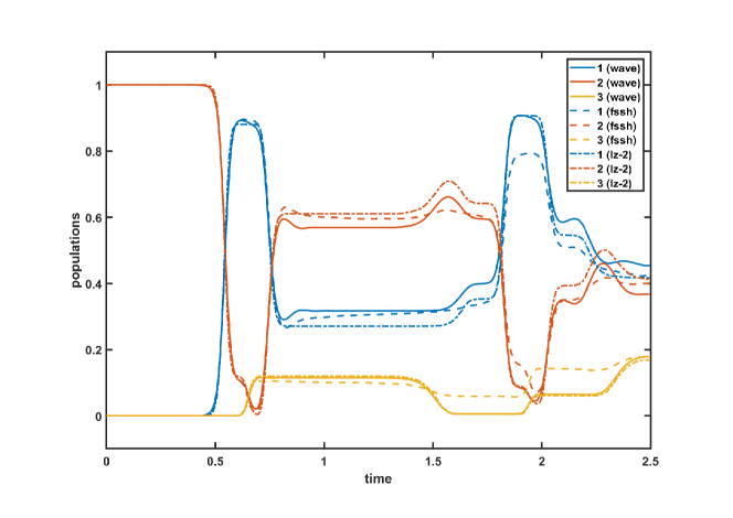
Figure 2: Population dynamics for the Hamiltonian of Eq. (9): Population of the three adiabatic states (numbered according to ascending energy) for fully quantum-mechanical (full curves) versus quantum-mechanical propagations. Fewest switches surface hopping (dashed curves) and single switch surface hopping (dash-dotted curves). Generated with WavePacket option: plots.expect = vis.expect

As an example we show in Fig. 2 the population transfer for the system introduced in Sec. III, comparing numerically exact quantum dynamics with SHT approximations. While the FSSH algorithm reproduces the first population transfer ($2\rightarrow 1$) practically exactly, there are minor deviations of the populations after the second transfer ($2\rightarrow 1$). A closer inspection shows that these discrepancies are due to geometric phase effects. Nonetheless, also the shape of the (here not very pronounced) Stueckelberg oscillations is at least qualitatively reproduced.

V.3 Single switch surface hopping

The second family of SHT approaches implemented in WavePacket is not requiring integration of quantum state vectors along each of trajectory. These SHT algorithms are referred to as “single switch surface hopping” (SSSH) because the hopping probability is only evaluated once for every passage of transition regions, typically intersections of adiabatic potential energy surfaces. Assuming a locally linear double cone topology of the surfaces in these regions, the transition probabilities in SSSH algorithms are based on variants of Landau-Zener (LZ) formulae Lasser et al. (2007); Lasser and Swart (2008); Fermanian Kammerer and Lasser (2008); Belyaev and Lebedev (2011); Belyaev et al. (2014, 2015).

The first single switch variant implemented in WavePacket is accessed by

time.hop = hop.lz_1;

Essentially, it represents the conventional analytic LZ result. In a diabatic representation, the probability for hopping from state $m$ to state $n$ is given by

$$\gamma_{m\rightarrow n}=\exp\left(-2\pi\frac{V_{nm}^{2}}{\frac{d}{dt}|V_{nn}-V_{mm}|}\right)$$ (21)

where the time-derivative of the diabatic energy gap is obtained by finite differencing along the trajectories. Note that the formula is evaluated only at the center of a nonadiabatic region, i. e. where diabatic potentials intersect each other. In an adiabatic formulation, the hopping probability yields Fermanian Kammerer and Lasser (2008); Belyaev and Lebedev (2011)

$$\gamma_{m\rightarrow n}=\exp\left(-\frac{\pi}{4}\frac{Z_{nm}}{|\frac{P}{M}\cdot F_{nm}|}\right)$$ (22)

Also this formula is applied only once for each nonadiabatic region, namely whenever an eigenvalue gap $Z_{nm}\equiv|E_{n}-E_{m}|$ becomes minimal along an individual classical trajectory.

The necessity to calculate NAC vectors $\mathbf{F}$ is circumvented elegantly in the second single switch variant implemented in WavePacket which can be invoked by

time.hop = hop.lz_2;

This approach is available in an adiabatic picture only, and the probability for surface hopping is expressed only in terms of adiabatic energy gaps and second time derivatives thereof Belyaev and Lebedev (2011); Belyaev et al. (2014, 2015)

$$\gamma_{m\rightarrow n}=\exp\left(-\frac{\pi}{2}\sqrt{\frac{Z_{nm}^{3}}{\frac{d^{2}}{dt^{2}}Z_{nm}}}\right)$$ (23)

which again is evaluated only at local minima of energy gaps $Z_{nm}$. This formulation offers the unique advantage of not requiring nonadiabatic coupling information any more, which makes this method not only more efficient than any of the above methods but it is also in line with the application of electronic structure methods in molecular sciences where often only adiabatic energy surfaces $\mathbf{E}$ are available.

The accuracy of the SHT algorithm based on Eq. (23) is also shown in Fig. 2. For the test system of Sec. III, SSSH and FSSH reproduce the population transfer from numerically exact quantum dynamics with roughly equal quality. However, the weak Stueckelberg oscillation structure is absent in the SSSH results, due to the semi-classical nature of the underlying LZ approximation.

VI Summary and outlook

The present version 6.0.2 of WavePacket represents a major step forward from previous versions 5.x of that software, with the main new feature being the addition of classical trajectories and surface hopping techniques. To the best of our knowledge, WavePacket is the only software package that can be used for fully classical, mixed quantum-classical, and fully quantum-mechanical propagations of physical/chemical systems on an equal footing, i. e., for the same Hamiltonian, initial conditions and time stepping. On the one hand, for low–dimensional systems this allows for a direct comparison of classical versus quantum dynamics which can be used, e. g., to identify quantum effects and assess their importance for various simulation tasks. On the other hand, the quantum-classical propagation techniques allow to substantially increase the number of degrees of freedom that can be treated with WavePacket, at least for systems with a clear separation of fast and slow coordinates where quantum effects can be restricted to the former ones.

Technically, these changes of WavePacket have been made possible by a major rewrite in an object-oriented manner. While the oldest versions of our software package were still written in a relatively traditional, completely procedural way, the introduction of generalized DVR/FBR methods in version 4.5 led us to make (limited) use of the object-oriented features offered by Matlab. These approaches have now been extended to large parts of the code of version 6.0.2. In particular, by introducing the WavePacket main classes wave and traj, the function qm_propa has been made polymorph, i. e., being able to propagate quantum and classical objects alike. Along these lines, further extensions of the software package will be relatively easy to realize. This includes the main classes ket and rho for the implementation of quantum state vectors and density matrices in eigen representation which are currently under development. Future releases of WavePacket will also include class definitions implementing various semi-classical approaches based on Gaussian packets in phase space Horenko et al. (2002b); Lasser and Sattlegger (2017); Buchholz et al. (2018). Of particular interest will be nonadiabatic extensions of Gaussian propagation methods, such as the multiple spawning technique Ben-Nun and Martínez (2002), surface hopping Gaussian propagations Horenko et al. (2002a), or adaptive variants thereof Horenko et al. (2004).

In addition to the WavePacket main classes described above, also many other parts of our software package are now based on Matlab classes. Currently there are almost 100 class definitions which are used especially where choices are to be made for a user-defined setup of the system to be simulated. As has been shown in Sec. III, these options encompass DVRs/FBRs, kinetic and potential energy operators, initial states, propagators, visualization types, etc.. This also includes the choice of different types of SHT techniques which have recently been added to our software. It is planned to add more variants here to keep up with the recent progress in surface hopping Wang et al. (2016). In summary, the introduction of object-oriented techniques has been instrumental in achieving a fully modular design, thus making the codes much more flexible, in order to cover the growing diversity of physical/chemical systems that can be simulated with WavePacket.

Appendix A Computation of adiabatic forces and NAC vectors

In order to perform classical or quantum-classical dynamics in the adiabatic picture, the gradients of the adiabatic potentials are necessary. After diagonalizing the diabatic potential matrix

$$\mathbf{E}(R)=\mathbf{U}(R)^{T}\mathbf{V}(R)\mathbf{U}(R)$$ (24)

and storing its eigenvectors $u_{i}(R)$, WavePacket evaluates the gradients of the adiabatic potential energy surfaces by applying the Hellmann-Feynman theorem

$$\nabla_{R_{k}}E_{i}(R)=u_{i}(R)^{T}\left(\nabla_{R_{k}}\mathbf{V}(R)\right)u_{i}(R)$$ (25)

where the knowledge of the gradient of the diabatic potential matrix is required.

For the adiabatic variant of the FSSH algorithm, see Eq. (20), the hopping probability depends on the NAC vectors. By using the eigenvectors of the diabatic potential matrix, these vectors can be represented by

$$F^{k}_{ij}(R)=u_{i}(R)^{T}\nabla_{R_{k}}u_{j}(R).$$ (26)

However, this representation depends on the gradients of the eigenvectors which, typically, are not available. To avoid this problem, WavePacket uses the following formula for the NAC vectors

$$F^{k}_{ij}(R)=\frac{u_{i}(R)^{T}\left(\nabla_{R_{k}}\mathbf{V}(R)\right)u_{j}(R)}{E_{j}(R)-E_{i}(R)}$$ (27)

where, again, the knowledge of the gradient of the diabatic potential matrix is required.

Average computation times of WavePacket on a Macbook computer (1.3 GHz Intel Core i5 processor; 4 GB 1600 MHz DDR3 memory) are shown in Fig. 3. The measured times are for the case of adiabatic FSSH simulations in two dimensions, generalizing the example defined in Sec. III to a variable number $\nu$ of coupled states. First, we note that for $\nu=2$, the diagonalizations as well as the calculations of forces and NAC vectors are carried out analytically which is the reason why these calculations are very fast. Hence, we will consider only the data for $\nu>2$ in the following. There, the time for diagonalization (24) rises only very slowly with increasing $\nu$ which is due to the sparsity of matrix $\mathbf{V}$ for our example. The other curves, however, behave as expected, i. e., the effort to calculate adiabatic forces (25) as well as $\mathbf{F}$ vectors (27) for a single pair of adiabatic states scales as $\mathcal{O}(\nu^{2})$. Consequently, the cost to calculate the whole matrix of first order NAC vectors scales as $\mathcal{O}(\nu^{4})$. Also shown is the time used for the numerical TDSE integrator (based on diagonalization of $\mathbf{V}$) which scales as $\mathcal{O}(\nu^{3})$. Note that the latter two contributions are omitted in SSSH simulations which makes them considerably faster than FSSH for approximately $\nu>10$.

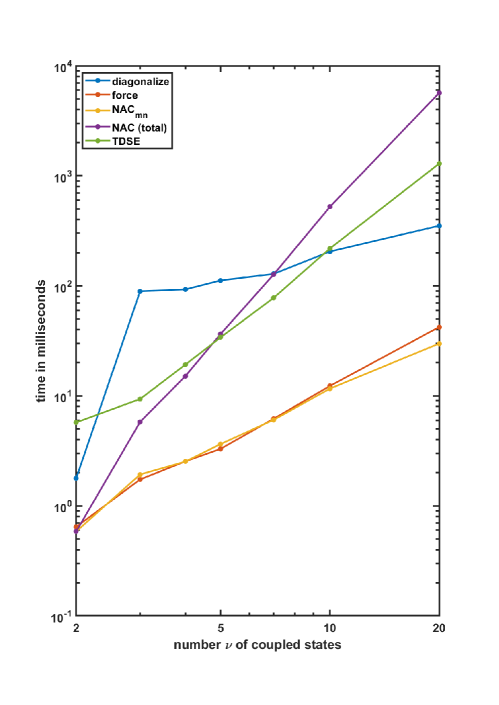
Figure 3: Double-logarithmic representation of WavePacket computational time for diagonalization of $\mathbf{V}$ and calculation of adiabatic forces as well as of NAC vectors $\mathbf{F}$ in FSSH for 2 dimensions and varying number $\nu$ of coupled channels. For 100 time steps of an FSSH simulation with 1000 trajectories in adiabatic representation.

References

- Zewail (2000) A. H. Zewail, The Journal of Physical Chemistry A 104, 5660 (2000).
- May and Kühn (2000) V. May and O. Kühn, Charge and Energy Transfer Dynamics in Molecular Systems (Wiley, Berlin, 2000).
- Tannor (2004) D. Tannor, Introduction to Quantum Mechanics. A Time-Dependent Perspective (University Science Books, Sausalito, 2004).
- Beck et al. (2000) M. H. Beck, A. Jäckle, G. A. Worth, and H.-D. Meyer, Physics Reports 324, 1 (2000).
- Khan et al. (2014) B. A. Khan, S. Sardar, P. Sarkar, and S. Adhikari, The Journal of Physical Chemistry A 118, 11451 (2014).
- Johansson et al. (2013) J. R. Johansson, P. D. Nation, and F. Nori, Computer Physics Communications 184, 1234 (2013).
- Mendl (2011) C. B. Mendl, Computer Physics Communications 182, 1327 (2011).
- Machnes et al. (2011) S. Machnes, U. Sander, S. J. Glaser, P. D. Fouqui, A. Gruslys, and S. Schirmer, Physical Review A 84, 022305 (2011).
- Schmidt and Lorenz (2017) B. Schmidt and U. Lorenz, Computer Physics Communications 213, 223 (2017).
- Schmidt and Hartmann (2018) B. Schmidt and C. Hartmann, Computer Physics Communications 228, 229 (2018).
- Wang and Thoss (2003) H. Wang and M. Thoss, The Journal of Chemical Physics 119, 1289 (2003).
- Tully (1990) J. C. Tully, The Journal of Chemical Physics 93, 1061 (1990).
- Barbatti et al. (2014) M. Barbatti, M. Ruckenbauer, F. Plasser, J. Pittner, G. Granucci, M. Persico, and H. Lischka, Wiley Interdisciplinary Reviews: Computational Molecular Science 4, 26 (2014).
- Mitrić et al. (2009) R. Mitrić, J. Petersen, and V. Bonačić-Koutecký, Physical Review A - Atomic, Molecular, and Optical Physics 79, 1 (2009).
- Richter et al. (2011) M. Richter, P. Marquetand, J. González-Vázquez, I. Sola, and L. González, Journal of Chemical Theory and Computation 7, 1253 (2011).
- Mai et al. (2018) S. Mai, P. Marquetand, and L. González, Wiley Interdisciplinary Reviews: Computational Molecular Science 8, e1370 (2018).
- Tully (2012) J. C. Tully, The Journal of Chemical Physics 137, 22A301 (2012).
- Wang et al. (2016) L. Wang, A. Akimov, and O. V. Prezhdo, The Journal of Physical Chemistry Letters 7, 2100 (2016).
- Subotnik et al. (2016) J. E. Subotnik, A. Jain, B. Landry, A. Petit, W. Ouyang, and N. Bellonzi, Annual Review of Physical Chemistry 67, 387 (2016).
- Lasser et al. (2007) C. Lasser, T. Swart, and S. Teufel, Communications in Mathematical Sciences 5, 789 (2007).
- Lasser and Swart (2008) C. Lasser and T. Swart, The Journal of Chemical Physics 129, 034302 (2008).
- Fermanian Kammerer and Lasser (2008) C. Fermanian Kammerer and C. Lasser, The Journal of Chemical Physics 128, 144102 (2008).
- Belyaev and Lebedev (2011) A. K. Belyaev and O. V. Lebedev, Physical Review A 84, 014701 (2011).
- Belyaev et al. (2014) A. K. Belyaev, C. Lasser, and G. Trigila, The Journal of Chemical Physics 140, 224108 (2014).
- Belyaev et al. (2015) A. K. Belyaev, W. Domcke, C. Lasser, and G. Trigila, The Journal of Chemical Physics 142, 104307 (2015).
- Giustino (2017) F. Giustino, Reviews of Modern Physics 89, 1 (2017), eprint 1603.06965.
- Viel and Eisfeld (2004) A. Viel and W. Eisfeld, The Journal of Chemical Physics 120, 4603 (2004).
- Eisfeld and Viel (2005) W. Eisfeld and A. Viel, The Journal of Chemical Physics 122, 204317 (2005).
- Domcke et al. (2004) W. Domcke, D. R. Yarkony, and H. Köppel, eds., Conical Intersections. Electronic Structure, Dynamics and Spectroscopy, vol. 15 of Advanced Series in Physical Chemistry (World Scientific, Singapore, 2004).
- Baer (2006) M. Baer, Beyond Born–Oppenheimer (Wiley-VCH, Hoboken, New Jersey, 2006).
- Panati et al. (2007) G. Panati, H. Spohn, and S. Teufel, Mathematical Modelling and Numerical Analysis 41, 297 (2007).
- Light and Carrington (2000) J. C. Light and T. Carrington, Advances in Chemical Physics 114, 263 (2000).
- Leforestier et al. (1991) C. Leforestier, R. Bisseling, C. Cerjan, M. Feit, R. Friesner, A. Guldberg, A. Hammerich, G. Jolicard, W. Karrlein, H.-D. Meyer, et al., Journal of Computational Physics 94, 59 (1991).
- Askar and Cakmak (1978) A. Askar and A. S. Cakmak, Journal of Chemical Physics 68, 2794 (1978).
- Fleck et al. (1976) J. A. Fleck, J. R. Morris, and M. D. Feit, Applied Physics 10, 129 (1976).
- Feit et al. (1982) M. Feit, J. Fleck, Jr, and A. Steiger, Journal of Computational Physics 47, 412 (1982).
- Tal-Ezer and Kosloff (1984) H. Tal-Ezer and R. Kosloff, Journal of Chemical Physics 81, 3967 (1984).
- Kapral and Ciccotti (1999) R. Kapral and G. Ciccotti, The Journal of Chemical Physics 110, 8919 (1999).
- Horenko et al. (2002a) I. Horenko, C. Salzmann, B. Schmidt, and C. Schütte, The Journal of Chemical Physics 117, 11075 (2002a).
- Tully and Preston (1971) J. C. Tully and R. K. Preston, The Journal of Chemical Physics 55, 562 (1971).
- Subotnik et al. (2013) J. E. Subotnik, W. Ouyang, and B. R. Landry, The Journal of Chemical Physics 139, 214107 (2013).
- Verlet (1967) L. Verlet, Physical Review 159, 98 (1967).
- Frenkel and Smit (2002) D. Frenkel and B. Smit, Understanding Molecular Simulation (Academic Press, San Diego, 2002).
- Beeman (1976) D. Beeman, Journal of Computational Physics 20, 130 (1976).
- Yoshida (1990) H. Yoshida, Physics Letters A 150, 262 (1990).
- Horenko et al. (2002b) I. Horenko, B. Schmidt, and C. Schütte, The Journal of Chemical Physics 117, 4643 (2002b).
- Lasser and Sattlegger (2017) C. Lasser and D. Sattlegger, Numerische Mathematik 137, 119 (2017).
- Buchholz et al. (2018) M. Buchholz, E. Fallacara, F. Gottwald, M. Ceotto, F. Grossmann, and S. D. Ivanov, Chemical Physics (2018).
- Ben-Nun and Martínez (2002) M. Ben-Nun and T. J. Martínez, Advances in Chemical Physics 121, 439 (2002).
- Horenko et al. (2004) I. Horenko, M. Weiser, B. Schmidt, and C. Schütte, The Journal of Chemical Physics 120, 8913 (2004).