Hunting for the Dark Matter Wake Induced by the Large Magellanic Cloud

Abstract

Satellite galaxies are predicted to generate gravitational density wakes as they orbit within the dark matter (DM) halos of their hosts, causing their orbits to decay over time. The recent infall of the Milky Way’s (MW) most massive satellite galaxy, the Large Magellanic Cloud (LMC), affords us the unique opportunity to study this process in action. In this work, we present high-resolution ($m_{dm}=4\times 10^{4}\rm{M_{\odot}}$) $N$-body simulations of the MW-LMC interaction over the past 2 Gyr. We quantify the impact of the LMC’s passage on the density and kinematics of the MW’s DM halo and the observability of these structures in the MW’s stellar halo. The LMC is found to generate a pronounced wake, which we decompose in Transient and Collective responses, in both the DM and stellar halos. The wake leads to overdensities and distinct kinematic patterns that should be observable with ongoing and future surveys. Specifically, the Collective response will result in redshifted radial velocities of stars in the north and blueshifts in the south, at distances $>$45 kpc. The Transient response traces the orbital path of the LMC through the halo (50-200 kpc), resulting in a stellar overdensity with a distinct, tangential kinematic pattern that persists to the present day. The detection of the MW’s halo response will constrain the infall mass of the LMC and its orbital trajectory, the mass of the MW, and it may inform us about the nature of the DM particle itself.

1 Introduction

Perturbations induced by orbiting satellite galaxies within the dark matter (DM) halos of their hosts have been studied since the seminal work of Chandrasekhar (1943). It has been recognized that satellite galaxies generate density wakes by direct gravitational scattering of particles that pull back on the satellite, causing the satellite to lose angular momentum and energy in a process referred to as dynamical friction (Binney & Tremaine, 2008).

It was later discovered that such local scattering is a manifestation of the resonant nature of the system (Tremaine & Weinberg, 1984). In particular, White (1983) and Weinberg (1998a) found that, on global scales, resonances between orbital frequencies of the DM particles in the halo and the satellite’s orbital frequency can effectively transfer angular momentum and energy from the satellite to the DM halo. These resonances produce overdensities and underdensities, which also consequently affect the kinematics of the DM halo.

During the first passage of a satellite around a host galaxy, the frequency of the satellite’s orbit is continuous, and it has a broad range of frequencies that resonate with those of the DM particles of the host galaxy. These resonances produce the classical ‘conic’ wake that trails the satellite described in Chandrasekhar (1943). However, as the satellite continues orbiting around the host galaxy, its orbit’s frequencies range gets narrower and hence it resonates with particular frequencies of the DM particles. As a consequence, the classical ‘conic’ wake weakens and overdensities in other regions of the DM halo start to take place. In this paper, we will refer to these density and kinematic perturbations as the Transient response and Collective response. The Transient response corresponds to the classical Chandrasekhar’s wake, which trails the satellite galaxy. The Collective response corresponds to those overdensities and underdensities not trailing the satellite, generated by the narrow range resonances after the first passage.

For a detailed and comprehensive review of these resonant processes, we refer the reader to Choi et al. (2009), where a theoretical framework using perturbation theory is derived and compared to $N$-body simulations to investigate the resonances induced by a satellite in the DM halo of its host. Choi et al. (2009) found that the location of the resonances within the halo is dictated by the orbital frequency and trajectory of the satellite. As such, detailed studies of the DM halo wake produced by a particular satellite must accurately account for the satellite’s exact orbit.

In addition to the DM halo responses, the gravitational acceleration induced by a satellite galaxy will also offset the DM halo cusp of the host galaxy from the original DM halo center of mass (COM) (Choi et al., 2009; Ogiya & Burkert, 2016). Consequently, the orbital barycenter of the host galaxy will move (Gómez et al., 2015). Accounting for these effects is crucial to properly interpret astrometric data of observed satellites, streams and globular clusters. For example, Gómez et al. (2015) showed that accounting for the Milky Way’s (MW) barycenter motion due to the gravitational pull from the Large Magellanic Cloud (LMC) can reconcile the mismatch between observations and simulations of the morphology of the Sagittarius Dwarf spheroidal galaxy (Sgr dSph) stellar stream, without invoking a triaxial DM halo model.

In reality, the MW’s halo is embedded with multiple substructures, such as satellite galaxies, globular clusters, and smaller DM subhalos, that induce localized perturbations to the DM and stellar halo. For example, Loebman et al. (2018) find disturbances in the velocity distribution of stars along sightlines that pass through individual satellite galaxies. These velocity changes manifest as “dips” in the anisotropy parameter profile, $\beta(r)$ defined as

$$\beta=1-\frac{\sigma_{t}^{2}}{2\sigma_{r}^{2}},$$ (1)

where $\sigma_{r}$ and $\sigma_{t}$ are the radial and tangential velocity dispersions, respectively. Positive values of $\beta$ correspond to radially biased orbits, while negative values correspond to tangentially biased orbits.

In corroboration, Cunningham et al. (2019) used the Latte cosmological-zoom simulations of two MW-like galaxies (Wetzel et al., 2016) to show that substructure can cause $\beta$ to vary locally from -1 to 1. However, these perturbations do not fundamentally alter the kinematics of the entire MW stellar halo or DM halo itself, but are instead localized perturbations associated with substructure that only span a few kpc. In addition to the variations in $\beta$ caused by substructure, Loebman et al. (2018) found a long-lived tangential bias in the $\beta$ profile of galaxies that have undergone a recent major merger. Moreover, “$\beta$ dips” can correspond to breaks in the stellar density profile resulting from the assembly history of a galaxy (Rashkov et al., 2013). While none of these studies were specific to the MW system, they do strongly suggest that the LMC should cause a potentially significant observable kinematic signature in the stellar halo. Indeed, the LMC is likely inducing significant perturbations to the MW’s disk (Laporte et al., 2016, 2018a) and stellar streams, such as Tucana III (Erkal et al., 2018) and the Orphan Stream (Erkal et al., 2019).

The LMC is the most massive satellite galaxy of the MW and is most likely on a highly eccentric orbit, only just past its first pericentric approach to our Galaxy (Besla et al., 2007; Kallivayalil et al., 2013). Patel et al. (2017b) found using the Illustris simulation that is extremely rare to find a high-speed, massive ($\sim$10¹¹ M_⊙) satellite in close proximity to a massive host at $z=0$ in cosmological simulations, see also (Boylan-Kolchin et al., 2011; Busha et al., 2011; Cautun et al., 2019).

As such, studying the DM halo wake induced by the LMC in a cosmological context remains a challenge and is beyond the scope of this paper . Instead, we construct detailed $N$-body models of the LMC’s recent orbit, from its first crossing of the MW’s virial radius, $\sim$2 Gyr ago, to the present day. With controlled numerical experiments, we can predict the general form and locations of perturbations in the kinematics of the MW’s stellar halo and ultimately link those perturbations to the passage of the LMC and its induced wake within the MW’s DM halo. These constrained simulations allow us to match the LMC’s current 6D phase-space properties within 2$\sigma$ of observations (see also Laporte et al., 2018a), which is not currently possible with cosmological simulations.

The amplitude of the DM wake induced by typical MW satellite galaxies ($M_{halo}\sim 10^{9}-10^{10}$ M_⊙) is expected to be much smaller than that of the LMC ($M_{halo}\sim 10^{11}$ M_⊙). We will illustrate this point by comparing the properties of the LMC’s DM wake to that of the next most massive perturber, the Sagittarius dwarf galaxy (Laporte et al., 2018b). Indeed, DM wakes induced by massive orbiting satellites are identifiable in cosmological-zoom-in simulations of MW-like galaxies (Gómez et al., 2016), despite the presence of multiple smaller orbiting bodies. In such cases, DM wakes are found to not only affect the DM and stellar halo density and kinematics but also the structure of the galactic disk (e.g. Weinberg & Blitz, 2006; Gómez et al., 2016, 2017). However, note that perturbations in the halo from the combination of multiple subhalos can be coupled in nontrivial ways (Weinberg & Katz, 2007).

Critically, in this study, we will assess the ability of current and future surveys to identify the signatures of the DM wake generated by the LMC within the MW’s stellar halo. Current and near-future observational studies of the kinematics and structure of the stellar halo (Gaia, RAVE, H3, DES, DESI, APOGEE, GALAH, LAMOST, LSST, 4MOST, and WEAVE) will reveal the structure and the kinematic state of the stellar halo of the MW. Soon, the phase-space information, i.e., distances, proper motions and radial velocities, of millions of stars out to at least $100$ kpc will be known, in addition to that of other halo tracers, such as satellites and globular clusters.

Ultimately, the phase-space information of halo tracers can inform us about the underlying DM potential, the total mass, and the accretion history of the MW (Johnston et al., 2008; Helmi, 2008; Gómez et al., 2010; Carlin et al., 2016). However, the LMC is a major perturber to the MW’s halo that has not yet been properly accounted for in such studies. This study of the kinematic and density perturbations induced by the LMC is essential to properly compute the uncertainty in current MW mass estimates. Strong variations in the kinematics of the stellar and DM halos (i.e. in $\beta$) across the sky will cause variations in estimates of the mass of the MW inferred through Jeans modeling (e.g., Watkins et al., 2010). Furthermore, given the lack of 6D phase-space information in the outer regions of the stellar halo, it is common to extrapolate DM profiles to large radii using constraints within the inner 50 kpc. However, the LMC can strongly modify the distribution of mass in the outer halo - the resulting asphericity will also affect MW mass estimates (Wang et al., 2018).

Specifically, we seek to answer the following questions: are the phase-space properties of the stellar halo conserved in the presence of the LMC? What are the kinematic signatures of the DM halo wake induced by the LMC? Can we identify the LMC’s DM wake and track the past orbit of the LMC through the stellar halo? Addressing these questions is essential to properly interpreting the data from current and upcoming high-precision astrometric surveys (Dey et al., 2019; Sanderson et al., 2019; Li et al., 2019) and may provide new cosmological tests of the total DM mass of the LMC and MW and the nature of the DM particle itself.

The structure of this paper is as follows: in §2, we discuss current estimates for the mass of the LMC. §3 describes the numerical methods and initial conditions. In §4, we discuss the main results of our simulations, focusing on the density and the kinematics of the Transient and Collective response induced within the stellar and DM halos of the MW. In §5 we discuss the observability of our findings, given current and upcoming surveys. In §6 we discuss: the convergence of our simulations; how our results scale as a function of the LMC mass; comparisons between the DM wake produced by the LMC against that of Sgr; how the Transient response can be distinguished from stellar debris associated with the Magellanic Stream; and the prospects for studying the nature of DM using the LMC’s DM wake. We conclude in §7.

2 The mass of the LMC

The response of the MW’s DM halo and corresponding perturbations to the kinematics of the MW’s stellar halo will depend on the total mass of the LMC. Moreover, owing to dynamical friction, the orbital history of the LMC also strongly depends on its mass (Kallivayalil et al., 2013). However, the LMC’s mass is uncertain within a factor of $\sim$10. Many theoretical models of the Magellanic System have assumed low halo masses for the LMC ( $\sim 10^{10}$ M_⊙, e.g. Gardiner & Noguchi, 1996; Connors et al., 2006; Yoshizawa & Noguchi, 2003; Diaz & Bekki, 2011; Guglielmo et al., 2014). However, massive LMC-halo models ($10^{11}$M_⊙) have also been shown to reproduce several observations, such as the global properties of the Magellanic System (Besla et al., 2010, 2012, 2013; Salem et al., 2015; Pardy et al., 2018), the morphology of the MW’s HI disk and its resulting line of nodes (Weinberg & Blitz, 2006; Laporte et al., 2018a), and in the misalignment of the velocity vectors of the Orphan stream (Erkal et al., 2019). In addition, there are a mounting number of arguments that together strongly support a high infall mass for the LMC, $\rm{M_{vir}}>8\times 10^{10}$ M_⊙ as listed below.

1. Rotation Curve: van der Marel & Kallivayalil (2014) derived the rotation curve of the LMC using the HST proper motions of 22 stars with known line-of-sight velocities. The derived rotation curve peaks at $91.7\pm 18.8$km s^-1 at $8.7$ kpc, which implies an enclosed dynamical mass of $\rm{M(<8.7)}=1.7\times 10^{10}\rm{M_{\odot}}$. This is a strict minimum mass for the LMC, which is already at odds with many existing theoretical models.

2. Extent of the LMC’s Stellar Disk: The stellar disk of the LMC has been observed out to a radius of $\sim 19$ kpc (Saha et al., 2010; Mackey et al., 2016; Nidever et al., 2019) from the LMC’s optical center. This indicates that the LMC is not tidally truncated at $8.7$ kpc (Besla et al., 2016). As such, the mass of the LMC must be larger than the dynamical mass estimate, within 8.7 kpc, of $1.7\times 10^{10}\rm{M_{\odot}}$. If the rotation curve remains flat to $\sim 19$ kpc the enclosed mass is $\sim 3.7\times 10^{10}\rm{M_{\odot}}$. On the other hand, if one assumes that the tidal radius of the LMC is $19$ kpc, one can back out the mass of the LMC. Assuming an enclosed MW halo mass within $50$ kpc of $\sim 5\times 10^{11}\rm{M_{\odot}}$ (Kochanek, 1996), the minimum mass of the LMC must be $8.3\times 10^{10}\rm{M_{\odot}}$ at the present day.

   But the LMC does not illustrate clear evidence for tidal truncation, suggesting its infall mass could be much larger. In this study, we assume a minimum mass of the LMC at infall of $8\times 10^{10}\rm{M_{\odot}}$.

3. Cosmological Expectations: The total stellar mass of the LMC is $3.2\times 10^{9}$ M_⊙ (van der Marel et al., 2009). Using abundance matching, a statistical technique used to assign a DM halo mass to a galaxy of a given stellar mass, the total mass of the LMC, prior to accretion by the MW, should be $\sim 1.6\times 10^{11}$ M_⊙ (Behroozi et al., 2010; Guo et al., 2010; Moster et al., 2010).

   Similarly, if a typical baryon fraction of $3\%$ (appropriate for spiral galaxies) is assumed, the total mass of the LMC before accretion should be $\sim 10^{11}$ M_⊙. These calculations indicate that the LMC was likely quite massive at infall.

   HST proper motions indicate that the LMC was likely recently captured ($<2$ Gyr ago) (Kallivayalil et al., 2013). This first infall scenario is the cosmologically preferred orbital history for massive satellites of MW-mass hosts at z=0 (Boylan-Kolchin et al., 2011; Busha et al., 2011; González et al., 2013; Patel et al., 2017a). In such a scenario, the LMC should retain a significant fraction of its infall mass at the present day (e.g., Sales et al., 2011).

4. Satellites of the LMC:. The presence of the SMC and potentially multiple smaller satellites companions (D’Onghia & Lake, 2008; Jethwa et al., 2016; Kallivayalil et al., 2018), also indicates that the LMC must have been relatively massive at infall. In particular, satellites with stellar masses similar to the LMC that also have an SMC companion usually reside in DM halos with a mass of $\rm{M}_{200}=3.4^{+1.8}_{-1.2}\times 10^{11}\rm{M_{\odot}}$ (Shao et al., 2018). This high mass is also supported by studies of cosmological dwarf galaxy pairs in the field (Besla et al., 2018).

5. Timing argument: The mass of galaxies in the Local Group can be derived using the timing argument. This method compares the galaxies’ currently observed positions and velocities to the solution of their equations of motion in an expanding universe (Kahn & Woltjer, 1959; Lynden-Bell, 1981; Sandage, 1986; Partridge et al., 2013; Peñarrubia et al., 2014). These equations can be solved if the potential, the rate at which the universe is expanding, and the time since the galaxies separated ($\approx 13.7$ Gyr, assumed to be the age of the universe) are known. Peñarrubia et al. (2016) applied a Bayesian inference method to constrain the total mass of the LMC using the timing argument. They found that the LMC’s total virial mass before infall is most likely $\rm{M}_{LMC}=2.5^{+0.9}_{-0.8}\times 10^{11}$ M_⊙ (see also, Peebles, 2010). We use this estimate as an upper limit on the mass of the LMC. Our team has recently illustrated that such a high LMC mass is able to induce a strong warp in the outer disk. However, it does not cause significant kinematic perturbations to the MW’s disk in the solar neighborhood that violate observational constraints (Laporte et al., 2018a).

6. Perturbations to Stellar Streams: Recently, Koposov et al. (2019) identified prominent twists in the shape of the Orphan Stream on the sky and nonzero motion in the across-stream direction. Erkal et al. (2019) then illustrated that the misalignment between the debris track and the streaming velocity cannot be reproduced in a static gravitational potential, but is instead best explained by perturbations from the LMC, provided it had an infall mass of $1.3^{+0.27}_{-0.24}\times 10^{11}$ M_⊙.

Given the above arguments, we choose a range of $8-25\times 10^{10}\rm{M_{\odot}}$ for the LMC’s virial mass at the time it first crossed the virial radius of the MW, noting that it could have been larger. We then simulate the evolution of the LMC to its present location on an orbit consistent with the latest HST proper motions of Kallivayalil et al. (2013). This is the first study of the global impact of such high LMC masses on the MW’s stellar and DM halo, mapping its the full extent of the wake out to 200 kpc.

3 Numerical Methods

The $N$-body simulations were carried out with the Tree Smoothed Particle Hydrodynamics code Gadget-3 (Springel et al., 2008), which is a modified version of Gadget-2 (Springel, 2005) with an improved gravity solver. We use the publicly available code GalIC (Yurin & Springel, 2014) to generate the initial conditions for the MW and the LMC.

3.1 Galaxy Models

Table 1 summarizes the parameters of the adopted MW model. Our MW model has a virial mass of $\rm{M}_{vir}=1.2\times 10^{12}$ M_⊙ (McMillan, 2017). This is defined as the mass enclosed within the virial radius $R_{vir}$, where $R_{vir}$ encloses an overdensity of $\Delta_{vir}=357$. That is, $\rho_{vir}=\Delta_{vir}\Omega_{m}\rho$, where $\rho$ is the average density of the universe. We do not vary the mass of the MW in this study, as the first infall orbits for the LMC are not recovered for massive MW models ($\rm{M}_{vir}>1.5\times 10^{12}$M_⊙) and the LMC orbit has behaved similarly in lower-mass MW models over the past 1-2 Gyr (Kallivayalil et al., 2013; Gómez et al., 2015).

The DM halo of the MW is represented by a Hernquist profile (Hernquist, 1990), where the scale length $r_{a}$ was chosen in order to guarantee that the enclosed mass at the virial radius is the same as that of the equivalent NFW profile (for details of this procedure, see the appendix of van der Marel et al. (2012)). Note that GalIC uses quantities evaluated at $R_{200}$ as input parameters, which is the radius at which the enclosed density is 200 times the critical density of the universe. We have changed these definitions to virial quantities in GalIC in order to ensure equivalence between the NFW density profile and the Hernquist profile.

The halo spin parameter $\lambda=0.027$ and concentration are consistent with typical MW-like DM halos in cosmological simulations (Klypin et al., 2011). We adopt two different internal kinematic profiles for the MW’s DM halo, represented by the anisotropy parameter $\beta$ (see §3.2 for a detailed description).

The disk of the MW is represented by an exponential profile and the stellar bulge of the MW is modeled using a Hernquist profile. The stellar and DM particle mass are both $m_{p}=4\times 10^{4}$ M_⊙. The adopted MW disk, bulge, and halo parameters are within $2\sigma$ of the best-fitting MW parameters in McMillan (2017), such that the rotation curve reaches a peak of $\sim$240 km/s. We have included a disk and bulge in order to ensure that the potential is realistic in the inner regions of the halo ($<$ 30 kpc) and to accurately track the COM of the system.

Note that our simulations have small discreteness and can accurately capture distortions to the LMC’s DM distribution. While small-scale resonances can be affected by discreteness noise, we are interested in structures over larger scales (several kpc). In general, the number of particles used in our simulations is six orders of magnitude greater than the regimes where these effects take place, as discussed in van den Bosch et al. (2018) and van den Bosch & Ogiya (2018).

MW Component	Parameter	Value
DM halo	Mvir, M200 $[\times 10^{12}\rm{M_{\odot}}]$	$1.2,1.03$
	$R_{vir},R_{200}$ [kpc]	$279,208$
	concentration $c_{vir}$	15
	scale length $a_{halo}$ [kpc]	40.82
	DM halo particles	$10^{8}$
	Mass per DM particle [M⊙]	$4\times 10^{4}$
Disk	M${}_{disk}[\times 10^{10}$M${}_{\odot}]$	5.78
	Disk scale length $r_{a}$ [kpc]	3.5
	Disk scale height $r_{b}$ [kpc]	0.5
	Disk particles	1382310
Bulge	M${}_{bulge}[\times 10^{10}\rm{M_{\odot}}]$
	scale length $a_{bulge}$ [kpc]	0.7
	Bulge particles	335220

Table 1: Milky Way Model Parameters Parameters defining the simulated MW. Models 1 and 2 have the same parameters, but are initialized with different anisotropy profiles (§3.2). The MW is modeled using a Hernquist profile to describe the halo and bulge, and an exponential profile for the stellar disk.

For the LMC, we construct four models with total halo masses of $\rm{M}_{vir}=0.8,1.0,1.8,2.5\times 10^{11}$ M_⊙. The bulk of this study will focus on a fiducial LMC model, with a halo mass of $1.8\times 10^{11}$ M_⊙, which is consistent with both models of the Magellanic System on a first infall (Besla et al., 2012, 2013, 2016) and the mean halo mass expected from abundance matching (see § 2). The LMC is modeled using a Hernquist profile to represent the DM halo. We do not include a disk, as we are interested in the impact of the LMC on the MW halo kinematics, where the dominant perturbations comes from the DM halo of the LMC. We identify an adequate Hernquist scale length, $r_{a}$, to guarantee that the circular velocity at $8.7$ kpc is $\sim 92$ km s^-1, as shown in Figure 1. The parameters of the LMC models are presented in Table 2. Note that the DM particle mass of each LMC model matches that of the MW ($m_{dm}=4\times 10^{4}$ M_⊙).

	LMC1	LMC2	LMC3	LMC4
$\rm{M}_{vir},\rm{M}_{200}[\rm{M_{\odot}}\times 10^{10}]$	$8,6.7$	$10,8.35$	$18,14.7$	$25,20.1$
$r_{a}[kpc]$	10.4	12.7	20	25.2
$R_{vir},R_{200}$ [kpc]	113, 83	121, 89	148,108	165, 120
# DM particles [$10^{6}$]	6.66	8.33	15	20.84

Table 2: LMC model parameters: The virial mass $\rm{M}_{vir}$ of the LMC halo for all models is consistent with the arguments given in §2. The values of the Hernquist scale length, $r_{a}$, are chosen to match the observed LMC rotation curve, as illustrated in figure 1. The fiducial LMC model is LMC3.

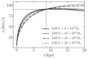
Figure 1: Rotation curves of the four LMC models at infall. The LMC’s DM halo is modeled as a Hernquist profile with a scale factor chosen to match the observed rotation curve. For visual reference, the vertical and horizontal gray dashed lines are at 8.7 kpc and at $91.7\rm{kms^{-1}}$ respectively, illustrating that the models agree with the measurements of van der Marel & Kallivayalil (2014).

3.2 The Milky Way’s Anisotropy Profile, $\beta$

One of the main advantages of using GalIC to generate galaxy initial conditions is that it allows us to specify an initial anisotropy profile, $\beta(r)$, for the DM halo. We build two MW models with different forms for the radial anisotropic profile, $\beta(r)$: (1) Model 1 assumes an isotropic DM halo ($\beta=0$); and (2) Model 2 assumes a radially varying profile (Hansen & Moore, 2006):

$$\beta(r)=-0.5-0.2\alpha(r)\,;\qquad\alpha(r)=\frac{{\rm dln}\,\rho(r)}{{\rm dln}\,r}.$$ (2)

Model 1 allows us to study perturbations from the LMC in the simplest case of an isotropic halo. Once the halo response is understood in this idealized setting, we will use the gained intuition to interpret the perturbations in the more realistic, radially varying profile (Model 2).

Model 2 is radially biased, where the radial dispersion is always larger than the tangential dispersion (see the top right panel of Figure 2). Such a profile agrees with cosmological numerical simulations where both the DM and the stellar halo anisotropy profiles of MW type galaxies increase monotonically with increasing Galactocentric radius (Abadi et al., 2006; Sales et al., 2007).

3.2.1 Stability of the initial $\beta(r)$ profiles

One of our main goals is to study perturbations in the kinematics of the MW’s stellar halo induced by the LMC. As such, we must first test the kinematic stability of the MW models generated with GalIC. We use Gadget-3 to evolve Models 1 and 2 in isolation for 5 Gyr to test the stability of the kinematic and density profile of the MW’s DM halo.

The density profiles show minimum variation over 5 Gyr (bottom panel of Figure 2). On the other hand, $\beta(r)$ is not perfectly stable for the first 2 Gyr (top panel of Figure 2). A “bump” in the $\beta(r)$ profiles appears and evolves with radius over $2$ Gyr. We have identified this to be a numerical artifact of GalIC. However, for both models, the variations are minimal after 2.5 Gyr. As such, we introduce the LMC after the MW has been run in isolation for $\sim$ 2.5 Gyr (purple colors in Figure 2).

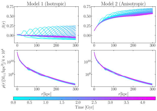
Figure 2: Time evolution of the anisotropy parameter profile, $\beta(r)$ (top), and density profile, $\rho(r)$ (bottom), for the DM halo of Model 1 ($\beta=0$; left panel), and Model 2 ($\beta=-0.5-0.2\alpha$; right panel). The models are evolved in isolation (without the LMC) over 5 Gyr. The timeline is indicated by the color bar (in Gyr). The $\beta$ profile is initially unstable, but variations are minimal after $2.5$ Gyr. In contrast, the density profile remains stable for the duration of the run. As such, we introduce the LMC to the simulation of the MW’s DM halo after $2.5$ Gyr. With these isolated MW halo stability tests, we can confidently isolate the impact of the LMC on the kinematics of the MW’s stellar and DM halo from numerical artifacts.

3.3 Orbit Reconstruction

Using the described MW and LMC models, we set up a suite of $N$-body simulations of the LMC’s orbit within the MW’s DM halo using Gadget-3. Table 3 summarizes the simulation suite. The softening length is $\epsilon=0.08$ kpc, following the criteria of Power et al. (2003) (their equation $15$).

The initial 6D phase-space coordinates of the LMC, i.e. when it first crossed the virial radius of the MW $\sim 2$ Gyr ago, are identified by integrating the orbit of the LMC backwards in time from the present observed position and velocity (Kallivayalil et al., 2013) following the same methodology as in Gómez et al. (2015). We use the dynamical friction equation derived by Chandrasekhar (1943), where we adopt the following Coulomb Logarithm definition following Hashimoto et al. (2003).

$$\centering Ln(\Lambda)=\xi\left(\frac{b_{max}}{b_{min}}\right),\@add@centering$$ (3)

where $b_{max}$ is the Galactocentric position of the LMC, $b_{min}=1.4\,r_{s}$, and $r_{s}$ is the scale radius in kpc. $\xi$ is a free parameter included as a fudge factor in the dynamical friction acceleration adjusted to match the $N$-body orbits.

We start with $\xi=1$ and integrate the orbit of the LMC backwards in time until it reaches the MW’s virial radius, storing the 3D position and velocity vector as a first guess for the initial starting point for the simulated LMC. Then, we run a low-resolution ($m_{dm}=1.2\times 10^{6}\rm{M_{\odot}}$) $N$-body test simulation using the identified first guess initial conditions. We iterate the backwards orbital integration with lower values of $\xi$ until we find good agreement between the analytic and the N-body orbit. This iterative procedure usually requires between two and three iterations. Once an optimal value of $\xi$ is identified for each LMC-MW simulation, the correct initial conditions are found by integrating the observed present values 2 Gyr into the past.

As a result of this iterative procedure, our $N$-body simulations reproduce the magnitude of the LMC’s present-day position and velocity within $2\sigma$ of the observed values ($\Delta r$ and $\Delta v$ in Table 3). Appendix A contains further details of the exact position and velocity vector for each simulated LMC model. In addition, both the velocity and the distance of the LMC at pericenter (50 Myr ago) are within 1$\sigma$ of the analytic expectations ($r_{peri}=48\pm 2.5$ kpc, $v_{peri}=340\pm 19$ km/s) (Salem et al., 2015).

The orbital separation of the LMC COM from that of the MW is illustrated in Figure 3 for all of the $N$-body LMC-MW simulations. The COM position of the MW is computed using disk particles within 2 kpc radius of the most bound particle. For the LMC, we use a shrinking sphere algorithm, following Power et al. (2003), to compute the COM of its DM halo. We calculate the COM velocity within a sphere of radius 10$\%$ of the virial radius, centered on the most bound particles in each galaxy. Regardless of LMC mass, all orbits agree with each other within the past 1 Gyr. This is also true in higher-mass MW models (Kallivayalil et al., 2013). As such, the orbit of the LMC is not treated as a significant variable in this study.

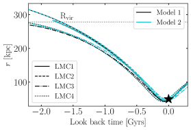
Figure 3: The separation of the LMC’s COM from that of the MW as a function of time from the $N$-body simulations. Results are illustrated for the four different LMC models using the isotropic (Model 1; black lines) and anisotropic (Model 2; blue lines) MW models. Note that the orbits are not arranged by mass. As such, the most massive LMC model does not reach the largest distance at infall (i.e. when its orbit crosses the virial radius of the MW). This is because the present-day position and velocity vectors are different in each simulation (see Appendix A), and the MW motion about the combined MW+LMC orbital barycenter increases with the mass of the LMC, impacting the inferred separation of the MW-LMC system at early times (Gómez et al., 2015). All orbits have pericenter distance and behavior consistent with backward analytic orbit integration using the observed proper motions (Salem et al., 2015). The black star shows the current position of the LMC. Even though there are small deviations between the orbits, all orbits are roughly consistent with each other over the last 1 Gyr. Therefore, the kinematics of the LMC’s orbit are not a significant variable in this analysis (Besla et al., 2007; Kallivayalil et al., 2013).

Sim.	LMC model	$\Delta r$ (kpc)	$\Delta v$ (km/s)	MW Model
$1$	LMC1	$2.51$	$49.05$	1
$2$	LMC2	$4.36$	$64.43$	1
$3$	LMC3	$2.49$	$26.77$	1
$4$	LMC4	$2.88$	$31.99$	1
$5$	LMC1	$1.83$	$53.39$	2
$6$	LMC2	$2.98$	$65.12$	2
$7$	LMC3	$2.29$	$44.89$	2
$8$	LMC4	$3.54$	$56.71$	2

Table 3: Summary of the simulations. $\Delta r$ and $\Delta v$ denote the difference in the magnitude of the simulated present-day LMC 3-D position and velocity vectors with respect to the observed values of (Kallivayalil et al., 2013). The MW kinematic profile is either isotropic ($\beta=0$; Model 1) or radially anisotropic ( $\beta(r)=-0.15-0.2\alpha(r)$; Model 2). The fiducial simulations are Sim. 3 and 7, marked in bold.

3.4 Constructing the MW’s Stellar Halo: Tagging DM Particles

In this study, we will track perturbations in the density and kinematics of the MW’s DM halo induced by the LMC and aim to relate them to observations of the MW’s stellar halo. However, the $N$-body models of the MW created in this study do not explicitly include a live stellar halo due to its negligible self-gravity. Instead, we build a mock smooth stellar halo using a weighting scheme implemented by Laporte et al. (2013a, b) (see also, Bullock & Johnston, 2005; Peñarrubia et al., 2008).

In short, the technique works as follows. We compute the fraction of stellar particles in energy bins, $N_{\star}(E)$, from the distribution function and the density of states of the DM particles of the MW’s halo (we do this separately for both Model 1 and Model 2). The ratio of $N_{\star}(E)$ to the fraction of DM particles in each energy bin, $N(E)$, provides the weight, $\omega$, that each DM particle contributes to a stellar halo particle within that energy bin. That is,

$$\omega(E)=\frac{N_{\star}(E)}{N(E)}=\frac{f(E_{\star})}{f(E)},$$ (4)

where the differential energy distribution is defined in terms of the density of states, $g(E)$, and the distribution function, $f_{\star}(E)$, as

$$N_{\star}(E)=g(E)f_{\star}(E).$$ (5)

To compute the kinematics of the stellar halo particles, we utilize weights $\omega$, for the DM particles, as follows:

$$\sigma=\frac{\sum_{i}\omega_{i}(v_{i}-\bar{v})}{\sum_{i}\omega_{i}},$$ (6)

where $v_{i}$ are the DM velocities of each particle, and $\bar{v}$ are the mean velocities of all of the DM particles. We assign the weights using the stabilized isolated MW models (i.e. after 2.5 Gyr of evolution in isolation; see § 3.2.1). Because the DM halo is spherical and in equilibrium, the distribution function of the DM halo can be computed using Eddington’s equation (Eddington, 1916). We build two stellar halos for each MW model: MW-X and MW-H. Both stellar halos have Einasto density profiles (Einasto, 1965),

$$\nu(r)=\nu_{e}e^{-dn(r/r_{eff})^{(1/n)-1}},$$ (7)

where $\nu_{e}$ is the normalization set by the total mass of the stellar halo. For our purposes, since we are measuring relative changes, the value of $\nu_{e}$ is set to 1. For values of $n$ larger than 0.5, $dn$ is defined as in Merritt et al. (2006):

$$dn=3n-1/3+0.0079/n.$$ (8)

The use of this profile is motivated by recent observations of K-Giants (MW-X; Xue et al., 2015) and RR Lyrae (MW-H; Hernitschek et al., 2018). See Table 4 for parameter details.

	MW-X	MW-H
Density profile	Einasto	Einasto
($n$; $r_{eff}$)	(3.1; 15 kpc)	(9.53; 1.07 kpc)
Distances (kpc)	10$-$80	20$-$131
Tracers	K-giants	RRLyr
Reference	Xue et al. (2015)	Hernitschek et al. (2018)

Table 4: MW stellar halo model parameters from observations of K-giants and RR Lyrae (RRLyr).

Figure 4 shows the resulting initial stellar halo number density (#/kpc³) and Figure 5 shows the velocity dispersion profiles (tangential, $\sigma_{t}$, and radial, $\sigma_{r}$) using this outlined technique for MW Models 1 and 2. The results for the initial isolated MW DM halos are also shown for comparison.

The MW-H density profile does not decrease as fast as MW-X with increasing Galactocentric radius. On the other hand, the velocity dispersion profile is flatter for MW-X. Note that in this analysis, we extrapolate the density and kinematic profiles of the stellar halo to distances larger than 100 kpc. This could be, in principle, an oversimplification since the outer halo likely is not smooth; however, it lets us understand the simplest scenario as a first step.

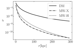
Figure 4: Initial number density profiles of the stellar halo (#/kpc³), built by applying the stellar tracer method, outlined in Laporte et al. (2013a, b), and using the observed density profiles for K-giants (MW-X; dashed line Xue et al., 2015) and RR Lyrae (Hernitschek et al., 2018, MW-H; dotted line). The DM density profile for the MW halo (solid line) is shown for comparison. This stellar halos are going to be used in both Models 1 and 2.

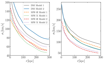
Figure 5: Radial ($\sigma_{r}$; left panel) and Tangential ($\sigma_{t}$; right panel) dispersion profiles corresponding to the stellar halo profiles from Figure 4 (colored lines). Results for the DM particles (solid lines) are shown for Model 1 (gray) and Model 2 (blue). Using this scheme, the dispersion profiles for the stellar halo are not modeled to be the same as that of the DM halo.

4 Results: The Response of the MW’s DM and Stellar Halo to the LMC

Octant #	Longitude $(^{\circ})$	Latitude$(^{\circ})$	$t_{LB}$ (Gyr Ago)
$1$	$[-180,-90]$	$[-90,0]$	0 - 0.12
$2$	$[-90,0]$	$[-90,0]$	0.12 - 0.22
$3$	$[0,90]$	$[-90,0]$	0.22 - 1.06
$4$	$[90,180]$	$[-90,0]$	$-$
$5$	$[-180,-90]$	$[0,90]$	$-$
$6$	$[-90,0]$	$[0,90]$	$-$
$7$	$[0,90]$	$[0,90]$	1.06 - 2.36
$8$	$[90,180]$	$[0,90]$	$-$

Table 5: Definition of the Octants illustrated in the Mollweide projection in Figure 6 in Galactocentric coordinates (Longitude and Latitude). The last column shows the look back time in Gyr, indicating the time since the LMC traveled through the given Octant. If no time is shown it is because the LMC never passed through that Octant. The LMC spends the majority of its recent orbital history traveling in Octants 7 & 3. It is currently located in Octants 1 & 2.

Here, we study the perturbations induced by the LMC in the properties of a smooth stellar halo (§ 3.4) that is in equilibrium with the MW’s DM halo, which is either initially isotropic (Model 1) or radially anisotropic (Model 2).

We aim to identify regions of the stellar halo that are responding to the passage of the LMC. Figure 6, shows the past and future orbit of the LMC in a Mollweide projection using Galactocentric coordinates following the convention of the Astropy library . The numbers in blue indicate Octants, which are defined in Table 5. The decomposition of the sky into Octants is used to guide the analysis, allowing us to relate the past location of the LMC to specific areas in the stellar halo. The LMC starts at the virial radius of the MW in Octant 7. The star illustrates the present-day position of the LMC (which is located in Octants 1 and 2). The future orbit of the LMC is depicted by the points to the left of the star, moving through Octants 1 and 5. The colorbar represents the Galactocentric distance of the LMC along its orbit. The LMC reaches Octant 5 at a distance of $\sim$120 kpc. It takes $\sim 2$ Gyr for the LMC to travel from $R_{vir}$ to its current location, which is marked by the red star.

In the following, we quantify the perturbations in the density (§4.1) and kinematics (§4.2) of the stellar halo induced by the LMC at three different Galactocentric radii: at 45 kpc, where the effects of the LMC on the halo are the strongest, and at 70 kpc, to illustrate the extent to which the LMC’s perturbations can be traced in the frontier discovery space for LSST and future surveys.

Note that we discuss only results for the fiducial LMC model of $\rm{M}_{vir}=1.8\times 10^{11}$ M_⊙ on the properties of the two different MW halo models (Sims 3 and 7 in Table 3). Later, we will discuss how our results change as a function of the LMC’s infall mass (§6.2).

Figure 6: Mollweide projection of the LMC’s orbit from the fiducial isotropic simulation (Sim. 3), with Galactocentric longitude and latitude values marked in degrees. We use the convention for Galactocentric coordinates as defined in the Astropy library. Numbers denote Octants on the sky, defined in Table 5, which are used as a reference for tracking the orbit of the LMC on the sky. The LMC enters the halo in Octant 7 ($\sim$ 2 Gyr ago) and is currently between Octants 1 and 2 (marked by the red star). It reaches pericenter in Octant 2, $\sim$50 Myr ago at a distance of $\sim$45 kpc. Octants 5 and 6 represent the predicted orbit of the LMC 0.5 Gyr into the future. The colorbar represents the Galactocentric distance of the LMC at each point in its orbit. The orbits from all LMC-MW simulations are very similar; see Figure 3. Note that this viewing perspective is flipped with respect to traditional Mollweide projections ($-180^{\circ}\leq$ lon $\leq 180^{\circ}$).

4.1 Density Perturbations Induced by the LMC: The LMC’s DM Wake

In this section, we study the density perturbations induced within the MW’s DM and stellar halo owing to the recent orbit of a massive LMC.

4.1.1 The DM Halo Wake in Cartesian Coordinates

Figure 7 illustrates the density perturbations ($\Delta\rho$) to the MW’s DM halo (Models 1 and 2) by the LMC in Cartesian coordinates. Changes in the local MW DM density are measured with respect to the MW’s halo in isolation (prior to the infall of the LMC; $MW_{iso}$). This is defined as:

$$\Delta\rho_{DM}=\frac{\rho_{MW}}{\rho_{MW_{iso}}}-1.$$ (9)

Note that LMC particles are not included in this calculation. Figure 7 shows a slice, 10 kpc in thickness, of the present-day simulated MW DM halo in the Galactocentric $y-z$ plane, which is roughly co-planar with the LMC’s orbital plane. The MW’s disk lies in the $x-y$ plane, and the Sun is located at $x=-8.3$ kpc.

Figure 7 reveals the extended and anisotropic nature of the DM halo wake. We identify three main components:

1. A Transient response, seen as a DM overdensity trailing the LMC along its orbit. This feature is marked by solid contours (red regions at positive $y$). This is analogous to the classical Chandrasekhar wake.

2. A large underdense region shown with dashed contours (blue regions) south of the Transient response. We call this the Global Underdensity.

3. An extended overdensity in the Galactic north, shown with solid black contours (red regions at positive $z$ and negative $y$). This Collective response covers roughly one quarter of the sky.

These maps indicate that the perturbations in the density field of the MW’s DM halo are stronger at larger Galactocentric distances, $R_{GC}>45$ kpc. This likely reflects the longer duration that the LMC spend in those regions. Within 45 kpc, the halo wake is the weakest since the LMC has not yet passed through the inner halo. Yet, the LMC does impact the structure of the MW’s outer disk (Laporte et al., 2018a). According to Weinberg (1989, 1995, 1998b); Choi et al. (2009), an inner DM wake should also be created due to inner resonances, but this is not apparent in these simulations, likely due to the LMC’s high speed. The resonant modes induced in the halo will be quantified in upcoming work (Garavito-Camargo et al in prep).

Overall, the density maps agree for both Models 1 and 2. However, we note some differences: 1) the Transient response is stronger in Model 2 (left panel in Figure 7); 2) the Collective response is stronger for Model 1; 3) the morphology of the Transient and Collective DM responses, and the Global Underdensity vary slightly. These differences are a consequence of the internal kinematics of the two DM halo models as also found by Amorisco in prep.

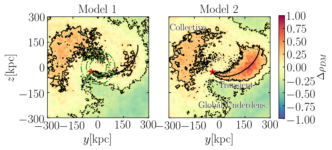
Figure 7: Density perturbations, revealing the DM halo wake induced by the LMC in the MW’s DM halo in the $y-z$ Galactocentric plane, which is almost coplanar with the LMC’s orbit. The MW’s disk is in the $x-y$ plane, where the Sun is located at $x=-8.3$ kpc. Results are for a slice, 10 kpc in thickness, centered at $x=0$. The green circles illustrate galactocentric distances of 45, 70 and 100 kpc. No LMC particles are included in this plot. The color map illustrates the density ratio of the MW’s DM distribution at the present day with respect to that of the MW in isolation (prior to the infall of the LMC) for Model 1 (left) and Model 2 (right). Red colors indicate overdense regions and blue underdense regions. The current position of the LMC is represented by a red star and its orbital path is traced by the solid black line. Contours indicate underdensities of $\Delta\rho_{DM}=$ 0.8 (dashed) and overdensities of $\Delta\rho_{DM}=$1.2 (solid). Three main morphological features are identified. 1) The Transient response: the DM overdensity trailing the LMC, tracing its past orbit. 2) The Collective response: An overdensity that appears in the north (at $z>0$ & $y<0$). 3) The Global Underdensity: Underdense regions that surround the Transient response. The morphology and the strength of these features are somewhat different for both the isotropic (Model 1; left panel) and anisotropic (Model2; right panel) MW halos, reflecting the resonant nature of the DM halo. In particular, the overdensity in the DM wake is stronger in Model 2.

4.1.2 The Wake in the Stellar Halo: Mollweide Projections.

In this section, we explore how the DM wake induced by the LMC manifests within the stellar halo. In Figure 8, we use the methodology outlined in §3.4 to identify the corresponding density perturbations seen in Figure 7 in a Mollweide map of the MW’s stellar halo.

The density perturbations are computed as follows. We build a grid, with cell size of projected area $(1.6^{\circ})^{2}$, on a spherical shell, 5 kpc in thickness, at a given Galactocentric radius. We define grid points as the corners of each cell. At each grid point, we compute the local density, $\rho(r)$, using the 1000 nearest particles. At 200 kpc, the outskirts of the halo, grid cells correspond to a volume of a cell of 13 kpc length and 5 kpc thickness.

The color scale in Figure 8 represents $\Delta\rho$, which we define as the ratio between the local stellar density, $\rho(r)$, and the mean stellar density across the all-sky spherical shell, $\overline{\rho(r)}$:

$$\Delta\rho(r)=\frac{\rho(r)}{\overline{\rho(r)}}-1.$$ (10)

Results are shown for spherical shells at 45, 70, and 100 kpc, centered on the Galactic center (see https://bit.ly/2S25YzC for additional plots at distances of 25, 150, and 200 kpc).

Given that the stellar halo is modeled in equilibrium with the DM halo, the same three features of the DM halo wake seen in Figure 7 are also apparent in Figure 8. Furthermore, using the Mollweide projection, we can now identify the locations of these features on the sky.

1. The Transient response. In the south, there exists a local stellar overdensity, coincident with the Transient DM wake, tracing the past orbit of the LMC (red region tracked by open black stars). The stellar Transient response persists over distances from 45 to 100 kpc (Figure 8) and even at distances as large as 200 kpc.

2. The Collective response. An extended overdensity is apparent in the north, between Octants 5 and 8, at all distances. This coincides with the Collective DM response that is generated by both resonances and the displacement of the orbital barycenter.

3. The Global Underdensity. In the south, primarily on either side of the Transient response, underdense regions (blue) are apparent, reflecting the removal of stellar mass and DM from these regions to form the higher-density Transient and Global responses.

Perturbations in the stellar halo at distances smaller than 45 kpc do exist, but the amplitude is significantly lower. Instead, we focus our analysis on the strongest wake amplitude in the hopes of devising a viable observational strategy (see §5.1) to capture signatures of the wake in the stellar halo.

We again see differences between the density perturbations in Model 1 vs. Model 2, indicating that the internal kinematics of the DM halo affect the morphology and amplitude of the wake within the stellar halo. The dashed and solid contours are at the same density enhancement in both models, illustrating that the wake is consistently stronger in Model 2. Regardless of the detailed internal kinematics of the DM halo, we find that perturbations to the stellar halo caused by the LMC persist for 2 Gyr and will cover a very large volume of the stellar halo.

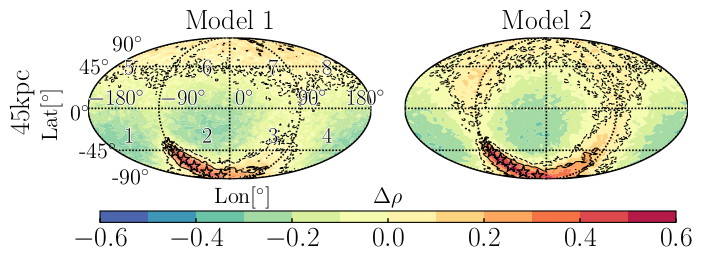
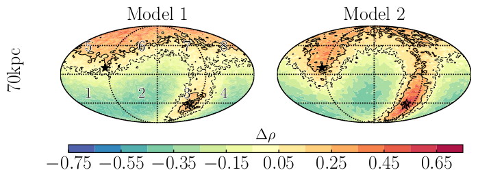
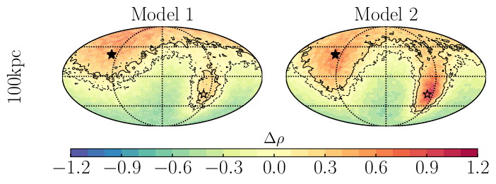
Figure 8: Mollweide maps of the MW stellar halo, illustrating local enhancements and decrements in stellar density within a spherical shell, 5 kpc in thickness, at three illustrative Galactocentric radii: 45 kpc (top), 70 kpc (middle), and 100 kpc (bottom). Results are shown for the MW-X halo that follows the K-giant density profile of Xue et al. (2015) constructed in equilibrium with the the MW halo Model 1 (isotropic; left panel) and Model 2 (anisotropic; right panel); results are similar for the MW-H model. The color bar represents the ratio between the local density at a given grid point, $\rho(r)_{local}$, with respect to the spherical average in the shell at that distance, $\overline{\rho(r)}$. The open black stars represent the past orbital path of the LMC at each Galactocentric distance, while the solid black stars indicate its future orbit. Contours mark stellar overdensities of $\Delta\rho=$0.1 (dashed) and $\Delta\rho=$0.2 (solid) relative to the mean in all panels except at 100 kpc, where contours mark overdensities of $\Delta\rho=$0.2 (dashed) and $\Delta\rho=$0.6 (solid). The stellar halo exhibits a stellar wake that tracks that of the DM halo and is similarly composed of three main features: (1) the Transient response tracing the LMC’s past orbit in the south (red region marked by open stars); (2) the Collective response, seen as a large red overdensity in the north that persists at all distances; and (3) the Global Underdensity, seen as blue regions surrounding the stellar Transient response in the south. The contours illustrate that the initial halo kinematics impact the amplitude of the Transient response, which is more pronounced in Model 2 than Model 1. The Collective response is very extended and its structure and amplitude depend only mildly on the initial kinematic structure of the halo.

4.2 Kinematic Perturbations in the Stellar Halo: The Kinematics of the LMC’s Wake

As seen in the previous section, the DM and stellar halos are perturbed by the passage of the LMC, resulting in regions of over- and underdensities. This requires the displacement of mass in the halo (e.g. Buschmann et al., 2018). Here, we identify the kinematic signatures of this motion. These signatures complement the density perturbations studied in the previous section and provide key observables for the identification of the wake.

We compute the local mean velocities and velocity dispersions of the stellar halo using the nearest 1000 particles at each grid point in the Mollweide projections, as in Figure 8.

All kinematic quantities are computed in Galactocentric coordinates. As in the previous section, we present results at three illustrative Galactocentric distances: 45, 70 and 100 (for $\Delta\sigma_{r}$) kpc (in https://bit.ly/2S25YzC we include the corresponding plots at 25, 100, 150 and 200 kpc). We first show our results for the radial velocities (§4.2.1), followed by the tangential motion (§4.2.2).

4.2.1 Radial Motions in the Stellar Halo.

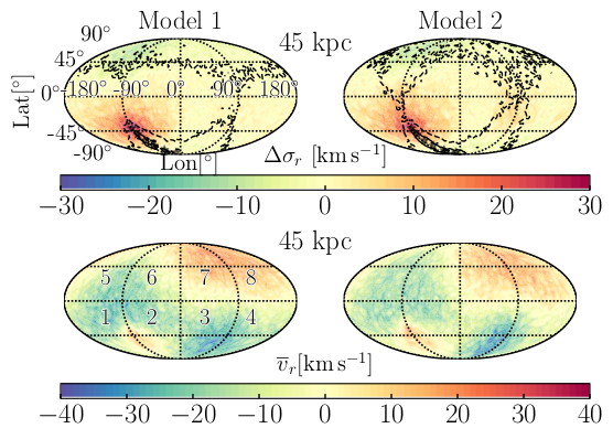
Figure 9: Mollweide projection in Galactocentric coordinates illustrating radial motions of the stellar halo. The top panel shows the radial-velocity dispersion relative to the average computed over a spherical shell, 5 kpc in thickness, at 45 kpc, $\Delta\sigma_{r}=\sigma_{r}/\overline{\sigma_{r}}$. The bottom panel illustrates the local mean radial velocities, $\overline{v_{r}}$, across the same spherical shell. Results are similar for both Model 1 (left) and Model 2 (right). Contours illustrate the location of overdensities in the north (Collective response) and the south (Transient response), representing density enhancements, $\Delta\rho$, of 0.0 and 0.4 relative to the mean density (see Figure 8). The gray stars show the past orbit of the LMC at this distance. Local values of both $\sigma_{r}$ and $\overline{v_{r}}$ are measured using the 1000 nearest stellar particles within a grid cell of $1.6^{\circ}$ squared. For the top panels, the color scale indicates increases (red) or decreases (blue) in $\sigma(r)$ relative to the shell average. In the bottom panels the color bar indicates the direction of average radial motions, $\overline{v_{r}}$, on the sky (blueshift or redshift). $\sigma_{r}$ increases by $\sim$25 km/s near the LMC (Octants 1 and 2), leading the Transient response, and decreases by $\sim$14 km/s to the north of the LMC (Octants 4 and 5), forming a kinematically “cold region”. The latter coincides with the Collective response and the future orbital trajectory of the LMC. In contrast, the velocity dispersion in Octants 7 and 8 in the north is largely unaffected. The radial motions, $\overline{v_{r}}$, illustrate that the region of the Transient response closest to the LMC (Octant 2) is moving away from the galactic center (redshifted; as is the LMC COM motion), but the Transient response further away from the LMC (Octants 3 and 4) follows the past orbital motion of the LMC toward the MW (blueshifted). On average, the northern Sky appears to be currently moving away from us.

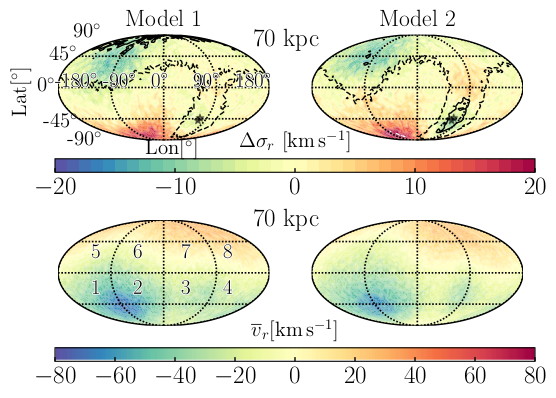
Figure 10: Same as Figure 9 but at 70 kpc. The gray tars mark the past location of the LMC on the stellar halo at this distance. The decrease in $\sigma_{r}$ still persists in the north (Octants 4 and 5) and appears more clearly associated with the Collective response. The increase in $\sigma_{r}$ in the south has moved, with respect to the 45 kpc case, on the stellar halo to reflect the past motion of the LMC, but still leads the Transient response. The mean radial velocities in the north indicate that the Collective response is still moving away from the MW disk, but now there is a comparably blueshifted region in the southern sky, forming a dipole pattern that may reflect the COM motion of the disk about the LMC-MW orbital barycenter.

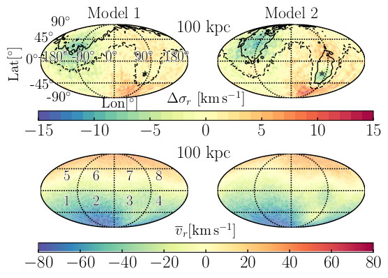
Figure 11: Same as Figure 9 but at 100 kpc. Results are similar to that of Figure 10, but the dipole pattern in the $\overline{v_{r}}$ is even more pronounced and the effect is very similar in both Model 1 and 2. This supports the idea that this velocity pattern is generated from the motion of the MW disk about a new orbital barycenter, as we expect the halo outskirts to exhibit the largest offsets with respect to the motion of the halo cusp.

Radial velocities are computed with respect to the Galactic center. Figures 9,10, and 11 show the change in the local radial Galactocentric velocity dispersion ($\sigma_{r}$) relative to the all-sky average dispersion ($\overline{\sigma_{r}}$):

$$\Delta\sigma_{r}(r)=\sigma_{r}-\overline{\sigma_{r}}$$ (11)

and the local mean radial velocity, $\overline{v_{r}}$ of the stellar halo at 45, 70, and 100 kpc, respectively. Again, local quantities are computed at each grid point, as in Figure 8.

At 45 kpc, the radial-velocity dispersion maps show two main features: (1) an increase in $\sigma_{r}$ of $\sim 25$ km/s near the LMC (Octants 1 and 2); and (2) a decrease in $\sigma_{r}$ by $\sim 14$ km/s, forming a “cold region”, in the north (Octant 5) that coincides with both the Collective response and the future of the orbit of the LMC. In the northern Octants 7 and 8, $\sigma_{r}$ appears unaffected by the LMC.

The increase in $\sigma_{r}$ in Octants 1 and 2 correlates with positive motions in $\overline{v_{r}}$ of $20$ km/s in the same region. The stars in the region of the Transient response closest to the LMC are thus tracing the COM motion the LMC, which is currently moving away from us (redshift). Further away from the LMC, stars in the Transient response trace the past orbital motion of the LMC toward the MW.

These kinematic perturbations persist at larger Galactocentric distances. In particular, the ‘cold region’ associated with the Collective response is more apparent at 70 kpc (Figure 10). Also, $\overline{v_{r}}$ is consistently negative (blueshifted) along the Transient response, following the orbit of the LMC (black stars) to large distances. There is thus a strong spatial correlation between $\overline{v_{r}}$ and the Transient response.

Overall, the results are consistent for Models 1 and 2, but the amplitude of the blueshift in $\overline{v_{r}}$ within the Transient response is larger in Model 2. This likely explains the increased strength of the Transient response in Model 2, seen in Figure 8. The kinematic profile of the halo in Model 2 is radially anisotropic, naturally boosting the Transient response signature, which follows the radially infalling orbit of the LMC.

The Collective response in the northern sky exhibits positive radial velocities, indicating that this region is moving away from the MW’s disk. Moreover, at larger distances (Figures 10 and 11), radial motions increase, approaching the COM motion of the MW’s disk ($\sim$56 km/s in Sim. 3). In the south, we see negative radial velocities, particularly in Octants 1 and 2. Furthermore, the velocity pattern at 100 kpc is very similar in both Model 1 and Model 2. Together, these results support the idea that this pattern results from the motion of the MW’s disk about the new LMC-MW orbital barycenter. The disk is moving toward the location of the LMC at its pericentric approach (Octant 3) and so the radial-velocity pattern seen in the outer halo is thus the reflex of this motion: the northern sky displays redshifted motions and the south blueshifts.

4.2.2 Tangential Motions in the Stellar Halo

We compute the tangential motions of the stellar halo particles with respect to the Galactic center. We consider the tangential motions of stars in the stellar halo separately in both the latitudinal ($Lat$) and longitudinal components ($Lon$) in Galactocentric coordinates.

Latitudinal Motions:

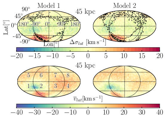
Figure 12: Mollweide projection in Galactocentric coordinates illustrating the ratio of the local latitudinal tangential velocity dispersion with respect to the all-sky average ($\Delta\sigma_{lat}$; top panels) and the local mean latitudinal tangential velocity ($\overline{v_{lat}}$; bottom panels). $\sigma_{lat}$ increases by 20 km/s within the Transient response in Octants 1 and 2. For $\overline{v_{lat}}$, the color scale also indicates the direction of motion in latitude (positive is toward the north and negative is toward the south). north of the the LMC, between $-45<Lat<0$, $\sigma_{lat}$ decreases by $\sim 10$ km/s and increases up to $20$ km/s between $-90<Lat<-45$; the latter traces the Transient response. This bipolar behavior in $\overline{v_{Lat}}$ illustrates that stars both north and south of the LMC are being gravitationally pulled toward the LMC.

Figures 12 and 13 illustrate the change of the local latitudinal tangential velocity dispersion with respect to to the all-sky average:

$$\Delta\sigma_{lat}=\sigma_{lat}-\overline{\sigma_{lat}}$$ (12)

and the mean local latitudinal tangential velocity ($\overline{v}_{lat}$) of stars in the stellar halo at 45 and 70 kpc, respectively.

At 45 kpc, Octants 1 and 2 show the strongest changes in $\sigma_{lat}$, increasing by 20 km/s in the Transient response. $\overline{v_{lat}}$ exhibits a bipolar behavior north and south of the LMC, indicating that stars are being gravitationally focused toward the LMC’s COM.

At larger distances, Figures 13 illustrate that an increase in $\sigma_{lat}$ consistently leads to the Transient response. The behavior of $\overline{v_{lat}}$ shows more complex patterns at distances beyond 45 kpc. However, the kinematics still illustrate motion along the Transient response (negative values, indicating motion toward the south in Octants 3 and 4). We find this behavior at the outer regions of the halo too, but here we just show the results at 70 kpc for illustrative purposes.

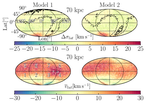
Figure 13: Same as Figure 12 but at 70 kpc. An increase in $\sigma_{lat}$ leads to the Transient response. The behavior of $\overline{v_{lat}}$ is more complex, but there is still evidence for negative motions along the Transient response (following the LMC’s orbit).

Longitudinal Motions:

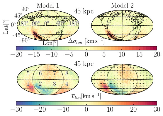
Figure 14: Same as Figure 12 except for the tangential motion in Galactocentric longitude. The color bar indicates the magnitude of local changes in the dispersion, $\sigma_{lon}$, relative to the all-sky average and both the magnitude and the direction of the local mean velocity, $\overline{v_{lon}}$, where negative indicates toward more negative longitudes and positive toward more positive longitudes (see arrows on the bottom right panel for guidance). $\sigma_{lon}$ increases at the location of the LMC by $\sim 20$ km/s. Surrounding the LMC, the direction of $\overline{v_{lon}}$ indicates a corresponding converging flow of particles moving toward the LMC. Further along the Transient response, the flow of stars is diverging (Octants 3 and 4). This flow results from the motions of stars that were once converging toward the LMC as it passed through that location of the sky.

Figures 14 and  15 illustrate the ratio of the local stellar longitudinal tangential velocity dispersion with respect to the shell average:

$$\Delta\sigma_{lon}=\sigma_{lon}-\overline{\sigma_{lon}}$$ (13)

and the local mean longitudinal tangential velocity ($\overline{v}_{lon}$) at 45 and 70 kpc, respectively.

At 45 kpc, the velocity dispersion, $\sigma_{lon}$, increases by $\sim 20$ km/s in the vicinity of the LMC. Surrounding the LMC, $\overline{v_{lon}}$ indicates motions converging toward the LMC. Together with Figure 12 and Figure 14, these results indicate that the motions of particles in the vicinity of the LMC are being gravitationally attracted to it.

At 70 kpc, Figures 15 illustrates kinematics directly related to the motion of particles in and surrounding the Transient response.

On the other hand, in Octants 3 and 4, there is a divergent flow of stars in extended regions around $l=90^{\circ}$ in $\sigma_{lon}$. This flow is the result of stars that were converging toward the LMC when it passed through that location of the sky $\sim 0.4$ Gyr ago, corresponding to the formation of the Transient response at that time. At the present day, those converging stars continued in their motion through the Transient response, and now appear to be diverging. The $\overline{v_{lon}}$ maps reveal that particles in those regions are moving with opposite directions in longitudes, again exhibiting diverging motions. The Transient response is located between these two regions, where the velocity dispersion is lower. The kinematic imprint of the Transient response beyond 45 kpc is thus stronger in the longitudinal component than in either the latitudinal or the radial-velocity components. We find this effect to increase at distances larger than 70 kpc.

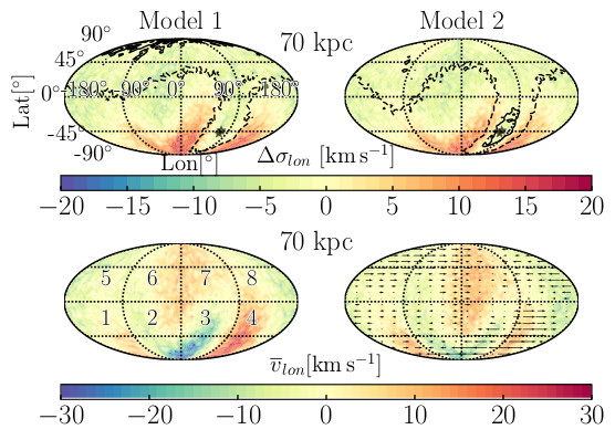
Figure 15: Same as Figure 14 but at 70 kpc. $\sigma_{lon}$ increases by $\sim$20 km/s surrounding the stellar wake. This has a corresponding signature in $\overline{v_{lon}}$ as diverging motions, moving away from the Transient response. This is in contrast to the results in the latitudinal tangential component, where motions appeared to follow the direction of the LMC orbit Transient response (Figure 12).

4.2.3 Assessment of the Kinematic State of the Halo

Our results indicate that the MW’s stellar halo should hold kinematic signatures of the Transient and Collective responses induced by the passage of the LMC. These effects manifest themselves as global, correlated kinematic patterns across the sky that persist over large ranges of Galactocentric distances, making them distinct from thin substructures that are characteristic of disrupting satellites or globular clusters.

The Transient response is most apparent kinematically in the tangential motions of the stellar halo, resulting in anticorrelated responses in Galactocentric longitudes and latitudes. Specifically, the velocity dispersion in $\sigma_{lat}$ increases in the Transient response itself whereas $\sigma_{lon}$ increases in the regions surrounding the Transient response.

In contrast, the Collective response is best tracked by radial velocities, which likely reflects the reflex motion of the MW’s disk about the orbital barycenter of the LMC-MW system, resulting in global redshifts in the north, vs. blueshifts in the south.

Overall, the impact on the MW’s stellar halo kinematics across the sky in the tangential component is very similar for both Models 1 and 2, although the amplitude of the perturbation is typically stronger in Model 2. Given that these two MW models have very different kinematics, we conclude that our conclusions are robust to any initial anisotropy in the kinematic structure of the halo.

Furthermore, the measured increase in both the radial and tangential velocity dispersions by as much as 20-30 km/s, suggests that the stellar halo is being ‘heated’ and is not in equilibrium locally.

We compute the change in the anisotropy parameter as the difference between the local anisotropy parameter, computed over the nearest 1000 neighbors within a grid cell ($\Delta\beta$), relative to the all-sky average ($\overline{\beta}$):

$$\Delta\beta=\beta-\overline{\beta}.$$ (14)

The resulting all-sky map of $\Delta\beta$ for the simulated stellar halo in Sim. 7 (Model 2) within a spherical shell (5 kpc in thickness) at a Galactocentric distance of 45 kpc is shown in Figure 16. Versions of this map are also created for Model 1 and for shells at different distances in both models, see https://bit.ly/2S25Yz. We find that $\beta$ varies over large regions of the sky and distances. The largest positive values of $\beta$ (as high as 0.3) are induced at 45 kpc, as shown in Figure 16.

The Collective response in the north, which exhibited a ‘cold spot’ region in the radial-velocity dispersion (Figure 9), corresponds to a decrease in $\beta$ of -0.25. This structure persists out to the virial radius. Decreases in $\beta$ are also seen corresponding to the Transient response at distances greater than 70 kpc. This corresponds to changes in the tangential velocity dispersion, which are discussed in $\S$ 4.2.2.

Recently, Cunningham et al. (2019) studied the impact of substructure on $\beta$ using two of the Latte FIRE-2 (Wetzel et al., 2016) cosmological simulations. The stellar particles from substructures in the MW halo have different kinematics than the stellar halo and thus produce local changes in $\beta$ from -1 to 1. Note that these substructures are smaller than the LMC and are not perturbing the stellar halo itself. However, distinguishing between small substructures and the perturbations on the stellar halo due to the LMC could potentially be done using $\beta$. Thus, compared to our results, we note that the effect of the LMC, without including the LMC stellar particles, on $\beta$ is $\sim$ 20% (30% for the isotropic MW models) of that from substructure. In addition, the LMC should perturb some of the substructure in the stellar halo e.g., Erkal et al. (2019). Future work examining this scenario in a cosmological setting, i.e. including both the LMC and substructure, will be done to properly capture the global perturbations in $\beta$. In the mean time, the results presented in Figure 16 show that the effect of the LMC on $\beta$ is not negligible when compared to perturbations expected from local substructure.

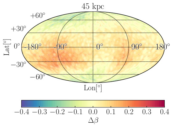
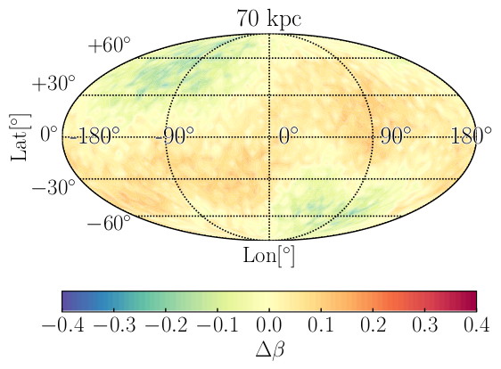
Figure 16: Mollweide plots of the difference in the local value of the anisotropy parameter relative to the average ($\Delta\beta$, Equation 14) computed within a spherical shell, 5 kpc in thickness at 45 (top) and 70 (bottom) kpc using Sim. 7 (Model 2). $\Delta\beta$ ranges from -0.25 to 0.25. Increases in $\beta$ are found preferentially near the plane of the MW while decreases are found toward the poles of the MW. Results at different distances and for Model 1 can be found here http://jngaravitoc.github.io/Garavito-Camargo/research/lmc_wake/. These results suggest that the LMC has a nonnegligible effect on $\beta$. At 70 kpc, the effects of both the Transient and Collective response can be seen as decreases in $\beta$.

5 Observability of the Wake

In the previous sections, we characterized the density and the kinematic imprint of the interaction between the MW and the LMC in the stellar halo. In this section, we assess the observability of our results, including observational errors in both distances, and velocities. We also select regions of the sky within current or upcoming survey footprints to outline example observing strategies.

We start our analysis by exploring the observability of the density enhancements in the Transient and Collective responses induced by the LMC (§5.1). In §5.2, we focus on the kinematic signature of these structures in the angular and radial components of the velocity dispersion.

Finally, we estimate the number of particles/stars needed in order to measure the predicted perturbations (§5.3).

The aim of this section is to provide the reader with a sense of how to sample the global patterns induced by the passage of the LMC on the smooth component of the stellar halo, rather than to make concrete predictions for specific surveys. A standing problem to observe these global patterns is the presence of substructure in the stellar halo (e.g., Bullock & Johnston, 2005). Distinguishing substructure from the global patterns of the LMC wake might be possible by using combinations of the predicted signatures in both density and kinematics. We anticipate that the global patterns corresponding to the Transient and Collective responses should be present in the halo despite substructure and will persist over significantly larger distances than expected for tidal streams or individual satellites.

Region	Quantity	Longitude $[^{\circ}]$	Latitude $[^{\circ}]$
Regions 1-7	$\sigma_{r}$	[-129, -122, -118, -118, -100, -100, -100, -90, -90]	[67, 67, 66, 60, 55, 55, 50, 45, 45]
Region 8	$\sigma_{r}$	45	45
Region 9	$\sigma_{lon,lat}$	130	-55
Region 10	$\sigma_{lon,lat}$	80	-45
Regions 11-14	$\rho_{\textit{transient}}$ overdensities	[-90, 90, 80, 90]	[-45, -45, -25, 15]
Region 15	$\rho_{\textit{transient}}$ underdensities	145	-50
Region 16	$\rho_{\textit{collective}}$ overdensities	-90	45
Region 17	$\rho_{\textit{collective}}$ underdensities	145	-50

Table 6: Galactocentric coordinates of the centers of the target regions of the sky for the proposed observations. The regions are $20^{\circ}$ in width in both longitude and latitude. Regions 1-7 have coordinates centers that correspond to distances of [20, 30, 40, 50, 60, 70, 80, 90, 100] kpc respectively. For regions 8-10 the same coordinates centers are used at all the distances. Regions 11-14 have coordinate centers that correspond to distances of [45, 70, 100, 200] kpc respectively, whereas Regions 15-17 have the same coordinates centers at every distance (see Figure 19). Transient and Collective refers to regions assigned to observe the Transient and Collective responses respectively.

5.1 Observing Density Enhancements Associated with the Transient and Collective responses

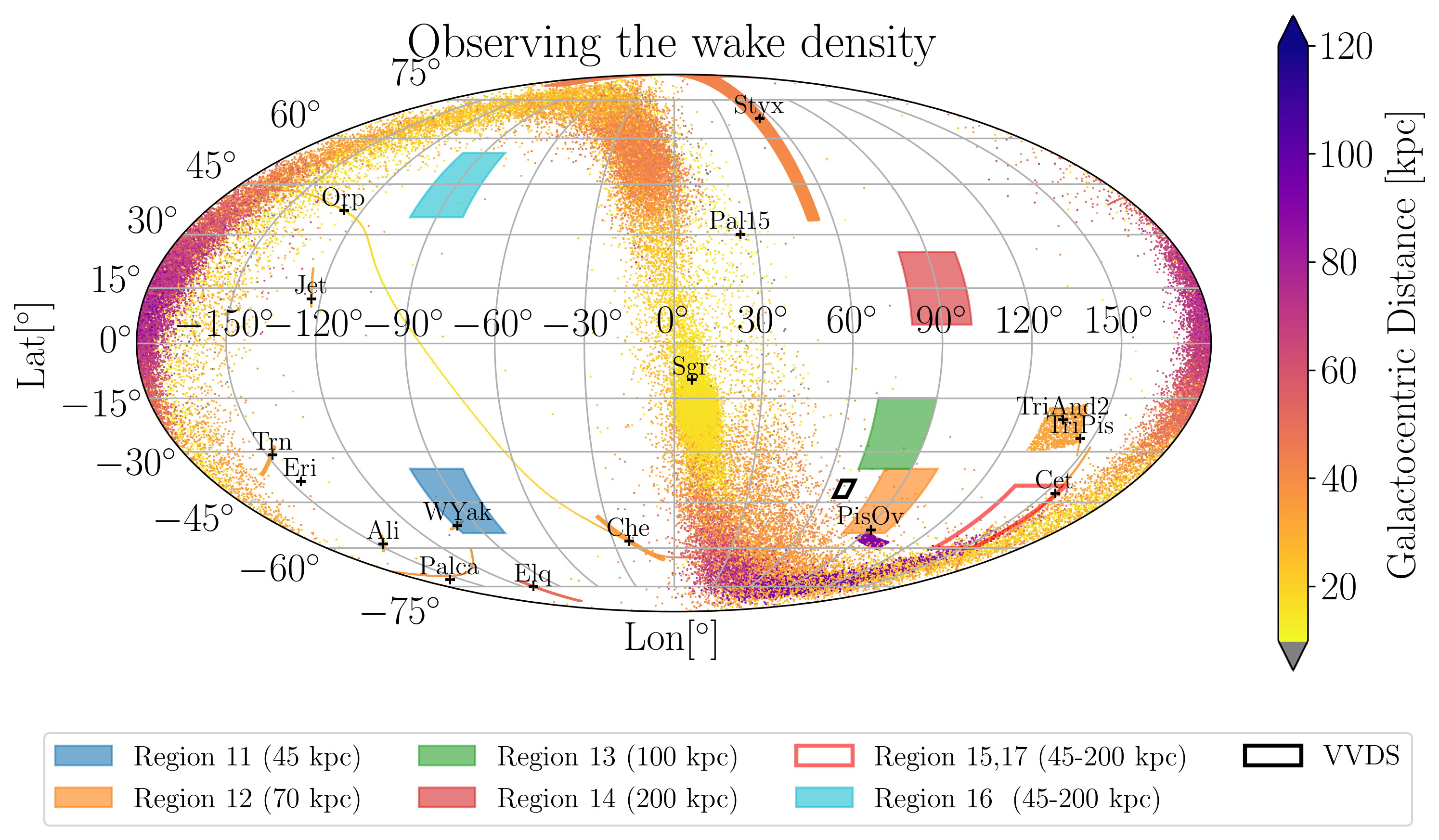
Figure 17: Observing strategies for identifying the wake using stellar densities: illustration of observing strategies to identify the predicted Transient and Collective responses induced by the LMC within the stellar halo. The figure shows a Mollweide projection in Galactocentric coordinates marking the location of the currently known stellar streams that extend or are at distances greater than 50 kpc. The color bar indicates the Galactocentric distance of the streams. The most prominent substructure is the stellar stream from the Sag dSph. Also marked is the location of the VVDS survey (Deason et al., 2018) with a black empty square. We select regions in which less substructure is present, marked by colored squares, in order to illustrate the observability of the wake. Filled boxes indicate overdense regions tracking the Transient response (blue, orange, green, and red) and Collective response (cyan) at different Galactocentric radii. The empty red box marks an example of an underdense region that will be used compute the density contrast. The image was made using the GALSTREAMS library (Mateu et al., 2018).

Here, we study the observability of stellar density enhancements corresponding to the Transient and Collective responses induced by the LMC in the stellar halo. Our proposed strategy consists of measuring density ratios across the stellar halo, focusing on regions with few known substructures and where the relative change in density is predicted to be largest. We illustrate this strategy in Figure 17, which shows a map of the current known stellar streams beyond 30 kpc in a Mollweide projection in Galactocentric coordinates. The most prominent stream is that of the Sgr. dSph. We pick eight regions of 20 square degree at distances of 50, 70, 100, and 200 kpc that avoid the Sgr stream (see Table 6 for exact coordinates of the proposed regions). The cyan box indicates the overdensity on the Collective response. The blue, orange, green, and red boxes indicate regions centered on overdensities induced by the Transient response. The green box is centered on a region within the Collective response underdensity that will be used to compute the density contrast with the overdense regions. Note that there are multiple regions that could be chosen; here, we pick example regions that will be within the LSST footprint.

The results of this observing strategy to hunt for the Transient and Collective responses are shown in Figure 18. The average number density of stars located in the overdense regions ($\rho_{O}$) is divided by the average number density of stars in the underdense region ($\rho_{U}$). The resulting ratios are plotted as a function of the number of stars sampled inside the volume (a box of 20 square degrees and a thickness of 5 kpc).

In all cases, we have included assumed distance errors of 10% which account for the observational errors for typical current surveys. Furthermore, to account for observations being transformed to a Galactocentric frame, we also include a distance error of 0.09 kpc for the Sun’s Galactocentric position (McMillan, 2017). The error bars are computed using the bootstrapping technique and increase as the number of particles in each box decrease.

We find that the predicted density contrast is unaffected by the number of particles used or by the distance errors. These results suggest that measurements of 20-30 stars within each volume are sufficient to identify the Transient and Collective responses. Table 7 summarizes the corresponding number densities of stars within the selected regions (listed in Table 6) at different distances. In §5.3, we discuss our sampling relative to realistic expectations for the number density of stars at these distances.

$r$ (kpc)	$\nu$ [# of stars kpc-3]
45 kpc	$6.2\times 10^{-3}$ $\pm$ $1\times 10^{-4}$
70 kpc	$3.6\times 10^{-3}$ $\pm$ $2\times 10^{-4}$
100 kpc	$1.6\times 10^{-3}$ $\pm$ $1\times 10^{-4}$
200 kpc	$4\times 10^{-4}$ $\pm$ $5\times 10^{-5}$

Table 7: Stellar number densities ($\nu$) corresponding to 20 stars in a 20 square degree region of 5 kpc thickness (i.e. boxes in Figure 17 and 19) at the listed Galactocentric radius ($r$). This is the minimum density needed to observe the Transient and Collective responses as stellar overdensities.

Interestingly, Deason et al. (2018) recently reported the discovery of an extended overdensity of 17 stars along the orbit of the LMC at distances of 50-100 kpc (disappearing at smaller radii). The region is marked as VVDS in Figure 17. The authors attributed this material to stellar debris associated with Magellanic Stream. However, the spatial coincidence of these observations with expectations for the general location of the LMC’s Transient response are suggestive (see $\S$ 6.4). It is possible that other existing surveys may already have data to identify these proposed structures. We caution, however, that confirmation of the association of such overdensities with the LMC Transient and Collective responses must also involve matches with kinematic predictions, as outlined in §4.2 and discussed in the next section.

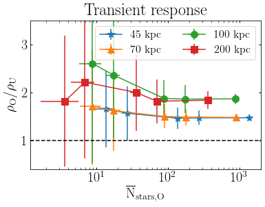
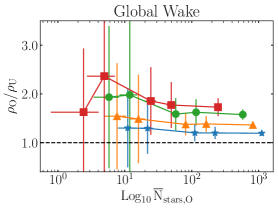
Figure 18: Observability of overdensities associated with the Transient and Collective responses as a function of the number of sampled DM particles (see table  6 for details). To study how our results we change as a function of number of stars, we randomly sample the DM halo with [$5,10,50,100,500$] $\times 10^{4}$ DM particles. With each of those samples, we proceed to measure the densities in the Regions 11 and 15 for the Transient response and 16 and 17 for the Collective response (see Table 6 for the coordinates of the proposed regions). Plotted are density ratios between overdense (O) and underdense (U) regions (marked in Figure 17) at different Galactocentric distances, including distance errors of 10% and an assumed uncertainty in the Sun’s Galactocentric distance of $\pm$0.09 kpc. Ratios are plotted as a function of the number of particles sampled in each overdense region ($N_{\rm part,O}$). The coordinates of the center of the O and U regions chosen for this experiment are listed in Table 6. Each region comprises a volume of $20$ square degree and 5 kpc in thickness. The errors in the distances and the number of particles used do not have a strong effect on the density ratio. The strength of both the Transient and Collective responses is stronger at larger distances, as discussed in § 4. We conclude that the Transient response induced by the LMC should be measurable even if there are only 20 stars in each 20 degree squared region. The corresponding minimum number density needed at each distance is listed in Table 7. See Figure 21 for an assessment of our choice of sampling of stars in the stellar halo.

5.2 Observing the Kinematic Signature of the LMC’s Wake

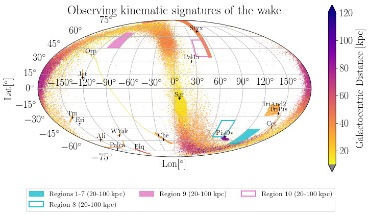
Figure 19: Observing strategies for kinematic signatures: same as Figure 17 but illustrating observing strategies designed to detect the kinematic signatures of the Transient and Collective responses due to the passage of the LMC in the stellar halo. Each colored square shows the regions in which a given component of the velocity dispersion is measured: $\sigma_{r}$ (magenta box; Collective response); $\sigma_{lat}$ and $\sigma_{lon}$ (cyan box; Transient response). Since we focus on relative changes in the velocity dispersion, each component is measured in two distinct regions, selected to both maximize the difference in the velocity dispersion and avoid known substructures. The empty and solid cyan boxes are adjacent to the density enhancement along the Transient response, which illustrates strong increases in $\sigma_{lon}$ (Figure 15) The solid magenta box is coincident with the ‘cold region’ of lower radial-velocity dispersion in the Collective response whereas the empty box is a relatively unperturbed region of the halo (Figure 10). For illustrative purposes, the test regions are selected within the DESI (for $\sigma_{r}$) and LSST (for $\sigma_{lat}$, $\sigma_{lon}$) footprints.

We discuss the observability of the kinematic signatures associated with the Transient and Collective responses induced in the stellar halo owing to the LMC’s passage, as studied in §4.2. We select example regions where the MW’s stellar halo is predicted to have the strongest kinematic response and that also avoid known substructures, as illustrated in Figure 19. We select the marked regions to measure the relative change in the average radial-velocity dispersion (tracing the Collective response) and tangential velocity dispersions (tracing the Transient response). These regions are also within the DESI, H3, LSST and Gaia footprints. We focus on changes in the velocity dispersion rather than the mean velocities, as the velocity and distance errors have less of an impact on the measured dispersion.

We include 10% and 20% Gaussian errors in the distances. For the radial velocities, we assume accuracies of 10 km/s and 20 km/s, which are similar to or greater than expectations for current surveys such as DESI and H3. Assumed tangential velocity accuracies of 50 km/s and 100 km/s are based on Gaia and LSST proper motion accuracies, as discussed in Appendix B. We also account for errors associated with the motion of the Local Standard of Rest, which we take as $\pm$5km$/$s in the $\hat{y}$ direction in Galactocentric coordinates, which is larger that that reported by McMillan (2017) ($\pm 3.0$ km/s).

Figure 20, illustrates the ratio of the average velocity dispersion between the two selected regions (empty and solid boxes marked in Figure 19) for each velocity component, as a function of Galactocentric distance. The line widths show the standard deviation from the mean ratio when the regions are sampled using a different number of particles, as marked in the legend. In all cases, Models 1 and 2 show similar behavior, and so only the results for Model 1 are illustrated here.

The top panels of Figure 20 show the results for the tangential dispersions, $\Delta\sigma_{lon}$ and $\Delta\sigma_{lat}$ in regions adjacent to the density enhancement corresponding to the Transient response. $\Delta\sigma_{lon}$ shows a median increase of $\sim 12$ km/s, when no errors are included (left panel). This increase persists over 30 kpc. In the same regions, $\Delta\sigma_{lat}$ does not change. This behavior is expected based on the global maps presented in Figure 13 and 15, which illustrate that $\sigma_{lon}$ increases in the region surrounding the Transient response, whereas $\sigma_{lat}$ changes along the Transient response itself. The opposite behavior in these two components of the tangential velocity dispersion is a characteristic signature of the Transient response. As we include larger distance and velocity errors, the strength of the mean ratio decreases, but the signal should be observable, provided the error in the tangential velocities is not larger than 100 km/s.

The bottom panels of Figure 20 illustrate the behavior of the “cold region” associated with the Collective response in the northern sky, which displays a lower-than-average radial-velocity dispersion over a significant distance range ($\sim$50 kpc). This ratio ($\Delta\sigma_{r}$) presents a clear predicted trend, where the ratio decreases with increasing Galactocentric distance from 20 to 50 kpc.

From Figure 20, it is clear that the number of stars sampled is a crucial factor in reliably detecting the kinematic signal of the LMC’s wake. When $10^{4}$ particles are used, the signal in any velocity component is expected to be detectable even when large distance or velocity errors are taken into account. On the other hand, when $10^{3}$ particles are chosen, the signal in $\Delta\sigma_{lon}$ will be difficult to detect if tangential velocity errors are 100 km/s (upper right plot). In contrast, even when sampling $10^{3}$ particles and including large velocity errors of $20$ km/s, the predicted decrease in the radial-velocity dispersion is expected to be observable. Therefore, it is essential to compare our sampled number densities within these regions with those expected for the MW’s stellar halo at these distances.

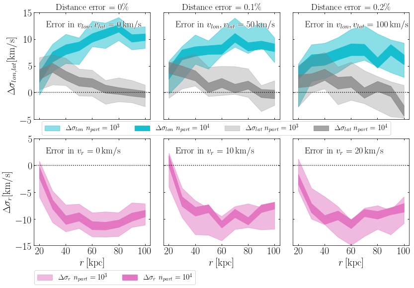
Figure 20: Relative difference of the velocity dispersion between different regions in the sky in a given velocity component, $\Delta\sigma$, as a function of Galactocentric distance. Regions 1-8 are used for measuring $\Delta\sigma_{r}=\sigma_{r|region1-7}-\sigma_{r|region8}$ and 9 to 10 for measuring $\Delta\sigma_{lon,lat}=\sigma_{lon,lat|region9}-\sigma_{lon,lat|region10}$ as defined in Table  6. We use these regions for distances from 20 to 100 kpc. These regions are associated with the location of the Transient response (top panels: cyan, $\Delta\sigma_{lon}$; and gray, $\Delta\sigma_{lat}$) or the Collective response (bottom panels: magenta, $\Delta\sigma_{r}$) relative to an unassociated region, as marked in Figure 19 (solid and empty boxes; 20 square degrees, 5 kpc in thickness). Each region is sampled using $10^{3}$ and $10^{4}$ particles. The width of each line corresponds to the 1$\sigma$ deviation about the mean using $10^{3}$ and $10^{4}$ particles, computed using the bootstrap technique. Errors in distances and velocities are included as marked above each column. Results for Model 1 and Model 2 are similar; here, we show only results for Model 1. $\Delta\sigma_{lon}$ illustrates that $\sigma_{lon}$ is boosted in the regions surrounding the Transient response. But, in the same region of the sky, $\Delta\sigma_{lat}$ is expected to display distinctly different behavior, remaining similar to the average dispersion at all distances. $\Delta\sigma_{r}$ is measured in the expected “cold region” associated with the Collective response, which demonstrates velocity dispersions 10 km/s lower than average. This ratio is expected to persist over a huge distance range of 50 kpc and should be largely unaffected by velocity and distance errors. We conclude that the kinematic impact of the LMC on the smooth component of the stellar halo should be observable even when large uncertainties are included.

5.3 Sampling Stars in the Stellar Halo

Observing the MW’s DM halo wake in the stellar halo is not an easy measurement. There is likely substructure and the stellar density is expected to decrease in the outer halo.

Here, we estimate the expected number of stars in the stellar halo from recent measurements of the stellar halo number density profile from RR Lyrae and K-giants. Note that the K-giant density profile (Xue et al., 2015) drops faster than the RR Lyrae profile (Hernitschek et al., 2018), see Figure 4. This trend is also in agreement with BHB stars (Deason et al., 2014, 2018).

We use these profiles to estimate the number of stars at a given distance assuming that the stellar halo is homogeneous and is either entirely made up of RR Lyrae or K-giants. With such assumptions, the number of stars $N_{star}$ in a spherical shell of thickness $dr$ is

$$N_{\star}(r,r+dr)=\frac{\rm{M}_{\star halo}\int_{r}^{r+dr}\nu(r)}{\rm{M}_{\star}\int_{0}^{R_{obs}}\nu(r)r^{2}dr},$$ (15)

where $\nu(r)$ is the observed density profile, $R_{obs}$ is the radius to which the stellar halo extends (here we assume 90 kpc), and $\rm{M}_{\star halo}$ is the total mass of the stellar halo. Note that the normalization factor in Equation 15 is $M_{\star halo}/M_{\star}\int_{0}^{R_{vir}}\nu(r)r^{2}dr$. Where $\rm{M}_{\star}$ is the mass of a K-giant. Figure 21 shows the number of stars inside a 20 square degree field of 5 kpc thickness, as marked by boxes in Figure 17 and 19, as a function of distance for the RR Lyrae (black lines) and the K-giants (cyan lines) using three stellar halo masses $10^{7}$, $10^{8}$, and $10^{9}$ M_⊙. Figure 21 illustrates that, assuming that finding 100 or 1000 particles in a volume of $20$ square degree and 5 kpc thickness in the stellar halo is consistent with current observations of the number density profile, finding $10^{4}$ stars could be possible if the total mass of the stellar halo is larger than $10^{8}$ M_⊙.

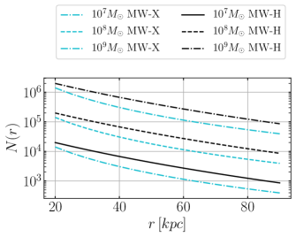
Figure 21: Number of stars, $N(r)$, within regions with the same volumes as the observational fields in Figure 17 and 19 (20 square degrees, and thickness of 5 kpc). The cyan and black lines indicate the expected number of stars in such a volume using the observed number density profiles for the stellar halo for K-giants (MW-X Xue et al., 2015) and RR Lyrae (MW-H Hernitschek et al., 2018), assuming different normalizations for the total mass of the stellar halo, as marked. In Figure 18, we sample the observational fields using 100 and 1000 particles, which is well below the expected total number of stars in the stellar halo in the same volume at the same distances. In Figure 20, we increased the sampling to $10^{4}$ stars, which was found to be reasonable if the mass of the MW’s stellar halo was in excess of $10^{8}$ M_⊙.

6 Discussion

Here, we discuss the details of our simulation suite and place our results in a broader context. In §6.1, we study the convergence of our simulations and predicted observable signatures. We then explore how our results change as a function of LMC mass in §6.2. In §6.3, we compare the strength of the perturbations of the MW’s DM halo from the Sgr. dSph to those from the LMC. We consider how the Transient response can be distinguished from the stellar counterpart of the Magellanic Stream in §6.4 and discuss how the properties of the wake can be used to constrain the mass of the MW in §6.5. Finally, in §6.6, we discuss how our results can be used to constrain the nature of the DM particle.

6.1 Convergence of the Simulations

In this section, we discuss the convergence of our simulations. Specifically, we demonstrate that the chosen number of particles in our simulations is sufficient to capture the DM halo response and to measure relative changes in the velocity dispersion.

The DM wake is governed by resonances induced by the LMC, as discussed in detail in Weinberg (1998a) and Choi et al. (2009). In particular, Weinberg & Katz (2007) discuss that capturing these resonances in an $N$-body simulation primarily depends on the number of particles used. For a satellite-host interaction with mass ratios of 1:10, Choi et al. (2009) showed that $10^{6}$ particles with equal mass for the host satellite is sufficient to capture the resonances in MW-like DM halo. However, to fully capture the innermost and low-order-resonances a $10^{8}$ halo is needed. Therefore, our $10^{8}$ equal-mass particles should also capture the resonant nature of the MW-LMC interaction; we test this statement in detail below using the fiducial LMC model with $\rm{M}_{vir}=1.8\times 10^{11}\rm{M_{\odot}}$ orbiting within an isotropic MW halo (Model 1).

Figure 22 illustrates the morphology of the DM wake generated in using the same set up as in Sim. 4 (most massive LMC; Model 1 halo) but for three different resolutions ($10^{6}$, $4\times 10^{7}$, $10^{8}$ particles) in a Mollweide projection inside a spherical shell of 5 kpc width at 45 kpc. The density contrast is defined relative to the MW modeled in isolation with the same resolution (Equation 9; Figure 7). The figure shows that in the lowest-resolution case (left panel) the structure of the DM wake is barely discernible. In the higher resolution simulations (the middle and right panels) the structure of the DM wake is clear and is almost identical in both cases, illustrating qualitative convergence.

Figure 23 shows the stellar number density ratio between the underdense and overdense regions associated with the LMC’s DM wake as a function of radius. The regions chosen to compute the density ratios have the same volumes as those in Figure 18, whose properties are listed in Table 6. The shaded regions show the errors in the measurements computed using the bootstrapping technique. As the resolution increases, convergence is achieved within 10%, indicating that results presented in Figure 18 are reliable.

In Figure 24 we show that the predicted ratio in radial-velocity dispersion, $\sigma_{r}$ (as in the bottom panel of Figure 20), is similarly converged. If one computes the radial-velocity dispersion in smaller regions of the halo, the errors will be larger but the mean values are unchanged. These results for $\sigma_{r}$ are also consistent for the other components of the velocity dispersion: $\sigma_{\theta}$ and $\sigma_{\phi}$.

We conclude that the results for the density and the kinematics of our simulations with $10^{8}$ particles are converged and that the high number of particles allows us to predict the morphological and kinematic properties of the DM wake and the halo response with small numerical uncertainties.

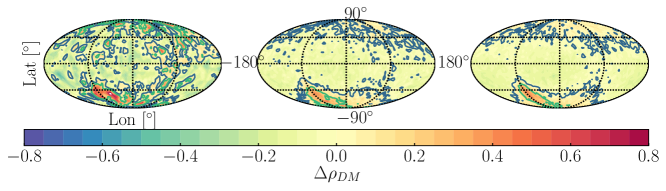
Figure 22: Mollweide all-sky map of the change in DM density in a spherical shell (5 kpc in thickness at 45 kpc) using the same set up as Sim. 4 (most massive LMC; Model 1 halo). The density contrast is measured relative to MW Model 1 in isolation ($\Delta\rho_{DM}$; Equation 9). Contours are defined as in Figure 7. Plotted are results for three versions of Sim 3., using different resolutions: $10^{6}$ particles (left), $4\times 10^{7}$ (middle) and $10^{8}$ particles (right). The overdensities were computed in a cell of size $(3.6^{\circ})^{2}$ in all cases. The low resolution simulations cannot resolve the details of the DM halo response, while the higher resolution simulations show similar morphology, illustrating qualitative convergence.

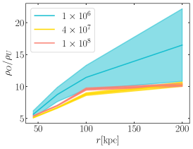
Figure 23: Density ratio between two regions with the same size of those defined in Table 6 for halos of an isolated MW. The different lines show the results for three simulations with different resolution (number of particles as marked in the legend). The shaded areas represent the 1$\sigma$ error on the measurements computed using bootstrapping. The density ratio converges for the two higher resolution simulations (red and yellow lines).

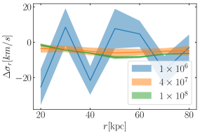
Figure 24: The relative radial velocity dispersion, $\Delta\sigma_{r}$, profile computed in the same regions as those defined in Table 6 for three simulations with different resolution (colored lines). The width of the lines show the $1\sigma$ errors in $\sigma_{r}$ computed using the bootstrapping technique. Convergence is achieved within 5 km/s for the two higher resolution simulations.

6.2 The Impact of the Mass of the LMC

In this section, we study how our results scale with the total halo mass of the LMC at infall. So far, our analysis has focused on the fiducial LMC mass model (LMC3) of $\rm{M}_{vir}=1.8\times 10^{11}$M_⊙. However, as discussed in §2, the total mass of the LMC is unknown within a factor of three. We created 8 simulations with lighter and heavier LMC masses, see Table 3, to study how the velocity dispersion and the strength of the DM wake are affected by the LMC’s infall mass.

Figure 25 shows how key observables associated with the LMC’s DM wake scale as a function of the LMC mass. The right panel shows the strength of the Transient response (overdense region) as a function of LMC mass and at different distances. Each line shows the ratio in density between the same regions identified in Table 6 and plotted in Figure 18. One region is always coincident with the Transient response (overdense region, $\rho_{O}$) and the other is in an expected underdense region adjacent to the wake ($\rho_{U}$).

The strength of the Transient response increases as a function of LMC infall mass in the outer halo, from 15% at 70 kpc, up to 45% at 200 kpc. Interestingly, at 25 kpc and 45 kpc the strength of the wake is similar for all LMC mass models. These results suggest that the Transient response created at 45 kpc and the weaker signals in the inner halo should be present regardless of the assumed LMC mass. Furthermore, we confirm that the morphology of the Transient and Collective DM responses are the same for all LMC mass models, despite minor differences in their exact orbital trajectories.

The left panel of Figure 25 illustrates the ratio in the radial velocity dispersion, $\Delta\sigma_{r}$, between the same two regions on the sky used in §5.2 and Figure 20 to observe the ‘cold region’ in the north associated with the Collective response. The results presented here are for the DM particles, but trends are the same using stellar particles. Each line shows the value of $\Delta\sigma_{r}$ as a function of Galactocentric distance for different LMC masses (Sim. 1 through 4). As the mass of the LMC increases, $\Delta\sigma_{r}$ becomes increasingly negative. This region of the sky (the Collective response) is impacted by both halo resonances and the COM motion of the disk relative to the outer halo, both of which increase in strength with increasing LMC mass. Similar trends were found by Laporte et al. (2018b) for the strength of the warp in the MW’s stellar disk owing to the LMC.

These results suggest that (1) the strength of the decrease in radial velocity dispersion in the “cold region”; and (2) the magnitude of the bipolar radial-velocity signal in the outer halo (redshifts in the north and blue shifts in the south; Figure 10 and 11), can together constrain the total mass of the LMC at infall.

In the inner regions of the halo, 20 and 30 kpc, $\Delta\sigma_{r}$ does not change as much with LMC mass as in the outer halo. This is expected since the LMC’s pericenter distance is at $\sim$ 45 kpc; this, its impact is not as strong in the inner regions of the halo. In addition, the COM motion of the inner halo is following that of the disk. We found similar results for $\sigma_{\theta}$ and $\sigma_{\phi}$.

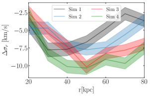
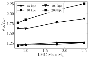
Figure 25: Left panel: ratio of the radial-velocity dispersion, $\Delta\sigma_{r}$, computed in the same magenta regions as marked in Figure 19. This choice highlights the ‘cold region’ in the north associated with the Collective response, which exhibits lower radial dispersion (see Figure 9). As such, $\Delta\sigma_{r}$ is negative. The colored lines show the results for simulations with different LMC infall masses (Sim. 1-4; see Table 3). As the mass of the LMC increases, the response grows in strength, becoming increasingly negative. However, the ratio is always decreasing from 20 to 40 kpc, regardless of LMC infall mass. Right panel: density ratio between regions on the sky that are coincident with the DM wake (overdense; O) and adjacent to the wake (underdense; U), as a function of LMC mass. The selected regions are the same as those in Figure 17. Different symbols mark results at different Galactocentric radii. As the mass of the LMC increases, the density contrast grows at all radii. The change is modest for the smallest radii (25 and 45 kpc), suggesting that perturbations in the inner halo will exist irrespective of the LMC’s infall mass.

Note that we have characterized the LMC’s wake ignoring the Small Magellanic Cloud (SMC). However, the SMC is roughly one-tenth of the stellar mass of the LMC. We expect that the inclusion of the SMC might make the structure of the wake more complicated, since the SMC is modifying the DM halo density profile of the LMC as it orbits within it. Nevertheless, the SMC’s orbit largely traces the COM motion of the LMC (Kallivayalil et al., 2013). Its impact is most likely captured by increasing the mass of the LMC, which we have characterized here. We thus do not anticipate that our conclusions about the morphology and kinematics of the LMC’s wake will change with the inclusion of the SMC.

6.3 Density Perturbations from both Sgr. & the LMC

We claim that the LMC is currently the strongest perturber of the MW’s DM halo at r$>$45 kpc. The LMC is currently the MW’s most massive satellite and recently passed its first pericenter approach $\sim 50$ Myr ago. However, the LMC is not the only satellite that has perturbed the MW’s DM halo. Sgr. has been orbiting the MW for at least the past 6 Gyr, having made at least three pericenter approaches at $\sim$ 20 kpc and apocenter distances of $\sim 100$ kpc (Dierickx & Loeb, 2017; Fardal et al., 2019; Laporte et al., 2018b).

Fortuitously, the orbital plane of Sgr is perpendicular to that of the LMC. This means that the DM wake induced by Sgr is likely in different regions of the sky than that of the LMC. However, understanding the complex interplay between these two effects requires N-body simulations.

Here, we compare the perturbations to the MW’s DM halo from both the LMC and Sgr. We use the simulations presented in Laporte et al. (2018b), a suite of two $N$-body simulations of the interaction between the MW, LMC, and Sgr and four additional simulations of the MW-Sgr interaction alone (no LMC). These simulations were used in Laporte et al. (2018b) to quantify the impact of these satellites on the MW’s disk.

The MW and LMC models used to generate these simulations are the same as those presented in this work. Four different models for the mass of Sgr. are used (see Table 1 in Laporte et al., 2018b). For this study, we use the most massive Sgr. model, with a mass of M${}_{200}=$1$\times$10¹¹M_⊙ and concentration $c_{200}=26$ at infall, since this massive and concentrated model should generate the strongest DM wake. In the following, we use the MW-LMC-Sgr and MW-Sgr simulations to compare the amplitudes and morphology of the DM wakes induced by Sgr. and the LMC at the present day.

The left column of Figure 26 shows the ratio of the local DM overdensities relative to the all-sky average, highlighting the DM wake produced by Sgr alone at different Galactocentric distances. The middle column shows the same for the combined DM wakes from both Sgr and the LMC. The right column shows the ratio of the DM density perturbations from both Sgr+LMC to the response to Sgr alone (middle column/left column). The present-day halo response to Sgr alone is predominantly found at $lon=0^{\circ}$ and at $(lat=0^{\circ},lon=\pm 180^{\circ})$, as expected given its orbital plane and the location of the Sgr. Stream (Figure 17). However, Sgr Transient response was stronger in the past and it has decayed over time.

The overdensities produced by the halo response to the motion of Sgr are up to 30% relative to the mean DM density of the halo and can be observed from 25 to 200 kpc. However, in the presence of the LMC, the halo response to Sgr is barely discernible. The similarity between the middle (LMC+Sgr) and right columns (Sgr’s contribution removed) illustrates that the LMC’s contribution dominates and that Sgr does not change the morphology of the LMC’s DM wake at $r>25$ kpc, However Sgr could dominate in the inner halo (Laporte et al., 2018b).

Interestingly, Sgr’s DM wake does affect the density ratios between the underdense and overdense regions created by the LMC’s DM wake. In the most extreme case, the ratio could decrease up to $\sim$ 12%, which is not sufficient to significantly modify the expected signal form the LMC’s DM wake. We conclude that our results presented in §4 are still valid in the presence of Sgr.

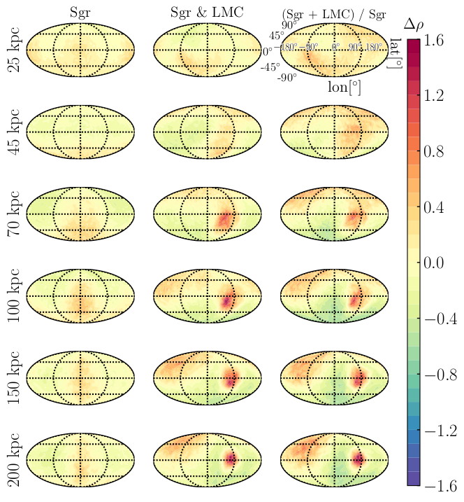
Figure 26: The present-day DM halo response of an isotropic MW DM halo to the orbits of the Sagittarius dwarf spheroidal (Sgr.) and the LMC after 6 Gyr of evolution. Sgr.’s infall mass is M${}_{200}=1\times 10^{11}$M_⊙ with a concentration of $c_{200}=26$. These results are based on the simulations of Laporte et al. (2018b). The color bar indicates the ratio of the local DM density to the all-sky average, $\Delta\rho_{DM}$. Only MW DM particles are included in all panels. Different rows indicate different Galactocentric radii. Left column: the present day response of the MW’s halo to the orbit of Sgr alone. Middle column: same as left column, but also including a massive LMC ($2.5\times 10^{11}$M_⊙; LMC4), which enters the MW virial radius $\sim$2 Gyr ago. Right panel: ratio of the present day wakes from Sgr.+LMC to that of Sgr. alone (middle column/left column). The LMC clearly dominates at all distances, wiping out the response to Sgr. In particular, the orbit of Sgr. does not affect the morphology of the LMC’s DM wake. We conclude that our results are robust to the presence of Sgr.

In addition, as in the case with Sgr, the LMC can erase the previous signatures in the outer halo of earlier merger events due to its recent and ongoing infall.

6.4 Distinguishing the Magellanic Stellar Stream from the stellar Transient response.

We have discussed the observability of the stellar Transient response in previous sections. However, the existence of a stellar component of the Magellanic Stream (MS) has also been predicted by all tidal models of the Magellanic System (e.g. Gardiner & Noguchi, 1996; Diaz & Bekki, 2012; Besla et al., 2013). How might the stellar MS be distinguishable from the stellar Transient response? In this subsection, we discuss the differences in the location, density, kinematics, and chemistry between the stellar MS and the Transient response.

The Transient response is expected to be well-aligned with the past orbit of the LMC on the plane of the sky. In contrast, the proper motion of the LMC (Kallivayalil et al., 2013) indicates the past orbit of the LMC is not aligned with the gaseous MS on the plane of the sky (Besla et al., 2007). Note, however, that the gas and stellar MS may also not be spatially coincident. The gaseous MS is subject to hydrodynamical forces such as gas drag and ram pressure (Mastropietro et al., 2005), owing to its motion through the Circumgalactic Medium, which may create offsets (e.g. Roediger & Brüggen, 2006). Together, this suggests that the, yet undiscovered, stellar component of the MS is expected to be neither coincident with the LMC’s orbit (Diaz & Bekki, 2012; Besla et al., 2013; Guglielmo et al., 2014; Pardy et al., 2018) nor the Transient response.

The predicted locations of the stellar MS, the LMC orbit and the stellar Transient response are illustrated in Figure 27 at Galactocentric distances greater than 70 kpc, where the expected deviation of the LMC’s orbit from the location of the MS on the sky is more pronounced. The plotted stellar MS model is from the Model 1 simulation of Besla et al. (2013), which simulates the interaction history between the SMC, LMC, and the MW, tracking the tidal stripping of stars and gas from the SMC.

This figure illustrates that the stellar Transient response is expected to be much more extended along and across our line of sight than the stellar MS.

At every radius, the width of the stellar Transient response is at least five times the width of the stellar MS. These results show that, overall, the stellar MS is expected to have little overlap spatially with the stellar Transient response.

The spatial offset of the MS from the LMC orbit is explainable by the MS originating from tidal stripping of the SMC, which is initially modeled as a rotating disk whose orbit does not exactly track that of the LMC. Because the stellar MS is expected to originate from the SMC, the chemistry of any detected stars will likely be the most important discriminant between the stellar Transient response and the stellar MS, the former being comprised of old halo stars.

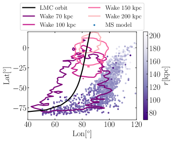
Figure 27: Projection of the location of the stellar Transient response and the stellar Magellanic Stream (MS), from Besla et al. (2013) (their Model 1; purple points), in Galactocentric coordinates. The color scale indicates the Galactocentric distance to stellar particles modeled in the MS. The contours shows the stellar density enhancement of the MW halo ($\Delta\rho$, as defined in Equation 9) for our Sim. 7 (Model 2 halo and most massive LMC model), at different Galactocentric distances. The contours are at 0.25, 0.6, 0.75 and 0.7 for distances 70, 100, 150, and 200 kpc, respectively. The stellar transient response is seen as an overdense region that tracks the LMC’s past orbit (black solid line). The stellar MS is thinner than the stellar Transient response and spatially offset from both the LMC’s orbit and the Transient response.

We further find that the density of stars in the modeled MS is higher than the predicted density of the stellar Transient response at every Galactocentric distance by at least 1 to 2 orders of magnitude. This may complicate searches for the stellar Transient response. We caution that different authors find strong variations in the predicted density of the stellar MS (e.g., Diaz & Bekki, 2012; Pardy et al., 2018). Also, the expected stellar density of the Transient response is very sensitive to the assumed stellar halo density profile.

In addition to the differences in the spatial distribution and density of the stellar MS, we also expect differences in the kinematics. Stellar streams display kinematically coherent motion in the direction of the progenitor (see Sacchi et al.2019, in preparation). Given the polar orbit of the stellar MS, its kinematic signature is expected to be the strongest in $\overline{v_{r}}$, $v_{lat}$ and $\sigma_{lat}$. This is the opposite of the stellar Transient response, which is characteristically surrounded by converging/diverging flows in $v_{lon}$ and increases in $\sigma_{lon}$ with minimal impact on $\sigma_{lon}$ or $v_{lat}$ (§4).

In summary, while the stellar MS is expected to be denser than the stellar Transient response, the latter is expected to be spatially offset, thicker, and chemically distinct from the stellar MS. The stellar Transient response is also characterized by converging and diverging stellar motions, whereas stellar streams display motions along the stream toward the progenitor. We conclude that it will be possible to distinguish the detection of the stellar Transient response from the stellar MS.

6.5 The Transient response as an Indirect Measure of the MW’s Total Mass.

The past orbit of the LMC is strongly influenced by the total mass of the MW. As the mass of the MW increases, the orbit of the LMC becomes more elliptical, allowing the LMC to complete one or more orbits about the MW within a Hubble time (Kallivayalil et al., 2013). Unlike stellar streams, which can deviate substantially from the past orbital path of a progenitor disk galaxy, the Transient response thus uniquely traces the orbit of the LMC. This provides us with an indirect probe of the underlying DM distribution of the MW.

In particular, if the virial mass of the MW is of the order of $1.5\times 10^{12}$ M_⊙, the LMC will have traversed through the northern sky (Patel et al., 2017b), leaving a very different signature in the stellar halo than that illustrated here. If the mass approaches $2\times 10^{12}$ M_⊙, the LMC may make multiple orbits, in which case, as illustrated in the case of Sgr (§6.3), the Transient response will likely be very difficult to identify.

As such, by detecting the amplitude, sky location, and distance of the LMC’s Transient response, we can constrain the 3D orbital path of the LMC, which in turn will constrain the mass profile of the MW’s DM halo.

6.6 Prospects of Studying the Nature of the DM Particle Using the LMC’s DM Wake

In the era of high-precision astrometry, surveys like LSST and DESI will reveal the structure and kinematics of the stellar halo out to 300 kpc (Ivezić et al., 2008). These large-volume data sets have the capability to reveal the shape and density structure of the DM halo. But it is less clear how they may inform us about the nature of the DM particle itself.

In this work, we have outlined a strategy for observing the signatures of the DM wake induced by the LMC in the kinematics and density profile of the stellar halo over a large range of Galactocentric distances. Identifying these signatures will both constrain the total infall mass of the LMC and provide proof of dynamical friction in action, which in turn requires the existence of a DM particle. Furthermore, here we discuss how the properties of the wake itself may reveal the characteristics of the DM particle.

We have shown that for the CDM scenario, the morphology of the LMC’s wake is largely independent of both the mass of the LMC and initial MW halo kinematics (Model 1 vs. Model 2). However, both of these factors do affect the amplitude of the halo response. As such, the amplitude of the wake may allow us to constrain the anisotropy profile of the MW’s halo, given independent probes of the LMC’s mass (e.g., Erkal et al., 2019). The anisotropy profile is a significant uncertainty in the expected velocity distribution of DM particles in the solar neighborhood, particularly the high velocity-tail (Besla et al 2019, in preparation), which has direct consequences for direct detection experiments (Green, 2002a, b).

In the CDM framework, the location of the LMC’s DM wake on the sky is controlled primarily by the orbit of the LMC over the past 1 Gyr. Each MW+LMC model explored in this study resulted in final LMC position and velocity vectors that are not exactly the same, but all agree within 2$\sigma$ with the measurements of Kallivayalil et al. (2013), see Figure 28. Over the short timescale considered in this study, uncertainties in MW mass cause only minor changes to the orbit (Kallivayalil et al., 2013). In particular, changes to MW mass will not change the projected location of the LMC’s orbit on the sky (Besla et al., 2007). We thus conclude that our predictions for the general shape and location the LMC’s wake are robust within the CDM framework owing to the current low uncertainties in the LMC’s 6D phase-space properties.

It is possible, however, that different DM models may affect the location and morphology of the DM wake on the sky in a manner distinct from the uncertainties in the LMC orbit. If the DM is self-interacting (SIDM) and velocity-independent, we might not expect large differences from the wake in the CDM model. Upper limits in the cross-section of SIDM particles already suggest that the interaction between particles might not be as strong to create difference in the wake. However, if the interactions of the DM particles are velocity-dependent the relative velocity difference between the LMC and the MW DM halo could be sufficient to produce a significant deviations in the morphology and strength of the wake, relative to the CDM case.

On the other hand, if the DM is Fuzzy (FDM), i.e. composed of light bosons or axion particles, the properties of the DM wake will also be different than in the CDM model. For example, Hui et al. (2017) showed that the orbital decay times of globular clusters in the Fornax dwarf galaxy are longer in the FDM model. In FDM, the DM halo is cored, rather than forming a cusped as in CDM, which changed the density and velocity dispersion of the DM halo. Read et al. (2006) showed that dynamical friction behaves differently within DM cores vs. in cusps. In DM cores, a satellite initially undergoes a rapid strong dynamical friction followed by suppression of dynamical friction. In addition, Hui et al. (2017) showed that the dynamical friction is different in FDM, since the de Broglie wavelength of the FDM particles has to be taken into account.

Early works by Furlanetto & Loeb (2002) compared the structure of the overdensity associated with DM wakes in CDM and SIDM, which they approximated as a perfect fluid. They found that the structure of the wake is more complicated in SIDM. For example, the wake structure can change if the satellite galaxy is moving subsonically or supersonically. In the subsonic case, the wake is symmetric in front of and behind the satellite. In the supersonic case, the wake forms a Mach cone trailing the satellite. Furthermore, in these simulations, DM was subject to ram-pressure, which creates an additional DM wake, and a bow shock in the supersonic case. These studies already show large differences in the structure of the wake in different DM models. We now have stronger constraints on the nature of the DM particle, and hence new $N$-body simulations revisiting the structure and morphology of DM wakes in different DM models are missing.

In particular, the interaction between the MW and the LMC in such alternative DM models, including a live stellar halo, are required in order to make concrete predictions of the morphology of the DM wake and the observable counterpart in the stellar halo. This will be the subject of future work.

6.7 Effect of the MW’s initial Dark Matter density profile

In this study, we have modeled the MW’s initial DM density distribution using a Hernquist profile. The kinematics of the DM halo will be different if the density profile changes - as such, the resonant response of the DM halo can also change. The minor differences exhibited between our adopted Model 1 and Model 2 kinematic profiles suggest that such differences will not significantly modify the morphology of the halo response, but may impact the amplitude of the perturbations. Preliminary work studying the halo response to the LMC using an NFW profile suggests that the overall morphology and kinematics of the wake are qualitatively similar to the results shown in this study (M. Weinberg 2019, private communication). As such, we expect that uncertainties in the mass of the LMC are the dominant source of uncertainty in the predictions presented in this study.

7 Conclusions

Since its first entry within the MW’s virial radius, $\sim 2$ Gyr ago, the LMC has been the most massive perturber of the MW’s DM and stellar halo. Yet, the strength, nature, and location of these perturbations has remained unknown. In this work, we quantified the density and kinematic perturbations induced within the MW’s DM and stellar halo using high-resolution $N$-body simulations of the recent pericentric approach of a massive LMC ($8-25$ $\times 10^{10}$ M_⊙).

The ultimate goal of this study is to characterize global patterns in the stellar halo kinematics and densities that are correlated with the orbital motion of the LMC. When taken together, these signals can confirm the identification of the LMC’s DM wake. Given the rarity of LMC analogs at pericentric approach about MW analogs in cosmological simulations, studying this process in detail necessitates the use of controlled $N$-body simulations. In this work, we presented a suite of 8 $N$-body simulations, with four different LMC masses (8, 10, 18, 25 $\times 10^{10}$ M_⊙) and two MW models with the same mass ($1.2\times 10^{12}$ M_⊙), but with different kinematic structure. MW Model 1 has an isotropic anisotropy parameter ($\beta=0$) while Model 2 has a radially biased anisotropy parameter (Eq. 1). In all simulations, the final position and velocity of the simulated LMC is ensured to be within 2$\sigma$ of the current measured values (Kallivayalil et al., 2013). In order to describe the wake structure as observables, we include a MW stellar halo that was constructed by assigning weights to the MW DM particles’ masses and velocities in order to reproduce the observed MW density profiles.

We identify global changes in the density and kinematics of the stellar halo that persist over large Galactocentric distances (40-200 kpc). Specifically, we identified three main components of the wake generated by the LMC. The Transient response, trailing the LMC and following the orbital history of the LMC out to the virial radius of the MW. The Collective response, in the Galactic north, leading the LMC; and the The Global Underdensity, an underdense region surrounding the Transient response mainly in the south and extending out to the virial radius of the MW.

We find that the density enhancement associated with the Transient response is stronger in Model 2 at every distance, reflecting the resonant nature of the halo response. The Collective response on the other hand, has a different morphology in both models and its associated density enhancement is stronger in Model 1. We conclude from these results that the initial kinematic state of the MW affects the strength and the morphology of the wake, and that deviations from isotropic models can strengthen the wake.

The kinematics and density distribution of the MW’s stellar halo are found to be perturbed by the LMC and correlated with the location and properties of the DM wake. Below, we summarize our main results for the stellar counterpart to the Transient and Collective DM responses generated by the LMC:

1. Overdensities Associated with the Transient response are stronger at distances larger than 45 kpc. The Transient response should be detectable as an overdense region with respect to underdense regions if at least 20 stars are identifiable within a 20 square degree area, 5 kpc in thickness (corresponding to stellar number densities of $\sim$0.01-0.03 kpc^-1) (Figure 18). Such number densities are consistent with measurements of the number density profile of RR Lyrae and K-Giants. At distances greater than 70 kpc, the strength of the Transient response increases with increasing LMC infall mass, but is largely independent of LMC mass at smaller radii. The Transient response is not found to be coincident with known halo substructures - in particular, regions of the Transient response can be found that avoid the Sagittarius Stream.

2. Radial velocities: The mean radial stellar velocities show a bipolar behavior. Overall, stars in the Galactic north are moving away from the disk (redshifts), while stars in the south are moving toward the disk (blueshifts). This is most clearly predicted at distances larger than 45 kpc (see Figure 10). This bipolar behavior is indicative of the barycenter movement of the disk due to the gravitational acceleration from the LMC (Gómez et al., 2015). Correspondingly, the strength of this velocity shift will scale with the infall mass of the LMC. This behavior is associated with the Collective response and should be observable in ongoing or upcoming radial velocity surveys.

3. Radial velocity dispersion: In the north, there is a decrease in the radial velocity dispersion of $\sim$10 km/s that we call the “Cold region”. This region is also located within the Collective response and corresponds to a region of the sky where the LMC has not yet passed through, but will in the future. Stars in the “Cold region” have smaller mean radial velocities than stars in other regions in the north. The “Cold region” persists over a large distance range, from 45 kpc to the virial radius, and large area on the sky. This structure should also be observable in radial velocity surveys (see Figure 20).

4. Tangential motions in the vicinity of the LMC: There are flows of stars converging towards the LMC. This is apparent in both latitudinal and longitudinal velocity components in the vicinity of the LMC. This motion is associated with an increase in the velocity dispersion in both components. However, the observability of such motions will be complicated owing to the extended stellar populations associated with the Magellanic Clouds.

5. Motions along the Transient response: In the latitudinal tangential direction, stars within the Transient response follow the orbital direction of the LMC’s COM (Figures 12 and 13). In contrast, in the longitudinal tangential direction, we find diverging flows, where stars that were once converging toward the LMC (see previous point) have already crossed each other and now are going in opposite directions (Figures 14 and 15). Consequently, the latitudinal velocity dispersion is enhanced in the regions surrounding the Transient response, and decreased within it. In contrast, the longitudinal velocity dispersion is unaffected. This opposite behavior is expected to be observable from 70 to 100 kpc, provided that the tangential motions of at least $10^{3}$ RR Lyrae or K-Giant stars are measured within a 20 square degree region, 5 kpc in thickness, and tangential velocity errors are less than 100 km/s. Such accuracies are expected to be plausible with LSST. Furthermore, within the Transient response, the radial velocity dispersion is expected to be decreased relative to the average. The Transient response can thus be identified by these correlated, opposite kinematic signals in velocity dispersion.

6. The anisotropy parameter, $\beta$: is affected in all regions of the sky, as a result of the perturbations in all components of the velocity dispersion. We found that changes in $\beta$ are largest in the isotropic MW model (Model 1) but are still present in the radially anisotropic Model 2. The strongest changes in $\beta$ are found to be from -0.4 up to 0.35 at 45 kpc. At larger distances, the Transient response is discernible in the $\beta$ maps (see Figure 16).

7. The stellar counterpart of the Magellanic Stream is expected to be distinguishable from the Transient response, through its differing kinematics, spatial offset from the LMC orbit (which the Transient response tracks) and its chemical composition. The stellar stream will be comprised of SMC stars, whereas the Transient stellar response will be comprised of older halo stars.

8. The halo response to the orbit of a massive Sagittarius dwarf spheroidal is insufficient to wipe out the perturbations induced by the LMC (see Figure 26). This suggests that our results are robust to perturbations from cosmological substructure, but this must be tested in a cosmological setting and is the subject of future work.

Given the imminence of the era of all-sky photometric and kinematic surveys of the stellar halo to large distances, we are optimistic that the Transient and Collective response induced by the recent passage of the LMC through the stellar and DM halos will be detected. Indeed there are few regions of the sky where the density and/or kinematics of the stellar halo are not expected to be impacted by the LMC.

Ultimately, the detection of the Transient response will track the past orbit of the LMC and constrain the eccentricity of that orbit, which is an indirect measure of the total mass of the MW. Owing to the expected dependence of dynamical friction to the properties of the DM particle, the kinematics and density signatures of the halo response will provide an indirect measurement and a new test bed of the nature of the DM particle.

Appendix A Simulation details

Here, we present details of our simulations. Table 8 lists present-day positions and velocities of the LMC in our simulations with respect to the observed values from Kallivayalil et al. (2013) (Columns 4-9). We also show the initial condition coordinates in Column 10. All of the simulations are within 2$\sigma$ of the total position and velocity vectors, as shown in the right-most columns of ($\Delta v$ and $\Delta r$). However, three simulations exceed 2$\sigma$ in their present-day $\hat{z}$ coordinates, and all of the simulations have difficulty exactly matching the $\hat{v}_{y}$ component.

Table 8: Summary of LMC-MW simulations. Initial conditions list the position and velocity vectors of the LMC at infall, $\sim$2 Gyr ago. $\Delta x,y,z,v_{x},v_{y},v_{z}$, denote the difference in each component of the present-day 3-D position and velocity vectors with respect to the measured values found in (Kallivayalil et al., 2013).

Sim.	MW model	LMC model	$\Delta x$ [kpc]	$\Delta y$[kpc]	$\Delta z$ [kpc]	$\Delta v_{x}$ [km/s]	$\Delta v_{y}$ [km/s]	$\Delta v_{z}$ [km/s]	Initial Conditions:
1	Model 1	LMC1	1.75	2.68	2.56	-5.04	-55.17	7.65	$\vec{r}=(27,276,57)$ , $\vec{v}=(7.22,-61,-78)$
2	Model 1	LMC2	1.94	1.69	3.89	-20	-47	15	$\vec{r}=(28,310,90)$ $\vec{v}=(7,-35,-70)$
3	Model 1	LMC3	2.12	0.61	1.99	-4.47	-42.65	1.53	$\vec{r}=$ (12, 238, 130) $\vec{r}=$(12, 13, -77)
4	Model 1	LMC4	-0.16	1.19	4.92	-5.99	-38.49	19.61	$\vec{r}=$(11.58, 248, 130) $\vec{v}=$(12, 11, -77)
5	Model 2	LMC1	-0.13	2.68	-1.21	-0.19	-55.74	1.03	$\vec{r}=$(24, 278, 58), $\vec{v}=$(4, -59, -77)
6	Model 2	LMC2	2.31	2.54	-0.5	-12.07	-50.89	7.86	$\vec{r}=$(28, 306, 90) $\vec{v}=$(7, -35, -70)
7	Model 2	LMC3	2.66	-0.4	0.07	1.66	-36.59	0.81	$\vec{r}=$(12, 238, 130) , $\vec{v}=$(12, 13, -77)
8	Model 2	LMC4	2.69	0.46	3.21	-2.42	-35.56	19.34	$\vec{r}=$(11, 238, 130) , $\vec{v}=$(12, 11, -77)

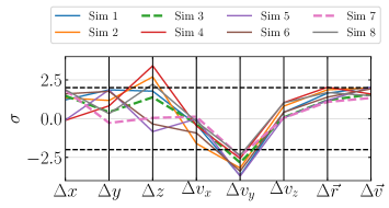
Figure 28: Final phase space coordinates of the LMC in all simulations. The y-axis shows the deviation of each simulated LMC position and velocity component at the present day from that observed by Kallivayalil et al. (2013). The black dashed horizontal lines indicate a 2$\sigma$ deviation from the observations.

Figure 28 shows the final phase-space coordinates of the eight LMC+MW simulations described in Table 3. The magnitude of the position and velocity vectors are all within 2$\sigma$ of the observations. Most of the individual velocity and position components are also within 2$\sigma$ of the observations (dashed lines). However, three simulations exceed 2$\sigma$ in the $\hat{z}$ component and all exceed 2$\sigma$ in the $\hat{v}_{y}$ component. The simulations cover a range of final positions and coordinates that generally span the allowable error space. The good agreement between the resulting structure and properties of the DM wake in all simulations indicate that our conclusions are not significantly affected by the uncertainties in the LMC’s orbital parameters.

Appendix B Observational Surveys: Tangential Velocities Accuracies

In this section, we compute the accuracies in the tangential velocities used in our analysis of Section §5.2. The accuracies are computed for both Gaia and LSST. For Gaia we compute the accuracies as a function of Galactocentric distance ($D$) using the Pygaia package. We compute the accuracies for five spectral-type stars: A0V, F0V, A5V, K0V, and K4V. These spectral types are of stars commonly found in the MW stellar halo e.g: K-giants, BHB stars, and RR Lyrae. Figure 29 shows the expected accuracy in the tangential velocity for Gaia’s data release 4 (DR4). At distances larger than 50 kpc, Gaia will observe only A-type stars with errors of $\sim 100$ km/s. In our analysis in Section §5.2, we are interested in distances within the range of 50-80 kpc. At those distances, the errors in the A0V-type stars range from 20 up to 100 km/s. We thus decide to use errors in the tangential velocity of 50 and 100 km/s.

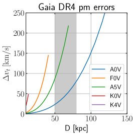
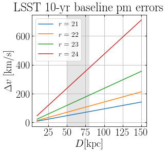
Figure 29: Top Panel: Accuracies in the tangential velocities as a function of Galactocentric distances for different stellar tracers for Gaia data release 4. Each colored solid line ends at the Gaia sensitivity limit. Beyond 50 kpc, A-type stars are the only observable stars in Gaia DR4 with errors in tangential velocities in the range of 50-100 km/s. These estimates where computed using the PyGaia library. Bottom Panel: LSST 10-year long baseline accuracies in the tangential velocities as a function of Galactocentric distances for different magnitudes. The shaded grey regions in both panels illustrates the regions of interest for our analysis. In those regions, LSST accuracies range from 30 up to 400 km/s for the faintest objects.

For LSST, the expected accuracies after a 10 yr long baseline will be similar to Gaia’s accuracies, but for fainter sources up to r$\sim$21, see Figure 21 in Ivezić et al. (2012) and Table 3 in Ivezić et al. (2008). LSST’s sensitivity will allow us to observe fainter objects with r$\sim$24. Figure 29 shows the accuracies in tangential velocities as a function of Galactocentric distances for different magnitudes. Between 50 and 80 kpc (our region of interest), LSST accuracies range from 30 km/s up to 400 km/s for the faintest objects $r=24$.

References

- Abadi et al. (2006) Abadi, M. G., Navarro, J. F., & Steinmetz, M. 2006, MNRAS, 365, 747, doi: 10.1111/j.1365-2966.2005.09789.x
- Astropy Collaboration et al. (2013) Astropy Collaboration, Robitaille, T. P., Tollerud, E. J., et al. 2013, aap, 558, A33, doi: 10.1051/0004-6361/201322068
- Behroozi et al. (2010) Behroozi, P. S., Conroy, C., & Wechsler, R. H. 2010, ApJ, 717, 379, doi: 10.1088/0004-637X/717/1/379
- Besla et al. (2013) Besla, G., Hernquist, L., & Loeb, A. 2013, MNRAS, 428, 2342, doi: 10.1093/mnras/sts192
- Besla et al. (2007) Besla, G., Kallivayalil, N., Hernquist, L., et al. 2007, ApJ, 668, 949, doi: 10.1086/521385
- Besla et al. (2010) —. 2010, ApJ, 721, L97, doi: 10.1088/2041-8205/721/2/L97
- Besla et al. (2012) —. 2012, MNRAS, 421, 2109, doi: 10.1111/j.1365-2966.2012.20466.x
- Besla et al. (2016) Besla, G., Martínez-Delgado, D., van der Marel, R. P., et al. 2016, ApJ, 825, 20, doi: 10.3847/0004-637X/825/1/20
- Besla et al. (2018) Besla, G., Patton, D. R., Stierwalt, S., et al. 2018, MNRAS, 480, 3376, doi: 10.1093/mnras/sty2041
- Binney & Tremaine (2008) Binney, J., & Tremaine, S. 2008, Galactic Dynamics: Second Edition (Princeton University Press)
- Boylan-Kolchin et al. (2011) Boylan-Kolchin, M., Besla, G., & Hernquist, L. 2011, MNRAS, 414, 1560, doi: 10.1111/j.1365-2966.2011.18495.x
- Bullock & Johnston (2005) Bullock, J. S., & Johnston, K. V. 2005, ApJ, 635, 931, doi: 10.1086/497422
- Buschmann et al. (2018) Buschmann, M., Kopp, J., Safdi, B. R., & Wu, C.-L. 2018, Phys. Rev. Lett., 120, 211101, doi: 10.1103/PhysRevLett.120.211101
- Busha et al. (2011) Busha, M. T., Marshall, P. J., Wechsler, R. H., Klypin, A., & Primack, J. 2011, ApJ, 743, 40, doi: 10.1088/0004-637X/743/1/40
- Carlin et al. (2016) Carlin, J. L., Liu, C., Newberg, H. J., et al. 2016, ApJ, 822, 16, doi: 10.3847/0004-637X/822/1/16
- Cautun et al. (2019) Cautun, M., Deason, A. J., Frenk, C. S., & McAlpine, S. 2019, MNRAS, 483, 2185, doi: 10.1093/mnras/sty3084
- Chandrasekhar (1943) Chandrasekhar, S. 1943, ApJ, 97, 255, doi: 10.1086/144517
- Choi et al. (2009) Choi, J.-H., Weinberg, M. D., & Katz, N. 2009, MNRAS, 400, 1247, doi: 10.1111/j.1365-2966.2009.15556.x
- Connors et al. (2006) Connors, T. W., Kawata, D., & Gibson, B. K. 2006, MNRAS, 371, 108, doi: 10.1111/j.1365-2966.2006.10659.x
- Cunningham et al. (2019) Cunningham, E. C., Deason, A. J., Sanderson, R. E., et al. 2019, ApJ, 879, 120, doi: 10.3847/1538-4357/ab24cd
- Deason et al. (2018) Deason, A. J., Belokurov, V., & Koposov, S. E. 2018, ApJ, 852, 118, doi: 10.3847/1538-4357/aa9d19
- Deason et al. (2014) Deason, A. J., Belokurov, V., Koposov, S. E., & Rockosi, C. M. 2014, ApJ, 787, 30, doi: 10.1088/0004-637X/787/1/30
- Dey et al. (2019) Dey, A., Najita, J. R., Koposov, S., et al. 2019, in BAAS, Vol. 51, 489
- Diaz & Bekki (2011) Diaz, J., & Bekki, K. 2011, MNRAS, 413, 2015, doi: 10.1111/j.1365-2966.2011.18289.x
- Diaz & Bekki (2012) Diaz, J. D., & Bekki, K. 2012, ApJ, 750, 36, doi: 10.1088/0004-637X/750/1/36
- Dierickx & Loeb (2017) Dierickx, M. I. P., & Loeb, A. 2017, ApJ, 836, 92, doi: 10.3847/1538-4357/836/1/92
- D’Onghia & Lake (2008) D’Onghia, E., & Lake, G. 2008, ApJ, 686, L61, doi: 10.1086/592995
- Eddington (1916) Eddington, A. S. 1916, MNRAS, 76, 572, doi: 10.1093/mnras/76.7.572
- Einasto (1965) Einasto, J. 1965, Trudy Astrofizicheskogo Instituta Alma-Ata, 5, 87
- Erkal et al. (2018) Erkal, D., Li, T. S., Koposov, S. E., et al. 2018, MNRAS, 481, 3148, doi: 10.1093/mnras/sty2518
- Erkal et al. (2019) Erkal, D., Belokurov, V., Laporte, C. F. P., et al. 2019, MNRAS, 487, 2685, doi: 10.1093/mnras/stz1371
- Fardal et al. (2019) Fardal, M. A., van der Marel, R. P., Law, D. R., et al. 2019, MNRAS, 483, 4724, doi: 10.1093/mnras/sty3428
- Furlanetto & Loeb (2002) Furlanetto, S. R., & Loeb, A. 2002, ApJ, 565, 854, doi: 10.1086/324693
- Gardiner & Noguchi (1996) Gardiner, L. T., & Noguchi, M. 1996, MNRAS, 278, 191, doi: 10.1093/mnras/278.1.191
- Gómez et al. (2015) Gómez, F. A., Besla, G., Carpintero, D. D., et al. 2015, ApJ, 802, 128, doi: 10.1088/0004-637X/802/2/128
- Gómez et al. (2010) Gómez, F. A., Helmi, A., Brown, A. G. A., & Li, Y.-S. 2010, MNRAS, 408, 935, doi: 10.1111/j.1365-2966.2010.17225.x
- Gómez et al. (2017) Gómez, F. A., White, S. D. M., Grand, R. J. J., et al. 2017, MNRAS, 465, 3446, doi: 10.1093/mnras/stw2957
- Gómez et al. (2016) Gómez, F. A., White, S. D. M., Marinacci, F., et al. 2016, MNRAS, 456, 2779, doi: 10.1093/mnras/stv2786
- González et al. (2013) González, R. E., Kravtsov, A. V., & Gnedin, N. Y. 2013, ApJ, 770, 96, doi: 10.1088/0004-637X/770/2/96
- Górski et al. (2005) Górski, K. M., Hivon, E., Banday, A. J., et al. 2005, ApJ, 622, 759, doi: 10.1086/427976
- Green (2002a) Green, A. M. 2002a, arXiv e-prints, hep. https://arxiv.org/abs/hep-ph/0208140
- Green (2002b) —. 2002b, Phys. Rev. D, 66, 083003, doi: 10.1103/PhysRevD.66.083003
- Guglielmo et al. (2014) Guglielmo, M., Lewis, G. F., & Bland-Hawthorn, J. 2014, MNRAS, 444, 1759, doi: 10.1093/mnras/stu1549
- Guo et al. (2010) Guo, Q., White, S., Li, C., & Boylan-Kolchin, M. 2010, MNRAS, 404, 1111, doi: 10.1111/j.1365-2966.2010.16341.x
- Hansen & Moore (2006) Hansen, S. H., & Moore, B. 2006, New A, 11, 333, doi: 10.1016/j.newast.2005.09.001
- Hashimoto et al. (2003) Hashimoto, Y., Funato, Y., & Makino, J. 2003, ApJ, 582, 196, doi: 10.1086/344260
- Helmi (2008) Helmi, A. 2008, A&A Rev., 15, 145, doi: 10.1007/s00159-008-0009-6
- Hernitschek et al. (2018) Hernitschek, N., Cohen, J. G., Rix, H.-W., et al. 2018, ApJ, 859, 31, doi: 10.3847/1538-4357/aabfbb
- Hernquist (1990) Hernquist, L. 1990, ApJ, 356, 359, doi: 10.1086/168845
- Hui et al. (2017) Hui, L., Ostriker, J. P., Tremaine, S., & Witten, E. 2017, Phys. Rev. D, 95, 043541, doi: 10.1103/PhysRevD.95.043541
- Hunter (2007) Hunter, J. D. 2007, Computing In Science & Engineering, 9, 90, doi: 10.1109/MCSE.2007.55
- Ivezić et al. (2012) Ivezić, Ž., Beers, T. C., & Jurić, M. 2012, ARA&A, 50, 251, doi: 10.1146/annurev-astro-081811-125504
- Ivezić et al. (2008) Ivezić, Ž., Kahn, S. M., Tyson, J. A., et al. 2008, ArXiv e-prints, arXiv:0805.2366. https://arxiv.org/abs/0805.2366
- Jethwa et al. (2016) Jethwa, P., Erkal, D., & Belokurov, V. 2016, MNRAS, 461, 2212, doi: 10.1093/mnras/stw1343
- Johnston et al. (2008) Johnston, K. V., Bullock, J. S., Sharma, S., et al. 2008, ApJ, 689, 936, doi: 10.1086/592228
- Jones et al. (2001–) Jones, E., Oliphant, T., Peterson, P., et al. 2001–, SciPy: Open source scientific tools for Python. http://www.scipy.org/
- Kahn & Woltjer (1959) Kahn, F. D., & Woltjer, L. 1959, ApJ, 130, 705, doi: 10.1086/146762
- Kallivayalil et al. (2013) Kallivayalil, N., van der Marel, R. P., Besla, G., Anderson, J., & Alcock, C. 2013, ApJ, 764, 161, doi: 10.1088/0004-637X/764/2/161
- Kallivayalil et al. (2018) Kallivayalil, N., Sales, L. V., Zivick, P., et al. 2018, ApJ, 867, 19, doi: 10.3847/1538-4357/aadfee
- Kluyver et al. (2016) Kluyver, T., Ragan-Kelley, B., Pérez, F., et al. 2016, in Positioning and Power in Academic Publishing: Players, Agents and Agendas, ed. F. Loizides & B. Schmidt, IOS Press, 87 – 90
- Klypin et al. (2011) Klypin, A. A., Trujillo-Gomez, S., & Primack, J. 2011, ApJ, 740, 102, doi: 10.1088/0004-637X/740/2/102
- Kochanek (1996) Kochanek, C. S. 1996, ApJ, 457, 228, doi: 10.1086/176724
- Koposov et al. (2019) Koposov, S. E., Belokurov, V., Li, T. S., et al. 2019, MNRAS, 485, 4726, doi: 10.1093/mnras/stz457
- Laporte et al. (2016) Laporte, C. F. P., Gómez, F. A., Besla, G., Johnston, K. V., & Garavito-Camargo, N. 2016, ArXiv e-prints. https://arxiv.org/abs/1608.04743
- Laporte et al. (2018a) Laporte, C. F. P., Gómez, F. A., Besla, G., Johnston, K. V., & Garavito-Camargo, N. 2018a, MNRAS, 473, 1218, doi: 10.1093/mnras/stx2146
- Laporte et al. (2018b) Laporte, C. F. P., Johnston, K. V., Gómez, F. A., Garavito-Camargo, N., & Besla, G. 2018b, MNRAS, 1495, doi: 10.1093/mnras/sty1574
- Laporte et al. (2013a) Laporte, C. F. P., Walker, M. G., & Peñarrubia, J. 2013a, MNRAS, 433, L54, doi: 10.1093/mnrasl/slt057
- Laporte et al. (2013b) Laporte, C. F. P., White, S. D. M., Naab, T., & Gao, L. 2013b, MNRAS, 435, 901, doi: 10.1093/mnras/stt912
- Li et al. (2019) Li, T. S., Kaplinghat, M., Bechtol, K., et al. 2019, arXiv e-prints, arXiv:1903.03155. https://arxiv.org/abs/1903.03155
- Loebman et al. (2018) Loebman, S. R., Valluri, M., Hattori, K., et al. 2018, ApJ, 853, 196, doi: 10.3847/1538-4357/aaa0d6
- Lynden-Bell (1981) Lynden-Bell, D. 1981, The Observatory, 101, 111
- Mackey et al. (2016) Mackey, A. D., Koposov, S. E., Erkal, D., et al. 2016, MNRAS, 459, 239, doi: 10.1093/mnras/stw497
- Mastropietro et al. (2005) Mastropietro, C., Moore, B., Mayer, L., Wadsley, J., & Stadel, J. 2005, MNRAS, 363, 509, doi: 10.1111/j.1365-2966.2005.09435.x
- Mateu et al. (2018) Mateu, C., Read, J. I., & Kawata, D. 2018, MNRAS, 474, 4112, doi: 10.1093/mnras/stx2937
- McMillan (2017) McMillan, P. J. 2017, MNRAS, 465, 76, doi: 10.1093/mnras/stw2759
- Merritt et al. (2006) Merritt, D., Graham, A. W., Moore, B., Diemand, J., & Terzić, B. 2006, AJ, 132, 2685, doi: 10.1086/508988
- Moster et al. (2010) Moster, B. P., Somerville, R. S., Maulbetsch, C., et al. 2010, ApJ, 710, 903, doi: 10.1088/0004-637X/710/2/903
- Nidever et al. (2019) Nidever, D. L., Olsen, K., Choi, Y., et al. 2019, ApJ, 874, 118, doi: 10.3847/1538-4357/aafaf7
- Ogiya & Burkert (2016) Ogiya, G., & Burkert, A. 2016, MNRAS, 457, 2164, doi: 10.1093/mnras/stw091
- Pardy et al. (2018) Pardy, S. A., D’Onghia, E., & Fox, A. J. 2018, ApJ, 857, 101, doi: 10.3847/1538-4357/aab95b
- Partridge et al. (2013) Partridge, C., Lahav, O., & Hoffman, Y. 2013, MNRAS, 436, L45, doi: 10.1093/mnrasl/slt109
- Patel et al. (2017a) Patel, E., Besla, G., & Mandel, K. 2017a, MNRAS, 468, 3428, doi: 10.1093/mnras/stx698
- Patel et al. (2017b) Patel, E., Besla, G., & Sohn, S. T. 2017b, MNRAS, 464, 3825, doi: 10.1093/mnras/stw2616
- Peñarrubia et al. (2016) Peñarrubia, J., Gómez, F. A., Besla, G., Erkal, D., & Ma, Y.-Z. 2016, MNRAS, 456, L54, doi: 10.1093/mnrasl/slv160
- Peñarrubia et al. (2014) Peñarrubia, J., Ma, Y.-Z., Walker, M. G., & McConnachie, A. 2014, MNRAS, 443, 2204, doi: 10.1093/mnras/stu879
- Peñarrubia et al. (2008) Peñarrubia, J., McConnachie, A. W., & Navarro, J. F. 2008, ApJ, 672, 904, doi: 10.1086/521543
- Pedregosa et al. (2011) Pedregosa, F., Varoquaux, G., Gramfort, A., et al. 2011, Journal of Machine Learning Research, 12, 2825
- Peebles (2010) Peebles, P. J. E. 2010, ArXiv e-prints, arXiv:1009.0496. https://arxiv.org/abs/1009.0496
- Pérez & Granger (2007) Pérez, F., & Granger, B. E. 2007, Computing in Science and Engineering, 9, 21, doi: 10.1109/MCSE.2007.53
- Power et al. (2003) Power, C., Navarro, J. F., Jenkins, A., et al. 2003, MNRAS, 338, 14, doi: 10.1046/j.1365-8711.2003.05925.x
- Price-Whelan et al. (2018) Price-Whelan, A. M., Sip’ocz, B. M., G”unther, H. M., et al. 2018, aj, 156, 123, doi: 10.3847/1538-3881/aabc4f
- Rashkov et al. (2013) Rashkov, V., Pillepich, A., Deason, A. J., et al. 2013, ApJ, 773, L32, doi: 10.1088/2041-8205/773/2/L32
- Read et al. (2006) Read, J. I., Goerdt, T., Moore, B., et al. 2006, MNRAS, 373, 1451, doi: 10.1111/j.1365-2966.2006.11022.x
- Roediger & Brüggen (2006) Roediger, E., & Brüggen, M. 2006, MNRAS, 369, 567, doi: 10.1111/j.1365-2966.2006.10335.x
- Saha et al. (2010) Saha, A., Olszewski, E. W., Brondel, B., et al. 2010, AJ, 140, 1719, doi: 10.1088/0004-6256/140/6/1719
- Salem et al. (2015) Salem, M., Besla, G., Bryan, G., et al. 2015, ApJ, 815, 77, doi: 10.1088/0004-637X/815/1/77
- Sales et al. (2007) Sales, L. V., Navarro, J. F., Abadi, M. G., & Steinmetz, M. 2007, MNRAS, 379, 1464, doi: 10.1111/j.1365-2966.2007.12024.x
- Sales et al. (2011) Sales, L. V., Navarro, J. F., Cooper, A. P., et al. 2011, MNRAS, 418, 648, doi: 10.1111/j.1365-2966.2011.19514.x
- Sandage (1986) Sandage, A. 1986, ApJ, 307, 1, doi: 10.1086/164387
- Sanderson et al. (2019) Sanderson, R., Carlin, J., Cunningham, E., et al. 2019, in BAAS, Vol. 51, 347
- Shao et al. (2018) Shao, S., Cautun, M., Deason, A. J., Frenk, C. S., & Theuns, T. 2018, MNRAS, 479, 284, doi: 10.1093/mnras/sty1470
- Springel (2005) Springel, V. 2005, MNRAS, 364, 1105, doi: 10.1111/j.1365-2966.2005.09655.x
- Springel et al. (2008) Springel, V., Wang, J., Vogelsberger, M., et al. 2008, MNRAS, 391, 1685, doi: 10.1111/j.1365-2966.2008.14066.x
- Thompson (2014) Thompson, R. 2014, pyGadgetReader: GADGET snapshot reader for python, Astrophysics Source Code Library. http://ascl.net/1411.001
- Tremaine & Weinberg (1984) Tremaine, S., & Weinberg, M. D. 1984, MNRAS, 209, 729, doi: 10.1093/mnras/209.4.729
- van den Bosch & Ogiya (2018) van den Bosch, F. C., & Ogiya, G. 2018, MNRAS, 475, 4066, doi: 10.1093/mnras/sty084
- van den Bosch et al. (2018) van den Bosch, F. C., Ogiya, G., Hahn, O., & Burkert, A. 2018, MNRAS, 474, 3043, doi: 10.1093/mnras/stx2956
- van der Marel et al. (2012) van der Marel, R. P., Fardal, M., Besla, G., et al. 2012, ApJ, 753, 8, doi: 10.1088/0004-637X/753/1/8
- van der Marel & Kallivayalil (2014) van der Marel, R. P., & Kallivayalil, N. 2014, ApJ, 781, 121, doi: 10.1088/0004-637X/781/2/121
- van der Marel et al. (2009) van der Marel, R. P., Kallivayalil, N., & Besla, G. 2009, in IAU Symposium, Vol. 256, The Magellanic System: Stars, Gas, and Galaxies, ed. J. T. Van Loon & J. M. Oliveira, 81–92
- van der Walt et al. (2011) van der Walt, S., Colbert, S. C., & Varoquaux, G. 2011, Computing in Science and Engineering, 13, 22, doi: 10.1109/MCSE.2011.37
- Wang et al. (2018) Wang, W., Han, J., Cole, S., et al. 2018, MNRAS, 476, 5669, doi: 10.1093/mnras/sty706
- Watkins et al. (2010) Watkins, L. L., Evans, N. W., & An, J. H. 2010, MNRAS, 406, 264, doi: 10.1111/j.1365-2966.2010.16708.x
- Weinberg (1989) Weinberg, M. D. 1989, MNRAS, 239, 549, doi: 10.1093/mnras/239.2.549
- Weinberg (1995) —. 1995, ApJ, 455, L31, doi: 10.1086/309803
- Weinberg (1998a) —. 1998a, MNRAS, 299, 499, doi: 10.1046/j.1365-8711.1998.01790.x
- Weinberg (1998b) —. 1998b, MNRAS, 297, 101, doi: 10.1046/j.1365-8711.1998.01456.x
- Weinberg & Blitz (2006) Weinberg, M. D., & Blitz, L. 2006, ApJ, 641, L33, doi: 10.1086/503607
- Weinberg & Katz (2007) Weinberg, M. D., & Katz, N. 2007, MNRAS, 375, 425, doi: 10.1111/j.1365-2966.2006.11306.x
- Wetzel et al. (2016) Wetzel, A. R., Hopkins, P. F., Kim, J.-h., et al. 2016, ApJ, 827, L23, doi: 10.3847/2041-8205/827/2/L23
- White (1983) White, S. D. M. 1983, ApJ, 274, 53, doi: 10.1086/161425
- Xue et al. (2015) Xue, X.-X., Rix, H.-W., Ma, Z., et al. 2015, ApJ, 809, 144, doi: 10.1088/0004-637X/809/2/144
- Yoshizawa & Noguchi (2003) Yoshizawa, A. M., & Noguchi, M. 2003, MNRAS, 339, 1135, doi: 10.1046/j.1365-8711.2003.06263.x
- Yurin & Springel (2014) Yurin, D., & Springel, V. 2014, MNRAS, 444, 62, doi: 10.1093/mnras/stu1421