Feedback Stabilization of a Class of Diagonal Infinite-Dimensional Systems with Delay Boundary Control

Abstract

This paper studies the boundary feedback stabilization of a class of diagonal infinite-dimensional boundary control systems. In the studied setting, the boundary control input is subject to a constant delay while the open loop system might exhibit a finite number of unstable modes. The proposed control design strategy consists in two main steps. First, a finite-dimensional subsystem is obtained by truncation of the original Infinite-Dimensional System (IDS) via modal decomposition. It includes the unstable components of the infinite-dimensional system and allows the design of a finite-dimensional delay controller by means of the Artstein transformation and the pole-shifting theorem. Second, it is shown via the selection of an adequate Lyapunov function that 1) the finite-dimensional delay controller successfully stabilizes the original infinite-dimensional system ; 2) the closed-loop system is exponentially Input-to-State Stable (ISS) with respect to distributed disturbances. Finally, the obtained ISS property is used to derive a small gain condition ensuring the stability of an IDS-ODE interconnection.

I Introduction

Feedback control of finite-dimensional systems in the presence of input delays has been extensively investigated [1, 18]. The extension of this topic to Infinite-Dimensional Systems (IDS), and in particular to Partial Differential Equations (PDEs), has attracted much attention in the recent years.

There exist essentially two types of control inputs for infinite-dimensional systems: bounded and unbounded control operators. The stability of linear and semilinear infinite-dimensional system under time-varying delayed feedback acting via a bounded linear control operator has been studied, e.g., in [8, 20]. In this paper, we are interested in the second type of control, i.e., when the control input acts on the system via an unbounded operator. For PDEs, such a setting takes the form of a control acting in the boundary conditions.

Unbounded control operators have been considered in the stability study of various PDEs. The cases of the heat [15] and wave [13, 14, 15] equations were studied via Lyapunov methods for slow time vaying delays. The cases of a parabolic PDE and a second-order evolution equation were reported in [23] and [7], respectively. The extension to a delayed ODE–heat cascade under actuator saturation was reported in [9].

In this paper, we are interested in the boundary feedback stabilization of a class of diagonal infinite dimensional boundary control systems in the presence of a constant input delay. Specifically, we consider the case of a boundary control system [6] for which the associated disturbance free operator is a Riesz-spectral operator admitting a finite number of unstable eigenvalues. The control design objective consists in the feedback stabilization of the system by means of a delay boundary control.

One of the very first contributions on input delayed unstable PDEs deals with a reaction-diffusion equation [11] where the controller was designed by resorting to the backstepping technique. The approach adopted in this paper differs. It relies on the following three steps procedure initially reported in [19]: 1) obtaining a finite-dimensional subsystem capturing the unstable modes by truncation of the original infinite-dimensional via a modal decomposition ; 2) design of a finite dimensional control law that stabilizes the finite-dimensional unstable part of the system ; 3) use of an adequate Lyapunov function to assess that the designed control law stabilizes the original infinite-dimensional system. Such a control design strategy was successfully applied to the stabilization of semilinear heat [4] and wave [5] equations via (undelayed) boundary feedback control. The extension of this design procedure to the delay feedback control of a linear reaction-diffusion equation was reported in [17, 22]. The delayed finite dimensional model was obtained via spectral reduction. Then, the control law was computed by applying the Artstein transformation [1, 18] and by resorting to the classical pole-shifting theorem. A distinguished feature is that, under the knowledge of the constant delay $D\geq 0$, the obtained finite-dimensional control law amounts stabilizing the closed-loop system, whatever the value of the time-delay $D$ may be.

In this context, the contribution of the present paper is fourfold.

1. We generalize the approach developed in [17] for the delay feedback control of a linear reaction-diffusion equation with one-dimensional control input to the general case of the delay boundary feedback stabilization of a class of diagonal infinite dimensional boundary control systems with finitely many unstable modes and finite dimensional input. The control design strategy relies on the design of the feedback control law based on a finite-dimensional truncated part of the original system. The truncation is performed via a spectral decomposition used to capture the unstable modes of the system. The control law is then obtained based on this finite-dimensional subsystem with delay control input by means of the Artstein transformation and the pole-shifting theorem. The exponential stability of the resulting closed-loop infinite dimensional system is assessed via the introduction of a suitable Lyapunov function.

2. In [4, 5, 17] the control design was performed on the time derivative $v=\dot{u}$ of the actual input signal $u$. Thus, the application of the control law required an a posteriori integration of $v$ to obtain the actual control input $u$. In this paper, we propose a simplification of the control law that avoids such an a posteriori integration. Such a simplification is allowed by an adequate spectral decomposition that only involves the value of the control input while avoiding the occurrence of its time derivative.

3. We show that the resulting closed-loop system is exponentially Input-to-State Stable (ISS)[21] with respect to distributed disturbances acting via a bounded operator.

4. Taking advantage of the ISS property of the closed-loop infinite-dimensional system, we derive a small gain condition ensuring the stability of an IDS-ODE interconnection. We follow here the methodology presented in [10] that relies on the conversion of the ISS estimates satisfied by each component of the interconnection into fading memory estimates[10, Lemma 7.1]. However, such a conversion does not apply to the studied closed-loop infinite-dimensional system due to the time-varying nature of the control strategy. This pitfall is avoided by working directly with the Lyapunov function instead of the trajectories of the system.

The remainder of this paper is organized as follows. Both problem setting and control objectives are introduced in Section II. The comprehensive construction of the control strategy is presented in Section III. It consists first in the spectral decomposition of the problem in order to obtain a finite-dimensional model capturing the unstable modes (Subsection III-A) and then the design of the finite dimensional controller stabilizing the obtained truncated subsystem. The study of the ISS property of the resulting closed-loop infinite-dimensional system is carried out via the introduction of an adequate Lyapunov function in Section IV. We take advantage of these results to derive in Section V a small gain condition ensuring the stability of an IDS-ODE interconnection. In Section VI, we check the assumptions on a IDS-ODE system and in particular the small gain condition. The obtained numerical results are compliant with the theoretical predictions. Finally, concluding remarks are provided in Section VII.

II Problem setting and control objective

Throughout the paper, we assume that $(\mathcal{H},\left<\cdot,\cdot\right>_{\mathcal{H}})$ is a separable Hilbert space over the field $\mathbb{K}$, which is either $\mathbb{R}$ or $\mathbb{C}$. All the finite-dimensional spaces $\mathbb{K}^{p}$ are endowed with the usual euclidean inner product $\left<x,y\right>=x^{*}y$ and the associated 2-norm $\|x\|=\sqrt{\left<x,x\right>}=\sqrt{x^{*}x}$, where $x^{*}=\overline{x}^{\top}$. For any matrix $M\in\mathbb{K}^{p\times q}$, $\|M\|$ stands for the induced norm of $M$ associated with the above 2-norms.

II-A Problem setting

We consider the abstract boundary control systems [6] with delayed boundary control

$$\left\{\begin{split}\dfrac{\mathrm{d}X}{\mathrm{d}t}(t)&=\mathcal{A}X(t)+d(t),&t\geq 0\\ \mathcal{B}X(t)&=u_{D}(t)\triangleq u(t-D),&t\geq 0\\ X(0)&=X_{0}\end{split}\right.$$ (1)

with

• $\mathcal{A}:D(\mathcal{A})\subset\mathcal{H}\rightarrow\mathcal{H}$ a linear (unbounded) operator;

• $\mathcal{B}:D(\mathcal{B})\subset\mathcal{H}\rightarrow\mathbb{K}^{m}$ with $D(\mathcal{A})\subset D(\mathcal{B})$ a linear boundary operator;

• $d:\mathbb{R}_{+}\rightarrow\mathcal{H}$ a distributed disturbance;

• $u:[-D,+\infty)\rightarrow\mathbb{K}^{m}$, with a known constant delay $D>0$ and $\left.u\right|_{[-D,0)}=0$, the boundary control.

We assume that $(\mathcal{A},\mathcal{B})$ is a boundary control system, i.e.,

1. the disturbance free operator $\mathcal{A}_{0}$, defined over the domain $D(\mathcal{A}_{0})\triangleq D(\mathcal{A})\cap\mathrm{ker}(\mathcal{B})$ by $\mathcal{A}_{0}\triangleq\left.\mathcal{A}\right|_{D(\mathcal{A}_{0})}$, is the generator of a $C_{0}$-semigroup $S$ on $\mathcal{H}$;

2. there exists a bounded operator $B\in\mathcal{L}(\mathbb{K}^{m},\mathcal{H})$, called a lifting operator, such that $\mathrm{R}(B)\subset D(\mathcal{A})$, $\mathcal{A}B\in\mathcal{L}(\mathbb{K}^{m},\mathcal{H})$, and $\mathcal{B}B=I_{\mathbb{K}^{m}}$.

It is recalled that $\mathrm{ker}(\mathcal{B})$ is the kernel of $\mathcal{B}$ while $\mathrm{R}(B)$ stands for the range of $B$. We make the following assumptions.

Assumption II.1

The disturbance free operator $\mathcal{A}_{0}$ is a Riesz spectral operator [6], i.e., is a linear and closed operator with simple eigenvalues $\lambda_{n}$ and corresponding eigenvectors $\phi_{n}\in D(\mathcal{A}_{0})$, $n\in\mathbb{N}^{*}$, that satisfy:

1. $\left\{\phi_{n},\;n\in\mathbb{N}^{*}\right\}$ is a Riesz basis [3]:

   1. $\overline{\underset{n\in\mathbb{N}^{*}}{\mathrm{span}_{\mathbb{K}}}\;\phi_{n}}=\mathcal{H}$;

   2. there exist constants $m_{R},M_{R}\in\mathbb{R}_{+}^{*}$ such that for all $N\in\mathbb{N}^{*}$ and all $\alpha_{1},\ldots,\alpha_{N}\in\mathbb{K}$,

      $$m_{R}\sum\limits_{n=1}^{N}|\alpha_{n}|^{2}\leq\left\|\sum\limits_{n=1}^{N}\alpha_{n}\phi_{n}\right\|_{\mathcal{H}}^{2}\leq M_{R}\sum\limits_{n=1}^{N}|\alpha_{n}|^{2}.$$ (2)

2. The closure of $\{\lambda_{n},\;n\in\mathbb{N}^{*}\}$ is totally disconnected, i.e. for any distinct $a,b\in\overline{\{\lambda_{n},\;n\in\mathbb{N}^{*}\}}$, $[a,b]\not\subset\overline{\{\lambda_{n},\;n\in\mathbb{N}^{*}\}}$.

Assumption II.2

There exist $N_{0}\in\mathbb{N}^{*}$ and $\alpha\in\mathbb{R}_{+}^{*}$ such that $\operatorname{Re}\lambda_{n}\leq-\alpha$ for all $n\geq N_{0}+1$.

Remark II.3

Note that Assumption II.2 is equivalent to:

• the number of unstable eigenvalues is finite, i.e., $\mathrm{Card}(\{\lambda_{n}\,:\,\operatorname{Re}\lambda_{n}\geq 0\})<\infty$ ;

• the set composed of the real part of the stable eigenvalues is not accumulating at 0, i.e., $\sup\limits_{\operatorname{Re}\lambda_{n}<0}\operatorname{Re}\lambda_{n}<0$.

From the well-known properties of the Riesz-basis (see, e.g., [3]), we introduce $\left\{\psi_{n},\;n\in\mathbb{N}^{*}\right\}$ the biorthogonal sequence associated with the Riesz basis $\left\{\phi_{n},\;n\in\mathbb{N}^{*}\right\}$, i.e., $\left<\phi_{k},\psi_{l}\right>_{\mathcal{H}}=\delta_{k,l}$. Then, the following series expansion holds true.

$$\forall x\in\mathcal{H},\qquad x=\sum\limits_{n\geq 1}\left<x,\psi_{n}\right>_{\mathcal{H}}\phi_{n}.$$

Furthermore, as $\mathcal{A}_{0}$ is assumed to be a Riesz-spectral operator, then $\psi_{n}$ is an eigenvector of the adjoint operator $\mathcal{A}_{0}^{*}$ associated with the eigenvalue $\overline{\lambda_{n}}$.

II-B Control objective

The control objective is twofold. First, in the absence of distributed disturbance (i.e., $d=0$), the control objective is to design a control law $u$ that exponentially stabilizes (if at least one eigenvalue has a non negative real part) and modify the pole placement associated with $\lambda_{1},\ldots,\lambda_{N_{0}}$ for (1). Second, the control law must ensure the ISS property of the closed-loop system with respect to the distributed disturbance $d$.

Because we are only concerned in controlling the system from the starting time $t=0$, we assume that the system is uncontrolled for $t<0$. This is why it is imposed $\left.u\right|_{[-D,0)}=0$. Therefore, due to the delay $D$ in the control input of (1), the system remains open-loop for $t<D$ while the effect of the control input will have an impact on the system only at times $t\geq D$.

Note that the $N_{0}\in\mathbb{N}^{*}$ and $\alpha>0$ provided by Assumption II.2 are not unique. For instance, one could select $N_{0}\in\mathbb{N}^{*}$ such that $\lambda_{1},\ldots,\lambda_{N_{0}}$ are all with non negative real part. In this case, the control design reduces to stabilize the unstable part of the system. Nevertheless, one could also want to improve the decay rate or the damping of certain of the stable open-loop eigenvalues. In this case, $\lambda_{1},\ldots,\lambda_{N_{0}}$ would include all the unstable eigenvalues and certain selected stable eigenvalues of the open-loop system.

III Construction of the feedback control strategy

In order to derive the control law, we make in this section the a priori assumption that $u\in\mathcal{C}^{2}([-D,+\infty);\mathbb{K}^{m})$. This assumption is necessary to ensure the existence of classical solutions of (1), and thus to proceed to the upcoming computations (see, e.g., [6]). Therefore, the construction of the control law must ensure that such a regularity property holds true. This will be assessed in the next section.

III-A Spectral decomposition

Assuming that $u_{D}\in\mathcal{C}^{2}([0,+\infty);\mathbb{K}^{m})$, $X_{0}\in D(\mathcal{A})$ such that $\mathcal{B}X_{0}=u_{D}(0)=0$ (i.e., $X_{0}\in D(\mathcal{A}_{0})$), and $d\in\mathcal{C}^{1}(\mathbb{R}_{+};\mathcal{H})$, we denote by $X\in\mathcal{C}^{0}(\mathbb{R}_{+};D(\mathcal{A}))\cap\mathcal{C}^{1}(\mathbb{R}_{+};\mathcal{H})$ the unique classical solution of (1). Then, we introduce $c_{n}(t)\triangleq\left<X(t),\psi_{n}\right>_{\mathcal{H}}$ the projection of $X(t)$ into the Riezs basis $\left\{\phi_{n},\;n\in\mathbb{N}^{*}\right\}$, i.e. (see [3]),

$$X(t)=\sum\limits_{n\in\mathbb{N}^{*}}\left<X(t),\psi_{n}\right>_{\mathcal{H}}\phi_{n}=\sum\limits_{n\in\mathbb{N}^{*}}c_{n}(t)\phi_{n}.$$ (3)

We also introduce $d_{n}(t)\triangleq\left<d(t),\psi_{n}\right>_{\mathcal{H}}$. Then $c_{n}\in\mathcal{C}^{1}(\mathbb{R}_{+};\mathbb{K})$ and, following [12], we infer from (1) that, for all $t\geq 0$,

$$\dot{c}_{n}(t)$$

$$=\left<\dfrac{\mathrm{d}X}{\mathrm{d}t}(t),\psi_{n}\right>_{\mathcal{H}}$$

$$=\left<\mathcal{A}X(t),\psi_{n}\right>_{\mathcal{H}}+\left<d(t),\psi_{n}\right>_{\mathcal{H}}$$

$$=\left<\mathcal{A}\left\{X(t)-Bu_{D}(t)\right\},\psi_{n}\right>_{\mathcal{H}}+\left<\mathcal{A}Bu_{D}(t),\psi_{n}\right>_{\mathcal{H}}+d_{n}(t)$$

$$=\left<\mathcal{A}_{0}\left\{X(t)-Bu_{D}(t)\right\},\psi_{n}\right>_{\mathcal{H}}+\left<\mathcal{A}Bu_{D}(t),\psi_{n}\right>_{\mathcal{H}}+d_{n}(t)$$

$$=\left<X(t)-Bu_{D}(t),\mathcal{A}_{0}^{*}\psi_{n}\right>_{\mathcal{H}}+\left<\mathcal{A}Bu_{D}(t),\psi_{n}\right>_{\mathcal{H}}+d_{n}(t)$$

$$=\left<X(t)-Bu_{D}(t),\overline{\lambda_{n}}\psi_{n}\right>_{\mathcal{H}}+\left<\mathcal{A}Bu_{D}(t),\psi_{n}\right>_{\mathcal{H}}+d_{n}(t)$$

$$=\lambda_{n}c_{n}(t)-\lambda_{n}\left<Bu_{D}(t),\psi_{n}\right>_{\mathcal{H}}+\left<\mathcal{A}Bu_{D}(t),\psi_{n}\right>_{\mathcal{H}}+d_{n}(t),$$ (4)

where it has been used that $\mathcal{B}\left\{X(t)-Bu_{D}(t)\right\}=u_{D}(t)-u_{D}(t)=0$, showing that $X(t)-Bu_{D}(t)\in D(\mathcal{A})\cap\mathrm{ker}(\mathcal{B})=D(\mathcal{A}_{0})$.

Remark III.1

It is interesting to note that the ODE (4) describing the time evolution of the coefficient $c_{n}(t)=\left<X(t),\psi_{n}\right>_{\mathcal{H}}$ only involves the delayed control input $u_{D}(t)$ while avoiding the occurrence of its time derivative $\dot{u}_{D}(t)$. Therefore, whereas it was necessary in [4, 5, 17], due to the presence of the term $\dot{u}_{D}(t)$ in the ODEs resulting from the spectral decomposition, to augment the state of the finite-dimensional subsystem and to use $\dot{u}_{D}(t)$ as a control input, we avoid here such a procedure. This yields a simplification of the control law by avoiding an a posteriori integration of $\dot{u}$ to obtain the actual control law $u$.

Let $\mathcal{E}=(e_{1},e_{2},\ldots,e_{m})$ be the canonical basis of $\mathbb{K}^{m}$, and consider the projections $u_{1},u_{2},\ldots,u_{m}\in\mathcal{C}^{2}([-D,+\infty);\mathbb{K})$ such that

$$u=\sum\limits_{k=1}^{m}u_{k}e_{k}=\begin{bmatrix}u_{1}\\ \vdots\\ u_{m}\end{bmatrix}.$$

Introducing $b_{n,k}\triangleq-\lambda_{n}\left<Be_{k},\psi_{n}\right>_{\mathcal{H}}+\left<\mathcal{A}Be_{k},\psi_{n}\right>_{\mathcal{H}}$, we obtain from (4) that

$$\dot{c}_{n}(t) =\lambda_{n}c_{n}(t)+\sum\limits_{k=1}^{m}b_{n,k}u_{D,k}(t)+\left<d(t),\psi_{n}\right>_{\mathcal{H}}.$$

Then, the following linear ODE with delay input holds true for all $t\geq 0$

$$\dot{Y}(t)=A_{N_{0}}Y(t)+B_{N_{0}}u_{D}(t)+D_{N_{0}}(t),$$ (5)

where $A_{N_{0}}=\mathrm{diag}(\lambda_{1},\ldots,\lambda_{N_{0}})\in\mathbb{K}^{N_{0}\times N_{0}}$, $B_{N_{0}}=(b_{n,k})_{1\leq n\leq N_{0},1\leq k\leq m}\in\mathbb{K}^{N_{0}\times m}$,

$$Y(t)=\begin{bmatrix}c_{1}(t)\\ \vdots\\ c_{N_{0}}(t)\end{bmatrix}=\begin{bmatrix}\left<X(t),\psi_{1}\right>_{\mathcal{H}}\\ \vdots\\ \left<X(t),\psi_{N_{0}}\right>_{\mathcal{H}}\end{bmatrix}\in\mathbb{K}^{N_{0}},$$

and

$$D_{N_{0}}(t)=\begin{bmatrix}d_{1}(t)\\ \vdots\\ d_{N_{0}}(t)\end{bmatrix}=\begin{bmatrix}\left<d(t),\psi_{1}\right>_{\mathcal{H}}\\ \vdots\\ \left<d(t),\psi_{N_{0}}\right>_{\mathcal{H}}\end{bmatrix}\in\mathbb{K}^{N_{0}}.$$ (6)

Note that the norm of $D_{N_{0}}(t)$ can be bounded above in function of the norm of the full distributed disturbance $d(t)$ as follows. For all $t\geq 0$, we have

$$\|D_{N_{0}}(t)\|^{2}=\sum\limits_{k=1}^{N_{0}}|\left<d(t),\psi_{k}\right>_{\mathcal{H}}|^{2} \leq\sum\limits_{k\geq 1}|\left<d(t),\psi_{k}\right>_{\mathcal{H}}|^{2}$$

$$\overset{(\ref{eq: Riesz basis - inequality})}{\leq}\dfrac{1}{m_{R}}\|d(t)\|_{\mathcal{H}}^{2}.$$ (7)

The finite-dimensional linear ODE (5) captures the part of the dynamics of (1) that must me stabilized/controlled by the feedback control $u$. The idea consists in first designing a control law that exponentially stabilizes the linear ODE (5). Then, we assess that the proposed control law amounts stabilizing the original infinite-dimensional system (1) by means of an adequate Lyapunov function.

III-B Stabilization of the finite-dimensional subsystem

At this point, we need to design a control law that stabilizes the linear ODE with input delay (5). First, we resort to the Artstein model reduction [1, 18] to obtain an equivalent linear ODE that is free of delay. Specifically, we introduce for all $t\geq 0$,

$$Z(t) =Y(t)+\int_{t-D}^{t}e^{(t-s-D)A_{N_{0}}}B_{N_{0}}u(s)\mathop{}\!\mathrm{d}s$$

$$=Y(t)+\int_{0}^{D}e^{-\tau A_{N_{0}}}B_{N_{0}}u(t-D+\tau)\mathop{}\!\mathrm{d}\tau.$$

Straightforward computations show that we have for all $t\geq 0$,

$$\dot{Z}(t)=A_{N_{0}}Z(t)+e^{-DA_{N_{0}}}B_{N_{0}}u(t)+D_{N_{0}}(t).$$

As $e^{-DA_{N_{0}}}$ is invertible and commutes with $A_{N_{0}}$, the pair $(A_{N_{0}},e^{-DA_{N_{0}}}B_{N_{0}})$ satisfies the Kalman condition if and only if the pair $(A_{N_{0}},B_{N_{0}})$ satisfies the Kalman condition. Consequently, in order to be able to apply the pole-shifting theorem, we make the following assumption.

Assumption III.2

$(A_{N_{0}},B_{N_{0}})$ satisfies the Kalman condition.

Remark III.3

In the case of a one-dimensional control input, i.e., $m=1$, we have that

$$\mathrm{det}(B_{N_{0}},A_{N_{0}}B_{N_{0}},\ldots,A_{N_{0}}^{N_{0}-1}B_{N_{0}})$$

$$\qquad=\prod\limits_{n=1}^{N_{0}}b_{n,1}\times\mathrm{VdM}(\lambda_{1},\ldots,\lambda_{N_{0}}),$$

where $\mathrm{VdM}(\lambda_{1},\ldots,\lambda_{N_{0}})$ is the Van der Monde determinant associated with $\lambda_{1},\ldots,\lambda_{N_{0}}$. Therefore Assumption III.2 is fulfilled if and only if $\lambda_{1},\ldots,\lambda_{N_{0}}$ are all distinct and $b_{n,1}\neq 0$ for all $1\leq n\leq N_{0}$. In the general case $m\geq 1$, we can easily apply the PBH test [24] due to the diagonal nature of the matrix $A_{N_{0}}$. Assume without loss of generality that $\lambda_{1},\ldots,\lambda_{N_{0}}$ are ordered such that there exist $n_{1},\ldots,n_{p}\in\mathbb{N}^{*}$ with $n_{1}+\ldots+n_{p}=N_{0}$ such that 1) for all $1\leq l\leq p$, $\lambda_{s_{l-1}+1}=\lambda_{s_{l-1}+2}=\ldots=\lambda_{s_{l}}$ ; 2) $l_{1}\neq l_{2}$ implies $\lambda_{s_{l_{1}}}\neq\lambda_{s_{l_{2}}}$, where $s_{l}=n_{1}+n_{2}+\ldots+n_{l}$. Then, Assumption III.2 is fulfilled if and only if $\mathrm{rank}[(b_{n,k})_{s_{l-1}+1\leq n\leq s_{l},1\leq k\leq m}]=n_{l}$. In particular, it requires the necessary condition that $n_{l}\leq m$ for all $1\leq l\leq p$.

Remark III.4

Note that $b_{n,k}$ is computed based on the selection of a given lifting operator $B$. Even if such a lifting operator is not unique, the quantity $b_{n,k}$ is actually independent of the particularly selected lifting operator. Indeed, let $B$ and $\tilde{B}$ be two distinct lifting operators associated with $(\mathcal{A},\mathcal{B})$. Then, introducing $\hat{B}=B-\tilde{B}$, one has $\mathcal{B}\hat{B}=\mathcal{B}B-\mathcal{B}\tilde{B}=I_{\mathbb{K}^{m}}-I_{\mathbb{K}^{m}}=0$. Thus, $R(\hat{B})\subset D(\mathcal{A})\cap\mathrm{ker}(\mathcal{B})=D(\mathcal{A}_{0})$ and we obtain that

$$\left<\mathcal{A}\hat{B}e_{k},\psi_{n}\right>_{\mathcal{H}} =\left<\mathcal{A}_{0}\hat{B}e_{k},\psi_{n}\right>_{\mathcal{H}}=\left<\hat{B}e_{k},\mathcal{A}_{0}^{*}\psi_{n}\right>_{\mathcal{H}}$$

$$=\left<\hat{B}e_{k},\overline{\lambda_{n}}\psi_{n}\right>_{\mathcal{H}}=\lambda_{n}\left<\hat{B}e_{k},\psi_{n}\right>_{\mathcal{H}}.$$

We deduce the claimed result, i.e.,

$$-\lambda_{n}\left<Be_{k},\psi_{n}\right>_{\mathcal{H}}+\left<\mathcal{A}Be_{k},\psi_{n}\right>_{\mathcal{H}}$$

$$\hskip 28.45274pt=-\lambda_{n}\left<\tilde{B}e_{k},\psi_{n}\right>_{\mathcal{H}}+\left<\mathcal{A}\tilde{B}e_{k},\psi_{n}\right>_{\mathcal{H}}.$$

Therefore, the commandability property of the pair $(A_{N_{0}},B_{N_{0}})$ is an intrinsic property of the boundary control system $(\mathcal{A},\mathcal{B})$ in the sense that it does not depend on the selection of a particular lifting operator $B$.

Assuming that Assumption III.2 holds true, we can find a feedback gain $K\in\mathbb{K}^{m\times N_{0}}$ and $P\in\mathcal{H}_{N_{0}}^{+*}$ Hermitian definite positive such that $A_{\mathrm{cl}}\triangleq A_{N_{0}}+e^{-DA_{N_{0}}}B_{N_{0}}K$ is Hurwitz with desired pole placement and

$$A_{\mathrm{cl}}^{*}P+PA_{\mathrm{cl}}=-I_{N_{0}}.$$

Then, a natural choice for the control input would be $u(t)=\chi_{[0,+\infty)}(t)KZ(t)$. However, the resulting $u_{D}(t)=u(t-D)=\chi_{[D,+\infty)}(t)KZ(t-D)$ is discontinuous at $t=D$ while $u_{D}$ must be of class $\mathcal{C}^{2}$ over $\mathbb{R}_{+}$ to ensure the existence of a classical solution of (1). Let $t_{0}>0$ be given. We consider a transition signal (from open loop to closed loop) $\varphi\in\mathcal{C}^{2}([-D,+\infty);\mathbb{R})$ which is such that $0\leq\varphi\leq 1$, $\left.\varphi\right|_{[-D,0]}=0$, and $\left.\varphi\right|_{[t_{0},+\infty)}=1$. We define the control input $u(t)=\varphi(t)KZ(t)$. It satisfies $\left.u\right|_{[-D,0]}=0$ and, for all $t\geq 0$,

$$u(t) =\varphi(t)KZ(t)$$

$$=\varphi(t)KY(t)$$ (8)

$$\phantom{=}\,+\varphi(t)K\int_{\max(t-D,0)}^{t}e^{(t-s-D)A_{N_{0}}}B_{N_{0}}u(s)\mathop{}\!\mathrm{d}s,$$

where it has been used that the system is uncontrolled for $t\leq 0$. In particular, the control law is such that $u_{D}(t)=u(t-D)=\varphi(t-D)KZ(t-D)$ with $u_{D}(t)=0$ for $t\leq D$ and $u_{D}(t)=KZ(t-D)$ for $t\geq D+t_{0}$.

III-C Characterization of the control law

In practice, it is convenient to use the control law expressed under the form (8) since it allows its computation at time $t$ based on the measure of $Y$ at time $t$ and the past history of the control law $u$. To do so, we must show that (8) fully characterizes $u$, i.e., the uniqueness of the function $u$ satisfying the implicit equation (8). In other words, it requires to invert the Artstein transformation [2] when weighted by the transition signal $\varphi$. For any locally integrable function $f:\mathbb{R}_{+}\rightarrow\mathbb{K}^{m}$, we define $T_{D}f:\mathbb{R}_{+}\rightarrow\mathbb{K}^{m}$ as follows:

$$(T_{D}f)(t)=\varphi(t)K\int_{\max(t-D,0)}^{t}e^{(t-s-D)A_{N_{0}}}B_{N_{0}}f(s)\mathop{}\!\mathrm{d}s.$$

In particular $T_{D}f\in\mathcal{C}^{0}(\mathbb{R}_{+};\mathbb{K}^{m})$, and thus we can consider the iterations $T_{D}^{n}f$ for any $n\in\mathbb{N}$.

Lemma III.5

Let $D>0$, $T\in\mathbb{R}_{+}^{*}\cup\{+\infty\}$, $g\in\mathcal{C}^{0}([0,T];\mathbb{K}^{N_{0}})$, and $\varphi\in\mathcal{C}^{0}([0,T];\mathbb{R})$ such that $0\leq\varphi\leq 1$ be given. Then, there exists a unique locally integrable function $v$ defined over $[0,T]$ such that for all $t\in[0,T]$,

$$v(t) =\varphi(t)Kg(t)$$

$$\phantom{=}\,+\varphi(t)K\int_{\max(t-D,0)}^{t}e^{(t-s-D)A_{N_{0}}}B_{N_{0}}v(s)\mathop{}\!\mathrm{d}s.$$

Furthermore $v\in\mathcal{C}^{0}([0,T];\mathbb{K}^{m})$ and is given by the following series expansion:

$$v(t)=\sum\limits_{k=0}^{\infty}(T_{D}^{k}(\varphi Kg))(t),$$

where the series converge uniformingly over any time interval of finite length.

The inversion of the Artstein transformation corresponding to the case $\varphi=1$ has been investigated in [2]. The proof of Lemma III.5 is a straightfoward extension of the proof of Theorem 1 in [2] by noting that $v=\varphi Kg+T_{D}v$ and by using the fact that $\varphi$ is a continuous function that satisfies $0\leq\varphi\leq 1$.

IV Study of the closed-loop infinite-dimensional system

Throughout this section, we assume that Assumptions II.1, II.2, and III.2 hold true. Under these conditions, it has been proposed in Section III to resort to the control law given by (8) to stabilize the infinite-dimensional system (1). As the control law has been derived on a finite-dimensional part of the original infinite-dimensional system, we must guarantee that the proposed control strategy successfully stabilizes the full system. Furthermore, in order to make valid the computations performed in the previous section, we must ensure that the a priori assumption is indeed satisfied, i.e., the proposed control law is of class $\mathcal{C}^{2}$.

IV-A Dynamics of the closed-loop system

Let $D,t_{0}>0$ be given. We consider a given transition signal $\varphi\in\mathcal{C}^{2}([-D,+\infty);\mathbb{R})$ such that $0\leq\varphi\leq 1$, $\left.\varphi\right|_{[-D,0]}=0$, and $\left.\varphi\right|_{[t_{0},+\infty)}=1$. The closed-loop system dynamics takes the following form:

$$\left\{\begin{split}\dfrac{\mathrm{d}X}{\mathrm{d}t}(t)&=\mathcal{A}X(t)+d(t),\\ \mathcal{B}X(t)&=u_{D}(t)=u(t-D),\\ \left.u\right|_{[-D,0]}&=0\\ u(t)&=\varphi(t)KY(t)\\ &\phantom{=}+\varphi(t)K\int_{\max(t-D,0)}^{t}e^{(t-s-D)A_{N_{0}}}B_{N_{0}}u(s)\mathop{}\!\mathrm{d}s,\\ Y(t)&=\begin{bmatrix}\left<X(t),\psi_{1}\right>_{\mathcal{H}}\\ \vdots\\ \left<X(t),\psi_{N_{0}}\right>_{\mathcal{H}}\end{bmatrix},\\ X(0)&=X_{0}\end{split}\right.$$ (9)

for any $t\geq 0$. The feedback gain $K\in\mathbb{K}^{m\times N_{0}}$ is such that $A_{\mathrm{cl}}\triangleq A_{N_{0}}+e^{-DA_{N_{0}}}B_{N_{0}}K$ is Hurwitz (with desired pole placement). Function $d:\mathbb{R}_{+}\rightarrow\mathcal{H}$ represents a distributed disturbance.

IV-B Well-posedness in terms of classical solutions

The following lemma ensures both the well-posedness of the closed-loop system in terms of classical solutions and the sufficient regularity of the control input.

Lemma IV.1

Let $(\mathcal{A},\mathcal{B})$ be an abstract boundary control system such that Assumptions II.1, II.2, and III.2 hold true. For any $X_{0}\in D(\mathcal{A}_{0})$ and $d\in\mathcal{C}^{1}(\mathbb{R}_{+};\mathcal{H})$, the closed-loop system (9) admits a unique classical solution $X\in\mathcal{C}^{0}(\mathbb{R}_{+};D(\mathcal{A}))\cap\mathcal{C}^{1}(\mathbb{R}_{+};\mathcal{H})$. The associated control law $u$ is uniquely defined and is of class $\mathcal{C}^{2}([-D,+\infty);\mathbb{K}^{m})$. It can be written under the form $u=\varphi KZ$ with, for all $t\geq 0$,

$$Z(t)\triangleq Y(t)+\int_{t-D}^{t}e^{(t-s-D)A_{N_{0}}}B_{N_{0}}u(s)\mathop{}\!\mathrm{d}s,$$ (10)

which is such that $Z\in\mathcal{C}^{2}(\mathbb{R}_{+};\mathbb{K}^{N_{0}})$ and satisfies, for all $t\geq 0$,

$$\dot{Z}(t)=(A_{N_{0}}+\varphi(t)e^{-DA_{N_{0}}}B_{N_{0}}K)Z(t)+D_{N_{0}}(t),$$ (11)

where $D_{N_{0}}(t)$ is defined by (6). In particular, for all $t\geq D+t_{0}$,

$$\dot{Z}(t)=A_{\mathrm{cl}}Z(t)+D_{N_{0}}(t).$$ (12)

Furthermore, $u$ is also expressed for all $t\geq 0$ by the following series expansion

$$u(t)=\sum\limits_{k=0}^{\infty}(T_{D}^{k}(\varphi KY))(t),$$ (13)

where the series converges uniformingly over any time interval of finite length.

Proof. We first note that, as $\left.u\right|_{[-D,0]}=0$, (9) is equivalent over the time interval $[0,D]$ to the following standard evolution problem

$$\left\{\begin{split}\dfrac{\mathrm{d}X}{\mathrm{d}t}(t)&=\mathcal{A}_{0}X(t)+d(t),&t\in[0,D]\\ X(0)&=X_{0}\end{split}\right.$$

As $\mathcal{A}_{0}$ generates a $C_{0}$-semigroup, we deduce (see, e.g., [6]) the existence and the uniqueness of a classical solution $X\in\mathcal{C}^{0}([0,D];D(\mathcal{A}))\cap\mathcal{C}^{1}([0,D];\mathcal{H})$ such that (9) holds true over the time interval $[0,D]$.

We now proceed by induction. Assume that, for a given $n\in\mathbb{N}^{*}$, there exists a unique classical solution over the time interval $[0,nD]$ denoted by $X\in\mathcal{C}^{0}([0,nD];D(\mathcal{A}))\cap\mathcal{C}^{1}([0,nD];\mathcal{H})$ of (9) with associated control input $u\in\mathcal{C}^{0}([-D,(n-1)D])$ satisfying $\left.u\right|_{[-D,0]}=0$ and, for all $0\leq t\leq(n-1)D$,

$$u(t)=\varphi(t)KY(t)+(T_{D}u)(t).$$ (14)

We show that there exists a unique classical solution $\tilde{X}\in\mathcal{C}^{0}([0,(n+1)D];D(\mathcal{A}))\cap\mathcal{C}^{1}([0,(n+1)D];\mathcal{H})$ of (9) over the time interval $[0,(n+1)D]$ with a uniquely defined associated control input $\tilde{u}$. In particular, such a solution must satisfy (9) over the restricted time interval $[0,nD]$ and thus, by induction hypothesis, we must have $\left.\tilde{X}\right|_{[0,nD]}=X$. Furthermore, $\tilde{X}$ must satisfy

$$\left\{\begin{split}\dfrac{\mathrm{d}\tilde{X}}{\mathrm{d}t}(t)&=\mathcal{A}\tilde{X}(t)+d(t),&t\in[nD,(n+1)D]\\ \mathcal{B}\tilde{X}(t)&=\tilde{u}_{D}(t)=\tilde{u}(t-D),&t\in[nD,(n+1)D]\\ \left.\tilde{u}\right|_{[-D,0]}&=0\\ \tilde{u}(t)&=\varphi(t)KY(t)+(T_{D}\tilde{u})(t),&t\in[0,nD]\\ Y(t)&=\begin{bmatrix}\left<X(t),\psi_{1}\right>_{\mathcal{H}}\\ \vdots\\ \left<X(t),\psi_{N_{0}}\right>_{\mathcal{H}}\end{bmatrix},&t\in[0,nD]\\ \tilde{X}(nD)&=X(nD)\end{split}\right.$$ (15)

Note that, due to the delay $D>0$, the control input $\tilde{u}$ is only defined by $X$ over the time interval $[0,nD]$ and does not depend on $\tilde{X}$ over $[nD,(n+1)D]$. As $X\in\mathcal{C}^{0}([0,nD];D(\mathcal{A}))\cap\mathcal{C}^{1}([0,nD];\mathcal{H})$, we have that $Y\in\mathcal{C}^{1}([0,nD];\mathbb{K}^{N_{0}})$. Then, according to the Lemma III.5, 1) the control $\tilde{u}$ is well and uniquely defined over $[-D,nD]$; 2) $\tilde{u}$ is continuous over $[-D,nD]$; 3) as both $u$ and $\left.\tilde{u}\right|_{[-D,(n-1)D]}$ satisfy (14) for all $t\in[0,(n-1)D]$, we have by uniqueness that $\left.\tilde{u}\right|_{[-D,(n-1)D]}=u$. Furthermore, we can write $\tilde{u}(t)=\varphi(t)KZ(t)$ with, for all $t\in[0,nD]$,

$$Z(t)=Y(t)+\int_{t-D}^{t}e^{(t-s-D)A_{N_{0}}}B_{N_{0}}\tilde{u}(s)\mathop{}\!\mathrm{d}s.$$

Thus, we infer that $Z\in\mathcal{C}^{1}([0,nD];\mathbb{K}^{N_{0}})$. As $X$ is a classical solution of (9) over the time interval $[0,nD]$, we obtain with the same approach used to derive (5) that $Y$ satisfies the following ODE over the time interval $[0,nD]$

$$\dot{Y}(t)=A_{N_{0}}Y(t)+B_{N_{0}}\tilde{u}(t-D)+D_{N_{0}}(t),$$

where $D_{N_{0}}(t)$ is defined by (6). Thus, we have for all $t\in[0,nD]$,

$$\dot{Z}(t) =A_{N_{0}}Z(t)+e^{-DA_{N_{0}}}B_{N_{0}}\tilde{u}(t)+D_{N_{0}}(t)$$

$$=(A_{N_{0}}+\varphi(t)e^{-DA_{N_{0}}}B_{N_{0}}K)Z(t)+D_{N_{0}}(t).$$

As $d\in\mathcal{C}^{1}(\mathbb{R}_{+};\mathcal{H})$, we have $D_{N_{0}}\in\mathcal{C}^{1}(\mathbb{R}_{+};\mathbb{K}^{N_{0}})$. We deduce that $Z$ is of class $\mathcal{C}^{2}$ over $[0,nD]$. Thus, the control law satisfies $\tilde{u}=\varphi KZ\in\mathcal{C}^{2}([-D,nD];\mathbb{K}^{N_{0}})$, showing that $\tilde{u}_{D}\in\mathcal{C}^{2}([0,(n+1)D];\mathbb{K}^{N_{0}})$. Furthermore, the distributed disturbance is such that $d\in\mathcal{C}^{1}(\mathbb{R}_{+};\mathcal{H})$ while the initial condition of (15) given at $t=nD$ is such that $X(nD)\in D(\mathcal{A})$ and $\mathcal{B}X(nD)=u_{D}(nD)=\tilde{u}_{D}(nD)$. This yields (see, e.g., [6, Th. 3.3.3]) the existence and uniqueness of the classical solution $\left.\tilde{X}\right|_{[nD,(n+1)D]}$ associated with (15). As $\tilde{X}(nD)=X(nD)$ and $\dfrac{\mathrm{d}\tilde{X}}{\mathrm{d}t}(nD)=\mathcal{A}\tilde{X}(nD)=\mathcal{A}X(nD)=\dfrac{\mathrm{d}X}{\mathrm{d}t}(nD)$, it shows that the obtained $\tilde{X}$ is such that $\tilde{X}\in\mathcal{C}^{0}([0,(n+1)D];D(\mathcal{A}))\cap\mathcal{C}^{1}([0,(n+1)D];\mathcal{H})$ and is the unique classical solution of (9) over $[0,(n+1)D]$.

By induction, it shows the existence and the uniqueness of a classical solutions $X\in\mathcal{C}^{0}(\mathbb{R}_{+};D(\mathcal{A}))\cap\mathcal{C}^{1}(\mathbb{R}_{+};\mathcal{H})$ for the closed-loop system (9) associated with $X_{0}\in D(\mathcal{A}_{0})$ and $d\in\mathcal{C}^{1}(\mathbb{R}_{+};\mathcal{H})$. The claimed properties of the control input $u$ directly follow from the above developments and the application of Lemma III.5. ∎

IV-C Exponential ISS property of the closed-loop system

This section is devoted to the demonstration of the following stability result.

Theorem IV.2

Let $(\mathcal{A},\mathcal{B})$ be an abstract boundary control system such that Assumptions II.1, II.2, and III.2 hold true. There exist constants $\overline{C}_{1},\overline{C}_{2},\overline{C}_{3},\overline{C}_{4}\in\mathbb{R}_{+}$ such that, for any $X_{0}\in D(\mathcal{A}_{0})$ and $d\in\mathcal{C}^{1}(\mathbb{R}_{+};\mathcal{H})$, the classical solution solution $X$ of (9) associated with the initial condition $X_{0}$ and the distributed disturbance $d$ satisfies the ISS estimate

$$\|X(t)\|_{\mathcal{H}}\leq\overline{C}_{1}e^{-\kappa_{0}t}\|X_{0}\|_{\mathcal{H}}+\overline{C}_{2}\sup\limits_{\tau\in[0,t]}\|d(\tau)\|_{\mathcal{H}},$$ (16)

and the control law satisfies

$$\|u(t)\|\leq\overline{C}_{3}e^{-\kappa_{0}t}\|X_{0}\|_{\mathcal{H}}+\overline{C}_{4}\sup\limits_{\tau\in[0,t]}\|d(\tau)\|_{\mathcal{H}},$$ (17)

for all $t\geq 0$.

Remark IV.3

Theorem IV.2 ensures the stability of the closed-loop system whatever the value of the delay $D>0$ may be.

To prove the theorem, we consider throughout this section $X_{0}\in D(\mathcal{A}_{0})$ and $d\in\mathcal{C}^{1}(\mathbb{R}_{+};\mathcal{H})$ arbitrarily given. Let $X\in\mathcal{C}^{0}(\mathbb{R}_{+};D(\mathcal{A}))\cap\mathcal{C}^{1}(\mathbb{R}_{+};\mathcal{H})$ be the classical solution of the closed-loop system (9) associated with the initial condition $X_{0}\in D(\mathcal{A}_{0})$ and the distributed disturbance $d\in\mathcal{C}^{1}(\mathbb{R}_{+};\mathcal{H})$. We denote by $Z$ the function defined by (10).

IV-C1 Definition of the Lyapunov function candidate

The proof of the theorem relies on the following Lyapunov function candidate, defined for $t\geq 0$ by

$$V(t) =\gamma_{1}\left\{Z(t)^{*}PZ(t)+\int_{t-D}^{t}\varphi(s)Z(s)^{*}PZ(s)\mathop{}\!\mathrm{d}s\right\}$$

$$\phantom{=}\,+\gamma_{2}\varphi(t-D)Z(t-D)^{*}PZ(t-D)$$ (18)

$$\phantom{=}\,+\dfrac{1}{2}\sum\limits_{k\geq N_{0}+1}\left|\left<X(t)-Bu_{D}(t),\psi_{k}\right>_{\mathcal{H}}\right|^{2},$$

where, because $A_{\mathrm{cl}}=A_{N_{0}}+e^{-DA_{N_{0}}}B_{N_{0}}K$ is Hurwitz, $P\in\mathcal{H}_{N_{0}}^{+*}$ is a Hermitian definite positive matrix such that

$$A_{\mathrm{cl}}^{*}P+PA_{\mathrm{cl}}=-I_{N_{0}}.$$ (19)

Constant $\gamma_{1},\gamma_{2}\in\mathbb{R}_{+}^{*}$ are sufficiently large parameters to be selected latter, independently of the initial condition $X_{0}$ and the distributed disturbance $d$. Note that, from the definition, one has $V(t)\geq 0$ for all $t\geq 0$. Thus the selection of $\gamma_{1}$ and $\gamma_{2}$ will be only driven to ensure the exponential decay of $V$.

Remark IV.4

Function $V$ is well-defined and belongs to $\mathcal{C}^{1}(\mathbb{R}_{+};\mathbb{R})$. Indeed, as $\varphi$ and $Z$ are continuous over $\mathbb{R}_{+}$, the integral term is finite and, from (2),

$$\sum\limits_{k\geq N_{0}+1}\left|\left<X(t)-Bu_{D}(t),\psi_{k}\right>_{\mathcal{H}}\right|^{2}$$

$$\qquad\leq\sum\limits_{k\geq 1}\left|\left<X(t)-Bu_{D}(t),\psi_{k}\right>_{\mathcal{H}}\right|^{2}$$

$$\qquad\leq\dfrac{1}{m_{R}}\|X(t)-Bu_{D}(t)\|_{\mathcal{H}}<\infty.$$

Thus we have $V(t)\in\mathbb{R}_{+}$. The continuous differentiability of $V$ follows from Annex VII and the fact that functions $\varphi$, $X$, $Z$, and $u$ are of class $\mathcal{C}^{1}$.

Remark IV.5

At this point, it is relevant to discuss the motivation behind the choice of the different terms of the Lyapunov function candidate (18).

1. Assuming a zero distributed disturbance ($d=0$), the term $Z(t)^{*}PZ(t)$ provides, based on (19), a Lyapunov function for the finite-dimensional system $\dot{Z}(t)=A_{\mathrm{cl}}Z(t)$. It aims at ensuring the exponential convergence to zero of the $N_{0}$ first coefficients $\left<X(t),\psi_{n}\right>_{\mathcal{H}}$ corresponding to the projection of the system trajectory $X(t)$ into the Riesz basis $\left\{\phi_{n},\;n\in\mathbb{N}^{*}\right\}$ (see (3)).

2. In order to ensure the stability of the full infinite-dimensional system, the Lyapunov function candidate $V$ must ensure the convergence of all the modes, including the coefficients $\left<X(t),\psi_{n}\right>_{\mathcal{H}}$, $n\geq N_{0}+1$, which were not considered in the synthesis of the control law. A natural choice to capture these coefficients would consist in the use of the term $\dfrac{1}{2}\sum\limits_{k\geq N_{0}+1}\left|\left<X(t),\psi_{k}\right>_{\mathcal{H}}\right|^{2}$. However, the ODE describing the time domain evolution of $\left<X(t),\psi_{n}\right>_{\mathcal{H}}$ given by (4) shows that the eigenvalue $\lambda_{n}$ appears via the following term: $\lambda_{n}\left<X(t)-Bu_{D}(t),\psi_{n}\right>_{\mathcal{H}}$. Therefore, in order to be able to absorb all the occurrences of the eigenvalue $\lambda_{n}$, $n\geq N_{0}+1$, via the inequality $\operatorname{Re}\lambda_{n}\leq-\alpha$ of Assumption II.2, we consider the term $\dfrac{1}{2}\sum\limits_{k\geq N_{0}+1}\left|\left<X(t)-Bu_{D}(t),\psi_{k}\right>_{\mathcal{H}}\right|^{2}$ (see (27) for details).

3. As $u=\varphi KZ$, the introduction of the term $u_{D}(t)$ in the Lyapunov function candidate $V$ yields the occurrence of the term $Z(t-D)$. It requires the introduction of the term $\varphi(t-D)Z(t-D)^{*}PZ(t-D)$ for compensation purposes. The switching signal $\varphi$ is used to materialize the fact that the contribution of this term is relevant only for $t\geq D$.

4. Finally, the contribution of the term $\int_{t-D}^{t}\varphi(s)Z(s)^{*}PZ(s)\mathop{}\!\mathrm{d}s$ is to provide an upper bound on the norm of the system trajectory $X(t)$ which only depends on $V(t)$ (see Lemma IV.6).

The detailed properties of the Lyapunov function candidate $V$ are detailed in the next lemmas.

IV-C2 Upper bound on the norm of $X$

First, we establish a connection between the norm of the system trajectory $X(t)$ and the value of the Lyapunov function candidate $V(t)$. We define the constant $C_{1}>0$ by

$$C_{1}\triangleq 2\max\left(1,De^{2D\left\|A_{N_{0}}\right\|}\left\|B_{N_{0}}K\right\|^{2}\right).$$ (20)

We denote by $\lambda_{m}(P)>0$ the smallest eigenvalue of $P$.

Lemma IV.6

Under the assumptions of Theorem IV.2 and for $\gamma_{1}>C_{1}/\lambda_{m}(P)$ and $\gamma_{2}>\|BK\|^{2}/(m_{R}\lambda_{m}(P))$ arbitrarily given, there exists a constant $C_{4}=C_{4}(\gamma_{2})>0$, independent of $X_{0}$ and $d$, such that

$$\left\|X(t)\right\|_{\mathcal{H}}\leq C_{4}\sqrt{V(t)}$$ (21)

for all $t\geq 0$.

Proof. From (10) and using the identity $u=\varphi KZ$, we have that for all $t\geq 0$,

$$Y(t)=Z(t)-\int_{t-D}^{t}\varphi(s)e^{(t-s-D)A_{N_{0}}}B_{N_{0}}KZ(s)\mathop{}\!\mathrm{d}s.$$

Using the Cauchy-Schwartz (C.S.) inequality and the fact that $0\leq\varphi\leq 1$, we deduce that, for all $t\geq 0$,

$$\left\|Y(t)\right\|$$

$$\leq\left\|Z(t)\right\|+\left\|\int_{t-D}^{t}\varphi(s)e^{(t-s-D)A_{N_{0}}}B_{N_{0}}KZ(s)\mathop{}\!\mathrm{d}s\right\|$$

$$\leq\left\|Z(t)\right\|+e^{D\left\|A_{N_{0}}\right\|}\left\|B_{N_{0}}K\right\|\int_{t-D}^{t}\varphi(s)\left\|Z(s)\right\|\mathop{}\!\mathrm{d}s$$

$$\overset{C.S.}{\leq}\left\|Z(t)\right\|+\sqrt{D}e^{D\left\|A_{N_{0}}\right\|}\left\|B_{N_{0}}K\right\|\sqrt{\int_{t-D}^{t}\varphi(s)\left\|Z(s)\right\|^{2}\mathop{}\!\mathrm{d}s},$$

which gives

$$\left\|Y(t)\right\|^{2}$$

$$\leq 2\left\|Z(t)\right\|^{2}+2De^{2D\left\|A_{N_{0}}\right\|}\left\|B_{N_{0}}K\right\|^{2}\int_{t-D}^{t}\varphi(s)\left\|Z(s)\right\|^{2}\mathop{}\!\mathrm{d}s$$

$$\leq C_{1}\left\{\left\|Z(t)\right\|^{2}+\int_{t-D}^{t}\varphi(s)\left\|Z(s)\right\|^{2}\mathop{}\!\mathrm{d}s\right\},$$ (22)

where $C_{1}$ is defined by (20). Now, from the definition of $V$ given by (18) and using (2), we have for all $t\geq 0$,

$$V(t) \geq\gamma_{1}\lambda_{m}(P)\left\{\left\|Z(t)\right\|^{2}+\int_{t-D}^{t}\varphi(s)\left\|Z(s)\right\|^{2}\mathop{}\!\mathrm{d}s\right\}$$

$$\phantom{\geq}\;+\gamma_{2}\lambda_{m}(P)\varphi(t-D)\left\|Z(t-D)\right\|^{2}$$

$$\phantom{\geq}\;+\dfrac{1}{2M_{R}}\left\|X(t)-Bu_{D}(t)\right\|_{\mathcal{H}}^{2}$$

$$\phantom{\geq}\;-\dfrac{1}{2}\sum\limits_{k=1}^{N_{0}}\left|\left<X(t)-Bu_{D}(t),\psi_{k}\right>_{\mathcal{H}}\right|^{2}.$$

Recalling that $u_{D}(t)=u(t-D)=\varphi(t-D)KZ(t-D)$ and $0\leq\varphi\leq 1$ which gives $\varphi^{2}\leq\varphi$, we have

$$\sum\limits_{k=1}^{N_{0}}\left|\left<X(t)-Bu_{D}(t),\psi_{k}\right>_{\mathcal{H}}\right|^{2}$$

$$\qquad\leq 2\sum\limits_{k=1}^{N_{0}}\left\{\left|\left<X(t),\psi_{k}\right>_{\mathcal{H}}\right|^{2}+\left|\left<Bu_{D}(t),\psi_{k}\right>_{\mathcal{H}}\right|^{2}\right\}$$

$$\qquad\leq 2\|Y(t)\|^{2}+2\sum\limits_{k\geq 1}\left|\left<Bu_{D}(t),\psi_{k}\right>_{\mathcal{H}}\right|^{2}$$

$$\qquad\overset{(\ref{eq: Riesz basis - inequality})}{\leq}2\|Y(t)\|^{2}+\dfrac{2}{m_{R}}\|Bu_{D}(t)\|_{\mathcal{H}}^{2}$$

$$\qquad\leq 2\|Y(t)\|^{2}+\dfrac{2\|BK\|^{2}}{m_{R}}\{\varphi(t-D)\}^{2}\|Z(t-D)\|^{2}$$

$$\qquad\leq 2\|Y(t)\|^{2}+\dfrac{2\|BK\|^{2}}{m_{R}}\varphi(t-D)\|Z(t-D)\|^{2}.$$

We deduce that

$$V(t) \geq\gamma_{1}\lambda_{m}(P)\left\{\left\|Z(t)\right\|^{2}+\int_{t-D}^{t}\varphi(s)\left\|Z(s)\right\|^{2}\mathop{}\!\mathrm{d}s\right\}-\|Y(t)\|^{2}$$

$$\phantom{\geq}\;+\left\{\gamma_{2}\lambda_{m}(P)-\dfrac{\|BK\|^{2}}{m_{R}}\right\}\varphi(t-D)\left\|Z(t-D)\right\|^{2}$$

$$\phantom{\geq}\;+\dfrac{1}{2M_{R}}\left\|X(t)-Bu_{D}(t)\right\|_{\mathcal{H}}^{2}.$$

Using (22), this yields for all $t\geq 0$,

$$V(t) \geq\left\{\gamma_{1}\lambda_{m}(P)-C_{1}\right\}\left\{\left\|Z(t)\right\|^{2}+\int_{t-D}^{t}\varphi(s)\left\|Z(s)\right\|^{2}\mathop{}\!\mathrm{d}s\right\}$$

$$\phantom{\geq}\;+\left\{\gamma_{2}\lambda_{m}(P)-\dfrac{\|BK\|^{2}}{m_{R}}\right\}\varphi(t-D)\left\|Z(t-D)\right\|^{2}$$

$$\phantom{\geq}\;+\dfrac{1}{2M_{R}}\left\|X(t)-Bu_{D}(t)\right\|_{\mathcal{H}}^{2}.$$

As $\gamma_{1},\gamma_{2}\in\mathbb{R}_{+}^{*}$ are such that $\gamma_{1}>C_{1}/\lambda_{m}(P)$ and $\gamma_{2}>\|BK\|^{2}/(m_{R}\lambda_{m}(P))$, we have $C_{2}(\gamma_{1})\triangleq\gamma_{1}\lambda_{m}(P)-C_{1}>0$ and $C_{3}(\gamma_{2})\triangleq\gamma_{2}\lambda_{m}(P)-\dfrac{\|BK\|^{2}}{m_{R}}>0$ are such that, for all $t\geq 0$,

$$V(t) \geq C_{2}(\gamma_{1})\left\{\left\|Z(t)\right\|^{2}+\int_{t-D}^{t}\varphi(s)\left\|Z(s)\right\|^{2}\mathop{}\!\mathrm{d}s\right\}$$

$$\phantom{\geq}\,+C_{3}(\gamma_{2})\varphi(t-D)\left\|Z(t-D)\right\|^{2}$$ (23)

$$\phantom{\geq}\,+\dfrac{1}{2M_{R}}\left\|X(t)-Bu_{D}(t)\right\|_{\mathcal{H}}^{2}.$$

In particular, this yields for all $t\geq 0$,

$$\left\|X(t)\right\|_{\mathcal{H}} \leq\left\|X(t)-Bu_{D}(t)\right\|_{\mathcal{H}}+\left\|Bu_{D}(t)\right\|_{\mathcal{H}}$$

$$\leq\sqrt{2M_{R}V(t)}+\|BK\|\times\varphi(t-D)\left\|Z(t-D)\right\|$$

$$\leq\sqrt{2M_{R}V(t)}+\|BK\|\times\sqrt{\varphi(t-D)}\left\|Z(t-D)\right\|$$

$$\leq\sqrt{2M_{R}V(t)}+\|BK\|\times\dfrac{1}{\sqrt{C_{3}(\gamma_{2})}}\sqrt{V(t)}$$

$$\leq\left\{\sqrt{2M_{R}}+\dfrac{\|BK\|}{\sqrt{C_{3}(\gamma_{2})}}\right\}\sqrt{V(t)}.$$

Introducing $C_{4}\triangleq\sqrt{2M_{R}}+\dfrac{\|BK\|}{\sqrt{C_{3}(\gamma_{2})}}>0$, the claimed inequality (21) holds true. ∎

IV-C3 Exponential convergence of the closed-loop system trajectories

In order to study the exponential decay of $V$, we consider the time interval over which the infinite-dimensional system is fully placed in closed loop, i.e., for $t>D+t_{0}$ which corresponds to $\varphi(t)=1$. For $t>D+t_{0}$, one has

$$V(t) =\gamma_{1}\left\{Z(t)^{*}PZ(t)+\int_{t-D}^{t}Z(s)^{*}PZ(s)\mathop{}\!\mathrm{d}s\right\}$$

$$\phantom{=}\,+\gamma_{2}Z(t-D)^{*}PZ(t-D)$$

$$\phantom{=}\,+\dfrac{1}{2}\sum\limits_{k\geq N_{0}+1}\left|\left<X(t)-Bu_{D}(t),\psi_{k}\right>\right|^{2}$$

with $u_{D}(t)=u(t-D)=KZ(t-D)$. We also introduce the positive constant

$$C_{5}\triangleq\dfrac{2m}{\alpha m_{R}}\sum\limits_{i=1}^{m}\left\{\|\mathcal{A}Be_{i}\|_{\mathcal{H}}^{2}\|K_{i}\|^{2}+\|Be_{i}\|_{\mathcal{H}}^{2}\|K_{i}A_{\mathrm{cl}}\|^{2}\right\},$$ (24)

where $K_{i}$ is the $i$-th line of the matrix of feedback gain $K$.

Lemma IV.7

Let $\beta\in(0,1)$ be arbitrarily given. Under the assumptions of Theorem IV.2, and for any arbitrarily given $\gamma_{1}>C_{1}/\lambda_{m}(P)$ and $\gamma_{2}>\max\left(\|BK\|^{2}/(m_{R}\lambda_{m}(P)),C_{5}/(1-\beta)\right)$, there exist constants $\kappa_{0}=\kappa_{0}(\beta,\gamma_{2})>0$ and $C_{6}=(\beta,\gamma_{1},\gamma_{2})>0$, independent of $X_{0}$ and $d$, such that we have for all $t\geq D+t_{0}$,

$$\left\|X(t)\right\|_{\mathcal{H}} \leq C_{4}e^{-\kappa_{0}(t-D-t_{0})}\sqrt{V(D+t_{0})}$$ (25)

$$\phantom{\leq}\,+C_{4}\sqrt{\dfrac{C_{6}}{2\kappa_{0}}}\underset{\tau\in[0,t]}{\mathrm{sup}}\|d(\tau)\|_{\mathcal{H}}$$

with a control input such that

$$\|u(t)\| \leq\dfrac{\|K\|}{\sqrt{C_{2}(\gamma_{1})}}e^{-\kappa_{0}(t-D-t_{0})}\sqrt{V(D+t_{0})}$$

$$\phantom{\leq}\,+\dfrac{\|K\|}{\sqrt{C_{2}(\gamma_{1})}}\sqrt{\dfrac{C_{6}}{2\kappa_{0}}}\underset{\tau\in[0,t]}{\mathrm{sup}}\|d(\tau)\|_{\mathcal{H}}.$$ (26)

Proof. From the definition of $P$, we have that for all $t>t_{0}$,

$$\dfrac{\mathrm{d}}{\mathrm{d}t}\left[Z^{*}PZ\right](t) \overset{(\ref{eq: EDO satisfied by Z - t geq D+t0})}{=}Z(t)^{*}\left[A_{\mathrm{cl}}^{*}P+PA_{\mathrm{cl}}\right]Z(t)$$

$$\phantom{=}\,+D_{N_{0}}(t)^{*}PZ(t)+Z(t)^{*}PD_{N_{0}}(t)$$

$$\overset{(\ref{eq: Lypunov identity})}{=}-\|Z(t)\|^{2}+D_{N_{0}}(t)^{*}PZ(t)+Z(t)^{*}PD_{N_{0}}(t).$$

Thus, for all $t>D+t_{0}$,

$$\dfrac{\mathrm{d}}{\mathrm{d}t}\left[\int_{t-D}^{t}Z(s)^{*}PZ(s)\mathop{}\!\mathrm{d}s\right](t)$$

$$\qquad=Z(t)^{*}PZ(t)-Z(t-D)^{*}PZ(t-D)$$

$$\qquad=-\int_{t-D}^{t}\|Z(s)\|^{2}\mathop{}\!\mathrm{d}s$$

$$\qquad\phantom{=}\,+\int_{t-D}^{t}D_{N_{0}}(s)^{*}PZ(s)+Z(s)^{*}PD_{N_{0}}(s)\mathop{}\!\mathrm{d}s.$$

Let $\beta\in(0,1)$ be arbitrarily given. We infer from the Young inequality (Y.I.) that, for all $t>t_{0}$,

$$\dfrac{\mathrm{d}}{\mathrm{d}t}\left[Z^{*}PZ\right](t)$$

$$\quad\leq-\|Z(t)\|^{2}+2\|P\|\|D_{N_{0}}(t)\|\|Z(t)\|$$

$$\quad\overset{\mathrm{Y.I.}}{\leq}-\|Z(t)\|^{2}+2\left(\dfrac{\beta}{2}\|Z(t)\|^{2}+\dfrac{1}{2\beta}\|P\|^{2}\|D_{N_{0}}(t)\|^{2}\right)$$

$$\quad\overset{(\ref{eq: above estimate of D_N0})}{\leq}-(1-\beta)\|Z(t)\|^{2}+\dfrac{\|P\|^{2}}{\beta m_{R}}\|d(t)\|_{\mathcal{H}}^{2},$$

and for all $t>D+t_{0}$,

$$\dfrac{\mathrm{d}}{\mathrm{d}t}\left[\int_{t-D}^{t}Z(s)^{*}PZ(s)\mathop{}\!\mathrm{d}s\right](t)$$

$$\leq-\int_{t-D}^{t}\|Z(s)\|^{2}\mathop{}\!\mathrm{d}s+2\int_{t-D}^{t}\|P\|\|D_{N_{0}}(s)\|\|Z(s)\|\mathop{}\!\mathrm{d}s$$

$$\overset{\mathrm{Y.I.}}{\leq}-\int_{t-D}^{t}\|Z(s)\|^{2}\mathop{}\!\mathrm{d}s$$

$$\phantom{\overset{\mathrm{Y.I.}}{\leq}}\,+2\int_{t-D}^{t}\dfrac{\beta}{2}\|Z(s)\|^{2}+\dfrac{1}{2\beta}\|P\|^{2}\|D_{N_{0}}(s)\|^{2}\mathop{}\!\mathrm{d}s$$

$$\overset{(\ref{eq: above estimate of D_N0})}{\leq}-(1-\beta)\int_{t-D}^{t}\|Z(s)\|^{2}\mathop{}\!\mathrm{d}s+\dfrac{\|P\|^{2}}{\beta m_{R}}\int_{t-D}^{t}\|d(s)\|_{\mathcal{H}}^{2}\mathop{}\!\mathrm{d}s$$

$$\leq-(1-\beta)\int_{t-D}^{t}\|Z(s)\|^{2}\mathop{}\!\mathrm{d}s+\dfrac{D\|P\|^{2}}{\beta m_{R}}\underset{\tau\in[t-D,t]}{\mathrm{sup}}\|d(\tau)\|_{\mathcal{H}}^{2}.$$

Finally, we have (see Annex VII)

$$\dfrac{\mathrm{d}}{\mathrm{d}t}\left[\dfrac{1}{2}\sum\limits_{k\geq N_{0}+1}\left|\left<X-Bu_{D},\psi_{k}\right>_{\mathcal{H}}\right|^{2}\right](t)$$

$$\qquad=\sum\limits_{k\geq N_{0}+1}\operatorname{Re}\left\{\left<\dfrac{\mathrm{d}X}{\mathrm{d}t}(t)-B\dot{u}_{D}(t),\psi_{k}\right>_{\mathcal{H}}\right.$$

$$\qquad\phantom{=\sum\limits_{k\geq N_{0}+1}\mathrm{Re}\{}\;\;\times\left.\overline{\left<X(t)-Bu_{D}(t),\psi_{k}\right>_{\mathcal{H}}}\right\}.$$

As $X$ is a classical solution of the abstract Cauchy problem, using (4), Assumption II.1, and the Young inequality, we have for $k\geq N_{0}+1$ that

$$\operatorname{Re}\left\{\left<\dfrac{\mathrm{d}X}{\mathrm{d}t}(t)-B\dot{u}_{D}(t),\psi_{k}\right>_{\mathcal{H}}\overline{\left<X(t)-Bu_{D}(t),\psi_{k}\right>_{\mathcal{H}}}\right\}$$

$$\overset{(\ref{eq: coeff in Riesz basis ODE})}{=}\operatorname{Re}(\lambda_{k})\left|\left<X(t)-Bu_{D}(t),\psi_{k}\right>_{\mathcal{H}}\right|^{2}$$ (27)

$$\phantom{=}\,+\operatorname{Re}\left\{\left(\left<\mathcal{A}Bu_{D}(t),\psi_{k}\right>_{\mathcal{H}}+\left<d(t),\psi_{k}\right>_{\mathcal{H}}-\left<B\dot{u}_{D}(t),\psi_{k}\right>_{\mathcal{H}}\right)\right.$$

$$\phantom{=\,+\operatorname{Re}\{}\,\times\left.\overline{\left<X(t)-Bu_{D}(t),\psi_{k}\right>_{\mathcal{H}}}\right\}$$

$$\leq-\alpha\left|\left<X(t)-Bu_{D}(t),\psi_{k}\right>_{\mathcal{H}}\right|^{2}$$

$$\phantom{=}\,+\left\{\left|\left<\mathcal{A}Bu_{D}(t),\psi_{k}\right>_{\mathcal{H}}\right|+\left|d_{k}(t)\right|+\left|\left<B\dot{u}_{D}(t),\psi_{k}\right>_{\mathcal{H}}\right|\right\}$$

$$\phantom{=\,+}\,\times\left|\left<X(t)-Bu_{D}(t),\psi_{k}\right>_{\mathcal{H}}\right|$$

$$\overset{\mathrm{Y.I.}}{\leq}-\dfrac{\alpha}{2}\left|\left<X(t)-Bu_{D}(t),\psi_{k}\right>_{\mathcal{H}}\right|^{2}$$

$$\phantom{=}\,+\dfrac{1}{2\alpha}\left\{\left|\left<\mathcal{A}Bu_{D}(t),\psi_{k}\right>_{\mathcal{H}}\right|+\left|d_{k}(t)\right|+\left|\left<B\dot{u}_{D}(t),\psi_{k}\right>_{\mathcal{H}}\right|\right\}^{2}.$$

Introducing $K_{i}$ the $i$-th line of the matrix of feedback gain $K$, one has, for all $t>D+t_{0}$,

$$u_{D}(t)=u(t-D)=KZ(t-D)=\sum\limits_{i=1}^{m}\left\{K_{i}Z(t-D)\right\}e_{i}$$

and

$$\dot{u}_{D}(t) =\dot{u}(t-D)=K\dot{Z}(t-D)$$

$$\overset{(\ref{eq: EDO satisfied by Z - t geq D+t0})}{=}K(A_{\mathrm{cl}}Z(t-D)+D_{N_{0}}(t-D))$$

$$=\sum\limits_{i=1}^{m}\left\{K_{i}A_{\mathrm{cl}}Z(t-D)\right\}e_{i}+KD_{N_{0}}(t-D).$$

This yields

$$\operatorname{Re}\left\{\left<\dfrac{\mathrm{d}X}{\mathrm{d}t}(t)-B\dot{u}_{D}(t),\psi_{k}\right>_{\mathcal{H}}\overline{\left<X(t)-Bu_{D}(t),\psi_{k}\right>_{\mathcal{H}}}\right\}$$

$$\leq-\dfrac{\alpha}{2}\left|\left<X(t)-Bu_{D}(t),\psi_{k}\right>_{\mathcal{H}}\right|^{2}$$

$$\phantom{\leq}\,+\dfrac{1}{2\alpha}\left\{\left|\left<\mathcal{A}BKZ(t-D),\psi_{k}\right>_{\mathcal{H}}\right|+\left|\left<BKA_{\mathrm{cl}}Z(t-D),\psi_{k}\right>_{\mathcal{H}}\right|\right.$$

$$\phantom{\leq}\,\phantom{+\dfrac{1}{2\alpha}\{}\;\left.+\left|d_{k}(t)\right|+\left|\left<BKD_{N_{0}}(t-D),\psi_{k}\right>_{\mathcal{H}}\right|\right\}^{2}$$

$$\leq-\dfrac{\alpha}{2}\left|\left<X(t)-Bu_{D}(t),\psi_{k}\right>_{\mathcal{H}}\right|^{2}$$

$$\phantom{\leq}\,+\dfrac{2}{\alpha}\left\{\left|\left<\mathcal{A}BKZ(t-D),\psi_{k}\right>_{\mathcal{H}}\right|^{2}+\left|\left<BKA_{\mathrm{cl}}Z(t-D),\psi_{k}\right>_{\mathcal{H}}\right|^{2}\right.$$

$$\phantom{\leq}\,\phantom{+\dfrac{2}{\alpha}\{}\;\left.+\left|d_{k}(t)\right|^{2}+\left|\left<BKD_{N_{0}}(t-D),\psi_{k}\right>_{\mathcal{H}}\right|^{2}\right\}$$

$$\leq-\dfrac{\alpha}{2}\left|\left<X(t)-Bu_{D}(t),\psi_{k}\right>_{\mathcal{H}}\right|^{2}$$

$$\phantom{\leq}\,+\dfrac{2}{\alpha}\left|\sum\limits_{i=1}^{m}\left<\mathcal{A}Be_{i},\psi_{k}\right>_{\mathcal{H}}K_{i}Z(t-D)\right|^{2}$$

$$\phantom{\leq}\,+\dfrac{2}{\alpha}\left|\sum\limits_{i=1}^{m}\left<Be_{i},\psi_{k}\right>_{\mathcal{H}}K_{i}A_{\mathrm{cl}}Z(t-D)\right|^{2}$$

$$\phantom{\leq}\,+\dfrac{2}{\alpha}\left\{\left|d_{k}(t)\right|^{2}+\left|\left<BKD_{N_{0}}(t-D),\psi_{k}\right>_{\mathcal{H}}\right|^{2}\right\}$$

$$\leq-\dfrac{\alpha}{2}\left|\left<X(t)-Bu_{D}(t),\psi_{k}\right>_{\mathcal{H}}\right|^{2}$$

$$\phantom{\leq}\,+\dfrac{2m}{\alpha}\sum\limits_{i=1}^{m}\left|\left<\mathcal{A}Be_{i},\psi_{k}\right>_{\mathcal{H}}K_{i}Z(t-D)\right|^{2}$$

$$\phantom{\leq}\,+\dfrac{2m}{\alpha}\sum\limits_{i=1}^{m}\left|\left<Be_{i},\psi_{k}\right>_{\mathcal{H}}K_{i}A_{\mathrm{cl}}Z(t-D)\right|^{2}$$

$$\phantom{\leq}\,+\dfrac{2}{\alpha}\left\{\left|d_{k}(t)\right|^{2}+\left|\left<BKD_{N_{0}}(t-D),\psi_{k}\right>_{\mathcal{H}}\right|^{2}\right\}$$

$$\leq-\dfrac{\alpha}{2}\left|\left<X(t)-Bu_{D}(t),\psi_{k}\right>_{\mathcal{H}}\right|^{2}$$

$$\phantom{\leq}\,+\dfrac{2m}{\alpha}\left\{\sum\limits_{i=1}^{m}\left|\left<\mathcal{A}Be_{i},\psi_{k}\right>_{\mathcal{H}}\right|^{2}\|K_{i}\|^{2}\right.$$

$$\phantom{\leq}\,\phantom{+\dfrac{2m}{\alpha}\{}\;\left.+\sum\limits_{i=1}^{m}\left|\left<Be_{i},\psi_{k}\right>_{\mathcal{H}}\right|^{2}\|K_{i}A_{\mathrm{cl}}\|^{2}\right\}\|Z(t-D)\|^{2}$$

$$\phantom{\leq}\,+\dfrac{2}{\alpha}\left\{\left|d_{k}(t)\right|^{2}+\left|\left<BKD_{N_{0}}(t-D),\psi_{k}\right>_{\mathcal{H}}\right|^{2}\right\}.$$

We deduce that, for $t>D+t_{0}$,

$$\dfrac{\mathrm{d}}{\mathrm{d}t}\left[\dfrac{1}{2}\sum\limits_{k\geq N_{0}+1}\left|\left<X-Bu_{D},\psi_{k}\right>_{\mathcal{H}}\right|^{2}\right](t)$$

$$\leq-\dfrac{\alpha}{2}\sum\limits_{k\geq N_{0}+1}\left|\left<X(t)-Bu_{D}(t),\psi_{k}\right>_{\mathcal{H}}\right|^{2}$$

$$\phantom{\leq}\,+\dfrac{2m}{\alpha}\sum\limits_{k\geq N_{0}+1}\left\{\sum\limits_{i=1}^{m}\left|\left<\mathcal{A}Be_{i},\psi_{k}\right>_{\mathcal{H}}\right|^{2}\|K_{i}\|^{2}\right.$$

$$\phantom{\leq}\,\phantom{\dfrac{2m}{\alpha}\sum\limits_{k\geq N_{0}+1}\{}\left.+\sum\limits_{i=1}^{m}\left|\left<Be_{i},\psi_{k}\right>_{\mathcal{H}}\right|^{2}\|K_{i}A_{\mathrm{cl}}\|^{2}\right\}\|Z(t-D)\|^{2}$$

$$\phantom{\leq}\,+\dfrac{2}{\alpha}\sum\limits_{k\geq N_{0}+1}\left\{\left|d_{k}(t)\right|^{2}+\left|\left<BKD_{N_{0}}(t-D),\psi_{k}\right>_{\mathcal{H}}\right|^{2}\right\}$$

$$\leq-\dfrac{\alpha}{2}\sum\limits_{k\geq N_{0}+1}\left|\left<X(t)-Bu_{D}(t),\psi_{k}\right>_{\mathcal{H}}\right|^{2}$$

$$\phantom{\leq}\,+\dfrac{2m}{\alpha}\left\{\sum\limits_{i=1}^{m}\sum\limits_{k\geq 1}\left|\left<\mathcal{A}Be_{i},\psi_{k}\right>_{\mathcal{H}}\right|^{2}\|K_{i}\|^{2}\right.$$

$$\phantom{\leq}\,\left.\phantom{+\dfrac{2m}{\alpha}\{}\;\;+\sum\limits_{i=1}^{m}\sum\limits_{k\geq 1}\left|\left<Be_{i},\psi_{k}\right>_{\mathcal{H}}\right|^{2}\|K_{i}A_{\mathrm{cl}}\|^{2}\right\}\|Z(t-D)\|^{2}$$

$$\phantom{\leq}\,+\dfrac{2}{\alpha}\sum\limits_{k\geq 1}\left|d_{k}(t)\right|^{2}+\dfrac{2}{\alpha}\sum\limits_{k\geq 1}\left|\left<BKD_{N_{0}}(t-D),\psi_{k}\right>_{\mathcal{H}}\right|^{2}$$

$$\overset{(\ref{eq: Riesz basis - inequality})}{\leq}-\dfrac{\alpha}{2}\sum\limits_{k\geq N_{0}+1}\left|\left<X(t)-Bu_{D}(t),\psi_{k}\right>_{\mathcal{H}}\right|^{2}+C_{5}\|Z(t-D)\|^{2}$$

$$\phantom{\leq}\,+\dfrac{2}{\alpha m_{R}}\|d(t)\|_{\mathcal{H}}^{2}+\dfrac{2\|BK\|^{2}}{\alpha m_{R}^{2}}\|d(t-D)\|_{\mathcal{H}}^{2}$$

with constant $C_{5}$ given by (24). As $\gamma_{2}>C_{5}/(1-\beta)$, we deduce that, for all $t>D+t_{0}$,

$$\dot{V}(t)\leq -\gamma_{1}(1-\beta)\left\{\|Z(t)\|^{2}+\int_{t-D}^{t}\|Z(s)\|^{2}\mathop{}\!\mathrm{d}s\right\}$$

$$-(\gamma_{2}(1-\beta)-C_{5})\|Z(t-D)\|^{2}$$

$$-\dfrac{\alpha}{2}\sum\limits_{k\geq N_{0}+1}\left|\left<X(t)-Bu_{D}(t),\psi_{k}\right>_{\mathcal{H}}\right|^{2}$$

$$+\dfrac{1}{m_{R}}\left(\dfrac{2}{\alpha}+\dfrac{\gamma_{1}\|P\|^{2}}{\beta}\right)\|d(t)\|_{\mathcal{H}}^{2}$$

$$+\dfrac{1}{m_{R}}\left(\dfrac{2\|BK\|^{2}}{\alpha m_{R}}+\dfrac{\gamma_{2}\|P\|^{2}}{\beta}\right)\|d(t-D)\|_{\mathcal{H}}^{2}$$

$$+\dfrac{\gamma_{1}D\|P\|^{2}}{\beta m_{R}}\underset{\tau\in[t-D,t]}{\mathrm{sup}}\|d(\tau)\|_{\mathcal{H}}^{2}$$

$$\leq -\dfrac{\gamma_{1}(1-\beta)}{\lambda_{M}(P)}\left\{Z(t)^{*}PZ(t)+\int_{t-D}^{t}Z(s)^{*}PZ(s)\mathop{}\!\mathrm{d}s\right\}$$

$$-\dfrac{\gamma_{2}(1-\beta)-C_{5}}{\lambda_{M}(P)}Z(t-D)^{*}PZ(t-D)$$

$$-\dfrac{\alpha}{2}\sum\limits_{k\geq N_{0}+1}\left|\left<X(t)-Bu_{D}(t),\psi_{k}\right>_{\mathcal{H}}\right|^{2}$$

$$+\dfrac{1}{m_{R}}\left(\dfrac{2(m_{R}+\|BK\|^{2})}{\alpha m_{R}}+\dfrac{(\gamma_{1}(1+D)+\gamma_{2})\|P\|^{2}}{\beta}\right)$$

$$\phantom{+}\,\times\underset{\tau\in[t-D,t]}{\mathrm{sup}}\|d(\tau)\|_{\mathcal{H}}^{2}$$

$$\leq -2\kappa_{0}V(t)+C_{6}\underset{\tau\in[t-D,t]}{\mathrm{sup}}\|d(\tau)\|_{\mathcal{H}}^{2},$$

where $\lambda_{M}(P)>0$ stands for the largest eigenvalue of $P$,

$$\kappa_{0}\triangleq\dfrac{1}{2}\min\left(\dfrac{1-\beta}{\lambda_{M}(P)},\dfrac{1-\beta-C_{5}/\gamma_{2}}{\lambda_{M}(P)},\dfrac{\alpha}{2}\right)>0,$$

and

$$C_{6}\triangleq\dfrac{1}{m_{R}}\left(\dfrac{2(m_{R}+\|BK\|^{2})}{\alpha m_{R}}+\dfrac{(\gamma_{1}(1+D)+\gamma_{2})\|P\|^{2}}{\beta}\right).$$

Then, for all $t>D+t_{0}$,

$$\dfrac{\mathrm{d}}{\mathrm{d}t}\left[e^{2\kappa_{0}(\cdot)}V\right](t)\leq C_{6}e^{2\kappa_{0}t}\underset{\tau\in[t-D,t]}{\mathrm{sup}}\|d(\tau)\|_{\mathcal{H}}^{2}.$$ (28)

As $V\in\mathcal{C}^{1}(\mathbb{R}_{+};\mathbb{R})$, this yields, for all $t\geq D+t_{0}$,

$$e^{2\kappa_{0}t}V(t)-e^{2\kappa_{0}(D+t_{0})}V(D+t_{0})$$

$$\qquad\leq C_{6}\int_{D+t_{0}}^{t}e^{2\kappa_{0}s}\underset{\tau\in[s-D,s]}{\mathrm{sup}}\|d(\tau)\|_{\mathcal{H}}^{2}\mathop{}\!\mathrm{d}s$$

$$\qquad\leq\dfrac{C_{6}}{2\kappa_{0}}e^{2\kappa_{0}t}\underset{\tau\in[0,t]}{\mathrm{sup}}\|d(\tau)\|_{\mathcal{H}}^{2}.$$

We deduce that, for all $t\geq D+t_{0}$,

$$V(t)\leq e^{-2\kappa_{0}(t-D-t_{0})}V(D+t_{0})+\dfrac{C_{6}}{2\kappa_{0}}\underset{\tau\in[0,t]}{\mathrm{sup}}\|d(\tau)\|_{\mathcal{H}}^{2},$$ (29)

and thus, from (21) and using the inequality $\sqrt{a+b}\leq\sqrt{a}+\sqrt{b}$ for all $a,b\geq 0$, we obtain that the claimed estimate (25) holds true for all $t\geq D+t_{0}$. Finally, from (23), the control input is such that, for all $t\geq 0$,

$$\|u(t)\|\leq\|K\|\|Z(t)\|\leq\dfrac{\|K\|}{\sqrt{C_{2}(\gamma_{1})}}\sqrt{V(t)},$$ (30)

from which we can deduce that the estimate (26) is also satisfied for all $t\geq D+t_{0}$. ∎

Remark IV.8

Coefficient $\beta\in(0,1)$ represents a trade-off between the guaranteed decay rate $\kappa_{0}$ and the coefficient $C_{6}/(2\kappa_{0})$ that reflects the impact of the external disturbance on the system trajectory. In particular, taking $\beta\rightarrow 0^{+}$ will result in an increasing of the decay rate $\kappa_{0}$ but also $C_{6}/(2\kappa_{0})\rightarrow+\infty$.

IV-C4 ISS estimate

In order to complete the proof of Theorem IV.2, we resort to the following lemma that provides an estimate of $V(t)$ over the time interval $[0,d+t_{0}]$.

Lemma IV.9

Under the assumptions of Theorem IV.2, there exist constants $C_{9}=C_{9}(\gamma_{1},\gamma_{2})>0$ and $C_{10}=C_{10}(\gamma_{1},\gamma_{2})>0$, independent of $X_{0}$ and $d$, such that for all $t\in[0,D+t_{0}]$,

$$V(t)\leq C_{9}\|X_{0}\|^{2}+C_{10}\underset{\tau\in[0,t]}{\mathrm{sup}}\|d(\tau)\|_{\mathcal{H}}^{2}.$$ (31)

Proof. With $W(t)=\dfrac{1}{2}\|Z(t)\|^{2}$, we have for all $t\geq 0$,

$$\dot{W}(t) =\operatorname{Re}\left<\dot{Z}(t),Z(t)\right>$$

$$\leq\|\dot{Z}(t)\|\times\|Z(t)\|$$

$$\overset{(\ref{eq: EDO satisfied by Z})}{\leq}\|A_{N_{0}}+\varphi(t)e^{-DA_{N_{0}}}B_{N_{0}}K\|\times\|Z(t)\|^{2}$$

$$\phantom{\leq}\,+\|D_{N_{0}}(t)\|\times\|Z(t)\|$$

$$\overset{\mathrm{Y.I.}}{\leq}\left\{\|A_{N_{0}}\|+1\times\|e^{-DA_{N_{0}}}B_{N_{0}}K\|\right\}\|Z(t)\|^{2}$$

$$\phantom{\overset{\mathrm{Y.I.}}{\leq}}\;+\dfrac{1}{2}\|D_{N_{0}}(t)\|^{2}+\dfrac{1}{2}\|Z(t)\|^{2}$$

$$\overset{(\ref{eq: above estimate of D_N0})}{\leq}2C_{7}W(t)+\dfrac{1}{2m_{R}}\|d(t)\|_{\mathcal{H}}^{2}$$

with $C_{7}\triangleq\|A_{N_{0}}\|+\|e^{-DA_{N_{0}}}B_{N_{0}}K\|+1/2>0$. Then, for all $t\geq 0$,

$$W(t)\leq e^{2C_{7}t}W(0)+\dfrac{1}{4m_{R}C_{7}}e^{2C_{7}t}\underset{\tau\in[0,t]}{\mathrm{sup}}\|d(\tau)\|_{\mathcal{H}}^{2}.$$

Using (2), and from (10) $Z(0)=Y(0)$, we have $\|Z(0)\|=\|Y(0)\|\leq\|X_{0}\|_{\mathcal{H}}/\sqrt{m_{R}}$. We deduce that, for all $t\geq 0$,

$$\|Z(t)\|^{2}\leq\dfrac{e^{2C_{7}t}}{m_{R}}\|X_{0}\|^{2}+\dfrac{1}{2m_{R}C_{7}}e^{2C_{7}t}\underset{\tau\in[0,t]}{\mathrm{sup}}\|d(\tau)\|_{\mathcal{H}}^{2}.$$ (32)

From $u_{D}(t)=u(t-D)=\varphi(t-D)KZ(t-D)$, we infer that, for all $t\in[0,D+t_{0}]$,

$$\|u_{D}(t)\|\leq\dfrac{\|K\|e^{C_{7}t_{0}}}{\sqrt{m_{R}}}\|X_{0}\|_{\mathcal{H}}+\dfrac{\|K\|e^{C_{7}t_{0}}}{\sqrt{2m_{R}C_{7}}}\underset{\tau\in[0,t]}{\mathrm{sup}}\|d(\tau)\|_{\mathcal{H}}$$ (33)

and, from

$$\dot{u}_{D}(t) =\dot{\varphi}(t-D)KZ(t-D)+\varphi(t-D)K\dot{Z}(t-D)$$

$$=\varphi(t-D)K\left(A_{N_{0}}+\varphi(t-D)e^{-DA_{N_{0}}}B_{N_{0}}K\right)Z(t-D)$$

$$\phantom{=}\,+\dot{\varphi}(t-D)KZ(t-D)+\varphi(t-D)KD_{N_{0}}(t-D),$$

we obtain that, for all $t\in[0,D+t_{0}]$,

$$\|\dot{u}_{D}(t)\| \leq\dfrac{C_{8}e^{C_{7}t_{0}}}{\sqrt{m_{R}}}\|X_{0}\|_{\mathcal{H}}$$

$$\phantom{\leq}\,+\dfrac{1}{\sqrt{m_{R}}}\left(\|K\|+\dfrac{C_{8}}{\sqrt{2C_{7}}}e^{C_{7}t_{0}}\right)\underset{\tau\in[0,t]}{\mathrm{sup}}\|d(\tau)\|_{\mathcal{H}}$$ (34)

with $C_{8}\triangleq\|\dot{\varphi}\|_{\infty}\|K\|+\|K\|\left(\|A_{N_{0}}\|+\|e^{-DA_{N_{0}}}B_{N_{0}}K\|\right)$.

To conclude, it is sufficient to note that from (18), we have for all $t\geq 0$,

$$V(t) \leq\gamma_{1}\lambda_{M}(P)\left\{\|Z(t)\|^{2}+\int_{t-D}^{t}\varphi(s)\|Z(s)\|^{2}\mathop{}\!\mathrm{d}s\right\}$$

$$\phantom{\leq}\,+\gamma_{2}\lambda_{M}(P)\varphi(t-D)\|Z(t-D)\|^{2}$$

$$\phantom{\leq}\,+\dfrac{1}{m_{R}}\|X(t)\|_{\mathcal{H}}^{2}+\dfrac{\|B\|^{2}}{m_{R}}\|u_{D}(t)\|_{\mathcal{H}}^{2},$$

where, as $X$ is a classical solution of (9) and noting that $u_{D}(0)=u(-D)=0$, we have

$$X(t) =S(t)X_{0}+Bu_{D}(t)$$

$$\phantom{=}\,+\int_{0}^{t}S(t-\tau)\left\{-B\dot{u}_{D}(\tau)+\mathcal{A}Bu_{D}(\tau)+d(\tau)\right\}\mathop{}\!\mathrm{d}\tau.$$

By direct estimation and using (32-34), we deduce that the conclusion of the lemma holds true. ∎

We can now complete the proof of Theorem IV.2. Indeed, for a given arbitrary $\beta\in(0,1)$ and by selecting $\gamma_{1}>C_{1}/\lambda_{m}(P)$ and $\gamma_{2}>\max\left(\|BK\|^{2}/(m_{R}\lambda_{m}(P)),C_{5}/(1-\beta)\right)$, we obtain from (29) and (31) that the following estimate holds true

$$V(t)\leq C_{9}e^{-2\kappa_{0}(t-D-t_{0})}\|X_{0}\|_{\mathcal{H}}^{2}+\left(\dfrac{C_{6}}{2\kappa_{0}}+C_{10}\right)\underset{\tau\in[0,t]}{\mathrm{sup}}\|d(\tau)\|_{\mathcal{H}}^{2},$$

for all $t\geq 0$. From (21), we obtain that, for all $t\geq 0$,

$$\left\|X(t)\right\|_{\mathcal{H}} \leq\left\{C_{4}\sqrt{C_{9}}e^{\kappa_{0}(D+t_{0})}\right\}e^{-\kappa_{0}t}\|X_{0}\|_{\mathcal{H}}$$

$$\phantom{\leq}\,+C_{4}\sqrt{\dfrac{C_{6}}{2\kappa_{0}}+C_{10}}\underset{\tau\in[0,t]}{\mathrm{sup}}\|d(\tau)\|_{\mathcal{H}}.$$

It shows that the claimed ISS estimate (16) holds true. The estimate of the control input (17) follows from (30), which concludes the proof of Theorem IV.2.

V Application to the stability analysis of a closed-loop interconected IDS-ODE system

As an application of the ISS property of the closed-loop system (9), we propose to study the stability of a related IDS-ODE interconnection. Specifically, we consider the case where the external input $d$ depends on the state of an ODE satisfying a certain ISS estimate.

V-A Dynamics of the closed-loop interconnected IDS-ODE system and well-posedness

Let $D,t_{0}>0$ be given. We consider a given transition signal $\varphi\in\mathcal{C}^{2}([-D,+\infty);\mathbb{R})$ such that $0\leq\varphi\leq 1$, $\left.\varphi\right|_{[-D,0]}=0$, and $\left.\varphi\right|_{[t_{0},+\infty)}=1$. Let $f_{1}\in\mathcal{C}^{1}(\mathbb{K}^{n}\times\mathcal{H}\times\mathbb{K}^{m_{v}};\mathbb{K}^{n})$ and $f_{2}\in\mathcal{C}^{1}(\mathbb{K}^{n}\times\mathcal{H}\times\mathbb{K}^{m_{v}},\mathcal{H})$ be two vector fields. We make the following assumption.

Assumption V.1

1. Vector fields $f_{1}(x,X,v)$ and $f_{2}(x,X,v)$ are (globally) Lipschitz continuous in $(x,X)$ on $\mathbb{K}^{n}\times\mathcal{H}$, uniformly in $v$ over any compact subset of $\mathbb{K}^{m_{v}}$.

2. There exist constants $D_{1},D_{2},D_{3}\geq 0$ such that, for all $x\in\mathbb{K}^{n}$, $X\in\mathcal{H}$, and $v\in\mathbb{K}^{m_{v}}$,

   $$\|f_{2}(x,X,v)\|_{\mathcal{H}}\leq D_{1}\|x\|+D_{2}\|X\|_{\mathcal{H}}+D_{3}\|v\|.$$ (35)

3. The ODE $\dot{x}=f_{1}(x,X,v)$ is such that there exist $\tilde{\kappa}_{0},\tilde{C}_{0},\tilde{C}_{1},\tilde{C}_{2}\in\mathbb{R}_{+}$ such that, for any given initial condition $x_{0}\in\mathbb{K}^{n}$ and functions $X\in\mathcal{C}^{0}(\mathbb{R}_{+};\mathcal{H})$ and $v\in\mathcal{C}^{0}(\mathbb{R}_{+};\mathbb{K}^{m_{v}})$, the following ISS estimate holds true for all $t\geq 0$

$$\|x(t)\|^{2}\leq\tilde{C}_{0}^{2}e^{-2\tilde{\kappa}_{0}t}\|x_{0}\|^{2}+\sup\limits_{\tau\in[0,t]}\left\{\tilde{C}_{1}^{2}\|X(\tau)\|_{\mathcal{H}}^{2}+\tilde{C}_{2}^{2}\|v(\tau)\|^{2}\right\}.$$ (36)

Note that the above assumption implies that $\tilde{C}_{0}\geq 1$. The considered closed-loop system takes the following form:

$$\left\{\begin{split}\dot{x}(t)&=f_{1}(x(t),X(t),v(t)),\\ \dfrac{\mathrm{d}X}{\mathrm{d}t}(t)&=\mathcal{A}X(t)+f_{2}(x(t),X(t),v(t)),\\ \mathcal{B}X(t)&=u_{D}(t)=u(t-D),\\ \left.u\right|_{[-D,0]}&=0\\ u(t)&=\varphi(t)KY(t)\\ &\phantom{=}+\varphi(t)K\int_{\max(t-D,0)}^{t}e^{(t-s-D)A_{N_{0}}}B_{N_{0}}u(s)\mathop{}\!\mathrm{d}s,\\ Y(t)&=\begin{bmatrix}\left<X(t),\psi_{1}\right>_{\mathcal{H}}\\ \vdots\\ \left<X(t),\psi_{N_{0}}\right>_{\mathcal{H}}\end{bmatrix},\\ x(0)&=x_{0},\\ X(0)&=X_{0}\end{split}\right.$$ (37)

for $t\geq 0$. The feedback gain $K\in\mathbb{K}^{m\times N_{0}}$ is such that $A_{\mathrm{cl}}\triangleq A_{N_{0}}+e^{-DA_{N_{0}}}B_{N_{0}}K$ is Hurwitz (with desired pole placement). Function $u$ still represents the control input while function $v:\mathbb{R}_{+}\rightarrow\mathbb{K}^{m_{v}}$ represents a disturbance.

The well-posedness of the closed-loop system (37) is assessed via the following result.

Lemma V.2

Let $(\mathcal{A},\mathcal{B})$ be an abstract boundary control system and $f_{1}\in\mathcal{C}^{1}(\mathbb{K}^{n}\times\mathcal{H}\times\mathbb{K}^{m_{v}};\mathbb{K}^{n})$ and $f_{2}\in\mathcal{C}^{1}(\mathbb{K}^{n}\times\mathcal{H}\times\mathbb{K}^{m_{v}},\mathcal{H})$ be vector fields such that Assumptions II.1, II.2, III.2, and V.1 hold true. For any $(x_{0},X_{0})\in\mathbb{K}^{n}\times D(\mathcal{A}_{0})$ and $v\in\mathcal{C}^{1}(\mathbb{R}_{+};\mathbb{K}^{m_{v}})$, the closed-loop system (37) has a unique classical solution $(x,X)\in\mathcal{C}^{1}(\mathbb{R}_{+};\mathbb{K}^{n})\times\left(\mathcal{C}^{0}(\mathbb{R}_{+};D(\mathcal{A}))\cap\mathcal{C}^{1}(\mathbb{R}_{+};\mathcal{H})\right)$. Introducing $d(t)\triangleq f_{2}(x(t),X(t),v(t))$, we have $d\in\mathcal{C}^{1}(\mathbb{R}_{+};\mathcal{H})$. Thus, $X$ is the classical solution of (9) associated with the initial condition $X_{0}$ and the distributed disturbance $d$. Consequently, both Lemma IV.1 and Theorem IV.2 apply to $X$.

The proof of Lemma V.2 follows from the same arguments as the one used in the proof of Lemma IV.1 and from classical theorems on the existence and uniqueness of classical solutions for lipschitz perturbations of linear evolution equations, see, e.g., [16, Th. 1.2 and Th. 1.5, Chap. 6].

Remark V.3

The first point of Assumption V.1 regarding the Lipschitz continuity of vector fields $f_{1},f_{2}$ is used to ensure the existence of solutions defined over $\mathbb{R}_{+}$. In particular, it avoids any potential blow up of the solution in finite time. If this assumption is removed, the existence of the classical solution is a priori only guaranteed over a time interval $[0,t_{\max})$ with $0<t_{\max}\leq+\infty$. Furthermore, if $t_{\max}<+\infty$, we have the blow up of the solution in finite time, i.e., $\|x(t)\|+\|X(t)\|_{\mathcal{H}}\underset{t\rightarrow(t_{\max})^{-}}{\longrightarrow}+\infty$, see, e.g., [16, Th. 1.4 and Th. 1.5, Chap. 6]. In this case, the reasoning presented next still applies over the time interval $[0,t_{\max})$ at the condition that no blow up occurs over the time interval $[0,D+t_{0}]$, i.e., $t_{\max}>D+t_{0}$. This can be ensured by assuming that the following small gain condition holds true:

$$(D_{1}\tilde{C}_{1}+D_{2})C_{4}\sqrt{C_{10}}<1.$$ (38)

Indeed, from (21), (31), and (35-36), we obtain that, for all $t\in[0,D+t_{0}]\cap[0,t_{\max})$,

$$\|X(t)\|_{\mathcal{H}} \leq D_{1}\tilde{C}_{0}C_{4}\sqrt{C_{10}}\|x_{0}\|+C_{4}\sqrt{C_{9}}\|X_{0}\|_{\mathcal{H}}$$

$$\phantom{\leq}\,+(D_{1}\tilde{C}_{1}+D_{2})C_{4}\sqrt{C_{10}}\sup\limits_{\tau\in[0,t]}\|X(\tau)\|_{\mathcal{H}}$$

$$\phantom{\leq}\,+(D_{1}\tilde{C}_{2}+D_{3})C_{4}\sqrt{C_{10}}\sup\limits_{\tau\in[0,t]}\|v(\tau)\|.$$

Under the small gain assumption (38), we can introduce

$$\Gamma\triangleq\left(1-(D_{1}\tilde{C}_{1}+D_{2})C_{4}\sqrt{C_{10}}\right)^{-1}>0,$$ (39)

which yields

$$\sup\limits_{\tau\in[0,D+t_{0}]\cap[0,t_{\max})}\|X(\tau)\|_{\mathcal{H}}$$

$$\qquad\qquad\leq\Gamma D_{1}\tilde{C}_{0}C_{4}\sqrt{C_{10}}\|x_{0}\|+\Gamma C_{4}\sqrt{C_{9}}\|X_{0}\|_{\mathcal{H}}$$

$$\qquad\qquad\phantom{\leq}\,+\Gamma(D_{1}\tilde{C}_{2}+D_{3})C_{4}\sqrt{C_{10}}\sup\limits_{\tau\in[0,D+t_{0}]}\|v(\tau)\|$$

$$\qquad\qquad<\infty.$$

From (36) we infer that

$$\sup\limits_{\tau\in[0,D+t_{0}]\cap[0,t_{\max})}\left\{\|x(\tau)\|+\|X(\tau)\|_{\mathcal{H}}\right\}<\infty,$$

and, consequently, $t_{\max}>D+t_{0}$.

V-B Small gain condition ensuring the stability of the IDS-ODE interconnection

The objective of this section is to demonstrate the following result.

Theorem V.4

Let $(\mathcal{A},\mathcal{B})$ be an abstract boundary control system and $f_{1}\in\mathcal{C}^{1}(\mathbb{K}^{n}\times\mathcal{H}\times\mathbb{K}^{m_{v}};\mathbb{K}^{n})$ and $f_{2}\in\mathcal{C}^{1}(\mathbb{K}^{n}\times\mathcal{H}\times\mathbb{K}^{m_{v}},\mathcal{H})$ be vector fields such that Assumptions II.1, II.2, III.2, and V.1 hold true. We assume that the small gain condition

$$(D_{1}\tilde{C}_{1}+D_{2})C_{4}\sqrt{\dfrac{C_{6}}{2\kappa_{0}}}<1$$ (40)

is satisfied. Then, there exist constants $\delta_{\epsilon}\in(0,\kappa_{0})$ and $G_{i},H_{i}\in\mathbb{R}_{+}$, $0\leq i\leq 3$, such that, for any $(x_{0},X_{0})\in\mathbb{K}^{n}\times D(\mathcal{A}_{0})$ and $v\in\mathcal{C}^{1}(\mathbb{R}_{+};\mathbb{K}^{m_{v}})$, the classical solution $(x,X)$ of (37) associated with the initial condition $(x_{0},X_{0})$ and the disturbance $v$ satisfies for all $t\geq D+t_{0}$ the following fading memory estimate:

$$\|x(t)\|+\|X(t)\|_{\mathcal{H}} \leq G_{0}e^{-\delta_{\epsilon}t}(\|x_{0}\|+\|X_{0}\|_{\mathcal{H}})$$

$$\phantom{\leq}\,+G_{1}e^{-\delta_{\epsilon}t}\sup\limits_{\tau\in[0,D+t_{0}]}\|x(\tau)\|$$ (41)

$$\phantom{\leq}\,+G_{2}e^{-\delta_{\epsilon}t}\sup\limits_{\tau\in[0,D+t_{0}]}\|X(\tau)\|_{\mathcal{H}}$$

$$\phantom{\leq}\,+G_{3}\sup\limits_{\tau\in[0,t]}e^{-\delta_{\epsilon}(t-\tau)}\|v(\tau)\|,$$

and the control law satisfies

$$\|u(t)\| \leq H_{0}e^{-\delta_{\epsilon}t}(\|x_{0}\|+\|X_{0}\|_{\mathcal{H}})$$

$$\phantom{\leq}\,+H_{1}e^{-\delta_{\epsilon}t}\sup\limits_{\tau\in[0,D+t_{0}]}\|x(\tau)\|$$ (42)

$$\phantom{\leq}\,+H_{2}e^{-\delta_{\epsilon}t}\sup\limits_{\tau\in[0,D+t_{0}]}\|X(\tau)\|_{\mathcal{H}}$$

$$\phantom{\leq}\,+H_{3}\sup\limits_{\tau\in[0,t]}e^{-\delta_{\epsilon}(t-\tau)}\|v(\tau)\|$$

for all $t\geq D+t_{0}$.

Remark V.5

As the system is in open loop over the time interval $[0,D]$ and then the time interval $[D,D+t_{0}]$ is employed to switch from open loop to closed loop, we can interpret $\left.x\right|_{[0,D+t_{0}]}$ and $\left.X\right|_{[0,D+t_{0}]}$ as initial perturbations. In this case, (41) can be seen as an ISS estimate with fading memory with respect to the initial perturbations $\left.x\right|_{[0,D+t_{0}]}$ and $\left.X\right|_{[0,D+t_{0}]}$ and the disturbance $v$.

The remaining of this section is devoted to the proof of Theorem V.4 through an adaptation of the approach presented in [10] for the study of the stability of IDS-ODE or PDE-PDE interconnections via a small gain approach. In order to be able to apply the results of the previous section, $V$ is still defined by (18) with $\gamma_{1},\gamma_{2}$ large enough.

V-B1 Conversion of the ISS estimates into fading memory estimates

Following the methodology presented in [10] for studying the stability of IDS-ODE or PDE-PDE interconnections, the key step relies in the conversion of the ISS estimates satisfied by each component of the interconnections into fading memory estimates via the following lemma [10, Lemma 7.1].

Lemma V.6 (Conversion Lemma)

For every $\sigma>0$, $M\geq 1$, and $\epsilon>0$, there exists a constant $\delta\in(0,\sigma)$ such that for any continuous functions $\phi:\mathbb{R}_{+}\rightarrow\mathbb{R}_{+}$ and $y:\mathbb{R}_{+}\rightarrow\mathbb{R}_{+}$ for which there exists a constant $\gamma\geq 0$ such that the following inequality holds true for all $t_{0}\geq 0$ and $t\geq t_{0}$,

$$\phi(t)\leq Me^{-\sigma(t-t_{0})}\phi(t_{0})+\gamma\sup\limits_{t_{0}\leq s\leq t}y(s),$$ (43)

then the following inequality holds for all $t\geq t_{0}$:

$$\phi(t)\leq Me^{-\delta t}\phi(0)+\gamma(1+\epsilon)\sup\limits_{0\leq s\leq t}e^{-\delta(t-s)}y(s).$$

Even if the trajectories $X$ of (9) satisfy the ISS estimate (16) provided by Theorem IV.2, we cannot directly apply the Conversion Lemma because the semigroup property does not hold true. This is due to the time-varying nature of (9) induced by the transition from open loop to closed loop via $\varphi$, yielding $\left.u_{D}\right|_{[0,D)}=0$. Therefore, we cannot directly deduce from the ISS estimate (16) that an estimate similar to (43) holds true for all $t\geq t_{0}\geq 0$. In order to avoid this pitfall, we are not going to apply the Conversion Lemma to the system trajectories $X$ but to the Lyapunov function $V$. Indeed, with $d(t)=f_{2}(x(t),X(t),v(t))$, we know from Lemma V.2 that $X$ is solution of (9) associated with the initial condition $X_{0}$ and the distributed disturbance $d$. Consequently, we deduce from (28) that, for all $t_{2}\geq t_{1}\geq D+t_{0}$,

$$e^{2\kappa_{0}t_{2}}V(t_{2})-e^{2\kappa_{0}t_{1}}V(t_{1})$$

$$\leq C_{6}\int_{t_{1}}^{t_{2}}e^{2\kappa_{0}s}\sup\limits_{\tau\in[s-D,s]}\|d(\tau)\|_{\mathcal{H}}^{2}\mathop{}\!\mathrm{d}s$$

$$\leq\dfrac{C_{6}}{2\kappa_{0}}e^{2\kappa_{0}t_{2}}\sup\limits_{s\in[t_{1},t_{2}]}\,\sup\limits_{\tau\in[s-D,s]}\|d(\tau)\|_{\mathcal{H}}^{2}.$$

This yields, for all $t_{2}\geq t_{1}\geq D+t_{0}$,

$$V(t_{2})\leq e^{-2\kappa_{0}(t_{2}-t_{1})}V(t_{1})+\dfrac{C_{6}}{2\kappa_{0}}\sup\limits_{s\in[t_{1},t_{2}]}\,\sup\limits_{\tau\in[s-D,s]}\|d(\tau)\|_{\mathcal{H}}^{2}.$$

Introducing $\hat{\kappa}_{0}=\min(\kappa_{0},\tilde{\kappa}_{0})>0$ and noting that $\tilde{C}_{0}\geq 1$, then we have for all $t_{2}\geq t_{1}\geq 0$,

$$V(t_{2}+(D+t_{0})) \leq\tilde{C}_{0}^{2}e^{-2\hat{\kappa}_{0}(t_{2}-t_{1})}V(t_{1}+(D+t_{0}))$$ (44)

$$\phantom{\leq}+\dfrac{C_{6}}{2\kappa_{0}}\sup\limits_{s\in[t_{1},t_{2}]}\,\sup\limits_{\tau\in[s+t_{0},s+(D+t_{0})]}\|d(\tau)\|_{\mathcal{H}}^{2}.$$

Furthermore, as the trajectories of the ODE $\dot{x}=f_{1}(x,X,v)$ satisfy the semigroup property, we also have from (36) that for all $t_{2}\geq t_{1}\geq 0$,

$$\|x(t_{2})\|^{2} \leq\tilde{C}_{0}^{2}e^{-2\hat{\kappa}_{0}(t_{2}-t_{1})}\|x(t_{1})\|^{2}$$ (45)

$$\phantom{\leq}\,+\sup\limits_{\tau\in[t_{1},t_{2}]}\left\{\tilde{C}_{1}^{2}\|X(\tau)\|_{\mathcal{H}}^{2}+\tilde{C}_{2}^{2}\|v(\tau)\|^{2}\right\}.$$

Remark V.7

The introduction of the constant $\tilde{C}_{0}^{2}\geq 1$ in (44) is motivated by the will to apply the Conversion Lemma simultaneously to both (44-45). Even if this yields some conservatism is the estimate with respect to the value of $V$ at the lower bound of the interval of integration, such an introduction will have no impact on the conservatism of the small gain condition (40).

We now apply the Conversion Lemma. For $\sigma=2\hat{\kappa}_{0}$ and $M=\tilde{C}_{0}^{2}\geq 1$, we denote by $2\delta_{\epsilon}\in(0,2\hat{\kappa}_{0})$ the constant “$\delta$” provided by the Conversion Lemma (which is independent of $x_{0}$, $X_{0}$, and $v$) for any given $\epsilon>0$. From the proof of the Conversion Lemma in [10, Lemma 7.1], we can select $\delta_{\epsilon}$ such that $\delta_{\epsilon}\underset{\epsilon\rightarrow 0^{+}}{\longrightarrow}0^{+}$.

Applying the Conversion Lemma to (44) with $\phi(t)=V(t+(D+t_{0}))$, $y(t)=\sup\limits_{\tau\in[t+t_{0},t+(D+t_{0})]}\|d(\tau)\|_{\mathcal{H}}^{2}$, and $\gamma=C_{6}/(2\kappa_{0})$, we infer that, for all $t\geq 0$,

$$e^{2\delta_{\epsilon}t}V(t+(D+t_{0}))$$

$$\leq\tilde{C}_{0}^{2}V(D+t_{0})$$

$$\phantom{\leq}\,+\dfrac{C_{6}}{2\kappa_{0}}(1+\epsilon)\sup\limits_{s\in[0,t]}\left\{e^{2\delta_{\epsilon}s}\sup\limits_{\tau\in[s+t_{0},s+(D+t_{0})]}\|d(\tau)\|_{\mathcal{H}}^{2}\right\}.$$

Noting that $s+t_{0}\leq\tau$ implies $s\leq\tau-t_{0}$ and thus $e^{2\delta_{\epsilon}s}\leq e^{2\delta_{\epsilon}\tau}e^{-2\delta_{\epsilon}t_{0}}$, we obtain for all $t\geq 0$,

$$e^{2\delta_{\epsilon}t}V(t+(D+t_{0}))$$

$$\leq\tilde{C}_{0}^{2}V(D+t_{0})+\dfrac{C_{6}}{2\kappa_{0}}(1+\epsilon)e^{-2\delta_{\epsilon}t_{0}}\sup\limits_{\tau\in[t_{0},t+(D+t_{0})]}e^{2\delta_{\epsilon}\tau}\|d(\tau)\|_{\mathcal{H}}^{2}.$$ (46)

From (21) we obtain that, for all $t\geq 0$,

$$e^{\delta_{\epsilon}t}\left\|X(t+(D+t_{0}))\right\|_{\mathcal{H}}$$

$$\leq C_{4}\tilde{C}_{0}\sqrt{V(D+t_{0})}$$ (47)

$$\phantom{\leq}\,+C_{4}\sqrt{\dfrac{C_{6}}{2\kappa_{0}}(1+\epsilon)}e^{-\delta_{\epsilon}t_{0}}\sup\limits_{\tau\in[t_{0},t+(D+t_{0})]}e^{\delta_{\epsilon}\tau}\|d(\tau)\|_{\mathcal{H}}.$$

From the application of the Conversion Lemma to (45) with $\phi(t)=\|x(t)\|^{2}$, $y(t)=\tilde{C}_{1}^{2}\|X(t)\|_{\mathcal{H}}^{2}+\tilde{C}_{2}^{2}\|v(t)\|^{2}$, and $\gamma=1$, we infer that, for all $t\geq 0$,

$$e^{2\delta_{\epsilon}t}\|x(t)\|^{2}$$

$$\leq\tilde{C}_{0}^{2}\|x_{0}\|^{2}+(1+\epsilon)\sup\limits_{\tau\in[0,t]}e^{2\delta_{\epsilon}\tau}\left\{\tilde{C}_{1}^{2}\|X(\tau)\|_{\mathcal{H}}^{2}+\tilde{C}_{2}^{2}\|v(\tau)\|^{2}\right\}.$$

This yields, for all $t\geq 0$,

$$e^{\delta_{\epsilon}t}\|x(t)\| \leq\tilde{C}_{0}\|x_{0}\|+\tilde{C}_{1}\sqrt{1+\epsilon}\sup\limits_{\tau\in[0,t]}e^{\delta_{\epsilon}\tau}\|X(\tau)\|_{\mathcal{H}}$$ (48)

$$\phantom{\leq}\,+\tilde{C}_{2}\sqrt{1+\epsilon}\sup\limits_{\tau\in[0,t]}e^{\delta_{\epsilon}\tau}\|v(\tau)\|.$$

V-B2 Stability of the interconnected IDS-ODE

We can now proceed to the proof of Theorem V.4. From (35) and (48) we obtain that, for all $t\geq 0$,

$$e^{\delta_{\epsilon}t}\|d(t)\|_{\mathcal{H}}$$

$$=e^{\delta_{\epsilon}t}\|f_{2}(x(t),X(t),v(t))\|_{\mathcal{H}}$$

$$\leq D_{1}e^{\delta_{\epsilon}t}\|x(t)\|+D_{2}e^{\delta_{\epsilon}t}\|X(t)\|_{\mathcal{H}}+D_{3}e^{\delta_{\epsilon}t}\|v(t)\|$$

$$\leq D_{1}\tilde{C}_{0}\|x_{0}\|+D_{1}\tilde{C}_{1}\sqrt{1+\epsilon}\sup\limits_{\tau\in[0,t]}e^{\delta_{\epsilon}\tau}\|X(\tau)\|_{\mathcal{H}}$$

$$\phantom{\leq}\,+D_{1}\tilde{C}_{2}\sqrt{1+\epsilon}\sup\limits_{\tau\in[0,t]}e^{\delta_{\epsilon}\tau}\|v(\tau)\|+D_{2}e^{\delta_{\epsilon}t}\|X(t)\|_{\mathcal{H}}$$

$$\phantom{\leq}\,+D_{3}e^{\delta_{\epsilon}t}\|v(t)\|$$

$$\leq D_{1}\tilde{C}_{0}\|x_{0}\|+(D_{1}\tilde{C}_{1}\sqrt{1+\epsilon}+D_{2})\sup\limits_{\tau\in[0,t]}e^{\delta_{\epsilon}\tau}\|X(\tau)\|_{\mathcal{H}}$$

$$\phantom{\leq}+(D_{1}\tilde{C}_{2}\sqrt{1+\epsilon}+D_{3})\sup\limits_{\tau\in[0,t]}e^{\delta_{\epsilon}\tau}\|v(\tau)\|.$$ (49)

This yields, for all $t\geq 0$,

$$\sup\limits_{\tau\in[t_{0},t+(D+t_{0})]}e^{\delta_{\epsilon}\tau}\|d(\tau)\|_{\mathcal{H}}$$

$$\leq D_{1}\tilde{C}_{0}\|x_{0}\|+(D_{1}\tilde{C}_{1}\sqrt{1+\epsilon}+D_{2})\sup\limits_{\tau\in[0,t+(D+t_{0})]}e^{\delta_{\epsilon}\tau}\|X(\tau)\|_{\mathcal{H}}$$

$$\phantom{\leq}\,+(D_{1}\tilde{C}_{2}\sqrt{1+\epsilon}+D_{3})\sup\limits_{\tau\in[0,t+(D+t_{0})]}e^{\delta_{\epsilon}\tau}\|v(\tau)\|$$

$$\leq D_{1}\tilde{C}_{0}\|x_{0}\|+(D_{1}\tilde{C}_{1}\sqrt{1+\epsilon}+D_{2})\sup\limits_{\tau\in[0,D+t_{0}]}e^{\delta_{\epsilon}\tau}\|X(\tau)\|_{\mathcal{H}}$$

$$\phantom{\leq}\,+(D_{1}\tilde{C}_{1}\sqrt{1+\epsilon}+D_{2})\sup\limits_{\tau\in[D+t_{0},t+(D+t_{0})]}e^{\delta_{\epsilon}\tau}\|X(\tau)\|_{\mathcal{H}}$$

$$\phantom{\leq}\,+(D_{1}\tilde{C}_{2}\sqrt{1+\epsilon}+D_{3})\sup\limits_{\tau\in[0,t+(D+t_{0})]}e^{\delta_{\epsilon}\tau}\|v(\tau)\|.$$

Therefore, we deduce from (47) that, for all $t\geq 0$,

$$\sup\limits_{\tau\in[D+t_{0},t+(D+t_{0})]}e^{\delta_{\epsilon}\tau}\|X(\tau)\|_{\mathcal{H}}$$

$$\leq C_{4}\tilde{C}_{0}e^{\delta_{\epsilon}(D+t_{0})}\sqrt{V(D+t_{0})}+D_{1}\tilde{C}_{0}C_{4}\sqrt{\dfrac{C_{6}}{2\kappa_{0}}(1+\epsilon)}e^{\delta_{\epsilon}D}\|x_{0}\|$$

$$\phantom{\leq}\,+(D_{1}\tilde{C}_{1}\sqrt{1+\epsilon}+D_{2})C_{4}\sqrt{\dfrac{C_{6}}{2\kappa_{0}}(1+\epsilon)}e^{\delta_{\epsilon}D}$$

$$\phantom{\leq\,+}\,\times\sup\limits_{\tau\in[0,D+t_{0}]}e^{\delta_{\epsilon}\tau}\|X(\tau)\|_{\mathcal{H}}$$

$$\phantom{\leq}\,+(D_{1}\tilde{C}_{1}\sqrt{1+\epsilon}+D_{2})C_{4}\sqrt{\dfrac{C_{6}}{2\kappa_{0}}(1+\epsilon)}e^{\delta_{\epsilon}D}$$

$$\phantom{\leq\,+}\,\times\sup\limits_{\tau\in[D+t_{0},t+(D+t_{0})]}e^{\delta_{\epsilon}\tau}\|X(\tau)\|_{\mathcal{H}}$$

$$\phantom{\leq}\,+(D_{1}\tilde{C}_{2}\sqrt{1+\epsilon}+D_{3})C_{4}\sqrt{\dfrac{C_{6}}{2\kappa_{0}}(1+\epsilon)}e^{\delta_{\epsilon}D}$$

$$\phantom{\leq\,+}\,\times\sup\limits_{\tau\in[0,t+(D+t_{0})]}e^{\delta_{\epsilon}\tau}\|v(\tau)\|.$$

As $\delta_{\epsilon}\underset{\epsilon\rightarrow 0^{+}}{\longrightarrow}0^{+}$ and because of the small gain assumption (40), there exist $\epsilon>0$ such that

$$(D_{1}\tilde{C}_{1}\sqrt{1+\epsilon}+D_{2})C_{4}\sqrt{\dfrac{C_{6}}{2\kappa_{0}}(1+\epsilon)}e^{\delta_{\epsilon}D}<1.$$

We fix such $\epsilon>0$, which is independent of the initial condition $(x_{0},X_{0})$ and the disturbance $v$. Therefore, we obtain that, for all $t\geq 0$,

$$e^{\delta_{\epsilon}(t+(D+t_{0}))}\|X(t+(D+t_{0}))\|_{\mathcal{H}}$$

$$\leq\sup\limits_{\tau\in[D+t_{0},t+(D+t_{0})]}e^{\delta_{\epsilon}\tau}\|X(\tau)\|_{\mathcal{H}}$$

$$\leq E_{1}\sqrt{V(D+t_{0})}+E_{2}\|x_{0}\|+E_{3}\sup\limits_{\tau\in[0,D+t_{0}]}e^{\delta_{\epsilon}\tau}\|X(\tau)\|_{\mathcal{H}}$$

$$\phantom{\leq}\,+E_{4}\sup\limits_{\tau\in[0,t+(D+t_{0})]}e^{\delta_{\epsilon}\tau}\|v(\tau)\|.$$ (50)

where

$$E_{1} =\Delta C_{4}\tilde{C}_{0}e^{\delta_{\epsilon}(D+t_{0})},$$

$$E_{2} =\Delta D_{1}\tilde{C}_{0}C_{4}\sqrt{\dfrac{C_{6}}{2\kappa_{0}}(1+\epsilon)}e^{\delta_{\epsilon}D},$$

$$E_{3} =\Delta(D_{1}\tilde{C}_{1}\sqrt{1+\epsilon}+D_{2})C_{4}\sqrt{\dfrac{C_{6}}{2\kappa_{0}}(1+\epsilon)}e^{\delta_{\epsilon}D},$$

$$E_{4} =\Delta(D_{1}\tilde{C}_{2}\sqrt{1+\epsilon}+D_{2})C_{4}\sqrt{\dfrac{C_{6}}{2\kappa_{0}}(1+\epsilon)}e^{\delta_{\epsilon}D},$$

with $\Delta>0$ defined by

$$\Delta=\left(1-(D_{1}\tilde{C}_{1}\sqrt{1+\epsilon}+D_{2})C_{4}\sqrt{\dfrac{C_{6}}{2\kappa_{0}}(1+\epsilon)}e^{\delta_{\epsilon}D}\right)^{-1}.$$

From (48), we have, for all $t\geq 0$,

$$e^{\delta_{\epsilon}(t+(D+t_{0}))}\|x(t+(D+t_{0}))\|$$

$$\leq\tilde{C}_{0}\|x_{0}\|+\tilde{C}_{1}\sqrt{1+\epsilon}\sup\limits_{\tau\in[0,D+t_{0}]}e^{\delta_{\epsilon}\tau}\|X(\tau)\|_{\mathcal{H}}$$

$$\phantom{\leq}\,+\tilde{C}_{1}\sqrt{1+\epsilon}\sup\limits_{\tau\in[D+t_{0},t+(D+t_{0})]}e^{\delta_{\epsilon}\tau}\|X(\tau)\|_{\mathcal{H}}$$

$$\phantom{\leq}\,+\tilde{C}_{2}\sqrt{1+\epsilon}\sup\limits_{\tau\in[0,t+(D+t_{0})]}e^{\delta_{\epsilon}\tau}\|v(\tau)\|$$

$$\leq F_{1}\sqrt{V(D+t_{0})}+F_{2}\|x_{0}\|+F_{3}\sup\limits_{\tau\in[0,D+t_{0}]}e^{\delta_{\epsilon}\tau}\|X(\tau)\|_{\mathcal{H}}$$

$$\phantom{\leq}\,+F_{4}\sup\limits_{\tau\in[0,t+(D+t_{0})]}e^{\delta_{\epsilon}\tau}\|v(\tau)\|,$$ (51)

where $F_{1}=\tilde{C}_{1}E_{1}\sqrt{1+\epsilon}$, $F_{2}=\tilde{C}_{0}+\tilde{C}_{1}E_{2}\sqrt{1+\epsilon}$, $F_{3}=\tilde{C}_{1}(1+E_{3})\sqrt{1+\epsilon}$, and $F_{4}=(\tilde{C}_{2}+\tilde{C}_{1}E_{4})\sqrt{1+\epsilon}$. Combining (50-51) and noting that

$$V(D+t_{0})$$

$$\leq C_{9}\|X_{0}\|_{\mathcal{H}}^{2}+C_{10}\underset{\tau\in[0,D+t_{0}]}{\mathrm{sup}}\|d(\tau)\|_{\mathcal{H}}^{2}$$

$$\leq C_{9}\|X_{0}\|_{\mathcal{H}}^{2}+D_{1}C_{10}\underset{\tau\in[0,D+t_{0}]}{\mathrm{sup}}\|x(\tau)\|^{2}$$ (52)

$$\phantom{\leq}+D_{2}C_{10}\underset{\tau\in[0,D+t_{0}]}{\mathrm{sup}}\|X(\tau)\|_{\mathcal{H}}^{2}+D_{3}C_{10}\underset{\tau\in[0,D+t_{0}]}{\mathrm{sup}}\|v(\tau)\|^{2},$$

we obtain the existence of constants $G_{i}\geq 0$, independent of the initial condition $(x_{0},X_{0})$ and the disturbance $v$, such that (41) holds true for all $t\geq D+t_{0}$. Finally, based on (30) and (46), we estimate the control input as follows. For all $t\geq 0$,

$$e^{\delta_{\epsilon}t}\|u(t+(D+t_{0}))\|$$

$$\leq\dfrac{\|K\|}{\sqrt{C_{2}(\gamma_{1})}}\sqrt{V(t+(D+t_{0}))}e^{\delta_{\epsilon}t}$$

$$\leq\dfrac{\|K\|\tilde{C}_{0}}{\sqrt{C_{2}(\gamma_{1})}}\sqrt{V(D+t_{0})}$$

$$\phantom{\leq}\,+\|K\|\sqrt{\dfrac{C_{6}}{2\kappa_{0}C_{2}(\gamma_{1})}(1+\epsilon)}e^{-\delta_{\epsilon}t_{0}}\sup\limits_{\tau\in[t_{0},t+(D+t_{0})]}e^{\delta_{\epsilon}\tau}\|d(\tau)\|_{\mathcal{H}}.$$

Therefore, we infer from (49) and (52) the existence of constants $H_{i}$, independent of the initial condition $(x_{0},X_{0})$ and the disturbance $v$, such that (42) holds true. It concludes the proof of Theorem V.4.

Remark V.8

In the context of Remark V.3, i.e., when replacing the first point of Assumption V.1 by the small gain condition (38), the reasoning above still applies over the time interval $[0,t_{\max})$ because $t_{\max}>D+t_{0}$. In this case, estimate (41) holds true for all $t\in[D+t_{0},t_{\max})$. As the supremum of the right-hand side of (41) over any time interval $[D+t_{0},T]$ of finite length is finite, we deduce that $t_{\max}=+\infty$. Therefore, the conclusion of Theorem V.4 still holds true.

VI Case study

In this section, $\mathcal{H}$ denotes the $\mathbb{R}$-Hilbert space of square-integrable functions $L^{2}(0,L)$ endowed with the inner product $\left<f,g\right>_{\mathcal{H}}=\int_{0}^{L}fg\mathop{}\!\mathrm{d}x$. We consider the following coupled system composed of a one-dimensional ODE and a one-dimensional reaction-diffusion equation on $(0,L)$ with delayed Dirichlet boundary controls located at both ends of the domain

$$\left\{\begin{split}&\dot{x}(t)=f_{1}(x(t),y(t,\cdot),v(t))\\ &y_{t}(t,\xi)=ay_{\xi\xi}(t,\xi)+cy(t,\xi)+f_{2}(x(t),y(t,\cdot),v(t))\\ &\begin{bmatrix}y(t,0)\\ y(t,1)\end{bmatrix}=u(t-D)\\ \end{split}\right.$$

where $(t,\xi)\in\mathbb{R}_{+}\times(0,L)$, $X(t)=y(t,\cdot)\in\mathcal{H}$, $x(t),v(t)\in\mathbb{R}$, and $u(t)\in\mathbb{R}^{2}$. The considered coupling functions are given by $f_{1}(x,X,v)=-a_{1}x+\dfrac{b_{1}}{L}\int_{0}^{L}\eta_{1}X\mathop{}\!\mathrm{d}\xi+c_{1}v$ and $f_{2}(x,X,v)=a_{2}x\theta_{1}+b_{2}\arctan\left(\dfrac{d_{2}}{L}\int_{0}^{L}\eta_{2}X\mathop{}\!\mathrm{d}\xi\right)\theta_{2}+c_{2}v\theta_{3}$ with $a,c,a_{i},b_{i},c_{i},d_{i}\in\mathbb{R}$, $a,a_{1}>0$, and $\eta_{i},\theta_{i}\in\mathcal{H}$ such that $\|\eta_{i}\|_{\mathcal{H}}=\|\theta_{i}\|_{\mathcal{H}}=1$.

We define the operator $\mathcal{A}f=af^{\prime\prime}+cf$ over the domain $D(\mathcal{A})=H^{2}(0,L)$ and the boundary operator $\mathcal{B}f=(f(0),f(L))$ over the domain $D(\mathcal{B})=H^{1}(0,L)$. We introduce the lifting operator $B$ defined for any $(u_{1},u_{2})\in\mathbb{R}^{2}$ by $\{B(u_{1},u_{2})\}(\xi)=u_{1}+(u_{2}-u_{1})\xi/L$ with $\xi\in(0,L)$. We have that the disturbance free operator $\mathcal{A}_{0}$: 1) generates a $C_{0}$-semigroup ; 2) is a Riesz-spectral operator with $\lambda_{n}=c-an^{2}\pi^{2}/L^{2}$ and $\phi_{n}(\xi)=\psi_{n}(\xi)=\sqrt{2/L}\sin(n\pi x/L)$, $n\geq 1$. Thus, $(\mathcal{A},\mathcal{B})$ is a boundary control system satisfying Assumptions II.1 and II.2. Furthermore, straightforward computations show that $b_{n,1}=an\pi\sqrt{2/L^{3}}$ and $b_{n,2}=(-1)^{n+1}an\pi\sqrt{2/L^{3}}$. Thus, based on Remark III.3, Assumption III.2 about the Kalman condition is satisfied.

Finally, with the considered coupling functions $f_{1}$ and $f_{2}$, Assumption V.1 holds true with $\tilde{C}_{0}=\sqrt{2}$, $\tilde{C}_{1}=2|b_{1}|/(a_{1}L)$, $\tilde{C}_{2}=2|c_{1}|/a_{1}$, $D_{1}=|a_{2}|$, $D_{2}=|b_{2}d_{2}|/L$, and $D_{3}=|c_{2}|$.

For numerical computations, we take $L=2\pi$, $D=0.1\,\mathrm{s}$, $a=5$ and $c=2.5$. Thus, we have one unstable mode with $\lambda_{1}=1.25$ while $\lambda_{2}=-2.5$, and $\lambda_{3}=-8.75$. For design purposes, we consider a second order truncated model, i.e., $N_{0}=2$ and $\alpha=8.75$. Then, the feedback gain matrix $K\in\mathbb{R}^{2\times 2}$ is computed based on this truncated model such that the two poles are both placed at $-3$. Following the developments of Section IV, the degrees of freedom available in the choice of the parameters $\beta\in(0,1)$, $\gamma_{1}>C_{1}/\lambda_{m}(P)$, and $\gamma_{2}>\max\left(\|BK\|^{2}/(m_{R}\lambda_{m}(P)),C_{5}/(1-\beta)\right)$ are used to minimize the value of the constant $C_{4}\sqrt{C_{6}/(2\kappa_{0})}$ involved in the small gain condition (40). With the Matlab function fminsearch, we obtain with $\beta=0.4131$, $\gamma_{1}=106.3290$, and $\gamma_{2}=337.1938$ the value $C_{4}\sqrt{C_{6}/(2\kappa_{0})}\approx 8.6260$. Thus, Theorem V.4 applies when the vector fields $f_{1}$ and $f_{2}$ are such that $2|b_{1}a_{2}|/a_{1}+|b_{2}d_{2}|<L/8.6260\approx 0.7284$.

Consequently, we select for numerical simulations $a_{1}=1.5$, $b_{1}=0.5$, $c_{1}=0.2$, $a_{2}=0.7$, $b_{2}=0.55$, $c_{2}=10$, $d_{2}=0.45$, $\eta_{1}=\eta_{2}=\theta_{2}=\sqrt{6\xi(L-\xi)}/L^{3/2}$, $\theta_{1}=\sqrt{2\xi}/L$, and $\theta_{3}=\sqrt{2(L-\xi)}/L$. The transition time $t_{0}$ is set to $t_{0}=0.2\,\mathrm{s}$ while the switching function $\left.\varphi\right|_{[0,t_{0}]}$ is selected as the restriction over $[0,t_{0}]$ of the unique quintic polynomial function $f$ satisfying $f(0)=f^{\prime}(0)=f^{\prime\prime}(0)=f^{\prime}(t_{0})=f^{\prime\prime}(t_{0})=0$ and $f(t_{0})=1$. The adopted numerical scheme consists in the discretization of the reaction-diffusion equation using its first 10 modes. The evolution of the closed-loop system is depicted in Figs. 3-3 for the initial condition $x_{0}=-2$ and $X_{0}(\xi)=-5\xi(L/2-\xi)(L-\xi)$, and with the external disturbance $v(t)=\sin(2t)\sin(5t)$. The obtained numerical results are compliant with the theoretical predictions.

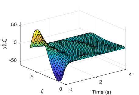
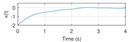
Figure 1: Time evolution of the reaction-diffusion part of the closed-loop system

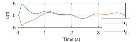
Figure 2: Time evolution of the ODE part of the closed-loop system

Figure 3: Command effort of the closed-loop system

VII Conclusion

This paper discussed the feedback stabilization of a class of diagonal Infinite-Dimensional Systems (IDS) with delay boundary control. The proposed approach generalizes a design method formerly reported for a reaction-diffusion equation while proposing a simplification of the boundary control law. The method consists, via a spectral decomposition, in the synthesis of a state-feedback for a finite-dimensional subsystem capturing the unstable dynamics of the plant. Due to the input delay, the design of the control law on the truncated subsystem has been carried out by means of the Artstein transformation. Then, an adequate Lyapunov function has been introduced to assess that the control law designed on the truncated subsystem also ensures the stabilization of the original IDS. Furthermore, it has been shown that this Lyapunov function also allows the assessment of the Input-to-State Stability (ISS) of the closed-loop system with respect to distributed disturbances. Finally, this ISS property has been used to study the stability of the closed-loop IDS when interconnected with an Ordinary Differential Equation (ODE) that also satisfies an ISS property. Specifically, it has been shown that the satisfaction of a certain small gain condition ensures the stability of the IDS-ODE loop for the proposed delayed boundary control law.

[Regularity and time derivative of an infinite sum] Let $\left\{e_{n},\;n\in\mathbb{N}^{*}\right\}$ by a Hilbert basis of $\mathcal{H}$. Then, as $\left\{\phi_{n},\;n\in\mathbb{N}^{*}\right\}$ is a Riesz basis with associated biorthogonal set $\left\{\psi_{n},\;n\in\mathbb{N}^{*}\right\}$, there exists $T\in\mathcal{L}(\mathcal{H})$ such that $T^{-1}\in\mathcal{L}(\mathcal{H})$ and, for all $n\geq 1$, $\phi_{n}=Te_{n}$ and $\psi_{n}=(T^{-1})^{*}e_{n}$. Let $A\in\mathcal{C}^{1}(\mathbb{R}_{+};\mathcal{H})$ be given. We obtain that, for all $t\geq 0$,

$$\sum\limits_{k\geq 1}|\left<A(t),\psi_{k}\right>|^{2} =\sum\limits_{k\geq 1}|\left<A(t),(T^{-1})^{*}e_{k}\right>|^{2}$$

$$=\sum\limits_{k\geq 1}|\left<T^{-1}A(t),e_{k}\right>|^{2}$$

$$=\|T^{-1}A(t)\|_{\mathcal{H}}^{2}$$

$$=\left<T^{-1}A(t),T^{-1}A(t)\right>_{\mathcal{H}}.$$

Thus $\sum\limits_{k\geq 1}|\left<A,\psi_{k}\right>|^{2}\in\mathcal{C}^{1}(\mathbb{R}_{+};\mathbb{R})$ and we have for all $t\geq 0$,

$$\dfrac{\mathrm{d}}{\mathrm{d}t}\left[\dfrac{1}{2}\sum\limits_{k\geq 1}\left|\left<A(t),\psi_{k}\right>_{\mathcal{H}}\right|^{2}\right]$$

$$=\operatorname{Re}\left<T^{-1}\dfrac{\mathrm{d}A}{\mathrm{d}t}(t),T^{-1}A(t)\right>_{\mathcal{H}}$$

$$=\operatorname{Re}\left<T^{-1}\sum\limits_{k\geq 1}\left<\dfrac{\mathrm{d}A}{\mathrm{d}t}(t),\psi_{k}\right>_{\mathcal{H}}\phi_{k},T^{-1}\sum\limits_{l\geq 1}\left<A(t),\psi_{l}\right>_{\mathcal{H}}\phi_{l}\right>_{\mathcal{H}}$$

$$=\sum\limits_{k,l\geq 1}\operatorname{Re}\left\{\left<\dfrac{\mathrm{d}A}{\mathrm{d}t}(t),\psi_{k}\right>_{\mathcal{H}}\overline{\left<A(t),\psi_{l}\right>_{\mathcal{H}}}\left<T^{-1}\phi_{k},T^{-1}\phi_{l}\right>_{\mathcal{H}}\right\}$$

$$=\sum\limits_{k,l\geq 1}\operatorname{Re}\left\{\left<\dfrac{\mathrm{d}A}{\mathrm{d}t}(t),\psi_{k}\right>_{\mathcal{H}}\overline{\left<A(t),\psi_{l}\right>_{\mathcal{H}}}\left<e_{k},e_{l}\right>_{\mathcal{H}}\right\}$$

$$=\sum\limits_{k\geq 1}\operatorname{Re}\left\{\left<\dfrac{\mathrm{d}A}{\mathrm{d}t}(t),\psi_{k}\right>_{\mathcal{H}}\overline{\left<A(t),\psi_{k}\right>_{\mathcal{H}}}\right\}.$$

Noting that, for all $k\geq 1$,

$$\dfrac{\mathrm{d}}{\mathrm{d}t}\left[\dfrac{1}{2}\left|\left<A(t),\psi_{k}\right>_{\mathcal{H}}\right|^{2}\right]=\operatorname{Re}\left\{\left<\dfrac{\mathrm{d}A}{\mathrm{d}t}(t),\psi_{k}\right>_{\mathcal{H}}\overline{\left<A(t),\psi_{k}\right>_{\mathcal{H}}}\right\},$$

we deduce that $\sum\limits_{k\geq N_{0}+1}|\left<A,\psi_{k}\right>|^{2}\in\mathcal{C}^{1}(\mathbb{R}_{+};\mathbb{R})$.

References

- [1] Z. Artstein, “Linear systems with delayed controls: a reduction,” IEEE Transactions on Automatic Control, vol. 27, no. 4, pp. 869–879, 1982.
- [2] D. Bresch-Pietri, C. Prieur, and E. Trélat, “New formulation of predictors for finite-dimensional linear control systems with input delay,” Systems & Control Letters, vol. 113, pp. 9–16, 2018.
- [3] O. Christensen et al., An Introduction to Frames and Riesz Bases. Springer, 2016.
- [4] J.-M. Coron and E. Trélat, “Global steady-state controllability of one-dimensional semilinear heat equations,” SIAM Journal on Control and Optimization, vol. 43, no. 2, pp. 549–569, 2004.
- [5] ——, “Global steady-state stabilization and controllability of 1D semilinear wave equations,” Communications in Contemporary Mathematics, vol. 8, no. 04, pp. 535–567, 2006.
- [6] R. F. Curtain and H. Zwart, An Introduction to Infinite-Dimensional Linear Systems Theory. Springer Science & Business Media, 2012, vol. 21.
- [7] E. Fridman, S. Nicaise, and J. Valein, “Stabilization of second order evolution equations with unbounded feedback with time-dependent delay,” SIAM Journal on Control and Optimization, vol. 48, no. 8, pp. 5028–5052, 2010.
- [8] E. Fridman and Y. Orlov, “Exponential stability of linear distributed parameter systems with time-varying delays,” Automatica, vol. 45, no. 1, pp. 194–201, 2009.
- [9] W. Kang and E. Fridman, “Boundary control of delayed ODE-heat cascade under actuator saturation,” Automatica, vol. 83, pp. 252–261, 2017.
- [10] I. Karafyllis and M. Krstic, Input-to-State Stability for PDEs. Springer, 2019.
- [11] M. Krstic, “Control of an unstable reaction-diffusion PDE with long input delay,” Systems & Control Letters, vol. 58, no. 10-11, pp. 773–782, 2009.
- [12] H. Lhachemi and R. Shorten, “ISS property with respect to boundary disturbances for a class of Riesz-spectral boundary control systems,” arXiv preprint arXiv:1810.03553, 2018.
- [13] S. Nicaise, C. Pignotti et al., “Stabilization of the wave equation with boundary or internal distributed delay,” Differential and Integral Equations, vol. 21, no. 9-10, pp. 935–958, 2008.
- [14] S. Nicaise and J. Valein, “Stabilization of the wave equation on 1-D networks with a delay term in the nodal feedbacks,” NHM, vol. 2, no. 3, pp. 425–479, 2007.
- [15] S. Nicaise, J. Valein, and E. Fridman, “Stability of the heat and of the wave equations with boundary time-varying delays,” Discrete and Continuous Dynamical Systems, vol. 2, no. 3, p. 559, 2009.
- [16] A. Pazy, Semigroups of Linear Operators and Applications to Partial Differential Equations. Springer Science & Business Media, 2012, vol. 44.
- [17] C. Prieur and E. Trélat, “Feedback stabilization of a 1D linear reaction-diffusion equation with delay boundary control,” IEEE Transactions on Automatic Control, no. to appear, 2019.
- [18] J.-P. Richard, “Time-delay systems: an overview of some recent advances and open problems,” Automatica, vol. 39, no. 10, pp. 1667–1694, 2003.
- [19] D. L. Russell, “Controllability and stabilizability theory for linear partial differential equations: recent progress and open questions,” Siam Review, vol. 20, no. 4, pp. 639–739, 1978.
- [20] O. Solomon and E. Fridman, “Stability and passivity analysis of semilinear diffusion pdes with time-delays,” International Journal of Control, vol. 88, no. 1, pp. 180–192, 2015.
- [21] E. D. Sontag, “Smooth stabilization implies coprime factorization,” IEEE Transactions on Automatic Control, vol. 34, no. 4, pp. 435–443, 1989.
- [22] A. Tanwani, S. Marx, and C. Prieur, “Local input-to-state stabilization of 1-D linear reaction-diffusion equation with bounded feedback,” in 23rd International Symposium on Mathematical Theory of Networks and Systems (MTNS2018), 2018, p. 6p.
- [23] J.-W. Wang and C.-Y. Sun, “Delay-dependent exponential stabilization for linear distributed parameter systems with time-varying delay,” Journal of Dynamic Systems, Measurement, and Control, vol. 140, no. 5, p. 051003, 2018.
- [24] K. Zhou and J. C. Doyle, Essentials of Robust Control. Prentice hall Upper Saddle River, NJ, 1998, vol. 104.