Solar wind charge exchange in cometary atmospheres

Abstract

Context. Solar wind charge-changing reactions are of paramount importance to the physico-chemistry of the atmosphere of a comet, mass-loading the solar wind through an effective conversion of fast light solar wind ions into slow heavy cometary ions.

Aims. To understand these processes and place them in the context of a solar wind plasma interacting with a neutral atmosphere, numerical or analytical models are necessary. Inputs of these models, such as collision cross sections and chemistry, are crucial.

Methods. Book-keeping and fitting of experimentally measured charge-changing and ionization cross sections of hydrogen and helium particles in a water gas are discussed, with emphasis on the low-energy/low-velocity range that is characteristic of solar wind bulk speeds ($<20$ keV u^-1/$2000$ km s^-1).

Results. We provide polynomial fits for cross sections of charge-changing and ionization reactions, and list the experimental needs for future studies. To take into account the energy distribution of the solar wind, we calculated Maxwellian-averaged cross sections and fitted them with bivariate polynomials for solar wind temperatures ranging from $10^{5}$ to $10^{6}$ K ($12-130$ eV).

Conclusions. Single- and double-electron captures by He²⁺ dominate at typical solar wind speeds. Correspondingly, single-electron capture by H⁺ and single-electron loss by H^- dominate at these speeds, resulting in the production of energetic neutral atoms (ENAs). Ionization cross sections all peak at energies above $20$ keV and are expected to play a moderate role in the total ion production. However, the effect of solar wind Maxwellian temperatures is found to be maximum for cross sections peaking at higher energies, suggesting that local heating at shock structures in cometary and planetary environments may favor processes previously thought to be negligible. This study is the first part in a series of three on charge exchange and ionization processes at comets, with a specific application to comet 67P/Churyumov-Gerasimenko and the Rosetta mission.

1 Introduction

Over the past decades, evidence of charge-exchange reactions (CX) has been discovered in astrophysics environments, from cometary and planetary atmospheres to the heliosphere and to supernovae environments (Dennerl, 2010). They consist of the transfer of one or several electrons from the outer shells of neutral atoms or molecules, denoted M, to an impinging ion, noted Xⁱ⁺, where $i$ is the initial charge number of species X. Electron capture of $q$ electrons takes the form

$$\textnormal{X}^{i+}+\textnormal{M} \longrightarrow\textnormal{X}^{(i-q)+}+[\textnormal{M}]^{q+}.$$ (1)

From the point of view of the impinging ion, a reverse charge-changing process is the electron loss (or stripping); starting from species $\textnormal{X}^{(i-q)+}$, it results in the emission of $q$ electrons:

$$\textnormal{X}^{(i-q)+}+\textnormal{M} \longrightarrow\textnormal{X}^{i+}+[\textnormal{M}]\ +\ qe^{-}.$$ (2)

For $q=1$, the processes are referred to as one-electron charge-changing reaction; for $q=2$, two-electron or double charge-changing reactions, and so on. The qualifier ”charge-changing” encompasses both capture and stripping reactions, whereas ”charge exchange” or ”charge transfer” denote electron capture reactions only. Moreover, ”[M]” refers here to the possibility for compound M to undergo dissociation, excitation, and ionization, or a combination of these processes.

Charge exchange was initially studied as a diagnostic for man-made plasmas (Isler, 1977; Hoekstra et al., 1998). The discovery by Lisse et al. (1996) of X-ray emissions at comet Hyakutake C/1996 B2 was first explained by Cravens (1997) as the result of charge-transfer reactions between highly charged solar wind oxygen ions and the cometary neutral atmosphere. Since this first discovery, cometary charge-exchange emission has successfully been used to remotely $(i)$ measure the speed of the solar wind (Bodewits et al., 2004), $(ii)$ measure its composition (Kharchenko et al., 2003), and thus the source region of the solar wind (Bodewits et al., 2007; Schwadron & Cravens, 2000), $(iii)$ map plasma interaction structures (Wegmann & Dennerl, 2005), and more recently, $(iv)$ to determine the bulk composition of cometary atmospheres (Mullen et al., 2017).

Observations of charge-exchanged helium, carbon and oxygen ions were made during the Giotto mission flyby of comet 1P/Halley and were reported by Fuselier et al. (1991), who used a simplified continuity equation (as in Ip, 1989) to describe CX processes. Bodewits et al. (2004) reinterpreted their results with a new set of cross sections. More recently, the European Space Agency (ESA) Rosetta mission to comet 67P/Churyumov-Gerasimenko (67P) between August 2014 and September 2016 provided a unique opportunity for studying CX processes in situ for an extended period of time (Nilsson et al., 2015; Simon Wedlund et al., 2016). The observations need to be interpreted with the help of analytical and numerical models.

Charge state distributions and their evolution with respect to outgassing rate and cometocentric distance represent a proxy for the efficiency of charge-changing reactions at a comet such as 67P. The accurate determination of relevant charge-changing and total ionization cross sections is a pivotal preliminary step when these reactions are to be quantified and in situ observations are to be interpreted. Reviews of charge-changing cross sections exist, for example, for He²⁺ particle electron capture cross sections in a variety of molecular and atomic target gases (Hoekstra et al., 2006), or for track-structure biological applications at relatively high energies (Dingfelder et al., 2000; Uehara & Nikjoo, 2002). However, no critical and recent survey of charge-changing and ionization cross sections of helium and hydrogen particles in a water gas at solar wind energies is currently available. The goal of this paper is hence a critical review of experimental He and H charge-changing collisions with H₂O: in that, it complements the seminal study of Itikawa & Mason (2005) for electron collisions with water by providing experiment-based datasets that space plasma modelers can easily implement, but also by assessing what future experimental work is needed.

In this study (Paper I), we first discuss the method we used to critically evaluate CX and ionization cross sections. A review of existing experimental charge-changing and ionization cross sections of hydrogen and helium species in a water gas is then presented in Sections 3 and 4, with a specific emphasis on low-energy values for typical solar wind energies. As H₂O was the most abundant cometary neutral species during most of the Rosetta mission (Läuter et al., 2019), we consider this species only. We identify laboratory data needs that are required to bridge the gaps in the existing experimental results. Polynomial fits for the systems $(\textnormal{H}^{+},\leavevmode\nobreak\ \textnormal{H},\leavevmode\nobreak\ \textnormal{H}^{-})-\textnormal{H}_{2}\textnormal{O}$ and $(\textnormal{He}^{2+},\leavevmode\nobreak\ \textnormal{He}^{+},\leavevmode\nobreak\ \textnormal{He})-\textnormal{H}_{2}\textnormal{O}$ are proposed. Recommended values are also tabulated for ease of book-keeping. In order to take into account the effect of the thermal energy distribution of the solar wind, Maxwellian-averaged charge-changing and ionization cross sections are discussed with respect to solar wind temperatures in Sect. 5.

In a companion paper (Simon Wedlund et al., 2019, hereafter Paper II), we then develop, based on these cross sections, an analytical model of solar wind charge-changing reactions in astrophysical environments, which we apply to solar wind-cometary atmosphere interactions. An interpretation of the Rosetta ion and neutral datasets using this model is given in a separate iteration, namely Simon Wedlund et al. (2018), hereafter Paper III.

2 Method

We detail in this section the method we used in selecting cross sections. In this work, we only consider experimental inelastic (ionization and charge exchange) cross sections. Elastic (scattering) cross sections may play an important role at low impacting energies (a few tens of eV), leading to energy losses of the projectile species and to local heating. However, as shown in Behar et al. (2017), solar wind ions, although highly deflected around the comet, do not display any significant slowing down at the position of Rosetta in the inner coma: to a first approximation, elastic collisions may thus be neglected.

Because H₂O was the main neutral species around comet 67P during the span of the Rosetta mission, we only consider H₂O molecules as targets. However, it is important to remember that cometary environments contain other abundant molecules (CO₂, CO, and O₂, see Läuter et al., 2019), and that parent molecules also photodissociate into H, O, C, H₂ , or OH fragments, which may in turn become dominant at very large cometocentric distances (typically more than $100\,000$ km for heliocentric distances below $2$ AU, or astronomical units, see Combi et al., 2004). Because charge-transfer reactions are a cumulative process and depend on the column of atmosphere traversed (see Simon Wedlund et al., 2016) and because some of these reactions may be resonant, their effect on the charge state distribution can potentially be large. Estimates of these effects using an analytical model of charge exchange at comets are discussed in Paper II.

2.1 Approach

In selecting and choosing our chosen set of cross sections, our method consists of five steps:

• Measurements Survey of the currently published experimental cross sections $\sigma_{if}$ in H₂O vapor, with $i$ and $f$ the initial and final charge states of the projectile species considered. For example, $\sigma_{21}$ is the cross section of electron capture reaction $\textnormal{He}^{2+}\rightarrow\textnormal{He}^{+}$.

• Uncertainties. Associated experimental uncertainties reported by the experimental teams. Sometimes, as in the case of Greenwood et al. (2004), these uncertainties are statistical confidence intervals ($2\sigma$ standard deviation).

• Selection. Selection of the chosen cross-section set, with emphasis on filling the low- and high-energy parts of the data. When experimental results are missing, we use the so-called additive rule (sometimes referred to as the ”Bragg rule”).

• Fit and validity. Polynomial fits of the form

  $$\log_{10}(\sigma_{if})=\sum_{j=0}^{n}{p_{j}\,(\log_{10}\varv_{i})^{j}}$$ (3)

  are applied in a least-squares sense on the selected datasets as a function of impact speed $\varv_{i}$. Coefficients $p_{j}$ are the polynomial coefficients and $n$ is the degree of the polynomial fit. The degree of the fit is chosen so that in the energy range of the measurements and for every energy channel, fit residuals never exceed $15\%$ of the measurements. A descriptive confidence level for the fit is also given, based on the agreement between the collected datasets and their respective datasets. It ranges from low ($>75\%$ uncertainty) to medium ($25-75\%$ uncertainty) and high ($<25\%$ uncertainty). Subscript $i$ in speeds and energies refers to ”impactor” or ”initial state”, that is, the projectile speed or energy.

• Further work. We give recommendations on the necessary experimental work to be performed, and the energy range most critical to investigate.

2.2 Extrapolations: the additive rule

In several cases, we used the ”additive rule” (that we refer to as AR in the following) to reconstruct missing H₂O datasets. First expressed by Bragg & Kleeman (1905) when investigating the stopping power of He²⁺ in various atoms and molecules, it states that the stopping power of a molecule is, in a first approximation, equal to the sum of its individual atomic stopping powers. The AR hence assumes no intra-molecular effects, which leads to low predictability at energies where inelastic processes take place (Thwaites, 1983). For H₂O targets, this translates as

$$\sigma_{if}(\textnormal{H}_{2}\textnormal{O})\sim 2\sigma_{if}(\textnormal{H})+\sigma_{if}(\textnormal{O})\sim\sigma_{if}(\textnormal{H}_{2})+\sigma_{if}(\textnormal{O}_{2})/2.$$ (4)

At high impact energy, the AR for charge-changing cross sections has been well verified for protons and helium particles in many gases (Toburen et al., 1968; Dagnac et al., 1970; Sataka et al., 1990; Endo et al., 2002), both for electron capture (Itoh et al., 1980a) and for electron loss (Itoh et al., 1980b). However, since this description is only empirical and not physical, one must be careful in applying it too systematically. For instance, it is well known that the AR breaks down for heavy ion collisions on complex molecules (Wittkower & Betz, 1971; Bissinger et al., 1982), for electron capture emission cross sections (Bryan et al., 1990), or at low energies (see Tolstikhina et al., 2018).

In the case of low-energy extrapolations, the AR is not expected to be fulfilled because the molecular electrons move much faster than the projectile ion, and thus may follow the motion of the ion and adjust to it. Such an effect can be seen, for instance, in the low-energy electron capture cross-section measurements of Bodewits et al. (2006) on CO and CO₂ molecules, for which $\sigma_{21}$(CO)$>\sigma_{21}$(CO₂). When there were no experimental data, we used in this study the AR as an estimate for the cross sections at high energy and an indication of their magnitude at low energy, and always associated the retrieved cross sections with a high uncertainty. When we applied the AR, we used the most recent experimental results for other species such as H₂, O₂ , or O and made a linear combination of their individual cross section to estimate that of H₂O. In several cases, when H₂O experimental results were available, the AR yielded results that are very different (e.g., for $\sigma_{12}$ for the helium system, or for $\sigma_{01}$ and $\sigma_{0-1}$ for the hydrogen system), which lie typically within a multiplication factor $1-3$ of the H₂O results. In others, the AR is in good agreement (e.g., for $\sigma_{10}$ and $\sigma_{12}$ for the helium system, or, apparently, $\sigma_{-11}$ for the hydrogen system). Consequently, when necessary and possible, we scaled the added cross sections to existing H₂O measurements to fill critical gaps in the datasets at either low or high energies.

Many charge-exchange and ionization cross sections for atoms and simple molecular targets are available as part of the charge-changing database maintained at the Lomonosov Moscow State University (Novikov & Teplova, 2009). It is important to note that when available, cross sections for H₂ targets were preferred to those for H, in order to avoid resonant effects between protons and hydrogen atoms.

2.3 Fitting of reconstructed cross sections

Polynomial fits are here preferred to semi-empirical or more theoretical fits (Dalgarno, 1958; Green & McNeal, 1971) for their simplicity, versatility in describing the different processes, and standard implementation in complex physical models of cometary and astrophysical environments. Two broad categories of charge-exchange processes may take place: resonant (or symmetric) and non-resonant charge exchange (Banks & Kockarts, 1973). Resonant charge exchange, such as $\textnormal{X}^{+}\leavevmode\nobreak\ +\leavevmode\nobreak\ \textnormal{X}\leavevmode\nobreak\ \rightarrow\leavevmode\nobreak\ \textnormal{X}\leavevmode\nobreak\ +\leavevmode\nobreak\ \textnormal{X}^{+}$, with ion $\textnormal{X}^{+}$ impacting its neutral counterpart X, usually has large cross sections; it has been shown theoretically that they continue to increase with decreasing impacting energies down to zero energy, where they peak (Dalgarno, 1958). For resonant capture at very high energies, where electron double-scattering dominates the interaction, Belkić et al. (1979) showed with theoretical considerations that the behavior of cross sections followed a $\varv^{k}$ power law, with $k=11$. Conversely, non-resonant charge exchange peaks at non-zero velocity and is described by a more complex relation (Lindsay & Stebbings, 2005), with typical values at low (high) energies increasing (decreasing) as power laws of the velocity. We were able to use a simple polynomial fit of order $2-6$ to describe all charge-changing and ionization cross sections, which makes it easy to compare between them. The validity range of the fit was confined to the velocity range of available measurements. Where needed, smooth extrapolations of the fits were performed in power laws of the velocity down to $100$ km s^-1 and for very high energies; these extrapolations have large uncertainties and are only given for reference in the tables in the appendix.

We also note that in a cometary environment, resonant charge-exchange reactions such as $\textnormal{H}^{+}-\textnormal{H}$ may take place (Bodewits et al., 2004). For example, H and O are both present in the solar wind and in the cometary coma; at large cometocentric distances, cometary H and O atoms dominate the neutral coma because H₂O, CO₂ or CO will be fully photodissociated. Moreover, resonant processes usually have large cross sections. However, for a relatively low-activity comet such as comet 67P (outgassing rate lower than $10^{28}$ s^-1), and although the hydrogen cometo-corona extends millions of kilometers upstream, the solar wind proton densities will have diminished due to resonant charge exchange by less than $1\%$ by the time it reaches a cometocentric distances of $10\,000$ km. This point is further discussed in Paper II.

3 Experimental charge-changing cross sections for (H, He) particles in H₂O

Cross sections are given at typical solar wind speeds and are discussed in light of available laboratory measurements. Twelve cross sections, six listed in Sect. 3.1 for helium and six in Sect. 3.2 for hydrogen, are considered.

Starting with an incoming ion species $\textnormal{X}^{i}$ in an initial charge state $i$ colliding with neutral target M, and three possible final charge states $(i,\leavevmode\nobreak\ i-1,\leavevmode\nobreak\ i-2)$, the reactions can be written as

$$\sigma_{i,i-1}: \ \textnormal{X}^{i+} + \longrightarrow \ \textnormal{X}^{(i-1)+} + \ \textnormal{M}^{+}$$ M single capture

$$\sigma_{i,i-2}: \ \textnormal{X}^{i+} + \longrightarrow \ \textnormal{X}^{(i-2)+} + \ \textnormal{M}^{2+}$$ M double capture

$$\sigma_{i-1,i}: \ \textnormal{X}^{(i-1)+} + \longrightarrow \ \textnormal{X}^{i+} + \ \textnormal{M}+e^{-}$$ M single stripping

$$\sigma_{i-1,i-2}: \ \textnormal{X}^{(i-1)+} + \longrightarrow \ \textnormal{X}^{(i-2)+} + \ \textnormal{M}^{+}$$ M single capture

$$\sigma_{i-2,i}: \ \textnormal{X}^{(i-2)+} + \longrightarrow \ \textnormal{X}^{i+} + \ \textnormal{M}+2e^{-}$$ M double stripping

$$\sigma_{i-2,i-1}: \ \textnormal{X}^{(i-2)+} + \longrightarrow \ \textnormal{X}^{(i-1)+} + \ \textnormal{M}+e^{-}$$ M single stripping.

Figure 1 illustrates the six processes per impacting species (hydrogen, initial charge states $i=1,0,-1$, and helium, initial charge states $i=2,1,0$), with the chosen nomenclature for the charge-changing cross sections.

A molecular target such as H₂O may dissociate into atomic or molecular fragments through electron capture or stripping (see Luna et al., 2007; Alvarado et al., 2005, in H⁺ and He²⁺-H₂O collisions); similarly, the impacting species may become excited in the process (see Seredyuk et al., 2005, in He${}^{2+}-$H₂O collisions). For the remainder of this paper, only total charge-changing cross sections are considered, that is, the sum of all dissociation and excitation channels. In other words, we only consider the loss of solar wind ions, not the production of excited or dissociated ionospheric species.

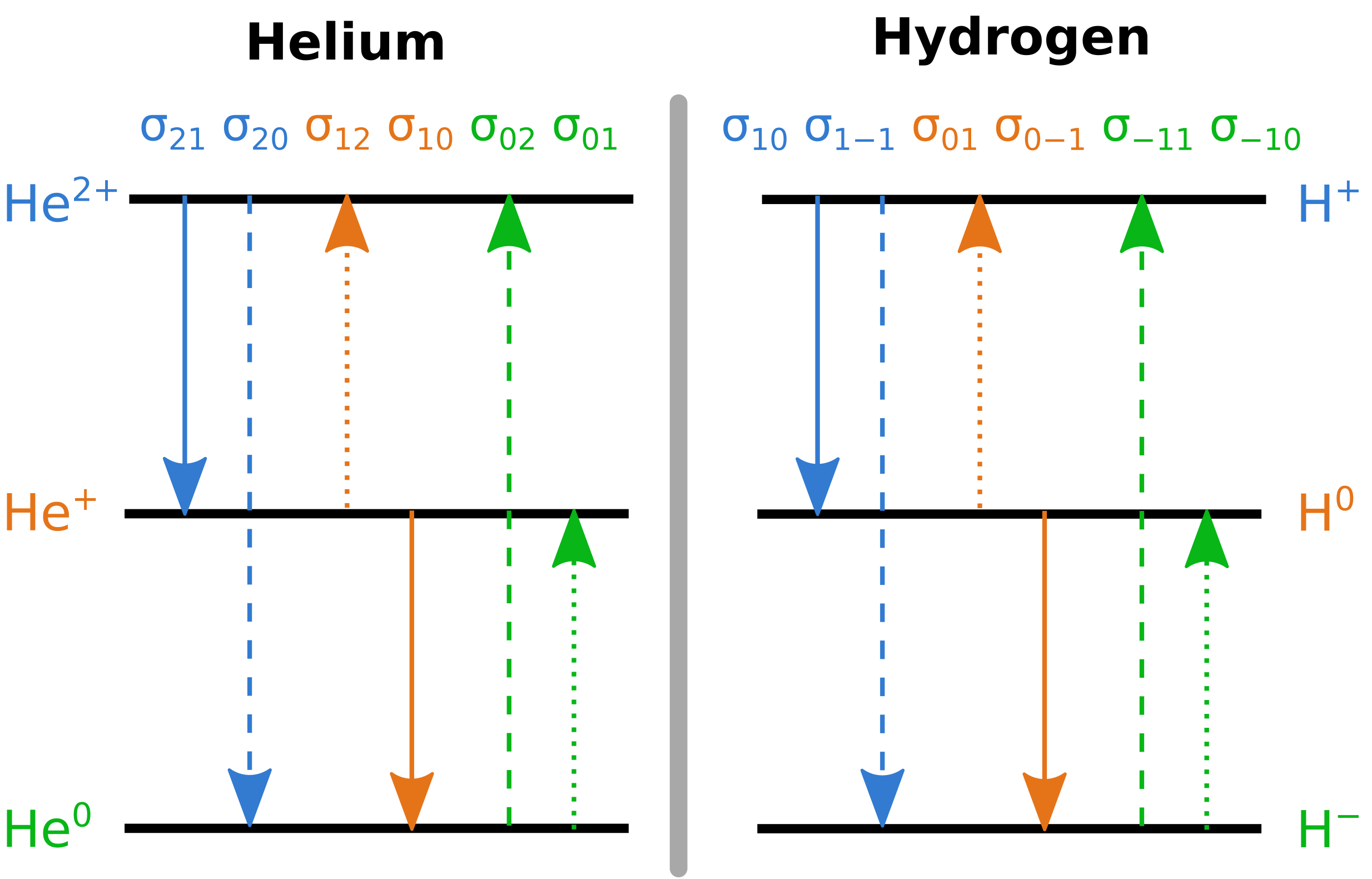
Figure 1: Charge-changing reactions for helium and hydrogen in a gas. One-electron capture processes are depicted with a solid line, one-electron loss processes with a dotted line, and double charge-changing reactions with a dashed line. Cross sections $\sigma_{ij}$ from initial charged state $i$ to final charged state $j$ are indicated.

3.1 Helium projectiles

The helium projectiles we considered are He²⁺, He⁺ and He⁰. Charge-changing cross sections for H₂O are presented, and our choice for each cross section is given. We note that all impact energies for helium are quoted in keV per amu (abbreviated keV/u), allowing us to compare the results of different experiments where sometimes ³He isotopes are used instead of the more common ⁴He.

Cross sections and their corresponding recommended fits are plotted in Fig. 2. Polynomial fitting coefficients are listed in Table 1.

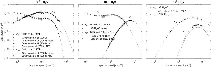
Figure 2: Experimental charge-changing cross sections for fast helium atoms and ions in a water gas as a function of impact speed. ”AR” refers to the ”additive rule”: when no experimental results for H₂O are available, results for H₂ and O₂ are combined to give an estimate (see text for details); experimental uncertainties for these estimates are at least $25$%. Recommended polynomial fits in thick continuous or dashed lines are also shown, whose coefficients are listed in Table 1. Smooth extrapolations at low and high energies are indicated as thin dotted lines.

Table 1: Recommended charge-changing cross section polynomial fits for (He²⁺, He⁺, and He⁰) projectiles colliding with H₂O vapor.

Cross section	Degree	Coefficients						Validity range		Confidence
[m2]	$n$	$p_{0}$	$p_{1}$	$p_{2}$	$p_{3}$	$p_{4}$	$p_{5}$	$\varv_{i}$ [km s-1]	$E_{i}$ [keV/u]
$\sigma_{21}$	$4$	$-129.6349$	$85.3069$	$-25.7100$	$3.50927$	$-0.18016$	-	$75-5350$	$0.03-150$	high
$\sigma_{20}$	$5$	$3327.3456$	$-3277.1313$	$1272.0445$	$-244.7593$	$23.35760$	$-0.88492$	$100-5350$	$0.05-150$	high
$\sigma_{12}$	$4$	$-314.9414$	$205.4565$	$-57.4465$	$7.3111$	$-0.34819$	-	$820-10\,000$	$3.50-520$	high
$\sigma_{10}$	$5$	$-5450.8180$	$4667.4695$	$-1592.4968$	$269.5820$	$-22.63262$	$0.75346$	$120-5000$	$0.08-130$	high
$\sigma_{02}$	$2$	$-245.4003$	$66.2165$	$-4.8686$	-	-	-	$3800-9300$	$75.0-450$	low
$\sigma_{01}$	$2$	$-98.7467$	$24.0604$	$-1.8252$	-	-	-	$310-10\,000$	$0.50-520$	low

3.1.1 He²⁺ – H₂O reactions

Reactions involving He²⁺ are the one-electron $\sigma_{21}$ and two-electron $\sigma_{20}$ captures. They are shown in Fig. 2 (left).

• Reaction $\sigma_{21}$ ($\textnormal{He}^{2+}\rightarrow\textnormal{He}^{+}$)

  • Measurements. Measurements of the one-electron capture by He²⁺ in a water gas were reported by Greenwood et al. (2004) in the $0.35-4.67$ keV/u energy range and by Rudd et al. (1985b) for $E_{i}=5-150$ keV/u (for ³He isotopes). Greenwood et al. (2000) also made measurements up to $6.67$ keV/u): their values are in excellent agreement with the subsequent results from the same team, except at $0.67$ keV/u ($\varv_{i}=360$ km s^-1), where it is about $25$% smaller. We note that Greenwood et al. (2004) provide recommended values that extend the valid range to $0.052-5.19$ keV/u ($100-1000$ km s^-1). At $5$ and $7.5$ keV/u, Rudd et al. (1985b) appear to underestimate the cross section by about $35$% with respect to that measured by Greenwood et al. (2000). Seredyuk et al. (2005) and Bodewits et al. (2006) measured state-selective charge-exchange cross sections between $0.025$ keV/u and $12$ keV using two complementary techniques (fragment ion spectroscopy, and translational energy spectrometry, or TES): below $0.25$ keV/u, capture into the He${}^{+}(n=1)$ state dominates, whereas capture into the He${}^{+}(n=2)$ state is dominant above this energy. Their total TES cross-section results were normalized to those of Greenwood et al. (2004), and display a matching energy-dependence with respect to the reference measurements.

  • Uncertainties. On average, uncertainties are about $10$% at low energies (Greenwood et al., 2004; Seredyuk et al., 2005) ($15-25$% below $0.3$ keV/u, $95\%$ confidence interval) and $12$% at high energies (Rudd et al., 1985b).

  • Selection. All datasets connect rather well at their common limit, if we discard the Rudd et al. (1985b) measurements below $8$ keV/u. We chose to use the values of Seredyuk et al. (2005) between $0.025-2$ keV/u, those of Greenwood et al. (2004) between $2-5.19$ keV/u supplemented up to $6.67$ keV/u by those of Greenwood et al. (2000), and we extend the set to energies above $10$ keV/u with those of Rudd et al. (1985b).

  • Fit and validity. A least-squares polynomial fit of degree $3$ in $\log_{10}$ of the He²⁺ speed $\varv_{i}$ was performed. Expected validity range $\varv_{i}=75-5350$ km s^-1 ($E_{i}=0.03-150$ keV/u). Confidence: high.

  • Further work. Need for very low-energy measurements, that is, for $E_{i}<0.02$ keV/u.

• Reaction $\sigma_{20}$ ($\textnormal{He}^{2+}\rightarrow\textnormal{He}^{0}$)

  • Measurements. Cross sections for the two-electron capture by He²⁺ from water vapor were experimentally measured by Greenwood et al. (2004) for $E_{i}=0.35-4.67$ keV/u and by Rudd et al. (1985b) between $5$ and $150$ keV/u. As for $\sigma_{21}$, Greenwood et al. (2004) gave fitted recommendations, extending their dataset to $0.052-5.19$ keV/u.

  • Uncertainties. Uncertainties range on average between $20$% below $5$ keV/u ($30-40$% below $0.3$ keV/u) (Greenwood et al., 2004) to $16$% above it (Rudd et al., 1985b).

  • Selection. Although as previously, Rudd et al. (1985b) do seem to underestimate the cross section at $5$ keV/u by about $30$%, both datasets join together well if we discard this first data point. We chose to use the Greenwood et al. (2004) recommendation for $E_{i}=0.052-5.19$ keV/u and Rudd et al. (1985b) for $E_{i}>5$ keV/u.

  • Fit and validity. A polynomial fit of order $5$ best represents the datasets. Expected validity range: $\varv_{i}=100-5350$ km s^-1 ($E_{i}=0.05-150$ keV/u). Confidence: high.

  • Further work. Need for very low-energy measurements, that is, for $E_{i}<0.1$ keV/u.

3.1.2 He⁺ – H₂O reactions

Reactions involving He⁺ ions are the one-electron loss $\sigma_{12}$ and the one-electron capture $\sigma_{10}$. They are shown in Fig. 2 (middle).

• Reaction $\sigma_{12}$ ($\textnormal{He}^{+}\rightarrow\textnormal{He}^{2+}$)

  • Measurements. Rudd et al. (1985d) measured the one-electron loss cross section for He⁺ in water in the $3.50-112.5$ keV/u ($820-4640$ km s^-1) range. No measurements are available below or above these energies.

  • Uncertainties. Uncertainties are $21-33$% on average (Rudd et al., 1985d).

  • Selection. We chose to use the measurements by Rudd et al. (1985d), and following the recommendation of Uehara & Nikjoo (2002), we used the additive rule with the cross sections of Sataka et al. (1990) in H₂ and O₂ at energies between $75$ and $450$ keV/u to define the peak of the cross section at high energies. At overlapping energies, the reconstructed cross section $\sigma(\textnormal{H}_{2})+\sigma(\textnormal{O}_{2})/2$ is lower than that measured by Rudd et al. (1985d) in H₂O: the latter measurements at $75$ keV/u were used to calibrate the former, resulting in a constant multiplication factor of $1.64$ for the H₂O dataset at high energies reconstructed from Sataka et al. (1990).

  • Fit and validity. A polynomial fit in $\log_{10}$ of order $4$ was used. Validity range: $\varv_{i}=820-10\,000$ km s^-1 ($E_{i}=3.5-520$ keV/u). Confidence: high. Further work. Need for low- ($0.01<E_{i}<5$ keV/u) and high-energy ($E_{i}>100$ keV/u) measurements.

• Reaction $\sigma_{10}$ ($\textnormal{He}^{+}\rightarrow\textnormal{He}^{0}$)

  • Measurements. Measurements of the one-electron capture cross section of fast He⁺ ions in water were made by Koopman (1968) between $0.2$ and $1.4$ keV/u energy, (Rudd et al., 1985d) in the $1.25-112.5$ keV/u ($490-4640$ km s^-1) range and by Greenwood et al. (2000) for $0.3-1.7$ keV/u ($253-565$ km s^-1). The results reported by Koopman (1968) are a factor $7.15$ lower than those of Greenwood et al. (2000) at their closest common energy ($0.33$ keV/u), but are nonetheless qualitatively similar in shape and energy behavior.

  • Uncertainties. Uncertainties are below $7$% for $E_{i}<1.7$ keV/u (Greenwood et al., 2000) and span $14-20$% for $E_{i}>2$ keV/u (Rudd et al., 1985d). Koopman (1968) claimed an uncertainty of $20$%.

  • Selection. The three datasets significantly differ in their common energy range ($>30$%, to almost an order of magnitude for Koopman, 1968). Because the Greenwood et al. (2000) measurements have a higher accuracy, we chose this dataset below $1.7$ keV/u and used Rudd et al. (1985d)’s for $E_{i}\geq 2.5$ keV/u. As remarked by Koopman (1968), the cross section is expected to continue to rise with diminishing energies, which may be due to a near-resonant process involving highly excited states of H₂O⁺. This tendency is also seen with electron capture by He⁺ impinging on a O₂ gas (Mahadevan & Magnuson, 1968). We therefore supplemented our data at low energy with an adjustment of the Koopman (1968) measurement at $73$ eV/u ($118$ km s^-1) by multiplying by a calibrating factor of $7.15$ ($\sigma_{10}^{\textnormal{adj}}\approx 9\times 10^{-20}$ m²), and placing less weight on this particular dataset because of the large uncertainties. We note that the additive rule using the results of Rudd et al. (1985c) for H₂ and O₂ agress well with the measurements made in H₂O (within the experimental uncertainties).

  • Fit and validity. Polynomial fit of order $5$ was performed. Validity range: $\varv_{i}=120-5000$ km s^-1 ($E_{i}=0.08-130$ keV/u). Confidence: high.

  • Further work. Need for measurements in the very low-energy range, that is, $E_{i}<0.5$ keV/u.

3.1.3 He⁰ – H₂O reactions

The reactions involving the neutral atom He⁰ are the two-electron $\sigma_{02}$ and one-electron $\sigma_{01}$ losses. They are shown in Fig. 2 (right).

• Reaction $\sigma_{02}$ ($\textnormal{He}^{0}\rightarrow\textnormal{He}^{2+}$)

  • Measurements. No measurement of the two-electron loss cross section for helium atoms in a water gas has been reported.

  • Uncertainties. N/A.

  • Selection. Because of the lack of measurements, we chose to use the additive rule so that $\sigma_{02}$(H₂O)$\sim\sigma_{02}$(H₂)+$\sigma_{02}$(O${}_{2})/2$. For H₂ and O₂, and following Uehara & Nikjoo (2002), we used the measurements of Sataka et al. (1990) ($75-450$ keV/u), which were performed around the cross-section peak with an uncertainty below $7$%. The composite fit of Uehara & Nikjoo (2002) is within a factor $2$ and extends down in energies to about $8.5$ keV.

  • Fit and validity. A polynomial fit of order $2$ was performed. Validity range: $\varv_{i}=3800-9300$ km s^-1 ($E_{i}=75-450$ keV/u). Confidence: low.

  • Further work. Need of measurements at any energy, with priority for $0.05<E_{i}<500$ keV/u.

• Reaction $\sigma_{01}$ ($\textnormal{He}^{0}\rightarrow\textnormal{He}^{+}$)

  • Measurements. No measurement of the one-electron loss cross section for helium atoms in a water gas has been reported.

  • Uncertainties. N/A.

  • Selection. Because of the lack of measurements, we chose to use the additive rule so that $\sigma_{01}$(H₂O)$\sim\sigma_{01}$(H₂)+$\sigma_{01}$(O${}_{2})/2$. For H₂, we used the recommendation of Barnett et al. (1990) (who analyzed all measurements prior to 1990) in the $0.5-10^{3}$ keV/u energy range and supplemented them by the more recent measurements of Sataka et al. (1990) ($75-450$ keV/u), which are both in excellent agreement. For O₂, we used the results of Allison (1958) between $1$ and $50$ keV/u and Sataka et al. (1990) between $75$ and $450$ keV/u; these datasets connect very well around $60$ keV/u. Associated uncertainties of separate cross sections are better than $10$%.

  • Fit and validity. A polynomial fit of order $2$ was performed. Validity range: $\varv_{i}=310-10\,000$ km s^-1 ($E_{i}=0.50-520$ keV/u). Confidence: low.

  • Further work. Need of measurements at any energy, with priority for $0.05<E_{i}<500$ keV/u.

3.1.4 Discussion

Figure 2 shows that all charge-changing cross sections peak at values around $10^{-19}-10^{-20}$ m². Except for the capture cross sections $\sigma_{20}$ (He${}^{2+}\rightarrow$He) and $\sigma_{10}$ (He${}^{+}\rightarrow$He), which display a peak at speeds below $100$ km s^-1, the main peak of all other cross sections is situated at speeds higher than $1000$ km s^-1. $\sigma_{21}$ (He${}^{2+}\rightarrow$He⁺) is the largest cross section between $400$ and $3500$ km s^-1 (peak at $1.5\times 10^{-19}$ m²), whereas at low speeds, both double- and single-electron captures $\sigma_{20}$ and $\sigma_{10}$ for He²⁺ and He⁺ impactors become dominant, reaching values of about $1\times 10^{-19}$ m² at $100$ km s^-1. Comparatively, the electron-loss cross sections from atomic He and from He⁺ start to become significant at speeds above $3000$ km s^-1, where they reach a maximum and where electron capture cross sections start to decrease. The largest of these cross sections, stripping cross section $\sigma_{01}$, reaches values of $3.5\times 10^{-20}$ m² at its peak.

3.2 Hydrogen projectiles

The hydrogen projectiles we considered are H⁺, H⁰ , and H^-. Charge-changing cross sections for H₂O are presented, and our choice for each cross section is given, following the template of Sect. 3.1.

The cross sections and their corresponding recommended fits are plotted in Fig. 3. Polynomial fit coefficients are listed in Table 2.

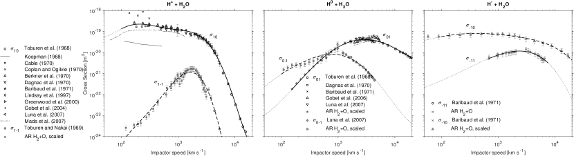
Figure 3: Experimental charge-changing cross sections for fast hydrogen atoms and ions in a water gas as a function of impact speed. ”AR” refers to the ”additive rule”: when no experimental results for H₂O are available, results for H₂ and O₂ are combined to give an estimate (see text for details); experimental uncertainties for these estimates are at least $25$%. Polynomial fits in thick continuous or dashed lines are also shown, whose coefficients are listed in Table 2. Smooth extrapolations at low and high energies are indicated as thin dotted lines.

Table 2: Recommended charge-changing cross-section polynomial fits for (H⁺, H⁰, H^-) projectiles colliding with H₂O vapor.

Cross section	Degree	Coefficients							Validity range		Confidence
[m2]	$n$	$p_{0}$	$p_{1}$	$p_{2}$	$p_{3}$	$p_{4}$	$p_{5}$	$p_{6}$	$\varv_{i}$ [km s-1]	$E_{i}$ [keV/u]
$\sigma_{10}$	$6$	$33151.6652$	$-34755.9561$	$15090.7461$	$-3475.4246$	$447.74484$	$-30.59282$	$0.865965$	$100-20\,000$	$0.05-2100$	high
$\sigma_{1-1}$	$6$	$23065.9322$	$-25763.6624$	$11868.1014$	$-2890.6324$	$392.69112$	$-28.20982$	$0.837012$	$100-7600$	$0.05-300$	low
$\sigma_{01}$	$4$	$332.2201$	$-247.4856$	$62.7381$	$-6.8495$	$0.27305$	-	-	$150-20\,000$	$0.10-2100$	medium
$\sigma_{0-1}$	$5$	$-1446.6760$	$1267.4240$	$-450.7229$	$79.8827$	$-7.03258$	$0.24532$	-	$100-4500$	$0.05-105$	low
$\sigma_{-11}$	$4$	$-121.2559$	$79.1328$	$-23.9740$	$3.2444$	$-0.16311$	-	-	$650-7600$	$2.20-300$	low
$\sigma_{-10}$	$5$	$403.3783$	$-383.3741$	$137.3481$	$-24.3561$	$2.14359$	$-0.07510$	-	$100-20\,000$	$0.05-2100$	low

3.2.1 H⁺–H₂O

Reactions involving H⁺ are the one-electron $\sigma_{10}$ and two-electron $\sigma_{1-1}$ captures. They are shown in Fig. 3 (left).

• Reaction $\sigma_{10}$ ($\textnormal{H}^{+}\rightarrow\textnormal{H}^{0}$)

  • Measurements. Since the end of the 1960s, many investigators have measured the one-electron capture cross section for protons in water (Koopman, 1968; Toburen et al., 1968; Berkner et al., 1970; Cable, 1970; Coplan & Ogilvie, 1970; Dagnac et al., 1970; Rudd et al., 1985a), concentrating on relatively high impact energies ($E_{i}>1$ keV, see Barnett et al., 1977). Recently, the cross section was remeasured by Lindsay et al. (1997) ($E_{i}=0.5-1.5$ keV) and by Greenwood et al. (2000) ($1.5-7$ keV). At high energies ($15<E_{i}<150$ keV), the recent measurements of Gobet et al. (2004) and Luna et al. (2007) agree well with those of Toburen et al. (1968). All measurements are in excellent agreement, except for those by Coplan & Ogilvie (1970), who seemed to overestimate their results by a factor $2-4$, and Koopman (1968), who underestimate them by about one order of magnitude. Finally, Baribaud et al. (1971) and Baribaud (1972) reported a value of $\sigma_{10}=(14\pm 8)\times 10^{-20}$ m² at $5$ keV, in good agreement with the other measurements. It is interesting to remark that the additive rule estimates using data in H₂ (Gealy & van Zyl, 1987a) and O (Van Zyl & Stephen, 2014) are $30$% lower on average than the direct measurements in H₂O.

  • Uncertainties. Measurement errors for the recent datasets are smaller than $10$% on average (Lindsay et al., 1997; Greenwood et al., 2000).

  • Selection. To extrapolate at energies below $500$ eV with a plausible energy dependence, we used the theoretical calculations of Mada et al. (2007) (Fig. 6, total charge-transfer cross section including all molecular axis collision orientations) increased by a factor $2.2$ to match Greenwood et al. (2000) and Lindsay et al. (1997) at $500$ eV. At high energies, the results of Luna et al. (2007), combined with those of Gobet et al. (2004), were chosen.

  • Fit and validity. A least-squares polynomial fit of degree $6$ in $\log_{10}$ of the proton speed $\varv_{i}$ was performed. Expected validity range $\varv_{i}=100-2\times 10^{4}$ km s^-1 ($E_{i}=0.05-2100$ keV). Confidence: high.

  • Further work. Measurements in the low-energy range $0.05\leavevmode\nobreak\ <E_{i}<5$ keV with good energy resolution are needed.

• Reaction $\sigma_{1-1}$ ($\textnormal{H}^{+}\rightarrow\textnormal{H}^{-}$)

  • Measurements. Only one measurement of the double-electron capture by protons in H₂O has been reported (Toburen & Nakai, 1969), and at high energies ($75<E_{i}<250$ keV). No low-energy measurements are available.

  • Uncertainties. Errors are reported to be $8$% in this high energy range.

  • Selection. Lacking data, we used the additive rule for the double capture by H₂ , which is well documented (Allison, 1958; McClure, 1963; Kozlov & Bondar’, 1966; Williams, 1966; Schryber, 1967; Toburen & Nakai, 1969; Salazar-Zepeda et al., 2010), and O₂ (Allison, 1958, given per atom of oxygen) at low proton impact energies. We supplement these estimates with the measurements in water by Toburen & Nakai (1969) at high energies. Since the measurements reported by Allison (1958) for O₂ are only made around $10$ keV, the behavior of H₂O at energies below is unknown. We chose to reconstruct the H₂O data around the peak with the additive rule and to multiply the H₂+O data at low energies by a factor $\sigma_{\textnormal{H}_{2}\textnormal{O}}/\sigma_{\textnormal{H}_{2}}=3.3$ to connect smoothly with the peak H₂O cross section. $1\sigma$ uncertainties for the AR dataset are indicated in the figure.

  • Fit and validity. A polynomial fit of order $6$ in $\log_{10}$ was performed on the overall reconstructed cross section. Because of the reconstructed AR dataset, the fit underestimates the cross-section peak by about $50\%$, although uncertainties are likely much larger. Validity range $\varv_{i}=100-7600$ km s^-1 ($E_{i}=0.05-300$ keV). Confidence: low.

  • Further work. Need of measurements for $0.05<E_{i}<100$ keV to confirm this estimate.

3.2.2 H⁰ – H₂O

Reactions involving H⁰ are the one-electron loss $\sigma_{01}$ and the one-electron capture $\sigma_{0-1}$. They are shown in Fig. 3 (middle).

• Reaction $\sigma_{01}$ ($\textnormal{H}^{0}\rightarrow\textnormal{H}^{+}$)

  • Measurements. Dagnac et al. (1969, 1970) measured one-electron-loss cross sections for the hydrogen impact on H₂O between $1.5$ and $60$ keV, which are in excellent agreement in their common range with the newer values given by Luna et al. (2007) in the $15-90$ keV range, which include both reaction channels $\textnormal{H}\rightarrow\textnormal{H}^{+}+\textnormal{H}_{2}\textnormal{O}^{+}+2e$ and $\rightarrow\textnormal{H}^{+}+\textnormal{H}_{2}\textnormal{O}+e$. Baribaud et al. (1971) and Baribaud (1972) reported a value of $\sigma_{01}=(1.6\pm 0.8)\times 10^{-20}$ m² at $5$ keV in good agreement. Gobet et al. (2006) reported cross sections between $20$ and $150$ keV, whereas Toburen et al. (1968) made measurements between $100$ keV and $2500$ keV, all in excellent agreement.

  • Uncertainties. Uncertainties range from 30% ($1.5-5$ keV) to $12-15$% ($>5$ keV) (Dagnac et al., 1970; Luna et al., 2007) and are on the order of $25$% at very high energies (Gobet et al., 2006).

  • Selection. We used data from Dagnac et al. (1970) and Luna et al. (2007) between $1.5$ and $90$ keV. To extrapolate the behavior of the cross section at lower energies, we used the additive rule $\sigma_{01}$(H₂)+$\sigma_{01}$(O), using Gealy & van Zyl (1987b) for H impact on H₂ paired with data reported by Van Zyl & Stephen (2014) for H impact on O (both with uncertainties of about $15-25$%) between $0.125$ and $2$ keV. At $2$ keV energy, the AR values overestimate the measurements of Dagnac et al. (1970) by a factor $3.8$ on average; we chose to use the scaled AR cross section to estimate the low-energy dependence below $1.5$ keV.

  • Fit and validity. A polynomial fit of order $4$ in $\log_{10}$ was performed on the chosen (H, H₂O) electron-loss cross sections. The expected validity range is $\varv_{i}=150-2\times 10^{4}$ km s^-1 ($0.1-2100$ keV). This simple fit compares well to that performed by Uehara et al. (2000). Confidence: medium.

  • Further work. Need for measurements for $0.05<E_{i}<5$ keV.

• Reaction $\sigma_{0-1}$ ($\textnormal{H}^{0}\rightarrow\textnormal{H}^{-}$)

  • Measurements. State-selective time-of-flight measurements of the one-electron capture cross section for H in water were recently made by Luna et al. (2007) in the $8-100$ keV range, which likely is above the cross-section peak.

  • Uncertainty. Uncertainties are on average $10$%.

  • Selection. Between $8$ and $100$ keV, we adopted the summed cross section over all target product channels of Luna et al. (2007). To extend these measurements, we chose to use the additive rule for H₂ and O, that is, at low energies, data from Gealy & van Zyl (1987b) for H on H₂ paired with data from Van Zyl & Stephen (2014) for H on O. At high energies, we used the measurements of Hill et al. (1979) in H₂ and those of Williams et al. (1984) in O. Finally, we scaled the overall reconstructed H₂+O data points to reach the magnitude of the Luna et al. (2007) data using a varying multiplication factor $1.3-4.8$ that depends on energy between $8$ and $30$ keV, and a constant $\times 4.8$ factor below $8$ keV.

  • Fit and validity. A polynomial fit of order $5$ on the reconstructed dataset. Validity range $\varv_{i}=100-4500$ km s^-1 ($0.05-105$ keV). Confidence: medium (low below $8$ keV, high above).

  • Further work. Need for measurements at energies below the peak, for $0.05<E_{i}<10$ keV.

3.2.3 H^- – H₂O

The reactions involving the negative fast ion H^- are the two-electron $\sigma_{-11}$ and the one-electron $\sigma_{-10}$ losses. They are shown in Fig. 3 (right).

• Reaction $\sigma_{-11}$ ($\textnormal{H}^{-}\rightarrow\textnormal{H}^{+}$)

  • Measurements. The only measurement found for the two-electron loss by H^- in H₂O is that of Baribaud et al. (1971), who reported a single cross section at $5$ keV for H₂O, $\sigma_{-11}=0.7\times 10^{-20}$ m².

  • Uncertainty. The reported error is about $30$% at $5$ keV.

  • Selection. Because of the lack of data, we adopted the additive rule $\sigma_{-11}$(H₂)+$\sigma_{-11}$(O₂)/2. For H₂, we used data from Geddes et al. (1980) in the energy range $1-300$ keV (dataset in excellent agreement for $\sigma_{-10}$ with that of Gealy & van Zyl, 1987b, thus giving good confidence on their $\sigma_{-11}$ values). For O₂, we used data reported by Williams et al. (1984) for $2.5<E_{i}<5$ keV, Fogel et al. (1957) and by Lichtenberg et al. (1980) for $E_{i}=50-227$ keV, which agree well in their common ranges.

  • Fit and validity. A polynomial fit of degree $4$ in $\log_{10}$ on the reconstructed (H^-, H₂O) two-electron-loss cross section. At $5$ keV, the additive rule fit is within $5\%$ of the reported value for H₂O (Baribaud et al., 1971). Validity range $\varv_{i}=650-7600$ km s^-1 ($2.2-300$ keV). Confidence: low.

  • Further work. Need for measurements at any energy, in priority in the energy range $0.1-100$ keV.

• Reaction $\sigma_{-10}$ ($\textnormal{H}^{-}\rightarrow\textnormal{H}^{0}$)

  • Measurements. The only measurement found for the one-electron loss by H^- in H₂O is that of Baribaud et al. (1971) (also in Baribaud, 1972), who reported a unique value at $5$ keV in H₂O, $\sigma_{-10}=7.5\times 10^{-20}$ m².

  • Uncertainty. The reported error is $13$% at $5$ keV.

  • Selection. Because of the lack of data, we chose to use the additive rule, $\sigma_{-10}$(H₂)+$\sigma_{-10}$(O₂)/2 and scaled it to the value of Baribaud et al. (1971) at $5$ keV. For H₂, the data from Geddes et al. (1980) ($1-300$ keV) and Hvelplund & Andersen (1982) ($300-3500$ keV) were joined. For O, data from Williams et al. (1984) ($2.5-250$ keV), which compare well with those from Lichtenberg et al. (1980) ($50-225$ keV), and Rose et al. (1958) ($400-1500$ keV) were adopted. At very low collision velocity, the energy of the center of mass is different from that of the ion energy measured in the laboratory frame. Huq et al. (1983) and Risley & Geballe (1974), reported by Phelps (1990), measured H^- total electron loss in H₂ from a threshold at $2.38$ eV to $200$ eV ($\varv_{i}=21-195$ km s^-1), and from $300$ eV to $10$ keV ($240-1400$ km s^-1), respectively. We note that in this energy range, single charge transfer dominates so that neutral hydrogen and negative molecular hydrogen ions are simultaneously produced: H^-+H${}_{2}\rightarrow$H+H${}_{2}^{-}$ (Huq et al., 1983). Correspondingly, Bailey & Mahadevan (1970) made measurements in O₂ in the range $0.007-0.34$ keV ($36-81$ km s^-1), with values of about $10^{-19}$ m²/atom. Compared to the one reported value for H₂O at $5$ keV, the reconstructed additive rule cross section overestimates the efficiency of the electron detachment by a factor $2.3$, which we chose as our scaling factor. The validity of such a scaling at one energy to extrapolate the values at other energies is likely subject to large uncertainties, which cannot be precisely assessed for lack of experimental or theoretical data.

  • Fit and validity. A polynomial fit of degree $5$ in $\log_{10}$ on the reconstructed (H^-, H₂O) one-electron-loss cross section, scaled to the value of Baribaud et al. (1971) at $5$ keV. Validity range $\varv_{i}=100-20\,000$ km s^-1 ($E_{i}=0.05-2100$ keV). Confidence: low.

  • Further work. Need for measurements at any energy, in priority above threshold, so that $0.1<E_{i}<100$ keV.

3.2.4 Discussion

Figure 3 shows the charge-changing cross sections for (H⁺, H, H^-). The dominant process below about $2000$ km s^-1 solar wind speed is electron capture $\sigma_{10}$ of H⁺, which reaches a maximum value of about $2\times 10^{-19}$ m². A second process of importance is electron stripping $\sigma_{-10}$ of H^- , reaching $0.8\times 10^{-19}$ m² at its peak at $400$ km s^-1. However, since only one measurement has been reported in water for this process, the additive rule is likely to give only a crude approximation at low speeds; that said, because H^- anions are populated by two very inefficient processes, this will likely result in a very small overall effect in the charge-state distributions (see Paper II). Consequently, at typical solar wind speeds, single-electron captures by H⁺ and H are expected to drive the solar wind charge- state distribution in a water gas.

4 Experimental ionization cross sections for (H, He) in H₂O

We present in this section the total ionization cross sections for the collisions of helium and hydrogen species with water molecules. Reviews at very high energies have been published over the past two decades with the development of Monte Carlo track-structure models describing how radiation interacts with biological tissues (Uehara & Nikjoo, 2002; Nikjoo et al., 2012).

Ionization cross sections are noted $\sigma_{ii}$ , where the initial charge state $i$ stays the same during the reaction (target ionization only). The reactions we consider in this section are thus

$$\sigma_{ii}: \ \textnormal{X}^{i+}+\textnormal{M}\longrightarrow\textnormal{X}^{i+}+\textnormal{[M]}^{q+}+qe^{-}\quad(\textnormal{X}^{i+}\rightarrow\textnormal{X}^{i+}),$$ (5)

with $q$ the number of electrons ejected from the neutral molecule M by a fast-incoming particle X. Because the initial solar wind ion distribution becomes fractionated on its path toward the inner cometary regions as a result of charge-transfer reactions, helium and hydrogen species are usually found in three charge states, namely Xⁱ⁺, X^(i-1)+ and X^(i-2)+, with $i$ the charge of the species. Because of the detection methods we used, experimentally reported cross sections are usually total electron production cross sections or positive-ion production cross sections (Rudd et al., 1985b; Gobet et al., 2006; Luna et al., 2007), which may contain contamination from transfer-ionization processes (as the overall charge is conserved). For protons in water, these charge-transfer processes are, for example,

$$\textnormal{H}^{+}+\textnormal{H}_{2}\textnormal{O}\longrightarrow\textnormal{H}+[\textnormal{H}_{2}\textnormal{O}]^{2+}+e^{-}.$$

The contribution of charge-transfer processes to the measured cross section may become non-negligible at low energies. However, at typical solar wind energies, the total electron production cross sections decrease rapidly as power laws, making the transfer-ionization contribution small in comparison to any of the single or double charge-changing reactions considered in Sect. 3. When the total charge-exchange and ionization rates are calculated from these two sets of cross sections, counting these minor charge-exchange reactions twice (a first time in the charge-exchange cross section and second time in the ionization) will therefore be minimized.

In ionization processes, the molecular target species M can also be dissociated into ionized fragments: for H₂O targets, ionization may lead to the formation of singly charged ions H⁺, H${}_{2}^{+}$, O⁺ and OH⁺ or even to that of doubly charged ions (e.g., O²⁺, as in Werner et al., 1995). In this section we only consider the total ionization cross section, which includes all dissociation paths of the target species, noted [M]^q+.

4.1 Helium + H₂O

Energies are given in keV per atomic mass unit (keV/u). Ionization cross sections for helium species are shown in Fig. 4. Corresponding polynomial fit parameters are given in Table 3.

• Reaction $\sigma_{22}$ ($\textnormal{He}^{2+}\rightarrow\textnormal{He}^{2+}$)

  • Measurements. Laboratory measurements were performed by Rudd et al. (1985b) between $10$ and $300$ keV/u ($1400-7500$ km s^-1) for the total electron production, and by Toburen et al. (1980) between $75$ keV/u and $500$ keV/u.The additive rule $\sigma$(H${}_{2})+\sigma$(O) with the datasets of Rudd et al. (1985b) in the same energy range yields results in excellent agreement with the water measurements (no measurements in H₂ and O₂ below $10$ keV were found).

  • Uncertainties. Uncertainties are $13\%$ below $300$ keV/u (Rudd et al., 1985b), and reach $20\%$ above (Toburen et al., 1980).

  • Selection. Since the datasets are complementary in energy and agree well with each other, we used both water measurements.

  • Fit and validity. A polynomial fit of order $4$ of the cross section as a function of the logarithm of the impact speed was performed. Expected validity range is $\varv_{i}=1400-10\,000$ km s^-1 ($E_{i}=10-520$ keV/u). Confidence: high.

  • Further work. Need for low-energy ($E_{i}<10$ keV/u) and very high-energy ($E_{i}>500$ keV/u) measurements.

• Reaction $\sigma_{11}$ ($\textnormal{He}^{+}\rightarrow\textnormal{He}^{+}$)

  • Measurements. Ionization cross sections have been measured by Rudd et al. (1985d) between $1.25$ and $112.5$ keV/u ($490-4650$ km s^-1), and by Toburen et al. (1980) between $75$ keV/u and $500$ keV/u. The additive rule using the measurements of Rudd et al. (1985c) in H₂ and O₂ agrees well at the cross-section peak and above ($>1$ keV/u) but increasingly diverges below (up to a factor $2$).

  • Uncertainties. Uncertainties are $20\%$ below $30$ keV/u and lower than $8\%$ in the $30-450$ keV/u range (Rudd et al., 1985d). At energies above $450$ keV/u, errors are on the order of $20\%$ (Toburen et al., 1980).

  • Selection. The two H₂O datasets overlap with each other and are in excellent agreement. We therefore used both datasets.

  • Fit and validity. A polynomial fit of order $4$ in $\log_{10}\varv_{i}$ was performed. Expected validity is $450-10\,000$ km s^-1 ($E_{i}=1-520$ keV/u). Confidence: high.

  • Further work. Need for very low-energy ($E_{i}<1$ keV/u) and very high-energy ($E_{i}>500$ keV/u) measurements.

• Reaction $\sigma_{00}$ ($\textnormal{He}^{0}\rightarrow\textnormal{He}^{0}$)

  • Measurements. No measurement of He⁰ impact ionization on water has been performed.

  • Uncertainties. -

  • Selection. To palliate the lack of measurements, Uehara & Nikjoo (2002) (reported in Nikjoo et al., 2012, with no alterations) proceeded in two steps with their Monte Carlo track-structure numerical model: at low energies (below $100$ keV/u), where He⁰ atoms dominate the composition of the charge distribution as a result of charge exchange, the authors adjusted the total ionization cross sections of He⁰+H₂O to match the total electronic stopping powers of the helium system tabulated in report $49$ of ICRU (Berger et al., 1993). At energies above $100$ keV/u, ionization cross sections of He⁰ were assumed to be equal to those of He⁺ measured by Toburen et al. (1980). Expected uncertainties according to Uehara & Nikjoo (2002) are of the order of $20\%$. These cross sections were chosen here. However, because no specific measurements have been made, we ascribe a low confidence level to this estimate, especially at typical solar wind energies.

  • Fit and validity. A polynomial fit in $\log_{10}\varv_{i}$ was performed. Expected validity range for such a composite estimate is $100-10\,000$ km s^-1 ($E_{i}=0.05-520$ keV/u). Confidence: low.

  • Further work. Measurements at any energy ($E_{i}>0.05$ keV/u) is needed.

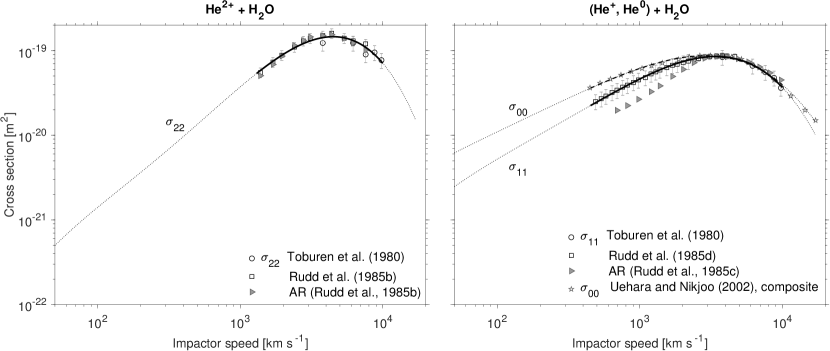
Figure 4: Experimental ionization cross sections for fast helium atoms and ions in a water gas as a function of impact speed. ”AR” refers to the additive rule: when no experimental results for H₂O are available, results for H₂ and O₂ are combined to give an estimate (see text for details); experimental uncertainties for these estimates are at least $25$%. As no experimental data are available for He⁰, the composite recommendation of Uehara & Nikjoo (2002) was chosen (see text). Polynomial fits in thick continuous and dashed lines are also shown, and the coefficients are listed in Table 3. Smooth extrapolations in power laws at low and high energies are indicated as thin dotted lines.

Table 3: Recommended ionization cross-section polynomial fits for (He²⁺, He⁺, He⁰) projectiles colliding with H₂O vapor.

Cross section	Degree	Coefficients					Validity range		Confidence
[m2]	$n$	$p_{0}$	$p_{1}$	$p_{2}$	$p_{3}$	$p_{4}$	$\varv_{i}$ [km s-1]	$E_{i}$ [keV/u]
$\sigma_{22}$	$4$	$-265.3697$	$176.7016$	$-48.3734$	$5.91427$	$-0.27030$	$1400-10\,000$	$10.0-520$	high
$\sigma_{11}$	$4$	$-169.8607$	$108.1412$	$-29.7492$	$3.66917$	$-0.16967$	$450-10\,000$	$1.06-520$	high
$\sigma_{00}$	$4$	$-87.3445$	$49.6893$	$-14.1573$	$1.82417$	$-0.08824$	$450-10\,000$	$1.06-520$	low

4.2 Hydrogen + H₂O

Ionization cross sections for hydrogen species are shown in Fig. 5. Corresponding polynomial fit parameters are given in Table 4.

• Reaction $\sigma_{11}$ ($\textnormal{H}^{+}\rightarrow\textnormal{H}^{+}$)

  • $\sigma_{11}$. Measurements. Over the past three decades, many experiments have been carried out on the ionization of water by fast protons. Toburen et al. (1980) compared their results at high energies for helium particles to those of protons (Toburen & Wilson, 1977) at $300$ and $500$ keV; proton cross sections were found to be about half those of He⁺. Rudd et al. (1985a) measured cross sections in the range $7-4000$ keV and Bolorizadeh & Rudd (1986a) in the $15-150$ keV range. These datasets are in good agreement with the more recent total ionization measurements by Werner et al. (1995) between $100$ and $400$ keV and those of Gobet et al. (2001) and Gobet et al. (2004), who focused on the production of dissociation fragments at $20$ to $400$ keV energies. Luna et al. (2007) reported total and partial ionization cross sections between $15-100$ and $500-3500$ keV; in their lower energy range, and similar to Werner et al. (1995), their total ionization cross sections also include contributions from the transfer ionization reaction $\textnormal{H}^{+}+\textnormal{H}_{2}\textnormal{O}\rightarrow\textnormal{H}+\textnormal{H}_{2}\textnormal{O}^{2+}+e$. When this is compared to the direct ionization measurements of Gobet et al. (2001) and Gobet et al. (2004), it appears that the total ionization cross section is probably not strongly affected by this additional contribution.

  • Uncertainties. Uncertainties are about $20\%$ between $7-15$ keV energy (Rudd et al., 1985a), and lower than $15\%$ at energies above $15$ keV (Luna et al., 2007).

  • Selection. We performed fits on all measurements listed above between $7$ and $4000$ keV. To extend the dataset to lower energies, the additive rule with the measurements of McNeal & Birely (1973) between $2-800$ keV and Rudd et al. (1985e) between $1-5000$ keV was used and scaled to match the results of Rudd et al. (1985a) at the cross-section peak; the composite $\sigma$(H₂)+$\sigma$(O${}_{2})/2$ cross section is on average $25\%$ smaller than the direct H₂O measurements.

  • Fit and validity. Polynomial fit of degree $5$ was performed on the reconstructed dataset. Expected validity range is $400-10\,000$ km s^-1 ($E_{i}=0.8-520$ keV/u). Confidence: high.

  • Further work. Need of laboratory measurements at low energies to very low energies ($0.05<E_{i}<10$ keV).

• Reaction $\sigma_{00}$ ($\textnormal{H}^{0}\rightarrow\textnormal{H}^{0}$)

  • Measurements. Laboratory measurements for the ionization of H₂O by fast hydrogen energetic neutral atoms (ENAs) were performed by Bolorizadeh & Rudd (1986b) between $20$ and $150$ keV. Electron loss to the continuum (ELC) cross sections were also concurrently calculated, which need to be subtracted from the total electron production cross sections (marked ”$\sigma_{-}$” in the terminology of Rudd’s team), as explained in detail in Gobet et al. (2006). Recently, the total target ionization cross section was measured by Gobet et al. (2006) using time-of-flight coincidence and imaging techniques and by Luna et al. (2007) using time-of-flight mass analysis, both above $15-20$ keV impact energy. As pointed out by Luna et al. (2007), the measurements of Gobet et al. (2006) at low collision energies are likely to have missed a portion of the proton beam scattered at high angles, suggesting an underestimation of their signal below about $30$ keV. Consequently, the measurements of Gobet et al. (2006) and Luna et al. (2007) diverge by a factor $2-3$ below $30$ keV, but they agree well above this limit. The ELC-corrected measurements of Bolorizadeh & Rudd (1986b) are larger by a factor $1.4-2$ above $50$ keV.

  • Uncertainties. Uncertainties are quoted to be about $20\%$ below $15$ keV by Bolorizadeh & Rudd (1986b), whereas Luna et al. (2007) claimed errors of about $10\%$ at all energies probed. Following Luna et al. (2007), we give the measurements by Gobet et al. (2006) a high uncertainty of $25\%$ because of the uncertainty in their calibration.

  • Selection. We chose the datasets of Luna et al. (2007) ($15-150$ keV) and that of Gobet et al. (2006), which is restricted to $50-100$ keV energies. To approximate the low-energy and high-energy dependence of the cross section, we used the additive rule $\sigma$(H₂)+$\sigma$(O${}_{2})/2$ with the datasets of McNeal & Birely (1973) between $0.1$ and $10$ keV, upscaled by $25\%$, as in the case of proton ionization cross sections (see $\sigma_{11}$ case above). This results in a smooth decrease at low energy, a trend that cannot be extrapolated further, however.

  • Fit and validity. A polynomial fit of degree $4$ was performed on the reconstructed dataset. Expected validity range: $140-9000$ km s^-1 ($E_{i}=0.1-420$ keV/u). Confidence: low (low at $\varv<1000$ km s^-1, medium above).

  • Further work. Need of laboratory measurements at any energy in the range $0.05-500$ keV.

• Reaction $\sigma_{-1-1}$ ($\textnormal{H}^{-}\rightarrow\textnormal{H}^{-}$)

  • Measurements. No measurement of impact ionization cross sections in collisions of H^- with H₂O has been performed or studied, to our knowledge. Similarly, no measurement has been found of ionization of H and O, as separate entities. Because charge fractions at comets do not favor the presence of H^- and because of the low expected fluxes, we avoid speculation. This species and its associated ionization cross section in water is left for further laboratory studies.

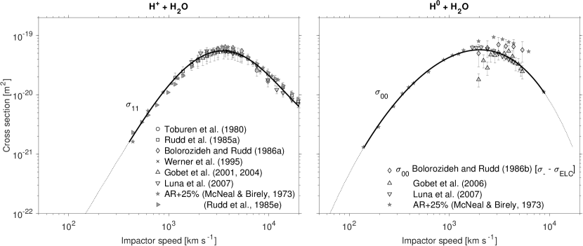
Figure 5: Experimental ionization cross sections for fast hydrogen atoms and protons in a water gas as a function of impact speed. ”AR” refers to the additive rule: when no experimental results for H₂O are available, results for H₂ and O₂ are combined to give an estimate (see text for details); experimental uncertainties for these estimates are at least $25$%. No measurement for the ionization of H₂O by H^- is available. Polynomial fits in thick lines are also shown, and the coefficients are listed in Table 4. Smooth extrapolations in power laws at low and high energies are indicated as thin dotted lines.

Table 4: Recommended ionization cross-section polynomial fits for (H⁺, H⁰) projectiles colliding with H₂O vapor.

Cross section	Degree	Coefficients						Validity range		Confidence
[m2]	$n$	$p_{0}$	$p_{1}$	$p_{2}$	$p_{3}$	$p_{4}$	$p_{5}$	$\varv_{i}$ [km s-1]	$E_{i}$ [keV/u]
$\sigma_{11}$	$5$	$-1437.4092$	$1233.0652$	$-429.3680$	$74.35337$	$-6.37862$	$0.216408$	$400-30\,000$	$0.84-4700$	high
$\sigma_{00}$	$4$	$-205.9851$	$114.3405$	$-27.6772$	$3.13079$	$-0.13835$	-	$140-10\,000$	$0.10-420$	low
$\sigma_{-1-1}$	-	-	-	-	-	-	-	-	-	no data

4.3 Discussion

Figures 4 and 5 show the total ionization cross sections for (He²⁺, He⁺, He⁰) and (H⁺, H⁰). The ionization cross sections for helium species are on average $1.5-2.5$ times larger than those for the hydrogen system. They peak for helium at $1.5\times 10^{-19}$ m² around $5000$ km s^-1 ($0.8\times 10^{-19}$ m², $2850$ km s^-1) for $\sigma_{22}$ ($\sigma_{11}$, respectively). For hydrogen, the cross sections peak at $0.5\times 10^{-19}$ m² around $3450$ km s^-1 ($0.6\times 10^{-19}$ m², $1950$ km s^-1) for $\sigma_{11}$ ($\sigma_{00}$). Consequently, the largest cross sections are encountered for the higher charge states of each system of species. However, for all ionization cross sections, their low-energy dependence is subject to large uncertainties as a result of a lack of experimental results.

5 Recommended Maxwellian-averaged cross sections for solar wind-cometary interactions

In the interplanetary medium, solar wind ion velocity distributions may be approximated by a Maxwellian at a constant temperature $T_{p}$ that typically is around $10^{5}$ K (Meyer-Vernet, 2012), or by a Kappa distribution in order to better take into account the tail of the velocity distribution (Livadiotis et al., 2018). For a Maxwellian distribution, which is a good first approximation, the temperature dependence with respect to heliocentric distance is such that $T_{p}=8\times 10^{4}\ R_{\textnormal{Sun}}^{-2/3}$ (Slavin & Holzer, 1981), with $R_{\textnormal{Sun}}$ the heliocentric distance in AU. This corresponds to thermal speeds $\varv_{\textnormal{th}}=\sqrt{3\,k_{B}T_{p}/m_{p}}$ of about $45$ km s^-1 at $1$ AU for protons of mass $m_{p}$, and half of that value for $\alpha$ particles: these values are much lower than the average ”undisturbed” solar wind speed of $400$ km s^-1. However, at the interface between the undisturbed solar wind and the cometary plasma environment, for instance at bow shock-like structures, considerable heating of the ions and electrons may occur simultaneously to the slowing down of the solar wind flow (Koenders et al., 2013; Simon Wedlund et al., 2017). Solar wind proton and electron temperatures during planetary shocks can reach values up to several $10^{6}$ K, for instance when interplanetary coronal mass ejections impact the induced magnetosphere of Venus ($T_{p}$ increasing up to $100$ eV, see Vech et al., 2015). Gunell et al. (2018) reported the first indication of a bow shock structure appearing for weak cometary outgassing rates at comet 67P: these structures were associated with a thermal spread of protons and $\alpha$ particles of a few $100$ km s^-1 ($T_{p}\gtrsim 10^{6}$ K). Deceleration and heating of the solar wind may in turn result in a spatially extended increase of the efficiency of the charge exchange and ionization (Bodewits et al., 2006). Bodewits and collaborators convolved a 3D drifting Maxwellian distribution with their He${}^{2+}-$H₂O electron capture cross sections and found that for solar wind velocities below $400$ km s^-1 and a temperature above $10^{6}$ K ($\varv_{\textnormal{th}}\sim 80$ km s^-1), the cross section could be increased by a factor $2-10$.

For low-activity comets such as comet 67P, Behar et al. (2017) calculated the velocity distributions of solar wind protons measured during the in-bound leg of the Rosetta mission. It is clear from their Fig. 2 that the velocity distribution functions cannot be approximated by a Maxwellian, which assumes dynamic and thermal equilibrium through collisions (ions thermalized at one temperature). Moreover, as CX reactions involve both the distribution of neutrals and ions, cross sections should be averaged over two velocity distributions, one for the neutrals, the other for the ions, with a reduced mass for the collision (Banks & Kockarts, 1973). Therefore, the following development only gives an indicator of global effects for increased solar wind temperatures at a comet assuming a Maxwellian velocity distribution, without taking into account the measured angular and energy distributions of the solar wind ions.

5.1 Method

In order to take the effects of a Maxwellian velocity distribution for the solar wind into account, energy-dependent cross sections $\sigma_{i}$ for solar wind impacting species $i$ can be Maxwellian-averaged over all thermal velocities $\varv$ following the descriptions of Banks & Kockarts (1973) and Bodewits et al. (2006):

$$\langle\sigma_{i}\rangle=\frac{\langle\sigma_{i}\,\varv\rangle}{\langle\varv\rangle}\ \hat{=}\ \sigma_{i,\textnormal{MACS}},$$ (6)

defining the Maxwellian-averaged cross section (MACS), $\sigma_{i,\textnormal{MACS}}$. The 3D drifting Maxwellian velocity distribution is defined as

$$f_{\textnormal{M}}(\@vec{v})=\left(\frac{m_{i}}{2\pi\,k_{B}T_{i}}\right)^{3/2}\ \exp\left[-\frac{m_{i}}{2k_{B}T_{i}}\left(\@vec{v}-\@vec{v}_{d}\right)^{2}\right],$$ (7)

with $\@vec{v}_{d}$ the drift velocity of the solar wind (directed along its streamlines so that $\@vec{v}_{d}=\@vec{U_{\textnormal{sw}}}$, with $\@vec{U_{\textnormal{sw}}}$ the solar wind velocity), $m_{i}$ the mass of the solar wind species considered, and $T_{i}$ its corresponding temperature. The distribution can be expressed in terms of $(\varv,\theta)$, with $\theta$ the angle between the solar wind drift and thermal velocities, so that the term in the exponential becomes $\left(\@vec{v}-\@vec{v}_{d}\right)^{2}=\varv^{2}+\varv_{d}^{2}-2\varv\,\varv_{d}\cos\theta$. Because the undisturbed solar wind is in a first approximation axisymmetric around its direction of drift propagation, angles are integrated between $0$ and $\pi$.

Consequently, the Maxwellian-averaged reaction rate $\langle\sigma_{i}\,\varv\rangle$ is (Bodewits et al., 2006)

$$\langle\sigma_{i}\,\varv\rangle=2\pi\int_{0}^{\infty}{\int_{0}^{\pi}\sigma_{i}(\varv)\ \varv^{3}\ f_{\textnormal{M}}(\varv,\theta)\ \mathop{}\!\mathrm{d}\varv\sin\theta\mathop{}\!\mathrm{d}\theta},$$ (8)

whereas the average speed $\langle\varv\rangle$ is

$$\langle\varv\rangle=2\pi\int_{0}^{\infty}{\int_{0}^{\pi}\varv^{3}\ f_{\textnormal{M}}(\varv,\theta)\ \mathop{}\!\mathrm{d}\varv\sin\theta\mathop{}\!\mathrm{d}\theta}.$$ (9)

Combining equations (8) and (9), we can calculate the MACS. The double integrals are solved numerically using the fitted polynomial functions of Sections 3 and 4 by summing small contiguous velocity intervals logarithmically spaced from $10$ to $3000$ km s^-1 (three times the maximum thermal velocity considered). Because the shape at low velocities of the final MACS in turn depends on the velocity dependence of the original cross sections and their smooth extrapolation below $100$ km s^-1, the MACS are conservatively calculated in the restricted $100-800$ km s^-1 range. Extrapolations down to $10$ km s^-1 for the integration were made using power laws connecting at $120$ km s^-1.

5.2 Maxwellian-averaged charge-exchange cross sections

To illustrate the effect of the non-monochromaticity of the solar wind, we calculated the effect on the cross sections of increasingly higher temperatures ($T=10^{5}$ K, $1.6\times 10^{6}$ K, $10\times 10^{6}$ K, and $40\times 10^{6}$ K) corresponding to thermal velocities of $25$ km s^-1 ($50$ km s^-1), $100$ km s^-1 ($200$ km s^-1), $250$ km s^-1 ($500$ km s^-1), and $500$ km s^-1 ($1000$ km s^-1) for He²⁺ (H⁺, respectively). The three lowest temperatures are reasonably encountered in cometary environments, especially when the solar wind is heated following the formation of a shock-like structure upstream of the cometary nucleus.

Figure 6A shows the MACS for the two most important single-electron capture cross sections $\sigma_{21}$ (for $\alpha$ particles) and $\sigma_{10}$ (for protons). This illustrates that depending on which velocity the cross section peaks at, the Maxwellian-averaged cross section may be decreased or increased. This is easily understood because particles populating the tail of the Maxwellian at high velocities, where cross sections either peak or decrease in power law, will contribute to the averaged cross section. If the cross-section peak is located at high velocities, the MACS will be enhanced at low velocities (ratio of MACS to parent cross section higher than 1). Correspondingly, if the cross section peaks at low velocities, the MACS may become less than its initial cross section at low velocities (ratio lower than 1). This is demonstrated in Fig. 6B, where the MACS is divided by its parent (non-averaged) cross section. In the case of hydrogen (Fig. 6, right), the original $\sigma_{10}$ cross section peaks at $200$ km s^-1: for any temperature of the solar wind, the MACS will thus be smaller than its parent cross section. Conversely, when the peak of the cross section is at higher velocities, as is the case for $\sigma_{21}$ (peak at $1000$ km s^-1, Fig. 6, left), the effect of the Maxwellian will be maximized and the MACS can become much larger than its parent cross section, depending on the temperature.

The result for helium is in qualitative agreement with that of Bodewits et al. (2006): Maxwellian-induced effects start to become important at solar wind velocities below $400$ km s^-1 and for temperatures above $10^{6}$ K. For $500$ km s^-1 thermal velocities, the cross section is multiplied by a factor $6.5$ at a solar wind speed of $100$ km s^-1. For lower thermal velocities ($250$, $100$ and $25$ km s^-1), this multiplication factor decreases to $3.7$, $1.7,$ and $1.1$ at the same solar wind speed. Differences with the results of Bodewits et al. (2006) are due to different adopted cross sections.

For hydrogen, the cross section is almost unchanged until thermal velocities reach $1000$ km s^-1, for which the MACS is minimum around $215$ km s^-1 solar wind speed (multiplication factor $0.7$ with respect to its parent cross section). A moderate increase is observed at a solar wind speed of $100$ km s^-1, with factors ranging from $1.19$ ($\varv_{\textnormal{th}}=1000$ km s^-1), $1.50$ ($\varv_{\textnormal{th}}=500$ km s^-1), $1.38$ ($\varv_{\textnormal{th}}=200$ km s^-1), and $1.06$ ($\varv_{\textnormal{th}}=50$ km s^-1).

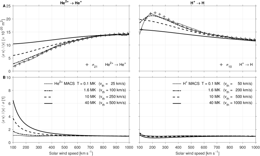
Figure 6: (A). Maxwellian-averaged cross section for single-electron capture by He²⁺ (left) and H⁺ (right) in H₂O. (B). Multiplication factor for the reference non-averaged cross sections. Four solar wind temperatures were used: $T=0.1$ MK, $1.6$ MK, $10$ MK, and $40$ MK, corresponding to varying thermal velocities.

5.3 Maxwellian-averaged ionization cross sections

We present here the MACS for ionization of water vapor by solar wind particles. Because ionization cross sections peak at speeds above $1000$ km s^-1, the increase of the cross sections due to the tail of the Maxwellian distribution will be most important below $400$ km s^-1 for high solar wind temperatures. This is shown in Fig. 7, where Maxwellian-averaged ionization cross sections are calculated for He²⁺ ($\sigma_{22}$) and H⁺ ($\sigma_{11}$).

Cross sections are notably enhanced at typical solar wind speeds ($<1000$ km s^-1), with an increase of more than a factor $10$ at a temperature $T=40\times 10^{6}$ K ($\varv_{\textnormal{th}}=500$ km s^-1) and a solar wind speed of $100$ km s^-1 for He²⁺ (Fig. 7B, left). Correspondingly, the effect is even more drastic for H⁺ (Fig. 7B, right), with a factor $10$ already reached at $400$ km s^-1 solar wind speed for a temperature of $40\times 10^{6}$ K, increasing up to a factor $500$ at $100$ km s^-1. At a solar wind speed of $100$ km s^-1, proton ionization cross sections are multiplied by a factor $16$ and $135$ at the more moderate temperatures of $1.6\times 10^{6}$ K and $10\times 10^{6}$ K, respectively.

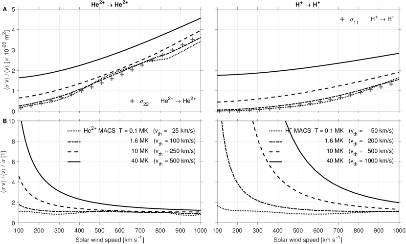
Figure 7: (A). Maxwellian-averaged cross section $\sigma_{\textnormal{MACS}}$ for total ionization of H₂O by impacting He²⁺ (left) and H⁺ (right). (B). Multiplication factor $\gamma$ for the reference non-averaged cross sections, i.e., $\gamma=\sigma_{\textnormal{MACS}}/\sigma$, for He²⁺ (left) and H⁺ (right). Four solar wind temperatures were used: $T=0.1$ MK, $1.6$ MK, $10$ MK, and $40$ MK, corresponding to varying thermal velocities.

5.4 Recommended MACS

Recommended Maxwellian-averaged cross-section bivariate polynomial fits were performed in the 2D solar wind temperature-speed ($T$,$\varv$) space. To constrain the fits, we restricted the temperature range to $0.1-6.4\times 10^{6}$ K for helium particles ($0.025-10\times 10^{6}$ K for hydrogen particles) and set a common solar wind velocity range of $100-800$ km s^-1. We first used a moving average on the calculated MACS to smooth out the sometimes abrupt variations with respect to solar wind speed, which are due to the numerical integration.

Bivariate polynomials of degree $(n,m)$ in temperature (degree $n$) and velocity (degree $m$) can be written for the MACS as $\sigma_{\textnormal{MACS}}(T,\varv)\leavevmode\nobreak\ =\leavevmode\nobreak\ \sum_{i,j}{\leavevmode\nobreak\ p_{ij}\leavevmode\nobreak\ T^{i}\leavevmode\nobreak\ \varv^{j}}\leavevmode\nobreak\ \times\leavevmode\nobreak\ 10^{-22}$ [m²]. Least-absolute-residuals (LAR) bivariate polynomial fits of degree $(4,4)$ or $(4,5)$, with $15$ or $20$ coefficients, respectively, were performed so that the fits could apply to the maximum number of cases without losing in generality and fitting accuracy. The LAR method was preferred to least squares as it gives less weight to extreme values, which, despite smoothing, may appear and are usually connected to the velocity discretization used for the MACS integration. Appendix C presents our recommended bivariate least-squares polynomial fitting coefficients.

Figure 8 displays the comparison in the 2D $(T,\varv)$ plane between the numerically calculated single-electron capture MACS for He²⁺ and H⁺ (as gray contours) and their corresponding polynomial fits (black dotted lines). Good agreement between contours is found for helium and hydrogen, despite the discretization issue around $\varv=500$ km s^-1 for $T<10^{6}$ K. Residuals become important above $800$ km s^-1.

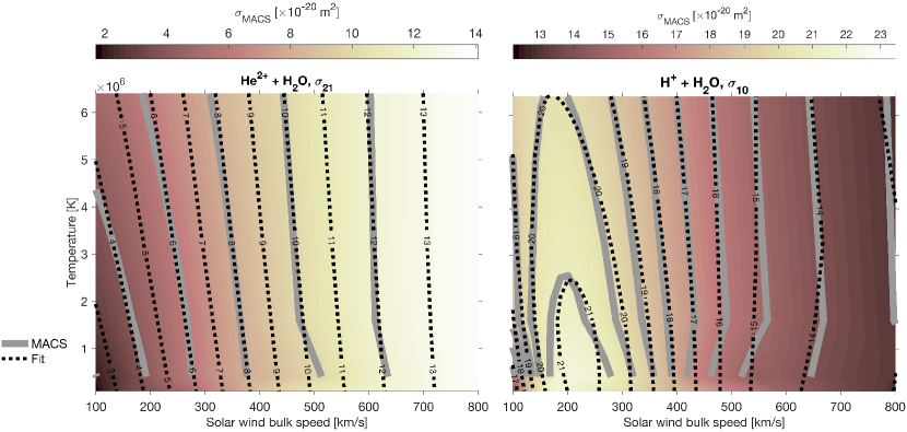
Figure 8: Maxwellian-averaged cross sections in the ($T,\varv$) plane for one-electron capture He${}^{2+}-$H₂O (left) and H${}^{+}-$H₂O (right). Calculated MACS contours are plotted as gray solid lines, and the corresponding fits are shown as black dotted lines.

For helium particles, the error with respect to the calculated charge-changing MACS was kept below $10\%$ on average for fits of degree $(4,4)$, and below $15\%$ for fits of degree $(4,5)$, all within the experimental non-averaged cross-section uncertainties. Because of rapid variations of the cross sections at low solar wind speeds, the fitting error for ionization cross sections is only $<20\%$. For hydrogen particles, the fitting error is correspondingly below $10\%$ for $\sigma_{10}$, $\sigma_{1-1}$ and $\sigma_{01}$, but is about $20\%$ for the other cross sections, including ionization.

6 Summary and conclusions

Figure 9 presents an overview of all fitted charge-changing and ionization cross sections for (He²⁺, He⁺, He) and (H⁺, H, H^-) particles in a water gas, determined from a critical survey of experimental cross sections. The figure illustrates the complexity of ion-neutral interactions because the relative contribution of different reaction channels varies greatly with respect to the collision energy of the projectile. In general, electron capture (charge-exchange) reactions are the prime reactions at low velocities ($<1000$ km/s), whereas stripping, ionization, and/or fragmentation are dominant at higher velocities. We list our results below.

• Helium system. At typical solar wind velocities, the double charge-transfer reaction $\sigma_{20}$ and single-electron capture $\sigma_{10}$ dominate at low impact speeds (below $220$ km s^-1). It is also interesting to note that their main peak is likely situated below $100$ km s^-1, which is the limit of currently available measurements, and which would point to a semi-resonant process taking place. The contribution of double-electron loss $\sigma_{02}$ as a source of He²⁺ is negligible below $1000$ km s^-1. Ionization cross sections peak at solar wind speeds above $4000$ km s^-1 where they are larger than any charge-changing cross section; they are thus expected to play only a minor role in the production of new cometary ions. Electron stripping reactions, especially $\sigma_{01}$ and to a lesser extent $\sigma_{12}$, begin to play an important role at high impact speeds (above $2000$ km s^-1).

• Hydrogen system. Electron capture cross sections ($\sigma_{10}$, $\sigma_{0-1}$) usually dominate for H⁺ and H⁰ species for solar wind speeds below $500$ km s^-1. For H^-, even though the reconstruction of electron stripping cross sections is fraught with uncertainties because of the lack of data, $\sigma_{-10}$ is expected to become the second-most important cross section after $\sigma_{10}$ at typical solar wind speeds $100-1000$ km s^-1. In contrast to the case of He²⁺, double charge-changing reactions (red and green lines) are negligible at typical solar wind speeds; $\sigma_{-11}$ becomes relatively important above $5000$ km s^-1, although it remains about six times lower at its peak than the other sink of H^- ($\sigma_{-10}$). Ionization cross sections, as in the case of the helium system, tend to peak at speeds above $2000$ km s^-1, where they constitute the main source of new ions, only rivalled there by $\sigma_{-10}$ and $\sigma_{01}$.

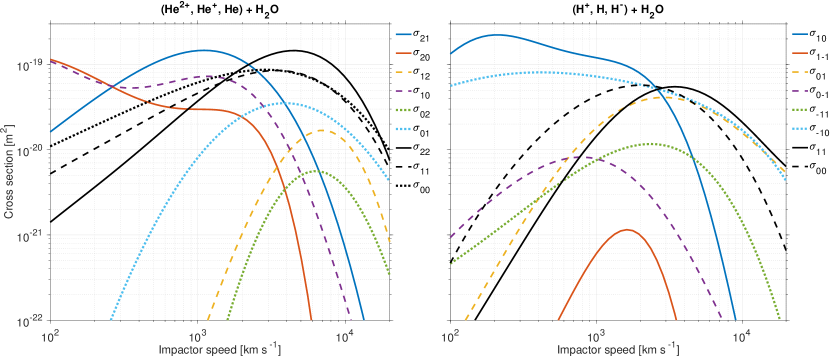
Figure 9: Recommended monochromatic charge-changing and ionization cross sections for (He²⁺, He⁺, He) and (H⁺, H, H^-) in H₂O as a function of impact speed.

The velocity dependence of ion-molecule reactions implies that both the bulk velocity and the temperature of the ions need to be considered. At temperatures above $10$ MK, the high-energy tail of the velocity distribution corresponds to the peak of the single-electron capture by He²⁺ and increases the rate of single-electron capture at low solar wind speeds by almost one order of magnitude. This is also seen for ionization cross sections: MACS are amplified with respect to their parent cross sections for He and even more so for H because of the additive effect of ionization cross sections peaking at high velocities and their rapid decrease at low solar wind speeds. When cross sections peak at low impact speeds, the effect of the distribution becomes small or negligible, as is the case for the single-electron capture by H. This remark also applies to the double- and single-electron captures by He²⁺ and to a lesser extent to the single-electron loss by H^-. This implies that shock structures found around comets and planets, where heating can reach several $10^{6}$ K, may change the balance of ion production and favor processes with cross sections that peak at high energies (ionization and several charge-changing reactions), which were previously thought to be of moderate or negligible importance.

To make the cross-section data more accurate, further experimental studies of helium and hydrogen particles in a H₂O gas are needed for different energy regimes and the following reactions:

• Low-energy regime ($<100$ eV). All $12$ charge-changing reactions for He and H particles in water, and $6$ corresponding ionization cross sections.

• Medium-energy regime ($100-10^{4}$ eV). For He particles, $\sigma_{12}$, $\sigma_{02}$, $\sigma_{01}$, $\sigma_{22}$, and $\sigma_{00}$. For H particles, all cross sections, either charge-exchange or ionization.

• High-energy regime ($10^{4}-10^{5}$ eV). For He particles, $\sigma_{02}$, $\sigma_{01}$ , and $\sigma_{00}$. For H particles, $\sigma_{1-1}$, $\sigma_{-11}$, $\sigma_{-10}$, $\sigma_{00}$, and $\sigma_{-1-1}$.

• Very high-energy regime ($>10^{5}$ eV). For He particles, $\sigma_{12}$, $\sigma_{02}$, $\sigma_{01}$, and ionization cross sections, especially above $500$ keV. For H particles, $\sigma_{-11}$, $\sigma_{-10}$, $\sigma_{00}$, and $\sigma_{-1-1}$.

The critical experimental survey of cross sections presented in this work has multiple applications in astrophysics and space plasma physics (other solar system bodies, H₂O-atmosphere exoplanets), as well as in biophysics as inputs to track-structure models (Uehara et al., 2000; Uehara & Nikjoo, 2002). In parallel with this effort, a corresponding survey of existing theoretical approaches for the calculation of charge-changing and ionization cross sections, with their systematic comparison to experimental datasets, is also needed.

This article is the first part of a study on charge-exchange and ionization efficiency around comets. The second part, presented in Simon Wedlund et al. (2019) (Paper II), develops an analytical formulation of solar wind (H⁺, He²⁺) charge exchange in cometary atmospheres using our recommended set of H₂O charge-exchange cross sections. The third part, presented in Simon Wedlund et al. (2018) (Paper III), applies this analytical model and its inversions to the Rosetta Plasma Consortium datasets, and in doing so, is aimed at quantifying charge-changing reactions and comparing them to other ionization processes during the Rosetta mission to comet 67P.

Appendix A Recommended charge-changing cross sections in H₂O

To facilitate the book-keeping, tables of the recommended fitted monochromatic charge-changing cross sections chosen in this study are given below for the helium (table A) and hydrogen (table A) systems. They are listed between $100$ km s^-1 and $5000$ km s^-1 ($0.05-130$ keV/u) for all processes in numeric form, pending new experimental results. Extrapolations are indicated with an asterisk.

Table 5: Recommended charge-changing cross sections for (He²⁺, He⁺, and He⁰) projectiles colliding with H₂O vapor between $100$ km s^-1 and $5000$ km s^-1 of impact speed.

Speed	Energy	Helium-H2O cross sections
[km s-1]	[keV/amu]	[m2]
		$\sigma_{21}$	$\sigma_{20}$	$\sigma_{12}$	$\sigma_{10}$	$\sigma_{02}$	$\sigma_{01}$
100	0.052	1.62E-20	1.03E-19	2.80E-28∗	1.08E-19∗	9.3E-37∗	8.4E-25∗
150	0.117	2.74E-20	8.46E-20	2.34E-27∗	7.91E-20	8.0E-34∗	7.8E-24∗
200	0.209	3.92E-20	6.65E-20	1.06E-26∗	6.37E-20	6.4E-32∗	3.2E-23∗
250	0.326	5.12E-20	5.40E-20	3.47E-26∗	5.66E-20	1.5E-30∗	8.9E-23∗
300	0.470	6.28E-20	4.58E-20	9.12E-26∗	5.36E-20	1.7E-29∗	1.9E-22∗
350	0.639	7.39E-20	4.02E-20	2.07E-25∗	5.29E-20	1.2E-28∗	3.5E-22
400	0.835	8.43E-20	3.65E-20	4.19E-25∗	5.33E-20	5.7E-28∗	5.8E-22
450	1.06	9.39E-20	3.39E-20	7.81E-25∗	5.45E-20	2.2E-27∗	8.7E-22
500	1.30	1.03E-19	3.21E-20	1.36E-24∗	5.61E-20	6.9E-27∗	1.2E-21
550	1.58	1.10E-19	3.08E-20	2.24E-24∗	5.80E-20	1.9E-26∗	1.7E-21
600	1.88	1.17E-19	3.00E-20	3.52E-24∗	5.99E-20	4.6E-26∗	2.2E-21
700	2.56	1.29E-19	2.90E-20	7.80E-24∗	6.38E-20	2.0E-25∗	3.4E-21
800	3.34	1.37E-19	2.88E-20	1.54E-23∗	6.72E-20	6.7E-25∗	4.8E-21
900	4.23	1.42E-19	2.88E-20	2.77E-23	6.99E-20	1.8E-24∗	6.4E-21
1000	5.22	1.45E-19	2.90E-20	4.64E-23	7.17E-20	4.3E-24∗	8.1E-21
1250	8.16	1.44E-19	2.95E-20	1.34E-22	7.27E-20	2.2E-23∗	1.3E-20
1500	11.7	1.36E-19	2.92E-20	3.05E-22	6.94E-20	7.1E-23∗	1.7E-20
1750	16.0	1.24E-19	2.77E-20	5.89E-22	6.32E-20	1.7E-22∗	2.1E-20
2000	20.9	1.11E-19	2.52E-20	1.01E-21	5.56E-20	3.4E-22∗	2.5E-20
2500	32.6	8.44E-20	1.84E-20	2.29E-21	4.03E-20	9.1E-22∗	3.0E-20
3000	47.0	6.22E-20	1.15E-20	4.12E-21	2.76E-20	1.7E-21∗	3.3E-20
3500	63.9	4.50E-20	6.31E-21	6.31E-21	1.84E-20	2.7E-21∗	3.5E-20
4000	83.5	3.23E-20	3.11E-21	8.65E-21	1.22E-20	3.6E-21	3.5E-20
4500	105.7	2.31E-20	1.40E-21	1.09E-20	8.05E-21	4.4E-21	3.5E-20
5000	130.5	1.66E-20	5.85E-22	1.28E-20	5.34E-21	5.0E-21	3.4E-20

<

25

%

25

-

75

%

>

75

%

.

Table 6: Recommended charge-changing cross sections for (H⁺, H⁰, H^-) projectiles colliding with H₂O vapor between $100$ km s^-1 and $5000$ km s^-1 of impact speed.

Speed	Energy	Hydrogen-H2O cross sections
[km s-1]	[keV/amu]	[m2]
		$\sigma_{10}$	$\sigma_{1-1}$	$\sigma_{01}$	$\sigma_{0-1}$	$\sigma_{-11}$	$\sigma_{-10}$
100	0.052	1.34E-19	4.8E-25	5.17E-23∗	9.4E-22	4.6E-22∗	5.7E-20
150	0.117	2.03E-19	1.9E-24	1.63E-22	1.8E-21	7.5E-22∗	6.8E-20
200	0.209	2.24E-19	4.3E-24	3.80E-22	2.7E-21	1.1E-21∗	7.4E-20
250	0.326	2.19E-19	8.2E-24	7.26E-22	3.6E-21	1.4E-21∗	7.8E-20
300	0.470	2.06E-19	1.4E-23	1.22E-21	4.5E-21	1.8E-21∗	8.0E-20
350	0.639	1.92E-19	2.3E-23	1.86E-21	5.3E-21	2.2E-21∗	8.1E-20
400	0.835	1.79E-19	3.5E-23	2.64E-21	6.0E-21	2.7E-21∗	8.2E-20
450	1.06	1.68E-19	5.1E-23	3.56E-21	6.6E-21	3.1E-21∗	8.2E-20
500	1.30	1.59E-19	7.2E-23	4.60E-21	7.1E-21	3.5E-21∗	8.1E-20
550	1.58	1.52E-19	9.9E-23	5.74E-21	7.4E-21	3.9E-21∗	8.1E-20
600	1.88	1.46E-19	1.3E-22	6.97E-21	7.7E-21	4.4E-21∗	8.0E-20
700	2.56	1.37E-19	2.2E-22	9.63E-21	8.1E-21	5.2E-21	7.8E-20
800	3.34	1.30E-19	3.3E-22	1.24E-20	8.2E-21	6.0E-21	7.7E-20
900	4.23	1.25E-19	4.5E-22	1.53E-20	8.0E-21	6.8E-21	7.5E-20
1000	5.22	1.21E-19	5.9E-22	1.82E-20	7.8E-21	7.5E-21	7.3E-20
1250	8.16	1.11E-19	9.2E-22	2.47E-20	6.8E-21	9.1E-21	6.9E-20
1500	11.7	1.02E-19	1.1E-21	3.02E-20	5.7E-21	1.0E-20	6.5E-20
1750	16.0	9.06E-20	1.1E-21	3.44E-20	4.7E-21	1.1E-20	6.1E-20
2000	20.9	7.91E-20	9.8E-22	3.75E-20	3.8E-21	1.1E-20	5.8E-20
2500	32.6	5.64E-20	5.7E-22	4.08E-20	2.5E-21	1.2E-20	5.3E-20
3000	47.0	3.76E-20	2.6E-22	4.15E-20	1.6E-21	1.1E-20	4.9E-20
3500	63.9	2.39E-20	1.1E-22	4.05E-20	1.1E-21	1.0E-20	4.5E-20
4000	83.5	1.47E-20	4.0E-23	3.87E-20	7.4E-22	9.3E-21	4.1E-20
4500	105.7	8.84E-21	1.5E-23	3.64E-20	5.2E-22	8.2E-21	3.8E-20
5000	130.5	5.27E-21	5.3E-24	3.39E-20	3.7E-22	7.1E-21	3.5E-20

<

25

%

25

-

75

%

>

75

%

.

Appendix B Recommended ionization cross sections in H₂O

We present in Table B our recommended fitted total monochromatic ionization cross sections for helium (He²⁺, He⁺, and He⁰) and hydrogen (H⁺ and H⁰) particles colliding with H₂O. This corresponds to reactions where the impacting species does not change its charge, and is thus complementary for the net production of positive ions to the charge-changing cross sections presented in Appendix A. Ionization cross sections are listed between $100$ km s^-1 and $5000$ km s^-1 ($0.05-130$ keV/u). Extrapolations are indicated with an asterisk.

Table 7: Recommended total ionization cross sections for the (He²⁺, He⁺, He⁰) and (H⁺, H) systems in a H₂O gas between $100$ km s^-1 and $5000$ km s^-1 of impact speed.

Speed	Energy	Helium-H2O			Hydrogen-H2O
[km s-1]	[keV/amu]	[m2]			[$\times 10^{-22}$ m2]
		$\sigma_{22}$	$\sigma_{11}$	$\sigma_{00}$	$\sigma_{11}$	$\sigma_{00}$
100	0.052	1.41E-21∗	5.22E-21∗	1.1E-20∗	3.35E-23∗	4.6E-22∗
150	0.117	2.46E-21∗	7.77E-21∗	1.5E-20∗	1.05E-22∗	1.5E-21
200	0.209	3.63E-21∗	1.03E-20∗	1.9E-20∗	2.34E-22∗	3.2E-21
250	0.326	4.95E-21∗	1.27E-20∗	2.3E-20∗	4.35E-22∗	5.4E-21
300	0.470	6.40E-21∗	1.51E-20∗	2.6E-20∗	7.21E-22∗	7.8E-21
350	0.639	7.99E-21∗	1.76E-20∗	3.0E-20∗	1.10E-21∗	1.1E-20
400	0.835	9.69E-21∗	2.00E-20∗	3.3E-20∗	1.58E-21	1.3E-20
450	1.057	1.15E-20∗	2.23E-20	3.6E-20	2.16E-21	1.6E-20
500	1.305	1.35E-20∗	2.47E-20	3.9E-20	2.85E-21	1.9E-20
550	1.579	1.55E-20∗	2.70E-20	4.2E-20	3.64E-21	2.2E-20
600	1.879	1.76E-20∗	2.93E-20	4.4E-20	4.53E-21	2.5E-20
700	2.558	2.22E-20∗	3.38E-20	4.9E-20	6.59E-21	3.0E-20
800	3.341	2.70E-20∗	3.81E-20	5.4E-20	8.96E-21	3.5E-20
900	4.228	3.20E-20∗	4.22E-20	5.8E-20	1.16E-20	3.9E-20
1000	5.220	3.72E-20∗	4.61E-20	6.2E-20	1.44E-20	4.2E-20
1250	8.156	5.08E-20∗	5.50E-20	6.9E-20	2.19E-20	4.9E-20
1500	11.740	6.44E-20	6.25E-20	7.5E-20	2.93E-20	5.4E-20
1750	15.990	7.76E-20	6.88E-20	8.0E-20	3.60E-20	5.6E-20
2000	20.880	9.00E-20	7.38E-20	8.3E-20	4.18E-20	5.7E-20
2500	32.620	1.11E-19	8.07E-20	8.6E-20	4.99E-20	5.5E-20
3000	46.980	1.27E-19	8.42E-20	8.7E-20	5.40E-20	5.1E-20
3500	63.940	1.38E-19	8.49E-20	8.6E-20	5.50E-20	4.6E-20
4000	83.520	1.44E-19	8.38E-20	8.3E-20	5.39E-20	4.1E-20
4500	105.700	1.46E-19	8.12E-20	8.0E-20	5.16E-20	3.6E-20
5000	130.500	1.44E-19	7.78E-20	7.6E-20	4.85E-20	3.2E-20

<

25

%

25

-

75

%

>

75

%

.

Appendix C Recommended Maxwellian-averaged cross-section fits

Tables C and C present the recommended bivariate polynomial fit coefficients for all $12$ charge-changing cross sections for helium and hydrogen particles in water, as well as the $5$ total ionization cross sections for these two species.

Table 8: Bivariate ($T,\varv$) polynomial fits for Maxwellian-averaged charge-changing and ionization cross sections for (He²⁺, He⁺, and He⁰) projectiles colliding with H₂O vapor. The fits are valid for solar wind speeds $100-800$ km s^-1 and for solar wind temperatures ranging from $100\,000$ K to $6.4\times 10^{6}$ K, unless mentioned otherwise.

Coefficients	Charge-changing cross sections He-H2O						Ionization cross sections He-H2O
	$\sigma_{21}$	$\sigma_{20}$	$\sigma_{12}$	$\sigma_{10}$	$\sigma_{02}$	$\sigma_{01}$	$\sigma_{22}$	$\sigma_{11}$	$\sigma_{00}$
Degree $(n,m)$	(4,4)	(4,5)	(4,4)	(4,5)	(4,4)	(4,4)	(4,4)	(4,4)	(4,4)
$T$ [$\times\ 10^{6}$ K]	$0.1-6.4$	$0.1-1.6$	$0.1-6.4$	$0.1-1.6$	$0.1-6.4$	$0.1-6.4$	$0.1-6.4$	$0.1-6.4$	$0.1-6.4$
$p_{00}$	5.634E+01	1.383E+03	-9.502E-04	1.394E+03	8.597E-04	4.175E-01	4.810E+00	2.141E+01	5.216E+01
$p_{10}$	5.115E-05	-5.115E-04	-5.163E-10	-4.580E-04	-1.461E-10	-5.627E-07	7.017E-06	1.967E-05	3.431E-05
$p_{01}$	1.440E-03	-4.620E-03	1.831E-08	-5.801E-03	-1.421E-08	2.190E-07	5.522E-05	2.820E-04	5.829E-04
$p_{20}$	-1.716E-12	1.324E-10	1.334E-16	1.167E-10	-4.114E-18	1.798E-13	-9.003E-13	-3.032E-12	-5.332E-12
$p_{11}$	-8.517E-11	2.312E-09	4.072E-15	2.570E-09	2.078E-15	4.777E-12	7.435E-12	-2.469E-11	-6.996E-11
$p_{02}$	2.829E-09	5.499E-09	-8.826E-14	1.341E-08	7.786E-14	-5.953E-11	5.125E-10	6.901E-10	6.584E-10
$p_{30}$	3.962E-20	-1.750E-17	-2.320E-23	-1.461E-17	2.075E-24	-2.328E-20	1.592E-19	4.838E-19	7.900E-19
$p_{21}$	1.890E-18	-4.747E-16	8.743E-23	-4.766E-16	-2.851E-23	-5.152E-19	-1.088E-18	2.333E-19	3.801E-18
$p_{12}$	1.859E-17	-3.409E-15	-1.236E-20	-4.711E-15	-8.113E-21	-2.344E-18	-2.587E-17	5.518E-18	5.026E-17
$p_{03}$	-4.679E-15	1.131E-15	1.945E-20	-1.248E-14	-1.747E-19	3.069E-16	-1.541E-16	-8.664E-16	-1.216E-15
$p_{40}$	-3.331E-28	8.607E-25	2.098E-30	6.914E-25	-8.472E-32	1.055E-27	-9.403E-27	-2.733E-26	-4.221E-26
$p_{31}$	-2.015E-26	4.745E-23	-5.493E-29	4.394E-23	-6.737E-30	4.139E-26	4.004E-26	-5.024E-26	-2.637E-25
$p_{22}$	-4.579E-25	4.740E-22	8.608E-28	5.430E-22	1.719E-28	-6.375E-26	7.008E-25	6.289E-25	-7.978E-25
$p_{13}$	1.647E-23	1.909E-21	2.855E-26	3.563E-21	9.351E-27	1.438E-24	1.882E-23	6.757E-24	-6.629E-24
$p_{04}$	1.810E-21	-5.883E-21	4.557E-25	4.205E-21	1.396E-25	-1.808E-22	-7.139E-23	3.258E-22	5.335E-22
$p_{41}$	$-$	-1.720E-30	$-$	-1.513E-30	$-$	$-$	$-$	$-$	$-$
$p_{32}$	$-$	-2.304E-29	$-$	-2.339E-29	$-$	$-$	$-$	$-$	$-$
$p_{23}$	$-$	-1.472E-28	$-$	-1.980E-28	$-$	$-$	$-$	$-$	$-$
$p_{14}$	$-$	-2.730E-28	$-$	-9.401E-28	$-$	$-$	$-$	$-$	$-$
$p_{05}$	$-$	2.774E-27	$-$	3.938E-30	$-$	$-$	$-$	$-$	$-$

<

25

%

25-

75

%

>75

%

.

Table 9: Bivariate ($T,\varv$) polynomial fits for Maxwellian-averaged charge-changing and ionization cross sections for (H⁺, H⁰, and H^-) projectiles colliding with H₂O vapor. The fits are valid for solar wind speeds $100-800$ km s^-1 and for solar wind temperatures ranging from $25\,000$ K to $10\times 10^{6}$ K, unless mentioned otherwise.

Coefficients	Charge-changing cross sections H-H2O						Ionization cross sections H-H2O
	$\sigma_{10}$	$\sigma_{1-1}$	$\sigma_{01}$	$\sigma_{0-1}$	$\sigma_{-11}$	$\sigma_{-10}$	$\sigma_{11}$	$\sigma_{00}$
Degree $(n,m)$	(4,5)	(4,4)	(4,4)	(4,5)	(4,4)	(4,5)	(4,4)	(4,4)
$T$ [$\times\ 10^{6}$ K]	$0.025-10$	$0.025-1.6$	$0.025-10$	$0.025-1.6$	$0.025-10$	$0.025-10$	$0.025-10$	$0.025-10$
$p_{00}$	6.151E+01	-3.085E-02	-2.149E+00	1.899E+00	1.679E+00	5.445E+02	-9.696E-01	-1.212E+01
$p_{10}$	3.886E-04	2.826E-08	5.952E-06	2.109E-05	6.312E-06	1.003E-04	3.118E-06	3.543E-05
$p_{01}$	2.331E-02	5.110E-07	-1.595E-05	5.904E-05	2.749E-05	1.249E-03	-6.480E-06	7.489E-05
$p_{20}$	-5.076E-11	3.080E-14	7.320E-14	-4.450E-12	-7.040E-13	-2.007E-11	2.893E-13	-3.656E-12
$p_{11}$	-3.137E-09	1.077E-13	3.381E-12	-4.133E-11	-6.877E-12	-4.151E-10	3.639E-12	-2.506E-11
$p_{02}$	-9.085E-08	-3.405E-12	2.546E-10	5.611E-10	1.342E-10	-1.057E-09	9.705E-11	1.133E-09
$p_{30}$	4.472E-18	-3.201E-21	-4.963E-21	4.808E-19	6.839E-20	1.948E-18	-2.719E-20	3.602E-19
$p_{21}$	2.028E-16	-1.941E-20	-1.956E-19	1.057E-17	6.270E-19	6.146E-17	-3.573E-19	2.821E-18
$p_{12}$	8.870E-15	8.670E-19	-9.357E-19	-3.972E-17	1.168E-18	4.984E-16	6.289E-18	-3.051E-17
$p_{03}$	1.455E-13	1.389E-17	-2.668E-17	-1.115E-15	-1.373E-16	-2.555E-15	1.024E-16	-1.098E-15
$p_{40}$	-1.530E-25	1.186E-28	1.190E-28	-1.797E-26	-2.416E-27	-6.820E-26	9.413E-28	-1.268E-26
$p_{31}$	-1.172E-23	9.531E-28	7.201E-27	-1.087E-24	-2.645E-26	-4.878E-24	1.426E-26	-1.379E-25
$p_{22}$	-2.677E-22	1.022E-27	7.523E-26	-1.775E-24	-1.521E-25	-4.111E-23	1.166E-25	-2.291E-25
$p_{13}$	-1.050E-20	-9.332E-25	-6.307E-24	8.836E-23	4.486E-25	-2.427E-22	-9.814E-24	2.507E-23
$p_{04}$	-1.030E-19	-4.447E-24	-1.437E-23	7.177E-22	5.356E-23	4.788E-21	-3.734E-23	3.310E-22
$p_{41}$	2.810E-31	$-$	$-$	3.524E-32	$-$	1.357E-31	$-$	$-$
$p_{32}$	6.353E-30	$-$	$-$	2.508E-31	$-$	1.766E-30	$-$	$-$
$p_{23}$	1.181E-28	$-$	$-$	-2.311E-30	$-$	5.386E-30	$-$	$-$
$p_{14}$	4.464E-27	$-$	$-$	-3.188E-29	$-$	4.929E-29	$-$	$-$
$p_{05}$	2.572E-26	$-$	$-$	-1.419E-28	$-$	-2.276E-27	$-$	$-$

<

25

%

25-

75

%

>75

%

.