On closed oriented surfaces in the 3-sphere

Abstract.

In this paper we study embeddings of oriented connected closed surfaces in $\mathbb{S}^{3}$. We define a complete invariant, the fundamental span, for such embeddings, generalizing the notion of the peripheral system of a knot group. From the fundamental span, several computable invariants are derived and employed to study handlebody knots, bi-knotted surfaces, and chirality of knots. These invariants are capable to distinguish inequivalent handlebody knots and bi-knotted surfaces with homeomorphic complements. Particularly, we obtain an alternative proof of the inequivalence of Ishii et al.’s handlebody knots $5_{1}$ and $6_{4}$, and also construct an infinite family of pairs of inequivalent bi-knotted surfaces with homeomorphic complements. An interpretation of Fox’s invariant in terms of the fundamental span is discussed and used to show $9_{42}$ and $10_{71}$ in the Rolfsen knot table are chiral; their chirality is known to be undetectable by the Jones and HOMFLY-PT polynomials.

1. Introduction

By the Gordon-Luecke theorem [12] and Waldhausen’s theorem [38], the knot type of a knot $K\subset\mathbb{S}^{3}$ is determined, up to mirror image, by its knot group $G_{K}$ and peripheral system. More precisely, the peripheral system is the subgroup of $G_{K}$ generated by elements represented by a meridian $m$ and a preferred longitude $l$ through a base point. If furthermore, we require $m$ and $l$ are positively oriented with respect to the orientation of $\mathbb{S}^{3}$, then the knot group together with the conjugacy classes of the elements $[m]$, $[l]$ completely determines the knot type of $K\subset\mathbb{S}^{3}$.

Taking a tubular neighborhood of a knot, one can view a knot as an embedded solid torus in $\mathbb{S}^{3}$. The solid torus inherits a natural orientation from $\mathbb{S}^{3}$, and induces an orientation on its boundary. In this way, a knot can be thought of as an embedded oriented surface in $\mathbb{S}^{3}$ [34]. The assignment from the category of knots to the category of oriented connected closed surfaces in $\mathbb{S}^{3}$ is one-to-one, and therefore to distinguish the knot types of two knots amounts to determining whether the associated embedded oriented surfaces are ambient isotopic. The aim of this paper is to construct a complete invariant for oriented connected closed surfaces of arbitrary genus smoothly embedded in $\mathbb{S}^{3}$, generalizing the knot group with its peripheral system, and examine the topology of connected closed surfaces in $\mathbb{S}^{3}$ via computable invairants derived therefrom.

Any oriented connected closed surface $\Sigma$ in $\mathbb{S}^{3}$ gives rise to an oriented $3$-dimensional submanifold $E$ in $\mathbb{S}^{3}$ which is the closure of the connected component in $\mathbb{S}^{3}\setminus E$ satisfying $\partial E=\Sigma$ (i.e. with a compatible orientation). Conversely, given any connected $3$-dimensional submanifold with connected boundary $E\subset\mathbb{S}^{3}$, $\partial E$ is an oriented connected closed surface in $\mathbb{S}^{3}$. In particular, the notion of oriented connected closed surfaces in $\mathbb{S}^{3}$ generalizes embeddings of handlebodies in $\mathbb{S}^{3}$, namely handlebody knots. An oriented connected closed surfaces $\Sigma$ in $\mathbb{S}^{3}$ can be viewed as a partition of $\mathbb{S}^{3}$, in which we let $E$ be the “inside” and the “outside” is the closure $F$ of the complement of $E$. We denote by the triplet $(E,\Sigma,F)$ such a partition. For instance, given a knot $K$, $E$ is a tubular neighborhood of $K$.

On the other hand, if no prescribed orientation of $\Sigma$ is given, there is no way to distinguish between $E$ and $F$. Embeddings of unoriented surfaces in $\mathbb{S}^{3}$ are studied, for example, in [9], [14]. In the genus-one case, it is equivalent to knots in $\mathbb{S}^{3}$. More generally, an unoriented surface $\Sigma$ of genus $g$ in $\mathbb{S}^{3}$ with the closure of one component of $\mathbb{S}^{3}\setminus\Sigma$ a handlebody is equivalent to a handlebody knot. There is an obvious forgetful functor from the category of oriented connected surfaces in $\mathbb{S}^{3}$ to the category of connected surfaces in $\mathbb{S}^{3}$ by ignoring the distinction between the inside and outside (see Diagram 2.1).

The denomination “inside” and “outside” is borrowed from the setting of [2], where the ambient space is $\mathbb{R}^{3}$, topologically equivalent to $\mathbb{S}^{3}$ with “the point at infinity” $\infty$ removed, and $E$, a $3$-submanifold with (a not necessarily connected boundary) of $\mathbb{R}^{3}$, is called a scene. In topology, studies from this point of view can be found in [35], [36]. This motivates our choice of the name “scene” for the triplet $(E,\Sigma,F)$ (Definition 2.1).

Having an infinite point allows us to orient $\Sigma$ naturally and thus distinguish between $E$ and $F$. Discussion from this point of view can be found in [3]. Apart from this, $E$ and $F$ are treated equally in the sense that they play an equally important role in the triplet $(E,\Sigma,F)$.

In this paper we confine ourselves to the case of connected scenes $(E,\Sigma,F)$ (i.e. $\Sigma$ is connected). For each component in $(E,\Sigma,F)$, we consider its fundamental group, and the three fundamental groups are interrelated via the homomorphisms induced by the inclusions $i_{E}:\Sigma\to E$, $i_{F}:\Sigma\to F$. The orientation information can be captured by taken into account the intersection form on the first homology group $H_{1}(\Sigma)$ of $\Sigma$. In the case of knots, the fundamental group of $F$ corresponds to the knot group, whereas the kernel of $\pi_{1}(\Sigma,\ast)\to\pi_{1}(E,\ast)$ and the image of $\pi_{1}(\Sigma,\ast)\to\pi_{1}(F,\ast)$, $\ast\in\Sigma$, along with the intersection form on $H_{1}(\Sigma)$ give the peripheral system.

This leads to our definition of a group span with pairing (Definition 3.1), which is an ordered triplet of groups $(G,\Upsilon,H)$ along with two connecting homomorphisms $i_{G}:\Upsilon\rightarrow G$, $i_{H}:\Upsilon\rightarrow H$ and a pairing on the abelianization of $\Upsilon$. A connected scene $\mathcal{S}=(E,\Sigma,F)$ induces a natural group span with pairing, called the fundamental span of $\mathcal{S}$, $(\pi_{1}(E,\ast),\pi_{1}(\Sigma,\ast),\pi_{1}(F,\ast),{i_{E}}_{\ast},{i_{F}}_{\ast},d)$, where $\ast\in\Sigma$ is a base point, $\pi_{1}(\cdot)$ is the fundamental group, and $d$ is the intersection form on the first integral homology group $H_{1}(\Sigma,\mathbb{Z})$ of $\Sigma$ (Definition 3.3). One of the main results in the paper is Theorem 3.2, where we show that the fundamental span is a complete invariant for connected scenes, up to ambient isotopy.

We remark that Theorem 3.2 does not imply the Gordon-Luecke theorem [12]. Indeed the Gordon-Luecke theorem along with Waldhausen’s theorem imply a stronger version of Theorem 3.2 in the case of knots: given two embedded tori $E\subset\mathbb{S}^{3}$ and $E^{\prime}\subset\mathbb{S}^{3}$, suppose there are isomorphisms connecting $\phi_{F}:\pi_{1}(F,\ast)\rightarrow\pi_{1}(F^{\prime},\ast^{\prime})$ and $\phi_{\Sigma}:\pi_{1}(\Sigma,\ast)\rightarrow\pi_{1}(\Sigma^{\prime},\ast^{\prime})$ such that ${i_{F}^{\prime}}_{\ast}\circ\phi_{\Sigma}=\phi_{\Sigma}\circ{i_{F}}_{\ast}$, with $\phi_{\Sigma}$ preserving the intersection forms on $H_{1}(\Sigma,\mathbb{Z})$ and $H_{1}(\Sigma^{\prime},\mathbb{Z})$. Then the two solid tori in $\mathbb{S}^{3}$ are equivalent. On the other hand, in order to obtain a complete invariant for oriented surfaces of genus larger than one, it is necessary to take into account the information hidden in the induced homomorphism ${i_{E}}_{\ast}:\pi_{1}(\Sigma,\ast)\rightarrow\pi_{1}(E,\ast)$, given there are infinite many handlebody knots with homeomorphic complements.

Having a complete invariant does not close the classification problem of knots. In fact, the problem of distinguishing two finite presentations of groups, up to isomorphism, is in general unsolvable in the sense that there is no algorithm that always give an answer in a finite time [6]. Proving isomorphism is generally done by finding a sequence of Tietze moves that connects the two presentations, whereas proving that two presentations describe non-isomorphic groups often requires computable invariants, such as the Alexander invariant. Another aim of the paper is to construct strong, computable invariants out of the fundamental span, and particularly those able to differentiate connected scenes with homeomorphic components.

The first invariant applies primarily for handlebody knots, and it inspired by Fox’s proof [11] of inequivalence of the square knot and granny knot, and Riely’s work [29] and Kitano and Suzuki’s work [16] on homomorphisms from a knot group to a finite group,

To construct the invariant, we consider the subgroup ${i_{F}}_{\ast}(\operatorname{Ker}({i_{E}}_{\ast}))$, which is the image of the kernel of

$${i_{E}}_{\ast}:\pi_{1}(\Sigma,\ast)\rightarrow\pi_{1}(E,\ast)$$ (1.1)

in $\pi_{1}(F,\ast)$ under

$${i_{F}}_{\ast}:\pi_{1}(\Sigma,\ast)\rightarrow\pi_{1}(F,\ast).$$

Consider also the surjective homomorphisms from $\pi_{1}(F,\ast)$ to a finite group $G$ that are not surjective after being precomposed with ${i_{F}}_{*}$. Such homomorphisms are called proper homomorphisms (Definition 5.1). Then the set of the images of the subgroup ${i_{F}}_{\ast}(\operatorname{Ker}({i_{E}}_{\ast}))$ in $G$ under proper homomorphisms up to automorphisms of $G$ is an invariant of the connected scene $\mathcal{S}=(E,\Sigma,F)$. The invariant takes value in the set of finite sets of subgroups of $G$, up to automorphisms of $G$, and is called the $G$-image of meridians of $\mathcal{S}$ (Definition 5.2) since the kernel of (1.1) can be identified with the normal closure of meridians of $E$. It turns out that the $G$-image of meridians (Definition 5.2) can see subtle difference between handlebody knots. To investigate this invariant, we generalize Motto’s and Lee-Lee’s constructions [25], [18] to generate a wide array of inequivalent handlebody knots with homeomorphic complements; computing the $G$-image of meridians for these examples shows that it is capable to distinguish many of such handlebody knots.

Inequivalent handlebody knots with homeomorphic complements are first discovered by Motto [25] with a geometric argument; in the end of his paper he asks for a computable way to detect such handlebody knots. The computable invariant devised here partially answers his challenge. On the other hand, due to the finiteness of the group $G$, our invariant cannot distinguish an infinite family of such handlebody knots as Motto’s approach did.

Contrary to knots, inequivalent handlebody knots with homeomorphic complements abound. $(5_{1},6_{4})$ and $(5_{2},6_{13})$ in Ishii et al.’s handlebody knot table [15], are two such pairs. The inequivalence of $5_{1}$ and $6_{4}$ (resp. $5_{2}$ and $6_{13}$) is proved by a geometric means in [18]. Our computational method shows that the $A_{5}$-image of meridians can also see the difference between $5_{1}$ and $6_{2}$, However, it fails to differentiate $5_{2}$ from $6_{13}$. Via the $A_{5}$-image of meridians, we further identify two $7$ crossings handlebody knots whose complements are homeomorphic to the complements of some handlebody knots in Ishii et al.’s handlebody table.

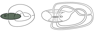
Figure 1.1. Handcuff graph with a $2$-cell $D$ and the associated handlebody knot with a transverse disk.

Figure 1.2. Performing the satellite construction along a knot $K$ w.r.t. a transverse disk $D$.

To investigate the usefulness of the fundamental span in the case of bi-knotted scenes, that is neither $E$ nor $F$ a $3$-handlebody, we introduce the notion of transverse disks of a handlebody knot (Definitions 4.1 and 4.3) and the satellite construction along a knot with respect to (w.r.t. hereafter) a transverse disk. For instance, every handcuff graph in $\mathbb{S}^{3}$ with at least one of its two circles unknotted in $\mathbb{S}^{3}$ admits a natural transverse disk (Fig. 1.1).

Performing the satellite construction amounts to replacing a $3$-ball neighborhood of the transverse disk by a $3$-ball with knotted tubes inside (Fig. 1.2).

The satellite construction gives an ample supply of bi-knotted scenes derived from handlebody knots. In Ishii et al.’s handlebody knot table, there are $10$ handcuff graph diagrams, each of which has two unknotted circles in $\mathbb{S}^{3}$, and hence admits two natural transverse disks. A question thus arises as to whether performing the satellite construction w.r.t. the two transverse disks results in equivalent bi-knotted scenes. In some cases, the equivalence is obvious, while in the other cases, proving or disproving the equivalence between them could be challenging. We derive an invariant of irreducible handlebody knots with a transverse disk from the fundamental span, and use it to show that $5_{1}$, $6_{1}$ and $6_{11}$ are the only three among the ten handcuff diagrams, where performing the satellite construction w.r.t. associated disks yields inequivalent bi-knotted scenes.

Lastly, we examine the role of the intersection form in the fundamental span, a crucial ingredient in discerning the chirality of a connected scene. We demonstrate this by translating Fox’s argument [11] into an invariant in terms of the fundamental span, and via the invariant, we determine the chirality of $9_{42}$ and $10_{71}$ in the Rolfsen knot table; their chirality is known to be undetectable by any known knot polynomials. In [28], Chern-Simons invariants are employed to determine their chirality; another approach via the determinant of a knot is discussed in [8].

The paper is organized as follows: In Section 2 we introduce the notion of scene and equivalence of scenes. In Section 3, we construct the assignment from the category of connected scenes to the category of group spans with pairing and show the assignment is one-to-one. Section 4 discusses constructions that generate connected scenes with homeomorphic components. We produce several examples and study their properties. Invariants of group spans with pairing defined in terms of homomorphisms of $\pi_{1}(F,\ast)$ into a given finite group are introduced in Section 5; they are used in subsection 5.4 to prove statements given in Section 4.

2. Scenes and scenes equivalence

Definition 2.1 (Scene).

A scene in $\mathbb{S}^{3}$ is an ordered triplet $\mathcal{S}=(E,\Sigma,F)$ of oriented manifolds in $\mathbb{S}^{3}$ in the smooth category such that $E$ and $F$ are $3$-manifolds with $E\cup F=\mathbb{S}^{3}$ and $E\cap F=\Sigma$, where $\Sigma$ is a closed oriented surface with $\Sigma=\partial E=-\partial F$.

Definition 2.2 (Equivalence of scenes).

Two scenes $\mathcal{S}=(E,\Sigma,F)$ and $\mathcal{S}^{\prime}=(E^{\prime},\Sigma^{\prime},F^{\prime})$ (or two embeddings $E\hookrightarrow\mathbb{S}^{3}$ and $E^{\prime}\hookrightarrow\mathbb{S}^{3}$) are equivalent, if there exists an ambient isotopy $\Phi_{t}:\mathbb{S}^{3}\rightarrow\mathbb{S}^{3}$ such that $\Phi_{0}=\textrm{id}$ and $\Phi_{1}(E)=E^{\prime}$

The definition implies automatically $\Phi_{1}(\Sigma)=\Sigma^{\prime}$ and $\Phi_{1}(F)=F^{\prime}$.

Remark 2.1.

$\Phi_{1}$ is an orientation-preserving self-diffeomorphism of $\mathbb{S}^{3}$ sending $E$ to $E^{\prime}$, and conversely, any orientation-preserving self-diffeomorphism of $\mathbb{S}^{3}$ sending $E$ to $E^{\prime}$ is connected to the identity via an ambient isotopy [4].

Definition 2.3 (Connected scene, genus).

A scene $\mathcal{S}=(E,\Sigma,F)$ is connected if $\Sigma$ is connected. The genus of a connected scene $\mathcal{S}=(E,\Sigma,F)$ is the genus of the surface $\Sigma$.

A connected scene has connected inside $E$ and outside $F$ as $\Sigma=\partial E=-\partial F$.

In this paper, we shall restrict ourselves to connected scenes. Relations with other embedded objects in $\mathbb{S}^{3}$, as discussed in the introduction, are summarized in the diagram below ($\rightarrowtail$ stands for an injection of categories and $\twoheadrightarrow$ for a surjection):

(2.1)

In view of the diagram, we call a connected scene a knot if $E$ is a solid torus and call it a handlebody knot if $E$ is a $3$-handlebody of genus $g\geq 1$.

Definition 2.4 (Trivial scene).

A connected scene $(E,\Sigma,F)$ is trivial if both $E$ and $F$ are $3$-handlebodies.

Note that, by [37, Satz $3.1$], the Heegaard splitting of $\mathbb{S}^{3}$ of genus $g$ is unique, for every $g\geq 0$, namely the standard one. Hence, every two trivial scenes of the same genus are ambient isotopic. We use the symbol $H_{g}$ to denote a handlebody of genus $g$ and $\Sigma_{g}$ a surface of genus $g$. We drop $g$ when there is no risk of confusion.

Definition 2.5 (Bi-knotted scene).

A bi-knotted scene is a connected scene $(E,\Sigma,F)$ with neither $E$ nor $F$ a $3$-handlebody.

To understand the relation between connected scenes (or equivalently oriented connected closed surfaces in $\mathbb{S}^{3}$) and connected closed surfaces in $\mathbb{S}^{3}$ (mapping p in Diagram (2.1) above) we observe that, given a connected surface $\Sigma$ in $\mathbb{S}^{3}$, if the connected components $V_{1}$ and $V_{2}$ of $\mathbb{S}^{3}\setminus\Sigma$ are not homeomorphic, then the preimage of the surface in $\mathbb{S}^{3}$ under p contains precisely two elements—one regards $V_{1}$ as, say, the “inside” and $V_{2}$ as the “outside”.

If $V_{1}$ and $V_{2}$ are homeomorphic, the situation is subtler. For the sake of convenience, we give the following definition.

Definition 2.6 (Symmetric scene).

A connected scene $(V,\Sigma,W)$ is symmetric if $V$ and $W$ are homeomorphic.

Definition 2.7 (Swappable/unswappable scene).

A symmetric scene $(V,\Sigma,W)$ is swappable (resp. unswappable) if it is equivalent (resp. inequivalent) to $(W,-\Sigma,V)$.

In the case of genus one, the only symmetric scene is the trivial scene and it is swappable. In the case of genus two, by [36, Theorem $1$], every symmetric scene $(V,\Sigma_{2},W)$ must have $V$ (resp. $W$) homeomorphic to the boundary connected sum of a solid torus $H_{1}$ and the complement of an open tubular neighborhood of a knot $K_{V}$ (resp. $K_{W}$). Thus, by the Gordon-Luecke theorem [12] and [34, Corollary $3.4$], the knots $K_{V}$ and $K_{W}$ are equivalent, up to mirror image. Therefore, a symmetric scene $(V,\Sigma_{2},W)$ of genus $2$ is unswappable if and only if $K_{V}$ and $K_{W}$ are chiral knots and mirror images to each other. Using a corollary of Waldhausen’s theorem [35, Theorem $3$], we obtain the following theorem:

Theorem 2.1.

There exist unswappable symmetric connected scenes of genus $g$, for any $g>1$.

Definition 2.8 (Sum operation).

Given two connected scenes $\mathcal{S}=(E,\Sigma,F)$ and $\mathcal{S}^{\prime}=(E^{\prime},\Sigma^{\prime},F^{\prime})$, their connected sum $\mathcal{S}\#\mathcal{S}^{\prime}$ is a connected scene given by removing a point $p\in\Sigma$ and a point $p^{\prime}\in\Sigma^{\prime}$ and glue them together via an orientation-reversing diffeomorphism

$$(B_{p}\cap\Sigma,B_{p})\simeq(\mathbb{S}^{1},\mathbb{S}^{2})\times(0,1) \rightarrow(B_{p^{\prime}}\cap\Sigma^{\prime},B_{p^{\prime}})\simeq(\mathbb{S}^{1},\mathbb{S}^{2})\times(0,1)$$

$$(x,t) \rightarrow(x,1-t),$$

where $B_{p}$ (resp. $B_{p^{\prime}}$) is a $3$-ball neighborhood of $p$ (resp. $p^{\prime}$) in $\mathbb{S}^{3}$ with $p$ (resp. $p^{\prime}$) removed. The first and last orientation-preserving diffeomorphism identify $B_{p}$ and $B_{p}^{\prime}$ with a unit $3$-ball, respectively. The components of $\mathcal{S}\#\mathcal{S}^{\prime}$ are denoted by $(E\#E^{\prime},\Sigma\#\Sigma^{\prime},F\#F^{\prime})$.

The sum operation is associative and commutative.

Given a connected scene $\mathcal{S}$, if it is equivalent to the connected sum of connected scenes $\mathcal{S}_{i}$, $i=1,...n$, then we say $\mathcal{S}_{1}\#\mathcal{S}_{2}\#...\#\mathcal{S}_{n}$ is a decomposition of $\mathcal{S}$.

Definition 2.9 (Prime scenes).

A connected scene $\mathcal{S}$ is prime if its genus is larger than $0$ and admits no decomposition $\mathcal{S}=\mathcal{S}_{1}\#\mathcal{S}_{2}$ with both $\mathcal{S}_{1}$ and $\mathcal{S}_{2}$ non-trivial. A decomposition $\mathcal{S}\simeq\mathcal{S}_{1}\#\mathcal{S}_{2}\#...\#\mathcal{S}_{n}$ is prime if $\mathcal{S}_{i}$ is prime, $i=1,...,n$.

Note that our prime handlebody knots are called irreducible handlebody knots in [15]. The notation chosen here is consistent with that in [34], [36] and in knot theory. In particular, a scene $\mathcal{S}$ is prime if and only if $p(\mathcal{S})$ regarded as an unoriented surface in $\mathbb{S}^{3}$, is prime. On the other hand, the notions of prime $\theta$-curves and handcuff graphs in [23], [24] have different meanings.

The examples of unswappable scenes given above are non-prime. In fact, there is no unswappable prime scene with genus less than $3$. In Section 4.2, we give a construction of unswappable prime scenes of genus $3$, as an application of the existence of inequivalent handlebody knots with homeomorphic complements, and prove the following result:

Theorem 2.2.

There exist infinitely many unswappable prime scenes of genus $3$.

3. Fundamental structure for connected scenes

Given a connected scene $\mathcal{S}=(E,\Sigma,F)$ and a base point $\ast\in\Sigma$, the fundamental groups $\pi_{1}(E,\ast)$, $\pi_{1}(\Sigma,\ast)$, and $\pi_{1}(F,\ast)$ are related to each other via the homomorphisms ${i_{E}}_{*}$ and ${i_{F}}_{*}$ induced by the inclusions $i_{E}:\Sigma\to E$ and $i_{F}:\Sigma\to F$, respectively. In general, ${i_{E}}_{*}$ and ${i_{F}}_{*}$ are neither injective nor surjective.

The following unknotting theorem is a corollary of [13, Theorem $5.2$].

Proposition 3.1.

Let $\mathcal{S}=(E,\Sigma,F)$ be a connected scene and $\ast\in\Sigma$ a basepoint. Then $\mathcal{S}$ is trivial if and only if $\pi_{1}(E,\ast)$ and $\pi_{1}(F,\ast)$ are free groups.

Proof.

[13, Theorem $5.2$] asserts that a prime $3$-manifold with the fundamental group a free group is either a $S^{2}$ bundle over $S^{1}$ or a $3$-ball with some $1$-handles attached to its boundary.

Now, since $\Sigma$ is connected, its complements $E$ and $F$ must be irreducible $3$-manifolds, and hence, $\pi_{2}(E,\ast)$ and $\pi_{2}(F,\ast)$ are trivial by the sphere theorem. That implies $E$ (resp. $F$) cannot be a $S^{2}$-bundle over $S^{1}$. On the other hand, any $3$-manifold in $S^{3}$ is orientable, so $E$ (resp. $F$) must be a $3$-handlebody. ∎

The topological type of a connected scene $\mathcal{S}=(E,\Sigma,F)$ is not determined solely by the fundamental groups of $E$ and $F$; there are inequivalent connected scenes with homeomorphic outsides and insides [25], [18]. To distinguish such connected scenes, additional structures need to be taken into account.

To this aim, we introduce the notion of a fundamental span, which is an analog of a knot group with the peripheral system; the following definitions describes the algebraic universe where fundamental spans live.

Definition 3.1 (Group span with pairing).

A group span with pairing is an ordered triplet of groups $(G,\Upsilon,H)$ along with two connecting homomorphisms $i_{G}:\Upsilon\rightarrow G$ and $i_{H}:\Upsilon\rightarrow H$ and a non-degenerate pairing $d:\Upsilon/[\Upsilon,\Upsilon]\times\Upsilon/[\Upsilon,\Upsilon]\rightarrow\mathbb{Z}$, where $[A,A]$ denotes the commutator subgroup of the group $A$.

Definition 3.2 (Equivalence of group spans with pairing).

Two group spans with pairing

$$(G,\Upsilon,H,i_{G},i_{H},d),\qquad(G^{\prime},\Upsilon^{\prime},H^{\prime},i_{G^{\prime}},i_{H^{\prime}},d^{\prime})$$

are equivalent if there are isomorphisms $G\rightarrow G^{\prime}$, $\Upsilon\rightarrow\Upsilon^{\prime}$, and $H\rightarrow H^{\prime}$ such that the diagram

commutes and the isomorphism $\Upsilon\rightarrow\Upsilon^{\prime}$ preserves the pairings $d$ and $d^{\prime}$.

Given a connected scene $\mathcal{S}=(E,\Sigma,F)$ and a base point $\ast\in\Sigma$, the fundamental group functor $\pi_{1}(-)$ gives a group span with pairing

$$(\pi_{1}(E,\ast),\pi_{1}(\Sigma,\ast),\pi_{1}(F,\ast),{i_{E}}_{*},{i_{F}}_{*},d),$$ (3.1)

where $d$ is the intersection form on $H_{1}(\Sigma,\mathbb{Z})$ given by the orientation of $\Sigma$. Notice that using different base points results in equivalent group spans with pairing; thus the equivalence class of (3.1) is independent of the choice of a base point.

Definition 3.3 (Fundamental span).

Given a connected scene $\mathcal{S}=(E,\Sigma,F)$, the equivalence class of $(\pi_{1}(E,\ast),\pi_{1}(\Sigma,\ast),\pi_{1}(F,\ast),{i_{E}}_{*},{i_{F}}_{*},d)$ is called the fundamental span of $\mathcal{S}$, and is denoted by $\mathcal{F}(\mathcal{S})$.

Any (base point preserving) equivalence between (based) connected scenes induces equivalent group spans with pairing; thus, $\mathcal{F}(\cdot)$ induces a mapping from the equivalence classes of connected scenes to the equivalence classes of group spans with pairing:

$$\mathcal{F}:\{\text{connected scenes}\}/\simeq\hskip 5.0pt\longmapsto\hskip 5.0pt\{\text{group spans with pairing}\}/\simeq,$$

where $\simeq$ is the equivalence between connected scenes or group spans with pairing.

Theorem 3.2 (Complete invariant).

The mapping $\mathcal{F}$ is injective. In other words, the fundamental span is a complete invariant for connected scenes.

Proof.

Firstly, note that connected scenes of different genus cannot have the same fundamental spans.

Secondly, observe that, in the case of genus $0$, $\Sigma$ is a $2$-sphere, and the $3$-dimensional Schönflies theorem [19] implies all connected scenes are ambient isotopic. Thus, the theorem holds trivially in this case.

Now, suppose there exists an equivalence between the fundamental spans of two connected scenes $\mathcal{S}=(E,\Sigma,F)$ and $\mathcal{S}^{\prime}=(E^{\prime},\Sigma^{\prime},F^{\prime})$ of genus $g>0$; that is there exist isomorphisms $\phi_{E}$, $\phi_{\Sigma}$ and $\phi_{F}$ such that the diagram

(3.2)

commutes and $\phi_{\Sigma}$ preserves the intersection forms on $H_{1}(\Sigma,\mathbb{Z})$ and $H_{1}(\Sigma^{\prime},\mathbb{Z})$.

If we can show that $\mathcal{S}$ and $\mathcal{S}^{\prime}$ are equivalent, the injectivity of $\mathcal{F}$ follows. In fact, we shall construct an equivalence of connected scenes that realizes the above equivalence of fundamental spans $\mathcal{F}(\mathcal{S})$ and $\mathcal{F}(\mathcal{S}^{\prime})$. We divide the proof into four steps.

Step 1: Realizing $\phi_{\Sigma}$ by an orientation preserving homeomorphism

The isomorphism $\phi_{\Sigma}:\pi_{1}(\Sigma,\ast)\xrightarrow{\sim}\pi_{1}(\Sigma^{\prime},\ast^{\prime})$ can be realized by an orientation-preserving diffeomorphism $f_{\Sigma}:(\Sigma,\ast)\xrightarrow{\sim}(\Sigma^{\prime},\ast^{\prime})$. To see this, we note first that $\phi_{\Sigma}$ can be realized by a homotopy equivalence since surfaces are Eilenberg-Maclane spaces of type $K(G,1)$ [7, Section $8.1$]. Secondly, we deform the homotopy equivalence into a homeomorphism; this can be achieved by employing the topological proof of the Dehn-Nielsen-Baer theorem [7, Section $8.3.1$]. The homeomorphism can be further deformed into a diffeomorphism $f_{\Sigma}$ by [32, Theorem $3.10.9$]. Now, identify $\Sigma^{\prime}$ with $\Sigma$ via an orientation preserving diffeomorphism $g$, and observe that $(g\circ f_{\Sigma})_{\ast}=g_{\ast}\circ\phi_{\Sigma}$ preserves the intersection form on $H_{1}(\Sigma,\mathbb{Z})$. By the Dehn-Nielsen-Baer theorem, the self-diffeomorphism $g\circ f_{\Sigma}$ is an orientation preserving map, and hence, $f_{\Sigma}$ preserves the orientations of $\Sigma$ and $\Sigma^{\prime}$.

The assertion of the theorem follows immediately if there exist diffeomorphisms $f_{E}:E\xrightarrow{\sim}E^{\prime}$ and $f_{F}:F\xrightarrow{\sim}F^{\prime}$ extending $f_{\Sigma}$.

Step 2: Free product decomposition

Recall that Suzuki’s $\partial$-prime decomposition theorem [34, Theorem $3.4$] states that every $3$-manifold that can be embedded in $\mathbb{S}^{3}$ has a $\partial$-prime decomposition. In particular, the pair $(E,\Sigma)$ admits a $\partial$-prime decomposition

$$(E,\Sigma)=(E_{1},\Sigma_{g_{1}})\#_{b}...\#_{b}(E_{n},\Sigma_{g_{n}}),$$ (3.3)

where $E_{i}$ is $\partial$-prime, $\Sigma_{g_{i}}=\partial E_{i}$ is a surface of genus $g_{i}$, for every $i=1,\dots,n$, and $\sharp_{b}$ is boundary connected sum. We can further assume that the separating disks intersect at the base point $\ast$. Since a $3$-manifold that can be embedded in $\mathbb{S}^{3}$ is $\partial$-prime if and only if its fundamental group is indecomposable [34, Proposition $2.15(5)$], this $\partial$-prime decomposition of $E$ induces the free product decomposition of $\pi_{1}(E,\ast)$ with indecomposable factors.

Now, we want to use $\phi_{E}$ to show that the $\partial$-prime decomposition of $E$ induces a $\partial$-prime decomposition of $E^{\prime}$.

To see this, we first recall the free product decomposition theorem [17, p. $27$, Sec. $35$, Vol. $2$] which states that two free product decompositions of a group with indecomposable factors are isomorphic. This implies that the isomorphism $\phi_{E}$ induces the free product decomposition of $\pi_{1}(E^{\prime},\ast)$ with indecomposable factors.

Step 3: $\partial$-prime decomposition

On the other hand, by Dehn’s lemma, there exists a decomposition of $(E^{\prime},\Sigma^{\prime})$:

$$(E^{\prime},\Sigma^{\prime})=(E_{1}^{\prime},\Sigma_{g_{1}}^{\prime})\#_{b}...\#_{b}(E_{n}^{\prime},\Sigma_{g_{n}}^{\prime})$$

induced by the disks in $E^{\prime}$ that are bounded by the loops $f_{\Sigma}(\partial D_{i})$, $i=1,...,n$, where $D_{i}$, $i=1,..,n$, are the separating disks in the $\partial$-prime decomposition of $E$ [34, Condition ($\ast$), p.$186$]. At this stage, we can extend $f_{\Sigma}$ over $\bigcup_{i=1}^{n}D_{i}$.

We want to show that this decomposition is $\partial$-prime and induces the free product decomposition of $\pi_{1}(E^{\prime},\ast)$ in Step $2$. To see this, it suffices to prove that $\pi_{1}(E_{i}^{\prime},\ast^{\prime})$ is indecomposable, which follows, provided $\phi_{E}$ sends $\pi_{1}(E_{i},\ast)$ into $\pi_{1}(E_{i}^{\prime},\ast^{\prime})$, for every $i$.

Recall that the Kurosh subgroup theorem [17, Section $34$] asserts that any indecomposable subgroup $H\neq\mathbb{Z}$ in a free product $G_{1}\ast G_{2}$ with $H\cap G_{i}$ non-empty, where $i$ is either $1$ or $2$, is a subgroup of $G_{i}$. (see [33, $4.1$].

Now, if $E_{i}$ is $\partial$-irreducible, then $\pi_{1}(E_{i},\ast)\neq\mathbb{Z}$ [34, Prop. $2.15$]. If $E_{i}$ is not $\partial$-irreducible, then $E_{i}$ is a solid torus. For the former, because $\phi_{\Sigma}(\pi_{1}(\Sigma_{i},\ast))$ is in $\pi_{1}(\Sigma_{i}^{\prime},\ast^{\prime})$, $\phi_{E}(\pi_{1}(E_{i},\ast))\cap\pi_{1}(E_{i}^{\prime},\ast^{\prime})$ is nonempty. So, the Kurosh subgroup theorem implies that $\phi_{E}$ also sends $\pi_{1}(E_{i},\ast)$ into $\pi_{1}(E_{i}^{\prime},\ast^{\prime})$. For the latter, the induced homomorphism from $\pi_{1}(\Sigma_{i},\ast)$ to $\pi_{1}(E_{i},\ast)$ is surjective, and hence $\phi_{E}$ also sends $\pi_{1}(E_{i},\ast)$ into $\pi_{1}(E_{i}^{\prime},\ast^{\prime})$.

So far, we have established that $\phi_{E}$ (resp. $\phi_{\Sigma}=f_{\Sigma,\ast}$) preserves the free product decompositions (resp. with amalgamation) given by the $\partial$-prime decompositions of $(E,\Sigma)$ and $(E^{\prime},\Sigma^{\prime})$.

In particular, $\phi_{E}$ and $\phi_{\Sigma}$ induce isomorphisms between the fundamental groups of corresponding $\partial$-prime factors. That is, they induce the following commutative diagram

(3.4)

for every $i=1,\dots,n$. Note that the lower isomorphism can be realized by the restriction of $f_{\Sigma}$ on $\Sigma_{g_{i}}\cup D_{i}$.

Step 4: Applying Waldhausen’s theorem to (3.4).

If $E_{i}$ is $\partial$-irreducible, one can construct a diffeomorphism that realizes the upper isomorphism by Waldhausen’s theorem [38, Theorem $6.1$] and [21, Corollary, p.$333$]

If $E_{i}$ is not $\partial$-irreducible, then $E_{i}$ is a solid torus, and there is an obvious diffeomorphism realizing the upper isomorphism.

Taking boundary connected sum, we obtain a diffeomorphism $f_{E}$ that realizes the upper part of diagram (3.2) and extends $f_{\Sigma}$.

In the same way, one can construct $f_{F}:F\rightarrow F^{\prime}$ that extends $f_{\Sigma}$ and realizes the lower part of (3.2). Thus, the connected scenes $\mathcal{S}$ and $\mathcal{S}^{\prime}$ are equivalent. ∎

Remark 3.1.

The theorem is true even when the diagram (3.2) commutes only up to conjugacy or when the base point of $E$ or $F$ (resp. $E^{\prime}$ or $F^{\prime}$) is not on $\Sigma$ (resp. $\Sigma^{\prime}$). For the latter, the homomorphisms ${i_{E}}_{*}$ and ${i_{F}}_{*}$ (resp. ${i_{E}^{\prime}}_{*}$ and ${i_{F}^{\prime}}_{*}$) depend on a choice of arcs connecting the base points in $E$ and $F$ to $\ast\in\Sigma$. To see the theorem still holds true, we observe that, firstly by modifying $\phi_{E}$ or $\phi_{F}$, one can make the diagram commute strictly, and secondly, one can use the same arcs that connect the base points in $E$ and $F$ to $\ast\in\Sigma$ to move the base point back to the common base point $\ast$ on $\Sigma$. The proof then reduces to the case of the theorem.

4. Examples

In this section we present methods to produce connected scenes with homeomorphic complements and discuss some explicit examples constructed using these methods. The properties of these connected scenes are stated here; their proofs employ invariants derived from the group span with pairing and are given in Section 5.

4.1. Handlebody Knots

Our first construction concerns handlebody knots, and is used to produce inequivalent handlebody knots with homeomorphic complements and is a generalization of Motto’s and Lee-Lee’s constructions [25], [18].

We begin by recalling that a Dehn twist of a standard cylinder $\mathbb{S}^{1}\times I$ in $\mathbb{R}^{3}$, $I=[0,1]$, is a boundary-fixing self-homeomorphism given by

$$\mathbb{S}^{1}\times I \rightarrow\mathbb{S}^{1}\times I$$

$$(p,\tau) \mapsto(e^{2\pi i\tau}p,\tau).$$

This homeomorphism can be extended to a self-homeomorphism of a standard cylindrical shell in $\mathbb{R}^{3}$,

$$t :A\times I\rightarrow A\times I$$ (4.1)

$$(p,\tau)\mapsto(e^{2\pi i\tau}p,\tau),$$

where $A:=\{(x,y)\in\mathbb{R}^{2}\mid\frac{1}{2}\leq x^{2}+y^{2}\leq 1\}$ is an annulus. Now, suppose $\bigcup_{i=1}^{n}D_{i}$ is a union of pairwise disjoint disks contained in $\mathring{A}$, the interior of $A$. Then $t$ restricts to an embedding of $(A\setminus\bigcup_{i=1}^{n}\mathring{D}_{i})\times I$ in $A\times I$, which twists the void cylinders $D_{i}\times I$ in $A\times I$, $i=1,...,n$. The sign of such a twisting can be defined by the sign of the crossings of the void cylindrical parts with the inner cylinder. Fig. 4.1 illustrates the embeddings induced by $t$ and $t^{-1}$. The embedding induced by $t^{\pm j}$ gives $j$ full $\pm$-twists.

Figure 4.1. Signs of a twisting.

With this in mind, we may now describe the generalization of Motto’s [25] and Lee-Lee’s [18] constructions. Consider a $3$-manifold $M$ embedded in $\mathbb{S}^{3}$, for example, the closure of the complement of a handlebody knot, and suppose there exists an oriented annulus $A$ embedded in $\mathbb{S}^{3}$ such that the intersection $A\cap M$ is properly embedded in $M$ and diffeomorphic to an annulus with some (open) disks removed from $\mathring{A}$, namely $A\setminus\bigcup_{i=1}^{n}\mathring{D}_{i}\subset M$, where $\bigcup_{i=1}^{n}D_{i}=\mathring{A}\cap\left(\overline{\mathbb{S}^{3}\setminus M}\right)$.

Let $\mathfrak{N}(A)$ be a tubular neighborhood of $A$ in $M\cup\bigcup_{i=1}^{n}\mathfrak{N}(D_{i})$ such that $\mathfrak{N}(A)\cap M$ is a tubular neighborhood of the surface $A\setminus\bigcup_{i=1}^{n}\mathring{D}_{i}$ (properly embedded) in $M$, and $\mathfrak{N}(A)\cap\left(\overline{\mathbb{S}^{3}\setminus M}\right)$ consists of a tubular neighborhood of $\bigcup_{i=1}^{n}D_{i}$ in $\overline{\mathbb{S}^{3}\setminus M}$ and a tubular neighborhood of $\partial A$ in $\partial M$, where $\mathfrak{N}(D_{i})$ is a tubular neighborhood of $D_{i}$ in $\overline{\mathbb{S}^{3}\setminus M}$. Furthermore, if one component of $\partial A$ is selected to be the inner circle, then $\mathfrak{N}(A)$ can be identified with the standard cylindrical shell in $\mathbb{R}^{3}$ described above, and thus one can determine the sign of the twisting.

Now consider

$$M_{A}:=M\cup\mathfrak{N}(A)\subset\mathbb{S}^{3}.$$

Then the twist map $t:A\times I\rightarrow A\times I$ in (4.1) induces a self-homeomorphism

$$t_{M,A}:M_{A}\rightarrow M_{A},$$

and the composition

$$M\subset M_{A}\xrightarrow{t_{M,A}}M_{A}\subset\mathbb{S}^{3}$$

is a new embedding of $M$ in $\mathbb{S}^{3}$. More generally, composing $t_{M,A}$ (resp. $t^{-1}_{M,A}$) with itself $j$ times, one gets a self-homeomorphism $t^{\pm j}_{M,A}:M_{A}\rightarrow M_{A}$, for each $j\in\mathbb{Z}$, and thus an infinite family of embeddings of $M$ in $\mathbb{S}^{3}$. Note that, to produce inequivalent embeddings of $M$, it is necessary that $\mathring{A}\cap\left(\overline{\mathbb{S}^{3}\setminus M}\right)$ is not empty.

Example 4.1 ($\operatorname{HK}5_{1}$).

The handlebody knot $5_{1}$ in Ishii et al. [15], denoted by $\operatorname{HK}5_{1}$ in the present paper, can be represented as in Fig. 4.2.

Figure 4.2. The handlebody knot ${\operatorname{HK}5_{1}}$.

Observe that there is an oriented annulus $A_{1}$ and a disk $D_{1}$ in $\mathbb{S}^{3}$ such that $A_{1}\setminus\mathring{D}_{1}$ is properly embedded in $M$, the closure of $\mathbb{S}^{3}\setminus\operatorname{HK}5_{1}$ (Fig. 4.3).

Figure 4.3. Annulus $A_{1}$.

Now orient $A_{1}$ such that the side with the plus sign is where the normal direction goes out, and select the obvious component of $\partial A_{1}$ to be the inner circle. Then, applying the twisting map $t_{M,A_{1}}$, we obtain a family of handlebody knots with homeomorphic complements. In particular, there are the $-A_{1}$-twisted $\operatorname{HK}5_{1}$ (Fig. 4.4, left) and $+A_{1}$-twisted $\operatorname{HK}5_{1}$ (Fig. 4.4, right) obtained by applying $t^{-1}_{M,A_{1}}$ and $t_{M,A_{1}}$, respectively.

(a)

(b)

Figure 4.4. $\mp A_{1}$-twisted $\operatorname{HK}5_{1}$ (Example 4.1).

These three handlebody knots are in fact equivalent to the handlebody knots $V_{0}$, $V_{-1}$ and $V_{+1}$ in [18] since by the moves described in [18, p.1062 $(a)$] the annulus $A_{1}$ can be deformed into the annulus used there. In particular, $-A_{1}$-twisted $\operatorname{HK}5_{1}$ is equivalent to the handlebody $\operatorname{HK}6_{4}$ of [15].

There is another oriented annulus $A_{2}$ and a disk $D_{2}$ embedded in $\mathbb{S}^{3}$ such that $A_{2}\setminus\mathring{D}_{2}$ is properly embedded in $\mathbb{S}^{3}\setminus\operatorname{HK}5_{1}$ as illustrated in Fig. 4.5—we select the bigger circle in $\partial A_{2}$ in Fig. 4.5 to be the inner circle.

Figure 4.5. Annulus $A_{2}$.

Applying $t_{M,A_{2}}$ to $\mathbb{S}^{3}\setminus\operatorname{HK}5_{1}$, we obtain another family of handlebody knots. Especially, there are $\pm A_{2}$-twisted ${\operatorname{HK}5_{1}}$ (see Fig. 4.6; left for the $-A_{2}$-twisted $\operatorname{HK}5_{1}$ and right for the other one).

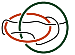
(a)

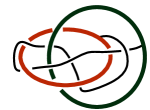
(b)

Figure 4.6. $\mp A_{2}$-twisted $\operatorname{HK}5_{1}$ (Example 4.1).

Example 4.2 ($\operatorname{HK}6_{2}$).

For our second set of examples, we consider the handlebody knot $\operatorname{HK}6_{2}$ corresponding to $\operatorname{6}_{2}$ in Ishii et al.’s knot table [15], and observe that there are two embedded oriented annuli $A_{1}$ and $A_{2}$ in $\mathbb{S}^{3}$ with their interior intersecting with $\operatorname{HK}6_{2}$ at disk $D_{1}$ and $D_{2}$, respectively (see Fig. 4.8; there is an obvious choice for the inner circle for $A_{1}$, whereas for $A_{2}$, we identify the horizontal one as the inner circle of a standard annulus).

Figure 4.7. The handlebody knot $\operatorname{HK}{6}_{2}$.

(a)

(b)

Figure 4.8. Annuli $A_{1}$ and $A_{2}$.

Applying the twist construction to the annuli $A_{1}$ and $A_{2}$, we get two families of handlebody knots with homeomorphic complements. We record $\mp A_{1}$-twisted $\operatorname{HK}6_{2}$ and $\mp A_{2}$-twisted $\operatorname{HK}6_{2}$ in Fig. 4.9 and 4.10

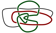
(a)

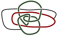
(b)

Figure 4.9. left: $-A_{1}$-twisted $\operatorname{HK}6_{2}$; right: $+A_{1}$-twisted $\operatorname{HK}6_{2}$.

and get the corresponding $-A_{2}$-twisted $\operatorname{HK}6_{2}$ (Fig. 4.10, left) and $+A_{2}$-twisted $\operatorname{HK}6_{2}$ (Fig. 4.10, right).

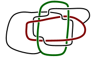
(a)

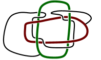
(b)

Figure 4.10. left: $-A_{2}$-twisted $\operatorname{HK}6_{2}$; right: $+A_{2}$-twisted $\operatorname{HK}6_{2}$.

In Subsection 5.4.1 (Tables 1, 2), we shall prove the following results by computing invariants derived from Theorem 3.2.

Proposition 4.1.

The following holds.
$\bullet$ $\operatorname{HK}5_{1}$, $-A_{1}$-twisted $\operatorname{HK}5_{1}$, $+A_{1}$-twisted $\operatorname{HK}5_{1}$ and $+A_{2}$-twisted $\operatorname{HK}5_{1}$ are not ambient isotopic.

$\bullet$ $-A_{2}$-twisted $\operatorname{HK}5_{1}$ is ambient isotopic to $\operatorname{HK}5_{1}$.

$\bullet$ $+A_{1}$-twisted $\operatorname{HK}5_{1}$ has crossing number $=7$.

$\bullet$ Among $\operatorname{HK}6_{2}$, $\mp A_{1}$-twisted $\operatorname{HK}6_{2}$ and $\mp A_{2}$-twisted $\operatorname{HK}6_{2}$, there are at least three inequivalent handlebody knots.

$\bullet$ $-A_{1}$-twisted $\operatorname{HK}6_{2}$ has crossing number $=7$.

4.2. Unswappable scenes

In this short subsection we present a construction of unswappable scenes of genus $3$ and prove Theorem 2.2.

Let $(E,\Sigma,F)$ be a handlebody knot, and suppose there exists a loop $l$ on $\Sigma$ which intersects with only one meridian $m$ in a complete system of meridians of $E$ and bounds a properly embedded disk in $\mathbb{S}^{3}\setminus H_{1}$, where $H_{1}\subset E$ is the solid torus induced by the loop $l$ and the meridian disk bounded by $m$. Then the complement of such a handlebody knot can be expressed as a solid torus with some tunnels in it. For instance, the handlebody knot $\operatorname{HK}5_{1}$ has such a loop:

Figure 4.11. The complement of $\operatorname{HK}5_{1}$ as a solid torus with tunnels in it (middle); the tunnel expression for the complement of $+A_{1}$-twisted $\operatorname{HK}5_{1}$ (right).

the annulus $A_{1}$ in Fig. 4.3 is bounded by $l$, and hence $+A_{1}$-twisted $\operatorname{HK}5_{1}$ can be obtained by twisting the two tubes encircled by $l$; its complement as a solid torus with tunnels is depicted in Fig. 4.11 (right).

Example 4.3 (Unswappable prime scenes of genus $3$).

To construct an unswappable prime scene of genus $3$, we start with a trivial scene of genus $1$ (Fig. 4.12, left). Next, we grow a solid-torus-shaped tree such that the resulting object is the handlebody knot $\operatorname{HK}5_{1}$ (Fig. 4.12, right).

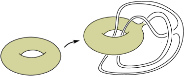
Figure 4.12. $\operatorname{HK}5_{1}$ as a tree on a solid torus.

Then, we dig a tunnel (Fig. 4.13) into the original solid torus in such a way that, without the tree, the resulting object in $\mathbb{S}^{3}$ is the tunnel expression for the complement of $+A_{1}$-$\operatorname{HK}5_{1}$.

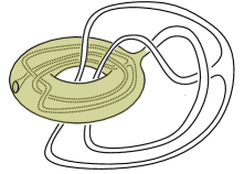
Figure 4.13. Unswappable prime scene of genus $3$.

Denote the resulting connected scene by $\mathcal{S}=(V,\Sigma,W)$. From the construction, it is clear that both $V$ and $W$ are homeomorphic to the connected sum of a solid torus and the complement of $\operatorname{HK}5_{1}$. Hence, it is a symmetric scene.

To see it is not swappable, we note that any diffeomorphism between $V$ and $W$ sends the meridian of $V$ to the meridian of $W$ [34, Corollary $3.6$]. Removing these meridians from $W$ and $V$ in $\mathcal{S}$, one gets a $\operatorname{HK}5_{1}$ and a swapped $+A_{1}$-$\operatorname{HK}5_{1}$, respectively. In particular, if there is an equivalence between $(V,\Sigma,W)$ and $(W,-\Sigma,V)$, then it induces an equivalence between $\operatorname{HK}5_{1}$ and $+A_{1}$-$\operatorname{HK}5_{1}$, which contradicts Proposition 4.1.

Now, suppose $\mathcal{S}$ is not prime and there exists a decomposition $\mathcal{S}=\mathcal{S}_{1}\#\mathcal{S}_{2}$ with $\mathcal{S}_{i}$ a non-trivial scenes of genus $i$, $i=1,2$. Let $\mathbb{S}^{2}\subset\mathbb{S}^{3}$ be the separating $2$-sphere of the decomposition. Then the disk $\mathbb{S}^{2}\cap V$ separates $V$ into a solid torus and the complement of $+A_{1}$-$\operatorname{HK}5_{1}$ and the disk $\mathbb{S}^{2}\cap W$ separates $W$ into a solid torus and the complement of $\operatorname{HK}5_{1}$. So, $\mathcal{S}_{2}=(V_{2},\Sigma_{2},W_{2})$ is such that both $V_{2}$ and $W_{2}$ are $\partial$-irreducible manifolds, which contradicts to Fox’s Theorem [9, p.462 (2)] (see [34, Proposition $2.5$]). Therefore, $\mathcal{S}$ is prime.

This construction works not only for $\operatorname{HK}5_{1}$ but also for other handlebody knots admitting the loop $l$ described at the beginning of the subsection. Combining Motto’s or Lee-Lee’s results with the construction, we see there are infinitely many unswappable prime scenes of genus $3$; this proves Theorem 2.2.

4.3. Bi-knotted scenes

The next examples concern bi-knotted scenes—namely, both “inside” and “outside” are not handlebodies. To construct such examples, we introduce a satellite construction for handlebody knots.

Definition 4.1 (Transverse disks).

Given a handlebody knot $(E,\Sigma,F)$, that is, $E$ being a handlbody, a transverse disk $D$ of $(E,\Sigma,F)$ is a disk in $\mathbb{S}^{3}$ such that $\mathring{D}\cap E$ is the union of $n$ disjoint disks $D_{1},\cdots,D_{n}$ properly embedded in $E$, and $D\setminus\bigcup_{i=1}^{n}\mathring{D}_{i}$ an $n$-times punctured disk properly embedded in $F$.

Definition 4.2 (Neighborhood).

A neighborhood of a transverse disk $D$ of a handlebody knot ${(E,\Sigma,F)}$ is a closed $3$-ball $B$ in $\mathbb{S}^{3}$ containing $D$ in its interior such that $\mathfrak{N}_{1}=B\cap F$ is a tubular neighborhood of $D\setminus\bigcup_{i=1}^{n}\mathring{D}_{i}$ in $F$, and $B\cap E$ is the union of a tubular neighborhood $\mathfrak{N}_{2}$ of $\bigcup_{i=1}^{n}D_{i}$ and a tubular neighborhood $\mathfrak{N}_{3}$ of $\partial D$ in $E$ (see Fig. 4.14).

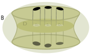
Figure 4.14. A neighborhood $B$ of a transverse disk $D$ with $n=3$.

Construction 4.2 (The satellite construction.).

Identifying $B$ with the unit $3$-ball $B^{3}_{u}\subset\mathbb{R}^{3}$ via a homeomorphism

$$f:(B^{3}_{u},D^{2}_{\mathsf{h}}\times I_{,}\bigcup_{i=1}^{n}D^{2}_{i}\times I)\rightarrow(B,\mathfrak{N}_{1}\cup\mathfrak{N}_{2},\mathfrak{N}_{2}),$$

where $I=[-1,1]$, and $D^{2}_{i}$, $i=1,\cdots,n$, are disjoint disks in the interior of the disk $D_{\mathsf{h}}^{2}$ with radius $\frac{1}{2}$. By convention, we identify $D^{2}_{\mathsf{h}}\times I$ with the subspace

$$C:=\{(x,y,z)\in B^{3}_{u}\mid x^{2}+y^{2}\leq\frac{1}{2}\}\subset B^{3}_{u}$$

via the homeomorphism

$$D^{2}_{\mathsf{h}}\times[-1,1] \rightarrow C$$

$$(x,y,t) \mapsto(x,y,t\sqrt{1-x^{2}-y^{2}}).$$

Now, given an oriented knot $K:\mathbb{S}^{1}\rightarrow\mathbb{S}^{3}$, we choose a basepoint $\ast\in\mathbb{S}^{1}$ and observe that $K$ induces an embedding of arc

$$\mathbb{S}^{1}\setminus\mathfrak{N}(\ast)\xrightarrow{K}\mathbb{S}^{3}\setminus\mathfrak{N}(K(\ast)),$$

where $\mathfrak{N}(\ast)$, $\mathfrak{N}(K(\ast))$ are open tubular neighborhoods of $\ast$ and $K(\ast)$ in $\mathbb{S}^{1}$ and $\mathbb{S}^{3}$, respectively. Identify $S^{3}\setminus\mathring{\mathfrak{N}}(K(\ast))$ with $B^{3}_{u}$ via a homeomorphism $h$, and $S^{1}\setminus\mathring{\mathfrak{N}}(\ast)$ with $I$ via a homeomorphism $l$ such that their composition with $K$ induce an embedding of the interval $I$:

$$K_{h,l}:I\hookrightarrow B^{3}_{u}$$

going from the north pole of $B^{3}_{u}$ to the south pole (see Fig. 4.15).

Let $\mathfrak{N}(K_{h,l}(I))$ be a tubular neighborhood of the embedding arc $K_{h,l}(I)$ in $B_{u}^{3}$ such that $\mathfrak{N}(K_{h,l}(I))\cap\partial B^{3}_{u}=D^{2}_{\mathsf{h}}\times\partial I$. Then $K_{h,l}$ extends to an embedding

$$\tilde{K}_{h,l}:D^{2}_{\mathsf{h}}\times I\rightarrow\mathfrak{N}(K_{h,l}(I))\subset B^{3}_{u}$$

with $\tilde{K}_{h,l}|_{D^{2}_{\mathsf{h}}\times\partial I}$ being the inclusion, and for any given $(x,y)\in D^{2}_{\mathsf{h}}$, the arc $\tilde{K}_{h,l}((x,y),t),t\in I$, is parallel to $\tilde{K}_{h,l}((0,0),t):=K_{h,l}(t),t\in I$.

Figure 4.15. A proper arc in a ball.

Consider the filtration given by

$$\bigcup_{i=1}^{n}D_{i}\times I\subset D^{2}_{\mathsf{h}}\times I\xhookrightarrow{\tilde{K}_{h,l}}B^{3}_{u}\xrightarrow{f}B.$$ (4.2)

Then the new scene $\mathcal{S}^{D,K}={(E^{D,K},\Sigma^{D,K},F^{D,K})}$ (Fig. 4.16) obtained by performing the satellite construction along $K$ w.r.t. $D$ on $\mathcal{S}$ is given by

$$\Sigma^{D,K} :=f\circ\tilde{K}_{h,l}\big{(}\partial D_{\mathsf{h}}^{2}\times I\cup_{i}\partial D_{i}^{2}\times I\big{)}\bigcup\overline{\Sigma\setminus B}$$

$$E^{D,K} :=f\Big{(}\overline{B^{3}_{u}\setminus\tilde{K}_{h,l}(D_{\mathsf{h}}^{2}\times I)}\cup_{i}\tilde{K}_{h,l}(D^{2}_{i}\times I)\Big{)}\bigcup\overline{E\setminus B}$$

$$F^{D,K} :=f\circ\tilde{K}_{h,l}\big{(}(D_{\mathsf{h}}^{2}\setminus\cup_{i}D_{i}^{2})\times I\big{)}\bigcup\overline{F\setminus B}.$$

Figure 4.16. The new scene $\mathcal{S}^{D,K}$ (right) obtained by performing the satellite construction along $K$ w.r.t. $D$ on $\mathcal{S}$ (left).

To see that ${(E^{D,K},\Sigma^{D,K},F^{D,K})}$ is independent of all choices involved, we first note that, in view of the tubular neighborhood theorem, it suffices to consider another embedding

$$K^{\prime}:\mathbb{S}^{1}\hookrightarrow\mathbb{S}^{3}$$

that has the same knot type as $K$, and another identifications

$$f^{\prime}:(B^{3}_{u},D^{2}_{\mathsf{h}}\times I_{,}\bigcup_{i=1}^{n}D^{2}_{i}\times I) \rightarrow(B,\mathfrak{N}_{1}\cup\mathfrak{N}_{2},\mathfrak{N}_{2})$$

$$h^{\prime}:B^{3}_{u} \rightarrow\mathbb{S}^{3}\setminus\mathfrak{N}(K^{\prime}(\ast))$$

$$l^{\prime}:I \rightarrow\mathbb{S}^{1}\setminus\mathfrak{N}(\ast).$$

As with $h,l,K$, the homeomorphisms $h^{\prime},l^{\prime},K^{\prime}$ together induce an embedding

$$\tilde{K}^{\prime}_{h^{\prime},l^{\prime}}:D^{2}_{\mathsf{h}}\times I\rightarrow\mathfrak{N}(K_{h,l}(I))\subset B^{3}_{u}$$

with $\tilde{K}^{\prime}_{h^{\prime},l^{\prime}}|_{D^{2}_{\mathsf{h}}\times\partial I}$ being the inclusion, and for any given $(x,y)\in D_{\mathsf{h}}^{2}$, the arc $\tilde{K}^{\prime}_{h^{\prime},l^{\prime}}((x,y),t),t\in I$, is parallel to $\tilde{K}^{\prime}_{h^{\prime},l^{\prime}}((0,0),t):=K^{\prime}_{h^{\prime},l^{\prime}}(t),t\in I$.

Since $K,K^{\prime}$ have the same knot type, there exists $g:B^{3}_{u}\rightarrow B^{3}_{u}$ with

$$g|_{\mathfrak{N}(K_{h,l}(I))\cap\partial B^{3}_{u}}={\operatorname{id}}$$

such that the diagram commutes

(4.3)

In view of (4.3), we may further assume that $g|_{\partial B^{3}_{u}}={\operatorname{id}}$.

Now observe that if there is an isotopy

$$\Phi_{t}:(B^{3}_{u},D^{2}_{\mathsf{h}}\times I_{,}\cup_{i=1}^{n}D^{2}_{i}\times I)\rightarrow(B,\mathfrak{N}_{1}\cup\mathfrak{N}_{2},\mathfrak{N}_{2})$$

between $f,f^{\prime}$, then via the collar of $\partial B\subset\mathbb{S}^{3}$, the scenes obtained by $(f,h,l,K,\mathfrak{N}(K))$ and $(f^{\prime},h^{\prime},l^{\prime},K^{\prime},\mathfrak{N}(K^{\prime}))$ are equivalent. Thus in general, it may be assumed that ${f^{\prime}}^{-1}f$ restricts to the identity on $\partial B^{3}_{u}\setminus(\mathring{D}^{2}_{\mathsf{h}}\times I)\cup\partial D_{\mathsf{h}}^{2}\times I$. Define $F$ to be

$$F(x):=\begin{cases}\tilde{K}_{h,l}{f^{\prime}}^{-1}f\tilde{K}_{h,l}^{-1}(x),&x\in\mathfrak{N}(K_{h,l}(I))\\ g(x),&x\in\overline{B^{3}_{u}\setminus\mathfrak{N}(K_{h,l}(I))}.\end{cases}$$ (4.4)

$F$ is well-defined since $f^{{}^{\prime}-1}f|_{\partial D^{2}_{\mathsf{h}}\times I}={\operatorname{id}}$ and (4.3). Then we have a commutative diagram

(4.5)

Since $f^{{}^{\prime}-1}Ff$ restricts to the identity on $\partial B$, together with the identity map on $\mathbb{S}^{3}\setminus\mathring{B}$, it induces an equivalence between scenes obtained by $(f,h,l,K,\mathfrak{N}(K))$ and $(f^{\prime},h^{\prime},l^{\prime},K^{\prime},\mathfrak{N}(K^{\prime}))$.

We note that by the construction of ${(E^{D,K},\Sigma^{D,K},F^{D,K})}$, there is a natural homeomorphism $\iota:F\rightarrow F^{D,K}$ given by

$$\iota_{|_{F\setminus B}} ={\operatorname{id}}$$

$${\iota_{K}}_{|_{F\cap B}} :F\cap B\xrightarrow{f^{-1}}(D\setminus\bigcup_{i=1}^{n}\mathring{D}_{i})\times I\xrightarrow{f\circ\tilde{K}_{h,l}}F^{D,K}\cap B.$$ (4.6)

On the other hand, the topology of $E^{D,K}$ might change. Whether $\mathcal{S}^{D,K}$ and $\mathcal{S}$ are equivalent depends solely on whether $\partial D\subset E$ is essential.

Lemma 4.3.

Given a handlebody knot $\mathcal{S}=(E,\Sigma,F)$ with a transverse disk $D$, if $\partial D$ bounds a disk in $E$, then $\mathcal{S}^{D,K}$ is equivalent to $\mathcal{S}$, for any knot $K$.

Proof.

Suppose $\partial D$ bounds a proper disk $D^{\prime}$ in $E$. Let $\mathfrak{N}(D^{\prime})$ be a tubular neighborhood of $D^{\prime}$ in $E$. Then the closure complement of $\mathfrak{N}(D^{\prime})$ is a $3$-ball $\tilde{B}\subset\mathbb{S}^{3}$ containing $F$ with $D$ properly embedded in $\tilde{B}$. Take a tubular neighborhood $\mathfrak{N}(D)$ of $D$ in $\tilde{B}$ such that $\mathfrak{N}(D)\cap F$ is a tubular neighborhood of $D\setminus\bigcup_{i=1}^{n}\mathring{D}_{i}$ in $F$, and denote by $B_{1},B_{2}$ components of $\tilde{B}\setminus\mathring{\mathfrak{N}}(D)$. Note that, properly choosing a tubular neighborhood $\mathfrak{N}(\partial D)$ of $\partial D$ in $\mathfrak{N}(D^{\prime})$ gives us a neighborhood $B:=\mathfrak{N}(D)\cup\mathfrak{N}(\partial D)$ of $D$ with which we can perform the satellite construction (4.2) (see Fig. 4.17).

Let $(f,h,l,\mathfrak{N}(K))$ be a choice of homeomorphisms and tubular neighborhood of an oriented knot $K$. Then performing the satellite construction along $K$ w.r.t. $D$ amounts to reembedding $F$ via the composition

$$F\subset\tilde{B}=B_{1}\cup\mathfrak{N}(D)\cup B_{2}\xrightarrow{\mathbf{K}}\mathbb{S}^{3},$$ (4.7)

where $\mathbf{K}$ is the identity on $B_{1}\cup B_{2}$, and is the composition

$$\mathfrak{N}(D)\xrightarrow{f^{-1}}D^{2}_{\mathsf{h}}\times I\xrightarrow{\tilde{K}_{h,l}}B^{3}_{u}\xrightarrow{f}\mathbb{S}^{3}$$

on $\mathfrak{N}(D)$ (Fig. 4.2). Since any two embeddings of the $3$-ball $\tilde{B}$ in $\mathbb{S}^{3}$ are ambient isotopic, $F^{D,K}$ is isotopic to $F$ in $\mathbb{S}^{3}$. ∎

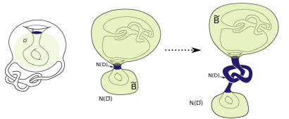
Figure 4.17. Inessential transverse disk.

Fig. 4.17 illustrates the situation in Lemma 4.3. Starting with a solid sphere with an unknotted solid torus removed from the inside, then drilling a cylindrical hole connecting the north pole of the sphere with the northest point of the internal cavity and thus connecting the cavity with the outside, we get a solid set which is topologically equivalent to a solid torus. Attaching some knotted handles to the solids, we further obtain a handlebody knot in $\mathbb{S}^{3}$. Now, take a cross-section of the gallery entering the cave as our transverse disk $D$, whose boundary clearly bounds a disk $D^{\prime}$ in the solid. Then, performing the satellite construction along a knot w.r.t. the disk $D$ is equivalent to substituting the straight gallery by a knotted one. However, it does not change the embedding, since the knotted gallery can be easily untangled by isotoping $D^{\prime}_{0}$, the bottom disk in $\mathfrak{N}(D^{\prime})\simeq D^{\prime}\times I$.

Definition 4.3 (Essential Transverse Disk).

A transverse disk $D$ of a handlebody knot $\mathcal{S}=(E,\Sigma,F)$ is essential if $\partial D$ bounds no disk in $E$.

Lemma 4.4.

Let $D$ be an essential transverse disk of a handlebody knot $\mathcal{S}=(E,\Sigma,F)$ and $K$ a non-trivial oriented knot. Then $\mathcal{S}^{D,K}$ and $\mathcal{S}$ are inequivalent.

Proof.

Let $B$ be a neighborhood of $D$. Then $E\cap\partial B$ is a collection of disks and an annulus $A$. Note that performing the satellite construction along $K$ w.r.t. the disk $D$ does not change the boundary of $B$, but $B\cap E^{D,K}$ is now a union of some tubes and the complement $\mathfrak{C}(K)$ of an open tubular neighborhood of $K$.

Choose a base point $\ast\in A$, and apply van Kampen’s Theorem to the decomposition

$$E^{D,K}=\mathfrak{C}(K)\cup\big{(}E^{D,K}\setminus\mathring{\mathfrak{C}}(K)\big{)}.$$

Then the following pushout diagram computes the fundamental group of $E^{D,K}$.

where the homomorphisms $\iota,\vartheta$ are induced by the inclusions.

The assumption that $\partial D$ does not bound a disk in $E$ implies the homomorphism $\vartheta$ is injective in view of the identification

$$E^{D,K}\setminus\mathring{\mathfrak{C}}(K)\simeq E\setminus\mathring{\mathfrak{N}}(D).$$

On the other hand, $\iota$ sends the generator to the meridian of $K$, and hence is also injective.

The injectivity of $\vartheta$ and $\iota$ implies the other two homomorphisms are injective. In particular, $\pi_{1}(E^{D,K},\ast)$ contains a non-free group $\pi_{1}(\mathfrak{C}(K),\ast)$ since $K$ is non-trivial. In view of the Nielsen–Schreier theorem [31], $E^{D,K}$ cannot be a handlebody and therefore not diffeomorphic to $E$.

∎

From now on, we restrict our attention to handledbody knots of genus $2$.

Definition 4.4 (Type I and II).

Let $\mathcal{S}=(E,\Sigma,F)$ be a handlebody knot of genus $2$. An essential transverse disk $D$ of $\mathcal{S}$ is said to be of type I if $\partial D$ separates $\Sigma$, and of type II otherwise.

Lemma 4.5 (Primeness).

Let $\mathcal{S}=(E,\Sigma,F)$ be a handlebody knot of genus $2$ admitting an essential transverse disk $D$ of type I. Then $\mathcal{S}$ is not prime, and furthermore if $\mathcal{S}=\mathcal{S}_{1}\sharp\mathcal{S}_{2}$ is the prime decomposition of $\mathcal{S}$, then either $\mathcal{S}_{1}$ or $\mathcal{S}_{2}$ is trivial, where $\mathcal{S}_{i}$ is a connected scene of genus one, for $i=1,2$.

Proof.

Observe first that, since $\partial D$ separates $\Sigma$ and does not bound any disks in $E$, given a system of meridian disks of $E$, namely two disjoint disks $M_{1},M_{2}$ such that $E\setminus\mathring{\mathfrak{N}}(M_{1}\cup M_{2})$ is a $3$-ball (compare with [26, p.864], [34, $2.16$]), then $\partial D$ intersects both $\partial M_{1}$ and $\partial M_{2}$.

Now let $\mathring{D}\cap F$ be the union of disjoint disks $D_{1},\cdots,D_{n}$. If $D_{i}$ is essential in $E$, it induces a system of meridian disks of $E$, and hence $\partial D\cap\partial D_{i}\neq\emptyset$, contradicting the fact that $D$ is an embedding in $\mathbb{S}^{3}$. On the other hand, if $D_{i}$ is inessential, we can isotope $D$ away from $D_{i}$ with other components in $E\cap\mathring{D}$ intact. Therefore, it may be assumed that $\mathring{D}\cap F=\emptyset$. Thus $D$ is properly embedded in $F$, and therefore $\mathcal{S}$ is not prime by [34, Prop. $2.15$] and [36, Theorem $1$].

Let $\mathcal{S}=\mathcal{S}_{1}\sharp\mathcal{S}_{2}$ be the prime decomposition of $\mathcal{S}$, and suppose both $\mathcal{S}_{1}$ and $\mathcal{S}_{2}$ are non-trivial. Denote by $F_{1}$ and $F_{2}$ the outsides of $\mathcal{S}_{1},\mathcal{S}_{2}$, respectively—that is, the closures of the complement of the two non-trivial knots, and by $D_{s}$ the intersection of $F$ and a separating sphere $S$ of the decomposition $\mathcal{S}_{1}\sharp\mathcal{S}_{2}$. Then the kernel of the induced homomorphism

$$\pi_{1}(\Sigma,\ast)\rightarrow\pi_{1}(F,\ast)\qquad\ast\in\partial D_{s}\subset\Sigma$$ (4.8)

is the normal closure of the homotopy class $[\partial D_{s}]\in\pi_{1}(\Sigma,\ast)$. Since $D$ is properly embedded in $F$, $[\partial D]$ is also in the kernel of (4.8) and hence is a product of conjugates of $[\partial D_{s}]$.

On the other hand, $[\partial D_{s}]$ is also in the kernel of

$$\pi_{1}(\Sigma,\ast)\rightarrow\pi_{1}(E,\ast),$$ (4.9)

and hence $[\partial D]$ is in the kernel of (4.9) as well; this, however, contradicts the essentiality of $D$ as a transverse disk. Thus one of $\mathcal{S}_{1},\mathcal{S}_{2}$ has to be trivial. ∎

The figure below is an essential transverse disk of type I in a trivial scene. Performing the satellite construction along a trefoil knot w.r.t. the disk produces the complement of the handlebody knot $\operatorname{HK}5_{4}$ ($5_{4}$ in Ishii et al.’s handlebody knot table).

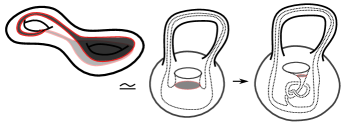
Figure 4.18. Essential transverse disk of type I.

Lemma 4.6 (Meridian with respect to a transverse disk).

Given a prime handlebody knot $\mathcal{S}=(E,\Sigma,F)$ of genus $2$ with an essential transverse disk $D$. Then there exists a system of meridian disks $\{M_{1},M_{2}\}$ of $E$ such that $\partial D$ intersects $M_{1}$ at a single point and $M_{2}\cap\partial D=\emptyset$. Furthermore, if $\{M_{1}^{\prime},M_{2}^{\prime}\}$ is another system of meridian disks with $M_{1}^{\prime}\cap\partial D$ a single point and $M_{2}^{\prime}\cap D=\emptyset$, then $M_{2},M_{2}^{\prime}$ are isotopic in $E$.

Proof.

Since $(E,\Sigma,F)$ is prime, $\mathring{D}\cap E\neq\emptyset$. If one of the disks, say $D_{1}$ in $\mathring{D}\cap E=\bigcup_{i=1}^{n}D_{i}$ is a meridian disk, then we define $M_{2}$ to be $D_{1}$. The complement $\tilde{E}$ of an open tubular neighborhood of $\bigcup_{i=1}^{n}D_{i}$ in $E$ contains exactly one component homeomorphic to a solid torus with $\partial D$ on the boundary of the solid torus since $\partial D$ does not bound any disk in $E$. In particular, the solid torus is unknotted in $\mathbb{S}^{3}$. We define $M_{1}$ to be a meridian disk of the solid torus.

On the other hand, if none of $D_{i}^{\prime}s$ is a meridian disk of $E$, namely $D_{i}^{\prime}s$ all separating $E$, then

$$\tilde{E}:=E\setminus\mathring{\mathfrak{N}}(\bigcup_{i=1}^{n}D_{i})$$

contains two solid tori. One of them contains $\partial D$, while the other does not intersect $D$. We define $M_{1}$ to be the meridian disk of the former, and $M_{2}$ the meridian disk of the latter.

Suppose there is another system of meridian disks $\{M_{1}^{\prime},M_{2}^{\prime}\}$ satisfying $M_{1}^{\prime}\cap D$ is a point and $M_{2}^{\prime}\cap D=\emptyset$. Then we attach a $2$-handle $h^{2}$ to $E$ along a tubular neighborhood of $\partial D$ in $\partial E$. The resulting manifold $\hat{E}:=E\cup h^{2}$ is a solid torus with both $M_{2},M_{2}^{\prime}$ meridian disks of $\hat{E}$.

If $\partial M_{2}\cap\partial M_{2}^{\prime}\neq\emptyset$, then there are at least two arcs of $\partial M_{2}\cap\partial M_{2}^{\prime}$ innermost in $M_{2}$, at least one of which cuts off disks $Q,Q^{\prime}$ from $M_{2},M_{2}^{\prime}$, respectively, such that $Q^{\prime}\cap M_{2}=M_{2}^{\prime}\cap M_{2}$, $D^{\prime\prime}:=Q\cup Q^{\prime}$ inessential in $\hat{E}$, and the $3$-ball component of $\hat{E}\setminus\mathring{\mathfrak{N}}(D^{\prime\prime})$ not containing $h^{2}$. Therefore, it may be assumed that $M_{2},M_{2}^{\prime}$ are disjoint, and the $3$-ball component in $\hat{E}\setminus\mathfrak{N}(M_{2}\cup M_{2}^{\prime})$ not containing $h^{2}$ gives an isotopy between $M_{2}$ and $M_{2}^{\prime}$ in $E$. ∎

Definition 4.5 (Associated meridian).

We call the boundary $m$ of $M_{2}$ in Lemma 4.6 the associated meridian w.r.t. the essential transverse disk $D$.

Given an essential transverse disk $D$ of a prime handlebody knot $(E,\Sigma,F)$, we can identify $E$ with the complement of a trivial scene of genus $2$, $H_{2}\subset\mathbb{S}^{3}$, and $\partial D$ with one of its meridians.

(a)

(b)

Figure 4.19. Realizing E as the complement of a trivial scene.

Then $E^{D,K}$ is homeomorphic to the outside of the scene obtained by performing the satellite construction along $K$ w.r.t. a transverse disk bounded by $\partial D$ in $H_{2}$.

Lemma 4.7 (Meridians into meridians).

Let $\mathcal{S}=(E,\Sigma,F)$, $\mathcal{S}^{\prime}=(E^{\prime},\Sigma^{\prime},F^{\prime})$ be connected prime handlebody knots of genus two, and $D$, $D^{\prime}$ essential transverse disks in $\mathcal{S}$ and $\mathcal{S}^{\prime}$, and $m$, $m^{\prime}$ the associated meridians w.r.t. $D,D^{\prime}$, respectively. Then any equivalence between $\mathcal{S}^{D,K}$ and $\mathcal{S}^{{}^{\prime}D^{\prime},K}$ can be isotoped such that it sends $m$ to $m^{\prime}$.

Proof.

Observe first that $E^{D,K}\simeq E^{{}^{\prime}D^{\prime},K}$ have the prime decomposition

$$E^{D,K}\simeq V\#\mathfrak{C}(K)\simeq E^{{}^{\prime}D^{\prime},K},$$

where $\mathfrak{C}(K)$ is the complement of an open tubular neighborhood of $K$ (see Fig. 4.19), and $m$ and $m^{\prime}$ can be identified with meridians of the solid torus $V$. By [34, $3.4;3.6$], up to isotopy any diffeomorphism between $E^{D,K}$ and $E^{{}^{\prime}D^{\prime},K}$ sends $m$ to $m^{\prime}$. On the other hand, any equivalence between $\mathcal{S}^{D,K}$ and $\mathcal{S}^{{}^{\prime}D^{\prime},K}$ induces a diffeomorphism between $E^{D,K}$ and $E^{{}^{\prime}D^{\prime},K}$, and hence can be isotoped such that $m$ is sent to $m^{\prime}$. ∎

Example 4.4 (Handcuff).

Consider a handcuff graph $\mathsf{G}$ (left in (4.10)). Attach two $2$-cells (right in (4.10)) to its two circles, respectively.

(4.10)

The resulting space is a $2$-dimensional $CW$-complex $\mathsf{X}$. Let $\iota:\mathsf{X}\rightarrow\mathbb{S}^{3}$ be a map such that its restrictions $\iota|_{\mathsf{G}}$, $\iota|_{\mathsf{D}}$, and $\iota|_{\mathsf{D}^{\prime}}$ are embeddings, and intersections between the two $2$-cells $D:=\iota(\mathsf{D})$ and $D^{\prime}:=\iota(\mathsf{D}^{\prime})$, and between each of them and $G:=\iota(\mathsf{G})$ are transversal.

A tubular neighborhood $E_{G}$ of $G$ induces a handlebody knot

$$\mathcal{S}_{G}=(E_{G},\partial E_{G},F_{G}),$$

where $F_{G}$ is the closure of the complement of $E_{G}$ in $\mathbb{S}^{3}$, and $D,D^{\prime}$ give two transverse disks of $\mathcal{S}_{G}$. It is not always possible to perform the satellite construction w.r.t. $D,D^{\prime}$ at the same time in general as $D\cap D^{\prime}$ might not be empty.

Denote by $\mathcal{S}_{G}^{K}=(E_{G}^{K},\partial E_{G}^{K},F_{G}^{K})$ and $\mathcal{S}_{G}^{\prime,K}=(E_{G}^{\prime,K},\partial E_{G}^{\prime,K},F_{G}^{\prime,K})$ the connected scenes obtained by performing the satellite construction along an oriented knot $K$ w.r.t. $D$ and $D^{\prime}$, respectively. Then the $3$-manifolds $E^{K}_{G}$ and $E^{\prime,K}_{G}$ (resp. $F^{K}_{G}$ and $F^{\prime,K}_{G}$) are homeomorphic, and hence the connected scenes $\mathcal{S}_{G}^{K}$ and $\mathcal{S}_{G}^{\prime,K}$ are bi-knotted scenes with homeomorphic components. Whether or not this pair are equivalent depends on the symmetry of the spatial graph $G\subset\mathbb{S}^{3}$.

For instance, for any of the handcuff diagrams $\operatorname{HK}4_{1}$, $\operatorname{HK}5_{4}$, $\operatorname{HK}6_{5}$, $\operatorname{HK}6_{7}$, $\operatorname{HK}6_{10}$ and $\operatorname{HK}6_{16}$ in [15], there is an obvious isotopy sending the graph to itself with two circles exchanged. Hence, performing the satellite construction w.r.t. $D$ and $D^{\prime}$ results in equivalent scenes. On the other hand, by Theorem 4.7, we have a sufficient condition for $\mathcal{S}_{G}^{K},\mathcal{S}_{G}^{\prime,K}$ to be inequivalent.

Corollary 4.8 (Inequivalence criterion).

Suppose $\mathcal{S}_{G}$ is prime, and $m$ and $m^{\prime}$ be the associated meridians with respect to $D$ and $D^{\prime}$, respectively. If there is no self-homeomorphism of $F_{G}$ sending $m$ to $m^{\prime}$, then $\mathcal{S}_{G}^{K},\mathcal{S}_{G}^{\prime,K}$ are inequivalent, for any non-trivial $K$.

Proof.

Via the homeoomorphism in (4.3), there are identifications

$$F_{G}^{K}\simeq F_{G},\quad F_{G}^{\prime,K}\simeq F_{G};$$

the first homeomorphism preserves $m$, while the second preserves $m^{\prime}$. Thus, by Lemma 4.7, any equivalence between $\mathcal{S}_{G}^{K}$ and $\mathcal{S}_{G}^{\prime,K}$ can be isotoped such that the induced self-homeomorphism of $F_{G}$ sending $m$ to $m^{\prime}$. ∎

Corollary 4.8 and the invariant derived from the fundamental span in Section 5 imply the following:

Theorem 4.9 (Inequivalence of Ishii et al’s handcuffs).

The connected scenes obtained by performing the satellite construction w.r.t. $D$ and $D^{\prime}$ along a non-trivial $K$ on any of the handcuff graph diagrams $\operatorname{HK}5_{1}$, $\operatorname{HK}6_{1}$, and $\operatorname{HK}6_{11}$ in [15] are inequivalent.

In particular, taking one of handcuff graph diagrams in Theorem 4.9, and performing the satellite construction along inequivalent oriented knots w.r.t. $D;D^{\prime}$, we get a an infinite family of pairs of inequivalent connected scenes with homeomorphic components.

The only handcuff diagram in Ishii et al.’s handlebody knot table not mentioned yet is $\operatorname{HK}6_{2}$. There is a less obvious diffeomorphism sending $m$ to $m^{\prime}$. The moves in Fig. 4.20 induces a diffeomorphism swapping two circles in the handcuff graph diagram $\operatorname{HK}6_{2}$ of Ishii’s handlebody knot table.

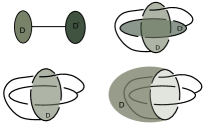
(a)

(b)

Figure 4.20. Symmetry in $\operatorname{HK}6_{2}$.

4.4. Chirality

Chirality of a connected scene concerns the relation between a connected scene and its mirror image; the next definition generalizes the notion of chiral knots.

Definition 4.6 (Mirror image).

Given a connected scene $\mathcal{S}=(E,\Sigma,F)$, its mirror image $m\mathcal{S}=\{mE,m\Sigma,mF\}$ is the connected scene defined as follows: $mE$ is the image of $E$ in $\mathbb{S}^{3}$ under an orientation-reversing self-diffeomorphism of $\mathbb{S}^{3}$, the orientation of $mE$ is induced from $\mathbb{S}^{3}$, $m\Sigma$ is the boundary of $mE$, and $mF:=\overline{\mathbb{S}^{3}\setminus mE}$.

A connected scene $\mathcal{S}$ is chiral if $\mathcal{S}$ and $m\mathcal{S}$ are inequivalent connected scenes; otherwise $\mathcal{S}$ is an amphichiral scene.

In the present paper, we shall restrict our focus on the special case of chiral knots and study the chirality of $9_{42}$ and $10_{71}$ in Rolfsen’s knot table; they are denoted by $\operatorname{K}9_{42}$ and $\operatorname{K}10_{71}$ here to avoid confusion with the notation in Ishii et al.’s handlebody knot table (see Fig. 4.21).

Figure 4.21. $\operatorname{K}9_{42}$ and $\operatorname{K}10_{71}$.

Their chirality cannot be discerned by knot polynomials, such as the Jones polynomial, HOMFLY-PT polynomial and Kauffman polynomial. In the next section, we present a simple invariant, a reinterpretation of Fox’s argument in [10] in terms of the group span with pairing, that can detect their chirality.

5. Invariants of an algebraic scene

In Section 4 we use a generalized Motto-Lee-Lee construction and the satellite construction to produce many inequivalent connected scenes with homeomorphic complements. The aim of the section is to devise tools to investigate these examples. The invariants defined here make crucial use of homomorphisms from $\pi_{1}(F,\ast)$ to a finite group $G$ and various subgroups of $\pi_{1}(F,\ast)$ induced from the fundamental span.

The invariants presented in this section are computable, and the major part of the computation are carried out by the program Appcontour developed by the second author [2], [27]. The result of our computation is recorded in Section 5.4.

Given a connected scene $\mathcal{S}=(E,\Sigma,F)$ and a base point $\ast\in\Sigma$, we consider the set $\operatorname{Hom}(\pi_{1}(F,\ast),G)$ of homomorphisms from $\pi_{1}(F,\ast)$ to a finite group $G$. It is clear that this set is independent of the choice of a base point—namely, given two base points $\ast$ and $\ast^{\prime}$ on $\Sigma$, there is a bijection between $\operatorname{Hom}(\pi_{1}(F,\ast),G)$ and $\operatorname{Hom}(\pi_{1}(F,\ast^{\prime}),G)$. Furthermore, there is a left action of $\operatorname{Aut}(G)$ on $\operatorname{Hom}(\pi_{1}(F,\ast),G)$ given by the composition, where $\operatorname{Aut}(G)$ is the automorphisms group of $G$. For the sake of simplicity, we denote the set of all orbits of $\operatorname{Hom}(\pi_{1}(F,\ast),G)$ under the action of $\operatorname{Aut}(G)$ by

$$\mathcal{H}(F)_{G}.$$

In some situations it is more convenient to consider other subgroups of $\operatorname{Aut(G)}$, for instance the inner automorphisms of $G$; the orbit set of $\operatorname{Hom}(\pi_{1}(F,\ast),G)$ under the action of the subgroup is also an invariant of $\mathcal{S}$.

The cardinality of the orbit set $\mathcal{H}(F)_{G}$ is a strong invariant of connected scenes. For example, Ishii, Kishimoto, Moriuchi and Suzuki [15] show that most of the handlebody knots up to six crossings can be distinguished by the number of conjugacy classes of $\operatorname{SL}(2,\mathbb{Z}/p\mathbb{Z})$- and $\operatorname{SL}(3,\mathbb{Z}/p\mathbb{Z})$-representations of $\pi_{1}(F,\ast)$.

However, since $\mathcal{H}(F)_{G}$ and its variants depend only on the homeomorphism type of $F$, they cannot distinguish the examples in Section 4. A finer invariant taking into account the interrelation between $E$, $\Sigma$, and $F$ is required to examine these examples.

5.1. The G-image of meridians of a handlebody knot

In this subsection we present an invariant of handlebody knots, called the $G$-image of meridians, which is derived from the fundamental span and is useful in distinguishing handlebody knots obtained by the twist construction in Section 4.

Definition 5.1 (Proper homomorphism).

Let $\mathcal{S}=(E,\Sigma,F)$ be a handlebody knot. A surjective homomorphism $\phi:\pi_{1}(F,\ast)\to G$ is proper if the composition

$$\phi\circ{i_{F}}_{*}:\pi_{1}(\Sigma,*)\rightarrow\pi_{1}(F,*)\rightarrow G$$

is not onto. An element $\alpha$ in $\mathcal{H}(F)_{G}$ is called proper if $\alpha$ is represented by a proper homomorphism.

Definition 5.2 ($G$-image of meridians).

Let $\mathcal{S}=(E,\Sigma,F)$ be a handlebody knot. Then the $G$-image of meridians of $\mathcal{S}$ is a set of subgroups of $G$, up to automorphisms of $G$, given by

$$G\operatorname{-im}(\mathcal{S}):=\left\{G_{\alpha}\mid\alpha\in\mathcal{H}(F)_{G}\text{ is proper}\right\}.$$

where $G_{\alpha}$ denotes the image of the kernel of ${i_{E}}_{*}$ under the composition $\phi\circ{i_{F}}_{*}$ under any representative $\phi\in\alpha$.

Remark 5.1.

Note that $G\operatorname{-im}(\mathcal{S})$ is well-defined only up to automorphism of $G$. Also, the $G$-image of meridians of a connected scene is independent of the choice of a base point.

The definition of $G$-image of meridians applies to any connected scene. However, since the kernel of ${i_{E}}_{*}$ is less manageable for a general $E$, in the present paper we restrict our attention to the case where $E$ is a $3$-handlebody. In this case, the kernel of ${i_{E}}_{*}$ is the normal closure of meridians of the handlebody knot.

5.2. An invariant for transverse disks

Denote a connected scene $\mathcal{S}$ equipped with a truly transverse disk $D$ by $(\mathcal{S},D)$. Then, given two such pairs $(\mathcal{S},D)$ and $(\mathcal{S}^{\prime},D^{\prime})$, one might want to know whether the connected scenes $\mathcal{S}^{K}=(E^{D,K},\Sigma^{D,K},F^{D,K})$ and $\mathcal{S}^{\prime,K}=(E^{D^{\prime},K},\Sigma^{D^{\prime},K},F^{D^{\prime},K})$ obtained by performing the satellite construction along a knot $K$ w.r.t. $D$ and $D^{\prime}$, respectively, are equivalent. We define a polynomial invariant for such pairs to investigate the problem.

Definition 5.3 ($G$-index).

Given a prime handlebody knot $\mathcal{S}=(E,\Sigma,F)$ with a truly transverse disk $D$ and a finite group $G$. The $G$-index of $(\mathcal{S},D)$ is the polynomial

$$\operatorname{ind}_{G}[\mathcal{S},D](x)=\sum_{i=1}^{+\infty}n_{i}x^{i},$$

where $n_{i}$ stands for the number of elements in $\mathcal{H}(F)_{G}$ that sends $m$, the associated meridian in $\mathcal{S}$ with respect to $D$, to an element of order $i$ in $G$.

Note that the base point might not be on the associated meridian so, to evaluate the order of the image of the meridian, one needs to connect the meridian with the base point by an arc. But changing the connecting arc does not change the conjugacy class of the image of the meridian in $G$.

By Theorem 4.7, any equivalence between $\mathcal{S}^{K}$ and $\mathcal{S}^{\prime K}$ must send $m$, the associated meridian in $\mathcal{S}$ with respect to $D$, to $m^{\prime}$, the meridian in $\mathcal{S}^{\prime}$ with respect to $D^{\prime}$. Hence, we have the following corollary:

Corollary 5.1.

Given two irreducible handlebody scenes with truly transverse disks $(\mathcal{S},D)$ and $(\mathcal{S}^{\prime},D^{\prime})$, if their $G$-indices are not the same, then the resulting connected scenes $\mathcal{S}^{K}$ and $\mathcal{S}^{\prime,K}$ are not equivalent, for any non-trivial knot $K$.

5.3. An invariant for knot chirality

Any equivalence between two knots $\mathcal{S}=(E,\Sigma,F)$, $\mathcal{S}^{\prime}=(E^{\prime},\Sigma^{\prime},F^{\prime})$ induces an orientation-preserving diffeomorphism from $F$ to $F^{\prime}$, which sends the meridian $[m]$ (resp. the preferred longitude $[l]$) in $\pi_{1}(F,\ast)$ to the meridian $[m^{\prime}]$ (resp. the preferred longitude $[l^{\prime}]$) in $\pi_{1}(F^{\prime},\ast)$. Furthermore, since it is orientation-preserving, it sends a positively oriented pair $([m],[l])$ to a positively oriented pair $([m^{\prime}],[l^{\prime}])$. A meridian–longitude pair $([m],[l])$ is positively oriented if its intersection number $d([m],[l])$ is $+1$.

Fix a positively oriented pair $([m],[l])$ in $\mathcal{S}$ and partition the set $\mathcal{H}(F)_{G}$ according to the order of the image of $[m]$ in $G$:

$$\mathcal{H}(F)_{G}=\mathcal{H}(F)_{1}\cup...\cup\mathcal{H}(F)_{n},$$

where $\mathcal{H}(F)_{i}$ contains those homomorphisms sending $[m]$ to an element of order $i$ in $G$.

Now, consider the product $[m][l]$ in $\pi_{1}(F,\ast)$ and observe that the isomorphism induced by an equivalence between $\mathcal{S}$ and $\mathcal{S}^{\prime}$ sends $[m][l]$ to $[m^{\prime}][l^{\prime}]$. Thus, we can further partition each $\mathcal{H}(F)_{i}$ according to the order of the image of $[m][l]$ in $G$:

$$\mathcal{H}(F)_{i}=\mathcal{H}(F)_{i,1}\cup...\cup\mathcal{H}(F)_{i,n_{i}},$$

where $\mathcal{H}(F)_{i,j}$ contains those homomorphisms in $\mathcal{H}(F)_{i}$ that sends $[m][l]$ to an element of order $j$ in $G$; any equivalence between $\mathcal{S}$ and $\mathcal{S}^{\prime}$ induces a bijection between the sets $\mathcal{H}(F)_{i,j}$ and $\mathcal{H}(F^{\prime})_{i,j}$.

In particular, we have the following:

Lemma 5.2.

The set $\mathcal{H}(F)_{i,j}$ is an invariant of the knot $\mathcal{S}=(E,\Sigma,F)$.

Corollary 5.3.

If a knot $\mathcal{S}$ and its mirror image $m\mathcal{S}$ are ambient isotopic—namely an amphichiral knot, then there is a $1$-$1$ correspondence between the sets $\mathcal{H}(F)_{i,j}$ and $\mathcal{H}(mF)_{i,j}$, for every $i,j$.

5.4. Using the invariants in practice

Here we present the result of our computation of the invariants introduced in Section 5. Required appcontour commands and how they are used to obtain the result are recorded in 5.5.

5.4.1. The G-image of meridians

Let $G=A_{5}$, the alternating group of degree $5$. Table 1 describes the $A_{5}$-image of meridians of twisted ${\operatorname{HK}5_{1}}$’s.

Table 1. The $A_{5}$-image of meridians of twisted ${\operatorname{HK}5_{1}}$’s.

Handlebody knots	The $A_{5}$-image of meridians
${\operatorname{HK}5_{1}}$	{$A_{4}$, $A_{4}$, $A_{4}$, $D_{10}$, $D_{10}$}
$-A_{1}$-${\operatorname{HK}5_{1}}$	{$V_{4}$, $A_{4}$ $A_{4}$, $\mathbb{Z}/5\mathbb{Z}$, $D_{10}$}
$+A_{1}$-${\operatorname{HK}5_{1}}$	{$A_{4}$, $A_{4}$, $A_{4}$, $\mathbb{Z}/5\mathbb{Z}$, $D_{10}$}
$-A_{2}$-${\operatorname{HK}5_{1}}$	{$A_{4}$, $A_{4}$, $A_{4}$, $D_{10}$, $D_{10}$}
$+A_{2}$-${\operatorname{HK}5_{1}}$	{$V_{4}$, $A_{4}$, $A_{4}$, $D_{10}$, $D_{10}$}

It appears that the $A_{5}$-image of meridians cannot distinguish $-A_{2}$-${\operatorname{HK}5_{1}}$ and ${\operatorname{HK}5_{1}}$, but in fact, these two handlebody knots are ambient isotopic as shown in Fig: 5.1. Contrary to the families of handlebody knots in [25] and [18], the family of handlebody knots constructed by twisting ${\operatorname{HK}5_{1}}$ along $A_{2}$ contains both equivalent and inequivalent handlebody knots.

Figure 5.1. Equivalence between $-A_{2}$-${\operatorname{HK}5_{1}}$ and ${\operatorname{HK}5_{1}}$.

Table 2 presents the $A_{5}$-image of meridians of twisted ${\operatorname{HK}6_{2}}$’s.

Table 2. The $A_{5}$-image of meridians of twisted ${\operatorname{HK}6_{2}}$’s.

Handlebody knots	The $A_{5}$-image of meridians
${\operatorname{HK}6_{2}}$	{$D_{10}$, $D_{10}$, $D_{10}$, $V_{4}$}
$+A_{1}$-${\operatorname{HK}6_{2}}$	{$A_{4}$, $D_{10}$, $D_{10}$, $D_{10}$}
$-A_{1}$-${\operatorname{HK}6_{2}}$	{$A_{4}$, $D_{10}$, $D_{10}$, $D_{10}$}
$+A_{2}$-${\operatorname{HK}6_{2}}$	{$A_{4}$, $D_{10}$, $D_{10}$, $\mathbb{Z}/5\mathbb{Z}$}
$-A_{2}$-${\operatorname{HK}6_{2}}$	{$A_{4}$, $D_{10}$, $D_{10}$, $\mathbb{Z}/5\mathbb{Z}$}

Among these handlebody knots $+A_{1}$-${\operatorname{HK}5_{1}}$ and $-A_{1}$-${\operatorname{HK}6_{2}}$ have crossing number $7$ because no other handlebody knot in Ishii et al.’s handlebody knot table, except for $-A_{1}$-${\operatorname{HK}5_{1}}$, which is ${\operatorname{HK}6_{4}}$, has its complement homeomorphic to the complement of ${\operatorname{HK}5_{1}}$; similarly, except for ${\operatorname{HK}6_{2}}$, no handlebody knots in the handlebody knot table has its complement homeomorphic to the complement of $-A_{1}$-${\operatorname{HK}6_{2}}$. Therefore, we have proved Proposition 4.1.

5.4.2. The G-index of essential transverse disks

Handlebody knot,	The $S_{4}$-index	The $A_{5}$-index
transverse disk
(${\operatorname{HK}5_{1}}$,$D^{\prime}$)	$5x+20x^{2}+14x^{3}+12x^{4}$	$4x+14x^{2}+21x^{3}+22x^{5}$
(${\operatorname{HK}5_{1}}$,$D$)	$5x+22x^{2}+10x^{3}+14x^{4}$	$4x+15x^{2}+16x^{3}+26x^{5}$
(${\operatorname{HK}6_{1}}$,$D^{\prime}$)	$5x+20x^{2}+14x^{3}+12x^{4}$	$4x+24x^{2}+22x^{3}+27x^{5}$
(${\operatorname{HK}6_{1}}$,$D$)	$5x+18x^{2}+18x^{3}+10x^{4}$	$4x+15x^{2}+28x^{3}+30x^{5}$
(${\operatorname{HK}6_{11}}$,$D^{\prime}$)	$5x+18x^{2}+10x^{3}+10x^{4}$	$4x+11x^{2}+11x^{3}+16x^{5}$
(${\operatorname{HK}6_{11}}$,$D$)	$5x+18x^{2}+10x^{3}+10x^{4}$	$4x+19x^{2}+13x^{3}+6x^{5}$

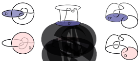
Figure 5.2. $D$ and $D^{\prime}$ in ${\operatorname{HK}5_{1}}$, ${\operatorname{HK}6_{1}}$, and ${\operatorname{HK}6_{11}}$.

From the table above we can see that for the handlebody knot diagrams ${\operatorname{HK}5_{1}}$ and ${\operatorname{HK}6_{1}}$, the $S_{4}$-index can already distinguish the bi-knotted scenes obtained by performing the satellite construction w.r.t. $D$ and $D^{\prime}$, but for ${\operatorname{HK}6_{11}}$, we need the $A_{5}$-index to see that performing the satellite construction w.r.t. $D$ and $D^{\prime}$ induce different bi-knotted scenes. Note that the $A_{4}$-index can distinguish none of them.

5.4.3. Knot chirality

To illustrate how one can use Corollary 5.3 to detect knot chirality, we consider the right-hand trefoil $K$ and its mirror image $mK$:

They have isomorphic fundamental groups:

$$\pi_{1}(K) =<x_{1},x_{2}\hskip 10.00002pt\mid\hskip 10.00002ptx_{2}x_{1}x_{2}=x_{1}x_{2}x_{1}>;$$

$$\pi_{1}(mK) =<y_{1},y_{2}\hskip 10.00002pt\mid\hskip 10.00002pty_{2}y_{1}y_{2}=y_{1}y_{2}y_{1}>.$$

Since different base points are connected by an ambient isotopy, without loss of generality, we may assume the base points are on the arc labeled with $x_{1}$ and $y_{1}$, respectively. The corresponding meridian-longitude pairs are $(x_{1},x_{2}x_{1}x_{2}^{-1}x_{1}x_{2}x_{1}^{-3})$ and $(y_{1},y_{2}^{-1}y_{1}^{-1}y_{2}y_{1}^{-1}y_{2}^{-1}y_{1}^{3})$.

Now, up to automorphisms of $A_{5}$, there is only one homomorphism from $\pi_{1}(F,\ast)$ to $A_{5}$ given by

$$x_{1}\hskip 10.00002pt(\text{resp. }y_{1})\mapsto(12345);$$

$$x_{2}\hskip 10.00002pt(\text{resp. }y_{2})\mapsto(13542),$$

where $F$ is the complement of an open tubular neighborhood of $K$ and $\ast\in\partial F$.

In particular, this implies that $\mathcal{H}(F)_{5}$ contains only one element. Computing the image of the product of the meridian and longitude in $A_{5}$ for each of them, we further get

$$x_{1}x_{2}x_{1}x_{2}^{-1}x_{1}x_{2}x_{1}^{-3}\longmapsto(1);$$

$$y_{1}y_{2}^{-1}y_{1}^{-1}y_{2}y_{1}^{-1}y_{2}^{-1}y_{1}^{3}\longmapsto(13524),$$

respectively. Hence the right-hand trefoil has non-trivial $\mathcal{H}(F)_{5,1}$, whereas the left-hand trefoil has non-trivial $\mathcal{H}(F)_{5,5}$, so they are not equivalent.

Remark 5.2.

Fox’s proof of inequivalence of the granny knot $K_{g}=(E_{g},\Sigma_{g},F_{g})$ and the square knot $K_{s}=(E_{s},\Sigma_{s},F_{s})$ [11, p.39] can also be translated in terms of the invariant $\mathcal{H}(F)_{i,j}$. Their inequivalence follows from the fact that $\mathcal{H}(F_{s})_{5,1}$ contains only one element but $\mathcal{H}(F_{g})_{5,1}$ contains two.

In a similar manner, we may compute the orbit set $\mathcal{H}(F)_{A_{5}}$ for ${\operatorname{K}9_{42}}=(E,\Sigma,F)$; by the result of computations in Appcontour, $\mathcal{H}(F)_{A_{5}}$ consists of seven elements, and three of them are in $\mathcal{H}(F)_{3}$: they send $([m],[l])$, the meridian–longitude pair in ${\operatorname{K}9_{42}}$, to $((3,4,5),())$, $((2,3,5),())$, $((1,4,5),(1,4,5))$, respectively. So, $\mathcal{H}(F)_{3,3}$ contains three elements. The third representation corresponds to the representation sending the meridian-longitude pair in $m{\operatorname{K}9_{42}}$ to $((1,4,5),(1,5,4))$, and hence $\mathcal{H}(mF)_{3,3}$ contains only two elements.

In the case of ${\operatorname{K}10_{71}}=(E,\Sigma,F)$, $G=A_{5}$ or $S_{5}$ is not large enough to see its chiraliy, and we need to consider $\mathcal{H}(F)_{A_{6}}$. Computations in Appcontour show there are three elements in $\mathcal{H}(F)_{5}$ and three in $\mathcal{H}(F)_{4}$. These representations induce the following assignments of $([m],[l])$, the meridian–longitude pair of ${\operatorname{K}10_{71}}$:

$$([m],[l]) \longmapsto((23456),())$$

$$\longmapsto((15246),(15246))$$

$$\longmapsto((16425),(16425))$$

$$([m],[l]) \longmapsto((12)(3456),())$$

$$\longmapsto((16)(2345),(16)(2345))$$

$$\longmapsto((1362)(45),(1362)(45))$$

This implies that $\mathcal{H}(F)_{5,5}$ contains three elements and $\mathcal{H}(F)_{4,2}$ two elements, whereas, in $m{\operatorname{K}10_{71}}$, there is only one element in $\mathcal{H}(mF)_{5,5}$ and none in $\mathcal{H}(mF)_{4,2}$.

5.5. Using appcontour

The computer software appcontour [27] is a tool originally developed to deal with “apparent contours”, i.e. drawings that describe smooth solid objects by projecting fold lines onto a plane.

It was recently extended by adding the capability of computing homomorphisms of groups described by group presentation to a finite group as mentioned in the beginning of Section 5.

As an example, we can count the number of representations of handlebody knot ${\operatorname{HK}5_{1}}$ in the alternating group $A_{5}$ with the command

     $ contour --out ks_A5 HK5_1  Result: 61     with the counting done in $A_{5}$ up to conjugacy by a permutation in $S_{5}$.

Unfortunately, the computation of $\pi_{1}(F,\ast)$ performed by appcontour gives a presentation with no information about the correspondance of the generators with actual loops in $F$. For example, for ${\operatorname{HK}5_{1}}$ we get the following presentation of $\pi_{1}(F,\ast)$

     $ contour --out fg HK5_1  Finitely presented group with 3 generators  <a,b,c; abAcaBAbCbcB>     with no information about the loops corresponding to the three generators. Here capital letters are used as a quick way to refer to the inverse of the generators. For this reason we need to carefully construct by hand an analogue of a Wirtinger presentation of our scene. For instance, for ${\operatorname{HK}5_{1}}$, we could use the one shown in Fig. 5.3 (left).

(a)

(b)

Figure 5.3. Wirtinger presentations of ${\operatorname{HK}5_{1}}$ and ${\operatorname{HK}6_{2}}$.

The syntax that can be fed to the software is as follows:

     fpgroup <a,b,c,d,e,f; baCA,faDA,feDAd,acEC,BcFDf; b,FADadaf,A,FACdaf>     where we have the possibility to add a list of selected elements—elements after the second semicolon—that allows us to keep track of specific elements in $\pi_{1}(F,\ast)$. Here selected elements #1 (b) and #2 (FADadaf) ($m_{1}$ and $m_{2}$ below) correspond to the meridians of ${\operatorname{HK}5_{1}}$ induced by the two circles in the handcuff graph diagram (Fig. 5.3, left); selected elements #3 and #4, denoted by $l_{1}$ and $l_{2}$ in the following, are induced by the two circles, which are the other two generators of the fundamental group of $\partial E$ that pair with #1 and #2, respectively.

We create a file named, say, HK5_1.wirtinger containing the description above to be used as input to appcontour and ask for the description of all elements in $\mathcal{H}(F)_{A_{5}}$ with

     $contour ks_A5 HK5_1.wirtinger -v     which results in a long list of all $61$ homomorphisms described by indicating the image of the three generators followed by the corresponding image of the four selected elements.

To get the table 1, we locate the proper homomorphisms in $\mathcal{H}(F)_{A_{5}}$:

     [...]  ====== Homomorphism #10 defined by the permutations:  (3 4 5)  (2 3 4)  (1 3)(2 4)  Selected element #1 -> (2 5 4)  Selected element #2 -> (2 4 3)  Selected element #3 -> (2 3 5)  Selected element #4 -> (2 4)(3 5)  [...]  ====== Homomorphism #12 defined by the permutations:  (3 4 5)  (2 3 5)  (1 2)(3 5)  Selected element #1 -> (2 3 5)  Selected element #2 -> (2 5 3)  Selected element #3 -> (2 4 5)  Selected element #4 -> (2 4 5)  [...]  ====== Homomorphism #28 defined by the permutations:  (2 3)(4 5)  (3 4 5)  (1 5)(3 4)  Selected element #1 -> (2 5)(3 4)  Selected element #2 -> (3 5 4)  Selected element #3 -> (2 4 5)  Selected element #4 -> (2 3 5)  [...]  ====== Homomorphism #32 defined by the permutations:  (2 3)(4 5)  (1 2)(3 4)  (1 4 5 3 2)  Selected element #1 -> (1 5)(2 4)  Selected element #2 -> (1 5)(2 4)  Selected element #3 -> (1 3)(2 5)  Selected element #4 -> (1 3 5 4 2)  [...]  ====== Homomorphism #48 defined by the permutations:  (1 2 3 4 5)  (2 5)(3 4)  (1 2 4 3 5)  Selected element #1 -> (1 5 4 3 2)  Selected element #2 -> (1 3)(4 5)  Selected element #3 -> (1 4)(2 3)  Selected element #4 -> (1 4)(2 3)  [...]     As an example, the first entry in table 1 is the normal closure of the group generated by $m_{1}$ and $m_{2}$ of homomorphism #10 in the group generated by $m_{1}$, $m_{2}$, $l_{1}$, $l_{2}$, which in this case coincide and are isomorphic to $A_{4}$.

To compute the $A_{5}$-image of meridians for each of the twisted ${\operatorname{HK}5_{1}}$s in Fig. 4.4 and 4.6, it suffices to know the image of the meridians in a complete system of meridians under the proper homomorphisms. We may choose the complete system of meridians induced from Fig. 4.4 and 4.6 (regarded as handcuff graph diagrams) and use the twist construction to identify these meridians with elements in the fundamental group of the closure of the complement of ${\operatorname{HK}5_{1}}$ as follows:

$$m_{1}^{-A_{1}} \dashrightarrow m_{1} m_{1}^{-A_{2}} \dashrightarrow m_{1}^{-1}l_{1}^{-1}m_{1}$$

$$m_{2}^{-A_{1}} \dashrightarrow m_{2}l_{2} m_{2}^{-A_{2}} \dashrightarrow m_{2}l_{2}m_{2}$$

$$m_{1}^{+A_{1}} \dashrightarrow m_{1} m_{1}^{+A_{2}} \dashrightarrow l_{1}m_{1}m_{1}$$

$$m_{2}^{+A_{1}} \dashrightarrow m_{2}l_{2}^{-1} m_{2}^{+A_{2}} \dashrightarrow l_{2}^{-1}.$$

This enables us to compute the $A_{5}$-image of meridians for twisted ${\operatorname{HK}5_{1}}$ using proper homomorphisms from the fundamental group of the complement of ${\operatorname{HK}5_{1}}$ to $A_{5}$.

Similarly, running the command

     $ contour ks_A5 HK6_2.wirtinger -v     where file HK6_2.wirtinger contains the Wirtinger presentation of ${\operatorname{HK}6_{2}}$ in Fig. 5.3 (right), we can get proper homomorphisms of the fundamental group of the complement of ${\operatorname{HK}6_{2}}$ to $A_{5}$. Table 2 can then be completed by identifying the meridians in the complete systems of meridians of twisted ${\operatorname{HK}6_{2}}$’s in Fig. 4.9 and 4.10 (viewed as handcuff graph diagrams) with combinations of $m_{1}$, $m_{2}$, $l_{1}$, and $l_{2}$, meridians and two circles in Fig. 5.3 (right), of ${\operatorname{HK}6_{2}}$ using the twist construction:

$$m_{1}^{-A_{1}} \dashrightarrow m_{1} m_{1}^{-A_{2}} \dashrightarrow m_{1}m_{1}m_{1}l_{1}$$

$$m_{2}^{-A_{1}} \dashrightarrow m_{2}l_{2} m_{2}^{-A_{2}} \dashrightarrow m_{2}^{-1}l_{2}^{-1}$$

$$m_{1}^{+A_{1}} \dashrightarrow m_{1} m_{1}^{-A_{2}} \dashrightarrow m_{1}l_{1}^{-1}m_{1}^{-1}m_{1}^{-1}$$

$$m_{2}^{+A_{1}} \dashrightarrow m_{2}l_{2}^{-1} m_{2}^{+A_{2}} \dashrightarrow m_{2}l_{2}m_{2}m_{2}.$$

In fact, for $A_{2}$-twisted ${\operatorname{HK}6_{2}}$ as well as $A_{2}$-twisted ${\operatorname{HK}5_{1}}$, it is easier to represent $m_{i}^{\pm A_{2}}$ in terms of $\tilde{l}_{1}$ and $\tilde{l}_{2}$, the boundary of $A_{2}$, instead of $l_{1}$ and $l_{2}$.

The $S_{4}$-index and the $A_{5}$-index for a transverse disk in a prime handlebody knot can also be computed with the same command

contour ks$\_G$ file-containing-$\{$group presentation; selected elements$\}$

with one of the meridians $m$ corresponding to the associated meridian of the transverse disk in the selected elements. In our case, we could arrange the selected meridians to be the associated meridians of the two transverse disks induced from a handcuff graph diagram. One could add the multiple of $i$ copies of $m$ as an extra relator to get the coefficient of $x^{i}$ directly.

References

- [1] J. W. Alexander, An example of a simply connected surface bounding a region which is not simply connected, Proc. Natl. Acad. Sci. USA 10 (1924), 8–10.
- [2] G. Bellettini, V. Beorchia, M. Paolini, F. Pasquarelli, Shape Reconstruction from Apparent Contours. Theory and Algorithms, Computational Imaging and Vision, Springer-Verlag (2015) pp. iii-333.
- [3] R. Benedetti, R. Frigerio, R. Ghiloni, The topology of Helmholtz domains, Expo. Math. 30 (2012), 319–375
- [4] J. Cerf, Sur les difféomorphismes de la sphère de dimension trois (), Springer-Verlag, Berlin and New York, Lecture Notes in Math. 53 (1968).
- [5] R. J. Daverman, R.B. Sher, Handbook of Geometric Topology North-Holland, Amsterdam (2001).
- [6] M. Dehn, Über unendliche diskontinuierliche Gruppen, Math. Ann. 71 (1911), 116–144.
- [7] B. Farb, D. Margalit, A Primer on Mapping Class Groups, Princeton University Press, (2011).
- [8] S. Friedl, A. N. Miller, M. Powell, Determinants of amphichiral knots, arXiv:1706.07940 [math.GT].
- [9] R. H. Fox, On the imbedding of polyhedra in 3-space, Ann. of Math. 2(49) (1948), 462–470.
- [10] R. H. Fox, Recent development of knot theory at Princeton, Proceedings of the International Congress of Mathematicians 2 (1950), 453–458.
- [11] R. H. Fox, On the complementary domains of a certain pair of inequivalent knots, Indagationes Mathematicae (Proceedings) 55 (1952), 37–40.
- [12] C. Gordon, J. Luecke, Knots are determined by their complements J. Amer. Math. Soc. 2 (1989), 371–415.
- [13] J. Hempel, 3-manifolds, AMS Chelsea Publishing, Providence, RI, (2004).
- [14] T. Homma, On the existence of unknotted polygons on -manifold in , Osaka Math. J. 6 (1954), 129–134.
- [15] A. Ishii, K. Kishimoto, H. Moriuchi, M. Suzuki, A table of genus two handlebody-knots up to six crossings, J. Knot Theory Ramifications 21 (2012).
- [16] T. Kitano, M. Suzuki, On the number of -representations of knot groups J. Knot Theory Ramifications 21 (2012), 1250035.
- [17] A. G. Kurosh, The theory of groups Translated from the Russian and edited by K. A. Hirsch. 2nd English ed. 2 volumes Chelsea Publishing Co., New York (1960) Vol. 1: 272 pp. Vol. 2: 308 pp.
- [18] J. H. Lee, S. Lee, Inequivalent handlebody-knots with homeomorphic complements, Algebr. Geom. Topol. 12 (2012), 1059–-1079.
- [19] B. C. Mazur, On embeddings of spheres, Acta Math. 105 (1961) 1–-17.
- [20] E. E. Moise, Affine structures in -manifolds: II. Positional Properties of 2-Spheres, Ann. of Math. 55 (1952), 172–176
- [21] J. Munkres Obstructions to the smoothing of piecewise-differentiable homeomorphisms, Bull. Amer. Math. Soc. 65 (5) (1959), 332–334.
- [22] E. E. Moise, Geometric Topology in Dimensions and , Springer-Verlag, Grad. Texts in Math. 47, (1977).
- [23] H. Moriuchi, An enumeration of theta-curves with up to seven crossings J. Knot Theory Ramifications 18 (2) (2009) 67–197.
- [24] H. Moriuchi, A table of -curves and handcuff graphs with up to seven crossings Adv. Stud. Pure Math. Noncommutativity and Singularities: Proceedings of French–Japanese symposia held at IHES in 2006, J.-P. Bourguignon, M. Kotani, Y. Maeda and N. Tose, eds. (Tokyo: Mathematical Society of Japan, 2009), 281–290.
- [25] M. Motto, Inequivalent genus two handlebodies in with homeomorphic complements, Topology Appl. 36(3) (1990), 283–290
- [26] M. Ochiai, Heegaard diagrams of 3-manifolds, Trans. Amer. Math. Soc. 328(2) (1991), 863–879.
- [27] M. Paolini, Appcontour. Computer software. Vers. 2.5.3. Apparent contour. (2018) http://appcontour.sourceforge.net/.
- [28] P. Ramadevi, T. R. Govindarajan, R. K. Kaul, Chirality of knots and and Chern-Simons theory, Mod. Phys. Lett. A9 (1994), 3205–3218.
- [29] R. Riley, Homomorphisms of knot groups on finite groups, Math. Comp. 25 (1971), 603–619
- [30] D. Rolfsen, Knots and Links, AMS Chelsea Publishing, vol.364, 2003.
- [31] O. Schreier Die Untergruppen der freien Gruppe, Abh. Math. Semin. Uni. Hamburg 5 (1927), 161–183.
- [32] W. P. Thurston, Three-dimensional Geometry and Topology, Volume 1, Princeton University Press, (1997).
- [33] J. R. Stallings, A topological proof of Grushko’s theorem on free products Math. Z. 90 (1965), 1–8.
- [34] S. Suzuki, On surfaces in 3-sphere: prime decompositions, Hokkaido Math. J. 4 (1975), 179–195.
- [35] Y. Tsukui, On surfaces in 3-space, Yokohama Math. J. 18 (1970), 93–104
- [36] Y. Tsukui, On a prime surface of genus and homeomorphic splitting of -sphere, The Yokohama Math. J. 23 (1975), 63–75
- [37] F. Waldhausen, Heegaard-Zerlegungen der 3-Sphäre, Topology 7 (1968), 195–203.
- [38] F. Waldhausen, On irreducible 3-manifolds which are sufficiently large, Ann. of Math. 87 (1968), 56–88.
- [39] W. Whitten, Knot complements and groups, Topology 26, Issue 1, (1987), 41–44.