Relationship between the Line Width of the Atomic and Molecular ISM in M33

Abstract

We investigate how the spectral properties of atomic (H i) and molecular (H₂) gas, traced by CO(2-1), are related in M33 on $80$ pc scales. We find the H i and CO(2-1) velocity at peak intensity to be highly correlated, consistent with previous studies. By stacking spectra aligned to the velocity of H i peak intensity, we find that the CO line width ($\sigma_{\rm HWHM}=4.6\pm 0.9$ ${\rm km\,s^{-1}}$; $\sigma_{\rm HWHM}$ is the effective Gaussian width) is consistently smaller than the H i line width ($\sigma_{\rm HWHM}=6.6\pm 0.1$ ${\rm km\,s^{-1}}$), with a ratio of ${\sim}0.7$, in agreement with Druard et al. (2014). The ratio of the line widths remains less than unity when the data are smoothed to a coarser spatial resolution. In other nearby galaxies, this line width ratio is close to unity which has been used as evidence for a thick, diffuse molecular disk that is distinct from the thin molecular disk dominated by molecular clouds. The smaller line width ratio found here suggests that M33 has a marginal thick molecular disk. From modelling individual lines-of-sight, we recover a strong correlation between H i and CO line widths when only the H i located closest to the CO component is considered. The median line width ratio of the line-of-sight line widths is $0.56\pm 0.01$. There is substantial scatter in the H i–CO(2-1) line width relation, larger than the uncertainties, that results from regional variations on $<500$ pc scales, and there is no significant trend in the line widths, or their ratios, with galactocentric radius. These regional line width variations may be a useful probe of changes in the local cloud environment or the evolutionary state of molecular clouds.

1 Introduction

Across large samples of nearby galaxies, several studies show a tight correlation between the surface density of molecular (H₂) gas and star formation rate (SFR) surface density (Kennicutt, 1998; Leroy et al., 2008; Bigiel et al., 2008; Kennicutt et al., 2011), and a lack of correlation with the atomic (H i) gas surface density (Bigiel et al., 2008; Schruba et al., 2011). This result shows that star formation is primarily coupled to the molecular gas, rather than the total (H i + H₂) gas component.

A critical, potentially rate-limiting, step in the star formation process is then the formation of molecular gas. Several mechanisms have been proposed that lead to conditions where molecular gas can readily form (Dobbs et al., 2014). These mechanisms for forming the molecular interstellar medium (ISM) are predicted to act over scales ranging from individual molecular clouds to galactic scales. Recent star formation models have sought to predict the atomic-to-molecular gas fraction from the local environment properties (Blitz & Rosolowsky, 2006; Krumholz et al., 2009; Ostriker et al., 2010; Krumholz, 2013; Sternberg et al., 2014; Bialy et al., 2017) and recover observed properties to within a factor of a few (Bolatto et al., 2011; Jameson et al., 2016; Schruba et al., 2018).

To observe signatures of the molecular ISM, we require observations that resolve giant molecular cloud (GMC) scales ($<100$ pc) in both the atomic and molecular gas. Only within the Local Group can current 21-cm telescopes resolve GMC scales, making studies of M33, M31, and the Magellanic Cloud critical for understanding how the molecular ISM forms. In this paper, we use H i and CO(2-1) observations of M33 with a resolution of $80$ pc to study the spectral properties of the atomic and molecular ISM.

Previous high-resolution studies of H i and CO, used as a tracer of H₂, in the Local Group have identified spectral-line properties that are correlated between these tracers. Wong et al. (2009) and Fukui et al. (2009) compared the H i to CO properties in the Large Magellanic Cloud (LMC) on $40$ pc scales. They found that H i and CO spectral properties are correlated, with a close relationship between the velocities at peak intensity and a suggestive correlation between the H i and CO line widths. However, they also found that the H i temperature and column density are poor predictors for the detection of CO, suggesting that a significant amount of H i emission arises from atomic gas not associated with the molecular gas.

On larger scales ($>100$ pc) where individual clouds are unresolved, several studies have found evidence of a large-scale molecular component, possibly unassociated with CO emission from GMCs on small scales. Garcia-Burillo et al. (1992) found CO emission $\sim 1$ kpc from the plane of the disk in the edge-on galaxy NGC 891, providing direct evidence for a “molecular halo.” More recently, Pety et al. (2013) find evidence for a diffuse molecular disk based on interferometric data ($\sim 50$ pc resolution) recovering only $\sim 50\%$ of the flux from single-dish data. They suggest that the remaining emission is filtered out by the interferometer and must be from larger scales. Using a similar comparison between interferometric and single-dish data, Caldú-Primo et al. (2015) and Caldú-Primo & Schruba (2016) identify a wide velocity component in the CO that is only recovered in single-dish data on scales $>500$ pc.

There is also growing evidence for a significant diffuse molecular component in the Milky Way. Dame & Thaddeus (1994) find excess CO emission in the line wings that may be similar to the wide velocity components in nearby galaxies (Caldú-Primo et al., 2015; Caldú-Primo & Schruba, 2016). Roman-Duval et al. (2016) find $25\%$ of the Milky Way molecular gas mass is in diffuse ¹²CO emission that is extended perpendicular to the Galactic plane beyond the ¹²CO emission where denser gas is detected.

Spectral analyses have found connections between the H i with the bright dense and faint diffuse CO components. The different CO components are highlighted through different analyses, with individual lines-of-sight primarily tracing the bright CO emission, while analyses that study an ensemble of spectra through stacking recover the faint CO emission. Comparing these analyses shows that the properties of the bright and faint CO emission differ. Fukui et al. (2009) find CO line widths in the LMC on $40$ pc scales that are $\sim 30\%$ of the H i line widths along the same lines-of-sight. Similar ratios between the CO and H i are found by Wilson et al. (2011) for 12 nearby galaxies on scales from $\sim 200\mbox{--}1200$ pc, though the H i line widths are estimated at a different resolution from the CO. On similar scales ($\sim 200\mbox{--}700$ pc), with matched resolution between the H i and CO, Mogotsi et al. (2016) found that the CO line widths ($\sigma_{\rm CO}=7.3\pm 1.7$ ${\rm km\,s^{-1}}$) are consistently narrower than the H i ($\sigma_{\rm HI}=11.7\pm 2.3$ ${\rm km\,s^{-1}}$) for a number of nearby galaxies. The average ratio of $\sim 0.6$ between the line widths is much larger than the ratio from Fukui et al. (2009) on smaller scales ($\sim 0.3$).

Stacking analyses consistently have broader CO line widths than those from individual spectra. Combes & Becquaert (1997) found comparable H i and CO line widths in two nearby face-on galaxies ($i<12\degree$). They suggested that the H i and CO emission trace a common, well-mixed kinematic component that differs only in the phase of the gas. Using the same data as Mogotsi et al. (2016), Caldu-Primo et al. (2013) also found similar line widths between the H i and CO ($\sigma_{\rm CO}=12.0\pm 3.9$ ${\rm km\,s^{-1}}$ and $\sigma_{\rm HI}=11.9\pm 3.1$ ${\rm km\,s^{-1}}$) for a number of nearby galaxies. Caldu-Primo et al. (2013) concluded that the wide CO component arises from a faint, large-scale molecular component that is too faint to be detected in individual lines-of-sight. However, a stacked spectrum is broadened due to scatter in the line centre (Koch et al., 2018b), particularly when H i velocities are used to align the CO spectra (Schruba et al., 2011; Caldu-Primo et al., 2013). Characterizing methodological sources of line broadening is critical for understanding the spectral properties of the diffuse molecular component.

In M33, there are differing results regarding a diffuse molecular component. Wilson & Scoville (1990) inferred the presence of diffuse molecular gas from interferometric data recovering $\sim 40\%$ of the flux from single-dish observations. Wilson & Walker (1994) supported this conclusion by demonstrating that the high ¹²CO to ¹³CO line ratio does not result from different filling factors between the two lines. Later, Combes et al. (2012) found a non-zero spatial power-spectrum index on kpc scales and suggested that it arises from a large-scale CO component.

Rosolowsky et al. (2003) and Rosolowsky et al. (2007) also found additional CO emission that did not arise from GMCs, similar to Wilson & Scoville (1990). However, Rosolowsky et al. (2003) localized $90\%$ of the diffuse emission to within $100$ pc of a GMC and suggested that this diffuse emission is from a population of small, unresolved molecular clouds that are too faint for their interferometric observations to detect.

These previous results in M33 and other nearby galaxies suggest that detailed studies of molecular clouds and their local environments may need to account for the presence of diffuse CO emission or bright H i emission along the line-of-sight that is unrelated to the molecular cloud. In this paper, we characterize the relationship between the spectral properties of H i and CO in M33 on $80$ pc scales by stacking spectra and modelling individual lines-of-sight. We then critically compare these two different analyses, constraining how methodological line broadening and unrelated H i or CO emission affects the properties of stacked spectra. M33 is an ideal system for this comparison as we can connect studies of H i and CO performed on larger scales ($>100$ pc) to those on small scales ($<50$ pc).

M33’s flocculent morphology also lies between the nearby galaxies in previous studies, with a sample of more massive spiral galaxies in the lower-resolution studies and the irregular morphology of the LMC observed at higher-resolution. The H i in M33 is an ideal tracer of the flocculent spiral structure. The bright H i is aligned in filaments, similar to the “high-brightness network” identified in other galaxies (Braun, 1997).

We compare the atomic and molecular ISM using H i observations obtained with the Karl G. Jansky Very Large Array (VLA) by Koch et al. (2018b, hereafter K18) and the CO(2-1) data from the IRAM 30-m by Druard et al. (2014), as described in §2. The H i data have a beam size of $20$″, corresponding to physical scales of ${\sim}80$ pc at the distance of M33 (840 kpc; Freedman et al., 2001). Our study builds on work by Fukui et al. (2009) and Druard et al. (2014) by utilizing improved 21-cm H i observations and new techniques for identifying spectral relationships. We focus on comparing M33’s H i and CO distributions along the same lines-of-sight, where we explore the difference in velocity where the H i and CO intensity peaks (§3.1), how the line widths of stacked line profiles compare to those measured at lower resolutions (§3.2), and the distribution of H i and CO line widths from fitting individual spectra (§3.3). We then compare the properties from these two analyses and discern where sources of discrepancy arise (§3.4). Our results show that M33 does not have a significant diffuse molecular disk. We discuss this result and compare to previous findings in §4.

2 Observations

2.1 H i VLA & GBT

We utilize the H i observations presented in K18 and provide a short summary of the observations here. Figure 1 shows the H i integrated intensity map. The observations were taken with the VLA using a 13-point mosaic to cover the inner 12 kpc of M33. The data were imaged with CASA 4.4 using natural weighing and deconvolved until the peak residual reached 3.8 mJy beam^-1 ($7.1$ K) per channel, which is about $2.5$ times the noise level in the data. The resulting data cube has a beam size of $20\arcsec\times 18\arcsec$, a spectral resolution of $0.2$ ${\rm km\,s^{-1}}$, and a $1\mbox{-}\sigma$ noise level of $2.8$ K per channel. This spectral resolution is a factor of $\sim 13$ finer than the CO(2-1) data (§2.2), leading to significantly less uncertainty in the velocity at peak intensity in the H i compared to the CO(2-1).

We combine the VLA data with GBT observations by Lockman et al. (2012) to include short-spacing information. We feather the data sets together using the uvcombine package, which implements the same feathering procedure as CASA. Thus the H i data used in this work provide a full account of the H i emission down to ${\sim}80$ pc scales.

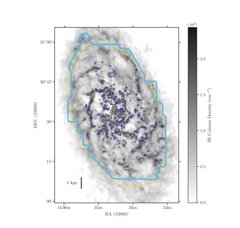
Figure 1: H i and CO(2-1) (contours) column density maps at a resolution of $\sim 80$ pc ($20\arcsec$). The H i column density assumes optically thin emission and is corrected for inclination (K18). The CO(2-1) contour levels (from blue to yellow) indicate surface densities of 900, 1400, 1900, and 2400 ${\rm K\,km\,s^{-1}}$. The light-blue line indicates the extent of the CO(2-1) data, and the dashed yellow line shows the $R_{\rm gal}=7$ kpc galactocentric radius. Qualitatively, the CO(2-1) emission tends to be located with bright H i.

2.2 CO(2-1) IRAM 30-m

We use the CO(2-1) data from the IRAM-30m telescope presented by Druard et al. (2014). Figure 1 shows the region covered by these observations, along with the zeroth moment contours. A full description of the data and reduction process can be found in their §2; a brief summary is provided here. Portions of the map were previously presented by Gardan et al. (2007), Gratier et al. (2010), and Gratier et al. (2012). The data have an angular resolution of $12\arcsec$, corresponding to a physical resolution of ${\sim}48$ pc, and a spectral resolution of $2.6$ ${\rm km\,s^{-1}}$. Because IRAM 30-m is a single dish telescope, the data are sensitive to all spatial scales above the beam size and does not require the feathering step used with the H i (§2.1).

The CO(2-1) cube is a combination of many observations that leads to spatial variations in the noise. The rms noise level differs by a factor of a few in the inner $\sim 7$ kpc of M33’s disk (see Figure 6 in Druard et al., 2014). We adopt the same beam efficiency of $0.56/0.92=0.61$ from Druard et al. (2014) for converting to the main beam temperature. The average noise per channel is $33.3$ mK in units of the main beam temperature. Since we focus only on the line shape properties, we do not require a conversion factor to the H₂ column density in this paper.

The spectral channels are moderately correlated due to the spectral response function of the instrument. Along with broadening due to finite channel widths, the spectral response function correlates nearby channels and broadens the spectra. This broadening can be accounted for by modelling the known spectral response function and accounting for the channel width (Koch et al., 2018a). Adopting the correlation coefficient of $r=0.26$ determined by Sun et al. (2018) for these data, and using the empirical relation from Leroy et al. (2016), we approximate the spectral response function as a three-element Hanning-like kernel with a shape of $[k,\ 1-2k,\ k]$, where $k=0.11$ is the channel coupling. The use of the spectral response function in spectral fitting is described further in §3.3.1.

Throughout this paper, we use a spatially-matched version of these CO(2-1) data convolved to have the same beam size as the H i data . The data are spatially-convolved and reprojected to match the H i data, which lowers the average noise per channel to $16.0$ mK. The spectral dimension is not changed. We create a signal mask for the data by searching for connected regions in the data with a minimum intensity of 2-$\sigma$ that contain a peak of at least 4-$\sigma$. Each region in the mask must be continuous across three channels and have a spatial size larger than the full-width-half-maximum of the beam.

3 H i-CO Spectral Association

We examine the relation between H i and CO(2-1) spectra using three comparisons: (i) the distribution of peak velocity offsets; (ii) the width and line wing excess, and shape parameters of stacked profiles; and (iii) the line widths of both tracers from a limited Gaussian decomposition of the H i associated with CO(2-1) emission. Unless otherwise specified, the line width refers to the Gaussian standard deviation ($\sigma$) and not the full-width-half-maximum (${\rm FWHM}=2\sqrt{2\ {\ln}\ 2}\sigma$).

3.1 Peak Velocity Relation

We first determine the spectral relation between the H i and CO(2-1) by comparing the velocity of the peak temperatures along the same lines-of-sight. We refer to this velocity as the “peak velocity.” Figure 2 compares the absolute peak velocity difference between H i and CO(2-1) versus the peak CO temperature. Most lines-of-sight have peak velocities consistent between the H i and CO(2-1). The standard deviation of the velocity difference, after removing severe outliers with differences of $>10$ ${\rm km\,s^{-1}}$, is $2.7$ ${\rm km\,s^{-1}}$. This is similar to the $2.6$ ${\rm km\,s^{-1}}$ channel width of the CO(2-1) data, suggesting that the peak velocities are typically consistent within the resolution of the CO(2-1) data. Since the peak velocities are defined at the centre of the velocity channel at peak intensity, recovering a scatter in the peak velocity difference of $\sim\pm 1$ channel is reasonable. The much narrower H i channel width ($0.21$ ${\rm km\,s^{-1}}$) accounts for significantly less scatter than the CO(2-1) channel width.

Previous H i-CO studies find a similar correlation between the peak velocities of these tracers and have used the H i to infer the peak velocity of CO(2-1) with the goal of detecting faint CO (Schruba et al., 2011; Caldu-Primo et al., 2013). The brightest CO(2-1) peak intensities tend to have smaller velocity differences between the H i and CO, also consistent with the relation found on $40$ pc scales in the LMC by Wong et al. (2009).

The distribution in Figure 2 has several outliers with velocity differences of $>10$ ${\rm km\,s^{-1}}$, far larger than what would be expected from a Gaussian distribution with a width of $2.7$ ${\rm km\,s^{-1}}$. These outliers account for $3\%$ of the lines of sight and result from locations where the H i spectrum has multiple components and the CO(2-1) peak is not associated with the brightest H i peak (Gratier et al., 2010). In these cases, the CO(2-1) peaks are well-correlated with the peak of the fainter H i component (§3.3). This result is important when stacking spectra (§3.2) aligned with respect to the peak H i temperature. When the CO(2-1) peak is not associated with the brightest H i peak, the CO(2-1) stacked profile will be broadened and could potentially be asymmetric if the CO peaks are preferentially blue- or red-shifted from the H i component. We explore these effects in §3.4.

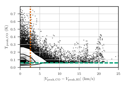
Figure 2: Distribution of the peak CO(2-1) brightness (with ${\rm S/N}>3$) versus the absolute difference in the H i and CO(2-1) peak velocities. The shaded region and contours indicate the regions containing the 1, 2, and 3-$\sigma$ limits of the distribution of points. Individual points show outliers beyond $3\sigma$. The dashed horizontal line is the $3\sigma$ rms noise cut-off in the CO(2-1) data imposed to avoid spurious outliers in the velocity difference. The dotted vertical line is the CO channel width of $2.6$ ${\rm km\,s^{-1}}$. The CO velocities are preferentially located at or near the H i velocities. However, there remains a number of high S/N outliers with a large velocity difference. These outliers occur when the CO emission is associated with a different HI component than the brightest HI peak.

We conclude that the H i peak velocity can nearly always be used to infer the CO(2-1) peak velocity.

3.2 Stacking Analysis

By stacking a large number of spectra aligned to a common velocity, we can examine a high signal-to-noise (S/N) average spectrum of each tracer. Since the signal will add coherently, while the noise will add incoherently, the stacked profiles are ideal for identifying faint emission that is otherwise not detectable in individual lines-of-sight (Schruba et al., 2011). These high S/N spectra can be used to compare the line profile properties of the H i and CO(2-1).

We examine stacked profiles of H i and CO(2-1) aligned with respect to the H i peak velocity since the H i is detected towards nearly every line-of-sight, the H i peak velocity describes the peak CO(2-1) velocity well (§3.1), and the velocity resolution of the H i data is much higher than the CO(2-1) data. We align the spectra by shifting them; we Fourier transform the data, apply a phase shift, and transform back. This procedure preserves the signal shape and noise properties when shifting by a fraction of the channel size. The channel size is a particular issue for the CO(2-1) data, since the channels have a width of $2.6$ ${\rm km\,s^{-1}}$ and the signal in some spectra only spans ${\sim}5$ channels.

Figure 3 shows the stacked profiles, where spectra within a radius of $7$ kpc are included. The H i stacked profile has a kurtosis excess relative to a Gaussian, with enhanced tails and a steep peak. These properties of H i stacked profiles are extensively discussed in K18. The CO(2-1) stacked profile has a qualitatively similar shape but is narrower than the H i profile and has a smaller line wing excess.

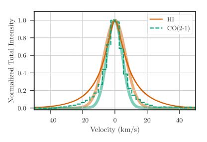
Figure 3: The H i (orange solid) and CO(2-1) (green dashed) stacked profiles shifted with respect to the H i peak velocity. The thick faint lines show the Gaussian model for each tracer. The H i stacked profile is wider and has a larger line wing excess than the CO(2-1) stacked profile.

As in K18, we model the profiles based on the half-width-half-maximum (${\rm HWHM}={\rm FWHM}/2$) approach from Stilp et al. (2013). The model and parameter definitions are fully described in K18; we provide a brief overview here. The HWHM model assumes that the central peak of the profiles can be described by a Gaussian profile whose FWHM matches the profile’s FWHM, which is well-constrained in the limit of high S/N. This model sets the Gaussian standard deviation ($\sigma_{\rm HWHM}={\rm HWHM}/\sqrt{2\,{\rm ln}\,2}$) and central velocity ($v_{\rm peak}$) of this Gaussian, which we refer to as $G(v)$.

The following parameters describe how the observed profile, $S(v)$, compares to the Gaussian model.

The line wing excess expresses the fractional excess relative to the Gaussian outside of the FWHM:

$$f_{\rm wings}=\frac{\sum\limits_{|v|>{\rm HWHM}}\left[S(v)-G(v)\right]}{\sum\limits_{v}S(v)}~{}.$$ (1)

This excess in the line wings can also be used to find the “width” of the wings using a form equivalent to the second moment of a Gaussian:

$$\sigma_{\rm wings}^{2}=\frac{\sum\limits_{|v|>{\rm HWHM}}\left[S(v)-G(v)\right]v^{2}}{\sum\limits_{|v|>{\rm HWHM}}\left[S(v)-G(v)\right]}~{}.$$ (2)

Since the line wing excess will not be close to Gaussian in shape, $\sigma_{\rm wings}$ does not have a clear connection to a Gaussian width.

The asymmetry of a stacked profile is defined as the difference in total flux at velocities greater than and less than $v_{\rm peak}$, normalized by the total flux:

$$a=\frac{\sum\limits_{v>v_{\rm peak}}S(v)-\sum\limits_{v<v_{\rm peak}}S(v)}{\sum S(v)}~{}.$$ (3)

This makes $a$ analogous to the skewness of the profile.

The shape of the peak is described by $\kappa$, defined as the fractional difference between the central peak and the Gaussian model within the FWHM:

$$\kappa=\frac{\sum\limits_{|v|<{\rm HWHM}}\left[S(v)-G(v)\right]}{\sum\limits_{|v|<{\rm HWHM}}G(v)}~{}.$$ (4)

This describes the kurtosis of the profile peak, where $\kappa>0$ is a profile more peaked than a Gaussian and $\kappa<0$ is flatter than a Gaussian. We note that the kurtosis typically describes the line wing structure, however since these regions are excluded in our definition, $\kappa$ describes the shape of the peak.

Since we adopt a semi-parametric model for the stacked profiles, deriving parameter uncertainties also requires a non-parametric approach. We use a bootstrap approach presented in K18 to account for the two significant sources of uncertainty:

1. Uncertainty from the data – These uncertainties come directly from the noise in the data. In each channel, the uncertainty is $\sigma_{\rm RMS}/\sqrt{N_{\rm spec}}$, where $N_{\rm spec}$ is the number of spectra included in the stacked spectrum. We account for this uncertainty by resampling the values in the stacked spectrum by drawing from a normal distribution centered on the original value with a standard deviation equal to the noise. We then calculate the parameters from the resampled stacked spectrum at each iteration in the bootstrap.

2. Uncertainty due to finite channel width – The finite channel width introduces uncertainty in the location of the peak velocity when not explicitly modelled for with an analytic model (Koch et al., 2018a). Since the HWHM model is a semi-parametric model that does not account for finite channel width, we need to adopt an uncertainty for the peak velocity and the inferred line width. We use the HWHM model on very high S/N stacked spectra and assume that the true peak velocity is known to be within the channel of peak intensity. To create an equivalent Gaussian standard deviation for the uncertainty, we scale the rectangular area in the peak channel to the fraction of the area under a Gaussian within $\pm 1\mbox{--}\sigma$, which gives $\sigma_{\rm v_{\rm peak}}=0.34\Delta v$. The HWHM model estimates the width $\sigma_{\rm HWHM}$ based on $v_{\rm peak}$ and thus we adopt the same uncertainty for both parameters. To estimate the uncertainties on the other parameters in the HWHM model, we sample new values of $v_{\rm peak}$ and $\sigma_{\rm HWHM}$ from normal distributions with standard deviations of $0.34\Delta v$ in each bootstrap iteration. These two parameters set the Gaussian shape used to derived the parameters in Equations 1–4.

Based on the bootstrap sampling used in these two steps, we estimate the uncertainties on the remaining HWHM model parameters. Since the stacked profiles have high S/N, the parameter uncertainties are dominated by the uncertainty in $v_{\rm peak}$ and $\sigma_{\rm HWHM}$, and since the CO(2-1) channel size is much larger than the H i ($2.6$ versus $0.2$ ${\rm km\,s^{-1}}$), the CO(2-1) uncertainties are much larger.

Table 1 provides the parameter values and uncertainties from the HWHM model for the stacked profiles in Figure 3. The CO(2-1) line width is $4.6\pm 0.9$ ${\rm km\,s^{-1}}$, which is $70\%$ of the H i width of $6.6\pm 0.1$ ${\rm km\,s^{-1}}$.

Using the same CO(2-1) data at the original $12\arcsec$ resolution, Druard et al. (2014) create CO(2-1) stacked profiles and fit a single Gaussian component to the profile. They find a line width of $\sigma=5.3\pm 0.2$ ${\rm km\,s^{-1}}$, which is $0.7$ ${\rm km\,s^{-1}}$ larger than our measurement using the HWHM method. This discrepancy results from the different modelling approaches used; fitting our CO(2-1) stacked profile with a single Gaussian component gives a line width of $5.4\pm 0.9$ ${\rm km\,s^{-1}}$, consistent with Druard et al. (2014), because the fit is influenced by the line wings.

The profiles are consistent with the same $v_{\rm peak}$, as is expected based on the strong agreement between the peak velocities (§3.1). The scatter in the peak velocity difference will primarily broaden the spectrum, rather than create an offset in $v_{\rm peak}$. We test the importance of this source of broadening in §3.4, but note that the non-Gaussian shape of the stacked profiles makes correcting for this broadening non-trivial. Because of this, we do not apply a correction factor to $\sigma_{\rm HWHM}$ to account for the spectral response function and channel width since the stacked profiles have a non-Gaussian shape.

Table 1: HWHM model parameters for the H i and CO(2-1) stacked profiles for $R_{\rm gal}<7$ kpc at different spatial resolutions. The uncertainties are propagated assuming an uncertainty of half the channel width and the uncertainty of each point in the spectrum is the standard deviation of values within that channel scaled by the square-root of the number of beams.

	H i	CO(2-1)
80 pc (20′′) resolution
$\sigma_{\rm HWHM}$ (${\rm km\,s^{-1}}$)	$6.6\pm 0.1$	$4.6\pm 0.9$
$v_{\rm peak}$ (${\rm km\,s^{-1}}$)	$0.0\pm 0.1$	$-0.2\pm 0.9$
$f_{\rm wings}$	$0.25_{-0.01}^{+0.01}$	$0.21_{-0.10}^{+0.12}$
$\sigma_{\rm wings}$ (${\rm km\,s^{-1}}$)	$24.0_{-0.4}^{+0.3}$	$18_{-3}^{+5}$
$a$	$0.021_{-0.005}^{+0.014}$	$-0.05_{-0.14}^{+0.09}$
$\kappa$	$-0.059_{-0.003}^{+0.004}$	$0.02_{-0.09}^{+0.06}$
160 pc (38′′) resolution
$\sigma_{\rm HWHM}$ (${\rm km\,s^{-1}}$)	$8.0\pm 0.1$	$5.9\pm 0.9$
$v_{\rm peak}$ (${\rm km\,s^{-1}}$)	$-0.1\pm 0.1$	$-0.4\pm 0.9$
$f_{\rm wings}$	$0.19_{-0.01}^{+0.01}$	$0.14_{-0.09}^{+0.10}$
$\sigma_{\rm wings}$ (${\rm km\,s^{-1}}$)	$29.3_{-0.4}^{+0.3}$	$20_{-4}^{+8}$
$a$	$0.012_{-0.012}^{+0.007}$	$-0.07_{-0.10}^{+0.20}$
$\kappa$	$-0.022_{-0.003}^{+0.004}$	$0.00_{-0.06}^{+0.05}$
380 pc (95′′) resolution
$\sigma_{\rm HWHM}$ (${\rm km\,s^{-1}}$)	$8.9\pm 0.1$	$7.2\pm 0.9$
$v_{\rm peak}$ (${\rm km\,s^{-1}}$)	$0.0\pm 0.1$	$-0.2\pm 0.9$
$f_{\rm wings}$	$0.19_{-0.01}^{+0.01}$	$0.15_{-0.07}^{+0.09}$
$\sigma_{\rm wings}$ (${\rm km\,s^{-1}}$)	$32.1_{-0.4}^{+0.3}$	$22_{-3}^{+4}$
$a$	$0.033_{-0.015}^{+0.010}$	$-0.07_{-0.10}^{+0.20}$
$\kappa$	$-0.035_{-0.035}^{+0.004}$	$-0.01_{-0.05}^{+0.05}$

The H i profile is more non-Gaussian in shape than the CO(2-1). The H i profile has a larger line wing excess and a non-Gaussian peak ($\kappa<0$), consistent with the stacked profiles in K18.

The large uncertainties on the CO(2-1) shape parameters make most not significant at the 1-$\sigma$ level, or are consistent within 1-$\sigma$ of the H i shape parameters. Within the uncertainty, the CO(2-1) stacked profiles are symmetric about the peak ($a=0$) and have a Gaussian-shaped profile within the HWHM ($\kappa=0$). The only significant CO(2-1) shape parameter is the line wing excess $f_{\rm wings}$, which is non-zero at the 2-$\sigma$ level and consistent with the H i $f_{\rm wings}$ within 1-$\sigma$. However, there are additional systematics that may contribute to the CO(2-1) $f_{\rm wings}$, including broadening from the distribution of the peak H i and CO velocities (§3.1) and the IRAM 30-m error beam pickup (Druard et al., 2014). We discuss the former contribution in more detail in §3.4. Druard et al. (2014) estimate that the error-beam pickup contributes $2.5\times 10^{6}$ M_⊙, or $1.1\times 10^{4}$ ${\rm K\,km\,s^{-1}}$, using their conversion factor $X_{\rm CO}=4\times 10^{20}$ ${\rm cm}^{-2}/({\rm K\ km\ s}^{-1})$ and a brightness temperature ratio of $0.8$ between the $J=2\mbox{-}1$ and $J=1\mbox{-}0$  CO transitions. The error beam flux may then contribute up to $45\%$ of the $2.4\times 10^{4}$ ${\rm K\,km\,s^{-1}}$ line wing excess. We further assess whether the error beam flux contributes to the line wings in §3.2.1.

Assuming that the error beam does contribute $45\%$ of the CO line wing excess, M33 appears to exhibit weaker line wings compared to those measured in M31 by Caldú-Primo & Schruba (2016). They characterized the CO stacked profiles with a Gaussian model and found that single-dish CO observations in M31 are best fit by two Gaussian components. Their wide Gaussian component would be related to the line wing excess, i.e., a large $f_{\rm wings}$, in our formalism. For the sake of comparison with Caldú-Primo & Schruba (2016), we fit a two-Gaussian component to the CO(2-1) stacked profile and find line widths of $3.8\pm 0.9$ ${\rm km\,s^{-1}}$ and $10.9\pm 0.9$ ${\rm km\,s^{-1}}$ for the narrow and wide Gaussian components, respectively. The narrow line width is similar to the $3.2\pm 0.2$ ${\rm km\,s^{-1}}$ found by Caldú-Primo & Schruba (2016), however their wide component is much narrower, with a width of $6.1\pm 0.6$ ${\rm km\,s^{-1}}$.

3.2.1 Radial Stacked Profiles

We explore trends with galactocentric radius by creating stacked profiles within radial bins of $500$ pc widths out to a maximal radius of $7$ kpc, matching the coverage of the CO(2-1) map. We use a position angle of $201.1\degree$ and inclination angle of $55.1\degree$ for M33’s orientation, based on the H i kinematics from K18. The radial stacking uses the same procedure for the H i profiles as in K18, but with $500$ pc radial bins instead of $100$ pc due to the smaller filling fraction of CO(2-1) detections relative to the H i. The stacked profiles are modeled with the same HWHM model described above.

Figure 4 shows the line widths ($\sigma_{\rm HWHM}$) of the stacked profiles over the galactocentric radial bins (values provided in Table 4). We quantify the relation between galactocentric radius and the line widths by fitting a straight line. We exclude the innermost bins ($<1$ kpc) where beam smearing has a small contribution (Appendix A). To account for the line width uncertainties, we resample the line widths in each bin from a Gaussian distribution with a standard deviation set by the uncertainty (Table 4) in 1000 iterations. We then estimate the slope and its uncertainty using the 15^th, 50^th, and 85^th percentiles from the distribution of 1000 fits. We find that the H i line widths decrease with galactocentric radius ($-0.14\pm 0.01$ ${\rm km\,s^{-1}}$ kpc^-1), consistent with the stacking analysis in 100 pc bins by K18. The decrease in the CO line widths with radius is insignificant at the 1-$\sigma$ level ($-0.16\pm 0.16$ ${\rm km\,s^{-1}}$ kpc^-1). We note, however, that cloud decomposition studies of the CO(2-1) find a shallow line width decrease with galactocentric radius (Gratier et al., 2012; Braine et al., 2018).

Many nearby galaxies have a similar shallow radial decline in the H i and CO line widths, outside of the galaxy centres (Caldu-Primo et al., 2013; Mogotsi et al., 2016). Enhanced line widths are observed in galactic centres that result from a significant increase in the molecular gas surface density or the presence of a bar (e.g., Sun et al., 2018), or due to beam smearing where the gradient of the rotation velocity is significant on the scale of the beam. M33 is a lower mass spiral galaxy and lacks a strong bar, making it likely that the moderate line width increase within $R_{\rm gal}<0.5$ kpc is due to beam smearing (Appendix A).

A clear difference between our results and those by other studies is that the ratio between the CO and H i line width is ${\sim}0.7$, differing from the ratio of $\sim 1.0$ typically measured in other systems on $0.2\mbox{-}0.7$ kpc (Combes & Becquaert, 1997; Caldu-Primo et al., 2013). Since the observation of comparable CO and H i line widths is used as an indicator of a thick molecular gas disk, we discuss this topic in detail in §4.

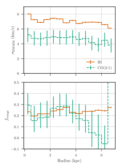
Figure 4: Stacked profile line widths ($\sigma_{\rm HWHM}$; top) and the fractional line wing excess ($f_{\rm wings}$; bottom) measured in $500$ pc radial bins. The widths are based on the HWHM approach from Stilp et al. (2013), and the errors are from a bootstrap approach described in the text. The widths from both tracers show a shallow radial decline and have a consistent line width ratio of ${\sim}0.7$.

Most of the shape parameters from the HWHM model do not show significant trends with galactocentric radius for the CO(2-1) spectra and are insignificant at the $1\mbox{-}\sigma$ level. The line wing excess ($f_{\rm wings}$) is significant for radial bins within $R_{\rm gal}<5$ kpc. At larger radii, the line wings become less prominent, though the CO detection fraction also sharply decreases at these radii and systematic effects—for example, from baseline fitting—strongly affect the stacked profile shapes beyond the HWHM. This leads to the negative line wing excess at $6<R_{\rm gal}<6.5$ kpc and the large excess in the $6.5<R_{\rm gal}<7$ kpc bin. The stacked profiles in Figure 12 of Druard et al. (2014) also clearly suffer from these effects.

In the previous section, we estimated that error beam pick-up can account for up to $45\%$ of $f_{\rm wings}$ in the stacked profiles for $R_{\rm gal}<7$ kpc. Due to galactic rotation, the error-beam pick up will be asymmetric between the halves of the galaxy. To test for this asymmetry, we also stack spectra in galactocentric radial bins separated into the northern and southern halves. Though with significant uncertainties, the asymmetry of the northern half stacked profiles is consistently more negative than the southern half stacked profiles, which have asymmetries that are either positive or near zero. This discrepancy between the halves shows that error beam pick-up accounts for some of the line wing excess.

The other model parameters are consistent between the northern and southern halves of M33.

3.2.2 Stacked profiles at coarser resolution

We further investigate how stacked profile properties change with spatial resolution by repeating our analysis on data smoothed to a resolution of $160$ pc ($38\arcsec$) and $380$ pc ($95\arcsec$). This allows for a more direct comparison to studies of stacked profiles on larger physical scales (Caldu-Primo et al., 2013). At each resolution, we recompute the H i peak velocities and create stacked H i and CO profiles at that resolution. Table 1 gives the HWHM model parameters for these lower-resolution stacked profiles.

The line widths of both H i and CO(2-1) increase at coarser spatial resolution. Based on stacking over the entire galaxy within $R_{\rm gal}=7$ kpc, we find $\sigma_{\rm HI}=8.0\pm 0.1$ ${\rm km\,s^{-1}}$ and $\sigma_{\rm CO}=5.9\pm 0.9$ ${\rm km\,s^{-1}}$ at a resolution of 160 pc, and $\sigma_{\rm HI}=8.9\pm 0.1$ ${\rm km\,s^{-1}}$ and $\sigma_{\rm CO}=7.2\pm 0.9$ ${\rm km\,s^{-1}}$ at a resolution of 380 pc. The CO(2-1) line widths have a larger relative increase than the H i ones, which results in increased ratios of $\sigma_{\rm CO}/\sigma_{\rm HI}=0.70\pm 0.18$, $0.74\pm 0.15$ and $0.81\pm 0.12$ at scales of 80, 160 and 380 pc data, respectively. However, the large uncertainties on the line width ratios makes this increase insignificant at the 1-$\sigma$ level. Using CO observations with higher spectral resolution will decrease these uncertainties and can determine whether this trend is significant.

There are two sources of line broadening that affect $\sigma_{\rm HWHM}$ as the resolution becomes coarser: (i) the dispersion between the H i and CO(2-1) peak velocities, and (ii) beam smearing. Line broadening from the former source is due to aligning the CO(2-1) spectra by the H i peak velocity. At a resolution of 80 pc, we estimate the standard deviation of the peak velocity difference to be $2.7$ ${\rm km\,s^{-1}}$, as described in §3.1. Using the same procedure at the coarser resolutions, we find 1-$\sigma$ standard deviations of $3.1$ and $3.3$ ${\rm km\,s^{-1}}$ at a resolution of 160 and 380 pc, respectively. The increase in the peak velocity difference moderately increases with resolution, but cannot account for the increase in the line widths at coarser resolution.

To address increased line broadening from beam smearing at coarser resolution, we repeat the line stacking in $500$ pc radial bins at each resolution. Figure 5 shows the stacked line widths ($\sigma_{\rm HWHM}$) at the three spatial resolutions. As the resolution becomes coarser, there is a steeper radial gradient in the line widths of both H i and CO, particularly for $R_{\rm gal}<1$ kpc. This radial trend qualitatively matches our estimate of beam smearing from Appendix A. We determine how much of the line width increase with resolution is due to beam smearing with the area-weighted line broadening estimates calculated in Appendix A. For resolutions of 80 and 160 pc, the broadening from beam smearing is similar, with estimates of $2.0^{+2.1}_{-1.8}$ ${\rm km\,s^{-1}}$ and $1.5^{+1.7}_{-0.8}$ ${\rm km\,s^{-1}}$, respectively. The similar levels of beam smearing at 80 and 160 pc imply that the increase in the line width with resolution is not due to beam smearing.

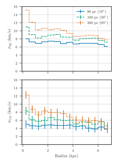
Figure 5: Stacked profile line widths ($\sigma_{\rm HWHM}$) measured in $500$ pc radial bins at three different spatial resolutions for H i (top) and CO(2-1) (bottom). Line widths measured at coarser resolution have a steeper radial gradient due to beam smearing (Appendix A).

At a resolution of 380 pc, beam smearing contributes significantly to the stacked line widths. The area-weighted line broadening from beam smearing is $2.8^{+1.0}_{-1.0}$ ${\rm km\,s^{-1}}$. Treating the stacked profiles as Gaussian within the HWHM, we assume the line broadening can be subtracted in quadrature from the line width. Applying this correction gives line widths of $8.4\pm 0.9$ ${\rm km\,s^{-1}}$ for H i and $6.6\pm 3.6$ ${\rm km\,s^{-1}}$ for CO(2-1). The CO(2-1) line width does not constrain whether the increased line widths are from beam smearing due to the uncertainty from the channel width. However, the $0.9$ ${\rm km\,s^{-1}}$ increase in the H i line width between the 160 and 380 pc data is much larger than the uncertainty and can entirely be explained by beam smearing.

On scales of 380 pc and larger, beam smearing becomes the dominant contribution to the line width. With increasing scale, the stacked H i and CO profiles will approach a common width since the stacking is performed with respect to the H i and will be set by the rotation curve. On smaller scales, systematics in the stacking procedure and beam smearing cannot account for the measured increase in the line widths.

We find that the CO line widths remain smaller than the H i on scales up to $380$ pc, which is within the range where the stacking study by Caldu-Primo et al. (2013) find equivalent CO and H i line widths. We discuss this difference in the ratio of the line widths in M33 to other nearby galaxies in §4.

3.3 H i-CO Line of Sight Comparison

Stacked profiles provide a high S/N spectrum whose properties trace the average of the ensemble of stacked spectra. However, stacking removes information about the spatial variation of individual spectra and distributions of their properties. By fitting individual lines-of-sight, the distributions of line shape parameters that lead to the shape of the stacked spectrum can be recovered.

Describing the H i line profiles with an analytic model is difficult. As we demonstrate in K18, the typical H i line profile in M33 is non-Gaussian due to multiple Gaussian components and asymmetric line wings. The weak relations between the CO and H i integrated intensities found by Wong et al. (2009) in the LMC suggest that much of the H i emission may be unrelated to the CO. With this in mind, and since the CO spectra can typically be modelled with a single Gaussian at this resolution and sensitivity, we use the location of CO emission as a guide to decompose the H i spectra and model the component most likely related to the CO. This is an approximate method; a proper treatment of modeling individual H i spectra requires a robust Gaussian decomposition (Lindner et al., 2015; Henshaw et al., 2016), which is beyond the scope of this paper.

3.3.1 Fitting individual spectra

We relate the H i and CO by using a limited decomposition of the H i based on the spatial and spectral location of CO(2-1) emission. Towards lines-of-sight with CO detections, we determine the parameters of the single Gaussian component that is most closely related to the CO emission.

There are $19{,}796$ spectra where CO(2-1) emission is detected above 3-$\sigma$ in three consecutive channels and is within $R_{\rm gal}<7$ kpc. We model these spectra with the following steps:

1. We fit a single Gaussian to the CO(2-1) spectrum, accounting for broadening due to the channel width and the spectral response function using forward-modelling, which is described in Appendix B. Forward-modelling accounts for line broadening due to the channel width and the spectral response function of the CO(2-1) data (§2.2).

2. The peak velocity of the CO(2-1) fit defines the centre of a search window to find the nearest H i peak. The window is set to a width of three times the FWHM of the CO(2-1) fitted width.

3. Since narrow extragalactic H i spectra have widths $>2$ ${\rm km\,s^{-1}}$ (Warren et al., 2012), we first smooth the H i spectrum with a $2$ ${\rm km\,s^{-1}}$ box-car kernel. Within the search window, we identify the closest H i peak to the CO(2-1) peak velocity.

4. Using the peak temperature of the identified H i peak, we search for the HWHM points around the peak to define the H i fit region.

5. We fit a Gaussian to the un-smoothed H i spectrum within the HWHM points of the identified peak.

This approach assumes that H i spectra are comprised of a small number of Gaussian components with well-defined peaks. Since these restrictions are severely limiting, we define a number of checks to remove spectra that do not satisfy the criteria. A line-of-sight is included in the sample if it meets the following criteria:

1. The H i peak is within the CO(2-1) search window, defined above. Based on visual inspection, H i spectra that contain velocity-blended Gaussian components near the CO(2-1) peak will not satisfy this criterion, and our naive treatment will fail to identify a single H i component.

2. The CO line width is larger than one channel width ($2.6$ ${\rm km\,s^{-1}}$).

3. Ten faint ($T_{\rm HI,peak}<15$ K) H i spectra have a fitted peak associated with noise. The resulting H i fitted profiles have narrow widths ($\sigma<3$ ${\rm km\,s^{-1}}$) and are removed from the sample.

4. The fitted H i peak velocity falls within the HWHM region or its Gaussian width is smaller than $12$ ${\rm km\,s^{-1}}$. This step removes H i spectra with velocity-blended Gaussian components that significantly widen the Gaussian width and are not treated correctly with this method. We set the width threshold based on visual inspection.

5. The CO(2-1) line width is less than $8$ ${\rm km\,s^{-1}}$. A small fraction of CO(2-1) spectra have multiple velocity components, and their fits to a single Gaussian all yield widths larger than $8$ ${\rm km\,s^{-1}}$.

These restrictions yield a clean sample of $15{,}153$ spectra that we analyze here, $76\%$ of the eligible spectra. Table 2 gives the properties of the line width distributions. The uncertainties from each fit are from the covariance matrix of the least-squares fit. We further validate the use of single Gaussian fits in Appendix C and show examples of the fitting procedure.

Table 2: Mean line widths from the line-of-sight spectral fitting at different resolutions. The uncertainties correspond to the 15^th and 85^th percentiles, respectively.

Resolution (pc)	$\sigma$ (${\rm km\,s^{-1}}$)		Fitted $\sigma_{\rm CO}/\sigma_{\rm HI}$
	H i	CO(2-1)
80 (20′′)	$7.4^{+1.7}_{-1.3}$	$4.3^{+1.5}_{-1.0}$	$0.56\pm 0.01$
160 (38′′)	$8.4^{+1.8}_{-1.2}$	$5.0^{+1.4}_{-1.1}$	$0.57\pm 0.01$
380 (95′′)	$11.0^{+2.7}_{-2.0}$	$7.3^{+2.4}_{-1.6}$	$0.63\pm 0.01$

3.3.2 Relations between fitted parameters

We now examine the distributions of fitted H i and CO line parameters to identify which parameters are related.

The fitted peak velocities are strongly correlated (Kendall-Tau correlation coefficient of $0.97$), consistent with the peak velocity over the LOS shown in Figure 2. The agreement is improved, however, since the outliers ($>10$ ${\rm km\,s^{-1}}$) in Figure 2 are removed by only fitting the closest H i component rather than the brightest one. Comparing the fitted peak velocities, the largest velocity difference between the H i and CO is $9.5$ ${\rm km\,s^{-1}}$. The standard deviation between the fitted peak velocities is $2.0$ ${\rm km\,s^{-1}}$, narrower than the $2.7$ ${\rm km\,s^{-1}}$ standard deviation from the line-of-sight peak velocity distribution from §3.1.

We also find that the peak H i temperatures where CO(2-1) is detected increase from $R_{\rm gal}<2$ kpc to $R_{\rm gal}>2$ kpc. The brightest peak H i temperatures ($>80$ K) are primarily found in the spiral arms, or spiral arm fragments, at $R_{\rm gal}>2$ kpc. The lack of spiral structure in the inner $2$ kpc may lead to the lack of peak temperatures over ${\sim}80$ K. These results imply that the H i and CO peak temperatures are not strongly correlated, consistent with the small correlation coefficient of $0.1$ we find using the Kendall-Tau test. The weak correlation in peak temperatures is consistent with Wong et al. (2009), who find that H i peak temperature is poorly correlated to CO detections in the LMC.

The peak CO temperature has a negative correlation with CO line width, as would be expected for a Gaussian profile with a fixed integrated intensity. However, other studies using these CO(2-1) data do not recover this negative correlation. Gratier et al. (2012) find a positive, though weak, correlation between the peak CO temperature and the line width from a cloud decomposition analysis. A similar correlation is found by Sun et al. (2018), who estimate the line widths with the equivalent Gaussian width determined from the peak temperature and integrated intensity of a spectrum (Heyer et al., 2001; Leroy et al., 2016). The discrepancy between our results and these other works is due to requiring three consecutive channels $3\mbox{-}\sigma$ above the rms noise. This biases our LOS sample, leading to incomplete distributions in the peak temperature and integrated intensity.

Figure 6 shows that there is a clear relation between $\sigma_{\rm CO}$ and $\sigma_{\rm HI}$. Though there is significant dispersion in the relation, there is an increasing trend between the line widths of CO(2-1) and H i. We find median line widths of $4.3$ and $7.4$ ${\rm km\,s^{-1}}$ for CO and H i, respectively, on $80$ pc scales. The CO line width distribution is near-Gaussian with a skew to large line widths, with 15^th and 85^th percentiles of $3.3$ and $5.8$ ${\rm km\,s^{-1}}$. The H i distribution is more skewed to larger line widths compared to the CO distribution, and has 15^th and 85^th percentile values of $6.2$ and $9.2$ ${\rm km\,s^{-1}}$. The variations in $\sigma_{\rm HI}$ and $\sigma_{\rm CO}$ are larger than the typical uncertainties of $0.2$ and $0.6$ ${\rm km\,s^{-1}}$, respectively.

We highlight the importance of restricting where the H i is fit to in Appendix C.1, where we show that fitting the whole H i spectrum leads to significant scatter in the H i line widths that severely affects the relationships between the line widths we find here.

Caldú-Primo & Schruba (2016) perform a similar restricted analysis of single Gaussian fitting to CO spectra of M31 at a deprojected resolution of $80\,{\rm pc}\times 380\,{\rm pc}$. From their combined interferometric and single-dish data, they find typical CO line widths of $4.3\pm 1.3$ ${\rm km\,s^{-1}}$, consistent with the range we find.

We characterize the relationship between line widths by fitting for the line width ratio using a Bayesian error-in-variables approach (see Section 8 of Hogg et al., 2010). The goal of this approach is to fully reproduce the data in the model by incorporating (i) the line width uncertainties into the model and (ii) a parameter for additional scatter perpendicular to the line in excess of the uncertainties. We find that $\sigma_{\rm CO}=(0.56\pm 0.01)\ \sigma_{\rm HI}$, which is shown in Figure 6 as the the green dashed line. The scatter parameter in the model is fit to be $0.52\pm 0.02$ ${\rm km\,s^{-1}}$, demonstrating that the scatter in the line width distributions exceeds the uncertainties. This additional scatter represents real variations in the line width distributions.

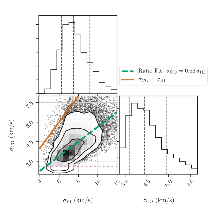
Figure 6: Gaussian widths of individual H i and CO(2-1) profiles. The one-dimensional histograms show the distributions of $\sigma_{\rm HI}$ (top left) and $\sigma_{\rm CO}$ (bottom right) with vertical dashed lines indicating the 15^th, 50^th and 85^th percentiles, respectively. The joint distribution is shown in the bottom left panel. Contours show the area containing data within the 1- to 4-$\sigma$ limits of the distribution and black points show outliers beyond 4-$\sigma$, as described in Figure 2. The orange solid line is the line of equality. The horizontal dotted line indicates the CO(2-1) channel width of $2.6$ ${\rm km\,s^{-1}}$; no samples are included below this width. The green dashed line shows the fitted ratio of $0.56\pm 0.01$. We note that our definition of a ‘clean’ component sample restricts H i line widths to be less than 12 ${\rm km\,s^{-1}}$, and CO line widths must be less than 8 ${\rm km\,s^{-1}}$. Typical uncertainties are $0.6$ and $0.2$ ${\rm km\,s^{-1}}$ for the CO and H i, respectively. A clear relation exists between the H i and CO line widths with intrinsic scatter.

We next examine whether changes in the line width with galactocentric radius can lead to additional scatter in the line width distributions. Similar to the stacking analysis, we fit the line width relation within $500$ pc galactocentric bins out to a radius of $7$ kpc and find no variations in the average widths of the component with galactocentric radius, consistent with the shallow radial decrease from the stacked profile analysis (§3.2). By examining these possible sources of scatter in the line width distributions, we find that none of the sources can fully account for the scatter and that there must be additional variations not accounted for by the relationships of the fitted parameters. We discuss the source of the scatter further in §3.3.4.

3.3.3 The Line Width Ratio at Coarser Spatial Resolution

Similar to the stacked profile analysis (§3.2.2), we repeat the line-of-sight analysis when the data are smoothed to 160 and 380 pc. The same fitting procedure is applied, with similar rejection criteria for poor fits. However, we found that the line widths of valid fits to the data when smoothed to 380 pc can exceed the imposed cut-off values of $12$ and $8$ ${\rm km\,s^{-1}}$ for H i and CO(2-1) due to additional beam smearing on these scales (Appendix A). Based on visual inspection, we increase these cut-off values to $17$ ${\rm km\,s^{-1}}$ and $12$ ${\rm km\,s^{-1}}$.

Table 2 shows the line width distributions at these scales. As we found with the stacked profile widths, the line widths increase at coarser resolution. The line width remains strongly correlated on these scales.

We fit for the line width ratios of the low-resolution samples and find values of $0.57\pm 0.01$ and $0.63\pm 0.01$ for the 160 and 380 pc resolutions, respectively. The fitted ratios indicate that the line width ratio is relatively constant with increasing spatial resolution when analyzed on a line-of-sight basis. We compare these line width ratios to those from the stacking analysis in §3.4.

The line width ratios we find are moderately smaller than the line-of-sight analysis by Mogotsi et al. (2016) for a sample of nearby galaxies. Fitting single Gaussians to H i and CO(2-1) spectra, they find a mean ratio of $0.7\pm 0.2$ on spatial scales ranging from $200\mbox{--}700$ pc. In contrast, the line width ratio we find is significantly steeper than extragalactic studies at higher physical resolution. In the LMC, Fukui et al. (2009) fit Gaussian profiles to both tracers where the CO peaks in a GMC and find a much shallower slope of $0.23$ at a resolution of $40$ pc.

3.3.4 Regional Variations in the H i-CO Line Widths

To further investigate the observed correlation between H i and CO(2-1) line widths and the source of the scatter in this relationship, we highlight the positions of the line widths from three regions in Figure 7. These regions each have peak CO temperatures above the $75^{\rm th}$ percentile, and so the observed scatter is not driven by the correlation between peak CO temperature and line width. By examining many regions on $\sim 100$ pc scales, including the three examples shown, we find that the line widths remain correlated on these scales, but the slope and offset of the line widths varies substantially. These regional variations are the source of the additional scatter required when fitting the H i-CO line width relation (§3.3.2).

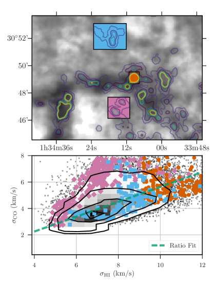
Figure 7: Top: The region around the Northern arm is shown, where the grayscale is the H i column density and contours are the CO(2-1) column densities with same levels shown in Figure 1. The coloured boxes indicate the line widths highlighted below. Bottom: The H i-CO(2-1) line width relation from Figure 6 with line widths highlighted according to their region. The typical uncertainty of the fitted line widths is $0.2$ ${\rm km\,s^{-1}}$ for H i and $0.6$ ${\rm km\,s^{-1}}$ for CO. The H i and CO line widths remain correlated within individual regions, but their position in the line width plane varies with displacements larger than their uncertainties. This suggests the line width relation is sensitive to environmental properties or the evolutionary state of GMCs.

By averaging over these local variations—over the full sample, in radial bins, and at different spatial resolutions—we consistently recover similar line width ratios. The lack of radial variation indicates that $500$ pc radial bins provide a large enough sample to reproduce the scatter measured over the whole disk. If these regional variations arise from individual GMCs, the H i-CO line widths may indicate changes in the local environment or the evolutionary state of the cloud. If the latter is true, the lack of a radial trend is consistent with the radial distribution of cloud evolution types from Corbelli et al. (2017), which are well-mixed in the inner $6$ kpc (see also Gratier et al., 2012).

3.4 Spectral Properties from Stacking versus Individual Lines-of-sight

Previous studies of H i and CO have found differing results between line stacking and fitting individual spectra. While there are some discrepancies in the spectral properties we find, our results from these two methods are more similar than the results from other studies. In this section, we explore the sources of discrepancy between the stacking and line-of-sight fit results and argue that most of the sources are systematic, due to the data or the analysis method.

The stacking analysis and line-of-sight fitting each have relative advantages and disadvantages. Stacked profiles provide an overall census of H i and CO(2-1) without conditioning on the spatial location of the emission. However, variations in the centre and width of individual spectra—along with asymmetries and multiple components—will lead to larger line wings than a Gaussian profile of equivalent width. This result is shown using a mixture model in K18.

The line-of-sight (LOS) analysis retains spatial information, providing distributions of spectral properties that can be connected to different regions. However, the simplistic decomposition of the H i of this analysis requires the detection of CO along the line-of-sight, and so only provides an estimate of H i properties where CO is detected. If H i where CO is detected differs from the global population of H i, the properties we find may not describe the typical H i line properties.

We determine the source of discrepancies in our stacking and fitting results by creating stacked profiles from the fitted LOS sample and their Gaussian models. There are five stacking tests we perform that are designed to control for variations in $\sigma_{\rm HWHM}$ or $f_{\rm wings}$. Table 3 gives the values for these parameters for each of the tests. We described the purpose of each stacking test and their derived line profile properties below:

1. Stacked fitted model components aligned with the fitted CO mean velocity – The fitted Gaussian components, not the actual spectra, are stacked. This removes all emission far from the line centre and will minimize $f_{\rm wings}$ in the stacked profiles. Indeed, $f_{\rm wings}$ for H i and CO(2-1) are both significantly smaller than for the stacked profiles in §3.2 (Table 1). Stacking based on the fitted CO mean velocity will minimize the CO $\sigma_{\rm HWHM}$, while increasing the H i $\sigma_{\rm HWHM}$ due to the scatter between the H i and CO mean velocities. The CO $\sigma_{\rm HWHM}$ is narrower than all of the other stacked profiles, including those from §3.2, and is consistent with the mean CO LOS fitted width of $4.3^{+1.5}_{-1.0}$ ${\rm km\,s^{-1}}$ (Table 2).

2. Stacked fitted model components aligned with the fitted HI mean velocity – This stacking test is identical to (i), except the fitted H i mean velocities are used to align the spectra. Aligning the spectra with the H i mean velocity will decrease the H i $\sigma_{\rm HWHM}$ and increase the CO(2-1) $\sigma_{\rm HWHM}$, consistent with the measured properties.

3. Stacked spectra in the LOS sample aligned with the fitted HI mean velocity – The spectra in the LOS sample, rather than the model components used in (i) and (ii), are stacked aligned with the fitted H i mean velocities. The CO spectra in the sample are required to be well-modelled by a single Gaussian component, but there is a modest increase in $f_{\rm wings}$ to $0.07$., larger than in tests (i) and (ii) The H i spectra, however, have significant line structure that is not modelled for, leading to a vast increase in $f_{\rm wings}$ to $0.19$. The line widths of the H i and CO stacked profiles are the same within uncertainty.

4. Stacked spectra in the LOS sample aligned with the H i peak velocity – The spectra used in (iii) are now aligned with the H i peak velocities from §3.1. These stacked profiles are equivalent to the precedure used in §3.2 using only a sub-set of the spectra. This subset contains some of the outlier points in Figure 2, however $\sigma_{\rm HWHM}$ and $f_{\rm wings}$ do not significantly change from (iii). The outliers in the peak H i and CO velocity difference distribution do not contribute significantly to $\sigma_{\rm HWHM}$ or $f_{\rm wings}$.

5. Stacked spectra in the entire LOS sample, including rejected fits, aligned with the H i peak velocity – Finally, we create stacked profiles for the entire LOS sample considered in §3.3, including the LOS with rejected fits. This test is equivalent to (iv) with a larger sample. Relative to (iv), the H i $\sigma_{\rm HWHM}$ and $f_{\rm wings}$ both moderately increase, as expected when including LOS potentially with multiple bright spectral components. The CO stacked spectrum $\sigma_{\rm HWHM}$ marginally increases compared to (iv), however, $f_{\rm wings}$ increases by $33\%$ to $f_{\rm wings}=0.12$. This increase is driven in part by the CO spectra with multiple components.

Table 3: Stacked line width ($\sigma_{\rm HWHM}$) and line wing excess ($f_{\rm wings}$) from the spectra used in the line-of-sight analysis (§3.3.1). The line widths do not strongly vary when changing the line centre definition or when the Gaussian model components are stacked rather than the actual spectrum. However, $f_{\rm wings}$ is sensitive to whether the full spectra or the models are used. The CO $f_{\rm wings}$ is also more sensitive to the how the stacking is performed than the H i.

	H i	CO(2-1)
(i) Fitted model components aligned to CO Model $v_{0}$
$\sigma_{\rm HWHM}$ (${\rm km\,s^{-1}}$)	$7.6\pm 0.1$	$4.2\pm 0.9$
$f_{\rm wings}$	$0.03_{-0.01}^{+0.01}$	$0.05_{-0.13}^{+0.17}$
(ii) Fitted model components aligned to H i Model $v_{0}$
$\sigma_{\rm HWHM}$ (${\rm km\,s^{-1}}$)	$7.4\pm 0.1$	$4.6\pm 0.9$
$f_{\rm wings}$	$0.03_{-0.01}^{+0.01}$	$0.03_{-0.12}^{+0.16}$
(iii) LOS spectra aligned to H i Model $v_{0}$
$\sigma_{\rm HWHM}$ (${\rm km\,s^{-1}}$)	$7.4\pm 0.1$	$4.8\pm 0.9$
$f_{\rm wings}$	$0.19_{-0.01}^{+0.01}$	$0.07_{-0.12}^{+0.10}$
(iv) LOS Spectra aligned to H i $v_{\rm peak}$
$\sigma_{\rm HWHM}$ (${\rm km\,s^{-1}}$)	$7.3\pm 0.1$	$4.7\pm 0.9$
$f_{\rm wings}$	$0.20_{-0.01}^{+0.01}$	$0.08_{-0.12}^{+0.15}$
(v) All LOS spectra aligned to H i $v_{\rm peak}$
$\sigma_{\rm HWHM}$ (${\rm km\,s^{-1}}$)	$7.6\pm 0.1$	$4.8\pm 0.9$
$f_{\rm wings}$	$0.22_{-0.01}^{+0.01}$	$0.12_{-0.11}^{+0.14}$

From these tests, we can identify the source of the LOS and stacking discrepancies.

3.4.1 Smaller CO LOS fitted line widths than from stacking

The larger CO stacked line widths are due to the scatter between the H i and CO peak velocity (Figure 2). This is demonstrated by comparing tests (i) and (ii), where the former is consistent with the median CO line width from the LOS fitting. The larger CO line width from stacking will lead to an overestimate of the H i-CO line width ratio.

3.4.2 Larger H i LOS fitted line widths compared with stacking

The stacked H i line width towards LOS with CO detections (Table 3) is consistently larger than the H i stacked line width from all LOS (Table 1). There are two possible causes for this discrepancy. First, the H i where CO is detected has larger line widths than the average from all H i spectra. This source requires a physical difference in the atomic gas properties where molecular clouds are located, possibly related to the H i cloud envelope (Fukui et al., 2009). Alternatively, the H i components fitted here may be broadened by overlapping velocity components since our analysis does not account for this. However, from visually examining the fits to the LOS sample, most H i spectra would need to have highly overlapping components for the average H i LOS line width to be broadened, and this does not seem likely for most spectra (Appendix C.2). In order to definitely determine which of these sources leads to the larger H i line widths, we require decomposing the H i spectra without conditioning on the location of the CO emission. However, this analysis is beyond the scope of this paper. We favour larger H i line widths in molecular cloud envelopes as the source of this discrepancy.

3.4.3 Sources of the line wing excess

These five tests provide restrictions on the source of the line wing excess in both tracers. In the H i, $f_{\rm wings}$ is only changed when the model components ((i) and (ii)) are stacked rather than the full H i spectra ((iii)–(v)). This result is consistent with the line structure and wings evident in individual H i spectra, as explored in K18. The scatter in the fitted velocities (H i or CO) can account for $f_{\rm wings}\sim 0.03$ in the stacked H i profiles.

For the CO stacked profiles, there are variations in $f_{\rm wings}$ from multiple sources. There are small contributions to $f_{\rm wings}$ from the scatter in the H i fitted mean velocities (Test (ii); $f_{\rm wings}=0.03$) and the scatter between the H i and CO peak velocities or fitted mean velocities (Tests (iii) & (iv); $f_{\rm wings}=0.01$). Multi-component CO spectra account for $f_{\rm wings}\lesssim 0.04\mbox{--}0.05$ from comparing Tests (iii) and (iv) to Test (v). This estimate is an upper limit since we do not control for contributions from real line wings versus multiple spectral components. Finally, comparing Tests (iii) and (iv) to Test (ii), excess line wings can directly account for $f_{\rm wings}=0.04\mbox{--}0.05$.

The different sources of line wing excess in the CO stacked profiles implies that there is marginal evidence for CO line wings. As described above, stacking systematics and multi-component spectra can account for $f_{\rm wings}\lesssim 0.08\mbox{--}0.09$, roughly half of the line wing excess of $f_{\rm wings}=0.21$ from the stacked profile towards all LOS (Table 1). The discrepancy between the total $f_{\rm wings}$ for the CO stacked profiles and the systematics is then $0.13$, though the large $f_{\rm wings}$ uncertainties can account for the remaining line wing excess. Including the error beam contribution of up to $45\%$ of the line wing excess (§3.2), we find that $\sim 80\%$ of the CO line wing excess can be accounted for without requiring the presence of real CO line wings. However, due to the estimated uncertainties, we cannot rule out their presence.

4 A Marginal Thick Molecular Disk in M33

Studies of CO in the Milky Way and nearby galaxies find evidence of two molecular components: a thin disk dominated by GMCs, and a thicker diffuse molecular disk. Our results, however, suggest that M33 has a marginal thick molecular component, unlike those found in other more massive galaxies, based on (i) finding smaller CO line widths relative to the H i and (ii) the marginal detection of excess CO line wings. In this section, we compare our results to previous studies and address previous works arguing for a diffuse component on large-scales in M33.

Evidence for a diffuse molecular component has been demonstrated with extended emission in edge-on galaxies (e.g., NGC 891; Garcia-Burillo et al., 1992), separating ¹²CO emission associated with denser gas in the Milky Way (Roman-Duval et al., 2016), comparing the flux recovered in interferometric data to the total emission in single-dish observations (Pety et al., 2013; Caldú-Primo et al., 2015; Caldú-Primo & Schruba, 2016), and large CO line widths in nearby galaxies (Combes & Becquaert, 1997; Caldu-Primo et al., 2013; Caldú-Primo et al., 2015).

In M33, a diffuse molecular component has been suggested based on the CO flux recovered in GMCs (Wilson & Scoville, 1990), comparing the ¹³CO to ¹²CO spectral properties (Wilson & Walker, 1994), and a non-zero CO power-spectrum index on kpc scales (Combes et al., 2012). Rosolowsky et al. (2007) find that 90% of the diffuse CO emission is located $<100$ pc to a GMC, and suggest the emission is due to a population of unresolved, low-mass molecular clouds (see also Rosolowsky et al., 2003).

Our stacking analysis, and the stacking analysis in Druard et al. (2014), shows that the CO line widths are consistently smaller than the H i, unlike the line widths from most nearby galaxies on $\sim 500$ pc scales (Combes & Becquaert, 1997; Caldu-Primo et al., 2013). Figure 8 summarizes our results by showing the CO-to-H i line width ratios of the stacked line widths and the radially-binned averages from the line-of-sight analysis at $80$ pc resolution. The ratios from the stacked profiles are consistently $10\%$ larger than the average of the line-of-sight fits due to using the H i peak velocities to align the CO spectra (§3.4). The line width ratio increases but remains less than unity when the data are smoothed to resolutions of $160$ and $380$ pc (§3.2.2), scales comparable to some of the data in Caldu-Primo et al. (2013).

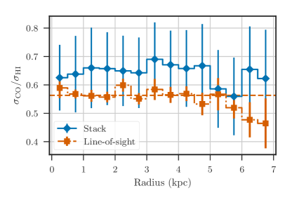
Figure 8: Line width ratio from stacked profiles (blue solid diamonds) and the average from the line-of-sight fits (orange dot-dashed squares) versus galactic radius at $80$ pc ($20\arcsec$) resolution. The 1-$\sigma$ uncertainties on the stacked widths are dominated by the CO(2-1) channel width. The errors on the line-of-sight fits are the standard deviation in the radial bin divided by the square root of the number of independent components. The pink dashed line is the fitted ratio $0.56$ shown in Figure 6. Both methods have line width ratios smaller than unity, unlike other (more massive) nearby galaxies (Caldu-Primo et al., 2013), suggesting M33 lacks a significant thick molecular disk.

Stacking analyses of CO by Caldú-Primo et al. (2015) and Caldú-Primo & Schruba (2016) find a wide Gaussian component to CO stacked profiles that arises only in single-dish observations. The high-resolution ($80\times 350$ pc) CO observations of M31 from Caldú-Primo & Schruba (2016) constrain this wide component to scales of $\sim 500$ pc and larger. Coupled with the large CO line widths, these results suggest the wide Gaussian component is due to a thick molecular disk. In our analysis, the wide Gaussian component would contribute to the line wing excess ($f_{\rm wings}$). In M33, we find a qualitatively similar line wing excess to Caldú-Primo & Schruba, however, up to $\sim 80$% of the excess is due to stacking systematics and error beam pick-up from the IRAM 30-m telescope (§3.4.3; Druard et al., 2014). The remaining fraction of the CO line wing excess is small, and would correspond to a much smaller contribution from a wide Gaussian component compared to those found by Caldú-Primo et al. (2015) and Caldú-Primo & Schruba (2016).

These results strongly suggest M33 has a marginal thick molecular disk and is instead more consistent with the findings from Rosolowsky et al. (2007) where diffuse CO emission is clustered near GMCs and may be due to unresolved low-mass clouds (flux recovery with spatial scale with these CO data is explored in Sun et al., 2018). There remains ambiguity about the diffuse molecular component in M33 from other analyses, and whether M33 is the only nearby galaxy with a marginal thick molecular disk. We address these issues in the following sections. First, we demonstrate that the large-scale CO(2-1) power-spectrum identified in Combes et al. (2012) can be explained by the exponential disk scale of the CO emission rather than a thick molecular disk. We then note the similarity of the line width ratios found by Caldu-Primo et al. (2013) for NGC 2403 and our results.

4.1 Comparison to a thick molecular disk implied by power-spectra

Previous work by Combes et al. (2012) found that the power-spectra of H i and CO integrated intensity maps of M33 have shallow indices extending to kpc scales, with distinct breaks near $\sim 120$ pc where the indices becomes steeper. The non-zero slope on kpc scales suggests there is significant large-scale diffuse emission in M33 from both H i and CO, in contrast with our findings for CO from the line widths.

To explain the non-zero index on large scales, we compare the large-scale distribution of emission in M33 for CO and H i. Bright CO emission is broadly confined to individual regions on scales comparable to the beam size (Figure 1) and has a radial trend in the average surface density that is well-modelled by an exponential disk with a scale length of $\sim 2$ kpc (Gratier et al., 2010; Druard et al., 2014). This radial trend implies that the detection fraction per unit area of CO also depends on radius, providing additional power in the power-spectrum on $\sim$ kpc scales. On the other hand, H i emission is widespread throughout the disk and the surface density is approximately constant within the inner 7 kpc (K18). The difference in the large-scale radial trends of H i and CO will affect the large-scale ($\sim$ kpc) parts of the power-spectrum.

We demonstrate how the exponential CO disk affects the power-spectrum by calculating the two-point correlation function of the GMC positions from Corbelli et al. (2017). By treating the CO emission as a set of point sources at the GMC centres, any large-scale correlations must result from spatial clustering, rather than extended CO emission. Figure 9 shows that the two-point correlation function of the cloud positions has a non-zero correlation up to scales of $\sim 2$ kpc, similar to the exponential CO disk scale. This non-zero correlation on these scales will correspond to a non-zero CO power spectrum slope, thus demonstrating that the large-scale power-spectrum does not imply the presence of a thick molecular disk.

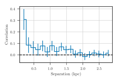
Figure 9: Two-point correlation function of the GMC positions from Corbelli et al. (2017) measured in 150 pc bins. The uncertainties are estimated from 2000 bootstrap iterations. Most of the correlation occurs on $<150$ pc scales, but the structure of CO emission due to the disk gives non-zero correlations up to $\sim 2$ kpc scales.

This result may also explain the large change in the CO power-spectrum index across the $\sim 120$ pc break point found by Combes et al. (2012). Distinct breaks in the power-spectra, and other turbulent metrics, are useful probes of the disk scale height (Elmegreen et al., 2001; Padoan et al., 2001). The power-spectrum index is predicted to change by $+1$ on scales larger than the disk scale height since large-scale turbulent motions are confined to two dimensions in the disk (Lazarian & Pogosyan, 2000). Combes et al. (2012) find the CO power-spectrum index changes by $+2.2$ across the break, significantly larger than the expected change of $+1$. For the H i, the index change of $+0.8$ across the break is much closer to the expected change.

The similarity Combes et al. (2012) find between the CO and H i break points in the power-spectra also differs from the disk scale heights implied by the line widths we find. For ratios $\sigma_{\rm CO}/\sigma_{\rm HI}<1$, the disk scale height of CO should be smaller than the H i; we can approximate the ratio of the disk scale heights from the line width ratio. For $R_{\rm gal}<7$ kpc, the stellar surface density is larger than the total gas surface density in M33 (Corbelli et al., 2014). Measurements of the stellar velocity dispersion find $\sim 20$ ${\rm km\,s^{-1}}$ in the inner disk (Kormendy & McClure, 1993; Gebhardt et al., 2001; Corbelli, 2003), suggesting the stellar disk scale height is larger than the H i and CO disk scale heights. If this result holds true for $R_{\rm gal}<7$ kpc, the ratio of the CO and H i disk scale heights is the ratio of the line widths: $H_{\rm CO}/H_{\rm HI}\approx\sigma_{\rm CO}/\sigma_{\rm HI}$ (Combes & Becquaert, 1997), for line widths measured at the disk scale height. Based on our analysis at $80$ and $160$ pc, the line width ratio is $\sim 0.6$, suggesting that the CO scale height should be $\sim 60\%$ of the H i scale height.

The discrepancy with the scale heights we measure and the similar scale of the break points from Combes et al. (2012) may be a limitation of the data resolution used in their analysis. They use H i and CO data at $12\arcsec$ ($\sim 50$ pc) resolution (Gratier et al., 2010) and the constraints on the scale of the break are limited by the beam size, as shown in their Appendix B. Higher resolution observations ($\sim 20$ pc) should determine whether there is a difference in the disk scale heights traced by H i and CO.

4.2 Similarities with the flocculent spiral NGC 2403

From the sample of nearby galaxies studied in Caldu-Primo et al. (2013), there are two galaxies that are also dominated by the atomic component throughout most of the disk: NGC 925 and NGC 2403 (see also Schruba et al., 2011). As these are the closest analogs to M33 in their sample, we compare the stacked profile analyses from Caldu-Primo et al. (2013) to our results.

The NGC 925 line width ratios are consistent with unity, however, the signal-to-noise in the CO map limit the analysis to a few radial bins at the galaxy centre. The signal-to-noise of the NGC 2403 data is higher, allowing the analysis to be extended to larger radii ($70\%$ of the optical radius) providing a number of radial bins for comparison. NGC 2403 is also the closest galaxy in their sample and the physical scale of the beam is ${\sim}200$ pc, a factor of about two coarser than the resolution of our M33 data. Interestingly, the line width ratios, outside of the galactic centre (${\sim}0.1R_{25}$), are consistently smaller than unity, with an average of ${\sim}0.8$. The increased line widths in the inner disk are likely affected by beam smearing. With the same data, the line-of-sight analysis by Mogotsi et al. (2016) find a smaller line width ratio of ${\sim}0.7$. Both of these line width ratios are comparable to our results in M33 on $160$ pc ($38\arcsec$) scales. Our results are then consistent with the ratios for NGC 2403 from Caldu-Primo et al. (2013) and Mogotsi et al. (2016), suggesting that galaxies with atomic-dominated neutral gas components have at most a moderate contribution from a diffuse molecular disk.

5 Summary

We explore the spectral relationship of the atomic and molecular medium in M33 on 80 pc scales by comparing new VLA H i observations (K18) with IRAM 30-m CO(2-1) data (Gratier et al., 2010; Druard et al., 2014). We perform three analyses—the difference in the velocity at peak H i and CO(2-1) brightness, spectral stacking, and fits to individual spectra—to explore how the atomic and molecular ISM are related. Each of these analyses demonstrates that the spectral properties between the H i and CO are strongly correlated on $80$ pc scales. We also show that relationship between the H i and CO line widths, on $80$ pc scales, from individual spectral fits depend critically on identifying the H i most likely associated with CO emission, rather than all H i emission along the line-of-sight.

1. The velocities of the H i and CO peak temperatures are closely related. The standard deviation in the differences of these velocities is $2.7$ ${\rm km\,s^{-1}}$, slightly larger than the CO channel widths ($2.6$ ${\rm km\,s^{-1}}$; Figure 2). Significant outliers in the velocity difference ($>10$ ${\rm km\,s^{-1}}$) occur where the H i spectrum has multiple components and the CO peak is not associated with the brightest H i peak. These outliers are removed when modelling only the H i component associated with CO (§3.3).

2. By stacking H i and CO spectra aligned to the velocity of the peak H i brightness, we find that the width of the CO stacked profile ($4.6\pm 0.9$ ${\rm km\,s^{-1}}$) is smaller than the H i stacked profile ($6.6\pm 0.1$ ${\rm km\,s^{-1}}$) on 80 pc scales, unlike similar analyses of other (more massive) nearby galaxies that measure comparable line widths on 500 pc scales (e.g., Caldu-Primo et al., 2013). The widths of the stacked profiles slowly decrease with galactocentric radius.

3. By repeating the stacking analysis at lower spatial resolutions of 160 pc ($38\arcsec$) and 380 pc ($95\arcsec$), we find that the CO(2-1)-to-H i line width ratio remains constant within uncertainty. We estimate how beam smearing contributes at each resolution and find that resolutions of 80 and 160 pc have a similar contribution to the line width from beam smearing. Beam smearing contributes more at a resolution of 380 pc and can explain the increased line widths relative to those at 160 pc. However, the CO line width remains smaller than the H i on all scales.

4. We perform a spectral decomposition of H i spectra limited to where CO is detected. The CO spectra are fit by a single Gaussian, while the Gaussian fit to the H i is limited to the closest peak in the H i spectrum. We carefully inspect and impose restrictions to remove spectra where this fitting approach is not valid. The average H i and CO line widths of the restricted sample are $7.4^{+1.7}_{-1.3}$ and $4.3^{+1.5}_{-1.0}$ ${\rm km\,s^{-1}}$, where the uncertainties are the 15^th and 85^th percentiles of the distributions, respectively.

5. The average CO line width from the line-of-sight fits are smaller than those from the stacking analysis. This difference results from aligning the CO spectra to the H i peak velocity, while there is scatter between the H i and CO velocity at peak intensity (Figure 2). Recovering larger CO stacked line widths relative to those from individual spectra is a general result that will result whenever CO is aligned with respect to another tracer, such as H i. The amount of line broadening is set by the scatter between the line centres of the two tracers. Thus, line stacking based on a different tracer will bias the line widths to larger values, but is ideal for recovering faint emission (Schruba et al., 2011).

6. The average H i line width from the line-of-sight fits ($7.4\pm 1.5$ ${\rm km\,s^{-1}}$) is larger than the stacked profile width ($6.6\pm 0.1$ ${\rm km\,s^{-1}}$). The larger line widths are due to either multiple highly-blended Gaussian components that are not modelled correctly in our analysis, or that the H i associated with CO emission tends to have larger line widths. We favour the latter explanation since our line-of-sight analysis has strong restrictions to remove multi-component spectra (Appendix C); however, we do not fully decompose the H i spectra and cannot rule out the former explanation.

7. The line-of-sight fits highlight a strong correlation between H i and CO line widths (Figure 6). We fit for the line width ratio, accounting for errors in both measurements, and find $\sigma_{\rm CO}=(0.56\pm 0.01)\ \sigma_{\rm HI}$, smaller than the ratios from the stacked profiles due to the smaller average CO line width and larger average H i line width. There is no trend between the line width ratio and galactocentric radius (Figure 8). When repeated at a lower spatial resolution, we find that the H i and CO line widths are increased by the same factor, leading to the same line width ratio, within uncertainties.

8. The scatter in the relation between the H i and CO line widths is larger than the statistical errors and results from regional variations (Figure 7). The line widths of H i and CO remain correlated when measured in individual regions, but exhibit systematic offsets with respect to the median H i and CO line widths. These regional variations affect both the H i and CO line widths and suggest that the local environment plays an important role in setting the line widths.

9. We perform stacking tests with the fitted LOS components to constrain sources of the line wing excess. We find that the error beam pick-up from the IRAM 30-m telescope (Druard et al., 2014) and systematics of the stacking procedure can account for $\sim 80$% of the line wing excess in the CO(2-1) (§3.4.3). Combined with a CO-to-H i line width ratio less than unity, this result implies that M33 has at most a marginal thick molecular disk. We point out that previous analyses of NGC 2403 give similar results to ours (Caldu-Primo et al., 2013; Mogotsi et al., 2016), suggesting that galaxies where the atomic component dominates the cool ISM may lack a significant thick molecular disk.

Scripts to reproduce the analysis are available at https://github.com/Astroua/m33-hi-co-lwidths.

Appendix A Line Broadening from Beam Smearing

Spectral line widths can be broadened wherever there is a large gradient in the rotation velocity on scales of the beam size. This line broadening, commonly referred to as beam smearing, tends to have the largest effect near the centres of galaxies, where the rotation curve is steep, and can lead to significant increases in the line width of stacked profiles (e.g., Stilp et al., 2013; Ianjamasimanana et al., 2015; Caldú-Primo et al., 2015).

We require constraints on beam smearing when comparing line widths measured at different spatial resolutions in our data to distinguish whether broadened line profiles are the result of physical processes. We estimate the maximum broadening from beam smearing by using a rolling tophat filter on the peak H i velocity map to calculate the standard deviation over one beam. This operation measures the beam-to-beam variation in the peak velocity field. We note that these variations may not be entirely due to beam smearing and could arise from local variations in velocity, such as those measured for molecular cloud and envelope rotation in the H i (Imara et al., 2011). Therefore, our estimates are an upper limit on line broadening due to beam smearing. This is a similar measurement to the approach used by Caldú-Primo & Schruba (2016), where they measure the width of the velocity distribution on local scales along the major and minor axes of M31.

We compute the standard deviation in the peak H i velocity surface at the original (80 pc/$20\arcsec$) and degraded resolutions (160 pc/$38\arcsec$ and 380 pc/$95\arcsec$) used in Sections 3.2 & 3.3. Since large-scale variations in the peak H i velocity describe the circular rotation curve, we calculate the average values of the standard deviation surfaces in $0.5$ kpc galactocentric radial bins. If beam smearing significantly broadens the line, we expect the profile of average values to follow the derivative of the circular rotation curve, which is steepest within the inner 2 kpc of M33 (K18). Figure 10 shows the average of the standard deviation surfaces at the three different beam sizes used for the analysis. The average radial profiles for beam widths of 80 and 160 pc do not have strong radial trends and show that beam smearing contributes at most $\sim 2$ ${\rm km\,s^{-1}}$ to the line width. We calculate the area-weighted average of the radial profiles in Figure 10 and find values of $2.0^{+2.1}_{-1.8}$ ${\rm km\,s^{-1}}$ and $1.5^{+1.7}_{-0.8}$ ${\rm km\,s^{-1}}$ for beam sizes of 80 and 160 pc, respectively. The uncertainties quoted here are the $15^{\rm th}$ and $85^{\rm th}$ percentiles of the radial profiles with the same area-weighted averaging applied. Since the CO(2-1) channel width is $2.6$ ${\rm km\,s^{-1}}$, the line width broadening of CO(2-1) from beam smearing is similar to the correction factor for the channel width.

Using the average line-of-sight CO line width of $4.3$ ${\rm km\,s^{-1}}$ at a resolution of 80 pc (Table 2), the correction due to beam smearing gives a $\sim 10$% in the line width.

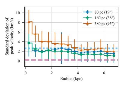
Figure 10: Average standard deviations from the peak H i velocity map measured over one beam. Three average curves are shown measured within $0.5$ kpc bins at the original beam size (80 pc/$20\arcsec$; blue circles), and at twice (160 pc/$38\arcsec$; green diamonds) and five times (380 pc/$95\arcsec$; orange triangles) the original beam size. Error bars correspond to the standard deviation within each bin, uncorrected for the number of independent samples to demonstrate where the distributions are consistent with $0$ ${\rm km\,s^{-1}}$. The thick, horizontal lines correspond to the H i (pink dashed; $0.2$ ${\rm km\,s^{-1}}$) and CO(2-1) (cyan dotted; $2.6$ ${\rm km\,s^{-1}}$) channel widths. The average values represent the maximum line broadening that could result from beam smearing. Line widths at resolutions of 80 and 160 pc are uniformly broadened by $\sim 2$ ${\rm km\,s^{-1}}$, while the broadening at a resolution of 380 pc is $\sim 3$ ${\rm km\,s^{-1}}$ and increases to $8$ ${\rm km\,s^{-1}}$ in the inner kpc.

The average standard deviation profile measured at a beam size of 380 pc ($95\arcsec$) shows a strong radial trend within the inner 4 kpc, as expected from beam smearing. The broadening from beam smearing is particularly strong within $R_{\rm gal}<2$ kpc, where the maximum average standard deviation is $\sim 8.2$ ${\rm km\,s^{-1}}$. The area-weighted average, as applied to the higher resolution measurements, is $2.8^{+1.0}_{-1.0}$ ${\rm km\,s^{-1}}$. Subtracting this mean value in quadrature from the 380 pc stacked line widths (Table 1) gives corrected line widths of $8.4\pm 0.9$ ${\rm km\,s^{-1}}$ for H i and $6.7\pm 3.6$ ${\rm km\,s^{-1}}$ for CO(2-1). The CO(2-1) is not constraining due to the uncertainty from the channel width, however the H i line width range demonstrates that the $0.9$ ${\rm km\,s^{-1}}$ increase in the line width between the 160 and 380 pc data can entirely be explained by beam smearing.

Appendix B Forward-modelling the spectral response function

We forward-model the individual LOS fits to the CO data in §3.3 with an approximation for the spectral response function. Here, we briefly describe the fitting process.

We approximate the spectral response function in the CO(2-1) IRAM-30m data based on the nearest neighbour channel correlation found by Sun et al. (2018, $r=0.26$ for scales $>70$ pc, adjusted to a distance of 840 kpc used here). Using the empirically-derived relation from Leroy et al. (2016), this correlation corresponds to a channel-coupling factor of $k=0.11$ for a three-element Hann-like kernel ($[k,1-2k,k]$), which we adopt as the spectral response function.

We forward-model the spectral response in two steps:

1. The Gaussian model is sampled at the spectral channels of the observed spectra. This sampling is equivalent to taking the weighted average of the Gaussian over the spectral channel width ($\Delta v$):

   $$G(v)=\frac{A}{(\Delta v)^{2}}\left[{\rm erf}\left(\frac{\mu-(v-\Delta v/2)}{\sqrt{2}\sigma}\right)-{\rm erf}\left(\frac{\mu-(v+\Delta v/2)}{\sqrt{2}\sigma}\right)\right],$$ (5)

   for a Gaussian centered at velocity $\mu$ with an amplitude of $A$ and width of $\sigma$ that is averaged over channels centered at $v$. The channel averaging is equivalent to convolving the Gaussian with a top-hat kernel with a width of $\Delta v$.

2. The Gaussian sampled over the spectral channels is convolved with the Hann-like kernel described above. This step accounts for the measured channel correlations in the observations.

The sampled and convolved spectrum is then compared to the observed spectrum and the sum of the squared distances is the quantity minimized in the fit. Using this approach removes biases in the fitted line width parameters (Koch et al., 2018a). This approach is similar to the forward-modelling in Rosolowsky et al. (2008).

We note that the non-linear least-squares fit used in this paper assumes that the data uncertainties are independent, which is not true due to the spectral-response of the data. To test whether the parameter uncertainties from the covariance matrix of the fit are underestimated due to being correlated, we repeat the fitting procedure on 1000 simulated spectra sampled with channel widths of $\Delta v=\sigma$. White-noise is added to the spectra then convolved with the Hann-like kernel to give a peak S/N of 5. We find that $\sim 72\%$ of the fitted parameters are within the $1\mbox{--}\sigma$ uncertainty interval. This is similar to the expected $68.2\%$ expected for a two-tailed p-test, demonstrating that the parameter uncertainties are not underestimated despite the correlated errors.

Appendix C Validating the Gaussian Decomposition

We demonstrate our limited Gaussian decomposition method (§3.3) and perform two validation checks on the sample used in the analysis.

The first check compares the surface densities from the integral over the fitted Gaussian model to the integrated intensity of the data located within the model’s FWHM, scaled by $1/{\rm erf}(\sqrt{2})$ to account for emission outside of the mask. Figure 11 shows excellent agreement between the two methods for the H i and CO fits. This implies that the peaks are well-described by a Gaussian and validates the choice of model.

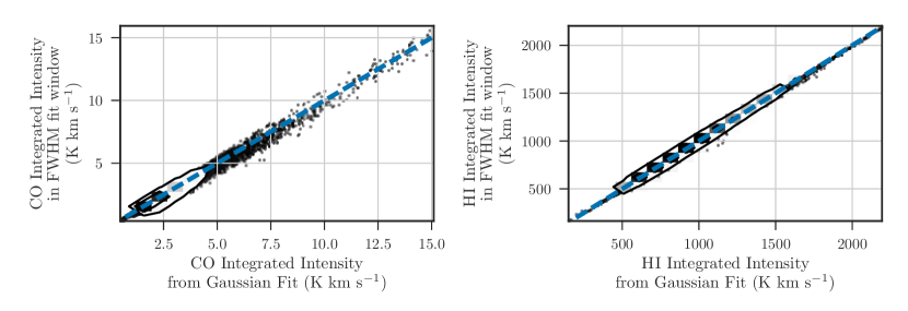
Figure 11: The CO (left) and H i (right) integrated intensities from the spectra within the FWHM window used for the fit ($y$-axis) compared with the integral over the fitted Gaussian models ($x$-axis). The blue-dashed line is the line of equality. There is little deviation from the line of equality, indicating that the Gaussian models describe the data within the FWHM fitting windows well.

The second validation check is a comparison of the integral over the fitted Gaussian model with respect to the integrated intensities over the whole profile. Figure 12 shows these quantities for the CO and H i. For the CO integrated intensities, there is no significant variation between the two quantities. This is expected, since we require that the CO profiles be well-fit by a Gaussian in order to be in the sample. The discrepancy between these quantities for the H i is larger. Again, this is expected, since the masking used in the H i fitting is introduced to remove spectral features unlikely to be associated with the CO component.

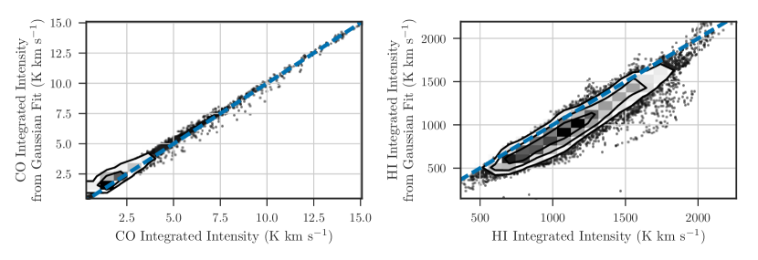
Figure 12: The CO (left) and H i (right) integrated intensities from the integral over the fitted Gaussian models ($y$-axis) compared to the integrated intensity over the whole spectra ($x$-axis). The blue-dashed line is the line of equality. There remains good agreement for the CO spectra, however the H i integrated intensity from the Gaussian fit is consistently smaller the from the entire spectra due to the additional H i line structure.

With these two checks, we are confident that the clean sampled used for the analysis describes only single-peaked CO profiles and H i profiles with a well-defined peak associated with the CO emission.

C.1 Effect of H i Masking on Fitting

We investigate how the FWHM mask affects the fitted H i line width by repeating the fitting without the mask. This procedure has been used in other studies relating H i and CO line profiles from individual spectra (Fukui et al., 2009; Mogotsi et al., 2016). For H i profiles with multiple components or prominent line wings, we expect that the fitted profiles without masking will be much wider. Figure 13 shows that most H i profiles are indeed wider without the masking, with the median width increasing from $7.4$ to $8.3$ ${\rm km\,s^{-1}}$. This result highlights the need to carefully disinguish bright H i emission from extended line wings to avoid biasing the H i line widths and reinforces the use of the upper-limit of $12$ ${\rm km\,s^{-1}}$ in $\sigma_{\rm HI}$ set here to minimize contamination in our sample.

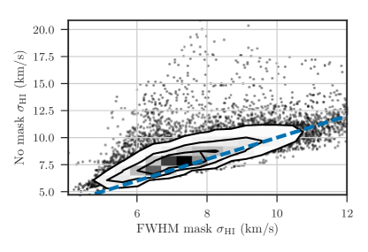
Figure 13: H i line widths fit with and without a FWHM mask around the peak. The contours represent the 2- to 4-$\sigma$ limits of the population, and points outside the contours are outliers beyond 4-$\sigma$. The blue-dashed line indicates equality between the line widths.

C.2 Examples of Fitted Spectra

In Figures 14 and 15, we demonstrate fitted H i and CO spectra and how our criteria for the analysis sample removes clear issues. Figure 14 is an example of a valid fit to both H i and CO, while Figure 15 demonstrates a poor fit that is excluded from the analysis.

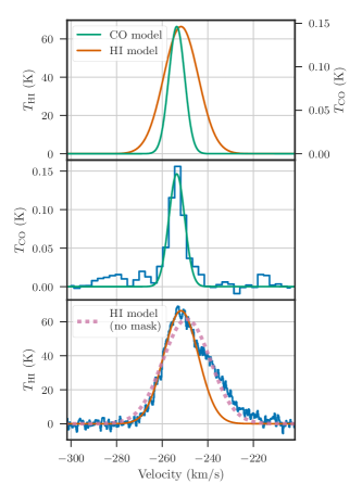
Figure 14: Example of the H i and CO Gaussian fitting showing well-fit single components that are included in our clean sample. The top panel shows the fitted H i and CO profiles. The middle panel shows the CO spectrum with the fit overlaid. The bottom panel shows the same for the H i data, and also includes a fit to the H i data if no masking is applied when fitting (thick-dashed line; §C.1). The H i fit the brightest peak is significantly improved when masking is used.

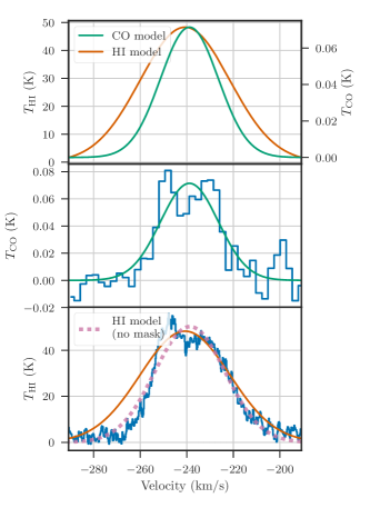
Figure 15: Same as Figure 14. This example shows failed fits in both tracers due to multiple-components and is rejected from the clean sample. There appears to be two Gaussians in both spectra and fitting a multi-Gaussian model should distinguish between the two. Extending this analysis to multi-component spectra will be the focus of future work.

Appendix D Stacked Profile Widths

Table 4 shows the stacked line widths ($\sigma_{\rm HWHM}$) in radial bins. These line widths are plotted in the top panel of Figure 4 and described in §3.2.1.

Table 4: HWHM line widths ($\sigma_{\rm HWHM}$) for the H i and CO(2-1) stacked profiles in 500 pc radial bins at 80 pc resolution. The uncertainties are propagated assuming an uncertainty of half the channel width and the uncertainty of each point in the spectrum is the standard deviation of values within that channel scaled by the square-root of the number of beams.

$R_{\rm gal}$ (kpc)	$\sigma_{\rm HI}$ (${\rm km\,s^{-1}}$)	$\sigma_{\rm CO}$ (${\rm km\,s^{-1}}$)
$0.0\mbox{--}0.5$	$8.0\pm 0.1$	$5.0\pm 0.9$
$0.5\mbox{--}1.0$	$7.3\pm 0.1$	$4.6\pm 1.0$
$1.0\mbox{--}1.5$	$6.9\pm 0.1$	$4.5\pm 1.0$
$1.5\mbox{--}2.0$	$7.3\pm 0.1$	$4.8\pm 0.9$
$2.0\mbox{--}2.5$	$7.4\pm 0.1$	$4.8\pm 0.9$
$2.5\mbox{--}3.0$	$7.4\pm 0.1$	$4.7\pm 0.9$
$3.0\mbox{--}3.5$	$6.8\pm 0.1$	$4.7\pm 0.9$
$3.5\mbox{--}4.0$	$7.2\pm 0.1$	$4.8\pm 1.0$
$4.0\mbox{--}4.5$	$6.7\pm 0.1$	$4.4\pm 1.0$
$4.5\mbox{--}5.0$	$6.9\pm 0.1$	$4.6\pm 1.0$
$5.0\mbox{--}5.5$	$6.9\pm 0.1$	$4.1\pm 1.0$
$5.5\mbox{--}6.0$	$6.9\pm 0.1$	$3.9\pm 0.9$
$6.0\mbox{--}6.5$	$6.6\pm 0.1$	$4.3\pm 1.0$
$6.5\mbox{--}7.0$	$6.1\pm 0.1$	$3.8\pm 1.1$

References

- Astropy Collaboration et al. (2013) Astropy Collaboration et al., 2013, Astronomy & Astrophysics, 558, A33
- Bialy et al. (2017) Bialy S., Burkhart B., Sternberg A., 2017, ApJ, 843, 92
- Bigiel et al. (2008) Bigiel F., Leroy A., Walter F., Brinks E., de Blok W. J. G., Madore B., Thornley M. D., 2008, AJ, 136, 2846
- Blitz & Rosolowsky (2006) Blitz L., Rosolowsky E., 2006, ApJ, 650, 933
- Bolatto et al. (2011) Bolatto A. D., et al., 2011, ApJ, 741, 12
- Braine et al. (2018) Braine J., Rosolowsky E., Gratier P., Corbelli E., Schuster K. F., 2018, A&A, 612, A51
- Braun (1997) Braun R., 1997, ApJ, 484, 637