On the Assouad dimension of projections

Abstract.

Let $F\subset\mathbb{R}^{2}$, and let $\dim_{\textsc{A}}$ stand for Assouad dimension. I prove that

$$\dim_{\textsc{A}}\pi_{e}(F)\geq\min\{\dim_{\textsc{A}}F,1\}$$

for all $e\in S^{1}$ outside of a set of Hausdorff dimension zero. This is a strong variant of Marstrand’s projection theorem for Assouad dimension, whose analogue is not true for other common notions of fractal dimension, such as Hausdorff or packing dimension.

1. Introduction

1.1. The main result and previous work

For $F\subset\mathbb{R}^{2}$, let $\dim_{\textsc{A}}F$ be the Assouad dimension of $F$, see Definition 3.1. For $e\in S^{1}$, write $\pi_{e}\colon\mathbb{R}^{2}\to\mathbb{R}$ for the projection map $\pi_{e}(x)=x\cdot e$. Here is the main result of the paper:

Theorem 1.1.

Let $F\subset\mathbb{R}^{2}$. Then,

$$\dim_{\mathrm{H}}\{e\in S^{1}:\dim_{\textsc{A}}\pi_{e}(F)<\min\{\dim_{\textsc{A}}F,1\}\}=0.$$

Theorem 1.1 improves on an earlier result of Fraser and the author [10, Theorem 2.1], where it was proven that

$$\mathcal{H}^{1}(\{e\in S^{1}:\dim_{\textsc{A}}\pi_{e}(F)<\min\{\dim_{\textsc{A}}F,1\})=0.$$ (1.2)

To put Theorem 1.1 into proper context, I briefly list below the main existing projection theorems concerning a general compact set $K\subset\mathbb{R}^{2}$, and I also discuss their sharpness.

Hausdorff dimension

Let $\dim_{\mathrm{H}}$ stand for Hausdorff dimension. Marstrand in 1954, see [20, Theorem II], proved that the set

$$E:=E(K):=\{e\in S^{1}:\dim_{\mathrm{H}}\pi_{e}(K)<\min\{\dim_{\mathrm{H}}K,1\}\}$$

has $\mathcal{H}^{1}(E)=0$. In 1968, Kaufman [18] improved this in the case $\dim_{\mathrm{H}}K<1$ by showing that $\dim_{\mathrm{H}}E\leq\dim_{\mathrm{H}}K$. Kaufman’s bound is sharp in the following sense: Kaufman and Mattila [17, Theorem 5] constructed a compact set $K\subset\mathbb{R}^{2}$ with any Hausdorff dimension $\dim_{\mathrm{H}}K\in[0,1]$ such that $\dim_{\mathrm{H}}E=\dim_{\mathrm{H}}K$.

Packing and box dimensions

Let $\dim_{\mathrm{p}}$ stand for packing dimension. Then, there are compact sets $K\subset\mathbb{R}^{2}$ such that

$$\{e\in S^{1}:\dim_{\mathrm{p}}\pi_{e}(K)<\min\{\dim_{\mathrm{p}}K,1\}\}=S^{1}.$$

Such sets were first constructed by Järvenpää [15]. However, positive results can be obtained by considering instead $\{e\in S^{1}:\dim_{\mathrm{p}}\pi_{e}(K)<s\}$ for various $0<s<\dim_{\mathrm{p}}K$. For sharp results, both positive and negative, see the work [5] of Falconer and Howroyd. The situation is similar for box dimension(s), see the references above.

Assouad dimension

Theorem 1.1 evidently gives a sharp result for Assouad dimension, although one could further ask if

$$\dim_{\mathrm{p}}\{e\in S^{1}:\dim_{\textsc{A}}\pi_{e}(K)<\min\{\dim_{\textsc{A}}K,1\}\}=0.$$

The proof in this paper does not seem to give this improvement. It would also be interesting to know if $\{e\in S^{1}:\dim_{\textsc{A}}\pi_{e}(K)<\min\{\dim_{\textsc{A}}K,1\}\}$ can be uncountable.

Theorem 1.1 does not imply that $\dim_{\textsc{A}}\pi_{e}(K)=\min\{\dim_{\textsc{A}}K,1\}$ for all $e\in S^{1}$ outside of a small set of exceptions. In fact, such a statement is far from true. It was already observed in [10] that the map $e\mapsto\dim_{\textsc{A}}\pi_{e}(K)$ can be essentially non-constant. This observation was recently strengthened by Fraser and Käenmäki [9]: if $\phi\colon S^{1}\to[0,1]$ is any upper semicontinuous function with $\phi(e)=\phi(-e)$, then there exists a compact set $K\subset\mathbb{R}^{2}$ with $\dim_{\textsc{A}}K=0$ such that $\dim_{\textsc{A}}\pi_{e}(K)=\phi(e)$ for all $e\in S^{1}$.

A mixed problem

What about the set

$$E^{\prime}:=\{e\in S^{1}:\dim_{\mathrm{p}}\pi_{e}(K)<\min\{\dim_{\mathrm{H}}K,1\}\}?$$

Since packing dimension an upper bound for Hausdorff dimension, the theorems of Kaufman and Marstrand imply that $\mathcal{H}^{1}(E^{\prime})=0$ and $\dim_{\mathrm{H}}E^{\prime}\leq\dim_{\mathrm{H}}K$. This is unlikely to be sharp: I am not aware of a compact set $K\subset\mathbb{R}^{2}$ with $\dim_{\mathrm{H}}E^{\prime}>0$! In contrast, $\dim_{\mathrm{p}}E^{\prime}$ can take values arbitrarily close to $1$, see [22, Theorem 1.17].

Sets with additional structure

If $K\subset\mathbb{R}^{2}$ is self-similar, then

$$\dim_{\mathrm{p}}\{e\in S^{1}:\dim_{\mathrm{H}}\pi_{e}(K)<\min\{\dim_{\mathrm{H}}K,1\}\}=0.$$ (1.3)

This is a result of Hochman [14, Theorem 1.8] in the case where $K$ contains no irrational rotations. In the presence of irrational rotations, one can further improve (1.3) to

$$\{e\in S^{1}:\dim_{\mathrm{H}}\pi_{e}(K)<\min\{\dim_{\mathrm{H}}K,1\}\}=\emptyset,$$ (1.4)

which is an earlier result of Peres and Shmerkin [23]. Under suitable irrationality hypotheses, too lengthy to explain here, the conclusion (1.4) is also known for self-conformal sets [4], and several classes of self-affine sets, see [7, 1].

1.2. Outline of the proof

Before explaining the main steps in the proof of Theorem 1.1, I need to describe two initial reductions.

1.2.1. Initial reductions

First, since Assouad dimension is invariant under taking closures, it suffices to prove Theorem 1.1 for closed sets $F$. Second, it suffices to prove Theorem 1.1 for compact sets $F\subset\mathbb{R}^{2}$ with $\mathcal{H}^{\dim_{\textsc{A}}F}(F)>0$. The proof of this reduction is the same as the proof of [8, Theorem 2.9], but I sketch the idea briefly; see [8] for more details. By a result of Käenmäki, Ojala, and Rossi [16, Proposition 5.7], any closed set $F\subset\mathbb{R}^{2}$ has a weak tangent $E\subset\mathbb{R}^{2}$ with $\dim_{\textsc{A}}E=\dim_{\mathrm{H}}E=\dim_{\textsc{A}}F$, and even

$$\mathcal{H}^{\dim_{\textsc{A}}E}(E)>0.$$ (1.5)

The authors of [16] omit mentioning (1.5), but this is what they prove (see also the discussion after [8, Theorem 1.3]). Now, for any $e\in S^{1}$, the projection $\pi_{e}(E)$ turns out to be a subset of some weak tangent $W_{e}$ of $\pi_{e}(F)$ (see the proof of [8, Theorem 2.9] for details), and hence

$$\dim_{\textsc{A}}\pi_{e}(F)\geq\dim_{\textsc{A}}W_{e}\geq\dim_{\textsc{A}}\pi_{e}(E)$$

where the first inequality is [19, Proposition 6.1.5]. Consequently,

$$\{e\in S^{1}:\dim_{\textsc{A}}\pi_{e}(F)<\min\{\dim_{\textsc{A}}F,1\}\}\subset\{e\in S^{1}:\dim_{\textsc{A}}\pi_{e}(E)<\min\{\dim_{\textsc{A}}E,1\}\},$$

and Theorem 1.1 now follows if one manages to prove that the set on the right has zero Hausdorff dimension. Recalling that $E$ satisfies (1.5), this completes the proof of the second reduction.

1.2.2. The main argument

Let $F\subset\mathbb{R}^{2}$ be a compact set satisfying $\mathcal{H}^{d}(F)>0$, where $d:=\dim_{\textsc{A}}F$. These are reasonable assumptions by the previous discussion. Then, let $\mu$ be a $d$-dimensional Frostman measure supported on $F$, and assume with no loss of generality that $F=\operatorname{spt}\mu$. The measure $\mu$ is not quite $d$-regular, but not too far from it either, precisely because $\dim_{\textsc{A}}F$ matches the Frostman exponent of $\mu$. For a way to quantify this, see Lemma 3.8.

The measure $\mu$ itself is still too general to work with, so we need to pass to another tangent $\nu=\mu^{B}$, where $B$ is a ball with $\mu(B)\approx\operatorname{diam}(B)^{d}$. Most balls have this property by the near-$d$-regularity of $\mu$. To list the (less trivial) properties required of $\nu$, start with a counter assumption: $\dim_{\mathrm{H}}S>\epsilon>0$, where $S=\{e:\dim_{\textsc{A}}\pi_{e}(F)<D\}$ and $0<D<\min\{1,d\}$. Then, locate an $\epsilon$-dimensional Frostman measure $\sigma$ on $S$. The properties needed of $\nu$ are now – very roughly speaking! – the following: there is a constant $0\leq s\leq D$ such that

• $\pi_{e}(\nu)$ is exact dimensional with dimension $s$ for $\sigma$ almost every $e\in S$,

• The projections $\pi_{e}$ are dimension conserving relative to $\nu$ (in the sense of Furstenberg [11]) for $\sigma$ almost every $e\in S$.

The second requirement means that the measure $\nu$ conditioned on a $\pi_{e}(\nu)$-generic fibre $\pi_{e}^{-1}\{x\}$ is at least $(d-s)$-dimensional. It is possible that a tangent $\nu=\mu^{B}$ satisfying (a)-(b) literally could be extracted by the theory of CP-chains, see [11, Section 6], [13, Theorem 1.22], and [13, Theorem 1.30]. However, the requirements (a)-(b) should not be interpreted literally: what we really need are certain $\delta$-discretised versions of (a)-(b); for a precise statement (which is admittedly difficult to decipher with the current background), see (K1)-(K2) in Section 4.2. So, instead of applying the theory of CP-chains, the proof below only relies on combinatorial argument, notably the pigeonhole principle.

After $\nu$ has been found, we start looking for a contradiction to the hypothesis that $\dim_{\mathrm{H}}\sigma>0$. This constitutes the main effort in the paper. Note that $\nu=\mu^{B}$ is still near-$d$-regular, because $\mu(B)\approx\operatorname{diam}(B)^{d}$, and $\dim_{\textsc{A}}F=d$. So, what we roughly need to prove is the following:

Conjecture 1.6.

Assume that $\nu$ is a near-$d$-regular measure on $\mathbb{R}^{2}$, $0\leq s<d$, and $\sigma$ is a Borel probability measure on $S^{1}$ such that (a)-(b) are satisfied. Then $\dim_{\mathrm{H}}\sigma=0$.

Conjecture 1.6 seems plausible, but I do not claim to prove it here. In fact, recalling that the our $\nu$ only satisfies approximate variants of (a)-(b), Conjecture 1.6 would not be literally useful in the present context. However, the underlying point in Section 4.3 is to prove a version of Conjecture 1.6, using the "real" information we have about $\nu$, and hence contradict the positive-dimensionality of $\sigma$.

To be honest, this "real" information contains some pieces not contained in (a)-(b). First, we have $S\subset\{e:\dim_{\textsc{A}}\pi_{e}(F)<D\}$, which in particular implies a quantitative – and useful – porosity property for $\operatorname{spt}\pi_{e}(\nu)$, $e\in S$. With additional effort, one might be able to work with the weaker measure-theoretic porosity of $\pi_{e}(\nu)$ implied by (a) alone, but the set-theoretic porosity of $\operatorname{spt}\pi_{e}(\nu)$ is certainly more pleasant to apply. A second, and more crucial, piece of additional information is

• property (a) also for all tangents of $\nu$ of "at moderate scales".

This roughly means that if $\delta>0$ is the smallest scale where all the action happens, and $\delta<\Delta\leq\delta^{\kappa}$ for some suitable (small) constant $\kappa=\kappa(\epsilon)>0$, then the renormalised restriction of $\nu$ to any $\Delta$-ball centred at $\operatorname{spt}\nu$ has roughly $s$-dimensional projections at scale $\delta/\Delta$ for most directions $e\in S$. This is vital in Section 4.3, but makes virtually no difference in the construction of $\nu$. I do not know how to derive – or even formulate – an analogous statement from/within the theory of CP-chains.

At the end, the proof of our (discretised and watered-down version of) Conjecture 1.6 rests on an application of Shmerkin’s inverse theorem [24, Theorem 2.1]. This theorem is the latest quantification of the following phenomenon, initially discovered by Bourgain [2, 3], and later developed by Hochman [14]: if $\nu_{1}\times\nu_{2}$ is a product measure on $\mathbb{R}^{2}$, $e\in S^{1}$ is at positive distance from $\{(1,0),(0,1)\}$, and the $\delta$-entropies of $\pi_{e}(\nu_{1}\times\nu_{2})$ and $\dim\nu_{1}$ are comparable for some $0<\delta\ll 1$, then all the scales between $\delta$ and $1$ can be split into two disjoint groups: those where $\nu_{1}$ is "uniform", and those where $\nu_{2}$ is "singular".

In our setting, there are no product measures to begin with. However, assuming that $(1,0)\in S$ without loss of generality, a scheme introduced in [21] allows one to derive from $\nu$ – using (a’) – a product measure $\nu_{1}\times\nu_{2}$ with the properties that

1. $\nu_{1}\approx\pi_{(1,0)}(\nu)$,

2. $\nu_{2}\approx\nu$ conditioned on a $\pi_{(1,0)}(\nu)$-generic fibre $\pi_{(1,0)}^{-1}\{x\}$,

3. $\dim\pi_{e}(\nu_{1}\times\nu_{2})\approx\dim\pi_{e}(\nu)$ for $e\in S$ sufficiently close to $(1,0)$.

This step is accomplished in Sections 4.4-4.5. The main geometric idea is that if $\delta>0$ is a scale, $T=J\times[0,1]\subset[0,1]^{2}$ is a vertical $\delta^{1/2}$-tube, where $J\subset[0,1]$ is a $\delta^{1/2}$-interval, and $P\subset T$ is any $\delta$-separated set, then there always exists a "quasi-product" set $\bar{P}\subset T$ of the form

$$\bar{P}=\bigcup_{h\in\mathcal{D}}\bar{P}_{h}\times\{h\}$$

such that the $\delta$-covering numbers of $\pi_{e}(P)$ and $\pi_{e}(\bar{P})$ are comparable for all $e\in S^{1}$ with $|e-e_{0}|\leq\delta^{1/2}$, where $e_{0}:=(1,0)$. Here $\mathcal{D}\subset[0,1]$ is a $\delta^{1/2}$-net in $\pi_{(0,1)}(P)$, and each $\bar{P}_{h}$ is a $\delta$-separated subset of $J$. This idea already appeared in [21], and [21, Section 1.3] contains a little more explanation. To remove the word "quasi", we would need to know that the sets $\bar{P}_{h}$ are the same for (nearly) all $h\in\mathcal{D}$. This is generally not true, but a reasonable substitute holds in a situation where the $\delta$-covering number of $\pi_{e_{0}}(\bar{P})$ is comparable to $|\bar{P}_{h}|$ for nearly all $h\in\mathcal{D}$. Since $\bar{P}_{h}\subset\pi_{e_{0}}(\bar{P})$ for all $h\in\mathcal{D}$, this situation implies that $|\bar{P}_{h}\cap\bar{P}_{h^{\prime}}|\approx|\bar{P}_{h}|$ for nearly all pairs $h,h^{\prime}\in\mathcal{D}$. This information is almost as good as knowing that $\bar{P}_{h}=\bar{P}_{h^{\prime}}$ for all $h,h^{\prime}\in\mathcal{D}$. In conclusion, seriously cutting corners, we might say that $\bar{P}$ is a product set whose projections in directions $|e-e_{0}|\leq\delta^{1/2}$ have $\delta$-covering numbers comparable to those of $\pi_{e}(P)$. I hope this sounds remotely like (3) above. Finally, the crucial comparability of $|\bar{P}_{h}|$ and $\pi_{e_{0}}(\bar{P})$ in our concrete situation is based on (a’).

The claims (1)-(3) should not be taken literally; the first one in particular is quite far from reality. Let us, nevertheless, argue that having them would be useful in completing the proof of Theorem 1.1. For $e\in S\,\setminus\,\{(1,0),(0,1)\}$, we have

$$\dim\pi_{e}(\nu_{1}\times\nu_{2})\approx\dim\pi_{e}(\nu)=s=\dim\pi_{(1,0)}(\nu)\approx\dim\nu_{1},\qquad e\in S.$$

This would be useless if $S=\{(1,0)\}$, but the counter assumption $\dim S>0$ allows us to pick $e$, as above, at a reasonable distance from $\{(1,0),(0,1)\}$. Hence, Shmerkin’s inverse theorem describes the structure of $\nu_{1}$ and $\nu_{2}$. Since $\nu_{1}\approx\pi_{(1,0)}(\nu)$ has the quantitative porosity property alluded to above, $\nu_{1}$ cannot be "uniform" on any scales, and hence $\nu_{2}$ is "singular" on all scales. This forces $\dim\nu_{2}\approx 0$. But it follows from the second bullet point above, and (b), that actually $\dim\nu_{2}\geq d-s>0$. This gives the desired contradiction.

The detailed proof given below is completely elementary and self-contained, except for the application of Shmerkin’s inverse theorem at the end.

2. Acknowledgements

I thank Tom Kempton for useful discussions during an early phase of the project. I also thank the anonymous reviewer for reading the paper carefully, and for making a large number of helpful suggestions.

3. Finding a good blow-up

I will now start to implement the strategy outlined in Section 1.2. Non-zero Radon measures supported on a set $E\subset\mathbb{R}^{2}$ will be denoted by $\mathcal{M}(E)$. If $E\subset\mathbb{R}^{2}$ is bounded, and $r>0$, the notation $N(E,r)$ stands for the smallest number of open balls of radius $r$ needed to cover $E$. All balls in the paper will be open, unless otherwise specified. The notation $|P|$ will refer to the cardinality of a finite set $P$. For $A,B>0$, and a parameter "$p$", the notation $A\lesssim_{p}B$ means that there exists a constant $C\geq 1$, depending only on $p$, such that $A\leq CB$. The notation $A\lesssim B$ means that the constant $C$ is absolute. The notation $A\gtrsim B$ is equivalent to $B\lesssim A$, and $A\sim B$ is shorthand notation for $A\lesssim B\lesssim A$.

Definition 3.1 (Assouad dimension).

Let $n\geq 1$ and $F\subset\mathbb{R}^{n}$. The Assouad dimension of $F$ is the infimum of the numbers $s\geq 0$ to which there corresponds a constant $C=C_{s}>0$ as follows:

$$N(F\cap B(x,R),r)\leq C\left(\frac{R}{r}\right)^{s},\qquad x\in\mathbb{R}^{n},\>0<r\leq R<\infty.$$

Definition 3.2 ($d$-quasiregular measures).

Let $d\in[0,2]$. A measure $\mu\in\mathcal{M}(\mathbb{R}^{2})$ is called $d$-quasiregular if $\mu$ is a $d$-Frostman measure with $\dim_{\textsc{A}}(\operatorname{spt}\mu)\leq d$. In other words, for every $\epsilon>0$ there is a constant $C_{\epsilon}\geq 1$ such that

$$\mu(B(x,r))\leq r^{d}\quad\text{and}\quad N([\operatorname{spt}\mu]\cap B(x,R),r)\leq C_{\epsilon}\left(\frac{R}{r}\right)^{d+\epsilon}$$ (3.3)

for all $x\in\mathbb{R}^{2}$ and $0<r<R<\infty$.

In the sequel, I write $B_{0}:=B(0,1)$. Recalling the argument in Section 1.2.1, Theorem 1.1 is a consequence of following statement:

Theorem 3.4.

Let $0\leq d\leq 2$, and let $\mu\in\mathcal{M}(B_{0})$ be a $d$-quasiregular measure. Then

$$\dim_{\mathrm{H}}\{e\in S^{1}:\dim_{\textsc{A}}\pi_{e}(\operatorname{spt}\mu)<\min\{d,1\}\}=0.$$

What follows is a proof of Theorem 3.4. For the rest of the paper, fix $0<d\leq 2$, and a $d$-quasiregular measure $\mu\in\mathcal{M}(B_{0})$. Write $K:=\operatorname{spt}\mu$.

3.1. Blow-ups and their (quasi)regularity

I now define what is meant by blowing up of a measure in $\mathcal{M}(\mathbb{R}^{2})$.

Definition 3.5 (Blow-ups).

Let $\nu\in\mathcal{M}(\mathbb{R}^{2})$, and let $B=B(x,r)\subset\mathbb{R}^{2}$ be a ball. Let $T_{B}(y)=(y-x)/r$ be the unique homothetic map taking $B$ to $B_{0}$, and define $\nu^{B}\in\mathcal{M}(\mathbb{R}^{2})$ as

$$\nu^{B}:=\nu^{B,d}:=\frac{T_{B}(\nu)}{r^{d}}.$$

In general, the definition above does not guarantee that $\nu^{B}(B_{0})=1$. However, we will only use the blow-up procedure in balls $B(x,r)$ on which the measure "$\nu$" in question has mass roughly $r^{d}$. I record the following "chain rule"

$$(\mu^{B})^{B^{\prime}}=\mu^{(T_{B^{\prime}}\circ T_{B})^{-1}(B_{0})},$$ (3.6)

which is valid for all balls $B,B^{\prime}\subset\mathbb{R}^{2}$ with radii $r,r^{\prime}>0$, and follows by noting that

$$(\mu^{B})^{B^{\prime}}(A)=\frac{\mu_{B}(T_{B^{\prime}}^{-1}(A))}{(r^{\prime})^{d}}=\frac{\mu((T_{B^{\prime}}\circ T_{B})^{-1}(A))}{(rr^{\prime})^{d}}=\frac{\mu(T_{(T_{B^{\prime}}\circ T_{B})^{-1}(B_{0})}^{-1}(A))}{(rr^{\prime})^{d}},\qquad A\subset\mathbb{R}^{2}.$$

The next lemma verifies that $d$-quasiregularity is preserved under blow-ups.

Lemma 3.7.

If $B=B(x_{0},r_{0})\subset\mathbb{R}^{2}$, then $\mu^{B}$ satisfies (3.3) with the same constants as $\mu$:

$$\mu^{B}(B(x,r))\leq r^{d}\quad\text{and}\quad N(\operatorname{spt}\mu^{B}\cap B(x,R),r)\leq C_{\epsilon}\left(\frac{R}{r}\right)^{d+\epsilon}$$

for all $x\in\mathbb{R}^{2}$, $\epsilon>0$, and $0<r<R<\infty$.

Proof.

For $x\in\mathbb{R}^{2}$, $\epsilon>0$ and $0<r<R<\infty$, note that

$$\mu^{B}(B(x,r))=\frac{\mu(B(x_{0}+r_{0}x,rr_{0}))}{r_{0}^{d}}\leq r^{d},$$

and also

$$N(\operatorname{spt}\mu^{B}\cap B(x,R),r) =N(K\cap B(x_{0}+r_{0}x,r_{0}R),rr_{0})\leq C_{\epsilon}\left(\frac{r_{0}R}{rr_{0}}\right)^{d-\epsilon}=C_{\epsilon}\left(\frac{R}{r}\right)^{d-\epsilon},$$

recalling the notation $K=\operatorname{spt}\mu$. ∎

Our life would be an $\epsilon$ easier if $\mu$ were $d$-regular, and not just $d$-quasiregular. However, the conditions (3.3) together guarantee that "$\mu(B(x,r))\approx r^{d}$ for most balls $B(x,r)$":

Lemma 3.8.

Let $\mu\in\mathcal{M}(\mathbb{R}^{2})$ be a measure satisfying (3.3), and let $E\subset B_{0}$. Then, for $\epsilon>0$ and $0<r\leq R\leq 1$, the set

$$E_{r,\epsilon}(R):=\{x\in E:\mu(E\cap B(x,R))\leq r^{\epsilon}R^{d}\}$$

has measure $\mu(E_{r,\epsilon}(R))\lesssim C_{\epsilon/2}r^{\epsilon/2}$.

Proof of Lemma 3.8.

Using the $5R$-covering theorem, see [12, Theorem 1.2], choose a finite collection $\mathcal{B}_{0}$ of balls of the form $B(x_{i},R)$ with $x_{i}\in E_{r,\epsilon}(R)\subset B_{0}$ which cover $E_{r,\epsilon}(R)$ and such that the balls $B(x_{i},R/5)$ are disjoint. Let

$$\mathcal{B}:=\{B(x_{i},R)\in\mathcal{B}_{0}:B(x_{i},R)\cap\operatorname{spt}\mu\neq\emptyset\},$$

and note that $\mu$ almost all of $E_{r,\epsilon}(R)$ is contained in $\cup\mathcal{B}$. It now follows from (3.3) that $|\mathcal{B}|\lesssim C_{\epsilon/2}R^{-d-\epsilon/2}$. Indeed, start with $R$-ball cover $\mathcal{B}^{\prime}$ of $\operatorname{spt}\mu\cap B_{0}$ with $|\mathcal{B}^{\prime}|\leq C_{\epsilon/2}R^{-d-\epsilon/2}$. Then note that the balls $5B$ with $B\in\mathcal{B}^{\prime}$ cover the balls $B(x_{i},R/5)$ with $B(x_{i},R)\in\mathcal{B}$, and conclude that $|\mathcal{B}^{\prime}|\gtrsim|\mathcal{B}|$ by the disjointness of the balls $B(x_{i},R/5)$. Since the intersections $E\cap B(x_{i},R)$ with $B(x_{i},R)\in\mathcal{B}$, cover $\mu$ almost all of $E_{r,\epsilon}(R)\subset E$, we infer that

$$\mu(E_{r,\epsilon}(R))\leq\sum_{B\in\mathcal{B}}\mu(E\cap B(x_{i},R))\leq|\mathcal{B}|\cdot r^{\epsilon}R^{d}\lesssim C_{\epsilon/2}r^{\epsilon/2},$$

using $r\leq R$ in the last estimate. ∎

3.2. The measure $\sigma$ and the key constants of the paper

Let $\sigma$ be an arbitrary Borel probability measure on $S^{1}$. The reader is advised to think that $\sigma$ is a Frostman measure in the set

$$\{e\in S^{1}:\dim_{\textsc{A}}\pi_{e}(K)<\min\{d,1\}\},$$ (3.9)

but no Frostman condition will be required for a long time to come. Write

$$2^{-\mathbb{N}}:=\{\tfrac{1}{2},\tfrac{1}{4},\ldots\}.$$

For $r>0$ and $e\in S^{1}$, an $(r,e)$-tube stands for a set of the form $B_{0}\cap\pi_{e}^{-1}(I)$, where $I\subset\mathbb{R}$ is an interval of length $r$. The tube $B_{0}\cap\pi_{e}^{-1}(I)$ is dyadic if

$$I\cap\pi_{e}(B_{0})\neq\emptyset\quad\text{and}\quad I\in\mathcal{D},$$

where $\mathcal{D}$ is the (standard) dyadic system in $\mathbb{R}$. We might also write $r$-tube or $e$-tube if the other parameter is clear from the context. We separately emphasise that tubes are always intersected with $B_{0}$; this is because we will be considering measures (satisfying (3.3)) whose support is not contained in $B_{0}$, and we wish to avoid writing "$\nu(B_{0}\cap T)$" all the time.

Here are the main constants in the coming proof:

$$0<\tau\ll\alpha<1\quad\text{and}\quad N\geq 1.$$

At the end of the day:

• $N$ is chosen first. It will depend on a counter assumption that the set in (3.9) has Hausdorff dimension $\epsilon_{0}>0$.

• $\alpha$ can be chosen independently of $N$, and it will be chosen small enough to mitigate the evils caused by a large $N$.

• $\tau$ can be chosen independently of both $\alpha$ and $N$, and it will be chosen small enough mitigate the evils caused by a small $\alpha$ and a large $N$.

It might be more illustrative to write "$\epsilon$" in place of "$\tau$" here, but $\epsilon$ is already reserved for the use in (3.3). We will adopt the following notation: $A\lessapprox_{p}B$ if there exist constants $C_{p},C_{\tau,p}\geq 1$ such that the following inequality holds for all $0<\delta<1$:

$$A\leq C_{\tau,p}\delta^{-C_{p}\tau}B.$$

The notation $A\gtrapprox_{p}B$ means that $A\lessapprox_{p}B$, and the two-sided inequality $A\lessapprox_{p_{1}}B\lessapprox_{p_{2}}A$ will be abbreviated to $A\approx_{p_{1},p_{2}}B$.

The constant $N$ is, in fact, the number (minus one) of elements in a fixed collection of dyadic rationals

$$Q:=\{q_{0},q_{1},\ldots,q_{N}\}\subset 2^{-\mathbb{N}}\cup\{0\}\quad\text{with}\quad 0=q_{0}<q_{1}<\ldots<q_{N}=1.$$

To be accurate, the final choice of the constant $\alpha>0$ will depend on $Q$, and not only $N$. However, in the eventual application, $Q$ will have the form

$$Q=\{q_{0},q_{1},\ldots,q_{N}\}=\{0,2^{-2N},2^{-N+2},2^{-N+3},\ldots,2^{-1},1\},$$

so the statements "$\alpha$ will only depend on $N$" and "$\alpha$ will only depend on $Q$" are equivalent in the end. Finally, I also fix some (rapidly) increasing function

$$f\colon\mathbb{N}\to\mathbb{N}\quad\text{with}\quad f(0)=1.$$

The necessary rate of increase will be established during the proof below, rather implicitly, but $f(n+1)>f(n)$ can always be chosen so that

$$f(n+1)\lesssim_{\alpha,Q}f(n).$$

In particular, the growth rate of $f$ will not depend on $\tau$, and hence any factors of the form $C_{\alpha,Q}f(n)\tau$, with $n\lesssim_{\alpha,Q}1$, can eventually be made negligible by choosing $\tau>0$ small in a manner depending only on $\alpha,Q$. During most of the proof (until the time we actually need to worry about choosing them), the quantities $\alpha$ and $Q$ will be regarded as "absolute", and I will abbreviate

$$A\lessapprox_{\alpha,Q}B\quad\text{to}\quad A\lessapprox B.$$ (3.10)

To summarise, $A\lessapprox B$ means that $A\leq C\delta^{-C\tau}B$, where $C\geq 1$ is some constant depending on $\alpha$ and $Q$.

3.3. Finding the good blow-up $\nu$

Fix $e\in S^{1}$. This section contains an inductive construction – or rather selection – of a ball $B(x,R)$ with $x\in B_{0}$ and $0<R\leq 1$, and a scale $0<r<R$. In over-simplistic, but hopefully illustrative, terms, the selection will be done so that the quantity

$$H_{e}(K\cap B(x,R),r):=\frac{\log N(\pi_{e}[K\cap B(x,R)],r)}{\log(R/r)}$$

cannot be (substantially) decreased by replacing the triple $(x,R,r)$ by another triple $(x^{\prime},R^{\prime},r^{\prime})$ satisfying $B(x^{\prime},R^{\prime})\subset B(x,R)$ and $1\ll R^{\prime}/r^{\prime}\ll R/r$. A "substantial decrease" roughly means that

$$H_{e}(K\cap B(x^{\prime},R^{\prime}),r^{\prime})\leq H_{e}(K\cap B(x,R),r)-\alpha$$ (3.11)

for some admissible triple $(x^{\prime},R^{\prime},r^{\prime})$. Since $H_{e}(K\cap B(0,1),\delta)\leq 1$, we note that (3.11) can only happen on $\lesssim 1/\alpha$ consecutive iterations. So, after $\lesssim 1/\alpha$ steps, one lands with a ball $B(x,R)$ and a scale $0<r<R$ satisfying the opposite of (3.11) for all admissible triples $(x^{\prime},R^{\prime},r^{\prime})$. There were two great cheats in this discussion, which we briefly comment on. First, in reality, the quantity to be minimised is something more robust than $H_{e}(K\cap B(x,R),r)$. More accurately, we will (approximately) minimise a number "$s$" so that a large fraction of $\mu(B(x,R))$ can be covered by $\leq(R/r)^{s}$ tubes of width $r$ in direction perpendicular to $e$. The second cheat concerns this direction $e\in S^{1}$. As described above, the selection of $(x,R,r)$ is completely dependent on the initial choice of $e\in S^{1}$. However, in practice we need a uniform choice of $(x,R,r)$ for "$\sigma$-almost all $e\in S^{1}$". This would be easy if $\sigma=\delta_{e}$ for some fixed $e\in S^{1}$. In general, we can only achieve the desired uniformity inside a subset $S\subset S^{1}$ of measure $\sigma(S)\gtrapprox 1$. This is still good enough for practical applications.

3.3.1. Some preliminaries

Let $\delta>0$ be a small "scale". At the end of the day, we will need to assume that $\delta>0$ is small enough relative to $\alpha$ and $Q$, plus certain constants named arising from a quantitative counter assumption to Theorem 3.4, see (4.2). We also assume that if $g:=\gcd Q$, then $\delta^{g^{-n}}\in 2^{-\mathbb{N}}$ for all $0\leq n\lesssim 1/\alpha$. This is allowed, because we will not be making any claims for all $\delta>0$; the initial dyadic scale $\delta=\delta_{0}$ simply has to be chosen sufficiently small (and, mainly for notational convenience, of the form $\delta\in 2^{-(g^{n_{\alpha}})\mathbb{N}}$).

We start by recording a frequently used corollary of the pigeonhole principle:

Lemma 3.12.

Let $C\geq 0$, $\delta\in 2^{-\mathbb{N}}$ and $e\in S^{1}$. Let $\nu\in\mathcal{M}(\mathbb{R}^{2})$. Assume that there exists a collection $\mathcal{T}$ of dyadic $(\delta,e)$-tubes whose union $E$ satisfies $\delta^{C}\leq\nu(E)\leq 1$. Then, there exists a subcollection $\mathcal{T}^{\prime}\subset\mathcal{T}$, and a constant $0\leq s\lesssim C$ such that

$$\nu\left(\cup\mathcal{T}^{\prime}\right)\gtrsim\frac{\nu\left(E\right)}{C\log(1/\delta)}\quad\text{and}\quad\delta^{s}\leq\nu(E\cap T)\leq 2\delta^{s},\,\>T,T^{\prime}\in\mathcal{T}^{\prime}.$$ (3.13)

Remark 3.14.

Note that, as a corollary of (3.13), we have the following estimate for the cardinality of $\mathcal{T}^{\prime}$:

$$\nu(E)\lessapprox\delta^{s}\cdot|\mathcal{T}^{\prime}|\leq\nu\left(E\right).$$ (3.15)

Proof of Lemma 3.12.

For $j\in\mathbb{Z}$, let

$$\mathcal{T}^{j}:=\{T\in\mathcal{T}:2^{-j}\leq\nu(E\cap T)\leq 2^{-j+1}\}.$$

Note that $\mathcal{T}^{j}=\emptyset$ for $2^{-j}>\nu(E)$, and in particular for $j<0$. Second, since $|\mathcal{T}|\leq 2/\delta$, we have

$$\nu\left(\bigcup_{2^{-j}<\delta^{C+1}/16}\cup\mathcal{T}^{j}\right)\leq\frac{2}{\delta}\sum_{2^{-j}<\delta^{C+1}/16}2^{-j+1}\leq\frac{\delta^{C}}{2}\leq\frac{\nu(E)}{2}.$$

Consequently, there exists $j\in\mathbb{Z}$ with $0\leq j\lesssim C\log(1/\delta)$ such that (3.13) holds for $s=\log_{\delta}2^{-j}$ and $\mathcal{T}^{\prime}:=\mathcal{T}^{j}$. ∎

3.3.2. The induction hypotheses

Fix $e\in S^{1}$, and, to start an induction, write $\mu_{0}:=\mu$ and $\delta_{0}:=\delta$. Recall from (3.3) that $0<\mu(B_{0})\leq 1$. Apply Lemma 3.12 to the collection $\mathcal{T}$ of all dyadic $(\delta,e)$-tubes. Then, for $\tau>0$ fixed, if $\delta>0$ is small enough, there exists a number $0\leq s_{0}(e)\lesssim 1$ and a collection of $\mathcal{T}_{0}(e):=\mathcal{T}^{\prime}\subset\mathcal{T}$ with the following properties:

• $\delta_{0}^{-s_{0}(e)+\tau}\leq|\mathcal{T}_{0}(e)|\leq\delta_{0}^{-s_{0}(e)}$, and

• $\delta_{0}^{s_{0}(e)}\leq\mu_{0}(T)\leq 2\delta_{0}^{s_{0}(e)}$ for all $T\in\mathcal{T}_{0}(e)$.

The same can be done for every $e\in S^{1}$, but naturally the quantities $s_{0}(e)$ and $|\mathcal{T}_{0}(e)|$ vary. However, there exists a subset $S_{0}\subset S^{1}$ with $\sigma(S_{0})\sim_{\alpha}1$ and a number $s_{0}\in[0,d]$ such that

$$|s_{0}(e)-s_{0}|\leq\frac{\alpha}{100}.$$ (3.16)

for all $e\in S_{0}$. There is nothing we wish – or can – do about the collections $\mathcal{T}_{0}(e)$ varying with $e\in S_{0}$.

Remark 3.17.

I emphasise the obvious: $\tau>0$ can be taken arbitrarily small here, just by adjusting the size of $\delta$. The choice of $\tau$ we make here will follow us, hidden in the $\lessapprox$-notation, until the very end of the proof. There we will finally decode the $\lessapprox$-notation to find a constant of the form $C_{\alpha,Q}\tau$. Then, as might be expected, we will need to make $C_{\alpha,Q}\tau$ less than some small number $\epsilon_{0}>0$. We can indeed do so by returning back right here, and choosing $\delta>0$ sufficiently small, depending on $\alpha,Q$, and $\epsilon_{0}$.

Next, we will attempt to decrease the number $s_{0}$ as much as we can, by either changing the scale $\delta_{0}$, or passing to a "rough tangent" – or doing both. We assume inductively that we have already found the following objects for some $n\geq 0$:

• A scale $\delta_{0}\leq\delta_{n}\in 2^{-\mathbb{N}}$, which for $n\geq 1$ has the form $\delta_{n}=\delta_{n-1}^{q_{j}-q_{i}}$ for some $q_{i}<q_{j}$,

• A subset $S_{n}\subset S$ of measure $\sigma(S_{n})\gtrsim_{\alpha,n,Q}\delta^{\Sigma(n)\tau}$, where $\Sigma(n)=\sum_{k=0}^{n}f(n)$,

• A number $s_{n}\leq s_{0}$,

• For every $e\in S_{n}$, a number $s_{n}(e)\in[0,d]$ with $|s_{n}(e)-s_{n}|\leq\alpha/100$,

• A measure $\mu_{n}\in\mathcal{M}(\mathbb{R}^{2})$ of the form $\mu_{n}=\mu^{B(x_{n},r_{n})}$, where $x_{n}\in\mathbb{R}^{2}$ and $r_{n}\leq 1$, so in particular $\mu_{n}$ always satisfies (3.3) by Lemma 3.7,

• For every $e\in S_{n}$, a collection $\mathcal{T}_{n}(e)$ of dyadic $(\delta_{n},e)$-tubes with

  • $|\mathcal{T}_{n}(e)|\geq\delta_{n}^{-s_{n}(e)+f(n)\tau}$,

  • $\delta_{n}^{s_{n}(e)}\leq\mu_{n}(T)\leq 2\delta_{n}^{s_{n}(e)}$ for all $T\in\mathcal{T}_{n}(e)$.

Clearly the conditions (P1)-(P6) are satisfied when $n=0$, since $f(0)=1$. We now explain, when to continue the induction – and how – and when to stop.

3.3.3. Bad balls in a fixed direction

Fix

$$q_{i},q_{j}\in Q\quad\text{with}\quad q_{i}<q_{j},$$

and consider any ball $B:=B(x,\delta_{n}^{q_{i}})$. For $e\in S_{n}$, the ball $B$ is called $(e,n)$-bad relative to the scale $\delta_{n}^{q_{j}}$ if there exists a number

$$0\leq s_{n+1}(e)\leq s_{n}-\alpha$$ (3.18)

and a disjoint collection of $(\delta_{0}^{q_{j}-q_{i}},e)$-tubes $\mathcal{T}_{n+1}(e)$ satisfying the properties in (P6) for the index $n+1$ with the choices

$$\delta_{n+1}=\delta_{n}^{q_{j}-q_{i}}\quad\text{and}\quad\mu_{n+1}=\mu_{n}^{B}.$$

We spell out the conditions explicitly:

• $|\mathcal{T}_{n+1}(e)|\geq(\delta_{n}^{q_{j}-q_{i}})^{-s_{n+1}(e)+f(n+1)\tau}$,

• $(\delta_{n}^{q_{j}-q_{i}})^{s_{n+1}(e)}\leq\mu_{n}^{B}(T)\leq 2(\delta_{n}^{q_{j}-q_{i}})^{s_{n+1}(e)}$ for all $T\in\mathcal{T}_{n+1}(e)$.

Remark 3.19.

The badness of the ball $B$ depends on the choice of $e\in S_{n}$, so the choices of $\delta_{n+1}$ and $\mu_{n+1}$ above also depend on $e$. This is something we will deal with in a moment. It is also worth noting that the number $s_{n+1}(e)$ and the tube family $\mathcal{T}_{n+1}(e)$ are far from unique. To emphasise this point, note that even the case $q_{0}=0$ and $q_{1}=1$ is allowed. Then $\delta_{n+1}=\delta_{n}$, and the tube-collection $\mathcal{T}_{n}(e)$ with roughly $\delta_{n}^{-s_{n}(e)}$ tubes simply gets replaced by another collection of $\mathcal{T}_{n+1}(e)$ of $\delta_{n}$-tubes. However, (ii’) implies that $|\mathcal{T}_{n+1}(e)|\leq\delta_{n}^{-s_{n+1}(e)}$, and now it follows from the condition (3.18) that $\mathcal{T}_{n+1}(e)$ is significantly smaller than $\mathcal{T}_{n}(e)$.

3.3.4. Defining $\mu_{n+1}$ and $\delta_{n+1}$

Now, we know how to define the number $\delta_{n+1}=\delta_{n+1}(e)$, a measure $\mu_{n+1}=\mu_{n+1}(e)$ and the tube family $\mathcal{T}_{n+1}(e)$ if there exist $q_{i},q_{j}\in Q$ and and an $(e,n)$-bad ball $B(x,\delta^{q_{i}}_{n})$ relative to the scale $\delta_{n}^{q_{j}}$. Next we want to remove the dependence of $\mu_{n+1}(e)$ and $\delta_{n+1}(e)$ on the choice of $e\in S_{n}$.

Definition 3.20.

Let $q_{i},q_{j}\in Q$ with $q_{i}<q_{j}$. A vector $e\in S_{n}$ is called $(q_{i},q_{j})$-bad (a more precise term would be $(n,q_{i},q_{j})$-bad, but the index $n$ should be clear from the context in the sequel) if

$$\mu_{n}(\textbf{Bad}(q_{i},q_{j},e))\geq\delta^{f(n+1)\tau},$$

where

$$\textbf{Bad}(q_{i},q_{j},e):=\{x\in B_{0}:B(x,\delta_{n}^{q_{i}})\text{ is $(e,n)$-bad relative to the scale $\delta_{n}^{q_{j}}$}\}.$$

Finally, a vector $e\in S_{n}$ is called bad (again, more accurately, $n$-bad) if it is $(q_{i},q_{j})$-bad for some $q_{i},q_{j}\in Q$ with $q_{i}<q_{j}$.

Here is the stopping condition for the induction:

$$\sigma(\{e\in S_{n}:e\text{ is bad}\})<\tfrac{\sigma(S_{n})}{2}.$$ (3.21)

In this case, we define

$$\nu:=\mu_{n},\>\Delta:=\delta_{n},\>S:=S_{n},\>s:=s_{n},\quad\text{and}\quad s(e):=s_{n}(e)\text{ for }e\in S,$$ (3.22)

and the induction terminates. We will start examining this case in Section 3.4. For now, we discuss how to proceed with the induction if the stopping condition fails, that is,

$$\sigma(\{e\in S_{n}:e\text{ is bad}\})\geq\tfrac{\sigma(S_{n})}{2}.$$

In this case, noting that $|Q\times Q|<\infty$, there exists a fixed pair $(q_{i},q_{j})\in Q\times Q$ with $q_{i}<q_{j}$ such that

$$\sigma(\{e\in S_{n}:e\text{ is $(q_{i},q_{j})$-bad}\})\gtrsim_{Q}\sigma(S_{n})\stackrel{{\scriptstyle\textup{(\hyperref@@ii[P2]{P2})}}}{{\gtrsim_{\alpha,n,Q}}}\delta^{\Sigma(n)\tau}.$$

Fix this pair $(q_{i},q_{j})\in Q\times Q$. Then, by Fubini’s theorem and the definition of $e$ being $(q_{i},q_{j})$-bad, we see that

$$\int_{B_{0}} \sigma(\{e\in S_{n}:x\in\textbf{Bad}(q_{i},q_{j},e)\})\,d\mu_{n}(x)$$

$$\geq\int_{\{e\in S_{n}:e\text{ is $(q_{i},q_{j})$-bad}\}}\mu_{n}(\textbf{Bad}(q_{i},q_{j},e))\,d\sigma(e)\gtrsim_{\alpha,n,Q}\delta^{f(n+1)\tau+\Sigma(n)\tau}=\delta^{\Sigma(n+1)\tau}.$$

Since $\mu_{n}(B_{0})\leq 1$, it follows that there exists $x_{0}\in B_{0}$ such that

$$\quad\sigma(S_{n+1}^{\prime})\gtrsim_{\alpha,n+1,Q}\delta^{\Sigma(n+1)\tau},$$ (3.23)

where

$$S_{n+1}^{\prime}:=\{e\in S_{n}:x_{0}\in\textbf{Bad}(q_{i},q_{j},e)\}.$$

Now, if $e\in S_{n+1}^{\prime}$, then $x_{0}\in\textbf{Bad}(q_{i},q_{j},e)$, which means by definition that that $B:=B(x_{0},\delta_{n}^{q_{i}})$ is $(e,n)$-bad relative to the scale $\delta_{n}^{q_{j}}$. As explained in Section 3.3.3, this allows us to define the objects

$$\quad\mu_{n+1}:=\mu_{n}^{B},\quad\delta_{n+1}:=\delta_{n}^{q_{j}-q_{i}},\quad\text{and}\quad s_{n+1}(e),\>\mathcal{T}_{n+1}(e)\text{ for }e\in S_{n+1}.$$

In particular neither the measure $\mu_{n+1}$ nor the scale $\delta_{n+1}$ depend on the choice of $e\in S_{n+1}^{\prime}$. The condition (P5) follows by the "chain rule" (3.6):

$$\mu_{n+1}=\mu_{n}^{B}=(\mu^{B_{n}})^{B}=\mu^{(T_{B}\circ T_{B_{n}})^{-1}(B_{0})}.$$

Here $B_{n+1}:=(T_{B}\circ T_{B_{n}})^{-1}(B_{0})$ is a ball of radius $r_{n+1}:=\delta_{n}^{q_{i}}r_{n}$. We have now managed to define all the objects mentioned in (P1)-(P6) – for the index $n+1$ – except for the number $s_{n+1}$. This is easily done: by the pigeonhole principle, there exists a number $s_{n+1}$, and a further subset of $S_{n+1}\subset S_{n+1}^{\prime}$ of measure $\sigma(S_{n+1})\sim_{\alpha}\sigma(S_{n+1}^{\prime})$ such that $|s_{n+1}(e)-s_{n+1}|\leq\alpha/100$ for all $e\in S_{n+1}^{\prime}$. Then (3.23) continues to hold for $S_{n+1}$ in place of $S_{n+1}^{\prime}$, and the induction may proceed.

3.3.5. How soon is the stopping condition reached?

Recall from (3.18) that $s_{n+1}(e)\leq s_{n}-\alpha$ whenever the quantity $s_{n+1}(e)$ is defined, and in particular for all $e\in S_{n+1}$. So, recalling also that $|s_{n+1}-s_{n+1}(e)|\leq\alpha/100$ for all $e\in S_{n+1}$, the numbers $s_{n}$ satisfy

$$0\leq s_{n}\leq s_{0}-\alpha(n-1)/2.$$

Since $s_{0}\lesssim 1$, this implies that the the induction can only run $\lesssim 1/\alpha$ steps before terminating. In particular, if $n$ is the index for which the induction terminates, and $S=S_{n}$ (as in (3.22)), then

$$\sigma(S)\gtrsim_{\alpha,Q}\delta^{\Sigma(n)\tau}$$ (3.24)

with $n\lesssim 1/\alpha$. Here the size of $\Sigma(n)$ depends on $n\lesssim 1/\alpha$ and the growth rate of $f$ (which is further allowed to depend on $\alpha,Q$), so $\Sigma(n)\lesssim_{\alpha,Q}1$. So, recalling our notational convention "$A\lessapprox B$" from (3.10), we infer from (3.24) that $\sigma(S)\gtrapprox 1$.

Remark 3.25.

It is reasonable to ask: after all these blow-ups, what in the construction guarantees that $\nu$ is not e.g. the zero-measure? After all, the blow-up $\mu^{B}$ involved normalisation by $r(B)^{d}$ which could potentially be a lot larger than $\mu(B)$. However, condition (P6) implies that

$$\nu(B_{0})\geq\Delta^{f(n)\tau}\gtrapprox 1.$$ (3.26)

Moreover, since $\nu$ has the form $\mu^{B(x,r)}$ for some ball $B(x,r)\subset\mathbb{R}^{2}$, by (P5), we deduce that $\mu(B(x,r))\gtrapprox r^{d}$. So, the definition of the "bad balls" was tailored so that the induction only ever moved along balls with reasonably large $\mu$ measure.

3.4. Projecting and slicing $\nu$

We now assume that the induction has terminated at some index $n\lesssim 1/\alpha$, and the objects $\nu,\Delta,S,s$ and $s(e)$ have been defined as in (3.22). The letter $n$ will stand for this particular index for the rest of the paper. We may assume that $\Delta\in 2^{-\mathbb{N}}$, because by property (P1) $\Delta$ has the form

$$\Delta=\delta^{\prod_{k=1}^{n}(q_{j_{k}}-q_{i_{k}})}=\delta^{(\gcd Q)^{-n}\prod_{k=1}^{n}(p_{j_{k}}-p_{i_{k}})}$$ (3.27)

for some $p_{i_{k}},q_{j_{k}}\in\mathbb{N}$, and we agreed in Section 3.3.1 that $\delta^{(\gcd Q)^{-n}}\in 2^{-\mathbb{N}}$. Moreover, we will frequently need to assume that $\Delta$ is "very small" in a way depending on $\alpha,f(n),Q$. This can be done by selecting $\delta>0$ small enough (depending on the same parameters), because by (3.27) we have $\Delta\leq\delta^{(\gcd Q)^{-n}}$.

We recall that the stopping condition (3.21) has been reached at stage $n$, that is,

$$\sigma(\{e\in S:e\text{ is bad}\})<\tfrac{\sigma(S)}{2}.$$

By restricting $S$ to a subset of measure at least $\sigma(S)/2$, we may – and will – from now on assume that $S$ contains no bad vectors $e$. Let us spell out what this means. If $e\in S$, then $e$ is not $(q_{i},q_{j})$-bad for any $q_{i},q_{j}\in Q$ with $q_{i}<q_{j}$. Thus, for all such $q_{i},q_{j}$, we have

$$\nu(\textbf{Bad}(q_{i},q_{j},e))<\Delta^{f(n+1)\tau}.$$ (3.28)

In particular, by (3.26), for a $\nu$-majority of the points $x\in B_{0}$, the ball $B(x,\Delta^{q_{i}})$ is not bad relative to scale $\Delta^{q_{j}}$: this informally means that a large proportion of the $\nu$-measure in $B(x,\Delta^{q_{i}})$ cannot be captured by much fewer than $(\Delta^{q_{j}-q_{i}})^{-s}$ tubes perpendicular to $e$ and width $\Delta^{q_{j}}$.

On the other hand, recalling the property (P6) for the measure $\nu=\mu_{n}$, for $e\in S$, there exists $s(e)=s_{n}(e)$ with $|s(e)-s|\leq\alpha/100$, and a collection of dyadic $(\Delta,e)$-tubes $\mathcal{T}(e)=\mathcal{T}_{n}(e)$ such that

• $|\mathcal{T}|\geq\Delta^{-s(e)+f(n)\tau}$, and

• $\Delta^{s(e)}\leq\nu(T)\leq 2\Delta^{s(e)}$ for all $T\in\mathcal{T}(e)$.

It is crucial that $\nu\left(\cup\mathcal{T}(e)\right)\geq\Delta^{f(n)\tau}$, which is substantially more than the measure of the points in $\textbf{Bad}(q_{i},q_{j},e)$ by (3.28). While the precise information in (i) is often needed below, we also record that

$$\Delta^{-s(e)}\lessapprox|\mathcal{T}|\leq\Delta^{-s(e)},$$ (3.29)

which follows immediately by combining (i)-(ii) and recalling that $\nu(B_{0})\leq 1$.

The next aim is to show that $\nu$ is structured in the sense already discussed informally in Section 1.2.2(a)-(b). We plan to show that for any $e\in S$ there exists a set $K_{e}\subset B_{0}$ of measure $\nu(K_{e})\gtrapprox 1$ such that $\pi_{e}(\nu|_{K_{e}})$ is "exact dimensional" with dimension $s$, and the restrictions of $\nu|_{(K_{e}\cap T)}$ to many $(\Delta,e)$-tubes $T$ look at least $(1-s)$-dimensional at the scale $\Delta^{q_{1}}\gg\Delta$.

Fix $e\in S$. This vector will remain fixed until Section 4. So, until that, it will be convenient to assume that $e=(1,0)$, to call $e$-tubes simply tubes, and to abbreviate $\mathcal{T}_{n}(e)=:\mathcal{T}$. Then, the tubes in $\mathcal{T}$ are $\Delta$-neighbourhoods of vertical lines, intersected with $B_{0}$. We now start building the good subset $K_{e}$ mentioned above: it will satisfy $K_{e}\subset\cup\mathcal{T}$.

3.4.1. Non-concentration of $\nu$ in $\Delta$-tubes

Recall the dyadic rationals $Q=\{q_{0},\ldots,q_{N}\}$ with $q_{0}=0$ and $q_{N}=1$. Write

$$q:=q_{1}\in(0,1)$$

for the smallest non-zero rational in $Q$.

Lemma 3.30.

The following holds if $f(n+1)$ is sufficiently large and $\Delta,\tau>0$ are sufficiently small in terms of $\alpha,f(n),Q$. There exist ("good") subsets $\mathcal{T}_{G}\subset\mathcal{T}$ and $K_{G}\subset\cup\mathcal{T}_{G}\cap(\operatorname{spt}\nu)$ such that

• $|\mathcal{T}_{G}|\approx|\mathcal{T}|$ and $\nu(K_{G}\cap T)\approx\nu(T)$ for all $T\in\mathcal{T}_{G}$,

• for $T\in\mathcal{T}_{G}$ and all $x\in\mathbb{R}^{2}$,

  $$\frac{\nu([K_{G}\cap T]\cap B(x,\Delta^{q}))}{\nu(T)}\lessapprox(\Delta^{q})^{d-s(e)-4\alpha/q}.$$

Proof.

Cover each tube $T\in\mathcal{T}$ by a family $\mathcal{R}_{T}^{\prime}$ of dyadic rectangles of the form $I\times J$, where $I=\pi_{1}(T)$ (hence $\ell(I)=\Delta$) and $\ell(J)=\Delta^{q}$. By the upper $d$-regularity of $\nu$ (recall (3.3) and (P5)),

$$\nu(R)\lesssim\Delta^{qd},\qquad R\in\mathcal{R}_{T}^{\prime}.$$

Now, fixing $T\in\mathcal{T}$ and noting that $\Delta^{s(e)}\leq\nu(T)\leq 1$, we may use a pigeonholing argument similar to the one used in Lemma 3.12 to choose a dyadic number $0\leq m_{T}\leq\Delta^{qd}$ and a subset $\mathcal{R}_{T}\subset\mathcal{R}_{T}^{\prime}$ such that

• $\nu(R)\sim m_{T}$ for all $R\in\mathcal{R}_{T}$, and

• $\nu(\cup\mathcal{R}_{T})\approx\nu(T)\sim\Delta^{s(e)}$.

(Alternatively, one could apply Lemma 3.12 directly to the measure $\nu|_{T}$ and the family of all $(\Delta^{q},(0,1))$-tubes intersecting $T$.) We write

$$T_{G}:=\bigcup_{R\in\mathcal{R}_{T}}R.$$

Next, we run one more pigeonholing argument to make the number $m_{T}$ uniform among the tubes $T\in\mathcal{T}$: there exists a number $0\leq m\leq\Delta^{qd}$, and a collection $\mathcal{T}_{G}\subset\mathcal{T}$ of cardinality

$$|\mathcal{T}_{G}|\approx|\mathcal{T}|\quad\text{such that}\quad m_{T}\sim m\,\text{ for all }\,T\in\mathcal{T}_{G}.$$ (3.31)

Write

$$K_{G}:=\bigcup_{T\in\mathcal{T}_{G}}T_{G}=\bigcup_{T\in\mathcal{T}_{G}}\bigcup_{R\in\mathcal{R}_{T}}R=\bigcup_{R\in\mathcal{R}_{G}}R,$$

where $\mathcal{R}_{G}$ stands for the union of the collections $\mathcal{R}_{T}$ with $T\in\mathcal{T}_{G}$; thus $\nu(R)\sim m$ for all $R\in\mathcal{R}_{G}$. An immediate consequence of the choices of $\mathcal{T}_{G}$ and $\mathcal{R}_{T}$ is that $\nu(K_{G}\cap T)=\nu(T_{G})\gtrapprox\nu(T)\geq\Delta^{s(e)}$ for all $T\in\mathcal{T}_{G}$, so now all the points in (NC1) have been addressed.

It remains to prove (NC2), and we will do this by showing that

$$m\leq\Delta^{q(d-s(e))+s(e)-4\alpha},$$ (3.32)

if $\Delta>0$ is small enough, and the function $f$ is sufficiently rapidly increasing. Note that (3.32) implies (NC2), because $[K_{G}\cap T]\cap B(x,\Delta^{q})$ can always be covered by $\lesssim 1$ rectangles in $\mathcal{R}$, and $\nu(T)\approx\Delta^{s(e)}$ for $T\in\mathcal{T}_{G}$.

The idea behind the proof of (3.32) is the following. The number "$m$" represents the $\nu$-measure of a "typical" vertical rectangle of dimensions $\Delta\times\Delta^{q}$. Using the $d$-quasiregularity of $\nu$, we can calculate the number of such "typical" rectangles intersecting a "typical" ball of radius $\Delta^{q}$ (of $\nu$-measure $\approx\Delta^{dq}$). Then, if $m$ violates (3.32), it follows that a large part of the $\nu$-measure in such a "typical" $\Delta^{q}$-ball is contained in "rather few" vertical $\Delta$-tubes. Now, a "typical" $\Delta^{q}$-ball is not an $e$-bad ball relative to scale $\Delta$, so in fact only a very small fraction of the $\nu$-measure in such a ball can be covered by "rather few" $\Delta$-tubes. This eventually gives the upper bound (3.32).

We turn to the details. Start by noting that

$$\nu(K_{G})=\sum_{T\in\mathcal{T}_{G}}\nu(K_{G}\cap T)\stackrel{{\scriptstyle\textup{(\hyperref@@ii[NC1]{NC1})}}}{{\gtrapprox}}|\mathcal{T}_{G}|\cdot\Delta^{s(e)}\stackrel{{\scriptstyle\eqref{form84}}}{{\gtrapprox}}\Delta^{f(n)\tau}.$$ (3.33)

Recalling the definition of the "$\gtrapprox$" notation from (3.10), this means that $\nu(K_{G})\gtrsim_{\alpha,Q}\Delta^{C_{\alpha,Q}\tau+f(n)\tau}$ for some constant $C_{\alpha,Q}\geq 1$. With this notation, write

$$C:=4[C_{\alpha,Q}+f(n)]\sim_{\alpha,Q}1.$$

Then, by Lemma 3.8, the set

$$E:=E_{\Delta,C\tau}(\Delta^{q})=\{x\in K_{G}:\nu(K_{G}\cap B(x,\Delta^{q}))<\Delta^{C\tau}(\Delta^{q})^{d}\}$$

has

$$\nu(E)\leq C_{\tau}\Delta^{(C/2)\tau}=C_{\tau}\Delta^{2[C_{\alpha,Q}+f(n)]}<\frac{\nu(K_{G})}{4},$$

assuming that $\Delta>0$ is sufficiently small in a way depending on $\alpha,Q$ (and $\tau$, which depends here and will always depend only on $\alpha,Q$). Note also that

$$\nu(\textbf{Bad}(q,1,e))<\Delta^{f(n+1)\tau}<\frac{\nu(K_{G})}{4}$$

by (3.28) if $f(n+1)\geq C$, and again $\Delta>0$ is sufficiently small. Now, we infer that there exists a point

$$x_{0}\in K_{G}\,\setminus\,[\textbf{Bad}(q,1,e)\cup E]$$

which then satisfies

$$\nu(K_{G}\cap B(x_{0},\Delta^{q}))\geq\Delta^{qd+C\tau}$$ (3.34)

by definition of $x_{0}\notin E$. Write

$$B:=B(x_{0},\Delta^{q}).$$

Now, recall that the set $K_{G}$ is a union of the disjoint rectangles $R\in\mathcal{R}_{G}$ of dimensions $\Delta\times\Delta^{q}$, each satisfying $\nu(R)\sim m$. If $T\in\mathcal{T}_{G}$ is any tube such that $K_{G}\cap B\cap T\neq\emptyset$, then $K_{G}\cap B$ meets one of these rectangles, say $R_{B,T}\in\mathcal{R}_{T}$, and evidently $R_{B,T}\subset 10B$. Since the tubes $T\in\mathcal{T}_{G}$ are disjoint, the corresponding rectangles $R_{B,T}$ are also disjoint, and we find that

$$|\{T\in\mathcal{T}_{G}:K_{G}\cap B\cap T\neq\emptyset\}|\lesssim\frac{\nu(10B)}{m}\lesssim\frac{\Delta^{qd}}{m}.$$ (3.35)

Consider now the blow-up $\nu^{B}$. According to (3.34)-(3.35), and noting that $K_{G}\subset\cup\mathcal{T}_{G}$, there exists a subset of $\nu^{B}$-measure $\geq\Delta^{C\tau}$ which can be covered by $\lesssim\Delta^{qd}/m$ dyadic $\Delta^{1-q}$-tubes. We denote these tubes by $\mathcal{T}_{n+1}^{\prime}$. We claim that

$$\frac{\Delta^{qd}}{m}\geq(\Delta^{1-q})^{-s(e)+4\alpha},$$ (3.36)

which implies (3.32) after re-arranging terms. Assume to the contrary that

$$|\mathcal{T}_{n+1}^{\prime}|\lesssim\frac{\Delta^{qd}}{m}<(\Delta^{1-q})^{-s(e)+4\alpha}.$$ (3.37)

Then, since $\nu^{B}\left(\cup\mathcal{T}_{n+1}^{\prime}\right)\geq\Delta^{C\tau}$, we can apply Lemma 3.12 to find a constant $0\leq s_{n+1}(e)\lesssim 1$ and a subcollection $\mathcal{T}_{n+1}\subset\mathcal{T}_{n+1}^{\prime}$ such that

$$(\Delta^{1-q})^{s_{n+1}(e)}\leq\nu^{B}(T)\leq 2(\Delta^{1-q})^{s_{n+1}(e)},\qquad T\in\mathcal{T}_{n+1},$$ (3.38)

and

$$\nu^{B}\left(\cup\mathcal{T}_{n+1}\right)\gtrapprox\Delta^{C\tau}.$$

From (3.37) and (3.15), we now infer that

$$(\Delta^{1-q})^{\tfrac{C\tau}{1-q}}=\Delta^{C\tau}\lessapprox|\mathcal{T}_{n+1}|\cdot(\Delta^{1-q})^{s_{n+1}(e)}\lesssim(\Delta^{1-q})^{-s(e)+4\alpha+s_{n+1}(e)}.$$ (3.39)

Now, if $\tau>0$ is sufficiently small in a way depending only on $C\sim_{\alpha,Q}1$, and noting that $1-q\geq 1/2$, the exponent $C\tau/(1-q)$ on the left hand side can be taken less than $\alpha$. Thus,

$$(\Delta^{1-q})^{s_{n+1}(e)-s(e)}\gtrapprox(\Delta^{1-q})^{-3\alpha}\quad\Longrightarrow\quad s_{n+1}(e)\leq s(e)-2\alpha\leq s-\alpha,$$ (3.40)

assuming that $\Delta,\tau>0$ are sufficiently small, and recalling that $|s(e)-s|\leq\alpha/100$. Moreover, from the leftmost inequality of (3.39), and taking $f(n+1)$ a sufficient amount larger than $C/(1-q)$ (depending on the implicit constants in (3.39)), we have

$$|\mathcal{T}_{n+1}|\gtrapprox(\Delta^{1-q})^{-s_{n+1}(e)+\tfrac{C\tau}{1-q}}\quad\Longrightarrow|\mathcal{T}_{n+1}|\geq(\Delta^{1-q})^{-s_{n+1}(e)+f(n+1)\tau},$$ (3.41)

if $\Delta>0$ is small enough. But the estimates (3.38) and (3.40)-(3.41) combined now literally say that the ball $B=B(x_{0},\Delta^{q})$ is $e$-bad relative to the scale $\Delta=\Delta^{1}$, see Section 3.3.3, and hence $x_{0}\in\textbf{Bad}(q,1,e)$, contradicting the choice of $x_{0}$. This completes the proof of (3.36), and hence the proof of (NC2) and Lemma 3.30 – except that Lemma 3.30 also claims that $K_{G}\subset\operatorname{spt}\nu$. However, this can be achieved by intersecting $K_{G}$, as above, with $\operatorname{spt}\nu$ without affecting either (NC1) or (NC2). ∎

3.4.2. Branching of the tubes in $\mathcal{T}$

Recall the tube family $\mathcal{T}_{G}\subset\mathcal{T}$ constructed in Lemma 3.30. We write

$$\mathcal{T}^{0}:=\mathcal{T}_{G},\quad t_{0}:=s(e),\quad\text{and}\quad K_{e}^{0}:=K_{G}\subset\operatorname{spt}\nu\cap B_{0},$$ (3.42)

then $|\mathcal{T}^{0}|\approx\Delta^{-t_{0}}$ and $\nu(K_{e}^{0}\cap T)\approx\Delta^{t_{0}}$ for all $T\in\mathcal{T}^{0}$ by (3.29) and (NC1).

As in the previous section, view the vector $e\in S$ as "fixed" – that is, we omit it from the notation as much as we can. Now, we claim inductively that if the parameter $\tau>0$ is taken sufficiently small, depending on $\alpha$ and $Q$, then for all $0\leq k\leq N-1$ there exists a number $t_{k}$ and a collection of dyadic $\Delta^{q_{N-k}}$-tubes $\mathcal{T}^{k}$ with the following properties:

• $|t_{k}-s(e)|\leq 2\alpha/q_{1}$,

• $|\mathcal{T}^{k}|\approx(\Delta^{q_{N-k}})^{-t_{k}}$ and $\nu(K_{e}^{k}\cap T)\approx(\Delta^{q_{N-k}})^{t_{k}}$ for $T\in\mathcal{T}^{k}$, where

  $$K_{e}^{k}:=K_{e}^{k-1}\cap\left(\cup\mathcal{T}^{k}\right),\qquad 1\leq k\leq N-1.$$

• If $1\leq k\leq N-1$ and $T^{k}\in\mathcal{T}^{k}$, then

  $$|\mathcal{T}^{k-1}(T^{k})|\approx\frac{|\mathcal{T}^{k-1}|}{|\mathcal{T}^{k}|}\approx\Delta^{-t_{k-1}q_{N-k+1}+t_{k}q_{N-k}},$$

  where $\mathcal{T}^{k-1}(T^{k}):=\{T^{k-1}\in\mathcal{T}^{k-1}:T^{k-1}\subset T^{k}\}$.

Remark 3.43.

Recall (3.10): the notation $A\lessapprox B$ means that $A\leq C\Delta^{-C\tau}B$, where the constant $C$ is allowed to depend on $\alpha$ and $Q$. In particular, once we start proving (B1)-(B3) by induction on $k\in\{0,\ldots,N-1\}$, the implicit constants in the "$\approx$" notation are allowed to get worse as $k$ increases – because $k$ will only increase up to $N-1\lesssim_{Q}1$.

Noting that $q_{N-0}=1$, the choices made in (3.42) evidently satisfy (B1)-(B3). So, we may assume that the number $t_{k-1}$ and the collection $\mathcal{T}^{k-1}$ have already been found for some $1\leq k\leq N-1$. To proceed, we use the pigeonhole principle: there exist a number $t_{k}\in[0,1]$ and collection $\mathcal{T}^{k}$ of dyadic $\Delta^{q_{N-k}}$-tubes with $|\mathcal{T}^{k}|\approx(\Delta^{q_{N-k}})^{-t_{k}}$ such that

$$|\mathcal{T}^{k-1}(T^{k})|\approx\frac{|\mathcal{T}^{k-1}|}{|\mathcal{T}^{k}|}\approx\Delta^{-t_{k-1}q_{N-k+1}+t_{k}q_{N-k}},\qquad T^{k}\in\mathcal{T}^{k}.$$ (3.44)

The second equation in (3.44) used the inductive hypothesis (B2) on $\mathcal{T}^{k-1}$. We have now found the objects $t_{k},\mathcal{T}^{k}$, and established (B3) and the first part of (B2). The second part of (B2) follows from (3.44), and the inductive hypothesis (B2) for the tube family $\mathcal{T}^{k-1}$: fixing $T\in\mathcal{T}^{k}$, and defining $K_{e}^{k}$ as in (B2), we find that

$$\nu(K_{e}^{k}\cap T) =\nu(K_{e}^{k-1}\cap T)$$

$$=\sum_{T^{\prime}\in\mathcal{T}^{k-1}(T)}\nu(K^{k-1}_{e}\cap T^{\prime})$$

$$\stackrel{{\scriptstyle\textup{(\hyperref@@ii[B2]{B2})}}}{{\approx}}|\mathcal{T}^{k-1}(T)|\cdot(\Delta^{q_{N-k+1}})^{t_{k-1}}$$

$$\stackrel{{\scriptstyle\eqref{form32}}}{{\approx}}(\Delta^{q_{N-k}})^{t_{k}}.$$

It remains to establish (B1), which states that the "branching" is roughly constant for all levels $0\leq k\leq N-1$. The proof of (B1) bears close similarity to the proof of property (NC2) in Lemma 3.30: if (B1) failed, we would end up finding some bad balls where none should exist. We will prove separately that

• $t_{k}\geq s(e)-2\alpha$,

• $t_{k}\leq s(e)+2\alpha/q_{1}$.

We start with the slightly easier task (a), and make a counter assumption:

$$t_{k}<s(e)-2\alpha.$$ (3.45)

Write $q:=q_{N-k}$. Then, by (B2),

$$|\mathcal{T}^{k}|\gtrsim(\Delta^{q})^{-t_{k}+C\tau}\quad\text{and}\quad\nu\left(K_{e}^{k}\cap T\right)\gtrsim(\Delta^{q})^{t_{k}+C\tau}\text{ for }T\in\mathcal{T}^{k},$$

where $C\geq 1$ is a constant depending only on $\alpha$ and $Q$. In particular, $\nu(K_{e}^{k})\gtrsim\Delta^{2C\tau}$. Recall from (3.28) that

$$\nu(\textbf{Bad}(0,q,e))<\Delta^{f(n+1)\tau}.$$

Now, we infer from Lemma 3.8 that the $\nu$ measure of the set

$$E=E_{\Delta,6C\tau}(1)=\{x\in K_{e}^{k}:\nu(K_{e}^{k}\cap B(x,1))<\Delta^{6C\tau}\}$$

is bounded by $\nu(E)\leq C_{\tau}\Delta^{3C\tau}$, and in particular $\nu(E)\leq\nu(K_{e}^{k})/4$ if $\Delta>0$ is small enough. If the function $f$ is rapidly increasing enough, we also have $2C<f(n+1)$, and hence we may find a point

$$x_{0}\in K_{e}^{k}\,\setminus\,\textbf{Bad}(0,q,e)$$

with

$$\nu\left(K_{e}^{k}\cap B(x_{0},1)\right)\geq\Delta^{6C\tau}.$$

Write $B:=B(x_{0},1)$, and assume without loss of generality here that $x_{0}=0$, so that $\nu^{B}=\nu$ (otherwise some of the tubes below need to be translated by $x_{0}$). Applying Lemma 3.12 and its corollary (3.15) to the family $\mathcal{T}=\mathcal{T}^{k}$ (whose union covers $K_{e}^{k}$), we find a number $0\leq s_{n+1}(e)\lesssim 1$ and a subset $\mathcal{T}_{n+1}\subset\mathcal{T}^{k}$ such that

$$|\mathcal{T}_{n+1}|\gtrapprox(\Delta^{q})^{-s_{n+1}(e)+6C\tau/q}$$ (3.46)

and

$$(\Delta^{q})^{s_{n+1}(e)}\leq\nu^{B}(T)\leq 2(\Delta^{q})^{s_{n+1}(e)}\text{ for }T\in\mathcal{T}_{n+1}.$$ (3.47)

Since $\mathcal{T}_{n+1}\subset\mathcal{T}^{k}$, and $|\mathcal{T}^{k}|\lesssim(\Delta^{q})^{-t_{k}-C^{\prime}\tau}$ by (B2), we infer from (3.46) and our counter assumption (3.45) that

$$s_{n+1}(e)\leq t_{k}+7(C+C^{\prime})\tau/q\leq s(e)-2\alpha+7C\tau/q\leq s-\alpha,$$ (3.48)

if $\tau>0$ is sufficiently small in terms of $\alpha$ and the constants $C,C^{\prime}\sim_{\alpha,Q}1$. Now, assuming that $f(n+1)$ is larger than $6C/q$ plus the implicit constants hidden in (3.46), and then taking $\Delta>0$ is small enough, (3.46) gives

$$|\mathcal{T}_{n+1}|\geq(\Delta^{q})^{-s_{n+1}(e)+f(n+1)\tau}.$$

This combined with (3.47)-(3.48) means that $B$ is an $e$-bad ball relative to the scale $\Delta^{q}$, recall Section 3.3.3. Hence $x_{0}\in\textbf{Bad}(0,q,e)$. This contradiction proves that $t_{k}\geq s(e)-2\alpha$.

Next, we undertake the task of verifying (b). Assume for contradiction that

$$t:=t_{k}>s(e)+\frac{2\alpha}{q_{1}}\quad\Longrightarrow\quad t-s(e)>\frac{2(1-q)\alpha}{q},$$ (3.49)

where we have again written $q:=q_{N-k}\geq q_{1}$. Iterating (B3), and setting $\mathcal{T}^{0}(T^{k}):=\{T^{0}\in\mathcal{T}^{0}:T^{0}\subset T^{k}\}$, we have

$$\operatorname{card}\mathcal{T}^{0}(T^{k})\approx\prod_{j=1}^{k}\frac{\operatorname{card}\mathcal{T}_{j-1}}{\operatorname{card}\mathcal{T}_{j}}\approx\prod_{j=1}^{k}\Delta^{-t_{j-1}q_{N-j+1}+t_{j}q_{N-j}}=\Delta^{-s(e)+tq}$$ (3.50)

for all $T^{k}\in\mathcal{T}^{k}$. Note here that

$$-s(e)+tq=(1-q)\cdot\left(-s(e)+\frac{q(t-s(e))}{1-q}\right)>(1-q)\cdot(-s(e)+2\alpha)$$ (3.51)

by (3.49). This time, we use (3.28) in the form

$$\nu(\textbf{Bad}(q,1,e))<\Delta^{f(n+1)\tau}.$$

On the other hand, by (B2), $\nu(K^{k}_{e})\gtrsim\Delta^{C\tau}$ for some constant $C\geq 1$ depending only on $\alpha,Q$. So, we may infer from Lemma 3.8 that

$$\nu(\{x\in K_{k}^{e}:\nu(K_{e}^{k}\cap B(x,\Delta^{q}))\leq\Delta^{qd+4C\tau}\})=\nu(E_{\Delta,4C\tau}(\Delta^{q}))\lesssim_{\tau}\Delta^{2C\tau}.$$

Consequently, if $f(n+1)>2C$ and $\Delta>0$ is small enough, we may find a point

$$x_{0}\in K^{k}_{e}\,\setminus\,\textbf{Bad}(q,1,e)$$ (3.52)

satisfying

$$\nu(K_{e}^{k}\cap B(x_{0},\Delta^{q}))\geq\Delta^{qd+4C\tau}.$$ (3.53)

Write $B:=B(x_{0},\Delta^{q})$, and observe that the set $K_{e}^{k}\cap B$ can be covered by at most three $\Delta^{q}$-tubes in the collection $\mathcal{T}^{k}$, say $T^{k_{1}},T^{k_{2}},T^{k_{3}}$. Consequently

$$K_{e}^{k}\cap B\subset\left(\cup\mathcal{T}^{0}(T^{k_{1}})\right)\cup\left(\cup\mathcal{T}^{0}(T^{k_{2}})\right)\cup\left(\cup\mathcal{T}^{0}(T^{k_{3}})\right).$$

Then, combining (3.50)-(3.51), we infer that $K_{e}^{k}\cap B$ can be covered by a total of

$$\lesssim(\Delta^{1-q})^{-s(e)+2\alpha-C^{\prime}\tau}$$ (3.54)

$\Delta$-tubes in $\mathcal{T}^{0}$, say $\mathcal{T}_{B}$, where $C^{\prime}\sim_{\alpha,Q}1$. Recalling (3.53), this means that there exists a collection $\mathcal{T}_{n+1}^{\prime}$ of $\Delta^{1-q}$-tubes, namely the images of the tubes in $\mathcal{T}_{B}$ under the homothety $B\to B_{0}$, satisfying the cardinality bound (3.54), such that

$$\nu^{B}\left(\cup\mathcal{T}_{n+1}^{\prime}\right)=\nu^{B(x_{0},\Delta^{q})}\left(\cup\mathcal{T}_{n+1}^{\prime}\right)\geq\Delta^{4C\tau}.$$ (3.55)

This implies that $B$ is an $e$-bad ball relative to the scale $\Delta$ by an argument we have already seen a few times. Namely, combining (3.54)-(3.55) and using Lemma 3.12 (and its corollary (3.15)), we can find a number $0\leq s_{n+1}(e)\lesssim 1$ and a subcollection $\mathcal{T}_{n+1}\subset\mathcal{T}_{n+1}^{\prime}$ such that

$$(\Delta^{1-q})^{s_{n+1}(e)}\leq\nu^{B}(T)\leq 2(\Delta^{1-q})^{s_{n+1}(e)},\qquad T\in\mathcal{T}_{n+1},$$ (3.56)

and

$$|\mathcal{T}_{n+1}|\geq(\Delta^{1-q})^{-s_{n+1}(e)+5C\tau}.$$ (3.57)

Since $\mathcal{T}_{n+1}\subset\mathcal{T}_{n+1}^{\prime}$, we moreover have from (3.54) that

$$(\Delta^{1-q})^{-s_{n+1}(e)+5C\tau}\leq|\mathcal{T}_{n+1}|\leq|\mathcal{T}_{n+1}^{\prime}|\lesssim(\Delta^{1-q})^{-s(e)+2\alpha-C^{\prime}\tau},$$

whence $s_{n+1}(e)\leq s(e)-2\alpha+C^{\prime\prime}\tau\leq s-\alpha$, assuming $\tau>0$ small enough. If $f(n+1)\geq 5C\tau$, a combination of (3.56)-(3.57) now means that $B$ is an $e$-bad ball relative to the scale $\Delta$, recall Section 3.3.3, and hence $x_{0}\in\textbf{Bad}(q,1,e)$. This contradicts the choice of $x_{0}$ in (3.52) and completes the proof of (b), namely that $t_{k}\leq s(e)+2\alpha/q_{1}$. The proof of the properties (B1)-(B3) is also now complete.

We now set

$$K_{e}:=K_{e}^{N-1},$$ (3.58)

so in particular $K_{e}\subset K_{G}$ (from Lemma 3.30) and $\nu(K_{e})\gtrapprox 1$ for all $e\in S$, using (B2).

4. Proof of the main theorem

4.1. Preliminaries

The constructions from the previous section only assumed that $\mu\in\mathcal{M}(B_{0})$ was a $d$-quasiregular measure, and that $\sigma$ was an arbitrary Borel probability measure on $S^{1}$. We now specialise the considerations to prove Theorem 3.4, whose statement is repeated below:

Theorem 4.1.

Let $0\leq d\leq 2$, and let $\mu\in\mathcal{M}(B_{0})$ be a $d$-quasiregular measure, and write $K:=\operatorname{spt}\mu$. Then

$$\dim_{\mathrm{H}}\{e\in S^{1}:\dim_{\textsc{A}}\pi_{e}(K)<\min\{d,1\}\}=0.$$

4.1.1. Some standard reductions

First, by the countable stability of Hausdorff dimension, it suffices to fix a number $0<D<\min\{d,1\}$ and prove that $\dim_{\mathrm{H}}S_{0}=0$, where

$$S_{0}:=\{e\in S^{1}:\dim_{\textsc{A}}\pi_{e}(K)<D\}.$$

We make a counter assumption: $\mathcal{H}^{\epsilon_{0}}_{\infty}(S_{0})>0$ for some $\epsilon_{0}>0$. Then we fix a scale $\delta>0$, which needs to be assumed small in a manner depending, eventually, on

$$\epsilon_{0},\>d-D,\>1-D,\>\mathcal{H}^{\epsilon_{0}}_{\infty}(S_{0}),\quad\text{and}\quad C_{E}$$ (4.2)

in the upcoming estimate in (4.4). We stated in Section 3.3.1 that $\delta$ also needs to be chosen small enough relative to $\alpha$ and $Q$, but these parameters will only depend on the constants in (4.2). Then, we choose, using Frostman’s lemma, a Borel probability measure $\sigma\in\mathcal{M}(S_{0})$ satisfying

$$\sigma(B(e,r))\leq C_{\sigma}r^{\epsilon_{0}},\qquad e\in S^{1},\>\delta<r\leq 1,$$ (4.3)

for some constant $C_{\sigma}\geq 1$ depending only on $\mathcal{H}^{\epsilon_{0}}_{\infty}(S_{0})$. The reader may check that $S_{0}$ is Borel, and apply the standard version of Frostman’s lemma. But since we only need (4.3) for the scales $\delta<r\leq 1$, no measurability is really needed: the fact that $\mathcal{H}^{\epsilon_{0}}_{\infty}(S_{0})=c>0$ can be used to find a $(\delta,\epsilon_{0})$-set $P\subset S_{0}$ of cardinality $|P|\sim_{c}\delta^{-\epsilon_{0}}$, see the proof of [6, Proposition A.1], and then the choice $\sigma=|P|^{-1}\mathcal{H}^{0}|_{P}\in\mathcal{M}(S_{0})$ satisfies (4.3). We also need to quantify the fact that $\dim_{\textsc{A}}\pi_{e}(K)<D$ for $e\in S_{0}$. In fact, we may assume that the following inequality holds for $\sigma$ almost all $e\in S_{0}$, and for all $x\in\mathbb{R}$ and $0<r<R<\infty$:

$$N(\pi_{e}(K)\cap B(x,R),r)\leq C_{E}\left(\frac{R}{r}\right)^{D},$$ (4.4)

Here $C_{E}\geq 1$ is a constant independent of $e\in S_{0}$. Of course, by definition of $e\in S_{0}$, the inequality (4.4) holds for with a constant depending on $e$, but we may restrict (and re-normalise) $\sigma$ to a positive measure set to make the constant uniform.

4.2. Fixing the parameters and refining the tube families from (B1)-(B3)

We now let $\alpha>0$ and $N\in\mathbb{N}$ be parameters depending on the difference $D-d$ and $\epsilon_{0}>0$, and we let $Q$ be the collection of dyadic rationals

$$Q:=\{q_{0},q_{1},\ldots,q_{N}\}:=\{0,q_{\text{spec}},2^{-N+2},2^{-N+3},\ldots,2^{-1},1\}.$$

For concreteness, set

$$q_{\text{spec}}:=2^{-2N},$$ (4.5)

and note that $q_{1}=q_{\text{spec}}$ with this notation; the strange choice of starting with $2^{-N+2}$ is only needed to achieve $|Q|=N+1$. We choose $N\geq 1$ so large that

$$10N\cdot 2^{-N}<\epsilon_{0}.$$ (4.6)

As before, we let $\tau>0$ be a small parameter depending on $\alpha,Q$. The role of $\tau$ will be to mitigate various constants depending on $\alpha$ and $Q$. We now perform the inductive construction from Section 3.3, relative to the measures $\mu$ and $\sigma$, thus finding the objects

• $\nu=\mu^{B(x_{0},R_{0})}\in\mathcal{M}(\mathbb{R}^{2})$,

• $\Delta>0$ and $0\leq s\lesssim 1$,

• $S\subset\operatorname{spt}\sigma\subset S^{1}$ with $\sigma(S)\gtrapprox 1$,

• $0\leq s(e)\leq s+\alpha/100$ for $e\in S$.

We also construct the sets $K_{e}\subset\operatorname{spt}\nu\cap B_{0}$, $e\in S$, as in the previous section, recall (3.58). We present here the properties of $K_{e}$ that we will use (and justify them afterwards):

• For every $0\leq k\leq N-1$, the set $K_{e}$ can be covered by a collection $\mathcal{T}^{k}(e)$ of dyadic $(\Delta^{q_{N-k}},e)$-tubes such that $\cup\mathcal{T}^{k-1}(e)\subset\cup\mathcal{T}^{k}(e)$ for $1\leq k\leq N-1$, and

  $$|\mathcal{T}^{k}(e)|\approx(\Delta^{q_{N-k}})^{-t_{k}(e)}\quad\text{and}\quad\nu(K_{e}\cap T)\approx(\Delta^{q_{N-k}})^{t_{k}(e)}\text{ for }T\in\mathcal{T}^{k}(e).$$

  Moreover, $|t_{k}(e)-s(e)|\leq\alpha/q_{\text{spec}}$ for $0\leq k\leq N-1$, and $|\mathcal{T}^{k-1}(T^{k})|\approx|\mathcal{T}^{k-1}|/|\mathcal{T}^{k}|$ for $1\leq k\leq N-1$, where $\mathcal{T}^{k-1}(T^{k})=\{T^{k-1}\in\mathcal{T}^{k-1}:T^{k-1}\subset T^{k}\}$.

• If $T\in\mathcal{T}^{0}(e)$ and $x\in\mathbb{R}^{2}$, then $\nu(T)\approx\Delta^{s(e)}$, and

  $$\frac{\nu([K_{e}\cap T]\cap B(x,\Delta^{q_{\text{spec}}}))}{\nu(T)}\lesssim(\Delta^{q_{\text{spec}}})^{d-s(e)-4\alpha/q_{\text{spec}}}.$$

Fix $e\in S$ and, for the moment, write $\tilde{\mathcal{T}}^{k}:=\tilde{\mathcal{T}}^{k}(e)$, $0\leq k\leq N-1$, for the tube collections constructed in the previous section, satisfying (B1)-(B3). Claim (K2) works for all $T\in\tilde{\mathcal{T}}^{0}(e)=\mathcal{T}_{G}$ by Lemma 3.30, noting that $K_{e}\subset K_{G}$ by (3.42) and (B2).

Some of the claims in (K1) do not work directly for the collections $\tilde{\mathcal{T}}^{k}(e)$, but they will work for suitable subsets $\mathcal{T}^{k}(e)\subset\tilde{\mathcal{T}}^{k}(e)$. The first problem is that nothing in the construction of the collections $\tilde{\mathcal{T}}^{k}(e)$ guarantees a priori that $\cup\tilde{\mathcal{T}}^{k-1}(e)\subset\cup\tilde{\mathcal{T}}^{k}(e)$ for $1\leq k\leq N-1$. To obtain this inclusion (claimed in (K1)), we refine the collections $\tilde{\mathcal{T}}^{k}(e)$ once more "from top down" into the final collections $\mathcal{T}^{k}(e)$. We remind the reader here that all tubes considered are dyadic, and we omit "$e$" from the notation for the moment. Set $\mathcal{T}^{N-1}:=\tilde{\mathcal{T}}^{N-1}$. Then, let $\mathcal{T}^{N-2}:=\{T\in\tilde{\mathcal{T}}^{N-2}:T\subset\cup\mathcal{T}^{N-1}\}$. By (B3), we infer that

$$|\mathcal{T}^{N-2}|\approx|\mathcal{T}^{N-1}|\cdot\frac{|\tilde{\mathcal{T}}^{N-2}|}{|\tilde{\mathcal{T}}^{N-1}|}=|\tilde{\mathcal{T}}^{N-2}|.$$ (4.7)

Now, we continue in the same way, including in $\mathcal{T}^{N-j}$ only those tubes from $\tilde{\mathcal{T}}^{N-j}$ contained in $\cup\mathcal{T}^{N-j+1}$. Repeating the calculation in (4.7), and assuming inductively that $|\mathcal{T}^{N-j+1}|\approx|\tilde{\mathcal{T}}^{N-j+1}|$, we find that $|\mathcal{T}^{N-j}|\approx|\tilde{\mathcal{T}}^{N-j}|$ for $1\leq j\leq N-1$. This completes the construction of the subfamilies $\mathcal{T}^{k}\subset\tilde{\mathcal{T}}^{k}$, $0\leq k\leq N-1$. It is immediate from the construction that

$$\cup\mathcal{T}^{k}=\bigcap_{j=k}^{N-1}\cup\tilde{\mathcal{T}}^{j},\qquad 0\leq k\leq N-1.$$ (4.8)

It follows from (4.8) and the formula

$$K_{e}^{k}=K_{e}^{k-1}\cap\left(\cup\tilde{\mathcal{T}}^{k}\right),\qquad 1\leq k\leq N-1,$$ (4.9)

in (B2) that $K_{e}=K_{e}^{N-1}$ (as defined in (3.58)) is covered by the tubes in $\mathcal{T}^{k}$:

$$K_{e}=K_{e}^{N-1}=K_{e}^{N-2}\cap\left(\cup\tilde{\mathcal{T}}^{N-1}\right)=\ldots=K_{e}^{0}\cap\bigcap_{j=1}^{N}\cup\tilde{\mathcal{T}}^{j}\subset\bigcap_{j=0}^{N}\tilde{\mathcal{T}}^{j}\subset\cup\mathcal{T}^{k},\quad 0\leq k\leq N-1.$$

Now, everything about (K1)-(K2) is clear, except the lower bound for $\nu(K_{e}\cap T)$ in (K1). In (B2), we established that $\nu(K_{e}^{k}\cap T)\gtrapprox(\Delta^{q_{N-k}})^{t_{k}(e)}$ for all $T\in\tilde{\mathcal{T}}^{k}$, but it is generally possible that $K_{e}\subsetneq K_{e}^{k}$ and even $K_{e}\cap T=\emptyset$ for some $T\in\tilde{\mathcal{T}}^{k}$. This is, in fact, the main reason why we needed to refine $\tilde{\mathcal{T}}^{k}$ into $\mathcal{T}^{k}$. Namely, if $T\in\mathcal{T}^{k}$, we can apply (4.9) repeatedly, and finally (4.8), to obtain

$$K_{e}\cap T =K_{e}^{N-1}\cap T=K_{e}^{N-2}\cap\left(\cup\mathcal{T}^{N-1}\right)\cap T$$

$$=\ldots=K_{e}^{k}\cap\left(\bigcap_{j=k+1}^{N-1}\cup\tilde{\mathcal{T}}^{j}\right)\cap T=K_{e}^{k}\cap T,$$

noting in the last equation that $T\subset\cup\mathcal{T}^{k}$ is contained in the big intersection by (4.8). Thus, $\nu(K_{e}\cap T)=\nu(K_{e}^{k}\cap T)\gtrapprox(\Delta^{q_{N-k}})^{t_{k}(e)}$ for $T\in\mathcal{T}^{k}$, as desired.

4.2.1. Heuristics: how to contradict the positive dimensionality of $\sigma$?

We now explain, a little heuristically, how we will contradict the Frostman condition (4.3) for any $\epsilon_{0}>0$. A completely rigorous argument is given at the very end of the paper, in Section 4.9. Recall that $\sigma(S)\gtrapprox 1$. Hence, there exists an arc $J_{1}\subset S^{1}$ of length

$$\mathcal{H}^{1}(J_{1})=\Delta^{q_{2}}=\Delta^{2^{-N+2}}\quad\text{with}\quad\sigma(J_{1}\cap S)\gtrapprox\Delta^{q_{2}}.$$ (4.10)

(We use $q_{2}$ here because $q_{1}=q_{\text{spec}}$ will play a somewhat different role than the other elements in $Q$.) After this, we can completely forget about what happens outside $J_{1}$; we aim to show that there is another arc $J_{2}\subset J_{1}$ of length

$$\mathcal{H}^{1}(J_{2})\sim\Delta^{q_{3}}=\Delta^{-2^{-N+3}}=(\Delta^{q_{2}})^{2}$$

such that $\sigma(J_{2})\gtrapprox\sigma(J_{1})$. Then, we will repeat the trick $N-1$ times to find a single $\Delta^{q_{N}}=\Delta$-arc $J_{N-1}$ which satisfies $\sigma(J_{N-1})\gtrapprox\sigma(J_{N-2})\gtrapprox\ldots\gtrapprox\sigma(J_{1})$. It follows from (4.10) that

$$\Delta^{2^{-N+2}}=\Delta^{q_{2}}\lessapprox\sigma(J_{1})\lessapprox\sigma(J_{N-1})\lesssim\Delta^{\epsilon_{0}},$$

using also the Frostman condition (4.3). Since $2^{-N+2}$ is a lot smaller than $\epsilon_{0}$ by the choice made in (4.6), this will give a contradiction.

4.3. The core argument begins

We start by observing that

$$s\leq D+\alpha.$$ (4.11)

Indeed, this readily follows from the estimate in (K1) for the tube collection $\mathcal{T}^{0}(e)$, namely

$$|\mathcal{T}^{0}(e)|\gtrapprox\Delta^{-t_{0}(e)}=\Delta^{-s(e)}.$$

(Recall from (3.42) that $t_{0}(e)=s(e)$). Since all the tubes in $\mathcal{T}^{0}$ have positive $\nu$-measure, each of them contains a point in $\operatorname{spt}\nu$. Consequently, recalling that $\nu=\mu^{B(x_{0},R)}$,

$$\Delta^{-s(e)}\lessapprox N(\pi_{e}(\operatorname{spt}\nu\cap B_{0}),\Delta)=N(\pi_{e}(\operatorname{spt}\mu\cap B(x_{0},R)),R\Delta)\leq C_{E}\left(\frac{R}{R\Delta}\right)^{D}=C_{E}\Delta^{-D}.$$

Since $|s(e)-s|\leq\alpha/100$, we deduce (4.11) if $\Delta>0$ is sufficiently small. We then pick $0<\alpha<(d-D)/2$ so (4.11) implies

$$s<\frac{d+D}{2}.$$ (4.12)

We now fix any rational

$$p:=q_{i}\in\{q_{2},\ldots,q_{N-1}\}\quad\text{and also write}\quad q:=q_{i+1}=2p\in Q.$$

We also fix an arc $J_{1}\subset S^{1}$ of length $\ell(J_{1})=\Delta^{p}$, and another auxiliary parameter

$$\epsilon_{1}:=2^{-N}.$$ (4.13)

(If we were short on letters, we could easily replace $\epsilon_{1}$ by $q_{1}=2^{-N+2}$ below, but since this $\epsilon_{1}$ has a different role to play than $q_{1}$, we prefer to give it a different letter.) We claim that if $\alpha$ is chosen sufficiently small, depending on $N$ – which only depends on $\epsilon_{0}$ – then there exists an arc $J_{2}\subset J_{1}$ of length $\ell(J_{2})=\Delta^{q}=(\Delta^{p})^{2}$ such that

$$\sigma(J_{2}\cap S)\gtrapprox\Delta^{\epsilon_{1}}\sigma(J_{1}\cap S).$$ (4.14)

We begin the efforts to find $J_{2}$. Since

$$\nu(B_{0})\leq 1,\quad K_{e}\subset B_{0},\quad\text{and}\quad\nu(K_{e})\gtrapprox 1$$

for all $e\in J_{1}\cap S$, we may estimate as follows:

$$\int_{J_{1}\cap S}\int_{J_{1}\cap S}\nu(K_{e}\cap K_{e^{\prime}})\,d\sigma(e)\,d\sigma(e^{\prime}) =\int_{B_{0}}\int_{J_{1}\cap S}\int_{J_{1}\cap S}\chi_{K_{e}\cap K_{e^{\prime}}}(x)\,d\sigma(e)\,d\sigma(e^{\prime})\,d\nu(x)$$

$$=\int_{B_{0}}\left(\int_{J_{1}\cap S}\chi_{K_{e}}(x)\,d\sigma(e)\right)^{2}\,d\nu(x)$$

$$\geq\left(\int_{B_{0}}\int_{J_{1}\cap S}\chi_{K_{e}}(x)\,d\sigma(e)\,d\nu(x)\right)^{2}$$

$$=\left(\int_{J_{1}\cap S}\nu(K_{e})\,d\sigma(e)\right)^{2}\gtrapprox\sigma(J_{1}\cap S)^{2}.$$

This first implies the existence of $e_{1}\in J_{1}\cap S$ with

$$\int_{J_{1}\cap S}\nu(K_{e}\cap K_{e_{1}})\,d\sigma(e)\gtrapprox\sigma(J_{1}\cap S),$$

and then the existence of a subset

$$S_{1}\subset J_{1}\cap S\quad\text{with}\quad\sigma(S_{1})\gtrapprox\sigma(J_{1}\cap S)$$ (4.15)

such that

$$\nu(K_{e}\cap K_{e_{1}})\gtrapprox 1,\qquad e\in S_{1}.$$ (4.16)

Proving the next proposition is the main remaining challenge: it states that a substantial fraction of $\sigma$-mass in $J_{1}\cap S$ is contained surprisingly close to $e_{1}$:

Proposition 4.17.

If the parameters

$$\alpha=\alpha(C_{E},d,D,N)>0\quad\text{and}\quad\tau=\tau(\alpha,C_{E},d,D,N)>0$$

are sufficiently small, and $\Delta>0$ is sufficiently small (that is, $\delta>0$ was chosen sufficiently small depending on $C_{E},d,D,N$), then

$$S_{1}\subset B(e_{1},\Delta^{q-\epsilon_{1}}).$$ (4.18)

Note that (4.15) and (4.18) imply (4.14), because by (4.18) the set $S_{1}\subset J_{1}$ can be covered by $\lesssim\Delta^{-\epsilon_{1}}$ arcs of length $\Delta^{q}$, contained in $J_{1}$, and one of these arcs, say $J_{2}$, must satisfy

$$\sigma(J_{2}\cap S)\geq\sigma(J_{2}\cap S_{1})\gtrsim\Delta^{\epsilon_{1}}\sigma(S_{1})\stackrel{{\scriptstyle\eqref{form100}}}{{\gtrapprox}}\Delta^{\epsilon_{1}}\sigma(J_{1}\cap S).$$

This is (4.14).

4.4. Finding a product-like structure inside $K_{e}\cap K_{e_{1}}$

In proving Proposition 4.17, we may assume without loss of generality that $e_{1}=(1,0)$, and then we fix $e\in S_{1}$. Recall again the various objects in (K1)-(K2) of Section 4.2. Now we wish to emphasise their dependence on the choice of $e\in S_{1}$, so we write generally write $\mathcal{T}^{k}(e)$ and $t_{k}(e)$, except for $e=e_{1}$ we continue to write

$$\mathcal{T}^{k}:=\mathcal{T}^{k}(e_{1})\quad\text{and}\quad t_{k}:=t_{k}(e_{1}),\quad 0\leq k\leq N-1.$$

Most of the arguments below will take place on the scales $\Delta^{p}$ and $\Delta^{q}=(\Delta^{p})^{2}$, so it will be convenient to have abbreviated notation for tubes of these particular widths. Recall that $\mathcal{T}^{k}(e)$ is a collection of $\Delta^{q_{N-k}}$-tubes. Let $k_{p}\in\{1,\ldots,N-2\}$ be the index such that

$$q_{N-k_{p}}=p\quad\text{and}\quad q_{N-k_{p}+1}=q.$$ (4.19)

We will write

• $\mathcal{T}^{th}(e):=\mathcal{T}^{k_{p}}(e)$ and $t_{th}:=t_{k_{p}}(e)$,

• $\mathcal{T}^{nar}(e):=\mathcal{T}^{k_{p}-1}(e)$ and $t_{nar}:=t_{k_{p}-1}(e)$,

where "$th$" is short for "thick" and "$nar$" is short for "narrow". As stated, we further omit writing the "$e$" if $e=e_{1}$.

Recall that all tubes in this paper are subsets of $B_{0}\subset[-1,1)^{2}$, so we can cover $\cup\mathcal{T}^{th}$ by dyadic subsquares of $[-1,1)^{2}$ of side-length $\Delta^{p}$, which we denote by $\mathcal{D}_{p}$ in the sequel. Write also

$$D_{p}:=\Delta^{p}\cdot\mathbb{Z}\cap[-1,1)=\{-1,-1+\Delta^{p},\ldots,1-\Delta^{p}\}$$ (4.20)

for the set of left endpoints of dyadic subintervals of $[-1,1)$ of side-length $\Delta^{p}$. We distinguish some particularly "heavy" squares in $\mathcal{D}_{p}$. First, write

$$\mathcal{G}_{p}:=\{R\in\mathcal{D}_{p}:\nu(R\cap K_{e}\cap K_{e_{1}})\geq\Delta^{dp+C\tau}\},$$ (4.21)

where the constant $C\geq 1$ is determined by the implicit constant in (4.16), and the implicit constant in the inequality

$$|\{R\in\mathcal{D}_{p}:R\cap\operatorname{spt}\nu\neq\emptyset\}|\leq C_{\tau}(\Delta^{p})^{d-\tau},$$

which follows from (3.3) and Lemma 3.7. Then, if $C$ was chosen sufficiently large,

$$\sum_{R\in\mathcal{D}_{p}\setminus\mathcal{G}_{p}}\nu(R\cap K_{e}\cap K_{e_{1}})<|\{R\in\mathcal{D}_{p}:R\cap\operatorname{spt}\nu\neq\emptyset\}|\cdot\Delta^{dp+C\tau}<\frac{\nu(K_{e}\cap K_{e_{1}})}{2},$$

so at least half of the $\nu$-measure in $K_{e}\cap K_{e_{1}}$ is covered by $G_{p}:=\cup\mathcal{G}_{p}$:

$$\nu(G_{p}\cap K_{e}\cap K_{e_{1}})\gtrapprox 1.$$ (4.22)

Before proceeding, we perform another refinement of the heavy squares $\mathcal{G}_{p}$. Namely, we call a square $R\in\mathcal{G}_{p}$ bad if

$$\nu([R\cap K_{e}\cap K_{e_{1}}]\cap\textbf{Bad}(p,q,e_{1}))\geq\frac{\nu(R\cap K_{e}\cap K_{e_{1}})}{2}.$$

Then

$$\sum_{R\in\mathcal{G}_{p}\text{ is bad}}\nu(R\cap K_{e}\cap K_{e_{1}})\leq 2\nu(\textbf{Bad}(p,q,e_{1}))<2\Delta^{f(n+1)\tau}$$

by (3.28) and the disjointness of the squares in $\mathcal{G}_{p}$. If the function $f$ is sufficiently rapidly increasing, depending on the implicit constant $\sim_{\alpha,Q}1$ in the exponent of (4.22), we infer that at most half of the $\nu$-measure of $G_{p}\cap K_{e}\cap K_{e_{1}}$ is covered by the bad squares $R\in\mathcal{G}_{p}$. Thus, replacing $\mathcal{G}_{p}$ by the non-bad squares (without changing notation), (4.22) remains true for $G_{p}=\cup\mathcal{G}_{p}$. Hence, we may assume that

$$\nu([R\cap K_{e}\cap K_{e_{1}}]\,\setminus\,\textbf{Bad}(p,q,e_{1}))\gtrapprox\Delta^{dp},\qquad R\in\mathcal{G}_{p}.$$ (4.23)

We claim: it follows from (4.23) that there exists a point $x_{R}\in R\,\setminus\,\textbf{Bad}(p,q,e_{1})$ with the property that

$$\nu(B(x_{R},\Delta^{p})\cap[R\cap K_{e}\cap K_{e_{1}}])\gtrapprox\Delta^{dp}.$$ (4.24)

To see this, simply form a $(\Delta^{p}/2)$-net inside the set $(R\cap K_{e}\cap K_{e_{1}})\,\setminus\,\textbf{Bad}(p,q,e_{1})$. The net evidently just contains $\lesssim 1$ points, since $\ell(R)=\Delta^{p}$. Hence, by (4.23), one of the net points – called $x_{R}$ – must even satisfy

$$\nu(B(x_{R},\Delta^{p})\cap[(R\cap K_{e}\cap K_{e_{1}})\,\setminus\,\textbf{Bad}(p,q,e_{1})])\gtrapprox\Delta^{dp},$$

which is a little better than (4.24).

Recalling that $|\mathcal{T}^{th}|\lessapprox(\Delta^{p})^{-t_{th}}$ by property (K1), we now use (4.22) to single out one particularly "heavy" tube $T\in\mathcal{T}^{th}$. Namely, writing

$$\mathcal{T}^{th}_{heavy}:=\{T\in\mathcal{T}^{th}:\nu(T\cap G_{p}\cap K_{e}\cap K_{e_{1}})\gtrapprox(\Delta^{p})^{t_{th}}\},$$

and choosing the implicit constant are appropriately (depending on the constants in (K1) and (4.22)), at most half of the $\nu$-mass of $G_{p}\cap K_{e}\cap K_{e_{1}}$ can be covered by the tubes $T\notin\mathcal{T}^{th}_{heavy}$. Thus, we may find and fix a tube

$$T_{0}\in\mathcal{T}^{th}_{heavy}\quad\text{with}\quad\nu(T_{0}\cap G_{p}\cap K_{e}\cap K_{e_{1}})\gtrapprox(\Delta^{p})^{t_{th}}.$$ (4.25)

After this point, the other tubes in $\mathcal{T}^{th}$ can be completely forgotten. Recalling that $T_{0}$ is a dyadic tube, we note that $T_{0}\cap G_{p}$ is a union of a certain subfamily of $\mathcal{G}_{p}$, which we denote by $\mathcal{G}_{T_{0}}$. Since $\nu(R)\lesssim\Delta^{dp}$ for all $R\in\mathcal{G}_{T_{0}}$ by (3.3) and Lemma 3.7, we can infer from (4.25) a lower bound for the cardinality of $\mathcal{G}_{T_{0}}$:

$$(\Delta^{p})^{t_{th}}\lessapprox\nu(T_{0}\cap G_{p}\cap K_{e}\cap K_{e_{1}})\leq\sum_{R\in\mathcal{G}_{T_{0}}}\nu(R)\lesssim|\mathcal{G}_{T_{0}}|\cdot\Delta^{dp},$$

or in other words

$$|\mathcal{G}_{T_{0}}|\gtrapprox(\Delta^{p})^{t_{th}-d}.$$

At this point, we extract from $\mathcal{G}_{T_{0}}$ an arbitrary sub-collection of cardinality $\approx(\Delta^{p})^{t_{th}-d}$, and we keep denoting this collection by $\mathcal{G}_{T_{0}}$. Thus,

• $|\mathcal{G}_{T_{0}}|\approx(\Delta^{p})^{t_{th}-d}$, where $|t_{th}-s(e_{1})|\leq\alpha/q_{\text{spec}}$ by (K1),

• $R\subset T_{0}$ for all $R\in\mathcal{G}_{T_{0}}$,

• $\nu(R\cap K_{e}\cap K_{e_{1}})\approx\Delta^{dp}$ for all $R\in\mathcal{G}_{T_{0}}$ since $\mathcal{G}_{T_{0}}\subset\mathcal{G}_{p}$.

Note here that

$$t_{th}\leq s(e_{1})+\frac{2\alpha}{q_{\text{spec}}}\leq s+\frac{\alpha}{100}+\frac{2\alpha}{q_{1}}\leq D+\frac{3\alpha}{q_{\text{spec}}}.$$

In particular, choosing $\alpha$ small enough, depending on $q_{\text{spec}}$ and $d-D$, we may arrange that $t_{th}-d<0$, and in particular that $|\mathcal{G}_{T_{0}}|\geq 1$.

We write $\pi_{1},\pi_{2}\colon\mathbb{R}^{2}\to\mathbb{R}$ for the coordinate projections,

$$\pi_{1}(x,y)=x\quad\text{and}\quad\pi_{2}(x,y)=y.$$

Recall now the set $D_{p}\subset[-1,1)$ of dyadic rationals from (4.20), and let $D_{v}\subset D_{p}$ (here "$v$" stands for "vertical") be the left endpoints of the dyadic intervals $\{\pi_{2}(R):R\in\mathcal{G}_{T_{0}}\}$, see Figure 1. In fact, it is convenient to introduce the notation $l(I)$ for the left endpoint of an arbitrary (bounded) interval $I\subset\mathbb{R}$, so then we can explicitly write

$$D_{v}:=\{l(\pi_{2}(R)):R\in\mathcal{G}_{T_{0}}\}.$$ (4.26)

Then

$$|D_{v}|=|\mathcal{G}_{T_{0}}|\approx(\Delta^{p})^{t_{th}-d}\quad\text{with}\quad|t_{th}-s(e_{1})|\leq\frac{\alpha}{q_{\text{spec}}}$$ (4.27)

by (G1). Next, since $\pi_{1}(T_{0})$ is a dyadic interval of length $\Delta^{p}$, we may apply a rescaling of the form

$$A(x,y)=(\Delta^{-p}x,y)+(a_{0},0)$$ (4.28)

to the effect that $\pi_{1}(A(T_{0}))=[0,1)$, see Figure 1. For notational convenience later on, we assume without loss of generality that $a_{0}=0$; this corresponds to assuming that $\pi_{1}(T_{0})=[0,\Delta^{p})$, and yields the simple expression

$$\pi_{1}(A(T))=\Delta^{-p}\pi_{1}(T),\qquad T\in\mathcal{T}^{nar}(T_{0}).$$ (4.29)

We now consider the tubes in $\mathcal{T}^{nar}(T_{0})=\{T\in\mathcal{T}^{nar}:T\subset T_{0}\}$. They are dyadic tubes of width $\Delta^{q}=\Delta^{2p}$ with $\pi_{1}$-projection contained in $\pi_{1}(T_{0})=[0,\Delta^{p})$, so $\{\pi_{1}(A(T)):T\in\mathcal{T}^{nar}(T_{0})\}$ is a collection of dyadic subintervals of $[0,1)$ of length $\Delta^{p}$. We write

$$D_{h}:=\{l(\pi_{1}(A(T))):T\in\mathcal{T}^{nar}(T_{0})\}\subset D_{p}.$$ (4.30)

Here "$h$" is stands for "horizontal". Recall from (K1) and the notational conventions made below (4.19) that

$$|D_{h}|=|\mathcal{T}^{q}(T_{0})|\approx\Delta^{-qt_{nar}+pt_{th}}=\Delta^{-p(2t_{nar}-t_{th})}.$$ (4.31)

Since further $|t_{th}-s(e_{1})|\leq 2\alpha/q_{\text{spec}}$ and $|t_{nar}-s(e_{1})|\leq 2\alpha/q_{\text{spec}}$ by (K1), we have the estimate

$$|(2t_{nar}-t_{th})-s(e_{1})|=|2(t_{nar}-s(e_{1}))+(s(e_{1})-t_{th})|\leq\frac{6\alpha}{q_{\text{spec}}}.$$ (4.32)

Informally, the combined message from (4.27) and (4.32) is that $D_{v}$ contains roughly $\Delta^{p(s-d)}$ points and $D_{h}$ contains roughly $\Delta^{-ps}$ points, so the product set $D_{h}\times D_{v}\subset[-1,1)^{2}$ contains roughly $\Delta^{-pd}$ points, which are $\Delta^{p}$-separated.

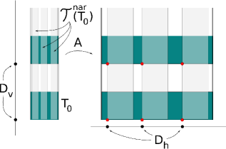
Figure 1. The tubes in $\mathcal{T}^{nar}(T_{0})$ and their images under $A$.

4.5. Absolute continuity with respect to a product measure

We now consider the following discrete measures:

$$\mu_{h}:=\frac{1}{|D_{h}|}\sum_{x\in D_{h}}\delta_{x}\quad\text{and}\quad\mu_{v}:=\frac{1}{|D_{v}|}\sum_{x\in D_{v}}\delta_{x}.$$ (4.33)

We also write $w_{x}:=|D_{h}|^{-1}$ and $w^{y}:=|D_{v}|^{-1}$, so that the product measure $\mu_{h}\times\mu_{v}$ on $D_{h}\times D_{v}$ can be written in the form

$$\mu_{h}\times\mu_{v}=\sum_{(x,y)\in D_{h}\times D_{v}}w_{x}w^{y}\cdot\delta_{(x,y)}.$$

We record that, by (4.27) and (4.31)-(4.32), we have

$$w_{x}w^{y}\approx\Delta^{dp+O_{N}(1)\alpha}.$$ (4.34)

Here, and in the sequel, the notation $O_{N}(1)$ refers to a constant with absolute value $\sim_{N}1$. For example, in the case (4.34) one could explicitly estimate that

$$w_{x}w^{y}\stackrel{{\scriptstyle\eqref{form51}\&\eqref{form61}}}{{\approx}}\Delta^{p(d-t_{th})+p(2t_{nar}-t_{th})},$$

where

$$\Delta^{dp+7\alpha p/q_{\text{spec}}}=\Delta^{p[d-s(e_{1})]+ps(e_{1})+7\alpha p/q_{\text{spec}}}\leq\Delta^{p(d-t_{th})+p(2t_{nar}-t_{th})}\leq\Delta^{dp-7\alpha p/q_{\text{spec}}},$$

and $q_{\text{spec}}=2^{-2N}$. Trying to track the constants in this fashion would soon become exceedingly cumbersome.

It may appear that the measure $\mu_{h}\times\mu_{v}$ has nothing to do with the "original" measure $\nu$ – or even its push-forward $A(\nu)$ – but in fact it does, and this is the next point of investigation. Roughly speaking, we wish to argue that the subset

$$A(T_{0}\cap G_{p}\cap K_{e}\cap K_{e_{1}})$$

has large $(\mu_{h}\times\mu_{v})$-measure, at least after it has been appropriately discretised to $D_{h}\times D_{v}$. Recall that $T_{0}\cap G_{p}\cap K_{e}\cap K_{e_{1}}$ readily has large $\nu$-measure by (4.25), so we roughly face the problem of showing that $A(\nu)\ll\mu_{h}\times\mu_{v}$ quantitatively.

We tackle the problem by defining another discrete measure on $D_{h}\times D_{v}$ which a priori more faithfully represents $A(\nu)$ than $\mu_{h}\times\mu_{v}$. Consider a point $(x,y)\in D_{h}\times D_{v}$. Then, recalling (4.26) and (4.30), we have

$$x=l(\pi_{1}(A(T)))\quad\text{and}\quad y=l(\pi_{2}(R))$$

for some $T\in\mathcal{T}^{nar}(T_{0})$ and some $R\in\mathcal{G}_{T_{0}}$. We define

$$w_{(x,y)}:=\frac{\nu([R\cap K_{e}\cap K_{e_{1}}\cap B(x_{R},\Delta^{p})]\cap T)}{(\Delta^{p})^{t_{th}}}$$ (4.35)

for these $R=R_{y}$ and $T=T_{x}$, where $x_{R}\in R\,\setminus\,\textbf{Bad}(q_{1},q_{2},e_{1})$ is the point selected at (4.24). Then, we set

$$\nu^{\prime}:=\sum_{(x,y)\in D_{h}\times D_{v}}w_{(x,y)}\cdot\delta_{(x,y)}.$$

How close is $\nu^{\prime}$ to the product measure $\mu_{h}\times\mu_{v}$? The latter gives weight $(|D_{h}||D_{v}|)^{-1}\approx\Delta^{dp+O_{N}(1)\alpha}$ to each pair $(x,y)\in D_{h}\times D_{v}$, so we would like to argue the weights $w_{(x,y)}$ "typically" have the same order of magnitude. This can be accomplished by one more "finding a bad ball" type argument, which we have already seen a few times.

Fix $y\in D_{v}$, and let $R\in\mathcal{G}_{T_{0}}$ be the square such that $y=l(\pi_{2}(R))$. Then,

$$\sum_{x\in D_{h}}w_{(x,y)} =\sum_{T\in\mathcal{T}^{nar}(T_{0})}\frac{\nu([R\cap K_{e}\cap K_{e_{1}}\cap B(x_{R},\Delta^{p})]\cap T)}{(\Delta^{p})^{t_{th}}}$$

$$\stackrel{{\scriptstyle\textup{(\hyperref@@ii[K1]{K1})}}}{{=}}\frac{\nu(R\cap K_{e}\cap K_{e_{1}}\cap B(x_{R},\Delta^{p}))}{(\Delta^{p})^{t_{th}}}\gtrapprox(\Delta^{p})^{d-t_{th}},$$ (4.36)

using first that the tubes $T\in\mathcal{T}^{nar}(T_{0})$ cover $K_{e_{1}}\cap R\subset K_{e_{1}}\cap T_{0}$ by (K1), and then recalling (4.24). Now, using the pigeonhole principle, we find a "typical" value of the weights in $w_{(x,y)}$, $x\in D_{h}$. In other words, first inferring the trivial upper bound

$$w_{(x,y)}\leq\frac{\nu(R)}{(\Delta^{p})^{t_{th}}}\leq(\Delta^{p})^{d-t_{th}},$$

from the Frostman condition for $\nu$, we find $\eta\in[0,d-t_{th}]$ and a further subset $D^{y}_{h}\subset D_{h}$ with the properties that

$$\sum_{x\in D_{h}^{y}}w_{(x,y)}\approx\sum_{x\in D_{h}}w_{(x,y)}\gtrapprox(\Delta^{p})^{d-t_{th}}\quad\text{and}\quad\Delta^{p\eta}\leq w_{(x,y)}\leq 2\Delta^{p\eta}\text{ for all }x\in D_{h}^{y}.$$ (4.37)

Here the number $\Delta^{p\eta}$ should be interpreted as the "typical value" of the constants $w_{(x,y)}$, $x\in D_{h}$, written as a power of $\Delta$ for clarity. Next, using once more the Frostman estimate for $\nu$, we infer that

$$|D_{h}^{y}|\cdot\Delta^{p\eta}\leq\sum_{x\in D_{h}}w_{(x,y)}\leq\sum_{T\in\mathcal{T}^{nar}(T_{0})}\frac{\nu(R\cap T)}{(\Delta^{p})^{t_{th}}}\leq(\Delta^{p})^{d-t_{th}},$$

whence

$$|D_{h}^{y}|\lesssim(\Delta^{p})^{d-t_{th}-\eta}.$$ (4.38)

Now, we claim that

$$\eta\geq d-\frac{4\alpha}{q_{\text{spec}}}.$$ (4.39)

Assume to the contrary: $\eta<d-4\alpha/q_{\text{spec}}$. Recalling from (4.27) (or (K1)) that $|t_{th}-s(e_{1})|\leq 2\alpha/q_{\text{spec}}$, and that $|s(e_{1})-s|<\alpha$, we see that

$$\eta+t_{th}-d<s(e_{1})-\frac{2\alpha}{q_{\text{spec}}}<s-2\alpha.$$ (4.40)

Now, let $\mathcal{T}_{y}$ be the collection of tubes in $\mathcal{T}^{nar}(T_{0})$ corresdponding to the points in $D_{h}^{y}$. More precisely, recall that every $x\in D_{h}^{y}\subset D_{h}$ has the form $x=l(\pi_{1}(A(T)))$ for some $T\in\mathcal{T}^{nar}(T_{0})$, and we denote the tubes of $\mathcal{T}^{nar}(T_{0})$ so obtained by $\mathcal{T}_{y}$. With this notation,

$$\sum_{T\in\mathcal{T}_{y}}\nu(T\cap B(x_{R},\Delta^{p})) \geq(\Delta^{p})^{t_{th}}\sum_{T\in\mathcal{T}_{y}}\frac{\nu([R\cap K_{e}\cap K_{e_{1}}\cap B(x_{R},\Delta^{p})]\cap T)}{(\Delta^{p})^{t_{th}}}$$

$$=(\Delta^{p})^{t_{th}}\sum_{x\in D_{h}^{y}}w_{(x,y)}\stackrel{{\scriptstyle\eqref{form59}}}{{\approx}}(\Delta^{p})^{t_{th}}\sum_{x\in D_{h}}w_{(x,y)}\gtrapprox\Delta^{dp},$$ (4.41)

recalling (4.36) in the last estimate. In other words, the collection $\mathcal{T}_{y}$ of $(\Delta^{q},e_{1})$-tubes of cardinality

$$|\mathcal{T}_{y}|=|D_{h}^{y}|\stackrel{{\scriptstyle\eqref{form57}\&\eqref{form104}}}{{\lesssim}}(\Delta^{p})^{-s+2\alpha}\stackrel{{\scriptstyle q=2p}}{{=}}(\Delta^{q-p})^{-s+2\alpha}$$

covers a set of $\nu$-measure $\gtrapprox\Delta^{pd}$ inside the ball $B(x_{R},\Delta^{p})=:B$. Consequently, a set of $\nu^{B}$-measure $\gtrapprox 1$ can be covered by a family $\mathcal{T}_{n+1}(e_{1})$ of $(\Delta^{q-p},e_{1})$-tubes of cardinality $|\mathcal{T}_{n+1}(e_{1})|\lesssim(\Delta^{q-p})^{-s+2\alpha}$. Now we may repeat an argument we have already seen many times (for example right after (3.55)): assuming that $f$ is rapidly increasing enough – depending on the implicit constants in the lower bound on line (4.41) – and using Lemma 3.12, we infer that $B$ is an $e_{1}$-bad ball relative to the scale $\Delta^{q}$. In particular $x_{R}\in\textbf{Bad}(p,q,e_{1})$, contrary to the choice of $x_{R}$ above (4.24). This contradiction establishes (4.39).

The upshot is that for any $y\in D_{v}$ fixed, there exists a subset $D_{h}^{y}\subset D_{h}$ such that (4.37) holds, and

$$w_{(x,y)}\sim\Delta^{p\eta}\leq(\Delta^{p})^{d-4\alpha/q_{\text{spec}}}\lessapprox\Delta^{-C_{N}\alpha}w_{x}w^{y},$$

recalling (4.34) in the final estimate; here $C_{N}\geq 1$ is a constant depending only on $N$. We write

$$G:=\bigcup_{y\in D_{v}}D_{h}^{y},$$

and then consider the restriction of $\nu^{\prime}$ to $G$:

$$\nu_{G}:=\sum_{(x,y)\in G}w_{(x,y)}\cdot\delta_{(x,y)}.$$

Then $\nu_{G}\ll\mu_{h}\times\mu_{v}$ with density

$$\frac{d\nu_{G}}{d(\mu_{h}\times\mu_{v})}\lessapprox\Delta^{-C_{N}\alpha},$$ (4.42)

and

$$\nu_{G}(D_{h}\times D_{v})=\sum_{y\in D_{v}}\sum_{x\in D_{h}^{y}}w_{(x,y)}\stackrel{{\scriptstyle\eqref{form59}}}{{\gtrapprox}}|D_{v}|\cdot(\Delta^{p})^{d-t_{th}}\stackrel{{\scriptstyle\eqref{form51}}}{{\gtrapprox}}1.$$ (4.43)

From (4.42)-(4.43), we finally infer that

$$(\mu_{h}\times\mu_{v})(\operatorname{spt}\nu_{G})\gtrapprox\Delta^{C_{N}\alpha}.$$ (4.44)

4.6. Projecting the measures $\mu_{h}\times\mu_{v}$ and $\nu_{G}$

Recall that we are in the process of proving Proposition 4.17: for a fixed vector $e\in S_{1}\subset J_{1}$, we are trying to show that

$$|e-(1,0)|=|e-e_{1}|\leq\Delta^{q-\epsilon_{1}},$$ (4.45)

where $\epsilon_{1}=2^{-N}$ according to the choice made in (4.13). This will be true if $\alpha=\alpha(N)>0$ and $\tau=\tau(\alpha,N)>0$ are chosen sufficiently small. We now make a counter assumption:

$$\Delta^{q-\epsilon_{1}}<|e-e_{1}|\lesssim\Delta^{p},$$ (4.46)

where the upper bound follows from $e\in J_{1}$.

So far, the role of the vector $e$ has been passive, but now we concentrate on it. Recall from (K1) that the set $K_{e}$ is contained in the union of the $(\Delta^{q},e)$-tubes in the collection $\mathcal{T}^{nar}(e)$. We want to say something a little sharper concerning the intersection $K_{e}\cap T_{0}$: because $|e-e_{1}|\leq\operatorname{diam}(S_{1})\lesssim\Delta^{p}$, and $T_{0}\in\mathcal{T}^{th}=\mathcal{T}^{th}(e_{1})$ is a tube of width $\Delta^{p}$, we first note that

$$|\{T\in\mathcal{T}^{th}(e):T\cap T_{0}\neq\emptyset\}|\lesssim 1.$$

The tube $T_{0}$ and one of the $\lesssim 1$ tubes in $T\in\mathcal{T}^{th}(e)$ with $T\cap T_{0}\neq\emptyset$ are shown in Figure 2. So, $K_{e}\cap T_{0}$ is covered by the union of the tubes in $\mathcal{T}^{nar}(e)$ contained in one of $\lesssim 1$ tubes in $\mathcal{T}^{th}(e)$. We denote this collection by $\mathcal{T}^{nar}(e,T_{0})$. Recalling (K1), and that $q=2p$, we then infer that

$$|\mathcal{T}^{nar}(e,T_{0})|\lessapprox\Delta^{-t_{nar}(e)q+t_{th}(e)p}=\Delta^{-p(2t_{nar}(e)-t_{th}(e))}=(\Delta^{p})^{-s+O_{N}(1)\alpha},$$ (4.47)

since (repeating (4.32)), we have

$$|(2t_{nar}(e)-t_{th}(e))-s(e)|\leq\frac{6\alpha}{q_{\text{spec}}}.$$

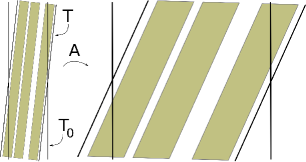
Figure 2. Some tubes in $\mathcal{T}^{nar}(e,T_{0})$ and their images under the map $A$.

We next claim that

$$\operatorname{spt}\nu_{G}=\{(x,y)\in D_{h}\times D_{v}:w_{(x,y)}>0\}\subset\bigcup_{T\in\mathcal{T}^{nar}(e,T_{0})}A(T)(C\Delta^{p}),$$ (4.48)

where $C\geq 1$ is an absolute constant, and $A(T)(C\Delta^{p})$ means the $C\Delta^{p}$-neighbourhood of $A(T)$. The sets $A(T)(C\Delta^{p})$ are not exactly tubes in the strict sense of this paper, but they are each contained in an ordinary $(C\Delta^{p},e^{\prime})$-tube, where

$$|e_{1}-e^{\prime}|\sim\Delta^{-p}|e_{1}-e|.$$ (4.49)

By an ordinary $(w,e^{\prime})$-tube, we mean a set of the form $\pi_{e^{\prime}}^{-1}(I)$, where $I\subset\mathbb{R}$ and $\ell(I)=w$. For a proof of these claims on the geometry of $A(T)$, see Figure 3.

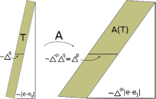
Figure 3. The geometry of the images $A(T)$ for $T\in\mathcal{T}^{nar}(e,T_{0})$.

In combination with (4.47), (4.48) will therefore have the following corollary:

Proposition 4.50.

$N(\pi_{e^{\prime}}(\operatorname{spt}\nu_{G}),\Delta^{p})\lessapprox(\Delta^{p})^{-s-C_{N}\alpha}$, where $e^{\prime}\in S^{1}$ satisfies (4.49).

We then prove (4.48). Pick $(x,y)\in D_{h}\times D_{v}$ with $w_{(x,y)}>0$. Let $R\in\mathcal{G}_{T_{0}}$ and $T_{e_{1}}\in\mathcal{T}^{nar}(T_{0})$ be such that

$$y=l(\pi_{2}(R))\quad\text{and}\quad x=l(\pi_{2}(A(T_{e_{1}}))).$$

Then $(x_{0},y_{0}):=A^{-1}(x,y)=(\Delta^{p}x,y)\in R\cap T_{e_{1}}$. Moreover, recalling the definition (4.35),

$$w_{(x,y)}>0\quad\Longrightarrow\quad\nu(R\cap K_{e}\cap T_{e_{1}})>0,$$

so in particular there exists a tube $T_{e}\in\mathcal{T}^{nar}(e,T_{0})$ such that $\nu(R\cap T_{e_{1}}\cap T_{e})>0$. Now, pick a point $(x^{\prime},y^{\prime})\in R\cap T_{e_{1}}\cap T_{e}$, and note that

$$|x_{0}-x^{\prime}|\leq\Delta^{q}\quad\text{and}\quad|y_{0}-y^{\prime}|\leq\Delta^{p}.$$

It follows that

$$|(x,y)-A(x^{\prime},y^{\prime})|=|A(x_{0},y_{0})-A(x^{\prime},y^{\prime})|=|(\Delta^{-p}(x_{0}-x^{\prime}),y_{0}-y^{\prime})|\lesssim\Delta^{p}.$$

Because $A(x^{\prime},y^{\prime})\in A(T_{e})$, we infer that also $(x,y)\in A(T_{e})(C\Delta^{p})$ for some absolute constant $C\geq 1$. This proves (4.48).

We next aim to use Proposition 4.50 to derive a contradiction from the lower bound in (4.46). First, from (4.49) and (4.46), we infer that

$$|e^{\prime}-e_{1}|\sim\Delta^{-p}|e-e_{1}|\geq\Delta^{q-p-\epsilon_{1}}=\Delta^{p-\epsilon_{1}}\quad\text{and}\quad|e^{\prime}-e_{1}|\lesssim 1.$$

Now, fix $\theta\in\mathbb{R}$ such that $(1,\theta)\|e^{\prime}$. Then, $\Delta^{p-\epsilon_{1}}\lesssim|\theta|\lesssim 1$, and for slight notational convenience, we work under the assumption that

$$\theta\gtrsim\Delta^{p-\epsilon_{1}}.$$ (4.51)

We now wish to compute some $L^{2}$-norms of the measures $\mu_{h}$ and $\mu_{h}\ast\theta\mu_{v}$, where $\theta\mu_{v}$ refers to the push-forward of $\mu_{v}$ under the map $x\mapsto\theta x$. These are discrete measures, so their $L^{2}$-norm, literally speaking, is infinity. However, we can obtain useful information by mollifying the measures first at scale $\Delta^{p}$. To this end, let $\psi:=\tfrac{1}{2}\chi_{[-1,1]}$, and for $\rho>0$, define $\psi_{\rho}(x):=\rho^{-1}\psi(x/\rho)=\tfrac{1}{2\rho}\chi_{[-\rho,\rho]}$. Then, recalling that $\mu_{h}$ was a (normalised) sum of Dirac measures supported on the $\Delta^{p}$-separated set $D_{h}$, see (4.33), it is easy to see that

$$\|\mu_{h}\ast\psi_{\Delta^{p}}\|_{L^{2}}\sim\left(\frac{1}{\Delta^{p}|D_{h}|}\right)^{1/2}\approx(\Delta^{p})^{(s-1)/2+O_{N}(1)\alpha},$$ (4.52)

recalling from (4.31)-(4.32) that $|D_{h}|\approx(\Delta^{p})^{-s+O_{N}(1)\alpha}$ in the last estimate. Next, we investigate the $L^{2}$-norm of the convolution $\mu_{h}\ast\theta\mu_{v}$. From the choice of $\theta$, namely $(1,\theta)\|e^{\prime}$, one can easily verify that

$$\mu_{h}\ast\theta\mu_{v}=|(1,\theta)|_{\sharp}[\pi_{e^{\prime}}(\mu_{h}\times\mu_{v})],$$

so (using also $|(1,\theta)|\sim 1$), we infer that

$$\|(\mu_{h}\ast\theta\mu_{v})\ast\psi_{\Delta^{p}}\|_{L^{2}}\sim\|\pi_{e^{\prime}}(\mu_{h}\times\mu_{v})\ast\psi_{\Delta^{p}}\|_{L^{2}}.$$ (4.53)

To estimate the quantity on the right hand side, we start by noting that the support of the measure

$$\pi_{e^{\prime}}[(\mu_{h}\times\mu_{v})|_{\operatorname{spt}\nu_{G}}]\ast\psi_{\Delta^{p}}$$

is contained in the $2\Delta^{p}$-neighbourhood of the set $\pi_{e^{\prime}}(\operatorname{spt}\nu_{G})$, and hence, by Proposition 4.50, has Lebesgue measure no larger than $\lessapprox(\Delta^{p})^{1-s-C_{N}\alpha}$. Consequently, using (4.44) (plus the fact that neither push-forward nor convolution with $\psi_{\Delta^{p}}$ affects total variation), and then the Cauchy-Schwarz inequality, we obtain

$$\Delta^{C_{N}\alpha}\stackrel{{\scriptstyle\eqref{form67}}}{{\lessapprox}}\|\pi_{e^{\prime}}[(\mu_{h}\times\mu_{v})|_{\operatorname{spt}\nu_{G}}]\ast\psi_{\Delta^{p}}\|_{L^{1}}\lessapprox\left((\Delta^{p})^{1-s-C_{N}\alpha}\right)^{1/2}\|\pi_{e^{\prime}}(\mu_{h}\times\mu_{v})\ast\psi_{\Delta^{p}}\|_{L^{2}}.$$

Combining this estimate with (4.52)-(4.53), we have now established that

$$\|(\mu_{h}\ast\theta\mu_{v})\ast\psi_{\Delta^{p}}\|_{L^{2}}\gtrapprox\Delta^{C_{N}\alpha}\|\mu_{h}\ast\psi_{\Delta^{p}}\|_{L^{2}}.$$ (4.54)

The estimate (4.54) will soon place us in a position to apply Shmerkin’s inverse theorem, [24, Theorem 2.1], the relevant parts of which are also stated as Theorem 4.63 below. Before doing so, we make some remarks. First, note from (4.29)-(4.30) that

$$\Delta^{p}\cdot[\operatorname{spt}\mu_{h}]=\Delta^{p}\cdot D_{h}=\{l(\pi_{1}(T))):T\in\mathcal{T}^{nar}(T_{0})\}.$$

In particular, since $\nu(K_{e_{1}}\cap T)>0$ for all $T\in\mathcal{T}^{nar}(T_{0})$ by (K1), we have

$$\Delta^{p}\cdot[\operatorname{spt}\mu_{h}]\subset\pi_{1}(T_{0})\cap[\pi_{1}(K_{e_{1}})](\Delta^{q}).$$ (4.55)

Now, we apply the facts that $e_{1}\in S_{1}\subset\operatorname{spt}\sigma$ and $\nu=\mu^{B(x_{0},R_{0})}$, which imply that (4.4) holds for $e_{1}$, and for $\operatorname{spt}\nu$ in place of $K$:

$$N(\pi_{e_{1}}(\operatorname{spt}\nu\cap B_{0})\cap B(x,R),r)\leq C_{E}\left(\frac{R}{r}\right)^{D}$$

for all $x\in\mathbb{R}$ and $0<r<R<\infty$. In particular, the estimate above holds for all $B(x,R)\subset\pi_{1}(T_{0})$ and all $\Delta^{q}<r<R\leq\Delta^{p}$. It follows from this, $K_{e_{1}}\subset\operatorname{spt}\nu\cap B_{0}$, and (4.55) that

$$N([\operatorname{spt}\mu_{h}]\cap B(x,R),r)\lesssim C_{E}\left(\frac{R}{r}\right)^{D},\qquad x\in\mathbb{R},\>\Delta^{p}\leq r<R\leq 1.$$ (4.56)

Here $0<D<\min\{d,1\}$, so (4.56) means that the support of $\mu_{h}$ is porous on all scales between $\Delta^{p}$ and $1$. This is good news in view of applying Shmerkin’s inverse theorem, but we also need to know something about the measure $\theta\mu_{v}$, namely that it cannot be concentrated on a very small number of $\Delta^{p}$-intervals.

4.7. Non-concentration of $\theta\mu_{v}$

The goal in this section is to show that

$$(\theta\mu_{v})(I)\lessapprox\Delta^{q_{\text{spec}}(d-s)-C_{N}\alpha}$$ (4.57)

for any interval $I\subset\mathbb{R}$ of length $\ell(I)=\Delta^{p}$. Here we need to know that

$$q_{\text{spec}}=2^{-2N}<2^{-N}=\epsilon_{1},$$

recall the choices (4.5) and (4.13). Then, recalling from (4.12) that $s<(d+D)/2$, taking $\alpha,\Delta>0$ sufficiently small in terms of $N$, we will find that

$$(\theta\mu_{v})(I)\leq\Delta^{q_{\text{spec}}(d-D)/3}\qquad\text{ for all }I\subset\mathbb{R}\text{ with }\ell(I)=\Delta^{p}.$$ (4.58)

Recall from (4.51) that $\theta\gtrsim\Delta^{p-\epsilon_{1}}$, so (4.57) will follow once we manage to prove that

$$\mu_{v}(I)\lessapprox\Delta^{q_{\text{spec}}(d-s(e_{1}))-4\alpha/q_{\text{spec}}}$$ (4.59)

for all intervals $I\subset\mathbb{R}$ of length $\Delta^{\epsilon_{1}}$. Furthermore, since $q_{\text{spec}}<\epsilon_{1}$, it suffices to verify (4.59) for all dyadic intervals of length $\Delta^{q_{\text{spec}}}$. We fix one such interval $I$. Recall from (4.33) the definition of $\mu_{v}$:

$$\mu_{v}=\frac{1}{|D_{v}|}\sum_{x\in D_{v}}\delta_{x}\stackrel{{\scriptstyle\eqref{form51}}}{{\approx}}(\Delta^{p})^{d-t_{th}}\sum_{x\in D_{v}}\delta_{x}.$$

For each $x\in D_{v}\cap I$, let $R\in\mathcal{G}_{T_{0}}$ be the heavy square such that $R\subset T_{0}$ and $x=l(\pi_{2}(R))$; then, since $I$ is a dyadic interval, we have $\pi_{2}(R)\subset I$, and hence $R\subset\pi_{2}^{-1}(I)$. It follows that

$$|D_{v}\cap I|\leq\operatorname{card}\{R\in\mathcal{G}_{T_{0}}:R\subset\pi_{2}^{-1}(I)\}.$$

Next, by the definition of heavy squares in (4.21), we recall that

$$\nu(R\cap K_{e_{1}})\gtrapprox\Delta^{dp},$$

and consequently

$$\mu_{v}(I)\approx(\Delta^{p})^{d-t_{th}}\cdot|D_{v}\cap I|\lessapprox(\Delta^{p})^{-t_{th}}\nu(T_{0}\cap K_{e_{1}}\cap\pi_{2}^{-1}(I)).$$ (4.60)

We recall from (K1) that the set $T_{0}\cap K_{e_{1}}$ is covered by the $(\Delta,e_{1})$-tubes in $\mathcal{T}^{0}(T_{0})=\{T\in\mathcal{T}^{0}:T\subset T_{0}\}$, and consequently

$$\nu(T_{0}\cap K_{e_{1}}\cap\pi_{2}^{-1}(I))=\sum_{T\in\mathcal{T}^{0}(T_{0})}\nu(T\cap K_{e_{1}}\cap\pi_{2}^{-1}(I)).$$ (4.61)

Further, by iterating the branching estimate $|\mathcal{T}^{k-1}(T^{k})|\approx|\mathcal{T}^{k-1}|/|\mathcal{T}^{k}|$ in (K1) in the same manner as we did in (3.50), we have

$$|\mathcal{T}^{0}(T_{0})|\approx\frac{|\mathcal{T}^{0}|}{|\mathcal{T}^{th}|}\approx\Delta^{-s(e_{1})+pt_{th}},$$ (4.62)

recalling also the choice of the number $t_{th}$ from under (4.19). We now fix a tube $T\in\mathcal{T}^{0}(T_{0})$, and note that the intersection $T\cap\pi_{2}^{-1}(I)$ can be covered by $\lesssim 1$ balls of radius $\Delta^{q_{\text{spec}}}$. Now, we finally use the non-concentration estimate from (K2), which we repeat here for convenience:

$$\frac{\nu([K_{e_{1}}\cap T]\cap B(x,\Delta^{q_{\text{spec}}}))}{\nu(T)}\lesssim(\Delta^{q_{\text{spec}}})^{d-s(e)-4\alpha/q_{\text{spec}}},\qquad x\in\mathbb{R}^{2},\>T\in\mathcal{T}^{0}.$$

Recalling (this is also stated in (K2)) that $\nu(T)\approx\Delta^{s(e_{1})}$ for $T\in\mathcal{T}^{0}$, we may combine the estimate above with (4.60)-(4.62) to obtain

$$\mu_{v}(I)\lessapprox(\Delta^{p})^{-t_{th}}\cdot|\mathcal{T}^{0}(T_{0})|\cdot\Delta^{s(e_{1})+q_{\text{spec}}(d-s(e_{1}))-4\alpha/q_{\text{spec}}}\lessapprox\Delta^{q_{\text{spec}}(d-s(e_{1}))-4\alpha/q_{\text{spec}}},$$

which is precisely (4.59).

4.8. Applying Shmerkin’s inverse theorem

Now, we have gathered all the pieces to apply Shmerkin’s inverse thereorem [24, Theorem 2.1], whose statement (in reduced form) we also include right here for the reader’s convenience. We explain the notions appearing in the theorem afterwards.

Theorem 4.63 (Shmerkin).

Given $\beta>0$ and $m_{0}\in\mathbb{N}$, there are $\kappa>0$ and $m\geq m_{0}$ such that the following holds for all large enough $\ell$. Let $\Delta=2^{-\ell m}$, and let $\mu,\nu$ be $\Delta$-measures such that

$$\|\mu\ast\nu\|_{L^{2},\textup{Sh}}\geq\Delta^{\kappa}\|\mu\|_{L^{2},\textup{Sh}}.$$ (4.64)

Then, there exist sets $A\subset\operatorname{spt}\mu$ and $B\subset\operatorname{spt}\nu$ such that

• there is a sequence $(R_{s}^{\mu})_{s=0}^{\ell}\subset\{1,\ldots,2^{m}\}^{\ell+1}$, such that

  $$N(A\cap I,2^{-(s+1)m})=R_{s}^{\mu}$$

  for all dyadic intervals $I$ of length $2^{-ms}$ intersecting $A$,

• there is a sequence $(R_{s}^{\nu})_{s=0}^{\ell}\subset\{1,\ldots,2^{m}\}^{\ell+1}$, such that

  $$N(B\cap I,2^{-(s+1)m})=R_{s}^{\nu}$$

  for all dyadic intervals $I$ of length $2^{-ms}$ intersecting $B$.

For each $s\in\{0,\ldots,\ell\}$, either $R_{s}^{\nu}=1$ or $R_{s}^{\mu}\geq 2^{(1-\beta)m}$, and the set $\mathcal{S}=\{s:R_{s}^{\mu}\geq 2^{(1-\beta)m}\}$ satisfies

$$m|\mathcal{S}|\geq\log\|\nu\|_{L^{2},\textup{Sh}}^{-2}+\beta\log_{2}\Delta.$$ (4.65)

Now, we explain the concepts appearing above. First, for $\Delta\in 2^{-\mathbb{N}}$, a $\Delta$-measure is any probability measure in $\mathcal{M}(\Delta\cdot\mathbb{Z}\cap[-1,1))$. In our case, we will actually be concerned with $\Delta^{p}$-measures, such as $\mu_{h}$. For a $\Delta$-measure $\mu\in\mathcal{M}(\Delta\cdot\mathbb{Z}\cap[-1,1))$, Shmerkin defines the (non-standard) $L^{2}$-norm

$$\|\mu\|_{L^{2},\textup{Sh}}^{2}:=\sum_{x\in\Delta\cdot\mathbb{Z}\cap[-1,1)}\mu(\{x\})^{2}.$$

It is easy to see that

$$\|\mu\|_{L^{2},\textup{Sh}}^{2}\sim\Delta\cdot\|\mu\ast\psi_{\Delta}\|_{L^{2}}^{2},\qquad\mu\in\mathcal{M}(\Delta\cdot\mathbb{Z}\cap[-1,1)).$$ (4.66)

Of the measures we are interested in presently, $\mu_{h}$ is already a $\Delta^{p}$-measure, but $\theta\mu_{v}$ is not. However, we can associate to $\theta\mu_{v}$ a $\Delta^{p}$-measure in the following canonical way:

$$(\theta\mu_{v})^{\prime}:=\sum_{x\in D_{p}}(\theta\mu_{v})([x,x+\Delta^{p}))\cdot\delta_{x}.$$

Then, it follows from (4.58) that $(\theta\mu_{v})^{\prime}(\{x\})\leq\Delta^{\eta p}$ for $\eta=q_{\textup{spec}}(d-D)/3$, and consequently (noting that $(\theta\mu_{v})^{\prime}$ is a probability measure)

$$\|(\theta\mu_{v})^{\prime}\|_{L^{2},\textup{Sh}}^{2}=\sum_{2^{-j}\leq\Delta^{\eta p}}\mathop{\sum_{x\in D_{p}}}_{2^{-j-1}<(\theta\mu_{v})^{\prime}(\{x\})\leq 2^{-j}}(\theta\mu_{v})^{\prime}(\{x\})^{2}\leq 2\Delta^{\eta p}.$$

As a technical corollary, noting also that $\Delta^{-p}\geq|D_{p}|/2$, we record that

$$\log\|(\theta\mu_{v})^{\prime}\|_{L^{2},\textup{Sh}}^{-2}\geq\eta\log\Delta^{-p}-2=\eta\log|D_{p}|-3.$$ (4.67)

We further record the following consequence of (4.54) and (4.66):

$$\|\mu_{h}\ast(\theta\mu_{v})^{\prime}\|_{L^{2},\textup{Sh}}\gtrapprox\Delta^{C_{N}\alpha}\|\mu_{h}\|_{L^{2},\textup{Sh}},$$ (4.68)

Then, we apply Shmerkin’s inverse theorem to the measures $\mu_{h}$ and $(\theta\mu_{v})^{\prime}$, for any

$$0<\beta<\min\{\eta/2,(1-D)\}=\min\{q_{\text{spec}}(d-D)/6,(1-D)\},$$

and for some large $m_{0}\in\mathbb{N}$ to be prescribed in a moment, depending only on $1-D$ and the constant $C_{E}$ in (4.56). The inverse theorem then produces the constants

$$m=m(\beta,m_{0})\geq m_{0}\quad\text{and}\quad\kappa=\kappa(\beta,m_{0})>0.$$

Note that the choice of $\beta$ can be made depending only on $q_{\text{spec}}=2^{-2N},d-D$ and $1-D$, and $N$ further only depends on $\epsilon_{0}$ (recall the choice made in (4.6)). So, $\kappa$ only depends on $\epsilon_{0}$, $d-D$, $1-D$ and the constant $C_{E}$ in (4.56). We may assume that $\Delta^{p}$ has the form

$$\Delta^{p}=2^{-\ell m}\quad\text{for some}\quad\ell\in\mathbb{N}.$$

This can be achieved by adding one more requirement for $\delta>0$ at the start of Section 3.3.1 (instead of asking that $\delta^{g^{-n}}\in 2^{-\mathbb{N}}$ for all $n\lesssim 1/\alpha$, we rather require that $\delta^{g^{-n}}\in 2^{-m\mathbb{N}}$ for the $m$ above, which only depends on $\epsilon_{0},d-D,1-D$, and the constant $C_{E}$ in (4.56)).

Then, we pick $\alpha$ so small that $C_{N}\alpha<\kappa$ in (4.68). Then, (4.68) implies – for $\Delta>0$ small enough, and finally picking $\tau>0$ small enough depending on $\alpha,N$ – that the main hypothesis (4.64) of Theorem 4.63 is valid. It follows from the theorem that (4.65) is valid. Then, combining (4.65) and (4.67), we find that

$$m|\mathcal{S}|\geq\log\|(\theta\mu_{v})^{\prime}\|_{L^{2},\textup{Sh}}^{-2}+\beta\log\Delta^{p}\geq(\eta-\beta)\log|D_{p}|-3\geq\tfrac{\eta}{2}\log|D_{p}|-3.$$

If $\Delta^{p}$ is small enough, and hence $|D_{p}|$ is large enough, the inequality above implies that $m|\mathcal{S}|>0$, and hence $\mathcal{S}\neq\emptyset$. (Choosing $\Delta^{p}$ small enough depending on $\eta$ is legitimate: recall that $\eta=q_{\mathrm{spec}}(d-D)/3$, and then from Section 4.2 that $q_{\mathrm{spec}}=2^{-2N}$ and $p\in[2^{-N+2},1]$, where $N$ only depends on $D-d$ and $\epsilon_{0}$. Also, recall from (3.22) and (3.27) that $\Delta=\delta_{n}=\delta^{\kappa}$, where $\kappa>0$ is a constant depending only on $\alpha,Q$, and $\delta>0$ is an "initial scale", chosen as early as in Section 3.3.1. This scale was allowed to depend on all the parameters $\alpha,d,D,\epsilon_{0},Q$. Therefore, we can arrange $\log|D_{p}|\gg 2/\eta$ by choosing $\delta>0$ initially small enough, depending only on $\alpha,d,D,\epsilon_{0},Q$.) Recalling Theorem 4.63(A), it follows that there exists $s\in\mathcal{S}\subset\{0,\ldots,\ell\}$ such that

$$N([\operatorname{spt}\mu_{h}]\cap I,2^{-(s+1)m})\geq R_{s}^{\mu}\geq 2^{(1-\beta)m}$$ (4.69)

for some dyadic interval $I\subset\mathbb{R}$ of length $\ell(I)=2^{-ms}\in[\Delta^{p},1]$. On the other hand, by (4.56) applied with $R=2^{-ms}$ and $r=2^{-(s+1)m}$, we find that

$$N([\operatorname{spt}\mu_{h}]\cap I,2^{-(s+1)m})\lesssim C_{E}\left(\frac{2^{-ms}}{2^{-(s+1)m}}\right)^{D}=C_{E}\cdot 2^{mD}.$$ (4.70)

Finally, since $\beta<1-D$, we see that the inequalities (4.69)-(4.70) are incompatible if $m\geq m_{0}$ is sufficiently large (depending on $1-D$ and $C_{E}$, as promised). We have reached a contradiction, and proved (4.45), namely that $|e-e_{1}|\leq\Delta^{p-\epsilon_{1}}$, and hence Proposition 4.17. As explained after (4.18), this implies the existence of the arc $J_{2}\subset J_{1}$ satisfying (4.14).

4.9. Conclusion of the proof

We now complete the proof of Theorem 3.4 roughly in the way described in Section 4.2.1. We pick any initial arc $J_{1}\subset S^{1}$ of length $\ell(J_{1})\sim\Delta^{q_{2}}$ and $\sigma(J_{1})\gtrsim\Delta^{q_{2}}$. Then, we apply (4.14) repeatedly to find a sequence of arcs $J_{1}\supset J_{2}\supset\ldots\supset J_{N-1}$ with the properties that

• $\ell(J_{j})=\Delta^{q_{j+1}}$ for $1\leq j\leq N-1$, and

• $\sigma(J_{j+1})\gtrapprox\Delta^{\epsilon_{1}}\sigma(J_{j})$ for $1\leq j\leq N-2$.

In particular $J:=J_{N-1}$ is an arc of length $\Delta$ satisfying

$$\sigma(J)\gtrapprox\Delta^{N\epsilon_{1}}\sigma(J_{1})\gtrsim\Delta^{N\cdot 2^{-N}\cdot 2^{-N+2}}=\Delta^{(N+3)\cdot 2^{-N}}.$$

On the other hand, $\sigma(J)\leq C_{\sigma}\Delta^{\epsilon_{0}}$ by (4.3). Recalling from (4.6) that $10N\cdot 2^{-N}<\epsilon_{0}$, we have reached a contradiction, assuming that $\Delta,\tau>0$ are small enough. The proof of Theorem 3.4 is complete.

References

- [1] Balázs Bárány, Michael Hochman, and Ariel Rapaport. Hausdorff dimension of planar self-affine sets and measures. Invent. Math. (to appear), page arXiv:1712.07353.
- [2] J. Bourgain. On the Erdös-Volkmann and Katz-Tao ring conjectures. Geom. Funct. Anal., 13(2):334–365, 2003.
- [3] Jean Bourgain. The discretized sum-product and projection theorems. J. Anal. Math., 112:193–236, 2010.
- [4] Catherine Bruce and Xiong Jin. Projections of Gibbs measures on self-conformal sets. arXiv e-prints, page arXiv:1801.06468, January 2018.
- [5] K. J. Falconer and J. D. Howroyd. Projection theorems for box and packing dimensions. Math. Proc. Cambridge Philos. Soc., 119(2):287–295, 1996.
- [6] Katrin Fässler and Tuomas Orponen. On restricted families of projections in . Proc. Lond. Math. Soc. (3), 109(2):353–381, 2014.
- [7] Andrew Ferguson, Jonathan M. Fraser, and Tuomas Sahlsten. Scaling scenery of invariant measures. Adv. Math., 268:564–602, 2015.
- [8] Jonathan M. Fraser. Distance sets, orthogonal projections and passing to weak tangents. Israel J. Math., 226(2):851–875, 2018.
- [9] Jonathan M. Fraser and Antti Käenmäki. Attainable values for the Assouad dimension of projections. arXiv e-prints, page arXiv:1811.00951, November 2018.
- [10] Jonathan M. Fraser and Tuomas Orponen. The Assouad dimensions of projections of planar sets. Proc. Lond. Math. Soc. (3), 114(2):374–398, 2017.
- [11] Hillel Furstenberg. Ergodic fractal measures and dimension conservation. Ergodic Theory Dynam. Systems, 28(2):405–422, 2008.
- [12] Juha Heinonen. Lectures on analysis on metric spaces. Universitext. Springer-Verlag, New York, 2001.
- [13] Michael Hochman. Dynamics on fractals and fractal distributions. arXiv e-prints, page arXiv:1008.3731, August 2010.
- [14] Michael Hochman. On self-similar sets with overlaps and inverse theorems for entropy. Ann. of Math. (2), 180(2):773–822, 2014.
- [15] Maarit Järvenpää. On the upper Minkowski dimension, the packing dimension, and orthogonal projections. Ann. Acad. Sci. Fenn. Ser. A I Math. Dissertationes, (99):34, 1994.
- [16] Antti Käenmäki, Tuomo Ojala, and Eino Rossi. Rigidity of quasisymmetric mappings on self-affine carpets. Int. Math. Res. Not. IMRN, (12):3769–3799, 2018.
- [17] R. Kaufman and P. Mattila. Hausdorff dimension and exceptional sets of linear transformations. Ann. Acad. Sci. Fenn. Ser. A I Math., 1(2):387–392, 1975.
- [18] Robert Kaufman. On Hausdorff dimension of projections. Mathematika, 15:153–155, 1968.
- [19] John M. Mackay and Jeremy T. Tyson. Conformal dimension, volume 54 of University Lecture Series. American Mathematical Society, Providence, RI, 2010. Theory and application.
- [20] J. M. Marstrand. Some fundamental geometrical properties of plane sets of fractional dimensions. Proc. London Math. Soc. (3), 4:257–302, 1954.
- [21] Tuomas Orponen. An improved bound on the packing dimension of Furstenberg sets in the plane. J. Eur. Math. Soc. (to appear), page arXiv:1611.09762.
- [22] Tuomas Orponen. On the packing dimension and category of exceptional sets of orthogonal projections. Ann. Mat. Pura Appl. (4), 194(3):843–880, 2015.
- [23] Yuval Peres and Pablo Shmerkin. Resonance between Cantor sets. Ergodic Theory Dynam. Systems, 29(1):201–221, 2009.
- [24] Pablo Shmerkin. On Furstenberg’s intersection conjecture, self-similar measures, and the norms of convolutions. Ann. of Math. (to appear), page arXiv:1609.07802.