Chain-referral sampling on Stochastic Block Models
Abstract.
The discovery of the “hidden population”, whose size and membership are unknown, is made possible by assuming that its members are connected in a social network by their relationships. We explore these groups by a chain-referral sampling (CRS) method, where participants recommend the people they know. This leads to the study of a Markov chain on a random graph where vertices represent individuals and edges connecting any two nodes describe the relationships between corresponding people. We are interested in the study of CRS process on the stochastic block model (SBM), which extends the well-known Erdös-Rényi graphs to populations partitioned into communities. The SBM considered here is characterized by a number of vertices , a number of communities (blocks) , proportion of each community and a pattern for connection between blocks . In this paper, we give a precise description of the dynamic of CRS process in discrete time on an SBM. The difficulty lies in handling the heterogeneity of the graph. We prove that when the population’s size is large, the normalized stochastic process of the referral chain behaves like a deterministic curve which is the unique solution of a system of ODEs.
Key words and phrases:
chain-referral sampling, random graph, social network, stochastic block model, exploration process, large graph limit, respondent driven sampling1991 Mathematics Subject Classification:
05C80; 60J05; 60F17; 90B15; 92D30; 91D30Nous nous intéressons à l’étude de “populations cachées”, de taille inconnue, et dont on ne connaît pas les membres. La découverte d’une population cachée est rendue possible en supposant que ses individus sont connectés par un réseau social. Nous explorons ces groupes par une méthode de sondage par chaînage (“Chain referral sampling”, CRS), où les répondants recommandent leurs contacts. Ceci conduit à l’étude d’une chaîne de Markov sur un graphe aléatoire dont les sommets représentent les individus et dont les arêtes décrivent les relations entre les deux personnes qu’elles relient. Les personnes interrogées sont invitées à indiquer leurs partenaires et un certain nombre de coupons est remis à certaines de ces personnes. Le sondage par chaînage recherche les noeuds cachés dans la population en suivant au hasard les arêtes du réseau social sous-jacent, ce qui permet de tracer les individus échantillonnés. Nous étudions le processus CRS lorsque le réseau est un modèle à blocs stochastiques (“Stochastic Block Model”, SBM), qui est une extension du modèle d’Erdös-Rényi aux populations partitionnées en communautés. Le SBM considéré ici est caractérisé par un certain nombre de sommets (taille de la population), un certain nombre de communautés (blocs) , une distribution de blocs représentant la proportion de chaque communauté et une matrice permettant de définir les liens entre sommets appartenant à des blocs donnés . Dans cet article, nous donnons une description précise de la dynamique du processus CRS en temps discret sur un SBM. La difficulté réside dans la gestion de l’hétérogénéité du graphe. Dans notre modèle, le graphe et la marche aléatoire sont construits simultanément. Ensuite, nous étudions l’évolution de cette chaîne en considérant le processus normalisé sur l’échelle de temps . Nous démontrons que lorsque la taille de la population est grande, le processus aléatoire CRS normalisé se comporte comme une courbe déterministe qui est la solution unique d’un système d’ODE.
1. Introduction
In Sociology, some populations may be hidden because their members share common attributes that are illegal or stigmatized. These hidden groups may be hard to approach because these individuals try to conceal their identities due to legal authorities (e.g. drugs users) or because of the social pressure (e.g. men having sex with men). In such populations, all the information is unknown: there is no sampling frame such as lists of the members of the population or of the relationship between the latter. It causes many challenges for researchers to identify these groups. The discovery of the hidden populations is made possible by assuming that its members are connected by a social network. The population is described by a graph (network) where each individual is represented by a vertex and any interaction or relationship (e.g. friendship, partnership) between a couple of individuals is represented by an edge matching the corresponding vertices. Thanks to this important feature, we are allowed to investigate these populations by using a Chain-referral Sampling (CRS) technique, such as snowball sampling, targeting sampling, respondent driven sampling etc. (see the review of [25] or [16, 17, 18]). CRS consists in detecting hidden individuals in a population structured as a random graph, which is modeled by a stochastic process that we study here. The principle of CRS is that from a group of initially recruited individuals, we follow their connections in the social network to recruit the subsequent participants. The exploration proceeds from node to node along the edges of the graph. The interviewees induce a sub-tree of the underlying real graph, and the information coming from the interviews gives knowledge on other non-interviewed individuals and edges, providing a larger sub-graph. We aim at understanding this recruitment process from the properties of the explored random graph. The CRS showed its practicality and efficiency in recruiting a diverse sample of drug users (see [4]).
CRS models are hard to study from a theoretical point of view without any assumption on the graph structure. In this paper, we consider a particular model with latent community structure: the stochastic block model (SBM) proposed by Holland et al.[19]. This model is a useful benchmark for some statistical tasks as recovering community (also called blocks or types in the sequel) structure in network science [14, 15, 24]. By block structure, we mean that the set of vertices in the graph is partitioned into subsets called blocks and nodes connect to each other with probabilities that depend only on their types, i.e. the blocks to which they belong. For example, edges may be more common within a block than between blocks (e.g. group of people having sexual contacts). We recall here the definition of SBM (we refer the reader to the survey in [1]):
{dfntn}
Let be a positive integer (number of vertices), be a positive integer (number of blocks or types), be a probability distribution on (the probabilities of the types, i.e. a vector of such that ) and be a symmetric matrix with entries (connectivity probabilities). The pair is drawn under the distribution SBM if the vector of types is an -dimensional random vector, whose components are i.i.d., -valued with the law , and is a simple graph of size where vertices and are connected independently of other pairs of vertices with probability . We also denote the blocks (community sets) by: with the size .
Notice that when , i.e. there is only one type. Any arbitrary pair of vertices is connected independently to the others with the same probability , SBM becomes the Erdös-Rényi graph, which is studied in [10].
Here, we consider the Poisson case where the connectivity probabilities depend on and are given by . This means that each individual of the block contacts in average individuals of the block . This implies that the network examined is sparse. In the present work, we give a rigorous description of a CRS on such SBM and study the propagation of the referral chain on this sparse model.
The CRS relies on a random peer-recruitment process. To handle the two sources of randomness, the graph and the exploring process on it are constructed simultaneously. In the construction, the vertices of the graph will be in 3 different states: inactive vertices that have not being contacted for interviews, active vertices that constitute the next interviewees and off-mode vertices that have been already interviewed. The idea to describe the random graph as a Markov exploration process with active, explored and unexplored nodes is classical in random graphs theory. It has been used as a convenient technique to expose the connections inside a cluster, especially to discover the giant component in a random graph models, for example see [11, 26]. In our case, there is a slight difference in the recruiting process: the number of nodes being switched to the active mode is set to be bounded by a constant. This trick helps to improve the bias towards high-degree nodes in the population (see [18]). At the beginning of the survey, all individuals in the population are hidden and are marked as inactive vertices. We choose some people as seeds of the investigation and activate them. During the interview these individuals name their contacts and a maximum number of coupons are distributed to the latter, who become active nodes. One by one, every carrier of a coupon can come to a private interview and is asked in turn to give the names of her/his peers. Whenever a new person is named, one edge connecting the interviewee and her/his contact is added but they remain inactive until they receive a coupon. After finishing the interview, a maximum number of new contacts receive one coupon each and are activated. So if the interviewee names more than people, a number of them are not given any coupon and can be still explored later provided another interviewee mentions them. After that, the node associated to the person who has just been interviewed is switched to off-mode and is no longer recruited again, see Figure 1. We repeat the procedure of interviewing, referring, distributing coupons until there is no more active vertex in the graph (no more coupon is returned). Each person returning a coupon receives some money as a reward for her/his participation, and an extra bonus depending on the number contacts that will later return the coupons. Notice that each individual in the population is interviewed just once and we assume here that there is no restriction on the total number of coupons.
| Step 0 | Step 1 | |
| Step 2 | Step 3 |
The process of interest counts the number of coupons present in the population. We also want to know how many people are detected, which leads to the number of people explored but without coupons. Denote by the discrete time the number of interviews completed, corresponds to the number of individuals that have received coupons but that have not been interviewed yet (number of active vertices); to the number of individuals cited in the interviews but who have not been given any coupon (number of found but still inactive vertices) and to the total number of individuals having been interviewed (number of off-mode nodes).
Because of the connectivity properties of the SBM graphs, we need to keep track of the types of the interviewees and the coupons distributed not only to one community but also in general to each of the communities at every step. We then associate to the chain-referral the following stochastic vector process :
where (resp. and ) corresponds to the number of active nodes (resp. of found but inactive nodes and of off-mode nodes) of type at step . In all the paper, we will use the notation .
The main object of the paper is to establish an approximation result when the size of the SBM graph tends to infinity. In this case, the chain-referral process correctly renormalized is:
| (1.1) |
In all the paper, we consider spaces equipped with the -norm defined for as . For all , the process lives in the space of càdlàg processes equipped with Skorokhod topology (see [13, 20, 22]).
There exist to our knowledge a few works of studying CRS form a probabilistic point of view, for example Athreya and Roellin [3]. In their work, they obtained a result in a slightly different framework: they consider random walks on the limiting graphon to construct a sequence of sub-graphs, which converges almost surely to the graphon underlying the network in the cut-metric. Whereas we take here to the limit both the graph and its exploring random walk simultaneously. The main result of this paper is that the process converges to a system of ordinary differential equations (ODEs). There has also been literature on random walks exploring graphs possibly with different mechanism (see [7, 12] for instance). Here we allow the exploring Markov process to branch. Also, our process bares similarities with epidemics spreading on graphs (see [6, 9, 27, 21]) but with the additional constraint of a maximum number of distributed coupons here.
The CRS is constructed by the similar principle of an epidemic spread and starts with a single individual. There are two main phases of evolution (see [6]): the initial phase is well approximated by a branching process (which we are neglecting here) and the second phase is when the stochastic process is approximated by an deterministic curve. In this paper, we focus on the second phase, but let us comment quickly on the first phase. In the sequel, we will assume that:
Assumption \thethrm.
For each , denote . We assume that the matrix is irreducible and the largest eigenvalue of is larger than .
Under the Assumption 1, from the proof of Theorem 3.2 of Barbour and Reinert [6], the early stages of the CRS is now can be associated approximated by a multitype branching process with the offspring distributions determined by the matrix . Thanks to the Assumption 1 the multitype branching process associated with the offspring matrix is supercritical. The analogous results for the extinction probability and for the number of offspring at the generation as in the single branching process have been proved in Chapter 5 of [2]: the mean matrix of the population size at time is proportional to . And follow the claim (3.11) of Barbour and Reinert [6], we can deduce that if we start with a single individual, then after a finite steps, we can reach a positive fraction of explored individuals in the population with a positive probability.
Assumption \thethrm.
Set , such that , and set , with and . We assume that the sequence converges in probability to the vector , as .
It means that the initial number of individuals with type at the beginning of the survey is approximately . A possible way to initializing the process is to draw from a multinomial distribution .
Under the assumptions 1 and 1, we have: when tends to infinity, the process converges in distribution in to a deterministic vectorial function in , which is the unique solution of the system of differential equations
| (1.2) |
where has an explicit formula described as follows. Denote
| (1.3) |
For ,
| (1.4) | ||||
| (1.5) | ||||
| (1.6) |
with
| (1.7) |
For
Notice that in this model, the time corresponds to the fraction of the population interviewed. The time is the first time at which reaches and can be seen as the proportion of the population interviewed when there is no more coupon to keep the CRS going. Necessarily, . We see that only if . It implies that . Then, the solution of the system of ODEs (1) becomes constant over the interval .
The rest of this paper is organized in the following manner. First, in Section 2, we give a precise description of the chain-referral process on a SBM random graph. This relies heavily on the structure of the random graph that we construct progressively when the exploration process spreads on it. In Section 3, we prove the limit theorem. The proof uses limit theory of càdlàg semi-martingale vector processes equipped with Skorokhod topology (see [13]) and Poisson approximations (see [5]). Then in Section 4, we present simulation results of the stochastic process and the solution of the system of limiting ODEs. We conclude with some discussions on the impacts of changing parameters of the models on the evolution of the chain-referral process.
2. Definition of the chain-referral process
Let us describe the dynamics of . Recall that is the total number of individuals having coupons but who have not yet been interviewed. We start with seeds, whose types are chosen independently according to . is an m-dimensional random vector with multinomial distribution , i.e. such that and Assumption 1 is satisfied. Also and we set .
We now define given the state previous to the -interview and given the number of nodes of each type. At step , after the -interview, the type of the upcoming interviewee is chosen uniformly at random according to the number of active coupons of each type in the present time. To choose the type of the next interviewee, we define an -dimensional vector , which takes value at coordinate and elsewhere if the interviewee belongs to block . This -interviewee is chosen uniformly among the active coupons of types i.e. has multinomial distribution
| (2.1) |
If the chosen one belongs to block , is reduced by 1 and a number of new coupons distributed are added up, depending on how many new contacts he/she has. In the meantime, the number of interviewees of type is increased by . i.e. . Among the new contacts of the interviewee, define the number of new contacts of type , who have not been mentioned before; the number of new contacts of type whose identities are already known but who are still inactive. The new connections are chosen independently among individuals in the hidden population where probability of each successful connection is . Hence, conditioning on , the random variable follows the binomial distribution:
| (2.2) |
And the individuals are chosen independently of from individuals and independently of the others with probability . In that way, conditioning on , also has the binomial distribution:
| (2.3) |
In total, there are candidates, who can possibly receive coupons at step . Notice that, conditioning on , and are independent, henceforth,
| (2.4) |
Let () be the numbers of coupons that are distributed at step . By the setting of the survey, the total coupons must be maximum . If the number of candidates is less than or equal to , we deliver exactly coupons. Otherwise, we choose new people to be enrolled in the study by an dimensional random variable having the multivariate hypergeometric distribution with parameters and the support , that is
In another words,
| (2.5) |
Let define by
| (2.6) |
the first step that reaches zero. The dynamics of can be described by the following recursion:
| (2.7) | ||||
| and |
The random network is progressively discovered when the referrals chain process explores it. {prpstn} Consider the discrete-time process defined in (2.7). For , we denote by the canonical filtration associated with . Then the process is an inhomogeneous Markov chain with respect to the filtration .
Proof.
The proposition is deduced from the recursion (2.7) of and the fact that the random variables are defined conditionally on and . The fact that the Markov process is inhomogeneous comes from the setting of the CRS survey: there is no replacement in the recruitment procedure. For example, when , the definition of in (2.2) depends on time as . ∎
3. Asymptotic behavior of the chain-referral process
Let us now consider the renormalized chain-referral process given in (1.1) in the time interval . The main theorem (Theorem 1) shows the convergence of the sequence to a deterministic process. For this, we look for an expression of the equations (2.7) as a vector of semi-martingales. We start by writing the Markov chain as the sum of its increments in discrete time.
Each element of the increment are binomial variables conditioned on all the events having been occurring until step . When we fix and let tend to infinity, the conditional binomial random variables can be approximated by some Poisson random variables. The normalization of becomes:
The Doob decomposition of the renormalized processes given in Section 3.1 consists of a finite variation process and an -martingale. We use Aldous criteria (conditionally on the past see e.g. [13, 23]) to show the tightness of the distributions of these processes in Section 3.2. Once the tightness is established, we identify the limiting values of this tight sequence and finally we prove that the limiting values of all converging subsequences are the same, hence it is the limit of processes . This proves Theorem 1.
Denote by the canonical filtration associated to .
3.1. Doob’s decomposition
The process admits the Doob’s decomposition: , . is an predictable process defined by
| (3.1) |
is an square integrable centered martingale with quadratic variation process given by: for every ,
| (3.2) |
where is a column vector and is its transpose.
Proof.
In order to obtain the Doob’s decomposition, we write for ,
It is clear that the conditional expectations above are all well-defined since the components of and are all bounded by , that is predictable and that is an martingale. We first check that is a sequence of finite variation processes and then we can conclude that is the Doob’s decomposition.
Denote by .
Notice that
| (3.3) | ||||
| (3.4) | ||||
| (3.5) |
then . So the total variation of is
which is finite. It follows that is an predictable with finite variations.
The quadratic variation of is computed as follow. For every
The term is an martingale since whenever , is measurable. To see that the quadratic variation of has the form (3.2), we write the term as follows:
As a result,
| (3.6) |
Because both and are martingale, is an martingale as well. The term is adapted with the variation
| (3.7) |
The integrand in the right hand side is the conditional covariance between and conditionally to . Because and are vectors, this covariance is a matrix of size and for , the term of this matrix is:
by the Cauchy-Schwarz inequality. Thus:
where . By Cauchy-Schwarz’s inequality, we have
| (3.8) |
From (3.3)-(3.5) and by Cauchy-Schwarz’s inequality, we obtain the following inequalities
| (3.9) |
As a consequence,
Thus, the proof of the Lemma is completed. ∎
3.2. Tightness of the renormalized process
The sequence of processes is tight in the Skorokhod space .
Proof.
To prove the tightness of , we use the criteria of tightness for semi-martingales in [23, Theorem 2.3.2 (Rebolledo)]: first, we verify the marginal tightness of each sequence for each , then we show the tightness for each process in the Doob’s decomposition of , the finite variation process and the quadratic variation of the martingale . For any , the tightness of marginal sequence is easily deduced from the compactness of a sequence of random variables taking values in a compact set . Since the sequence of martigales is proved to be convergent (to zero) in as (which is done by Proposition 3.2), we have the tightness of . Thus, it is sufficient to check the tightness condition for the modulus of continuity of (see, e.g. , [8, Theorem 13.2, p.139]).
For all and for every such that , we have that
Thus, for each , choose , we have that
which allows us to conclude that the sequence is tight and finishes the proof of the lemma. ∎
To complete the proof of Lemma 3.2, we now prove that:
The sequence of martingale converges to in as goes to infinity.
Proof.
Consider the quadratic variation of : According to the fomula (3.2), we apply the Cauchy-Schwarz’s inequlity and then use the inquality (3.8) to obtain that for every ,
where . From (3.3)-(3.5) and (3.9), we deduce that
| (3.10) |
Applying the Doob’s inequality for martingale, for every , we have
This concludes the proof of Prop. 3.2 and hence of Lemma 3.2. ∎
3.3. Identify the limiting value
Since the sequence is tight, for any limiting value of the sequence , there exists an increasing sequence in such that converges in distribution to in . Because the sizes of the jumps converge to zero with , the limit is in fact in . We want to identify that limit. In order to simplify the notations, we also write the subsequence as .
We consider separately the martingale and finite variation parts. Proposition 3.2 implies that the sequence martingale converges to in distribution and hence converges to zero in probability. It remains to find the limit of the finite variation process given in Equation (3.1) and prove that the limit found is the same (which is done later in the proof for the uniqueness of the system of the ODEs (1)) for every convergent subsequence extracted from the tight sequence .
When goes to infinity, we have the following convergences in distribution in :
| (3.11) | |||
| (3.12) | |||
| (3.13) |
where are defined as in Theorem 1. This provides the convergence of to a solution of (1.2).
Since the limits are deterministic, the convergences hold in probability. Moreover the uniqueness of the solution of (1.2) will be proved later, which will imply the convergence of the whole sequence to this solution.
Proof.
Recall that since the sequence is tight, we have extracted a converging subsequence also denoted by of which we study the limit.
The proof of the Proposition 3.3 is separated into three steps.
Step 1: We consider the most complicated term . We prove that:
for each ,
| (3.14) |
where
| (3.15) |
Notice that only if for each , . It happens when , meaning that all the nodes of type have been discovered. In this case, and (3.14) is satisfied.
Let us write
| (3.16) |
For every and every fixed , when all the parameters are positive, we have that . Then we work conditionally on and and use the Poisson approximation (e.g. see Equation (1.23) and Theorem 2.A, 2.B by Barbour, Holst and Janson in [5]) for the approximation: the binomial random variable may be approximated by a Poisson random variable such that
As a consequence, the first term in the right hand side of (3.16) can be approximated as
| (3.17) |
and
| (3.18) |
It follows that we need to deal with the Poisson random variables . Because of the result that the sum of two independent Poisson random variables is a Poisson random variable whose parameter is the sum of the two parameters, we have that has a Poisson distribution with parameter . And hence,
and
| (3.19) |
Using (3.16), we obtain:
which finishes step 1.
Step 2: We decompose the second term in the left hand side of (3.14) as follow
| (3.20) |
with
By writing
where
| (3.21) |
we obtain that for every ,
| (3.22) |
It is obvious that is an martigale with the quadratic variation,
By the Doob’s inequality, we have
which deduces that as N tends to infinity, we have that
| (3.23) |
uniformly in .
Together with the points given in (3.14), (3.20) and (3.23), take the limit as in the right hand side of (3.22), we obtain the right hand side of (3.11).
Step 3: We use similar arguments as in step 2 to obtain the limit in right hand side of (3.12).
Denote by
Recall from (2.2) that conditioning on , , then
| (3.24) |
We write
| (3.25) |
with
Using a similar argument as in step 2, we have
with . Then,
| (3.26) |
Take the limit as , we have that
Further, the martingale converges in to uniformly in . Thus, (3.12) is proved.
For the proof of (3.13), by the definition of as in (2.1), we have
Take the limit as , we obtain the limit in the right hand side of (3.13).
The preceding steps allow to conclude the proof of Proposition 3.3. ∎
3.4. The uniqueness
It remains to prove that the limiting value we have found is unique solution of the system of he ODEs (1.2). If it is the case, then the process admits a unique limiting value and thus converges to .
Assume that there exist two solutions and to ODEs (1.2) on the interval , where
Then using the intermediate value theorem, there exist such that
where () and , of which the maximum is over such that , where by an abuse of notation, the bounds of interval can be switched depending on the minimum or maximum of the bounds.
By the Grönwall’s inequality, we get
This shows that for all . It also follows .
4. Simulation
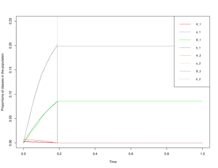
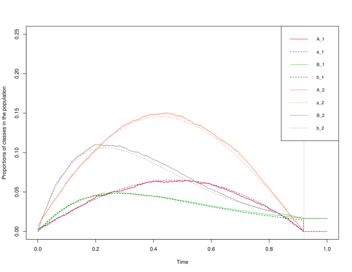
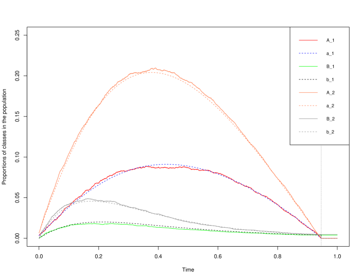
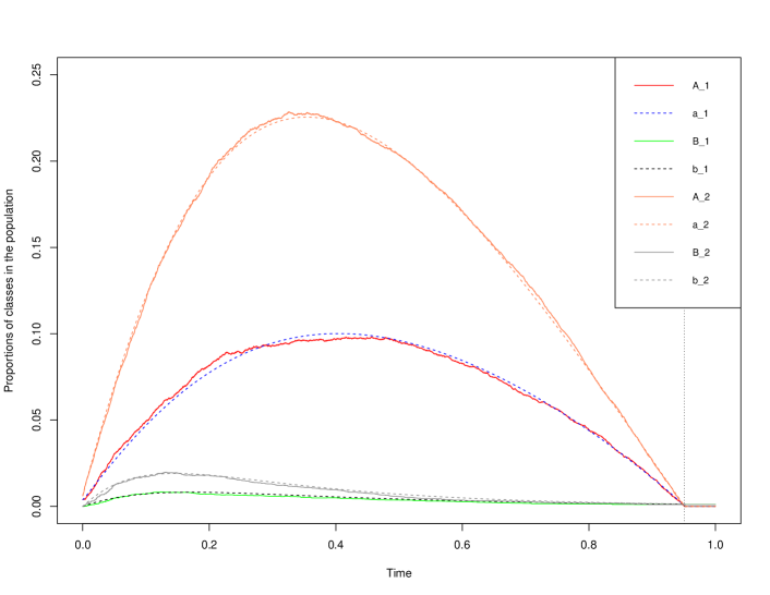
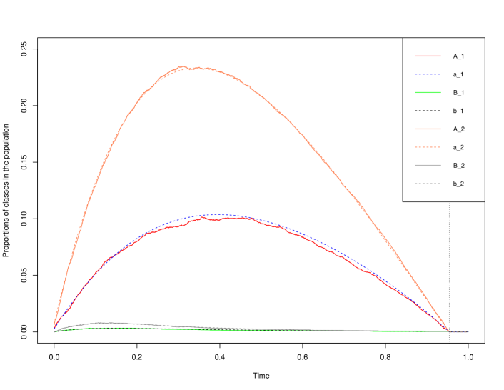
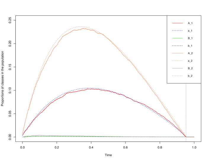
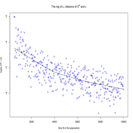
The simulations show that the deterministic solution of the system of ODEs (1.2) fits well with our stochastic process, see Figure 2. The sequence of stochastic process that we have constructed describes how the chain-referral process works on a network. When we consider the population with a very large number of people, the process is asymptotically a deterministic function, which is a solution of a system of (1.2). To see numerically the convergence, we do a simulation: for , we vary from 500 to 50000 and plot as a function of the of the quantity:
Figure 4. The speed of convergence has been studied in the case of Erdös-Rényi graphs in the PhD-thesis, by establishing a central limit theorem [28].
By studying the solution of (1.2), we can obtain an approximation of the fraction of the population that has been interviewed when the CRS process stops. The proportion of the population discovered is then approximated by .
The number of maximum coupon plays an important role in how many people we could explore before there is no distributed coupons any more (when ). By keeping all other parameters fixed and changing , in the simulations of Figure 2, we see that the time are different. For example, with , , , we obtain the table 1.
| c | 1 | 2 | 3 | 4 | 5 | 6 | … |
|---|---|---|---|---|---|---|---|
| 0.18 | 0.91 | 0.94 | 0.95 | 0.95 | 0.95 | … |
If , even though the average number of neighbors are bigger than , the simple random walk describing the survey reaches only a very small number of people, see Figure 2(a). The random walk stops when it encounters a node of degree 1 and can not propagate any more.
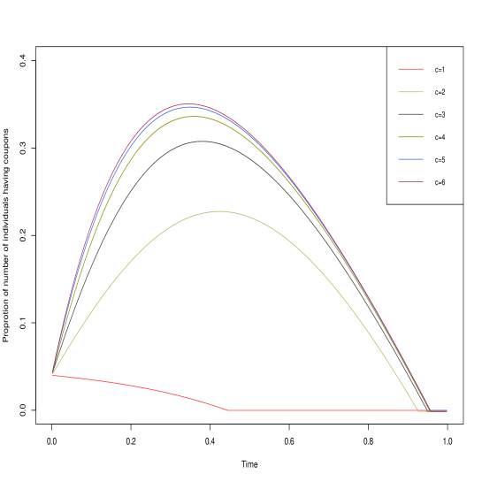
Furthermore, the parameter also impacts the peaks (time and size) the curves corresponding to the number of distributed coupons. In case of a limited budget with a fixed number of interviews, a higher value of can imply that we discover a larger fraction of the population since it allows more flexibility in the interviewees. From the Figure 5, we observe that the proportion of people receiving coupons gets bigger as increases. If , the fraction of discovered population is small, which means that the survey is not so efficient. When takes values from to , the corresponding curves of are ”close” and so are the times . However, in these cases, the number of coupons spent during the CRS survey is large. We can also be interested in seeing how impacts the part of population discovered when the survey stops after a fixed number of interviewed individuals. For example, consider the case when and assume that we start with . The parameters of the SBM are , . Then when there have been approximately individuals interviewed, the proportion of the explored individuals: for each varying from to is given in Table 2.
| c | 1 | 2 | 3 | 4 | 5 | 6 |
|---|---|---|---|---|---|---|
| 0.213 | 0.308 | 0.268 | 0.308 | 0.310 | 0.260 |
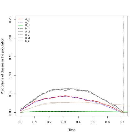
Changing the parameters impacts the discovered proportion of types. For instant, let us take a bipartite random model and , , which means that the people between communities are highly connected and there is no connection within community. In this case, the number of explored people without coupon of type 1 is quite small compared to the one of type 2, see Figure 3.
References
- [1] E. Abbe, Community detection and stochastic block models. Foundations and Trends® in Communications and Information Theory, 14(1-2):1–162, 2018.
- [2] K. B. Athreya and P. Jagers(eds.), Classical and modern branching processes. Volume 84. Springer Science & Business Media, 2012.
- [3] S. Athreya and A. Röllin, Respondent driven sampling and sparse graph convergence. arXiv e-prints, page arXiv:1705.02731, May 2017.
- [4] A. Bagheri and M. Saadati, Exploring the effectiveness of chain referral methods in sampling hidden populations. Indian Journal of Science and Technology, 8(30), 2015.
- [5] A. D. Barbour, L. Holst and S. Janson, Poisson approximation. Volume 2 of Oxford Studies in Probability. The Clarendon Press, Oxford University Press, New York, 1992. Oxford Science Publications.
- [6] A. Barbour and G. Reiner, Approximating the epidemic curve. Volume 2 of Oxford Studies in Probability. Electronic Journal of Probability 18, 2013.
- [7] B. Bollobás and O. Riordan Asymptotic Normality of the Size of the Giant Component via a Random Walk. Volume 102, Journal of Combinatorial Theory Serie B, pages 53–61, January 2012.
- [8] P. Billingsley, Convergence of Probability Measures. John Wiley & Sons, New York, 1968.
- [9] T. Britton and E. Pardoux, Stochastic Epidemic Models with Inference. Springer, 2019.
- [10] A. Cousien, J. S. Dhersin, V.C. Tran, and T. P. T. Vo, Respondent Driven Sampling on sparse Erdös-rényi graphs. in progress, 2019.
- [11] R. Durrett, Random graph dynamics. Volume 200, no. 7. Cambridge: Cambridge university press, 2007.
- [12] N. Enriquez, G. Faraud and L. Ménard, Limiting shape of the depth first search tree in an Erdös‐Rényi graph. Random Structures & Algorithms, 56(2), pp.501-516, 2020.
- [13] S. N. Ethier and T. G. Kurtz, Markov Processus, Characterization and Convergence. John Wiley & Sons, New York, 1986.
- [14] A. Gadde, E. E. Gad, S. Avestimehr, and A. Ortega, Active learning for community detection in stochastic block models. In 2016 IEEE International Symposium on Information Theory (ISIT), pages 1889–1893, July 2016.
- [15] M. Girvan and M. E. J. Newman, Community structure in social and biological networks. Proceedings of the national academy of sciences 99, no. 12: 7821–7826, 2002.
- [16] L. A. Goodman, Snowball sampling. The annals of mathematical statistics, pp.148–170, 1961.
- [17] D. D. Heckathorn, Respondent-driven Sampling: a new approach to the study of hidden populations. Social Problems, 44(1):74–99, 1997.
- [18] D. D. Heckathorn, Respondent-driven sampling II: Deriving valid population estimates from chain-referral samples of hidden populations. Social Problems, 49(1):11–34, 2002.
- [19] P. W. Holland, K. B. Laskey, and S. Leinhardt, Stochastic blockmodels: First steps. Social networks, 5(2):109–137, 1983.
- [20] A. Jakubowski, On the Skorokhod topology. Annales de l’Institut Henri Poincaré, 22(3):263–285, 1986.
- [21] S. Janson, M. Luczak and P. Windridge, Law of large numbers for the SIR epidemic on a random graph with given degrees. Random Structures & Algorithms, 45(4), pp.726-763, 2014.
- [22] A. Joffe and M. Métivier, Weak convergence of sequences of semimartingales with applications to multitype branching processes. Advances in Applied Probability, 18:20–65, 1986.
- [23] M. Métivier, Semimartingales: a course on stochastic processes. Volume 2. Walter de Gruyter, 2011.
- [24] E. Lazega and A. Bar-Hen and P. Barbillon and S. Donnet, Stochastic block models for multiplex networks: an application to networks of researchers. arXiv:1501.06444, 2015.
- [25] A. Shaghaghi and R. S. Bhopal and A. Sheikh, Approaches to recruiting ‘hard-to-reach’populations into research: a review of the literature. Health promotion perspectives, 1(2):86, 2011.
- [26] R. Van Der Hofstad, Random graphs and complex networks. Volume 1. Cambridge university press, 2016.
- [27] V. C. Tran, P. Moyal, L. Decreusefond and J. S. Dhersin, Limite en grand graphe d’un processus SIR décrivant la propagation d’une épidemie sur un réseau. Journées MAS et Journée en l’honneur de Jacques Neveu, Aug 2010, Talence, France.
- [28] T. P. T. Vo, Exploration of random graphs by the Respondent Driven Sampling method. PhD-Thesis, University Paris 13, 2020.