Anomalous $H\to ZZ\to 4\ell$ decay and its interference effects at the LHC

Abstract

We calculate the spinor helicity amplitudes of anomalous $H\to ZZ\to 4\ell$ decay. After embedding these analytic formulas into the MCFM package, we study the interference effects between the anomalous $gg\to H\to ZZ\to 4\ell$ process and the SM processes, which are indispensable in the Higgs off-shell region. Subsequently, the constraints on the anomalous couplings are estimated using LHC experimental data.

I Introduction

Since the 125 GeV/$c^{2}$ Higgs boson was discovered at the Large Hadron Collider (LHC) in 2012 Chatrchyan:2012xdj ; Aad:2012tfa , its properties have been tested more and more precisely Sirunyan:2018koj ; Tao:2018zeu ; Magnan:2018spp . Even though no new physics beyond Standard Model (SM) has been confirmed so far, it is still necessary and meaningful to search for new physics. In this paper we study the anomalous $HZZ$ couplings.

The new physics beyond the SM in the SM effective field theory (SMEFT) is shown as higher-dimensional operators in the Lagrangian which later supply non-SM interactions. In this analysis we note these non-SM $HVV$ ($V$ represents $Z,W,\gamma$) interactions from six-dimensional operators as anomalous $HVV$ couplings, and consider them separately from SM loop contributions. To scrutinize the Lorentz structures from several anomalous couplings, we calculate the scattering amplitudes in the spinor helicity method, and the analytic formulas are shown symmetrically and elegantly in the spinor notations.

$HVV$ couplings can be probed at the LHC through processes including $V^{\ast}\to VH$ or $H\to VV$ decays. Among these processes, the $gg\to H\to ZZ\to 4\ell$ process, which is called the golden channel, is the most precise and has been studied extensively in both theoretical studies  Gao:2010qx ; Bolognesi:2012mm ; Anderson:2013afp ; Chen:2012jy ; Chen:2013ejz ; Chen:2014pia ; Chen:2014hqs ; Nelson:1986ki ; Soni:1993jc ; Chang:1993jy ; Arens:1994wd ; Choi:2002jk ; Buszello:2002uu ; Godbole:2007cn ; Kovalchuk:2008zz ; Cao:2009ah ; DeRujula:2010ys ; Gainer:2011xz ; Coleppa:2012eh ; Stolarski:2012ps ; Boughezal:2012tz ; Avery:2012um ; Campbell:2012ct ; Campbell:2012cz ; Modak:2013sb ; Sun:2013yra ; Gainer:2013rxa ; Buchalla:2013mpa ; Chen:2013waa ; Kauer:2012hd ; Beneke:2014sba ; Falkowski:2014ffa ; Modak:2014zca ; Gonzalez-Alonso:2014rla ; Belyaev:2015xwa ; Gainer:2018qjm and experiments at LHC  Chatrchyan:2012jja ; Khachatryan:2014kca ; Khachatryan:2014iha ; deFlorian:2016spz ; Sirunyan:2017tqd ; Sirunyan:2019twz ; Aad:2015xua ; Aaboud:2018wps ; Aaboud:2018puo . Thus, we also choose this golden channel to study anomalous $HVV$ couplings. To reach a more precise result, both on-shell and off-shell Higgs regions can be exploited. At the same time, the interference effects between this process and the SM processes should be included. Especially in the off-shell Higgs region, the interference between this process and the continuum process $gg\to ZZ\to 4\ell$ should not be ignored Campbell:2013una ; Campbell:2011cu . Based on a modified MCFM Campbell:2013una ; Ellis:2014yca package with anomalous $HZZ$ couplings, we study the interference effects quantitatively. Furthermore, we estimate the constraints on the anomalous coupling using CMS experimental data at LHC.

The rest of the paper is organized as follows. In Section II, the spinor helicity amplitudes with anomalous couplings are calculated. In Section III, the analytic formulas are embedded into the MCFM8.0 package and the cross sections for proton - proton collision, especially the interference effects, are shown numerically. In Section  IV, the constraints on the $HZZ$ anomalous couplings are estimated. Section V is the conclusion and discussion.

II theoretical calculation

In this section firstly we introduce the $HZZ$ anomalous couplings, and then we calculate the spinor helicity amplitudes.

II.1 $HZZ$ anomalous couplings

In the SM effective field theory Buchmuller:1985jz ; Grzadkowski:2010es the complete form of higher-dimensional operators can be written as

$$\mathcal{L}=\mathcal{L}_{SM}+\frac{1}{\Lambda}\sum_{k}C_{k}^{5}\mathcal{O}_{k}^{5}+\frac{1}{\Lambda^{2}}\sum_{k}C_{k}^{6}\mathcal{O}_{k}^{6}+\mathcal{O}(\frac{1}{\Lambda^{3}})~{},$$ (1)

where $\Lambda$ is the new physics energy scale, and $C_{k}^{i}$ with $i=5,6$ are Wilson loop coefficients. As the dimension-five operators $\mathcal{O}_{k}^{5}$ have no contribution to anomalous $HZZ$ couplings, the dimension-six operators $\mathcal{O}_{k}^{6}$ have leading contributions. The relative dimension-six operators in the Warsaw basis Grzadkowski:2010es are

$$\mathcal{O}^{6}_{\Phi D}=(\Phi^{\dagger}D^{\mu}\Phi)^{\ast}(\Phi^{\dagger}D^{\mu}\Phi),$$

$$\mathcal{O}^{6}_{\Phi W}=\Phi^{\dagger}\Phi W^{I}_{\mu\nu}W^{I\mu\nu},~{}~{}\mathcal{O}^{6}_{\Phi B}=\Phi^{\dagger}\Phi B_{\mu\nu}B^{\mu\nu},~{}~{}\mathcal{O}^{6}_{\Phi WB}=\Phi^{\dagger}\tau^{I}\Phi W^{I}_{\mu\nu}B^{\mu\nu},$$

$$\mathcal{O}^{6}_{\Phi\tilde{W}}=\Phi^{\dagger}\Phi\tilde{W}^{I}_{\mu\nu}W^{I\mu\nu},~{}~{}\mathcal{O}^{6}_{\Phi\tilde{B}}=\Phi^{\dagger}\Phi\tilde{B}_{\mu\nu}B^{\mu\nu},~{}~{}\mathcal{O}^{6}_{\Phi\tilde{W}B}=\Phi^{\dagger}\tau^{I}\Phi\tilde{W}^{I}_{\mu\nu}B^{\mu\nu},$$ (2)

where $\Phi$ is a doublet representation under the $SU(2)_{L}$ group and the aforementioned Higgs field $H$ is one of its four components; $D_{\mu}=\partial_{\mu}-igW^{I}_{\mu}T^{I}-ig^{\prime}YB_{\mu}$, where $g$ and $g^{\prime}$ are coupling constants, $T^{I}=\tau^{I}/2$, where $\tau^{I}$ are Pauli matrices, $Y$ is the $U(1)_{Y}$ generator; $W^{I}_{\mu\nu}=\partial_{\mu}W^{I}_{\nu}-\partial_{\nu}W^{I}_{\mu}-g\epsilon^{IJK}W^{J}_{\mu}W^{K}_{\nu}$, $B_{\mu\nu}=\partial_{\mu}B_{\nu}-\partial_{\nu}B_{\mu}$, $\tilde{W}^{I}_{\mu\nu}=\frac{1}{2}\epsilon_{\mu\nu\rho\sigma}W^{I\rho\sigma}$, $\tilde{B}_{\mu\nu}=\frac{1}{2}\epsilon_{\mu\nu\rho\sigma}B^{\rho\sigma}$.

For the $H\to 4\ell$ process that we are going to take to constrain the anomalous $HZZ$ couplings numerically, there are dimension-six operators include $HZ\ell\ell$ contact interaction  Barklow:2017awn ; Cohen:2016bsd that can also contribute non-SM effects, which are

$$\mathcal{O}^{6}_{\Phi L}=(\Phi^{\dagger}\mbox{$\raisebox{5.69054pt}{\boldmath${}^{\leftrightarrow}$}D$}_{\mu}\Phi)(\bar{L}\gamma_{\mu}L),~{}~{}\mathcal{O}^{6}_{\Phi LT}=(\Phi^{\dagger}T^{I}\mbox{$\raisebox{5.69054pt}{\boldmath${}^{\leftrightarrow}$}D$}_{\mu}\Phi)(\bar{L}\gamma_{\mu}T^{I}L),~{}~{}\mathcal{O}^{6}_{\Phi e}=(\Phi^{\dagger}\mbox{$\raisebox{5.69054pt}{\boldmath${}^{\leftrightarrow}$}D$}_{\mu}\Phi)(\bar{e}\gamma_{\mu}e),$$ (3)

where $\Phi^{\dagger}\mbox{$\raisebox{5.69054pt}{\boldmath${}^{\leftrightarrow}$}D$}_{\mu}\Phi=\Phi^{\dagger}D_{\mu}\Phi-D_{\mu}\Phi^{\dagger}\Phi$,   $\Phi^{\dagger}T^{I}\mbox{$\raisebox{5.69054pt}{\boldmath${}^{\leftrightarrow}$}D$}_{\mu}\Phi=\Phi^{\dagger}T^{I}D_{\mu}\Phi-D_{\mu}\Phi^{\dagger}T^{I}\Phi$, $L$,$e$ represent left- and right-handed charged leptons. One may worry about the pollution caused by the $HZ\ell\ell$ contact interaction from these operators to the $4\ell$ final state when probing $HZZ$ couplings. Nevertheless, we can use certain additional methods to distinguish them. In the off-shell Higgs region, the on-shell $Z$ boson selection cut can reduce much of the $HZ\ell\ell$ background. In on-shell Higgs region, the non-leptonic $Z$ decay channel can also be adopted in constraining $HZZ$ couplings. These discussions are not the focus of the current paper and we are not going to examine them in detail here.

After spontaneous symmetry breaking, we get the anomalous $HZZ$ interactions

$$\mathcal{L}_{a}=\frac{a_{1}}{v}M_{Z}^{2}HZ^{\mu}Z_{\mu}-\frac{a_{2}}{v}HZ^{\mu\nu}Z_{\mu\nu}-\frac{a_{3}}{v}HZ^{\mu\nu}\tilde{Z}_{\mu\nu}~{},$$ (4)

with

$$a_{1} = \frac{v^{2}}{\Lambda^{2}}C^{6}_{\Phi D},$$

$$a_{2} = -\frac{v^{2}}{\Lambda^{2}}(C^{6}_{\Phi W}c^{2}+C^{6}_{\Phi B}s^{2}+C^{6}_{\Phi WB}cs),$$

$$a_{3} = -\frac{v^{2}}{\Lambda^{2}}(C^{6}_{\Phi\tilde{W}}c^{2}+C^{6}_{\Phi\tilde{B}}s^{2}+C^{6}_{\Phi\tilde{W}B}cs),$$ (5)

where $c$ and $s$ stand for the cosine and sine of the weak mixing angle respectively, $a_{1},a_{2},a_{3}$ are dimensionless complex numbers and $v=246$ GeV is the electroweak vacuum expectation value. Notice that the signs before $a_{2}$ and $a_{3}$ are same as in Gao:2010qx ; Khachatryan:2014kca ; Sirunyan:2019twz , but have an additional minus sign from the definition in Chen:2013ejz . $Z_{\mu}$ is $Z$ boson field, $Z_{\mu\nu}=\partial_{\mu}Z_{\nu}-\partial_{\nu}Z_{\mu}$ is the field strength tensor of the $Z$ boson and $\tilde{Z}_{\mu\nu}=\frac{1}{2}\epsilon_{\mu\nu\rho\sigma}Z^{\rho\sigma}$ represents its dual field strength. The loop corrections in SM can contribute similarly as the $a_{2}$ and $a_{3}$ terms. Quantitatively, the one-loop correction can contribute to $a_{2}$ term with small contributions $\mathcal{O}(10^{-2}-10^{-3})$, while the $a_{3}$ term appear in SM only at a three-loop level and thus has a even smaller contribution Khachatryan:2014kca . Therefore, only if the contributions from the $a_{2}$ and $a_{3}$ terms are larger than these loop contributions can we consider them as from new physics.

The $HZZ$ interaction vertex from Eq. (4) is

$$\Gamma_{a}^{\mu\nu}(k,k^{\prime})=i\frac{2}{v}\sum_{i=1}^{3}a_{i}\Gamma_{a,i}^{\mu\nu}(k,k^{\prime})=i\frac{2}{v}[a_{1}M_{Z}^{2}g^{\mu\nu}-2a_{2}(k^{\nu}k^{\prime\mu}-k\cdot k^{\prime}g^{\mu\nu})-2a_{3}\epsilon^{\mu\nu\rho\sigma}k_{\rho}k^{\prime}_{\sigma}]~{},$$ (6)

where $k$,$k^{\prime}$ are the momenta of the two $Z$ bosons. It is worthy to notice that the $HZZ$ vertices in the SM are

$$\Gamma_{\text{SM}}^{\mu\nu}(k,k^{\prime})=i\frac{2}{v}M_{Z}^{2}g^{\mu\nu}~{},$$ (7)

so the Lorentz structure of the $a_{1}$ term is same as the SM case. While the $a_{2}$ and $a_{3}$ terms have different Lorentz structures, which represent non-SM $CP$-even and $CP$-odd cases respectively.

II.2 Helicity amplitude of the process $gg\rightarrow H\rightarrow ZZ\to 2e2\mu$

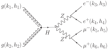
Figure 1: Feynman diagram of the Higgs-mediated process $gg\rightarrow H\rightarrow ZZ\to 2e2\mu$. The black dot represents an effective $ggH$ coupling from loop contributions.

The total helicity amplitude for the process $gg\rightarrow H\rightarrow ZZ\to 2e2\mu$ in Fig. 1 is composed of three individual amplitudes $A^{H}_{\rm SM},A^{H}_{CP-\rm{even}}$ and $A^{H}_{CP-\rm{odd}}$, which have the same production process but different Higgs decay modes according to the three kinds of $HZZ$ vertices in Eq. (6). The specific formulas are

$$~{}~{}~{}~{}\mathcal{A}^{gg\to H\rightarrow ZZ\to 2e2\mu}(1_{g}^{h_{1}},2_{g}^{h_{2}},3_{e^{-}}^{h_{3}},4^{h_{4}}_{e^{+}},5_{\mu^{-}}^{h_{5}},6^{h_{6}}_{\mu^{+}})$$ (8)

$$=[a_{1}\mathcal{A}^{H}_{\rm SM}+a_{2}\mathcal{A}^{H}_{CP-\rm{even}}+a_{3}\mathcal{A}^{H}_{CP-\rm{odd}}](1_{g}^{h_{1}},2_{g}^{h_{2}},3_{e^{-}}^{h_{3}},4^{h_{4}}_{e^{+}},5_{\mu^{-}}^{h_{5}},6^{h_{6}}_{\mu^{+}})~{},$$ (9)

$$=\mathcal{A}^{gg\rightarrow H}(1_{g}^{h_{1}},2_{g}^{h_{2}})\times\frac{P_{H}(s_{12})}{s_{12}}\times\sum_{i=1}^{3}a_{i}\mathcal{A}_{i}^{H\rightarrow ZZ\to 2e2\mu}(3_{e^{-}}^{h_{3}},4^{h_{4}}_{e^{+}},5_{\mu^{-}}^{h_{5}},6^{h_{6}}_{\mu^{+}})~{},$$ (10)

where $h_{i}$ $(i=1\cdots 6)$ are helicity indices of external particles, $s_{ij}=(k_{i}+k_{j})^{2}$ and $P_{H}(s)=\frac{s}{s-M_{H}^{2}+iM_{H}\Gamma_{H}}$ is the Higgs propagator.

The production part $\mathcal{A}^{gg\to H}(1^{h_{1}}_{g},2^{h_{2}}_{g})$ is the helicity amplitude of gluon-gluon fusion to Higgs process, in which $h_{1},h_{2}$ represent the helicities of gluons with outgoing momenta. For all the other helicity amplitudes in this paper, we also keep the convention that the momentum of each external particle is outgoing. When writing the helicity amplitudes, we adopt the conventions used in Dixon:1996wi ; Campbell:2013una :

$$\langle ij\rangle=\bar{u}_{-}(p_{i})u_{+}(p_{j}),\qquad~{}~{}{[ij]}=\bar{u}_{+}(p_{i})u_{-}(p_{j})~{},$$

$$\langle ij\rangle[ji]=2p_{i}\cdot p_{j},\qquad~{}~{}s_{ij}=(p_{i}+p_{j})^{2},$$ (11)

and we have

$$\mathcal{A}^{gg\to H}(1^{+}_{g},2^{+}_{g}) = \frac{2c_{g}}{v}[12]^{2}~{},$$

$$\mathcal{A}^{gg\to H}(1^{-}_{g},2^{-}_{g}) = \frac{2c_{g}}{v}\langle 12\rangle^{2}~{}.$$ (12)

To keep the $ggH$ coupling consistent with SM, we make

$$\frac{c_{g}}{v}=\frac{1}{2}\sum_{f}\frac{\delta^{ab}}{2}\frac{i}{16\pi^{2}}g^{2}_{s}4e\frac{m_{f}^{2}}{2M_{W}s_{W}}\frac{1}{s_{12}}[2+s_{12}(1-\tau_{H})C^{\gamma\gamma}_{0}(m_{f}^{2})]~{},$$ (13)

with

$$C^{\gamma\gamma}_{0}(m^{2})=2\tau_{H}f(\tau_{H})/4m^{2}~{},\tau_{H}=4m^{2}/M^{2}_{H},$$ (14)

$$f(\tau)=\left\{\begin{array}[]{ll}{\rm arcsin}^{2}\sqrt{1/\tau}&\tau\geq 1\\ -\frac{1}{4}\left[\log\frac{1+\sqrt{1-\tau}}{1-\sqrt{1-\tau}}-i\pi\right]^{2}&\tau<1{}\end{array}\right.~{},$$ (15)

where $a,b=1,...,8$ are $SU(3)_{c}$ adjoint representation indices for the gluons, the index $f$ represents quark flavor and $C^{\gamma\gamma}_{0}(m^{2})$ is the Passarino-Veltman three-point scalar function Passarino:1978jh ; Chen:2017plj .

The decay part $\mathcal{A}^{H\rightarrow ZZ\to 2e2\mu}(3_{e^{-}}^{h_{3}},4^{h_{4}}_{e^{+}},5_{\mu^{-}}^{h_{5}},6^{h_{6}}_{\mu^{+}})$ is the helicity amplitude of the process $H\rightarrow ZZ\to e^{-}e^{+}\mu^{-}\mu^{+}$, which have three sources according to the three types of vertices as written in Eq. (6). Correspondingly we write it as

$$\mathcal{A}^{H\rightarrow ZZ\to 2e2\mu}(3_{e^{-}}^{h_{3}},4^{h_{4}}_{e^{+}},5_{\mu^{-}}^{h_{5}},6^{h_{6}}_{\mu^{+}})=\sum_{i=1}^{3}a_{i}\mathcal{A}_{i}^{H\rightarrow ZZ\to 2e2\mu}(3_{e^{-}}^{h_{3}},4^{h_{4}}_{e^{+}},5_{\mu^{-}}^{h_{5}},6^{h_{6}}_{\mu^{+}})$$ (16)

with

$$\mathcal{A}_{1}^{H\rightarrow ZZ\to 2e2\mu}(3^{-}_{e^{-}},4^{+}_{e^{+}},5^{-}_{\mu^{-}},6^{+}_{\mu^{+}})=f\times l^{2}_{e}\frac{M_{W}^{2}}{\cos^{2}\theta_{W}}\langle 35\rangle[46],$$ (17)

$$\mathcal{A}_{2}^{H\rightarrow ZZ\to 2e2\mu}(3^{-}_{e^{-}},4^{+}_{e^{+}},5^{-}_{\mu^{-}},6^{+}_{\mu^{+}})=f\times l^{2}_{e}\times$$

$$\Big{[}2k\cdot k^{\prime}\langle 35\rangle[46]+\big{(}\langle 35\rangle[45]+\langle 36\rangle[46]\big{)}\big{(}\langle 35\rangle[36]+\langle 45\rangle[46]\big{)}\Big{]},$$ (18)

$$\mathcal{A}_{3}^{H\rightarrow ZZ\to 2e2\mu}(3^{-}_{e^{-}},4^{+}_{e^{+}},5^{-}_{\mu^{-}},6^{+}_{\mu^{+}})=f\times l^{2}_{e}\times(-i)\times$$

$$\Big{[}2\big{(}k\cdot k^{\prime}+\langle 46\rangle[46]\big{)}\langle 35\rangle[46]+\langle 35\rangle[45]\big{(}\langle 35\rangle[36]+\langle 45\rangle[46]\big{)}$$

$$+\langle 36\rangle[46]\big{(}\langle 35\rangle[36]-\langle 45\rangle[46]\big{)}\Big{]}~{}.$$ (19)

and

$$f=-2ie^{3}\frac{1}{M_{W}\sin\theta_{W}}\frac{P_{Z}(s_{34})}{s_{34}}\frac{P_{Z}(s_{56})}{s_{56}}~{},$$ (20)

where $P_{Z}(s)=\frac{s}{s-M_{Z}^{2}+iM_{Z}\Gamma_{Z}}$ is the $Z$ boson propagator, $M_{Z}$,$M_{W}$ are the masses of the $Z$,$W$ bosons, $\theta_{W}$ is the Weinberg angle, $l_{e}$ and $r_{e}$ ( will appear for other helicity combinations) are the coupling factors of the $Z$ boson to left-handed and right-handed leptons:

$$l_{e}=\frac{-1+2\sin^{2}\theta_{W}}{\sin(2\theta_{W})}~{},r_{e}=\frac{2\sin^{2}\theta_{W}}{\sin(2\theta_{W})}~{}.$$ (21)

In Eq.s (17)(LABEL:eqn:amp2)(19), we only show the case in which the helicities of the four leptons ($h_{3},h_{4},h_{5},h_{6}$) are equal to ($-,+,-,+$). As for the other three non-zero helicity combinations ($-,+,+,-$), ($+,-,-,+$), ($+,-,+,-$), their helicity amplitudes are similar to Eq.s (17)(LABEL:eqn:amp2)(19), but with some exchanges such as

$$l_{e}\leftrightarrow r_{e}~{},~{}4\leftrightarrow 6~{},~{}3\leftrightarrow 5~{},~{}[]\leftrightarrow\langle\rangle~{}.$$ (22)

Their specific formulas are shown in Appendix A.

II.3 Helicity amplitude of the box process $gg\rightarrow ZZ\to 2e2\mu$

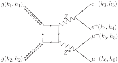
Figure 2: Feynman diagram of the box process $gg\rightarrow ZZ\to 2e2\mu$ .

The box process $gg\rightarrow ZZ\to 2e2\mu$ is a continuum background of the Higgs-mediated $gg\to H\to 2e2\mu$ process. The interference between these two kinds of processes can have nonnegligible contribution in the off-shell Higgs region. The Feynman diagram of the process $gg\rightarrow ZZ\to 2e2\mu$ is a box diagram which is induced by fermion loops (see Fig. 2). The helicity amplitude $A^{gg\rightarrow ZZ\to 2e2\mu}_{\text{box}}$ has been calculated analytically and coded in MCFM8.0 package. Another similar calculation that using a different method can be found in gg2VV code Binoth:2008pr .

II.4 Helicity amplitude of the process $gg\rightarrow H\rightarrow ZZ\to 4\ell$

The process $gg\rightarrow H\rightarrow ZZ\to 4\ell$ with identical $4e$ or $4\mu$ final states can also be used to probe the anomalous $HZZ$ couplings. In SM the differential cross sections of the $4\ell$ (include both $4e$ and $4\mu$ ) and $2e2\mu$ processes are nearly the same in both on-shell and off-shell Higgs regions Ellis:2014yca , which indicates adding the $4e/4\mu$ process can almost double experimental statistics. This situation can probably be similar for the anomalous Higgs-mediated processes. The $4e/4\mu$ Feynman diagrams consist of two different topology structures as shown in Fig. 3. Fig. 3(b) is different from Fig. 3(a) just by swapping the positive charged leptons (4$\leftrightarrow$6). The helicity amplitude of each diagram is similar to the former $2e2\mu$ cases but need to be multiplied by a symmetry factor $\frac{1}{2}$. While calculating the total cross section the interference term between Fig. 3(a) and (b) need an extra factor of -1 comparing to the self-conjugated terms because it connects all of the decayed leptons in one fermion loop while each self-conjugated term has two fermion loops. After considering these details, the summed cross section of $4e$ and $4\mu$ processes is comparable to the $2e2\mu$ process. More details are shown in the following numerical results.

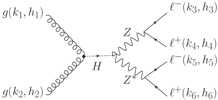
(a)

(b)

Figure 3: The Feynman diagrams of the process $gg\rightarrow H\rightarrow ZZ\to 4\ell$, where $4\ell=4e\ \mbox{or}\ 4\mu$. Note that diagram (b) is obtained by swapping the two positive charged leptons (4$\leftrightarrow$6) in diagram (a).

III Numerical result

In this section we present the integrated cross sections and differential distributions in both on-shell and off-shell Higgs regions, especially the interference between anomalous Higgs-mediated processes and SM processes.

III.1 The cross sections

To compare theoretical calculation with experimental observation at LHC, we need to further calculate the cross sections at hadron level. From helicity amplitude to the cross section, there need two more steps. Firstly we should sum and square the amplitudes to get the differential cross section at parton level, then integrate phase space and parton distribution function (PDF) to get the cross section at hadron level. As following we show these two steps conceptually.

The squared amplitude in the differential cross section at parton level $d\hat{\sigma}(s_{12})$ is

$$\left|\mathcal{A}_{\text{box}}^{gg\to ZZ\to 4\ell}+\mathcal{A}^{gg\to H\to ZZ\to 4\ell}\right|^{2}$$ (23)

$$= \left|\mathcal{A}_{\text{box}}^{gg\to ZZ\to 4\ell}+\mathcal{A}^{H}_{\rm SM}+a_{1}\mathcal{A}^{H}_{\rm SM}+a_{2}\mathcal{A}^{H}_{CP-\rm{even}}+a_{3}\mathcal{A}^{H}_{CP-\rm{odd}}\right|^{2}~{}.$$ (24)

After expanding it, there left self-conjugated terms and interference terms that have different amplitude sources. As in the next step the integral of phase space and PDF are same for each term, we note the integrated cross sections separately by the amplitude sources, which are

$$\sigma_{k,l}\sim\left\{\begin{array}[]{ll}|\mathcal{A}_{k}|^{2},&k=l;\\ 2\text{Re}(\mathcal{A}^{\ast}_{k}\mathcal{A}_{l}),&k\neq l,\\ \end{array}\right.$$ (25)

where $k,l=$ {box, SM, $CP$-even, $CP$-odd}. The superscripts of $\mathcal{A}$ are omitted for brevity.

III.2 Numerical results for $gg\to 2e2\mu$ process

We make the integral of phase space and the PDF in the MCFM 8.0 package Campbell:2015qma ; Boughezal:2016wmq . The simulation is performed for the proton-proton collision at the center-of-mass energy $\sqrt{s}=13$ TeV. The Higgs mass is set to be $M_{H}=125\rm~{}GeV$. The renormalization $\mu_{r}$ and factorization scale $\mu_{f}$ are set as the dynamic scale $m_{4\ell}/2$. For PDF we choose the leading-order MSTW 2008 PDFs MSTW08LO Martin:2009iq . Some basic phase space cuts are exerted as follows, which are similar to the event selection cuts used in CMS experiment CMS-PAS-HIG-13-002 .

$$P_{T,\mu}>5\rm~{}GeV,\ |\eta_{\mu}|<2.4~{},$$ (26)

$$P_{T,e}>7\rm~{}GeV,\ |\eta_{e}|<2.5~{},$$

$$\ m_{\ell\ell}>4\rm~{}GeV,\ m_{4\ell}>100\rm~{}GeV~{}.$$

Besides, for the $2e2\mu$ channel, the hardest (second-hardest) lepton should satisfy $P_{T}>20~{}(10)\rm~{}GeV$; one pair of leptons with the same flavour and opposite charge is required to have $40\rm~{}GeV<m_{\ell^{+}\ell^{-}}<120\rm~{}GeV$ and the other pair needs to fulfill $12\rm~{}GeV<m_{\ell^{+}\ell^{-}}<120\rm~{}GeV$. For the $4e$ or $4\mu$ channel, four oppositely charge lepton pairs exist as $Z$ boson candidates. The selection strategy is to first choose one pair nearest to the $Z$ boson mass as one $Z$ boson, then consider the left two leptons as the other $Z$ boson. The other requirements are similar to the $2e2\mu$ channel.

13 TeV, $m_{2e2\mu}<130\rm~{}GeV$, on-shell
$\sigma_{k,l}$(fb)		box	Higgs-med.
			SM	$CP$-even	$CP$-odd
box		0.024	0	0	0
Higgs-med.	SM	0	0.503	0.558	0
	$CP$-even	0	0.558	0.202	0
	$CP$-odd	0	0	0	0.075

13 TeV, $m_{2e2\mu}>220\rm~{}GeV$, off-shell
$\sigma_{k,l}$(fb)		box	Higgs-med.
			SM	$CP$-even	$CP$-odd
box		1.283	-0.174	-0.571	0
Higgs-med.	SM	-0.174	0.100	0.137	0
	$CP$-even	-0.571	0.137	0.720	0
	$CP$-odd	0	0	0	0.716

Table 1: The cross sections of $gg\to 2e2\mu$ processes in proton-proton collision at center-of-mass energy $\sqrt{s}=13$ TeV with $a_{1}=0,a_{2}=a_{3}=1$ in Eq. (6).

Table 1 shows the cross sections $\sigma_{k,l}$ with $k,l=$ {box, SM, $CP$-even, $CP$-odd} while $a_{1},a_{2},a_{3}$ are all set to 1 for convinience. The cross section values can be converted easily by multiplying a scale factor for small $a_{i}$s. In the left and right panels, the integral regions of $m_{4\ell}$ are separately set as $m_{4\ell}<130~{}\text{GeV}$ and $m_{4\ell}>220~{}\text{GeV}$, which correspond to the on-shell and off-shell Higgs regions, respectively. Next we focus on two kinds of interference effects: the interference between each Higgs-mediated process and box continuum background, denoted as $\sigma_{\text{box},l}$ (or $\sigma_{l,\text{box}}$) with $l\neq\text{box}$; and the interference between different Higgs-mediated processes, denoted as $\sigma_{k,l}$ with $k,l\neq{\rm box}$.

The interference terms between Higgs-mediated processes and the continuum background $\sigma_{\text{box},l}$ are all zeros in on-shell Higgs region, but relatively sizeble in the off-shell regions except for the cases with the $CP$-odd Higgs-mediated process as shown in Table 1. There is an interesting reason for it. As from Eq. (9)(10)(25),

$$\sigma_{\text{box},l} \sim 2\text{Re}(\mathcal{A}^{\ast}_{\text{box}}\mathcal{A}_{l})~{},$$ (27)

$$\sim 2\text{Re}\big{(}\mathcal{A}^{\ast}_{\rm box}\mathcal{A}^{gg\to H}P_{H}(s_{12})\mathcal{A}_{i}\big{)}~{},$$

$$\sim 2\frac{(s_{12}-M^{2}_{H})\text{Re}\big{(}\mathcal{A}^{\ast}_{\rm box}\mathcal{A}^{gg\to H}\mathcal{A}_{i}\big{)}+M_{H}\Gamma_{H}\text{Im}\big{(}\mathcal{A}^{\ast}_{\rm box}\mathcal{A}^{gg\to H}\mathcal{A}_{i}\big{)}}{(s_{12}-M^{2}_{H})^{2}+M^{2}_{H}\Gamma^{2}_{H}}~{},$$

which means the integrand of $\sigma_{\text{box},l}$ consists of two parts, one is antisymmetric around $M^{2}_{H}$, the other is proportional to $M_{H}\Gamma_{H}\text{Im}\big{(}\mathcal{A}^{\ast}_{\rm box}\mathcal{A}^{gg\to H}\mathcal{A}_{i}\big{)}$. The first part can be largely suppressed almost to zero in the integral with an integral region symmetric around $M_{H}$. The second part is also suppressed not only by the small factor of $\Gamma_{H}/M_{H}$ but also by a small value of $\text{Im}\big{(}\mathcal{A}^{\ast}_{\rm box}\mathcal{A}^{gg\to H}\mathcal{A}_{i}\big{)}$ in the on-shell Higgs region. By contrary, in the off-shell Higgs region the integral regions are not symmetric around $M_{H}$ but in one side larger than $M_{H}$, which makes the first term have some non-zero contribution. Both the first and the second terms can also be enhanced when $\sqrt{s_{12}}$ is a little larger than twice of the top quark mass. That is because the $gg\to H$ process is induced mainly by top quark loop, both the real part and the imaginary part of the amplitude (Re$\mathcal{A}^{gg\to H}$ and Im$\mathcal{A}^{gg\to H}$) can be enhanced when $\sqrt{s_{12}}$ is just larger than the $2M_{t}$ threshold (see Eq. (13)). Then $\text{Im}\big{(}\mathcal{A}^{\ast}_{\rm box}\mathcal{A}^{gg\to H}\mathcal{A}_{i}\big{)}$ can have a larger value, even though the relative contribution from the second term can be still suppressed by the smallness of the factor $\Gamma_{H}/M_{H}$. In conclusion, mainly due to the nonsymmetric integral region and some enhancement of $\mathcal{A}^{gg\to H}$, the interferece contribution in the off-shell Higgs region becomes comparable with the self-conjugated contributions.

It is also worthwhile to point out there is no cross section contribution from the interference between the $CP$-odd Higgs-mediated process and other three processes, which include the continuumm background process, SM Higgs-mediated process and anomalous $CP$-even Higgs-mediated process. It is because there is an antisymmetric tensor $\epsilon^{\mu\nu\rho\sigma}$ in the $CP$-odd $HZZ$ interaction vertex (see last term in Eq. (6)), while in the other three processes, the two indices are symmetrically paired and so the contract of the indices makes the interference term zero. Nevertheless, these $CP$-odd interference term can show angular distributions, include polar angle distribution of $\ell$ in $Z$ boson rest frame and azimuthal angular distribution between two $z$ decay planes Buchalla:2013mpa ; Beneke:2014sba , even though its contribution to the total cross scetion is still zero.

The interference between $CP$-even Higgs-mediated process and SM Higgs-mediated process is nonnegligible both in on-shell and off-shell Higgs regions. In on-shell Higgs region, the contribution from interfernce terms is larger than that from the self-conjugated terms. Furthermore, for $a_{1}=0,a_{2}=-1$ choice(as in Chen:2013ejz ), the interference terms would have a minus sign, comparing to the relative values in Table 1, which makes the total contribution of $CP$-even Higgs-mediated process beyond SM a destructive effect. In the off-shell region, the $CP$-even Higgs-mediated process have two interference terms, separately between SM Higgs-mediated process and the box process. These two interference terms have opposite sign, which means they cancel each other partly. Even though, the summed interfernce effect is still comparable to the self-conjugated contribution.

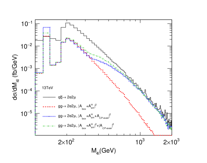
Figure 4: Differential cross sections of the $gg\to 2e2\mu$ processes and $q\bar{q}\to 2e2\mu$ process in proton-proton collision at $\sqrt{s}=13$ TeV with $a_{2}=1,a_{1}=a_{3}=0$ in Eq. (6).

Fig. 4 shows the differential cross sections. The black histogram is from its main background process $q\bar{q}\to 2e2\mu$, which is a huge background but still controllable. The red dashed histogram is from the SM $gg\to 2e2\mu$ processes including contributions from both the box and SM Higgs-mediated amplitudes. The blue dotted histogram adds contribution from the $CP$-even Higgs-mediated amplitude to the SM signal and background amplitudes. Therefore three kinds of interference terms are included. For comparison, we also show the green dashed-dotted histogram without interference terms from $CP$-even Higgs amplitudes with others, so the interference contribution can be calculated by the difference between blue and green histograms. In the on-shell region we can see the $CP$-even Higgs-mediated process have a total positive contribution (blue histogram) compare to the SM process(red histogram), while the green histogram shows the main positive contribution is from the interference term. In the off-shell region, the interference contribution is obvious in $200~{}\rm GeV<m_{4\ell}<600~{}\rm GeV$ region. There is a bump in blue and green histograms when $m_{4\ell}\approx 350$ GeV, which is caused by the total cross section of the $CP$-even Higgs-mediated process increase suddenly beyond the $2M_{t}$ (twice of the top quark mass) threshold. The differential cross section for the $CP$-odd Higgs-mediated process is similar to the green histogram in off-shell region since it has no interference contribution after the angular distributions being integrated.

The numerical results at center-of-mass energy $\sqrt{s}=8$ TeV are shown in Table 3 in Appendix B. By comparing them to the results at $\sqrt{s}=13$ TeV in Table 1, we can find that each cross section is decreased by about one or two times and their relative ratios have some minor changes. That can be caused by both PDF functions and kinematic distributions.

III.3 Numerical results for $gg\to 4e/4\mu$ processes

13 TeV, $m_{4e/4\mu}<130\rm~{}GeV$, on-shell
$\sigma_{k,l}$(fb)		box	Higgs-med.
			SM	$CP$-even	$CP$-odd
box		0.045	0	0	0
Higgs-med.	SM	0	0.540	0.568	0
	$CP$-even	0	0.568	0.186	0
	$CP$-odd	0	0	0	0.060

13 TeV, $m_{4e/4\mu}>220\rm~{}GeV$, off-shell
$\sigma_{k,l}$(fb)		box	Higgs-med.
			SM	$CP$-even	$CP$-odd
box		1.303	-0.176	-0.575	0
Higgs-med.	SM	-0.176	0.101	0.137	0
	$CP$-even	-0.575	0.137	0.740	0
	$CP$-odd	0	0	0	0.708

Table 2: Cross sections of $gg\to 4e/4\mu$ processes in proton-proton collisions at center-of-mass energy $\sqrt{s}=13$ TeV with $a_{1}=0,a_{2}=a_{3}=1$ in Eq. (6).

The cross sections of $gg\to 4e/4\mu$ processes are listed in Table 2 (Table 4 in Appendix B) for comparison and next use. Here $gg\to 4e/4\mu$ represents the sum of $gg\to 4e$ and $gg\to 4\mu$. Comparing Table 2 with Table 1, the numbers in the right panels are similar, while the numbers in the left panels have relatively large differences. That is mainly because the different selection cuts Ellis:2014yca . If apply the $4e/4\mu$ selection cuts to the $gg\to 2e2\mu$ process, $\sigma_{\rm box,box}$ in the left panels can become similar.

IV Constraints: a naive estimation

In this section we show a naive estimation to constrain $a_{1}$, $a_{2}$ and $a_{3}$ by using the data in both the on-shell and off-shell Higgs regions.

First, we estimate the expected number of events $N^{\rm exp}(a_{1},a_{2},a_{3})$ in the off-shell Higgs region, which is defined as the contribution from the processes with anomalous couplings after excluding the pure SM contributions.

A theoretical observed total number of events should be

$$N^{\rm theo}(a_{1},a_{2},a_{3})=\sigma_{\rm tot}\times\mathcal{L}\times k\times\epsilon~{},$$ (28)

where $\sigma_{\rm tot}$ is the total cross section, $\mathcal{L}$ is the integrated luminosity, $k$ represents the $k$-factor and $\epsilon$ is the total efficiency.

The simulation in the CMS experiment Sirunyan:2019twz with an integrated luminosity of $\mathcal{L}\sim 80$ fb^-1 at $\sqrt{s}=13$ TeV shows that for the $gg\to 4\ell$ process, the expected numbers of events in the off-shell Higgs region ($m_{4\ell}>220\rm~{}GeV$) can be divided into two categories: $N_{gg~{}~{}{\rm signal}}=20.3$ and $N_{gg~{}~{}{\rm interference}}=-34.4$, where the subscript “$gg$ signal” represents the SM Higgs-mediated signal term, “$gg$ interference” represents the interference term between SM Higgs-mediated process and the box process. For high-order corrections that may change the $k$-factor, some existing studies Caola:2015psa ; Melnikov:2015laa ; Campbell:2016ivq ; Caola:2016trd show that the loop corrections on the box diagram (Fig.2) and the Higgs-mediated diagram are different. Therefore, we also group the expected event number contributed from the anomalous couplings into two categories.

$$N^{\rm exp}(a_{1},a_{2},a_{3})$$ (29)

$$= \frac{N_{gg~{}~{}{\rm signal}}}{\sigma^{H}_{\text{SM}}}\times[(a_{1}+1)^{2}\sigma_{\text{SM}}^{H}-\sigma_{\text{SM}}^{H}+a^{2}_{2}\sigma^{H}_{CP-{\text{even}}}+a^{2}_{3}\sigma^{H}_{CP-{\text{odd}}}+(a_{1}+1)a_{2}\sigma_{CP-{\text{even}},{\text{SM}}}^{\rm int}]$$

$$+\frac{N_{gg~{}~{}{\rm interference}}}{\sigma^{\rm int}_{\text{SM}}}\times[a_{1}\sigma_{{\rm SM},{\rm box}}^{\rm int}+a_{2}\sigma^{\rm int}_{CP-{\text{even},{\rm box}}}],$$

where $N^{\rm exp}(a_{1},a_{2},a_{3})$ represents the expected number of events from anomalous $CP$-even and $CP$-odd processes, $\sigma_{k}^{H}$ is the self-conjugate Higgs-mediated cross section, and $\sigma_{k,l}^{\rm int}$ is the interference cross section with $k,l=$ {box, SM, $CP$-even, $CP$-odd}. The first term on the right-hand side of the equation is the contribution from the s-channel processes, and the second part is the contribution from the interference between the s-channel processes and the box diagram. For each category with the same topological Feynman diagrams, it is assumed to have the same $k$-factor and total efficiency $\epsilon$, which are equal to the corresponding values for the SM process. These coefficients are extracted from experimental measurements, which are similar as the treatment in the experiments Sirunyan:2019twz ; Ellis:2014yca .

The cross section of $4\ell$ final states is the sum of the cross sections of $2e2\mu$, $4e$ and $4\mu$ final states. $N^{\rm exp}(a_{1},a_{2},a_{3})$ can be obtained by combining the corresponding cross sections from both Table. 1 and Table. 2.

The experimental observed number $N^{\rm obs}(a_{1},a_{2},a_{3})$ that corresponds to $N^{\rm exp}(a_{1},a_{2},a_{3})$ is defined as $N^{\rm obs}(a_{1},a_{2},a_{3})=N_{\rm total~{}~{}observed}-N^{\rm SM}_{\rm total~{}~{}expected}=38.7$ in the CMS experimentSirunyan:2019twz . Its fluctuation is estimated as the $\delta_{\rm off-shell}=\sqrt{N_{\text{total observed}}}=\sqrt{1325}$ (including both signal and background).

Second, the observed signal strength of the $gg\to H\to 4l$ process measured by CMS CMS-PAS-HIG-19-001 is $\mu_{ggH}^{\rm obs}=0.97^{+0.09}_{-0.09}\mbox{(stat.)}^{+0.09}_{-0.07}\mbox{(syst.)}$. Its fluctuation is $\delta_{\rm on-shell}=0.127$ after a combination of both statistical and systematic errors. Theoretically, the signal strength with anomalous couplings can be estimated as

$$\mu_{ggH}^{\rm{exp}}(a_{1},a_{2},a_{3})=\frac{1}{\sigma_{\rm SM}^{H}}[(a_{1}+1)^{2}\sigma_{\rm SM}^{H}+a_{2}^{2}\sigma_{CP-{\rm even}}^{H}+a_{3}^{2}\sigma_{CP-{\rm odd}}^{H}+(a_{1}+1)a_{2}\sigma_{CP-{\rm even},{\rm SM}}^{\rm int}],$$ (30)

where $\sigma_{k}^{H}$ and $\sigma_{k,l}^{\rm int}$ are same as in Eq.(29) except in the on-shell region. Equation (30) is shorter than Eq.(29) because in the on-shell Higgs region the interference term with box diagram $\sigma_{\rm SM,box}$ and $\sigma_{\rm CP-even,box}$ are zero.

The survival parameter regions of $a_{1},a_{2}$ and $a_{3}$ can be obtained by a global $\chi^{2}$ fit, which can be constructed as

$$\chi^{2}=\left(\frac{N^{\rm exp}-N^{\rm obs}}{\delta_{\rm off-shell}}\right)^{2}+\left(\frac{\mu_{ggH}^{\rm exp}-\mu_{ggH}^{\rm{obs}}}{\delta_{\rm on-shell}}\right)^{2}.$$ (31)

The adoption of the $\chi^{2}$ fit here can be controversial, as we only have two input data points (on-shell and off-shell) and have to find parameter regions for three variables ($a_{1},a_{2}$ and $a_{3}$). We claim that the result here is just for a complete analysis including both theoretical calculation and experimental constraints and it is very preliminary. The situation can be improved if experimental collaborations can collect sufficient statistics in the future. Nevertheless, the $\chi^{2}$ fit can also provide some interesting results.

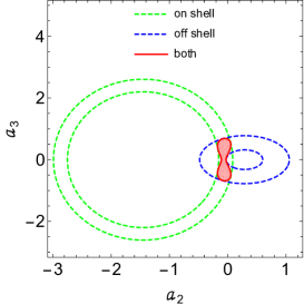
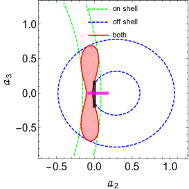
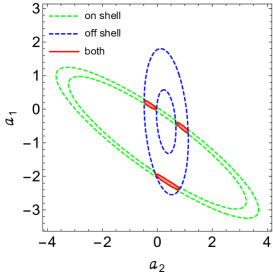
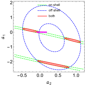
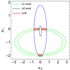
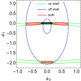
Figure 5: Two-dimensional constraints on the new physics coefficients $a_{1}$,$a_{2}$ and $a_{3}$ from $\chi^{2}$ fits. To illustrate the constraints from different energy regions, three $1\sigma$ regions (green concentric circles, blue concentric circles, and red region) from three individual $\chi^{2}$ fits (on-shell, off-shell, and both) are drawn here. CMS $2\sigma$ constraints ($95\%$ confidence level) Sirunyan:2019twz are drawn as the lines (magenta for $a_{2}$ when $a_{1}=a_{3}=0$ and grey for $a_{3}$ when $a_{1}=a_{2}=0$) in the right zoom in plots.

Fig.5 shows the two dimensional contour diagram of the anomalous couplings. There are three colored regions (green, blue, and red) in each small plot and the red areas are the final $1\sigma$ survival parameter regions from the global $\chi^{2}$ fit. In the actual two dimensional fitting procedure, we take two anomalous couplings to be free and fix the third one to be zero. Three individual $\chi^{2}$ fits are operated, constraint only from the off-region (first part in Eq. (31)), constraint from the on-shell region (second part in Eq. (31)) and both of the two. The purpose is to show how the irregular overlap red regions come from. As discussed in above sections, we have equal number of experimental data points and free parameters here and the $\chi^{2}$ fit degenerates to an equation solving problem. Survival parameter regions from either on-shell or off-shell constraint come to be concentric circles and the global fitting results are almost the overlap region between them.

In the recently updated CMS experiment Sirunyan:2019twz , it use both on-shell and off-shell data, construct kinematic discriminants, and get the limit (at 95% confidence level) of the parameters $a_{2}\subset[-0.09,0.19]$, $a_{3}\subset[-0.21,0.18]$ (there is no corresponding constraint on $a_{1}$). This experimental analysis is based on one free parameter-fitting schedule so we draw them as the line segments in the right plots of Fig. 5 (magenta for $a_{2}$ and grey for $a_{3}$). Our global fit results is roughly consistent with the CMS’s, although within a first glance the two seems have some tension(Pay attention that we draw $1\sigma$ contour while CMS’s results are the limit at 95% confidence level which corresponds to $2\sigma$ intervals in the hypothesis of Gaussian distribution). The CMS’s results seems to be more stringent than ours. This maybe caused by more kinematic information in detail they used in their analysis. Besides, we have some parameter regions with $a_{1}\sim-2$ or $a_{2}$ approaching 1. These regions show the correlations of each pairs of parameters. There is cancellation on the cross sections when the parameters coexist. In principle, the anomalous couplings should be much smaller than 1 to validate the operator expansion. Therefore, these parameter regions should be ruled out. Nevertheless, our global fit provides a complementary perspective of how the final anomalous coupling parameters contour regions are obtained from the individual on-shell/off-shell energy region constraints. These preliminary fitting results can be optimized in the case of more statistics in the future.

V conclusion and discussion

When considering the anomalous $HZZ$ couplings, we calculate the cross sections induced by these new couplings, and special attention is focused on the interference effects. In principle, there are three kinds of interference: 1. the interference between anomalous $CP$-even Higgs-mediated process and the continuum background box process $\sigma_{CP\text{-even},\text{box}}$; 2. the interference between anomalous $CP$-even Higgs-mediated process and SM Higgs-mediated process $\sigma_{CP\text{-even},\text{SM}}$; and 3. the interference between the anomalous $CP$-odd Higgs-mediated process and all other processes $\sigma_{CP\text{-odd},k}$ with $k={\text{box},\text{SM},CP\text{-even}}$. The numerical results of the integrated cross sections show that the first kind of interference can be neglected in the on-shell Higgs region but is nonnegligible in the off-shell Higgs region, the second kind of interference is important in both the on-shell and off-shell Higgs regions, and the third kind of interference has zero contribution for the total cross section in both regions.

By using the theoretical calculation together with both on-shell and off-shell Higgs experimental data, we estimate the constraints on the anomalous $HZZ$ couplings. The correlations of the different kinds of anomalous couplings are shown in contour plots, which illustrate how the anomalous contributions cancel each other out and the extra parameter regions survive when they coexist.

In this research we only use the numerical results of integrated cross sections, whereas in fact more information can be fetched from the differential cross sections (kinematic distributions). Furthermore, the $k$-factors and total efficiencies should also be estimated separately according to different sources. We leave them for our future work.

Appendix A Helicity amplitudes for the process $H\rightarrow ZZ\to e^{-}e^{+}\mu^{-}\mu^{+}$

The helicity amplitudes $\mathcal{A}_{1}$, $\mathcal{A}_{2}$ and $\mathcal{A}_{3}$ are shown separately. The common factor $f$ is defined as

$$f=-2ie^{3}\frac{1}{M_{W}\sin\theta_{W}}\frac{P_{Z}(s_{34})}{s_{34}}\frac{P_{Z}(s_{56})}{s_{56}}~{}.$$

$$\mathcal{A}_{1}^{H\rightarrow ZZ\to 2e2\mu}(3^{-}_{e^{-}},4^{+}_{e^{+}},5^{-}_{\mu^{-}},6^{+}_{\mu^{+}})=f\times l^{2}_{e}\frac{M_{W}^{2}}{\cos^{2}\theta_{W}}\langle 35\rangle[46],$$ (32)

$$\mathcal{A}_{1}^{H\rightarrow ZZ\to 2e2\mu}(3^{-}_{e^{-}},4^{+}_{e^{+}},5^{+}_{\mu^{-}},6^{-}_{\mu^{+}})=f\times l_{e}r_{e}\frac{M_{W}^{2}}{\cos^{2}\theta_{W}}\langle 36\rangle[45],$$

$$\mathcal{A}_{1}^{H\rightarrow ZZ\to 2e2\mu}(3^{+}_{e^{-}},4^{-}_{e^{+}},5^{-}_{\mu^{-}},6^{+}_{\mu^{+}})=f\times l_{e}r_{e}\frac{M_{W}^{2}}{\cos^{2}\theta_{W}}\langle 45\rangle[36],$$

$$\mathcal{A}_{1}^{H\rightarrow ZZ\to 2e2\mu}(3^{+}_{e^{-}},4^{-}_{e^{+}},5^{+}_{\mu^{-}},6^{-}_{\mu^{+}})=f\times r^{2}_{e}\frac{M_{W}^{2}}{\cos^{2}\theta_{W}}\langle 46\rangle[35]~{}.$$

$$\mathcal{A}_{2}^{H\rightarrow ZZ\to 2e2\mu}(3^{-}_{e^{-}},4^{+}_{e^{+}},5^{-}_{\mu^{-}},6^{+}_{\mu^{+}})=f\times l^{2}_{e}\times$$ (33)

$$\Big{[}2k\cdot k^{\prime}\langle 35\rangle[46]+\big{(}\langle 35\rangle[45]+\langle 36\rangle[46]\big{)}\big{(}\langle 35\rangle[36]+\langle 45\rangle[46]\big{)}\Big{]},$$

$$\mathcal{A}_{2}^{H\rightarrow ZZ\to 2e2\mu}(3^{-}_{e^{-}},4^{+}_{e^{+}},5^{+}_{\mu^{-}},6^{-}_{\mu^{+}})=f\times l_{e}r_{e}\times$$

$$\Big{[}2k\cdot k^{\prime}\langle 36\rangle[45]+\big{(}\langle 35\rangle[45]+\langle 36\rangle[46]\big{)}\big{(}\langle 36\rangle[35]+\langle 46\rangle[45]\big{)}\Big{]},$$

$$\mathcal{A}_{2}^{H\rightarrow ZZ\to 2e2\mu}(3^{+}_{e^{-}},4^{-}_{e^{+}},5^{-}_{\mu^{-}},6^{+}_{\mu^{+}})=f\times r_{e}l_{e}\times$$

$$\Big{[}2k\cdot k^{\prime}\langle 45\rangle[36]+\big{(}\langle 45\rangle[35]+\langle 46\rangle[36]\big{)}\big{(}\langle 35\rangle[36]+\langle 45\rangle[46]\big{)}\Big{]},$$

$$\mathcal{A}_{2}^{H\rightarrow ZZ\to 2e2\mu}(3^{+}_{e^{-}},4^{-}_{e^{+}},5^{+}_{\mu^{-}},6^{-}_{\mu^{+}})=f\times r^{2}_{e}\times$$

$$\Big{[}2k\cdot k^{\prime}\langle 46\rangle[35]+\big{(}\langle 45\rangle[35]+\langle 46\rangle[36]\big{)}\big{(}\langle 36\rangle[35]+\langle 46\rangle[45]\big{)}\Big{]}.$$

$$\mathcal{A}_{3}^{H\rightarrow ZZ\to 2e2\mu}(3^{-}_{e^{-}},4^{+}_{e^{+}},5^{-}_{\mu^{-}},6^{+}_{\mu^{+}})=f\times l^{2}_{e}\times(-i)\times$$ (34)

$$\Big{[}2\big{(}k\cdot k^{\prime}+\langle 46\rangle[46]\big{)}\langle 35\rangle[46]+\langle 35\rangle[45]\big{(}\langle 35\rangle[36]+\langle 45\rangle[46]\big{)}$$

$$+\langle 36\rangle[46]\big{(}\langle 35\rangle[36]-\langle 45\rangle[46]\big{)}\Big{]}~{},$$

$$\mathcal{A}_{3}^{H\rightarrow ZZ\to 2e2\mu}(3^{-}_{e^{-}},4^{+}_{e^{+}},5^{+}_{\mu^{-}},6^{-}_{\mu^{+}})=f\times l_{e}r_{e}\times(-i)\times$$

$$\Big{[}2\big{(}k\cdot k^{\prime}+\langle 45\rangle[45]\big{)}\langle 36\rangle[45]+\langle 36\rangle[46]\big{(}\langle 36\rangle[35]+\langle 46\rangle[45]\big{)}$$

$$+\langle 35\rangle[45]\big{(}\langle 36\rangle[35]-\langle 46\rangle[45]\big{)}\Big{]},$$

$$\mathcal{A}_{3}^{H\rightarrow ZZ\to 2e2\mu}(3^{+}_{e^{-}},4^{-}_{e^{+}},5^{-}_{\mu^{-}},6^{+}_{\mu^{+}})=f\times r_{e}l_{e}\times(-i)\times$$

$$\Big{[}2\big{(}k\cdot k^{\prime}+\langle 36\rangle[36]\big{)}\langle 45\rangle[36]+\langle 45\rangle[35]\big{(}\langle 45\rangle[46]+\langle 35\rangle[36]\big{)}$$

$$+\langle 46\rangle[36]\big{(}\langle 45\rangle[46]-\langle 35\rangle[36]\big{)}\Big{]},$$

$$\mathcal{A}_{3}^{H\rightarrow ZZ\to 2e2\mu}(3^{+}_{e^{-}},4^{-}_{e^{+}},5^{+}_{\mu^{-}},6^{-}_{\mu^{+}})=f\times r^{2}_{e}\times(-i)\times$$

$$\Big{[}2\big{(}k\cdot k^{\prime}+\langle 35\rangle[35]\big{)}\langle 46\rangle[35]+\langle 46\rangle[36]\big{(}\langle 46\rangle[45]+\langle 36\rangle[35]\big{)}$$

$$+\langle 45\rangle[35]\big{(}\langle 46\rangle[45]-\langle 36\rangle[35]\big{)}\Big{]}.$$

Appendix B The cross sections at $\sqrt{s}=8$ TeV

8 TeV, $m_{2e2\mu}<130\rm~{}GeV$, on-shell
$\sigma_{k,l}$(fb)		box	Higgs-med.
			SM	$CP$-even	$CP$-odd
box		0.011	0	0	0
Higgs-med.	SM	0	0.232	0.257	0
	$CP$-even	0	0.257	0.093	0
	$CP$-odd	0	0	0	0.035

8 TeV , $m_{2e2\mu}>220\rm~{}GeV$, off-shell
$\sigma_{k,l}$(fb)		box	Higgs-med.
			SM	$CP$-even	$CP$-odd
box		0.479	-0.056	-0.198	0
Higgs-med.	SM	-0.056	0.031	0.047	0
	$CP$-even	-0.198	0.047	0.228	0
	$CP$-odd	0	0	0	0.219

Table 3: Cross sections of $gg\to 2e2\mu$ process in proton-proton collision at $\sqrt{s}=8$ TeV with $a_{1}=0,a_{2}=a_{3}=1$ in Eq. (6).

8 TeV , $m_{4e/4\mu}<130\rm~{}GeV$, on-shell
$\sigma_{k,l}$(fb)		box	Higgs-med.
			SM	$CP$-even	$CP$-odd
box		0.021	0	0	0
Higgs-med.	SM	0	0.248	0.261	0
	$CP$-even	0	0.261	0.086	0
	$CP$-odd	0	0	0	0.028

8 TeV , $m_{4e/4\mu}>220\rm~{}GeV$, off-shell
$\sigma_{k,l}$(fb)		box	Higgs-med.
			SM	$CP$-even	$CP$-odd
box		0.485	-0.056	-0.199	0
Higgs-med.	SM	-0.056	0.031	0.047	0
	$CP$-even	-0.199	0.047	0.229	0
	$CP$-odd	0	0	0	0.215

Table 4: The cross sections of $gg\to 4e/4\mu$ processes in proton-proton collision at center-of-mass energy $\sqrt{s}=8$ TeV with $a_{1}=0,a_{2}=a_{3}=1$ in Eq. (6).

References

- (1) CMS Collaboration, S. Chatrchyan et al., “Observation of a new boson at a mass of 125 GeV with the CMS experiment at the LHC,” Phys. Lett. B716 (2012) 30–61, arXiv:1207.7235 [hep-ex].
- (2) ATLAS Collaboration, G. Aad et al., “Observation of a new particle in the search for the Standard Model Higgs boson with the ATLAS detector at the LHC,” Phys. Lett. B716 (2012) 1–29, arXiv:1207.7214 [hep-ex].
- (3) CMS Collaboration, A. M. Sirunyan et al., “Combined measurements of Higgs boson couplings in proton-proton collisions at 13 TeV,” Submitted to: Eur. Phys. J. (2018) , arXiv:1809.10733 [hep-ex].
- (4) CMS Collaboration, J. Tao, “Measurements of the 125 GeV Higgs boson at CMS,” in 21st High-Energy Physics International Conference in Quantum Chromodynamics (QCD 18) Montpellier, France, July 2-6, 2018. 2018. arXiv:1810.00256 [hep-ex].
- (5) ATLAS, CMS Collaboration, A.-M. Magnan, “The Higgs boson at the LHC: standard model Higgs properties and beyond standard model searches,” PoS ALPS2018 (2018) 013.
- (6) Y. Gao, A. V. Gritsan, Z. Guo, K. Melnikov, M. Schulze, and N. V. Tran, “Spin determination of single-produced resonances at hadron colliders,” Phys. Rev. D81 (2010) 075022, arXiv:1001.3396 [hep-ph].
- (7) S. Bolognesi, Y. Gao, A. V. Gritsan, K. Melnikov, M. Schulze, N. V. Tran, and A. Whitbeck, “On the spin and parity of a single-produced resonance at the LHC,” Phys. Rev. D86 (2012) 095031, arXiv:1208.4018 [hep-ph].
- (8) I. Anderson et al., “Constraining anomalous HVV interactions at proton and lepton colliders,” Phys. Rev. D89 (2014) no. 3, 035007, arXiv:1309.4819 [hep-ph].
- (9) Y. Chen, N. Tran, and R. Vega-Morales, “Scrutinizing the Higgs Signal and Background in the Golden Channel,” JHEP 01 (2013) 182, arXiv:1211.1959 [hep-ph].
- (10) Y. Chen and R. Vega-Morales, “Extracting Effective Higgs Couplings in the Golden Channel,” JHEP 04 (2014) 057, arXiv:1310.2893 [hep-ph].
- (11) Y. Chen, E. Di Marco, J. Lykken, M. Spiropulu, R. Vega-Morales, and S. Xie, “8D likelihood effective Higgs couplings extraction framework in ,” JHEP 01 (2015) 125, arXiv:1401.2077 [hep-ex].
- (12) Y. Chen, E. Di Marco, J. Lykken, M. Spiropulu, R. Vega-Morales, and S. Xie, “Technical Note for 8D Likelihood Effective Higgs Couplings Extraction Framework in the Golden Channel,” arXiv:1410.4817 [hep-ph].
- (13) C. A. Nelson, “Correlation Between Decay Planes in Higgs Boson Decays Into Pair (Into Pair),” Phys. Rev. D37 (1988) 1220.
- (14) A. Soni and R. M. Xu, “Probing CP violation via Higgs decays to four leptons,” Phys. Rev. D48 (1993) 5259–5263, arXiv:hep-ph/9301225 [hep-ph].
- (15) D. Chang, W.-Y. Keung, and I. Phillips, “CP odd correlation in the decay of neutral Higgs boson into Z Z, W+ W-, or t anti-t,” Phys. Rev. D48 (1993) 3225–3234, arXiv:hep-ph/9303226 [hep-ph].
- (16) T. Arens and L. M. Sehgal, “Energy spectra and energy correlations in the decay H Z Z mu+ mu- mu+ mu-,” Z. Phys. C66 (1995) 89–94, arXiv:hep-ph/9409396 [hep-ph].
- (17) S. Y. Choi, D. J. Miller, M. M. Muhlleitner, and P. M. Zerwas, “Identifying the Higgs spin and parity in decays to Z pairs,” Phys. Lett. B553 (2003) 61–71, arXiv:hep-ph/0210077 [hep-ph].
- (18) C. P. Buszello, I. Fleck, P. Marquard, and J. J. van der Bij, “Prospective analysis of spin- and CP-sensitive variables in HZ Z l(1)+ l(1)- l(2)+ l(2)- at the LHC,” Eur. Phys. J. C32 (2004) 209–219, arXiv:hep-ph/0212396 [hep-ph].
- (19) R. M. Godbole, D. J. Miller, and M. M. Muhlleitner, “Aspects of CP violation in the H ZZ coupling at the LHC,” JHEP 12 (2007) 031, arXiv:0708.0458 [hep-ph].
- (20) V. A. Kovalchuk, “Model-independent analysis of CP violation effects in decays of the Higgs boson into a pair of the W and Z bosons,” J. Exp. Theor. Phys. 107 (2008) 774–786.
- (21) Q.-H. Cao, C. B. Jackson, W.-Y. Keung, I. Low, and J. Shu, “The Higgs Mechanism and Loop-induced Decays of a Scalar into Two Z Bosons,” Phys. Rev. D81 (2010) 015010, arXiv:0911.3398 [hep-ph].
- (22) A. De Rujula, J. Lykken, M. Pierini, C. Rogan, and M. Spiropulu, “Higgs look-alikes at the LHC,” Phys. Rev. D82 (2010) 013003, arXiv:1001.5300 [hep-ph].
- (23) J. S. Gainer, K. Kumar, I. Low, and R. Vega-Morales, “Improving the sensitivity of Higgs boson searches in the golden channel,” JHEP 11 (2011) 027, arXiv:1108.2274 [hep-ph].
- (24) B. Coleppa, K. Kumar, and H. E. Logan, “Can the 126 GeV boson be a pseudoscalar?,” Phys. Rev. D86 (2012) 075022, arXiv:1208.2692 [hep-ph].
- (25) D. Stolarski and R. Vega-Morales, “Directly Measuring the Tensor Structure of the Scalar Coupling to Gauge Bosons,” Phys. Rev. D86 (2012) 117504, arXiv:1208.4840 [hep-ph].
- (26) R. Boughezal, T. J. LeCompte, and F. Petriello, “Single-variable asymmetries for measuring the ‘Higgs’ boson spin and CP properties,” arXiv:1208.4311 [hep-ph].
- (27) P. Avery et al., “Precision studies of the Higgs boson decay channel with MEKD,” Phys. Rev. D87 (2013) no. 5, 055006, arXiv:1210.0896 [hep-ph].
- (28) J. M. Campbell, W. T. Giele, and C. Williams, “Extending the Matrix Element Method to Next-to-Leading Order,” in Proceedings, 47th Rencontres de Moriond on QCD and High Energy Interactions: La Thuile, France, March 10-17, 2012, pp. 319–322. 2012. arXiv:1205.3434 [hep-ph]. http://lss.fnal.gov/archive/2012/conf/fermilab-conf-12-176-t.pdf.
- (29) J. M. Campbell, W. T. Giele, and C. Williams, “The Matrix Element Method at Next-to-Leading Order,” JHEP 11 (2012) 043, arXiv:1204.4424 [hep-ph].
- (30) A. Menon, T. Modak, D. Sahoo, R. Sinha, and H.-Y. Cheng, “Inferring the nature of the boson at 125-126 GeV,” Phys. Rev. D89 (2014) no. 9, 095021, arXiv:1301.5404 [hep-ph].
- (31) Y. Sun, X.-F. Wang, and D.-N. Gao, “CP mixed property of the Higgs-like particle in the decay channel ,” Int. J. Mod. Phys. A29 (2014) 1450086, arXiv:1309.4171 [hep-ph].
- (32) J. S. Gainer, J. Lykken, K. T. Matchev, S. Mrenna, and M. Park, “Geolocating the Higgs Boson Candidate at the LHC,” Phys. Rev. Lett. 111 (2013) 041801, arXiv:1304.4936 [hep-ph].
- (33) G. Buchalla, O. Cata, and G. D’Ambrosio, “Nonstandard Higgs couplings from angular distributions in ,” Eur. Phys. J. C74 (2014) no. 3, 2798, arXiv:1310.2574 [hep-ph].
- (34) M. Chen, T. Cheng, J. S. Gainer, A. Korytov, K. T. Matchev, P. Milenovic, G. Mitselmakher, M. Park, A. Rinkevicius, and M. Snowball, “The role of interference in unraveling the ZZ-couplings of the newly discovered boson at the LHC,” Phys. Rev. D89 (2014) no. 3, 034002, arXiv:1310.1397 [hep-ph].
- (35) N. Kauer and G. Passarino, “Inadequacy of zero-width approximation for a light Higgs boson signal,” JHEP 08 (2012) 116, arXiv:1206.4803 [hep-ph].
- (36) M. Beneke, D. Boito, and Y.-M. Wang, “Anomalous Higgs couplings in angular asymmetries of and e+ e,” JHEP 11 (2014) 028, arXiv:1406.1361 [hep-ph].
- (37) A. Falkowski and R. Vega-Morales, “Exotic Higgs decays in the golden channel,” JHEP 12 (2014) 037, arXiv:1405.1095 [hep-ph].
- (38) T. Modak, D. Sahoo, R. Sinha, H.-Y. Cheng, and T.-C. Yuan, “Disentangling the Spin-Parity of a Resonance via the Gold-Plated Decay Mode,” Chin. Phys. C40 (2016) no. 3, 033002, arXiv:1408.5665 [hep-ph].
- (39) M. Gonzalez-Alonso and G. Isidori, “The spectrum at low : Standard Model vs. light New Physics,” Phys. Lett. B733 (2014) 359–365, arXiv:1403.2648 [hep-ph].
- (40) N. Belyaev, R. Konoplich, L. E. Pedersen, and K. Prokofiev, “Angular asymmetries as a probe for anomalous contributions to HZZ vertex at the LHC,” Phys. Rev. D91 (2015) no. 11, 115014, arXiv:1502.03045 [hep-ph].
- (41) J. S. Gainer et al., “Adding pseudo-observables to the four-lepton experimentalist’s toolbox,” JHEP 10 (2018) 073, arXiv:1808.00965 [hep-ph].
- (42) CMS Collaboration, S. Chatrchyan et al., “Study of the Mass and Spin-Parity of the Higgs Boson Candidate Via Its Decays to Z Boson Pairs,” Phys. Rev. Lett. 110 (2013) no. 8, 081803, arXiv:1212.6639 [hep-ex].
- (43) CMS Collaboration, V. Khachatryan et al., “Constraints on the spin-parity and anomalous HVV couplings of the Higgs boson in proton collisions at 7 and 8 TeV,” Phys. Rev. D92 (2015) no. 1, 012004, arXiv:1411.3441 [hep-ex].
- (44) CMS Collaboration, V. Khachatryan et al., “Constraints on the Higgs boson width from off-shell production and decay to Z-boson pairs,” Phys. Lett. B736 (2014) 64–85, arXiv:1405.3455 [hep-ex].
- (45) LHC Higgs Cross Section Working Group Collaboration, D. de Florian et al., “Handbook of LHC Higgs Cross Sections: 4. Deciphering the Nature of the Higgs Sector,” arXiv:1610.07922 [hep-ph].
- (46) CMS Collaboration, A. M. Sirunyan et al., “Constraints on anomalous Higgs boson couplings using production and decay information in the four-lepton final state,” Phys. Lett. B775 (2017) 1–24, arXiv:1707.00541 [hep-ex].
- (47) CMS Collaboration, A. M. Sirunyan et al., “Measurements of the Higgs boson width and anomalous couplings from on-shell and off-shell production in the four-lepton final state,” Phys. Rev. D 99 (2019) no. 11, 112003, arXiv:1901.00174 [hep-ex].
- (48) ATLAS Collaboration, G. Aad et al., “Constraints on the off-shell Higgs boson signal strength in the high-mass and final states with the ATLAS detector,” Eur. Phys. J. C75 (2015) no. 7, 335, arXiv:1503.01060 [hep-ex].
- (49) ATLAS Collaboration, M. Aaboud et al., “Measurement of the Higgs boson mass in the and channels with TeV collisions using the ATLAS detector,” Phys. Lett. B784 (2018) 345–366, arXiv:1806.00242 [hep-ex].
- (50) ATLAS Collaboration, M. Aaboud et al., “Constraints on off-shell Higgs boson production and the Higgs boson total width in and final states with the ATLAS detector,” Phys. Lett. B786 (2018) 223–244, arXiv:1808.01191 [hep-ex].
- (51) J. M. Campbell, R. K. Ellis, and C. Williams, “Bounding the Higgs width at the LHC using full analytic results for ,” JHEP 04 (2014) 060, arXiv:1311.3589 [hep-ph].
- (52) J. M. Campbell, R. K. Ellis, and C. Williams, “Gluon-Gluon Contributions to W+ W- Production and Higgs Interference Effects,” JHEP 10 (2011) 005, arXiv:1107.5569 [hep-ph].
- (53) J. M. Campbell, R. K. Ellis, and C. Williams, “Bounding the Higgs Width at the LHC,” PoS LL2014 (2014) 008, arXiv:1408.1723 [hep-ph].
- (54) W. Buchmuller and D. Wyler, “Effective Lagrangian Analysis of New Interactions and Flavor Conservation,” Nucl. Phys. B268 (1986) 621–653.
- (55) B. Grzadkowski, M. Iskrzynski, M. Misiak, and J. Rosiek, “Dimension-Six Terms in the Standard Model Lagrangian,” JHEP 10 (2010) 085, arXiv:1008.4884 [hep-ph].
- (56) T. Barklow, K. Fujii, S. Jung, M. E. Peskin, and J. Tian, “Model-Independent Determination of the Triple Higgs Coupling at e+e- Colliders,” Phys. Rev. D 97 (2018) no. 5, 053004, arXiv:1708.09079 [hep-ph].
- (57) J. Cohen, S. Bar-Shalom, and G. Eilam, “Contact Interactions in Higgs-Vector Boson Associated Production at the ILC,” Phys. Rev. D 94 (2016) no. 3, 035030, arXiv:1602.01698 [hep-ph].
- (58) L. J. Dixon, “Calculating scattering amplitudes efficiently,” in QCD and beyond. Proceedings, Theoretical Advanced Study Institute in Elementary Particle Physics, TASI-95, Boulder, USA, June 4-30, 1995, pp. 539–584. 1996. arXiv:hep-ph/9601359 [hep-ph]. http://www-public.slac.stanford.edu/sciDoc/docMeta.aspx?slacPubNumber=SLAC-PUB-7106.
- (59) G. Passarino and M. J. G. Veltman, “One Loop Corrections for e+ e- Annihilation Into mu+ mu- in the Weinberg Model,” Nucl. Phys. B160 (1979) 151–207.
- (60) X. Chen, G. Li, and X. Wan, “Probe CP violation in through forward-backward asymmetry,” Phys. Rev. D96 (2017) no. 5, 055023, arXiv:1705.01254 [hep-ph].
- (61) T. Binoth, N. Kauer, and P. Mertsch, “Gluon-induced QCD corrections to pp ZZ l anti-l l-prime anti-l-prime,” in Proceedings, 16th International Workshop on Deep Inelastic Scattering and Related Subjects (DIS 2008): London, UK, April 7-11, 2008, p. 142. 2008. arXiv:0807.0024 [hep-ph].
- (62) J. M. Campbell, R. K. Ellis, and W. T. Giele, “A Multi-Threaded Version of MCFM,” Eur. Phys. J. C75 (2015) no. 6, 246, arXiv:1503.06182 [physics.comp-ph].
- (63) R. Boughezal, J. M. Campbell, R. K. Ellis, C. Focke, W. Giele, X. Liu, F. Petriello, and C. Williams, “Color singlet production at NNLO in MCFM,” Eur. Phys. J. C77 (2017) no. 1, 7, arXiv:1605.08011 [hep-ph].
- (64) A. D. Martin, W. J. Stirling, R. S. Thorne, and G. Watt, “Parton distributions for the LHC,” Eur. Phys. J. C63 (2009) 189–285, arXiv:0901.0002 [hep-ph].
- (65) CMS Collaboration Collaboration, C. Collaboration, “Properties of the Higgs-like boson in the decay H to ZZ to 4l in pp collisions at sqrt s =7 and 8 TeV,” Tech. Rep. CMS-PAS-HIG-13-002, CERN, Geneva, 2013. http://cds.cern.ch/record/1523767.
- (66) F. Caola, K. Melnikov, R. Rontsch, and L. Tancredi, “QCD corrections to ZZ production in gluon fusion at the LHC,” Phys. Rev. D92 (2015) no. 9, 094028, arXiv:1509.06734 [hep-ph].
- (67) K. Melnikov and M. Dowling, “Production of two Z-bosons in gluon fusion in the heavy top quark approximation,” Phys. Lett. B744 (2015) 43–47, arXiv:1503.01274 [hep-ph].
- (68) J. M. Campbell, R. K. Ellis, M. Czakon, and S. Kirchner, “Two loop correction to interference in ,” JHEP 08 (2016) 011, arXiv:1605.01380 [hep-ph].
- (69) F. Caola, M. Dowling, K. Melnikov, R. Rontsch, and L. Tancredi, “QCD corrections to vector boson pair production in gluon fusion including interference effects with off-shell Higgs at the LHC,” JHEP 07 (2016) 087, arXiv:1605.04610 [hep-ph].
- (70) CMS Collaboration Collaboration, C. Collaboration, “Measurements of properties of the Higgs boson in the four-lepton final state in proton-proton collisions at ,” Tech. Rep. CMS-PAS-HIG-19-001, CERN, Geneva, 2019. http://cds.cern.ch/record/2668684.