Theoretical predictions on polarization asymmetry for Drell-Yan process with spin-one deuteron
and tensor-polarized structure function $\mathbold{b_{1}}$

Abstract:

We report recent theoretical progress on a polarization asymmetry in the proton-deuteron Drell-Yan process with a polarized-deuteron target and the tensor-polarized structure function $b_{1}$. Experimental measurements are possible at JLab for $b_{1}$ and at Fermilab for the Drell-Yan process. First, we show a theoretical estimate for the proton-deuteron Drell-Yan asymmetry in the Fermilab-E1039 experiment. We evolved tensor-polarized parton distribution functions, which explain existing HERMES $b_{1}$ data, at $Q^{2}=2.5$ GeV² to the $Q^{2}$ range of the Fermilab Drell-Yan measurements. Then, we predicted that the asymmetry is of the order of a few percent. The Drell-Yan experiment has an advantage to probe the tensor-polarized antiquark distributions, which were suggested by the HERMES experiment as a finite sum for $b_{1}$ ($\int dxb_{1}(x)\neq 0$). Second, we predicted $b_{1}$ for the JLab experiment by the standard convolution model of the deuteron. Our theoretical $b_{1}$ structure function seems to be much different from the HERMES data. Furthermore, a significant distribution exists at very large $x$ ($>1$) beyond the kinematical limit $x_{max}=1$ for the proton. Because the standard deuteron-model estimate is much different from the HERMES data, there could be an interesting development as a new hadron-physics field if future JLab data will be much different from our conventional prediction.

1 Introduction

Origin of nucleon spin has been investigated especially from the late 1980’s, and major properties became clear. On the other hand, spin structure of spin-1 hadrons, such as the deuteron, has not been seriously investigated at high energies, although electromagnetic properties were studied at low energies such as electric quadrupole form factors. It is possible to probe new spin structure functions [1, 2, 3] which do not exist in the nucleon. There was a HERMES measurement for the deuteron [4]; however, its errors are still large. There is an approved experiment E12-13-011 at JLab (Thomas Jefferson National Accelerator Facility) to measure a tensor-polarized structure function and it will start soon [5]. Furthermore, a polarized proton-deuteron Drell-Yan experiment is under consideration in the Fermilab-E1039 experiment [6]. Spin physics of spin-1 deuteron could become one of active hadron-physics fields to understand it in terms of quark and gluon degrees of freedom in the near future.

Due to the spin-one nature, the deuteron has additional structure functions in comparison with proton ones, and they can be investigated in the deep inelastic scattering (DIS) of a charged lepton with a polarized deuteron. The hadron tensor is defined for the spin-1 deuteron as [2, 3]

$$W_{\mu\nu}^{\lambda_{f}\lambda_{i}}= \frac{1}{4\pi M}\int d^{4}xe^{iqx}\left\langle p\,\lambda_{f}|J_{\mu}(x)J_{\nu}(0)|p\,\lambda_{i}\right\rangle$$

$$= -F_{1}\hat{g}_{\mu\nu}+\frac{F_{2}}{M\nu}\hat{p}_{\mu}\hat{p}_{\nu}+\frac{ig_{1}}{\nu}\epsilon_{\mu\nu\lambda\sigma}q^{\lambda}s^{\sigma}+\frac{ig_{2}}{M\nu^{2}}\epsilon_{\mu\nu\lambda\sigma}q^{\lambda}(p\cdot qs^{\sigma}-s\cdot qp^{\sigma})$$

$$-b_{1}r_{\mu\nu}+\frac{1}{6}b_{2}(s_{\mu\nu}+t_{\mu\nu}+u_{\mu\nu})+\frac{1}{2}b_{3}(s_{\mu\nu}-u_{\mu\nu})+\frac{1}{2}b_{4}(s_{\mu\nu}-t_{\mu\nu}),$$ (1)

where $p$ is the momentum of the deuteron, $q$ is the momentum of the virtual photon, and $\lambda_{i}$ and $\lambda_{f}$ indicate initial and final spin states of the deuteron, respectively. The notations $\hat{g}_{\mu\nu}$ and $\hat{p}_{\mu}$ are defined as $\hat{g}_{\mu\nu}\equiv g_{\mu\nu}-{q_{\mu}q_{\nu}}/{q^{2}}$ and $\hat{p}_{\mu}\equiv p_{\mu}-({p\cdot q}/{q^{2}})\,q_{\mu}$, $s^{\mu}$ is the spin vector of the deuteron, and one can find definitions of other kinematical variables in Refs. [2, 3]. In Eq. (1), there are 8 structure functions in total. The structure functions $F_{1}$, $F_{2}$, $g_{1}$ and $g_{2}$ appear in the hadron tensor of the proton, whereas the structure functions $b_{1}$, $b_{2}$, $b_{3}$ and $b_{4}$ are the new ones for the deuteron. The leading-twist structure functions are $b_{1}$ and $b_{2}$, and they are related with each other by the Callan-Gross like relation $b_{2}=2xb_{1}$. The functions $b_{3}$ and $b_{4}$ are higher-twist ones.

As the first step, we may investigate the leading-twist function $b_{1}$ among the tensor-polarized structure functions $b_{1-4}$. The function $b_{1}$ will clarify the tensor structure of the deuteron in terms of quarks and gluons, and it is expressed by the tensor-polarized parton distribution functions (PDFs) $\delta_{T}q_{i}$ as

$$b_{1}(x)=\frac{1}{2}\sum_{i}e_{i}^{2}\left[\delta_{T}q_{i}(x)+\delta_{T}\bar{q}_{i}(x)\right],\ \ \delta_{T}q_{i}(x)\equiv q^{0}_{i}(x)-\frac{q_{i}^{+1}(x)+q_{i}^{-1}(x)}{2},$$ (2)

where the index $i$ is the quark flavor, the superscripts (0, $\pm$) indicate the deuteron spin state, and the scale-$Q^{2}$ dependence is abbreviated for simplicity. There is an interesting sum rule of $b_{1}$ [7]:

$$\int dx\,b_{1}(x)=-\lim_{t\to 0}\,\frac{5}{24}\,t\,F_{Q}(t)+\frac{1}{9}\!\int\!dx\left[4\delta_{T}\bar{u}(x)+4\delta_{T}\bar{d}(x)+\delta_{T}\bar{s}(x)\right],$$ (3)

where $F_{Q}(t)$ is the electric quadrupole form factor. Because the first term vanishes, the nonzero integral of $b_{1}$ indicates the existence of finite tensor-polarized antiquark distributions.

The first measurement of $b_{1}$ was conducted by the HERMES collaboration [4], and the values of $b_{1}$ are of the order of $10^{-2}$. However, theoretical predictions of $b_{1}$ are much smaller than the experimental measurements [8, 9] as we show later in Sec. 3.3 by conventional convolution models. The HERMES collaboration also reported the integrals of $b_{1}$ as

$$\!\!\!\int_{0.002}^{0.85}\!dx\,b_{1}(x) =\left[0.35\pm 0.10(\text{stat})\pm 0.18(\text{sys})\right]\times 10^{-2}\ \ \text{(in the range of $Q^{2}>1$ GeV${}^{2}$)},$$ (4)

and it was $[1.05\pm 0.34(\text{stat})\pm 0.35(\text{sys})]\times 10^{-2}$ in the whole measured range. These HERMES measurements seem to indicate the existence of finite tensor-polarized antiquark distributions according to Eq. (3). However, such tensor polarization in antiquarks may not be easily understood theoretically in simple deuteron models. In the near future, $b_{1}$ will be measured by the experiment E12-13-011 at JLab, and it could clarify the tensor structure in terms of quark and gluon degrees of freedom. However, the antiquark distributions can be measured more directly by the Drell-Yan process as discussed in the next section.

2 Theoretical estimate on tensor-polarization asymmetry in proton-deuteron Drell-Yan process

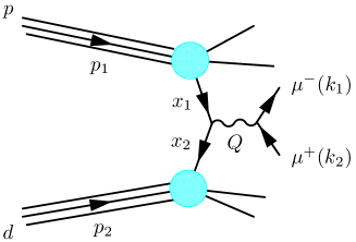
Figure 1: Proton-deuteron Drell-Yan process.

The tensor structure of the deuteron can be investigated by the proton-deuteron Drell-Yan process, which is possible at Fermilab. There is a significant advantage in probing the tensor-polarized antiquark distributions by the Drell-Yan process illustrated in Fig. 1. At Fermilab, the beam is unpolarized 120 GeV proton provided by the Main Injector and the deuteron target is tensor polarized. The momentum fractions carried by the quark and antiquark are denoted as $x_{1}$ and $x_{2}$, and the scale is given by $Q^{2}=x_{1}x_{2}s$ with the center-of-mass-energy squared $s=(p_{1}+p_{2})^{2}$.

The hadron tensor of the Drell-Yan process is complicated than that of DIS since there are more structure functions involved [10]. Among spin asymmetries, the tensor-polarization asymmetry $A_{Q}$ provides information of the tensor-polarized PDFs, and it is defined as

$$A_{Q}=\frac{1}{\left\langle\sigma\right\rangle}\left[\sigma(\bullet,0)-\frac{\sigma(\bullet,+1)+\sigma(\bullet,-1)}{2}\right],$$ (5)

where $\bullet$ represents unpolarized proton beam and the deuteron spin states are denoted as $\pm$ and $0$. The spin asymmetry $A_{Q}$ indicates the difference of the cross section with different deuteron spin states. In the parton model, $A_{Q}$ can be expressed by the tensor-polarized PDFs as [10]

$$A_{Q}=\frac{\sum_{i}e_{i}^{2}\left[q_{i}(x_{1})\delta_{T}\bar{q}_{i}(x_{2})+\bar{q}_{i}(x_{1})\delta_{T}q_{i}(x_{2})\right]}{\sum_{i}e_{i}^{2}\left[q_{i}(x_{1})\bar{q}_{i}(x_{2})+\bar{q}_{i}(x_{1})q_{i}(x_{2})\right]},$$ (6)

where the scale $Q^{2}$ is abbreviated. If $x_{F}=x_{1}-x_{2}$ is large enough, the contribution of $\bar{q}_{i}(x_{1})\delta_{T}q_{i}(x_{2})$ can be neglected in comparison with $q_{i}(x_{1})\delta_{T}\bar{q}_{i}(x_{2})$, so it is possible to probe the tensor-polarized antiquark distributions $\delta_{T}\bar{q}_{i}(x)$ by using the Drell-Yan process.

In order to predict the spin asymmetry in the Drell-Yan process at Fermilab, the tensor-polarized distributions $\delta_{T}q_{i}(x,Q^{2})$ are needed. Here, we adopt the parameterizations of $\delta_{T}q_{i}(x,Q^{2}_{0})$ in Ref. [11], where there are two sets of tensor-polarized distributions $\delta_{T}q_{i}(x,Q^{2}_{0})$ based on the analysis of HERMES data at the average scale $Q^{2}_{0}=2.5$ GeV². In the set-1 analysis, there are no tensor-polarized antiquark distributions at the initial scale $Q^{2}_{0}=2.5$ GeV²; however, finite tensor-polarized antiquark distributions are allowed in the set-2 analysis. With $\delta_{T}q_{i}(x,Q^{2}_{0})$ at the initial scale, one can obtain the tensor-polarized distributions at lager $Q^{2}$ by using DGLAP (Dokshitzer-Gribov-Lipatov-Altarelli-Parisi) evolution equations [2, 12].

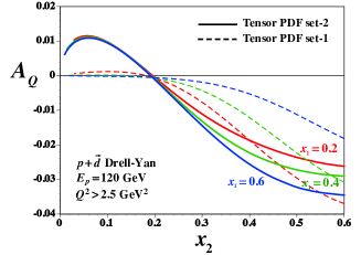
Figure 2: Spin asymmetries $A_{Q}$ at $x_{1}=0.2$, $x_{1}=0.4$ and $x_{1}=0.6$ by set 1 and 2 [13].

In Fig. 2, the spin asymmetries $A_{Q}$ are shown for the Drell-Yan experiment at Fermilab, and the momentum fraction $x_{1}$ is fixed as $x_{1}=0.2$, $x_{1}=0.4$ and $x_{1}=0.6$ in both set 1 and set 2 [13]. The spin asymmetries are not large, and they are typically of order of a few percent. The spin asymmetries of set 1 and set 2 are very different at the small $x_{2}$, since the term $q_{i}(x_{1})\delta_{T}\bar{q}_{i}(x_{2})$ is dominant in this region (large $x_{F}=x_{1}-x_{2}$) and $\delta_{T}\bar{q}_{i}(x,Q^{2}_{0})=0$ in the set 1. Because the set-2 analysis provides a better description of the HERMES measurements, the spin asymmetries of the set 2 should be more reliable than those of the set 1. In future, the spin asymmetry $A_{Q}$ could be measured by the Fermilab-E1039 (SpinQuest) collaboration in the Drell-Yan process with tensor-polarized deuteron target at Fermilab, and our theoretical predictions provide baseline for planning the experimental measurement.

3 Standard convolution model prediction for $\mathbold{b_{1}}$

A convolution formalism has been used for describing nuclear structure functions at medium and large $x$ ($x>0.2$) as a standard description to explain nuclear modifications in terms of nuclear binding and nucleon Fermi motion. A nuclear structure function is expressed by the nucleonic structure function convoluted with a spectral function which indicates a nucleon momentum distribution in a nucleus. We use this description to calculate $b_{1}$ for the deuteron. Specifically, we employ two convolution models [9] for calculating $b_{1}$ with D-state admixture in the deuteron. One is a basic convolution description, and the other is a virtual nucleon approximation which includes higher-twist contributions.

3.1 Basic convolution description (Theory 1)

In a basic convolution model for nuclear structure functions, the nuclear tensor $W_{\mu\nu}^{A}$ is given by the nucleonic one $W_{\mu\nu}$ convoluted with the nucleon’s momentum distribution expressed by the spectral function $S(p)$ as

$$\!\!\!\!W_{\mu\nu}^{A}(P_{A},q)=\int d^{4}p\,S(p)\,W_{\mu\nu}(p,q),\ \ \ S(p)=\frac{1}{A}\sum_{i}|\phi_{i}(\vec{p}\,)|^{2}\delta\bigg{(}p^{0}-M_{A}+\sqrt{M_{A-i}^{\ 2}+\vec{p}^{\ 2}}\,\bigg{)}.$$ (7)

Here, $p$ and $P_{A}$ are momenta for the nucleon and nucleus, and $\phi_{i}(\vec{p}\,)$ is the momentum-space wave function with the nucleon index $i$. This description has been successful in explaining gross features of nuclear modifications at medium and large $x$ ($x>0.2$). Physics mechanisms are contained in the spectral function as nuclear binding, Fermi motion, and short-range correlations.

For extracting the structure function $b_{1}$ from the deuteron tensor $W_{\mu\nu}^{D}(p_{{}_{D}},q)$, helicity amplitudes are defined by the photon polarization vector $\varepsilon_{h}^{\mu}$ as $A_{hH,hH}(x,Q^{2})=\varepsilon_{h}^{*\mu}\varepsilon_{h}^{\nu}\,W_{\mu\nu}^{D}(p_{{}_{D}},q)$ [2] and in the same way as $\hat{A}_{hs,hs}(x,Q^{2})$ for the nucleon. In the Bjorken scaling limit, the structure function $b_{1}$ of the deuteron and $F_{1}$ of the nucleon are expressed by the helicity amplitudes as [2, 14]

$$b_{1}=A_{+0,+0}-\frac{A_{++,++}+A_{+-,+-}}{2},\ \ \ F_{1}^{N}=\frac{A_{+\uparrow,+\uparrow}+A_{+\downarrow,+\downarrow}}{2}.$$ (8)

From these relations, the deuteron $b_{1}$ is expressed by the convolution integral with the unpolarized structure function $F_{1}^{N}$ for the nucleon as

$$b_{1}(x,Q^{2})=\int\frac{dy}{y}\,\delta_{T}f(y)\,F_{1}^{N}(x/y,Q^{2}),\ \ \ \delta_{T}f(y)\equiv f^{0}(y)-\frac{f^{+}(y)+f^{-}(y)}{2},$$ (9)

where $b_{1}$ is defined by the one per nucleon. The polarized structure function $b_{1}$ is given by “unpolarized” parton distributions in the tensor-polarized deuteron as defined in Eq. (2), so that $b_{1}$ is expressed by the unpolarized $F_{1}^{N}$ in the convolution formalism. The function $f^{H}(y)$ is the lightcone momentum distribution with the deuteron spin state $H$, and it is expressed by the deuteron wave function $\phi^{H}(\vec{p}\,)$ as $f^{H}(y)=\int d^{3}p\,y\,|\,\phi^{H}(\vec{p}\,)\,|^{2}\,\delta\left(y-\frac{E-p_{z}}{M_{N}}\right)$. The momentum fraction $y$ is defined by $y=M\,p\cdot q/(M_{N}\,P\cdot q)\simeq 2\,p^{-}/P^{-}$ where the light-cone coordinate $p^{-}$ is given by $\,p^{-}\equiv(p^{0}-p^{3})/\sqrt{2}\,$ with the $z$-axis along the virtual-photon momentum direction. Expressing S- and D-state wave functions as $\phi_{0}(p)$ and $\phi_{2}(p)$, respectively, we finally obtain the lightcone-momentum distribution as

$$\delta_{T}f(y)=\int d^{3}p\,y\left[-\frac{3}{4\sqrt{2}\pi}\phi_{0}(p)\phi_{2}(p)+\frac{3}{16\pi}|\phi_{2}(p)|^{2}\right](3\cos^{2}\theta-1)\,\delta\left(y-\frac{p\cdot q}{M_{N}\nu}\right).\vspace{-0.00cm}$$ (10)

It is clear in this expression that $b_{1}(x)$ vanishes if there is no D-wave admixture ($\phi_{2}=0$) in the convolution description. The first term of Eq. (10) comes from the S-D interference and the second one does purely from the D state.

3.2 Virtual nucleon approximation (Theory 2)

Next, we calculate $b_{1}$ in a virtual nucleon approximation by including higher-twist effects, whereas the scaling-limit relations of Eq. (8) are used in the first model to obtain Eq. (10). The DIS cross section of charged-lepton with the polarized deuteron is written as

$$\frac{d\sigma}{dx\,dQ^{2}}= \frac{\pi y^{2}\alpha^{2}}{Q^{4}(1-\epsilon)}\bigg{[}F_{UU,T}+\epsilon F_{UU,L}+T_{\parallel\parallel}\left(F_{UT_{LL},T}+\epsilon F_{UT_{LL},L}\right)$$

$$\ \ \ \ \ \ \ \ \ \ \ \ \ \ \ \ +T_{\parallel\perp}\cos\phi_{T_{\parallel}}\sqrt{2\epsilon(1+\epsilon)}\,F_{UT_{LT}}^{\cos\phi_{T_{\parallel}}}+T_{\perp\perp}\cos(2\phi_{T_{\perp}})\,\epsilon\,F_{UT_{TT}}^{\cos(2\phi_{T_{\perp}})}\bigg{]}\,.$$ (11)

Here, $\epsilon$ is the degree of the longitudinal polarization of the virtual photon. The details of the polarization factors ($T_{\parallel\parallel}$, $T_{\parallel\perp}$, $T_{\perp\perp}$) and the angles ($\phi_{T_{\parallel}}$, $\phi_{T_{\perp}}$) are explained in Ref. [15]. Among these structure functions, $b_{1}$ is related to $F_{UT_{LL},T}$, $F_{UT_{TT}}^{\cos(2\phi_{T_{\perp}})}$, and the helicity amplitudes as

$$b_{1}=-\frac{1}{1+\gamma^{2}}\sqrt{\frac{3}{8}}\,\left[F_{UT_{LL},T}+F_{U\mathcal{T}_{TT}}^{\cos(2\phi_{T_{\perp}})}\right],$$

$$\ \ \ \ \ \ F_{UT_{LL},T}=\frac{2}{\sqrt{6}}\left(A_{++,++}-2A_{+0,+0}+A_{+-,+-}\right),\ \ \ F_{UT_{TT}}^{\cos(2\phi_{T_{\perp}})}=-\sqrt{\frac{2}{3}}\Re eA_{+-,-+}\ ,$$ (12)

where the factor $\gamma$ is defined by $\gamma=\sqrt{Q^{2}}/\nu$.

Now, we use the virtual nucleon approximation (VNA) for calculating the deuteron tensor and subsequently $b_{1}$. Let us consider the $np$ component of the light-front deuteron wave function. In this model, the virtual photon interacts with an off-shell nucleon and another non-interacting spectator nucleon is assumed to be on mass shell. Then, the deuteron tensor is calculated by integrating over the spectator momentum $\vec{p}_{N}$:

$$W_{\mu\nu}^{\lambda^{\prime}\lambda}(P,q)\!=\!4(2\pi)^{3}\!\!\int\!d\Gamma_{N}\frac{\alpha_{{}_{N}}}{\alpha_{i}}W_{\mu\nu}(p_{i},q)\rho_{D}(\lambda^{\prime},\lambda),$$ (13)

where $d\Gamma_{N}$ is the phase space for the spectator nucleon. The variables $\alpha_{i}$ and $\alpha_{{}_{N}}$ are the momentum fractions for the interacting ($i$) and spectator ($N$) nucleons defined by $\alpha_{i}=2\,p_{i}^{-}/P^{-}$ and $\alpha_{{}_{N}}=2\,p_{N}^{-}/P^{-}=2-\alpha_{i}$. The deuteron density $\rho_{D}(\lambda^{\prime},\lambda)$ is given by the deuteron wave function $\Psi^{D}_{\lambda}(\vec{k},\lambda^{\prime}_{N},\lambda_{N})$ expressed by the S- and D-state wave components $\phi_{0}$ and $\phi_{2}$ [9]. The ratio $\alpha_{{}_{N}}/\alpha_{i}$ comes from the fact that the hadron tensor $W_{\mu\nu}$ is for the nucleon with momentum $p_{i}$ rather than the one at rest. Calculating the relations in Eq. (12), we obtain $b_{1}$ in the VNA model as

$$b_{1}(x,Q^{2})=\frac{3}{4(1+\gamma^{2})} \int dk\,d(\cos\theta_{k})\,\frac{k^{2}}{\alpha_{i}}\bigg{[}F_{1}^{N}(x_{i},Q^{2})\left(6\cos^{2}\theta_{k}-2\right)$$

$$\ \ \ \ \ -\frac{T^{2}}{2\,p_{i}\cdot q}\,F_{2}^{N}(x_{i},Q^{2})\left(5\cos^{2}\theta_{k}-1\right)\bigg{]}\left[-\frac{\phi_{0}(k)\phi_{2}(k)}{\sqrt{2}}+\frac{\phi_{2}(k)^{2}}{4}\right],$$ (14)

where $T^{\mu}$ is defined by $T^{\mu}=p_{N}^{\mu}+q^{\mu}p_{N}\cdot q/Q^{2}-L^{\mu}p_{N}\cdot L/L^{2}$ with $L^{\mu}=P^{\mu}+q^{\mu}P\cdot q/Q^{2}$.

3.3 Results on $\mathbold{b_{1}}$

Figure 3: Convolution model for $b_{1}$ [9].       Figure 4: Comparison with HERMES data [9].

We show numerical results for $b_{1}$ by using Eqs. (9) and (14) in Fig. 4 at $Q^{2}=2.5$ GeV², which is the average scale of the HERMES measurement [4]. As for the nucleon structure functions, we used the MSTW2008 (Martin-Stirling-Thorne-Watt, 2008) leading-order (LO) parton distributions and the SLAC-R1998 parametrization for the longitudinal-transverse ratio $R$. The CD-Bonn model was employed for the deuteron wave function. The S-D interference contributions, D-wave ones, and their total distributions are shown. The S-D terms are larger than the D terms in both theoretical calculations of 1 and 2. However, the D terms are larger, in comparison with the S term, than expected from the D-wave admixture probability of several percent. There are some differences between two theory results. They come from mainly higher-twist effects, but there are also effects coming from slightly different normalizations in the lightcone wave functions. Both results are also very different from previous convolution calculations in Refs. [2, 8] although the theoretical formalisms are similar. First, the $x$ dependence is very different. Especially, the SD terms have opposite sign to the one in Ref. [8]. The large-$x$ distributions exist even at $x>1$, whereas there is no distribution in Ref. [8].

The total $b_{1}$ distributions are compared with the HERMES data in Fig. 4. In comparison with the HERMES $xb_{1}\sim(1\text{-}3\times 10^{-3})$, the theoretical distributions are rather small and much less than $10^{-3}$ at $x<0.6$. Due to the large experimental errors, we cannot conclude whether significant differences actually exist between the data and conventional theoretical estimates at this stage. However, the large differences may indicate a new hadron physics mechanism for explaining the experimental measurements [16], although the differences may also come from higher-twist effects. It is interesting to find the large differences between the HERMES data and the standard convolution calculations. In the near future, the JLab experiment will start to measure accurately $b_{1}$ at medium $x$ ($0.3<x<0.5$) [5], and there is a possibility to measure the proton-deuteron Drell-Yan process in the Fermilab-E1039 experiment [6, 13]. The tensor structure functions are interesting topics in 2020’s for probing a new aspect of high-energy hadron physics.

4 Summary

We estimated the tensor-polarization asymmetry in the proton-deuteron Drell-Yan process for a possible Fermilab-E1039 experiment. Using the tensor-polarized PDFs for explaining the HERMES data, we obtained that the asymmetry is of the order of a few percent. Because a finite antiquark tensor polarization was suggested in the HERMES experiment by using the $b_{1}$ sum rule, this Drell-Yan experiment is an interesting one to shed light on a new aspect of hadron physics as the tensor-polarized antiquark distributions. Next, we showed standard deuteron calculations on $b_{1}$ by using the convolution descriptions. We found that the theoretical $b_{1}$ distributions are much different from the HERMES data and that a significant $b_{1}$ distribution exists at large $x$ (even $x>1$). Since a new $b_{1}$ experiment will start soon at JLab, the tensor-polarized structure functions will be interesting hadron-physics topics in 2020’s.

- [1] L. L. Frankfurt and M. I. Strikman, Nucl. Phys. A 405 (1983) 557.
- [2] P. Hoodbhoy, R. L. Jaffe and A. Manohar, Nucl. Phys. B 312 (1989) 571.
- [3] S. Kumano, J. Phys. Conf. Ser. 543 (2014) 012001.
- [4] A. Airapetian et al. [HERMES Collaboration], Phys. Rev. Lett. 95 (2005) 242001.
- [5] JLab-E12-13-011 experiment, Jefferson Lab PAC-40, K. Allada et al. (2013).
- [6] The polarized proton-deuteron Drell-Yan measurement is considered in the Fermilab E1039 experiment, Letter of Intent Report No. P1039 (2013).
- [7] F. E. Close and S. Kumano, Phys. Rev. D 42 (1990) 2377.
- [8] H. Khan and P. Hoodbhoy, Phys. Rev. C 44 (1991) 1219.
- [9] W. Cosyn, Y. B. Dong, S. Kumano and M. Sargsian, Phys. Rev. D 95 (2017) 074036.
- [10] S. Hino and S. Kumano, Phys. Rev. D 59 (1999) 094026; 60 (1999) 054018.
- [11] S. Kumano, Phys. Rev. D 82 (2010) 017501.
- [12] M. Miyama and S. Kumano, Comput. Phys. Commun. 94 (1996) 185.
- [13] S. Kumano and Q. T. Song, Phys. Rev. D 94 (2016) 054022.
- [14] T.-Y. Kimura and S. Kumano, Phys. Rev. D 78 (2008) 117505.
- [15] W. Cosyn, M. Sargsian, and C. Weiss, to be submitted for publication.
- [16] G. A. Miller, Phys. Rev. C 89 (2014) 045203.