A Novel Maneuvering Target Tracking Approach by Stochastic Volatility GARCH Model

Abstract

In this paper, we introduce a new single model maneuvering target tracking approach using stochastic differential equation (SDE) based on GARCH volatility. The traditional input estimation (IE) techniques assume constant acceleration level which do not cover all the possible acceleration quintessence. In contrast, the multiple model (MM) algorithms that take care of some IE’s shortcomings, are sensitive to the transition probability matrices. In this paper, an innovative model is proposed to overcome these drawbacks by using a new generalized dynamic modeling of acceleration and a Bayesian filter. We utilize SDE to model Markovian jump acceleration of a maneuvering target through GARCH process as the SDE volatility. In the proposed scheme, the original state and stochastic volatility (SV) are estimated simultaneously by a bootstrap particle filter (PF). We introduce the bootstrap resampling to obtain the statistical properties of a GARCH density. Due to the heavy-tailed nature of the GARCH distribution, the bootstrap PF is more effective in the presence of large errors that can occur in the state equation. We show analytically that the target tracking performance is improved by considering GARCH acceleration model. Finally, the effectiveness and capabilities of our proposed strategy (PF-AR-GARCH) are demonstrated and validated through simulation studies.

I Introduction

Maneuvering target tracking has attracted a great deal of attention in recent years, due to the significant importance to a wide range of civilian applications such as intelligent transportation systems, air traffic control, surveillance, indoor tracking, cellular radio network and bioinformatics [1, 2, 3, 4]. However, there are still many challenges that make this issue difficult. The difficulty in tracking a maneuvering target in the presence of false measurements arises from the indirectly observed acceleration and the uncertainty in modeling a maneuver in state equation of the target [5]. The behavior of the moving targets (objects) are governed by physical laws which can be expressed as mathematical equations. These equations represent how quantities such as position, speed and acceleration, etc., change from their current values (at the present time). The best target position prediction models are global models that solve the mathematical equations governing the behavior of the target(s) at every point.

Significant research attempts have been allocated to the problem of maneuvering target tracking. In the history of development of the target tracking techniques, single model based Kalman filtering came into existence first, but when the target maneuver occurs, its performance is often seriously degraded. As a first attempt to solve this problem, Singer [6] proposed a typical whole statistic model where the second-order statistics of acceleration is the same as a first-order Markov process. Although a tracking filter with Singer’s model shows good performance for the target with a low maneuver, its performance is rapidly corrupted in case of high maneuvering and constant velocity targets. Moreover, some a priori statistical descriptions must be given to the maneuver process, that often requires more knowledge about the object than what is normally available [7, 8, 9, 10, 11, 12, 13].

In recent years, researchers devoted a great deal of attention to the decision-based methods, which detect the maneuver and then cope with it effectively. Examples of this approach including the IE techniques [8, 14, 15], the variable dimension (VD) filter [7], etc. In addition to the basic filtering computation, these techniques require a great deal of effort to detect the target abrupt accelerations [16, 17]. In the IE scheme, which is widely accepted as one of the most effective decision-based methods, the magnitude of the acceleration is identified in a least square format when a maneuver is detected . Although this method is non-parametric, the detection algorithm requires a significant amount of computation and memory [7]. Therefore, a large delay exists in this approach [9, 18]. Furthermore, this technique shows poor performance in case of low maneuvering target. Although the modified input estimation (MIE) [9, 19, 18] demonstrates a reasonable performance in tracking low-maneuvering targets, its performance leads to a serious degradation in the presence of high maneuvers.

On the other hand, the motion of a target can be described with MM techniques such as the generalized pseudo-Bayesian (GPB) method [20], the interacting MM (IMM) method [21, 22, 23, 24, 11, 25, 26], and etc., which describe the motion of a target using multiple sub-filters. Among MM algorithms, the IMM method is the most common one. However, in the IMM estimators, the possible motion models and transition probability matrices are assumed to be known [16, 11]. In practice, the dynamics are hard to break up into several different motion models and the model transition probabilities are difficult to obtain [11, 27, 28]. In addition, with the increase in the number of models, the computational cost will also increase significantly, which seriously affects the real-time performance for tracking a maneuvering target. Nevertheless, they have the common disadvantages: (a) an unnecessary amount of computations when the target is maneuvering and (b) the potential loss of accuracy due to an over modeling at these maneuvering times [29].

On the other hand, a maneuver can be related to time series that govern the state space model. All the mentioned approaches [8, 14, 15, 9, 27] constrain the process noise sequence of the state model to be Gaussian. The Gaussian assumption on the process noise is not universal because a target’s motion can be affected by the combination of small perturbations due to the air turbulence and controller induced changes to the speed and course [30, 16]. Moreover, the state space noise for a maneuvering target can be a Markovian jump process which is unlikely to follow a stationary Gaussian probability density function. Through this paper, we have proven analytically, the impact of maneuver in the process noise. Moreover, we have shown that the impact of maneuver on the process noise of the state model, can be effectively modeled as the GARCH process.

In this paper, we expand on the target tracking based on volatility modeling in conjunction with SDE [31, 32, 33]. The proposed GARCH method is suitable for both maneuvering and non-maneuvering target motions. The SV, i.e. time varying variance, causes the model error covariance to be time varying. However, the time-varying conditional covariance is considered for the state equation which can better describe the maneuver. To take the advantage of SV in (non)-maneuvering target, we calculated the stochastic It$\bar{\mbox{o}}$ integral to obtain the covariance matrix. The advantages of the proposed method are two fold. First, the state estimation accuracy of our method outperforms in comparison with IE, MIE and IMM approaches especially in high maneuvering targets (jumpy acceleration maneuver). Secondly, the computational complexity of the PF-AR-GARCH scheme is low compared to the PF-MM algorithms. We show analytically that the target tracking performance, by considering GARCH acceleration model, is improved, especially abrupt changes in acceleration tracking. In the proposed scheme, the original state and SV are estimated simultaneously with a particle filter and unlike the decision based algorithms such as IE, the maneuver detection procedure is eliminated. Finally, the effectiveness and capabilities of our proposed strategy are demonstrated and validated through simulation studies. Simulation tests show that the proposed PF-AR-GARCH technique is superior to the traditional MIE and IMM methods in estimation accuracy especially in the velocity and acceleration estimations. These large improvements in velocity and acceleration estimations are particularly useful in some tactical applications such as threat evaluation, the computation of a hostile missile’s flight time, and etc. [34].

The paper is organized as follows. In section II, the GARCH process is introduced and the suitability of the GARCH for modeling the acceleration of targets is provided. Section III is allocated to describe the new problem formulation and proposed the target equation motion based on GARCH model. Section IV is appropriated to bootstrap filtering for non-linear and non-Gaussian GARCH target model. The complexity of the proposed method is evaluated in section V. Simulation results with various scenarios are discussed in section VI. At the end, concluding remarks are provided in section VI.

II Problem statement

In this section, we study whether GARCH modeling provides a flexible and appropriate tool for modeling the acceleration of (non)-maneuvering targets. To examine the suitability of the GARCH for modeling the acceleration of targets, first, the GARCH process is introduced and its properties are discussed in subsection $A$. In the second subsection, we show analytically that the stochastic behavior of autoregression coefficients of traditional acceleration models leads to the conditional heteroscedasticity. At the end of this section, we describe that SV in SDE captures the features of targets acceleration. Moreover, in order to select the true estimation scheme of SV, we explain why GARCH model is suitable.

II-A GARCH Model

The traditional time series focus on modeling the conditional first moment under an assumption of constant variance. To generalize the implausible assumption of constant variance, a class of stochastic processes called Autoregressive Conditional Heteroscedastic (ARCH) processes were introduced by Engle in [35]. These processes allow the conditional variance to change over time as a function of past innovations. A more general class of stochastic processes, GARCH, was introduced by Bollerslev in [36] with more flexible lag structure.

The AR-GARCH process, which is a filtered version of a GARCH process with an all-pole filter [37, 38], is a suitable model for capturing the statistical properties of acceleration because the accelerations of targets can be correlated with time. Therefore, the linear correlation of acceleration can be modeled by autoregression coefficients. The AR-GARCH model describes time-varying variance of process and correlation of process with time simultaneously. $a(k)$ follows a pure AR($r$)-GARCH($p,q$) model if

$$a(k) = \sum_{n=1}^{r}{b(n)a(k-n)+z(k)},\quad z(k)=\sqrt{h(k)}\varepsilon(k)$$ (1)

$$h(k) = \alpha_{0}+\sum_{i=1}^{p}{\alpha_{i}z^{2}(k-i)}+\sum_{i=1}^{q}{\beta_{i}h(k-i)},$$ (2)

where $\alpha_{0}\ >0,$ $\alpha_{i},\beta_{i}\geq 0,$ $i$ is the time index, $b(n)$ and $r$ in (1) are the parameters and the order of AR part respectively, $\varepsilon(k)$ is a sequence of zero-mean iid random variables with unity variance, and $h(k)$ is the conditional variance of $z(k)$. In practice, $\varepsilon(k)$ is often assumed to be independent Gaussian random variables. According to [36], the GARCH process, defined in (1) and (2), is wide sense stationary if and only if $\alpha_{i}+\beta_{i}\leq 1$. From (2) it is obvious that at each time, both the neighbouring sample variance and the neighbouring conditional variance play a role in the current variance.

A characteristic feature of GARCH series is the volatility clustering, where the periods of high and low volatility occur in the data. Typically, the changes between periods of low, medium, and high volatility do not exhibit any systematic patterns and seem to be the best model as occur randomly [39]. On the other hand, the target motions can have different values for the mean of the continuous time acceleration during each segment of their trajectories in the same way as the volatility characteristics of a GARCH series. In the other words, GARCH process follows a fundamental philosophy about the next status of target in the maneuvering target tracking application. In the proposed GARCH model, GARCH process considers that the target is in the (non)-maneuver situations with higher probability if the target is in the (non)-maneuver status at the previous times. The GARCH(1,1) indicates that the predicted variance rate is based on the most recent observation of the squared average and the most recent estimate of the variance rate. Along with the ability to model the volatility evolution, the GARCH model also assigns weights that decrease exponentially with respect to the past observations in the data. Therefore, more recent jumps in acceleration have more impact on the state space model. This could yield an advantage for using GARCH modeling of $h(k)$ in the maneuvering target tracking over Heston modeling, or Barndorff-Nielsen and Shephard model. Furthermore, because of the effects of the recent samples in diffusion, this model also encompasses the “black swan” events which refers to a sudden large, unexpected movement in the process. In the proposed acceleration model, a large value of $|a_{t-1}|$, which is an indication of high volatility of $a_{t-1}$, increases $h_{t}$, the volatility of $a_{t}$. In this paper, we utilized the GARCH model in tracking simulations and it has been shown to give a suitable representation of the target’s maneuver and non-maneuver trajectories.

Using the results of Bollerslev in [36], it is possible to derive the kurtosis of GARCH(1,1) to determine.

$$\kappa = \left(\mbox{E}\left(\varepsilon^{4}(k)\right)-3\mbox{E}\left(\varepsilon^{2}(k)\right)^{2}\right)\mbox{E}\left(\varepsilon^{2}(k)\right)^{-2}$$ (3)

$$= 6\alpha_{1}^{2}\left(1-\beta_{1}^{2}-2\alpha_{1}\beta_{1}-3\alpha_{1}^{2}\right)^{-1}$$

where $\kappa$ is the kurtosis of residual $\varepsilon(k)$. If kurtosis is greater than 0 ($\kappa\geq 0$) by the assumption of moment conditions for GARCH(1,1) (Fig. 1 in [36]), which can be greater than the kurtosis of Gaussian distribution, then GARCH(1,1) is found to successfully model a heavy-tail random process. Because the abrupt changes in acceleration are translated into heavy-tail volatilities of acceleration, hence, we expect $\kappa\geq 0,$ and GARCH(1,1) suitably model target acceleration. Therefore, the proposed target acceleration modeling is provided as an AR(1)-GARCH(1,1) process in the following.

II-B Conditional Heteroscedasticity of Acceleration

Here, we demonstrate analytically the suitability of the GARCH model for the modeling of target acceleration. The target acceleration, $a$, is correlated in time, i.e. acceleration in time instant $k$, $a(k),$ can be predicted by the previous value of acceleration in time instant $k-1$, $a(k-1),$ with a random prediction error $w(k)$. According to the practical example described in [6], acceleration correlation in a slow turn often rises for up to one minute, acceleration correlation in evasive maneuvers will be provided for the periods between ten to thirty seconds, and acceleration correlation in atmospheric turbulence will be provided for one or two seconds. In [6], the discrete acceleration model is expressed as below:

$$a(k) = e^{-\mu T}a(k-1)+w(k),$$

$$w(k) = \sigma_{m}^{2}z(k)$$ (4)

where $\sigma_{m}^{2}$ is the conditional variance of $a(k)$, i.e. $\mbox{Var}\left.\left\{a(k)\right|a(k-1)\right\}=\sigma^{2}_{m},$ and $z(k)$ is an i.i.d Gaussian random process. $\mu$ is the reciprocal of the acceleration time constant. For instance, $\mu$ is approximated $1/60$, $1/20$ and $1$ for a slow turn, in an evasive maneuver and atmospheric turbulence, respectively. It is clear that the value of $e^{-\mu T}$ cannot be considered as a constant value under the realistic circumstances. Therefore, we suppose that the autoregression coefficient $e^{-\mu T}$ in (II-B) is adjusted to behave as a stochastic process $\zeta(k).$ Generally speaking, the stochastic process $\zeta(k)$ could exhibit very small, very large, or no change at all, in time. Accordingly, equation (II-B) becomes:

$$a(k)=\zeta(k)a(k-1)+w(k).$$ (5)

In appendix A, given the noisy acceleration record $a(k)$ for $0<k<k-1$ in (5), we prove that the stochastic property of autoregression coefficient of acceleration in (5), $\zeta(k),$ leads to the conditional heteroscedasticity. Then, in [42], we have analyzed that even small changes in $\zeta(k)$, result in large changes in the conditional variance of $a(k)$. The conditional variance of $a(k)$, in terms of the conditional variance, $\zeta(k)$ is expressed as:

$$\mbox{Var}\left.\left\{a(k)\right|a(k-1)\right\}=\sigma_{\zeta}^{2}a^{2}(k-1)+\sigma^{2}_{m}$$ (6)

where $\sigma_{\zeta}^{2}$ is the conditional variance of $\zeta(k)$ which can be a constant or time-varying in time. Therefore, it is not a realistic assumption on the conditional variance $a(k)$ to be constant in time, seen from (6). Then, $\mbox{Var}\left.\left\{a(k-1)\right|a(k-2)\right\}$ determines the present conditional variance $\mbox{Var}\left.\left\{a(k)\right|a(k-1)\right\}$ seen in the following derivations. Referring to (6) and using (5), the conditional variance can be rewritten as:

$$\mbox{Var}\left.\left\{a(k)\right|a(k-1)\right\} = \sigma_{\zeta}^{2}\left(\zeta(k-1)a(k-2)+w(k-1)\right)^{2}+\sigma^{2}_{m}$$ (7)

$$= \sigma_{\zeta}^{2}\zeta^{2}(k-1)a^{2}(k-2)+\sigma_{\zeta}^{2}w^{2}(k-1)$$

$$+ 2\sigma_{\zeta}^{2}\zeta(k-1)a(k-2)w(k-1)+\sigma_{m}^{2}.$$

We can calculate $a^{2}(k-2)$ according to (6) as below:

$$a^{2}(k-2)=\frac{1}{\sigma^{2}_{\zeta}}\left(\mbox{Var}\left.\left\{a(k-1)\right|a(k-2)\right\}-\sigma^{2}_{m}\right).$$ (8)

By inserting (8) in (7), the conditional variance $\mbox{Var}\left.\left\{a(k)\right|a(k-1)\right\}$ is expressed as:

$$\mbox{Var}\left.\left\{a(k)\right|a(k-1)\right\}=$$

$$\sigma_{\zeta}^{2}\zeta^{2}(k-1)\left(\frac{1}{\sigma^{2}_{\zeta}}\left(\mbox{Var}\left.\left\{a(k-1)\right|a(k-2)\right\}-\sigma^{2}_{m}\right)\right)+$$

$$2\sigma_{\zeta}^{2}\zeta(k-1)a(k-2)w(k-1)+\sigma_{m}^{2}+\sigma_{\zeta}^{2}w^{2}(k-1)=$$

$$\zeta^{2}(k-1)\mbox{Var}\left.\left\{a(k-1)\right|a(k-2)\right\}-\zeta^{2}(k-1)\sigma^{2}_{m}+$$

$$2\sigma_{\zeta}^{2}\zeta(k-1)a(k-2)w(k-1)+\sigma_{m}^{2}+\sigma_{\zeta}^{2}w^{2}(k-1).$$ (9)

Therefore, we conclude that conditional variance (II-B) can be effectively described by GARCH model, in subsection $A$. In the SDE literatures, the time varying conditional variance in (6-II-B) is named as stochastic volatility. Therefore, we consider $h(k)=\mbox{Var}\left.\left\{a(k)\right|a(k-1)\right\}$ in the following where $h(k)$ is the stochastic acceleration volatility.

II-C Stochastic Volatility Estimation

The methodology to be presented here is based on the fact that the target acceleration, $a_{t}$, can be termed as the target maneuver variable. In order to increase the acceleration modeling capabilities not affected by sampling time, we present continuous acceleration instead of a discrete modeling. In the present work, the acceleration volatility and hence, the amount of target maneuvering, is correlated in time; namely, if a target is accelerating with large (small) variance at time $t$, it is likely to be accelerating with large (small) variance at time $t+\tau$. In the same way, time series typically exhibit time-varying volatilities; volatility is an index of time-varying variance and/or correlation. Higher volatilities in the state space noise demonstrate an increased chance of maneuvering motion. Therefore, the models of time varying volatilities and correlations are essential for the maneuver management.

We model acceleration in terms of It$\bar{\mbox{o}}$ stochastic differential equation as in

$$da_{t}=\mu\,a_{t}\,dt+\sqrt{h_{t}}\,dW_{t}$$ (10)

where $\mu$ is the constant drift of the target acceleration $a_{t}$, $h_{t}$ is the stochastic acceleration volatility, and $dW_{t}$ denotes a white Brownian motion. In (5)-(II-B), we proved that the non-blind acceleration modeling by Singer [6] can be formulated to encompass larger class of accelerations exhibited by a target if we consider GARCH modeling of acceleration via an SDE in (10).

The key problem of the maneuvering target tracking in the proposed SDE model is to estimate SV of the acceleration. Estimation of SV is a crucial step in the present work. Considering $h_{t}$ as the particular SV for the model under study in (10), it is natural to model the variance function, $h_{t}$, as another Brownian motion in the continuous time. For such an aim, three well-known models are described below:

1. Heston model: The popular Heston model is a commonly used SV model, in which, the variance in (10), $h_{t}$, obeys the following mean-reverting SDE

   $$dh_{t}=\theta\left({\omega-h_{t}}\right)dt+\xi\sqrt{h_{t}}dB_{t}.$$ (11)

   Here, $\omega$ is the long-term mean volatility, $\theta$ is the rate at which the volatility reverts toward its long-term mean, $\xi$ is the conditional standard deviation of the volatility process, and $dB_{t}$ is another standard Gaussian Brownian motion that is correlated with $dW_{t}$ of (10) with constant correlation factor $\rho$. Equation (11) is known as the Cox-Ingersoll-Ross (CIR) process in the financial literature [43].

2. GARCH model: In this model, the variance function of the target acceleration, $h_{t}$, in (10) is estimated using the GARCH model described by another SDE

   $$dh_{t}=\theta\left({\omega-h_{t}}\right)dt+\xi h_{t}dB_{t}.$$ (12)

   The GARCH model assumes that the randomness of the variance process varies with the diffusion [39], opposed to the Heston model where it varies with the square root of the diffusion.

3. Barndorff-Nielsen and Shephard model: Another approach is the SV model of Barndorff-Nielsen and Shephard [44] in which the volatility process, $h_{t}$, is an Ornstein-Uhlenbeck process driven by a nondecreasing L$\acute{\mbox{e}}$vy process

   $$dh_{t}=-\lambda h_{t}dt+dz(\lambda t),\quad\lambda>0$$ (13)

   where $z$, with $z(0)=0$, is a homogeneous L$\acute{\mbox{e}}$vy process, i.e. a process with independent and stationary increments.

Before using the GARCH model for the estimation of SV, it is essential to discuss the plausibility of GARCH modeling of $h_{t}$ for a special maneuvering target tracking application. The validity of this claim is proved by three reasons. (a) Our ultimate goal is to track $h_{t}$ (a Markovian jumpy process). As we demonstrated in the subsection A, the stochastic volatility $h_{t}$, which is described as conditional variance, causes conditional heteroscedasticity of acceleration. Therefore, GARCH process is a proper model for $h_{t}$ in this application because of its fundamental compatibility for heteroscedastic processes. (b) GARCH models account for the volatility clustering; i.e., large changes tend to follow large changes and small changes tend to follow small ones, are compatible to a large extent to the maneuvering target. Naturally, we can observe the same characteristic for target motion, i.e. motions can have low and high accelerations all the way along a trajectory in a period of time. (c) As elaborated in the introduction, the process noise is not Gaussian universally [30, 16]. Therefore, the use of Gaussian system noise causes blunt estimation to abrupt changes of the state. To overcome this problem, we propose the use of uni-modal heavy-tailed non-Gaussian distribution for innovation process. GARCH model is capable of taking into account this characteristic of noise, namely heavy-tailed distribution.

The difference in Heston model in comparison to GARCH approach is only in the square root of volatility. This square root reduces the entropy of volatility, hence, GARCH could encompass more possible target accelerations. On the other hand, in our opinion, Barndorff-Nielsen and Shephard model is more general than GARCH modeling for the volatility. This is because L$\acute{\mbox{e}}$vy processes are more general than GARCH processes [44, 45], however, the amount of computation required for such modeling is a lot more than GARCH approach. Based on the comparison between the features of the maneuverity in the acceleration and the structures of the GARCH model, one can conclude that the GARCH model is the most appropriate one for this application. Therefore, we estimate the stochastic volatility, $h_{t}$, of the target acceleration in (10) using the GARCH model illustrated in (12).

III problem formulation

Realistic tracking applications require a suitable target model which is simple enough for the execution in tactical systems. On the other hand, the computational complexity of the target model should be at a bounty level not compromising the accuracy of tracking. Because of its real-time limitations, the target model offered here accounts for this objective in a way that it is simple and provides a proper representation of the maneuvering target behavior. Due to the continuous nature of an actual target motion, it is often more appropriate to use the continuous target dynamic models for most tracking problems [10, 6, 38]. In other words, target motions should not depend on how and when the samples are taken, which is often the case, however, for a discrete-time model. In this paper, the maneuvering target equations are presented by continuous time model and are then expressed in discrete time using the standard discretization procedure, thereby providing an accurate statistical representation of the true target behavior.

The maneuver model considered here is a new approach which detects the existence of target maneuvers and directly estimates the magnitude of the unknown parameters. In the following, the mathematical formulation of the problem of tracking maneuvering targets using SDE algorithm will be discussed.

III-A Dynamic Equations of Target Motion

To define the problem of tracking, consider a dynamic system represented by the state sequence, whose temporal evolution is provided by two n-dimensional SDE

$$d\mbox{\boldmath$X$}(t)=\mbox{\boldmath$F$}\mbox{\boldmath$X$}(t)dt+\mbox{\boldmath$G$}\mbox{\boldmath$H$}^{\frac{1}{2}}(t)d\mbox{\boldmath$W$}(t)$$ (14)

$$d\mbox{\boldmath$H$}(t)=$$

$$\left[{\begin{array}[]{*{20}c}{\theta_{x}\left({\omega_{x}-h_{x}(t)}\right)dt+\rho_{x}dB_{x}(t)}&\!\!\!0\\ 0&\!\!\!{\theta_{y}\left({\omega_{y}-h_{y}(t)}\right)dt+\rho_{y}dB_{y}(t)}\\ \end{array}}\right]$$ (17)

where $t$ denotes the continuous time index, $\omega_{x}$ and $\omega_{y}$ are the long-term mean volatilities, and $\theta_{x}$ and $\theta_{y}$ are the rates at which the volatilities revert toward their long-term means of direction x and y, respectively, and

$$\mbox{\boldmath$X$}(t)=\left[\mbox{\boldmath$x$}(t)^{T}\quad\mbox{\boldmath$v$}(t)^{T}\quad\mbox{\boldmath$a$}(t)^{T}\right]^{T}$$ (18)

is a six-dimensional position-velocity-acceleration parameter vector that $\mbox{\boldmath$x$}(t)=[x(t)\quad y(t)]^{T},\,\mbox{\boldmath$v$}(t)=[v_{x}(t)\quad v_{y}(t)]^{T}$, and $\mbox{\boldmath$a$}(t)=[a_{x}(t)\quad a_{y}(t)]^{T}$ are the position, the velocity and the acceleration of the target respectively. $F$ is a state transition matrix

$$\mbox{\boldmath$F$}=\left[{\begin{array}[]{*{20}c}0&\>\>0&\>\>1&\>\>0&\>\>0&\>\>0\\ 0&\>\>0&\>\>0&\>\>1&\>\>0&\>\>0\\ 0&\>\>0&\>\>0&\>\>0&\>\>1&\>\>0\\ 0&\>\>0&\>\>0&\>\>0&\>\>0&\>\>1\\ 0&\>\>0&\>\>0&\>\>0&\>\>{-\mu}&\>\>0\\ 0&\>\>0&\>\>0&\>\>0&\>\>0&\>\>{-\mu}\\ \end{array}}\right],$$

$\mbox{\boldmath$G$}=[0\>\>0;0\>\>0;0\>\>0;0\>\>0;1\>\>0;0\>\>1]^{T}$ is a matrix for the addition of system noise, $d\mbox{\boldmath$W$}(t)$ is considered as a 2-dimensional vector of independent Brownian motion as below:

$$d\mbox{\boldmath$W$}(t)=\left[{\begin{array}[]{*{20}{c}}{dW_{x}(t)}\\[2.84544pt] {dW_{y}(t)}\end{array}}\right],$$ (19)

and $dB_{x}(t)$ and $dB_{y}(t)$ are other standard Gaussian Brownian motion processes that are correlated with $dW_{x}(t)$ and $dW_{y}(t)$ of (19) with constant correlation factors $\rho_{x}$ and $\rho_{y}$, respectively.

III-B Discrete Time Equations of Motion

Since the volatility is independent of the states in the equation (17), the proposed SDE model for the maneuvering target is linear in the narrow sense [45]. Therefore, $X$ can be expressed as the solution of the following stochastic integral equation [45]:

$$\mbox{\boldmath$X$}(t)=\exp(\mbox{\boldmath$F$}t)\mbox{\boldmath$X$}(0)+\int_{0}^{t}\exp(\mbox{\boldmath$F$}(t-s))\mbox{\boldmath$G$}\sqrt{h(s)}dW(s)$$ (20)

where the integral is called an It$\bar{\mbox{o}}$ integral and $\mbox{\boldmath$\Phi$}(t)=\exp(\mbox{\boldmath$F$}t)$ is the target state transition matrix. The appropriate discrete time target equation of motion for the tracking problems is given by:

$${\mbox{\boldmath$X$}(k+1)}={\mbox{\boldmath$\Phi$}}(T,\mu){\mbox{\boldmath$X$}(k)}+{\mbox{\boldmath$U$}(k)}$$ (21)

where ${\mbox{\boldmath$\Phi$}}(T,\mu)$ can be calculated from $\mbox{\boldmath$\Phi$}(t)$ by [6, 46] and ${\mbox{\boldmath$U$}(k)}$ is discretized version of ${\mbox{\boldmath$U$}(t)}$ which according to (20), is expressed below:

$$\mbox{\boldmath$U$}(k)=\int_{kT}^{kT+T}\exp(\mbox{\boldmath$F$}(kT+T-s))\mbox{\boldmath$G$}\mbox{\boldmath$H$}^{\frac{1}{2}}(s)d\mbox{\boldmath$W$}(s)$$ (22)

where stochastic volatility matrix, $\mbox{\boldmath$H$}(s)$, is

$$\mbox{\boldmath$H$}(s)=\left[{\begin{array}[]{*{20}{c}}{h_{x}(s)}&{0}\\ {0}&{h_{y}(s)}\end{array}}\right].$$ (23)

As mentioned above, the second term of right side of (20) is an It$\bar{\mbox{o}}$ integral, in terms of conventional integral of Riemann’s type, this integral cannot be calculated due to the irregularity of the noise. In It$\bar{\mbox{o}}$ formula, the variation of integration, $dW$, is a stochastic process, hence, there is no general explicit solution for an It$\bar{\mbox{o}}$ integral in the practical applications. The filtering part does not require the discrete version of It$\bar{\mbox{o}}$ integral directly. The state equation noise covariance is just derived from (67), therefore, it is directly suitable for filtering. Thus, it is plausible to introduce a system noise covariance using It$\bar{\mbox{o}}$ Integral properties. The two first moments of $\mbox{\boldmath$U$}(k)$ are derived in appendix B for the target tracking.

Moreover, the forward Euler discretization can be used to approximate the SV of 2-dimensional stochastic differential equation (17) on a discrete time grid. Let $\left[{0={t_{0}}<{t_{1}}<\cdots<{t_{M}}=T}\right]$ is considered as a partition of time interval with $M$ equal segments. The elements of the vector $\mbox{\boldmath$h$}(k)=diag(\mbox{\boldmath$H$}(k))$ are the discrete version of non-zero elements of SV in (23) and have the forms:

$$\mbox{\boldmath$h$}(k) = \left[{\begin{array}[]{*{20}{c}}{h_{x}(k)}\\ {h_{y}(k)}\end{array}}\right]$$ (26)

$$= \left[{\begin{array}[]{*{20}{c}}{{\alpha_{0x}+\alpha_{1x}{h_{x}(k-1)}}+\beta_{1x}{\mathop{z_{x}^{2}}\nolimits}(k-1)}\\ {{\alpha_{0y}+\alpha_{1y}{h_{y}(k-1)}}+\beta_{1y}{\mathop{z_{y}^{2}}\nolimits}(k-1)}\end{array}}\right],$$ (29)

where $\{\alpha_{0x},\alpha_{1x},\beta_{1x}\}$ and $\{\alpha_{0y},\alpha_{1y},\beta_{1y}\}$ are GARCH parameters of direction $x$ and $y$, respectively, whereas $\alpha_{0}=\theta\omega({T}/{M})$, $\alpha_{1}=1-\theta({T}/{M})$, and $\alpha_{2}=\xi\sqrt{{T}/{M}}$. According to (1), $z_{x}(k)$ and $z_{y}(k)$ describe as $z_{x}(k)=\sqrt{h_{x}(k)}\varepsilon(k)$ and $z_{y}(k)=\sqrt{h_{y}(k)}\varepsilon(k)$ in direction $x$ and $y$, respectively, and $\varepsilon(k)$ is a sequence of zero-mean iid random variables with unity variance.

With regard to what has been described, (21) and (29) are reformed by augmenting $\mbox{\boldmath$h$}(k)$ to the state modeling of (21) in the form of the standard Bayesian model [47]. By defining an augmented state via some manipulations, we can write:

$$\mbox{\boldmath$X$}_{N}(k)=\mbox{\boldmath$F$}_{N}(\mbox{\boldmath$X$}(k-1),\mbox{\boldmath$h$}(k-1),T,\mu)$$ (30)

where

$$\mbox{\boldmath$X$}_{N}(k) = \left[{\begin{array}[]{*{20}{c}}{{\mbox{\boldmath$X$}(k)}}\\ {{\mbox{\boldmath$h$}(k)}}\\ \end{array}}\right],$$ (33)

$$\mbox{\boldmath$F$}_{N} = \left[{\begin{array}[]{*{20}{c}}{{\mbox{\boldmath$\Phi$}}(T,\mu){\mbox{\boldmath$X$}(k-1)}+{\mbox{\boldmath$U$}(k-1)}}\\ {h_{x}(k-1)}\\ {h_{y}(k-1)}\\ \end{array}}\right],$$ (37)

which allows estimating both the target’s kinematic parameters and its stochastic volatility at the same time.

It is clear that timing is a significant factor in a real-time target tracking problem, and many traditional algorithms demand to target maneuvering detection as quickly as possible. But, in the proposed GARCH model in (30), we estimate the original state and stochastic volatility with a filter simultaneously and unlike the decision based algorithms such as IE, the maneuver detection procedure is eliminated. Therefore, the consumption time of the maneuver detection is zero. Now, we have a single non-linear and non-Gaussian model in (30) whose solution via Kalman filtering results in degraded performance. To resolve this difficulty, various techniques have been investigated and applied in the literature [48], especially in the target tracking community. In the next section, we suggest the bootstrap filtering to enhance the tracking accuracy for the proposed non-liner non-Gaussian GARCH maneuvering target model.

IV Bootstrap Filter for Maneuvering Target Tracking

Bayesian bootstrap filtering is an ideal approach suitable for the simulation methodology. It provides a numerical solution to calculate the distribution by a random sample vector. Therefore, this feature makes it ideal where very complex densities can be generated, like in the multiple model problems. Bootstrapping is an iteration based algorithm to obtain statistical properties of a probability density function when only the samples from that density are available. The bootstrap filter in [49] performs Bayesian estimation by predicting and updating a set of samples representing the probability density functions of the system. The samples tend to concentrate in high probability regions and the evolution of the samples is computationally simple. Therefore, this technique is very significant for recursive Bayesian estimation of non-linear and non-Gaussian systems.

In bootstrapping, a probability density function, $p(x)$, is approximated by a set of samples. The bootstrap filter assumes that the statistical properties of the samples are approximately those of the density function by using the duality that exists between a sample and the density that generated it.

Figure 1: Functional structure of proposed PF-AR-GARCH method.

The proposed non-linear and non-Gaussian single model is

$$\mbox{\boldmath$X$}(k)=\mbox{\boldmath$F$}_{N}(\mbox{\boldmath$X$}(k-1),\mbox{\boldmath$h$}(k),T,\mu),$$ (38)

and the measurement equation can be written as

$$\mbox{\boldmath$Y$}(k)=\mbox{\boldmath$\mathcal{H}$}\mbox{\boldmath$X$}(k)+\mbox{\boldmath$\epsilon$}(k),$$ (39)

where $\mbox{\boldmath$Y$}(k)=[x(t)\quad y(t)\quad v_{x}(k)\quad v_{y}(k)]^{T}$ and $\mbox{\boldmath$\epsilon$}=[\epsilon_{x}\quad\epsilon_{y}\quad\epsilon_{v_{x}}\quad\epsilon_{v_{y}}]^{T}\sim{\bf{\mathcal{N}}}(0,{\mbox{\boldmath$R$}})$. Here, $R$ is a $4\times 4$ diagonal measurement covariance matrix in (39) with the diagonal elements equal to the variances of the positions $x$ and $y,$ and velocities $v_{x}$ and $v_{y}$, that are $\sigma^{2}_{Position}=E\{\epsilon^{2}_{x}\}=E\{\epsilon^{2}_{y}\}$ and $\sigma^{2}_{Velocity}=E\{\epsilon^{2}_{v_{x}}\}=E\{\epsilon^{2}_{v_{y}}\}$, respectively. Therefore, $\mathcal{H}$ in (39) is considered as

$$\mbox{\boldmath$\mathcal{H}$}=\left[{\begin{array}[]{*{20}{c}}\mbox{\boldmath$I$}_{4\times 4}&\>\>\mbox{\boldmath$O$}_{4\times 4}\\ \mbox{\boldmath$O$}_{4\times 4}&\>\>\mbox{\boldmath$O$}_{4\times 4}\\ \end{array}}\right]$$

for our 8-dimensional proposed state model in (38) where $I$ indicates the identity matrix and $O$ shows the zero matrix.

If a set of $N_{s}$ particles, number of particles is an index of number of iterations in bootstrap PF, $\mbox{\boldmath\small$X$}(k-1|k-1)$, is approximately distributed as the prior density, $p(\mbox{\boldmath\small$X$}(k-1)|\mbox{\boldmath\small$Y$}(k-1))$ and a further set of samples, $\mbox{\boldmath$h$}(k)$, approximately distributed as the process noise density, $p_{GARCH}(\mbox{\boldmath\small$h$}(k))$, then the set of samples, $\mbox{\boldmath\small$X$}(k|k-1)$, are subsequently distributed approximately as the precision density $p(\mbox{\boldmath\small$X$}(k)|\mbox{\boldmath\small$Y$}(k-1))$. In this approach, the predicted density particles have been generated without the need to apply the multidimensional integration of Bayes’ rule which is the main computational disadvantage of grid-based Bayesian estimators [49]. Thus, we can apply much larger sample sizes in order to obtain greater accuracy without excessive computation [49].

V Complexity analysis

In this section, the complexity of the proposed method is evaluated. The main aim of this paper is to propose a single maneuvering target model with an acceptable performance instead of using MM. Accordingly, we proposed GARCH model while we provided arguments about the superiority of this single model. This model can be used successfully as one of the models in numerous MM configurations. Therefore, the tracking algorithm is not the only main objective in this article. Since the proposed non-linear and non-Gaussian model is filtered with the PF algorithm, we provide a fair comparison for the computational complexity of the PF-AR-GARCH with some subcategories of MM methodology such as auxiliary (AUX)-MMPF and bootstrap-MMPF which apply the same filtering scheme (i.e. PF algorithm). On the other hand, the EKF and UKF estimates are not accurate for the non-linear non-Gaussian MM problems. Naturally, PF can be used in IMM for the target tracking [50] and visual tracking [51] applications. In a future research, the proposed GARCH model can be filtered by the algorithms with lower complexity such as EKF, UKF, PF-UKF and etc. We did not appeal to these filtering approaches because the literature for non-stationary unscented Kalman filtering approaches requires the development. Thereupon, our proposed GARCH model can be comparable with the lower complex MM such as EKF-IMM and UKF-IMM and etc.

Let $d$ denotes the dimension of the state vector, and $N_{s}$ refers to the number of particles. As a first order approximation, the complexity of the bootstrap PF algorithm is of $\mathcal{O}(N_{s}d^{2})$, while the Kalman filter is of $\mathcal{O}(3d^{3})$. However, it is possible to implement the same PF procedure for MM in $\mathcal{O}(N_{s}\sum_{i=1}^{M}d^{2}_{i})$ operations, where $M$ is the number of models and $d_{i}$ denotes the dimension of the state vector of each model. According to the section III, formula (30), the dimension of the proposed state model is $8$. This indicates that in the best case of the MM, the complexity is about $1.2$ times more than the PF-AR-GARCH method in an application with $M=2$, $d_{1}=d_{2}=6$ and the same $N_{s}$. The difference becomes more apparent when $M$ increases. For example, considering $M=3$, $d_{1}=d_{2}=d_{3}=6$, the complexity of MM becomes about $1.7$ times more than the complexity of the proposed method.

When PF is used in practice, we often wish to minimize the number of particles in order to reduce the computational complexity. In this study, we selected $N_{s}=50$ for our bootstrap PF-AR-GARCH model algorithm according to the several different simulations. Moreover, the implemented IMM includes three different models, i.e., a constant velocity (CV) model, a constant acceleration (CA) model, and a constant turn (CT) model. Therefore, according to the complexity of the Kalman filter mentioned above, the complexity of the IMM is of $\mathcal{O}(3\sum_{i=1}^{M}d^{3}_{i})$. We can indicate analytically that the complexity of the PF-AR-GARCH scheme is about $1.64$ times more than the complexity of the applied IMM. The difference becomes less when the dimension of the measurement vector increases, in which the measurement update of Kalman filter becomes more complex. In addition, we should consider that in most practical applications, the measurement equations are non-linear and non-Gaussian. In non-linear and non-Gaussian problems, the Kalman filter is not useful. Hence, the complexity of the IMM will be increased in such situations and it will be comparable with the proposed method. The MIE algorithm has lower complexity, however, its performance is lower than the other approaches as shown in the simulation results.

In Table I, we provide the number of operations for the PF-AR-GARCH model and MM with two different resampling schemes, Bootstrap and auxiliary particle filter. Although a precise comparison is difficult to make, we could conclude that the proposed method has an acceptable complexity in comparison with MMs. As it was mentioned above, the complexity of the proposed GARCH model can be reduced if we apply the tracking algorithms that possess the lower computational complexity for our proposed non-stationary model. Several different methods such as UKF-GARCH model can be proposed in the future literatures in order to reduce the computational complexity.

TABLE I: The number of operations for different algorithms

Operations	Multiplications	Additions	Comparisons
Bootstrap PF-AR-GARCH	$(d^{2}+9)N_{s}$	$17N_{s}$	$2N_{s}$
AUX PF-AR-GARCH	$\!\!\!\small{(d^{2}+15)N_{s}}$	$20N_{s}$	$3N_{s}$
Bootstrap MMPF	$\!\!\!\!\!\!\!\!\!(\small{\sum_{i=1}^{M}{d_{i}^{2}}+9)N_{s}}$	$17MN_{s}$	$2MN_{s}$
AUX MMPF	$\!\!\!\!\!\!\!\!\!\!(\small{\sum_{i=1}^{M}{d_{i}^{2}}+15)N_{s}}$	$20MN_{s}$	$3MN_{s}$

VI simulation results

In the following, some scenarios are simulated to evaluate the proposed GARCH model in comparison with several popular maneuvering target tracking algorithms. These simulated target trajectories contain a range of maneuver and evasive target trajectories designed to cover a wide range of target types and maneuver capabilities. The performance of the new tracking scheme (PF-AR-GARCH technique) is compared with the PF algorithm, the MIE method and the IMM algorithms. The IMM algorithms consist of one CV and one CA models, on the other hand, EKF-IMM and UKF-IMM approaches consist of one CV, one CA, and one CT models.

VI-A Test trajectory 1

As an evaluation of the new tracking scheme (PF-AR-GARCH method), two examples cited in [7, 8, 9, 52], will be simulated with some slight changes to accommodate two dimension, in $X$ and $Y$ directions. Afterwards, we simulate different examples drawn from some published results.

VI-A1 Example A

The position and velocity of the target are measured every $T=0.05s$ and the process noise is assumed to be zero for the trajectory simulation. The initial position of the target is given by $\boldmath{X}(t)=[2000m,\,10000m,\,0m/s,\,-15m/s].$ The variances of the measurement noises are $\sigma_{Position}^{2}=10^{4}m,$ and $\sigma_{Velocity}^{2}=25m/s$. The target is assumed to move with a constant velocity until time $t=5s$ in $X$ direction, and the $Y$ direction of the velocity is constant until time $t=3.5s$. The target begins to maneuver at an acceleration of $U_{y}=38m/s^{2}$ for the sample interval $[70,200]$. At the sample interval $[100,200]$, a constant acceleration $U_{x}=40m/s^{2}$ is applied in $X$ direction. The process noise variances of IMM models, $\sigma_{CV}^{2}$ and $\sigma_{CA}^{2}$, are selected according to [23]. In this simulation, the standard deviation parameters are selected to be $\sigma_{CA}=0.5U_{x}=20$ and $\sigma_{CA}=0.1\sigma_{CA}=2,$ for the CA and CV models, respectively. The transition probability matrix between the two models is given by $p_{ij}=[0.99\quad 0.01;\quad 0.01\quad 0.99],$ and $p_{ij}=[0.85\quad 0.15;\quad 0.15\quad 0.85]$ for IMM-1 and IMM-2, respectively. According to the best scenario, the variance parameters of the PF scheme and the MIE method are selected to be $\sigma_{PF}^{2}=150$ and $\sigma_{MIE}^{2}=100$, respectively. The number of the particles related to the PF algorithm is selected to be $N_{s}=200$.

(a)

(b)

Figure 2: The MSE of different methods for (a) acceleration and (b) velocity

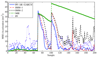
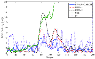
The performance of the IMM algorithms, MIE scheme, PF approach and the PF-AR-GARCH method are shown in Fig. 2 for this simulation. It can be seen that the PF-AR-GARCH method outperforms the IMM schemes when the target is in the transition period. In the steady state of the accelerating interval, some advantages can also be obtained through the proposed PF-AR-GARCH model but the improvement is generally not so significant as that in the transition case. In addition, the effect of transition probability matrix is obvious, especially in the constant acceleration period for the acceleration estimation and in the transition interval for the velocity estimation. Although the performance of the IMM methods is better than the proposed method in the CV interval, the proposed PF-AR-GARCH method outperforms in the other time intervals, i.e. the transition periods and CA intervals, which are more important in the maneuver target tracking applications.

In comparison with MIE model, the PF-AR-GARCH algorithm has a better performance in transition and constant acceleration periods. In Fig. 2(a), the performance of MIE is eliminated after 100 samples due to an unacceptable performance and make the figure more clear. The PF algorithm shows weak performance in the CV interval compared with the other approaches. Although the performance of the PF is better than IMMs and MIE algorithms in the transition period especially for velocity estimation, the performance of PF-AR-GARCH approach is superior than PF for acceleration and velocity estimation in this period. The estimation delay for the PF is illustrated in the transition period. However, the PF performance is degraded in the CA interval in comparison with the proposed PF-AR-GARCH method.

TABLE II: The RMSE Result of Different Methods by 1000 Monte Carlo Simulations for Test Trajectory 1 (High Maneuver)

RMSE	Position [$m$]	Velocity [$m/s$]	Acceleration [$m/s^{2}$]
PF-AR-GARCH	2.0566	1.2849	2.4288
IMM-1	2.0732	1.5256	2.5194
IMM-2	2.2313	1.8617	3.4251
MIE	5.4701	5.9399	5.0973
PF	4.6599	1.9908	3.3066

Figure 3: The Number of Particles versus the MSE of PF-AR-GARCH method for Test Trajectory 1 (High Maneuver)

The root mean square error (RMSE) of the proposed method in comparison with the IMM-1, IMM-2, MIE and PF algorithms, is shown in Table II. Some Monte Carlo simulations with $1000$ runs in each simulation are performed. It is seen that the improvement, due to the proposed PF-AR-GARCH, is rather significant, especially in the velocity and acceleration estimations. As we mentioned in the introduction, more accurate estimations in the velocity and acceleration are particularly useful in some applications such as threat evaluation, etc. According to the PF results in Fig. 2 and Table II, we can conclude that the PF algorithms without considering the proper model does not have good performance. This test illustrates the significant effect of the proposed GARCH model for the maneuvering target tracking applications.

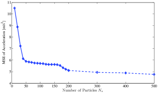
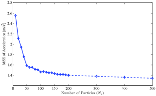
Fig. 3 illustrates the effect of number of particles for the bootstrapped PF-AR-GARCH tracking in the test trajectory $1$ when the other parameters are fixed. The more $N_{s}$ provide the less RMSE for the proposed method while the IMM and MIE are not dependent on this degree of freedom, but, this higher accuracy provided by bootstrapping comes at an extra computational cost as denoted in Table I. According to the Fig. 3, $N_{s}=50$ is selected to reduce the computational complexity in this simulation.

VI-A2 Example B

In this example, we consider the sampling time is $T=0.05s$, the initial position of target is $\boldmath{X}(t)=[2000m,\,10000m,\,0m/s,\,-15m/s],$ the variances of the measurement noises are $\sigma_{Position}^{2}=10^{4}m,$ and $\sigma_{Velocity}^{2}=25m/s$, and the process noise is zero for the trajectory simulation. The target is assumed to move with a constant velocity until time $t=5s$ in $X$ direction, and the $Y$ direction of the velocity is constant until time $t=3.5s$. The target begins to maneuver at an acceleration of $U_{y}=1m/s^{2}$ for the sample interval $[70,200]$. In the sample interval $[100,200]$, a constant acceleration $U_{x}=0.8m/s^{2}$ is applied in $X$ direction. In this simulation, $N_{s}=50$ is selected based on Fig. 4. The standard deviation parameters of IMM are selected to be $\sigma_{CA}=1U_{y}=1$ and $\sigma_{CV}=0.1\sigma_{CA}=0.1,$ for the CA and CV models, respectively. The transition probability matrix between the two models is given by $p_{ij}=[0.99\quad 0.01;\quad 0.01\quad 0.99].$ According to the best scenario, the variance parameters of the PF and MIE methods are selected to be $\sigma_{PF}^{2}=5$ and $\sigma_{MIE}^{2}=5$, respectively. The number of particles in PF algorithms is selected to be $N_{s}=200$.

This example describes a low maneuver behavior to demonstrate the performance of PF-AR-GARCH approach compared with the other methods. Table III shows the RMSE of proposed method in comparison with the IMM, MIE and PF algorithms. Some Monte Carlo simulations with $1000$ runs in each simulation are performed. It is seen that the proposed PF-AR-GARCH scheme has a better performance for an approximately non-jumpy situation. Therefore, we conclude that PF-AR-GARCH is appropriate equivalently for low and high maneuver behaviors.

TABLE III: The RMSE Result of Different Methods by 1000 Monte Carlo Simulations for Test Trajectory 1 (Low Maneuver)

RMSE	Position [$m$]	Velocity [$m/s$]	Acceleration [$m/s^{2}$]
PF-AR-GARCH	2.0462	1.1631	0.7735
IMM	2.1622	1.2897	1.0211
MIE	9.0189	3.7593	1.6243
PF	4.6938	1.7110	1.4165

Figure 4: The Number of Particles versus the MSE of PF-AR-GARCH method for Test Trajectory 1 (Low Maneuver)

VI-B Test trajectory 2

In this test, the trajectory is simulated by heavy-tailed property assumption of the state equation noise. As we noted in the introduction, there are some rich literatures on modeling heavy-tailed system noise [30, 53]. Our main purpose is to develop a model where a maneuver can be considered as independent heavy-tailed noise to one or more of the state variables. The reason for this assumption is that the unimodal heavy-tail distribution represents usually small fluctuations and abrupt changes of acceleration in a simultaneous manner.

For this test problem, the target’s motion equation is expressed in terms of the non-Gaussian noise as follows:

$$\mbox{\boldmath$\dot{X}$}(t)=\mbox{\boldmath$F$}\mbox{\boldmath$X$}(t)+\mbox{\boldmath$G$}\mbox{\boldmath$\vartheta$}(t)$$

where $\mbox{\boldmath$X$}(t)=\left[\mbox{\boldmath$x$}(t)^{T}\>\mbox{\boldmath$v$}(t)^{T}\>\mbox{\boldmath$a$}(t)\right]^{T}$ denotes a six-dimensional position-velocity-acceleration parameter vector and $\mbox{\boldmath$\vartheta$}(t)=[\vartheta_{x}(t)\>\vartheta_{y}(t)]^{T}$ is the non-Gaussian system noise vector. In this simulation trial, the true target trajectory is simulated with independent random initial position, velocity, and acceleration. The true process noise is set to be student-$t$ with one degree of freedom. The position and velocity of the target are measured every $T=1s$. We have set the parameters value of IMM as $\sigma_{CV}^{2}=0.1,$ $\sigma_{CA}^{2}=10$, and $p_{ij}=[0.8\quad 0.2;\quad 0.2\quad 0.8]$. On the other hand, the parameters of the EKF-IMM and UKF-IMM approaches are selected to be $\sigma_{CV}^{2}=1$, $\sigma_{CA}^{2}=5$ and $\sigma_{CT}^{2}=10$. In addition, the transition probability matrix between the three models in the EKF-IMM and UKF-IMM methods is given by $p_{ij}=[0.99\quad 0.01\quad 0.00;0.33\quad 0.34\quad 0.33;0.00\quad 0.01\quad 0.99]$. In this simulation, the selection of IMM parameters is based on a trade off between the performance of steady state and transition estimations as well as the previous test. The MIE parameters are selected according to the best performance as $\sigma^{2}=100$.

TABLE IV: The RMSE Result of Different Methods by 1000 Monte Carlo Simulations for Test Trajectory 2 (Student-$t$ Distribution)

RMSE	Position [$m$]	Velocity [$m/s$]	Acceleration [$m/s^{2}$]
PF-AR-GARCH	6.0612	2.0857	1.5900
IMM	6.4961	2.5270	2.4861
EKF-IMM	6.4458	2.5204	2.3709
UKF-IMM	6.2996	2.5052	2.1559
MIE	41.7349	9.2089	3.0882
PF	30.8065	7.5206	2.7412

Figure 5: The Number of Particles versus the MSE of PF-AR-GARCH method for Test Trajectory 2

For the quantitative comparison, the RMSE of tracking results are calculated. To achieve more precise results, some Monte Carlo simulations with 1000 runs is obtained in each algorithm and the RMSE values of the estimation are computed by averaging. The results are illustrated in Table IV. We can draw two important conclusions from Table IV. First, the proposed GARCH approach can handle non-Gaussianity more properly. Second, the effect of estimation delay in the MIE for high maneuvering trajectories causes large RMSE.

Fig. 5 illustrates the effect of particles number for the bootstrapped PF-AR-GARCH tracking in test trajectory $2$ when the other parameters are fixed. According to the Fig. 5, the number of particles, $N_{s}$ is selected $50$ in order to reduce the computational complexity in this test trajectory.

VI-C Test trajectory 3

The main goal of this study is (a) to show that the proposed model is so general that can describe several different motion models, and (b) to illustrate the sensitivity of IMM method to the priori parameters, i.e. variance of the state models and the model transition probability matrix. Moreover, this simulation shows that the dynamics are difficult to break up into several different motion models in IMM methods. When the parameters are changed to get better performance in one situation, the other interval of the tracking have a bad performance and vice versa. In order to provide better understanding of the IMM influence design variables, three IMMs are simulated. We considered the noise standard deviation of the state models of IMM-1, IMM-2 and IMM-3 as $\sigma_{CV}=0.1\sigma_{CA}^{2}=1.5$, $\sigma_{CV}=0.1\sigma_{CA}=0.8$, and $\sigma_{CV}=0.1\sigma_{CA}=0.5$, respectively. The model transition probability matrix $p_{ij}=[0.85\quad 0.15;\quad 0.15\quad 0.85]$ is considered for three IMMs. The noise variance of the MIE method is considered as $\sigma_{X}^{2}=1000$. The sampling time is $T=1s$ and the number of the samples are 200. Initial position is assumed to be $\mbox{\boldmath$X$}(0)=[10m,-10m,10m/s,15m/s]^{T}$. $N_{s}=400$ shows the best performance in the PF method for this scenario.

TABLE V: The RMSE Result of Different Methods by 1000 Monte Carlo simulations for Test Trajectory 3

RMSE	Position [$m$]	Velocity [$m/s$]	Acceleration [$m/s^{2}$]
PF-AR-GARCH	2.3029	1.6263	1.9365
IMM-1	3.7540	3.1086	2.1046
IMM-2	2.6401	2.4952	2.1206
IMM-3	3.2011	2.9341	2.2144
MIE	20.7740	3.9147	3.3100
PF	8.3287	3.7210	2.9695

Figure 6: The Number of Particles versus the MSE of PF-AR-GARCH method for Test Trajectory 3

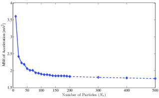
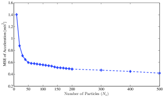
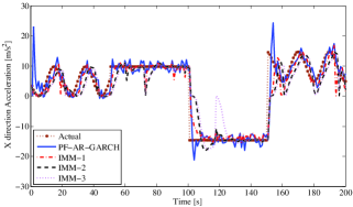
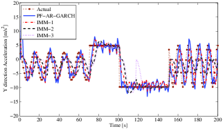
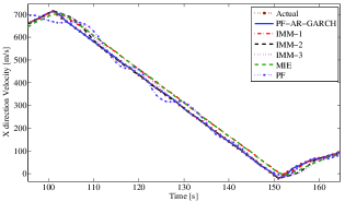
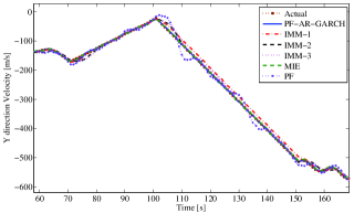
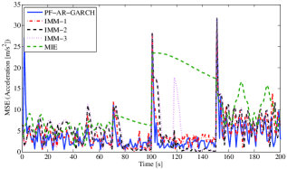
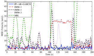
Fig. 6 illustrates the effect of number of particles for the bootstrapped PF-AR-GARCH tracking in test trajectory $3$ when the other parameters are fixed. According to the Fig. 6, $N_{s}=100$ is selected in order to reduce the computational complexity in this test trajectory. Fig. 7 and Fig. 8 show the estimated and actual values for acceleration and velocity of the target, respectively, which are achieved by the PF-AR-GARCH, IMM, MIE and PF approaches. Moreover, each algorithm is simulated 1000 times and the final RMSE is illustrated in Table V. Since the performances of the MIE and PF algorithms are not acceptable, their results are eliminated from Fig. 7 to improve the quality of this figure. The simulation results show that the proposed algorithm outperforms IMM methods, especially in sinusoidal case. According to the Fig. 7, at the time $t=100s$, the target acceleration changes drastically. The GARCH model follows this sinusoidal trajectory quite well, whereas IMM does not. In the time interval $100s<t<150s$ after the abrupt changes in time instant $t=100s$, the value of conditioned likelihood function in the CV model is extremely larger than the CA model for IMM-1. Then, the IMM method allocates higher weights to the CV model in this time interval, near one. Therefore, the difference of velocity is used as the estimation of acceleration on this time slot. This approach provides a better performance to acceleration estimation of IMM-1. Table V demonstrates that the IMM-1 has a good performance in the acceleration estimation compared with the other IMMs, however, its performance to the position and velocity estimations is lower than IMM-2 and IMM-3. Fig. 8 shows this unacceptable performance of IMM-1 to estimate the position and velocity. According to Fig. 8, the velocity estimation of IMM-1 is weak. These differences among three IMMs tracking accuracies provide a conclusion that IMM algorithm is sensitive to the priori information. The variance of process noise of the IMM-1 results in a weak performance to velocity estimation in the interval $100s<t<150s$, whereas, an acceptable accuracy to acceleration estimation is resulted in the sinusoidal intervals. Moreover, the performance of the IMM-2 is increased in the constant acceleration with decrease in the variance of the process noise. However, its performance is degraded in the sinusoidal interval. The decrease of the noise variance in the IMM-3 shows an inappropriate effect in the $100s<t<150s$ interval.

For better comparison, we also evaluate MSE of estimated acceleration by running a simulation for the above methods. The results are depicted in Fig. 9. However, the results of the PF approach and some time intervals of MIE algorithm are excluded from Fig. 9 because they do not perform well in this scenario.

(a)

(b)

Figure 7: The actual and the estimated acceleration in (a) x direction and (b) y direction

(a)

(b)

Figure 8: The actual and the estimated velocity in (a) x direction and (b) y direction

(a)

(b)

Figure 9: The MSE of different methods in 200 sec for (a) acceleration and (b) velocity

VII Conclusion

In this paper, we introduced a semi-parametric category of the target tracking. The parameters are embedded in AR-GARCH modeling of volatility process. The stochastic volatility and target’s state are estimated by a bootstrap PF, simultaneously. We proposed maneuvering motion model of a target using an SDE whose volatility is subsequently modeled by a GARCH process. This approach allowed us to evaluate the performance of SDE model based on GARCH process for tracking a maneuvering target with abrupt changes in its acceleration. It is shown that the GARCH model provides finer tracking accuracy for high maneuvering target by using heavy tailed distribution modeling, i.e. GARCH, instead of Gaussian distribution adopted by IMM, MIE, and etc., for system noise of state space model. The simulation results determine that the proposed PF-AR-GARCH approach, models and tracks abrupt changes in acceleration more accurately. Consequently, the proposed stochastic volatility modeling enhances maneuvering target tracking performance.

Appendix A Conditional Heteroscedasticity of Acceleration

In this appendix, we show that the stochastic property of autoregression coefficient of acceleration, $\zeta(k)$, in (5) results conditional heteroscedasticity. If we suppose that the immediate past information for acceleration is $\Psi_{k-1}=\{a(0),a(1),\cdots,{a(k-1)},w(0),w(1),\cdots,w(k-1)\}$, the conditional mean of $a(k)$ will be obtained be conditional expectation of (5):

$$E\left.\left\{a(k)\right|\Psi_{k-1}\right\}=E\left.\left\{\zeta(k)\right|\Psi_{k-1}\right\}a(k-1)$$ (40)

Using (40), the conditional variance of $a(k)$ is written as:

$$\mbox{Var}\left.\left\{a(k)\right|\Psi_{k-1}\right\}$$

$$=E\left.\left\{\left(a(k)-E\left.\left\{\zeta(k)\right|\Psi_{k-1}\right\}a(k-1)\right)^{2}\right|\Psi_{k-1}\right\}$$

$$=E\left.\left\{\left(\zeta(k)a(k-1)-E\left.\left\{\zeta(k)\right|\Psi_{k-1}\right\}a(k-1)+w(k)\right)^{2}\right|\Psi_{k-1}\right\}$$

$$=\sigma_{\zeta}^{2}a^{2}(k-1)+\sigma^{2}_{m}.$$ (41)

According to (A), it is clear that conditional variance of $a(k)$ is not constant in time, then, $a(k)$ is conditional heteroscedastic.

Appendix B Covariance Matrix Calculation

In this appendix, we solve the stochastic It$\bar{\mbox{o}}$ integral to obtain the suggested time-varying covariance matrix for maneuvering target tracking application proposed in this paper which is applied in bootstrap PF procedure. To achieve this, we begin with equation (22). We suppose that the SV, $\mbox{\boldmath$H$}(s)$, is constant and set to $\mbox{\boldmath$H$}(kT)$ in the integration interval $[kT,kT+T)$, which is estimated based on GARCH process in the filtering procedure. Thus,

$$\mbox{\boldmath$U$}(k) = \int_{kT}^{kT+T}\exp(\mbox{\boldmath$F$}(kT+T-s))\mbox{\boldmath$G$}\mbox{\boldmath$H$}^{\frac{1}{2}}(kT)d\mbox{\boldmath$W$}(s)$$ (50)

$$= \int_{kT}^{kT+T}\mbox{\boldmath$\Phi$}(kT+T-s,\mu)\mbox{\boldmath$G$}\mbox{\boldmath$H$}^{\frac{1}{2}}(kT)d\mbox{\boldmath$W$}(s)$$

$$= \int_{kT}^{kT+T}\left[{\begin{array}[]{*{20}{c}}{\mbox{\boldmath$\varphi$}_{1}(s)}\\ {\mbox{\boldmath$\varphi$}_{2}(s)}\\ {\exp(-\mu(kT+T-s))\mbox{\boldmath$I$}_{2\times 2}}\end{array}}\right]$$

$$\left[{\begin{array}[]{*{20}{c}}{\sqrt{h_{x}(kT)}}&{0}\\ {0}&{\sqrt{h_{y}(kT)}}\end{array}}\right]\left[{\begin{array}[]{*{20}{c}}{dW_{x}(s)}\\ {dW_{y}(s)}\end{array}}\right],$$

where $\mbox{\boldmath$\varphi_{1}$}(s)=\varphi_{1}(kT+T-s,\mu)\mbox{\boldmath$I$}_{2\times 2}$ and $\mbox{\boldmath$\varphi_{2}$}(s)=\varphi_{2}(kT+T-s,\mu)\mbox{\boldmath$I$}_{2\times 2}$. Then, we easily have:

$$\mbox{\boldmath$U$}(k)=\int_{kT}^{kT+T}\left[{\begin{array}[]{*{20}{c}}{{\gamma_{1x}(s)}}&0\\ 0&{{\gamma_{1y}(s)}}\\ {{\gamma_{2x}(s)}}&0\\ 0&{{\gamma_{2y}(s)}}\\ {\gamma_{3x}(s)}&0\\ 0&{\gamma_{3y}(s)}\end{array}}\right]\left[{\begin{array}[]{*{20}{c}}{dW_{x}(s)}\\ {dW_{y}(s)}\end{array}}\right],$$ (51)

where

$$\gamma_{1x}(s) = \varphi_{1}(kT+T-s,\mu)\sqrt{h_{x}(kT)},$$

$$\gamma_{1y}(s) = \varphi_{1}(kT+T-s,\mu)\sqrt{h_{y}(kT)},$$

$$\gamma_{2x}(s) = \varphi_{2}(kT+T-s,\mu)\sqrt{h_{x}(kT)},$$

$$\gamma_{2y}(s) = \varphi_{2}(kT+T-s,\mu)\sqrt{h_{y}(kT)},$$

$$\gamma_{3x}(s) = \exp(-\mu(kT+T-s))\sqrt{h_{x}(kT)},$$

$$\gamma_{3y}(s) = \exp(-\mu(kT+T-s))\sqrt{h_{y}(kT)},$$

and we define matrix $\mbox{\boldmath$\Gamma$}(s)$ as follow:

$$\mbox{\boldmath$\Gamma$}(s)=\left[{\begin{array}[]{*{20}{c}}{{\gamma_{1x}(s)}}&0\\ 0&{{\gamma_{1y}(s)}}\\ {{\gamma_{2x}(s)}}&0\\ 0&{{\gamma_{2y}(s)}}\\ {\gamma_{3x}(s)}&0\\ 0&{\gamma_{3y}(s)}\end{array}}\right].$$ (52)

Thus

$$\mbox{\boldmath$U$}(k)=\int_{kT}^{kT+T}\mbox{\boldmath$\Gamma$}(s)\left[{\begin{array}[]{*{20}{c}}{dW_{x}(s)}\\ {dW_{y}(s)}\end{array}}\right].$$ (53)

According to the input vector $\mbox{\boldmath$U$}(k)$ in equation (53), $E\left\{{\mbox{\boldmath$U$}(k)\mbox{\boldmath$U$}^{T}(i)}\right\}$ can be calculated as follow:

$$E\left\{{\mbox{\boldmath$U$}(k)\mbox{\boldmath$U$}^{T}(i)}\right\}=$$ (58)

$$E\biggr{\{}\int_{kT}^{kT+T}\mbox{\boldmath$\Gamma$}(s)\left[{\begin{array}[]{*{20}{c}}{dW_{x}(s)}\\ {dW_{y}(s)}\end{array}}\right]\int_{iT}^{iT+T}\left[{\begin{array}[]{*{20}{c}}{dW_{x}(\tau)}\\ {dW_{y}(\tau)}\end{array}}\right]^{T}\mbox{\boldmath$\Gamma$}^{T}(\tau)\biggr{\}}$$

$$= \int_{kT}^{kT+T}\!\!\!\!\int_{iT}^{iT+T}\!\!\!\!\mbox{\boldmath$\Gamma$(s)}E\biggr{\{}\!\!\left[{\begin{array}[]{*{20}{c}}{dW_{x}(s)}\\ {dW_{y}(s)}\end{array}}\right]\!\!\left[{\begin{array}[]{*{20}{c}}{dW_{x}(\tau)}\\ {dW_{y}(\tau)}\end{array}}\right]^{T}\biggr{\}}\mbox{\boldmath$\Gamma$}^{T}(\tau).$$ (63)

According to Brownian motion properties [45], independent increments and zero-mean Gaussian distribution in an increment, when $k\neq i$,

$$E\biggr{\{}\!\!\left[{\begin{array}[]{*{20}{c}}{dW_{x}(s)}\\ {dW_{y}(s)}\end{array}}\right]\!\!\left[{\begin{array}[]{*{20}{c}}{dW_{x}(\tau)}\\ {dW_{y}(\tau)}\end{array}}\right]^{T}\biggr{\}}=\mbox{\boldmath$0$}_{2\times 2}$$

then, $E\left\{{\mbox{\boldmath$U$}(k)\mbox{\boldmath$U$}^{T}(i)}\right\}=\mbox{\boldmath$0$}_{2\times 2}$. The covariance matrix $\mbox{\boldmath$Q$}(k)$ satisfies, using (58),

$$\mbox{\boldmath$Q$}(k) = E\left\{{\mbox{\boldmath$U$}(k)\mbox{\boldmath$U$}^{T}(k)}\right\}$$ (64)

$$= \mathop{\int\int}_{\!\!\!kT}^{KT+T}\!\mbox{\boldmath$\Gamma$(s)}d\mbox{\boldmath$B$}(s,\tau)\mbox{\boldmath$\Gamma$}^{T}(\tau)$$

where

$$d\mbox{\boldmath$B$}(s,\tau)=E\biggr{\{}\!\!\left[{\begin{array}[]{*{20}{c}}{dW_{x}(s)dW_{x}(\tau)}&\quad{dW_{x}(s)dW_{y}(\tau)}\\ {dW_{y}(s)dW_{x}(\tau)}&\quad{dW_{y}(s)dW_{y}(\tau)}\end{array}}\right]\biggr{\}}.$$ (65)

The Brownian motions in directions $x$ and $y$ are independent processes from each other, so that $E\{dW_{x}dW_{y}\}=0$. Accordingly, $d\mbox{\boldmath$B$}(s,\tau)$ is a diagonalized matrix and (65) is verified by It$\bar{\mbox{o}}$ calculation, $E\{dW_{x}(s)dW_{x}(\tau)\}=\delta(s-\tau)dsd\tau$, and can be written as

$$d\mbox{\boldmath$B$}(s,\tau)=[\delta(s-\tau)dsd\tau]\mbox{\boldmath$I$}_{2\times 2}.$$ (66)

By inserting (66) in (64) the covariance matrix $\mbox{\boldmath$Q$}(k)$ required for bootstrapping of PF is expressed as

$$\mbox{\boldmath$Q$}(k)=\int_{kT}^{kT+T}\mbox{\boldmath$\Gamma$}(s)\mbox{\boldmath$\Gamma$}^{T}(s)ds.$$ (67)

By substituting (52) in (67) and computing the Riemann integral, the matrix $\mbox{\boldmath$Q$}(k)$ will be obtained.

References

- [1] Yihua Yu and Qiansheng Cheng, “Particle filters for maneuvering target tracking problem,” Signal Processing, vol. 86, no. 1, pp. 195–203, 2006.
- [2] Katrin Achutegui, Joaquin Miguez, Javier Rodas, and Carlos J Escudero, “A multi-model sequential monte carlo methodology for indoor tracking: Algorithms and experimental results,” Signal Processing, vol. 92, no. 11, pp. 2594–2613, 2012.
- [3] Taek Lyul Song, Darko Musicki, and Kim Da Sol, “Target tracking with target state dependent detection,” IEEE Transactions on Signal Processing, vol. 59, no. 3, pp. 1063–1074, 2011.
- [4] Ehsan Hajiramezanali, Mahdi Imani, Ulisses Braga-Neto, Xiaoning Qian, and Edward R Dougherty, “Scalable optimal bayesian classification of single-cell trajectories under regulatory model uncertainty,” in Proceedings of the 2018 ACM International Conference on Bioinformatics, Computational Biology, and Health Informatics. ACM, 2018, pp. 596–597.
- [5] Andrew Logothetis, Vikram Krishnamurthy, and Jan Holst, “A bayesian em algorithm for optimal tracking of a maneuvering target in clutter,” Signal processing, vol. 82, no. 3, pp. 473–490, 2002.
- [6] Robert A Singer, “Estimating optimal tracking filter performance for manned maneuvering targets,” IEEE Transactions on Aerospace and Electronic Systems, , no. 4, pp. 473–483, 1970.
- [7] Yaakov Bar-Shalom and Kailash Birmiwal, “Variable dimension filter for maneuvering target tracking,” IEEE transactions on Aerospace and Electronic Systems, , no. 5, pp. 621–629, 1982.
- [8] PL Bogler, “Tracking a maneuvering target using input estimation,” IEEE transactions on Aerospace and Electronic Systems, , no. 3, pp. 298–310, 1987.
- [9] Ick Ho Whang, Jang Gyu Lee, and Tae Kyung Sung, “Modified input estimation technique using pseudoresiduals,” IEEE transactions on aerospace and electronic systems, vol. 30, no. 1, pp. 220–228, 1994.
- [10] X Rong Li and Vesselin P Jilkov, “Survey of maneuvering target tracking. Part I. Dynamic models,” IEEE Transactions on aerospace and electronic systems, vol. 39, no. 4, pp. 1333–1364, 2003.
- [11] Hongda Chen and KC Chang, “Novel nonlinear filtering & prediction method for maneuvering target tracking,” IEEE Transactions on Aerospace and Electronic Systems, vol. 45, no. 1, pp. 237–249, 2009.
- [12] Nassib Nabaa and Robert H Bishop, “Validation and comparison of coordinated turn aircraft maneuver models,” IEEE Transactions on aerospace and electronic systems, vol. 36, no. 1, pp. 250–259, 2000.
- [13] James P Helferty, “Improved tracking of maneuvering targets: The use of turn-rate distributions for acceleration modeling,” IEEE Transactions on Aerospace and Electronic Systems, vol. 32, no. 4, pp. 1355–1361, 1996.
- [14] Hungu Lee and Min-Jea Tahk, “Generalized input-estimation technique for tracking maneuvering targets,” IEEE transactions on Aerospace and Electronic Systems, vol. 35, no. 4, pp. 1388–1402, 1999.
- [15] YT Chan, AGC Hu, and JB Plant, “A kalman filter based tracking scheme with input estimation,” IEEE transactions on Aerospace and Electronic Systems, , no. 2, pp. 237–244, 1979.
- [16] Liu Jing and Prahlad Vadakkepat, “Interacting mcmc particle filter for tracking maneuvering target,” Digital Signal Processing, vol. 20, no. 2, pp. 561–574, 2010.
- [17] Fun-Bin Duh and Chin-Teng Lin, “Tracking a maneuvering target using neural fuzzy network,” IEEE Transactions on Systems, Man, and Cybernetics, Part B (Cybernetics), vol. 34, no. 1, pp. 16–33, 2004.
- [18] Tae K Sung and Jang Gyu Lee, “A decoupled adaptive tracking filter for real applications,” IEEE transactions on aerospace and electronic systems, vol. 33, no. 3, pp. 1025–1030, 1997.
- [19] Ali Karsaz and Hamid Khaloozadeh, “An optimal two-stage algorithm for highly maneuvering targets tracking,” Signal processing, vol. 89, no. 4, pp. 532–547, 2009.
- [20] Jitendra K Tugnait, “Detection and estimation for abruptly changing systems,” Automatica, vol. 18, no. 5, pp. 607–615, 1982.
- [21] Yaakov Bar-Shalom, X Rong Li, and Thiagalingam Kirubarajan, Estimation with applications to tracking and navigation: theory algorithms and software, John Wiley & Sons, 2004.
- [22] Henk AP Blom and Yaakov Bar-Shalom, “The interacting multiple model algorithm for systems with markovian switching coefficients,” IEEE transactions on Automatic Control, vol. 33, no. 8, pp. 780–783, 1988.
- [23] Leigh A Johnston and Vikram Krishnamurthy, “An improvement to the interacting multiple model (imm) algorithm,” IEEE transactions on signal processing, vol. 49, no. 12, pp. 2909–2923, 2001.
- [24] X Rong Li and Yaakov Bar-Shalom, “Performance prediction of the interacting multiple model algorithm,” IEEE Transactions on Aerospace and Electronic Systems, vol. 29, no. 3, pp. 755–771, 1993.
- [25] Thia Kirubarajan, Yaakov Bar-Shalom, Krishna R Pattipati, and Ivan Kadar, “Ground target tracking with variable structure imm estimator,” IEEE Transactions on Aerospace and Electronic Systems, vol. 36, no. 1, pp. 26–46, 2000.
- [26] I Bilik and J Tabrikian, “Maneuvering target tracking in the presence of glint using the nonlinear gaussian mixture kalman filter,” IEEE Transactions on Aerospace and Electronic Systems, vol. 46, no. 1, 2010.
- [27] K Punithakumar, T Kirubarajan, and A Sinha, “Multiple-model probability hypothesis density filter for tracking maneuvering targets,” IEEE Transactions on Aerospace and Electronic Systems, vol. 44, no. 1, pp. 87–98, 2008.
- [28] Xuezhi Wang, Subhash Challa, Rob Evans, and X Rong Li, “Minimal submodel-set algorithm for maneuvering target tracking,” IEEE Transactions on Aerospace and Electronic Systems, vol. 39, no. 4, pp. 1218–1231, 2003.
- [29] Tan-Jan Ho and Bor-Sen Chen, “Novel extended viterbi-based multiple-model algorithms for state estimation of discrete-time systems with markov jump parameters,” IEEE Transactions on Signal Processing, vol. 54, no. 2, pp. 393–404, 2006.
- [30] A Sinha, T Kirubarajan, and Y Bar-Shalom, “Application of the kalman-levy filter for tracking maneuvering targets,” IEEE Transactions on Aerospace and Electronic Systems, vol. 43, no. 3, 2007.
- [31] Mohammadehsan Hajiramezanali and Hamidreza Amindavar, “Maneuvering target tracking based on combined stochastic differential equations and garch process,” in Information Science, Signal Processing and their Applications (ISSPA), 2012 11th International Conference on. IEEE, 2012, pp. 1293–1297.
- [32] Mohammadehsan Hajiramezanali and Hamidreza Amindavar, “Maneuvering target tracking based on sde driven by garch volatility,” in Statistical Signal Processing Workshop (SSP), 2012 IEEE. IEEE, 2012, pp. 764–767.
- [33] Mohammadehsan Hajiramezanali, Seyyed Hamed Fouladi, James A Ritcey, and Hamidreza Amindavar, “Stochastic differential equations for modeling of high maneuvering target tracking,” ETRI Journal, vol. 35, no. 5, pp. 849–858, 2013.
- [34] Jiin-An Guu and Che-Ho Wei, “Maneuvering target tracking using imm method at high measurement frequency,” IEEE Transactions on Aerospace and Electronic Systems, vol. 27, no. 3, pp. 514–519, 1991.
- [35] Robert F Engle, “Autoregressive conditional heteroscedasticity with estimates of the variance of united kingdom inflation,” Econometrica: Journal of the Econometric Society, pp. 987–1007, 1982.
- [36] Tim Bollerslev, “Generalized autoregressive conditional heteroskedasticity,” Journal of econometrics, vol. 31, no. 3, pp. 307–327, 1986.
- [37] Saman Mousazadeh and Israel Cohen, “Ar-garch in presence of noise: Parameter estimation and its application to voice activity detection,” IEEE Transactions on Audio, Speech, and Language Processing, vol. 19, no. 4, pp. 916–926, 2011.
- [38] Ehsan Hajiramezanali, Siamak Zamani Dadaneh, Paul de Figueiredo, Sing-Hoi Sze, Mingyuan Zhou, and Xiaoning Qian, “Differential expression analysis of dynamical sequencing count data with a gamma markov chain,” arXiv preprint arXiv:1803.02527, 2018.
- [39] David S Matteson and David Ruppert, “Time-series models of dynamic volatility and correlation,” IEEE Signal Processing Magazine, vol. 28, no. 5, pp. 72–82, 2011.
- [40] Tim Bollerslev, Ray Y Chou, and Kenneth F Kroner, “Arch modeling in finance: A review of the theory and empirical evidence,” Journal of econometrics, vol. 52, no. 1-2, pp. 5–59, 1992.
- [41] P Reinhard Hansen and Asger Lunde, “Does anything beat a garch (1, 1)? a comparison based on test for superior predictive ability,” in Computational Intelligence for Financial Engineering, 2003. Proceedings. 2003 IEEE International Conference on. IEEE, 2003, pp. 301–307.
- [42] Seyyed Hamed Fouladi, Mohammadehsan Hajiramezanali, Hamidreza Amindavar, James A Ritcey, and Payman Arabshahi, “Denoising based on multivariate stochastic volatility modeling of multiwavelet coefficients.,” IEEE Trans. Signal Processing, vol. 61, no. 22, pp. 5578–5589, 2013.
- [43] John C Cox, Jonathan E Ingersoll Jr, and Stephen A Ross, “A theory of the term structure of interest rates,” in Theory of Valuation, pp. 129–164. World Scientific, 2005.
- [44] Ole E Barndorff-Nielsen and Neil Shephard, “Non-gaussian ornstein–uhlenbeck-based models and some of their uses in financial economics,” Journal of the Royal Statistical Society: Series B (Statistical Methodology), vol. 63, no. 2, pp. 167–241, 2001.
- [45] Bernt Øksendal, “Stochastic differential equations,” in Stochastic differential equations, pp. 65–84. Springer, 2003.
- [46] Arthur Gelb, Applied optimal estimation, MIT press, 1974.
- [47] Ehsan Hajiramezanali, Siamak Zamani Dadaneh, Alireza Karbalayghareh, Mingyuan Zhou, and Xiaoning Qian, “Bayesian multi-domain learning for cancer subtype discovery from next-generation sequencing count data,” in Advances in Neural Information Processing Systems, 2018, pp. 9133–9142.
- [48] Arnaud Doucet and Adam M Johansen, “A tutorial on particle filtering and smoothing: Fifteen years later,” Handbook of nonlinear filtering, vol. 12, no. 656-704, pp. 3, 2009.
- [49] Shaun McGinnity and George W Irwin, “Multiple model bootstrap filter for maneuvering target tracking,” IEEE Transactions on Aerospace and Electronic systems, vol. 36, no. 3, pp. 1006–1012, 2000.
- [50] Shaun McGinnity and George W Irwin, “Manoeuvring target tracking using a multiple-model bootstrap filter,” in Sequential Monte Carlo Methods in Practice, pp. 479–497. Springer, 2001.
- [51] Ben North, Andrew Blake, Michael Isard, and Jens Rittscher, “Learning and classification of complex dynamics,” IEEE Transactions on Pattern Analysis & Machine Intelligence, , no. 9, pp. 1016–1034, 2000.
- [52] YT Chan, AGC Hu, and JB Plant, “A kalman filter based tracking scheme with input estimation,” IEEE transactions on Aerospace and Electronic Systems, , no. 2, pp. 237–244, 1979.
- [53] N Ikoma, T Higuchi, and H Maeda, “Tracking of maneuvering target by using switching structure and heavy-tailed distribution with particle filter method,” in Control Applications, 2002. Proceedings of the 2002 International Conference on. IEEE, 2002, vol. 2, pp. 1282–1287.