Nonsteady-state diffusion in two-dimensional periodic channels

Abstract

The dynamics of a freely diffusing particle in a two-dimensional channel with cross sectional area $A(x)$, can be effectively described by a one-dimensional diffusion equation under the action of a potential of mean force $U(x)=-k_{B}T\ln[A(x)]$ (where $k_{B}T$ is the thermal energy) in a system with a spatially-dependent diffusion coefficient $D(x)$. Several attempts to derive expressions relating $D(x)$ to $A(x)$ and its derivatives have been made, which were based on considering stationary flows in periodic channels. Here, we take an alternative approach and consider non-steady state single particle diffusion in an open periodic channel. The approach allows us to express $D(x)$ as a series of terms of increasing powers of $\epsilon$ - a parameter associated with the aspect ratio of the channel. When the expansion is truncated at the leading term, we recover the expression suggested by Zwanzig [J. Phys. Chem. 96, 3926 (1992)] for $D(x)$. Furthermore, comparison of the first few terms in our expansion for $D(x)$ with the one proposed by Kalinay and Percus [Phys. Rev. E 74, 041203 (2006)] shows that they are consistent with each other. In the limit of long wavelength channels ($\epsilon\ll 1$), the expansion converges rapidly and the leading approximation provides a very accurate description of the two-dimensional dynamics. For short wavelength channels, the expansion does not converge and the validity of the effective one-dimensional description is questionable.

I Introduction

Transport of particles in narrow corrugated channels has received a considerable attention in the past fifteen years. The reason for the growing interest in problems of this type is their relevance to numerous naturally occurring systems such as membrane ion channel [1], carbon nanotubes [2], zeolites [3], etc. Understanding molecular dynamics in narrow channels is also important for many technological applications, e.g., microfluidic devices [4] and solid state nanopores [5].

In this context, there have been numerous theoretical studies of the following problem: Consider a particle moving in an open two-dimensional channel whose long axis lies along the $x$-direction ($-\infty<x<\infty$). In the perpendicular $y$ direction, the channel is bounded between $0\leq y\leq A(x)$, where $A(x)$ is a periodic function with wavelength $\lambda$. The two-dimensional (2D) probability density, $\rho(x,y,t)$ (where $t$ denotes the time), satisfies the diffusion equation

$$\partial_{t}\rho(x,y,t)=D_{0}\nabla^{2}\rho(x,y,t)$$ (1)

where $D_{0}$ is the medium diffusion coefficient. Equation (1) must be solved subject to reflecting (Neumann) boundary conditions on the walls of the channel

$$\partial_{y}\rho(x,y,t)|_{y=0}=0$$ (2)

and

$$\partial_{y}\rho(x,y,t)|_{y=A(x)}=A^{\prime}(x)\partial_{x}\rho(x,y,t).$$ (3)

As the motion is limited to the longitudinal $x$-direction, one is naturally interested in the one-dimensional (1D) probability density function (PDF)

$$P(x,t)=\int_{0}^{A(x)}\rho(x,y,t)\,dy.$$ (4)

It has been suggested that $P(x,t)$ may be found by solving the 1D Smoluchowski equation describing Brownian dynamics under the action of an entropic potential of mean force $U(x)=-k_{B}T\ln\left[A\left(x\right)\right]$

$$\frac{\partial P(x,t)}{\partial t}=D_{0}\frac{\partial}{\partial x}\left\{e^{-\beta U(x)}\frac{\partial}{\partial x}\left[\frac{P(x,t)}{e^{-\beta U(x)}}\right]\right\}=D_{0}\frac{\partial}{\partial x}\left\{A\left(x\right)\frac{\partial}{\partial x}\left[\frac{P(x,t)}{A\left(x\right)}\right]\right\},$$ (5)

where $k_{B}$ is Boltzmann’s constant, $T$ is the temperature, and $\beta=(k_{B}T)^{-1}$. Eq. (5) is known as Fick-Jacobs (FJ) equation [6]. Strictly speaking, the 1D description provided by the FJ equations holds only when the two-dimensional probability density is uniform along the $y$-direction, i.e., when $\rho(x,y,t)=P(x,t)/A(x)$, which is generally not the case. Since the agreement between the solution of FJ equation (5) and simulation results may be quite poor [7, 8], a modified version of the FJ equation with a coordinate-dependent diffusion coefficient, $D(x)$, has been considered

$$\frac{\partial P(x,t)}{\partial t}=\frac{\partial}{\partial x}\left\{D(x)A(x)\frac{\partial}{\partial x}\left[\frac{P(x,t)}{A(x)}\right]\right\},$$ (6)

where $D(x)$ is supposedly a function of $A(x)$ and its derivatives (see footnote [9]). Eq. (6) was first derived by Zwanzig [10], by analyzing the temporal evolution of the deviations in the local density from uniformity, $\delta\rho(x,y,t)=\rho(x,y,t)-P(x,t)/A(x)$. From the analysis, Zwanzig concluded that the introduction of a spatially-dependent diffusion coefficient can improve the agreement between the 2D and 1D descriptions, and he proposed the following expression for $D(x)$

$$D_{\rm Z}(x)=\frac{D_{0}}{1+A^{\prime\,2}(x)/3}.$$ (7)

Notice that the reduction of the 2D diffusion equation (1) to an effective 1D equation (6) cannot yield exact results since the 2D diffusion process projected onto the $x$ direction is not Markovian and thus cannot be described by a 1D diffusion equation with local diffusion coefficient $D(x)$ [11]. Nevertheless, Zwanzig’s framework of Eq. (6) for depicting transport in corrugated channels has become popular and other expressions for $D(x)$ have been proposed, for instance,

$$D_{\rm RR}(x)=\frac{D_{0}}{\left[1+A^{\prime\,2}(x)\right]^{1/3}},$$ (8)

and

$$D_{\rm KP}(x)=D_{0}\frac{\arctan\left[A^{\prime}(x)\right]}{A^{\prime}(x)},$$ (9)

which were suggested, respectively, by Reguera and Rubi (RR) [12] and by Kalinay and Percus (KP) [13]. All the above three formulas for $D(x)$ (i) satisfy $D(x)/D_{0}\sim 1-A^{\prime\,2}(x)/3$ for $A^{\prime}(x)\ll 1$, and (ii) ignore the higher order derivatives of $A(x)$. The latter property of these expressions is not mathematically well justified. In fact, the expression of KP (9) was derived using a mapping formalism [14] that generates a series of expressions that include increasingly higher order derivatives of $A(x)$. Unfortunately, the formalism involves a complicated differential operator containing derivatives of all orders, which makes it rather impractical. An alternative analytical approach has been more recently introduced, which is based on formulation of the 2D problem in the complex plane [15]. The derivation, via this route, of expressions for $D(x)$ that take higher order derivatives into account is still highly non-trivial; however, the method has been recently exploited successfully for the derivation of a series of expressions for the effective diffusion coefficient $D^{*}$ [see definition in Eq. (11) below] in periodic channels [11].

In this paper, we consider dynamics in channels with periodic cross-sectional area $A(x)$. We derive a series of approximations for $D(x)$, successively taking into account higher order derivatives of $A(x)$. In contrast to almost all previous studies of the problem (an exception is ref. [16]), our derivation is not based on calculations of the steady-state PDF, but rather on the solution of the time-dependent Smoluchowski equation with delta-function initial conditions $P(x,0)=\delta(x)$. Similarly to [13], each new term in the series of expressions for $D(x)$ requires the calculation of an exponentially increasing number of derivatives of functions of $A(x)$; but in contrast to [13], the differentiations that need to be performed at each step are clearly expressed and not formulated with differential operators that are hard to interpret. The leading approximation coincides with Zwanzig’s formula (7). We explicitly give expressions for $D(x)$ up to the fourth approximation involving the 8th derivative of $A(x)$. Finally, we use computer simulations of a case study to evaluate the importance of the higher order corrections. For slowly varying (long wavelength) channels, the contribution of the higher order derivatives appear to be rather small and unimportant, and the agreement between the 1D and 2D simulations is excellent. As the periodicity decreases, the higher order corrections may exhibit instability leading, locally, to $D(x)>D_{0}$, and stronger deviations are found between the effective diffusion coefficient computed in the 1D and 2D simulations.

The paper is organized as follows: In section II.1 we summarize the main results of our recent work [17] for the PDF of Brownian dynamics in a 1D periodic potentials, and in section II.2 we extend these results to systems where the friction coefficient is also periodic in space. In Section III we consider the 2D problem. First, in section III.1, we derive an expression for the 2D density, $\rho(x,y,t)$, in the form of an expansion in even powers in $y$. Then, in section III.2, the 2D density is projected onto the $x$ direction, and by comparison with the PDF derived in section II.2, we arrive at the expansion for $D(x)$ in section III.3. The first few terms in this expansion are calculated in section III.4. In section IV, we use computer simulations to test the newly derived approximations for $D(x)$, and in section V we summarize our results.

II Diffusion in a one-dimensional periodic potential

II.1 Constant diffusion coefficient

We first consider FJ equation with constant $D_{0}$ (5) for a periodic channel with wavelength $\lambda$ and cross sectional area $A(x)$. This equation represents an attempt to project the two-dimensional diffusion equation onto the longitudinal $x$-axis by introducing a periodic entropic potential of mean force $U(x)=-k_{B}T\ln[A(x)/A_{0}]$, where $A_{0}=\langle A(x)\rangle=(\lambda)^{-1}\int_{0}^{\lambda}A(x)dx$. In a previous study [17], we derived the general solution of this class of diffusion equations subject to delta-function initial conditions, $P(x,0)=\delta(x)$. We demonstrated that the PDF can be expressed as an expansion of the following form

$$P(x,t)=\frac{A(x)}{A_{0}}G(x,D^{*}t)\left[1+\sum_{n=1}^{\infty}q_{n}(x,t)\right]$$ (10)

(see footnoe [18]). In Eq. (10), $G(x,D^{*}t)=\exp(-x^{2}/4D^{*}t)/\sqrt{4\pi D^{*}t}$ is the normalized Gaussian function, where $D^{*}\leq D_{0}$ is the effective diffusion coefficient

$$D^{*}=\lim_{t\to\infty}\frac{\left\langle x^{2}\right\rangle}{2t},$$ (11)

which can be related to $U(x)$ via the Lifson-Jackson (LJ) formula [19]

$$D^{*}=\frac{D_{0}}{\langle e^{-\beta U(x)}\rangle\langle e^{\beta U(x)}\rangle}=\frac{D_{0}}{A_{0}\langle[A(x)]^{-1}\rangle}.$$ (12)

The terms $q_{n}(x,t)$ in Eq. (10) are time-decaying functions with asymptotic scaling behavior $q_{n}(x,t)\sim t^{-n/2}$. These can be found by substituting the solution of the form (10) into Eq. (5), and comparing terms with similar asymptotic scaling behavior on both sides. Notably, we found that the leading time-decaying term, $q_{1}(x,t)=\lambda xg(x)/4D^{*}t$ (see footnote [20]), where $g(x)$ is a periodic function given by

$$\lambda g(x)=2x-\frac{2}{\langle[A(x)]^{-1}\rangle}\,I\left[\frac{1}{A(x)}\right],$$ (13)

and $I[f(x)]$ denotes the primitive function of $f(x)$ with $I(x=0)=0$.

II.2 Coordinate-dependent diffusion coefficient

Let us now consider the same system, but with a space-dependent diffusion periodic function, $D(x)$, with periodicity $\lambda$ similar to that of $A(x)$. We now need to solve the modified FJ equation (6), the solution of which has the same general form as in Eq. (10). Focusing on the leading time-decaying term, we write

$$P(x,t)=\frac{A(x)}{A_{0}}G(x,D^{*}t)\left[1+\frac{\lambda xg(x)}{4D^{*}t}\right],$$ (14)

which is correct up to order ${\cal O}(G/t^{1/2})\sim{\cal O}(1/t)$ provided that the correct function $g(x)$ is found. This is done by substituting the solution (14) into Eq. (6) and comparing terms that scale like $G(x,D^{*}t)(x/t)$, which yields the following differential equation

$$[D(x)A(x)(g^{\prime}-2)]^{\prime}=0.$$ (15)

Integrating this equation once with respect to $x$ gives

$$g^{\prime}=2+\frac{c_{1}}{A(x)D(x)}.$$ (16)

The constant $c_{1}$ can be determined by acknowledging that $g(x)$ is periodic and, therefore,

$$0=g(\lambda)-g(0)=\int_{0}^{\lambda}g^{\prime}(x)dx=2\lambda+c_{1}\int_{0}^{\lambda}\frac{dx}{A(x)D(x)}.$$ (17)

Thus, the constant $c_{1}$ is given by:

$$c_{1}=-\frac{2}{\langle[A(x)D(x)]^{-1}\rangle}.$$ (18)

Integrating Eq. (16) once again with respect to $x$ gives

$$g(x)=2x-\frac{2}{\langle[A(x)D(x)]^{-1}\rangle}I\left[\frac{1}{D(x)A(x)}\right],$$ (19)

which reduces to (13) when $D(x)=D_{0}$. Notice that when the diffusion coefficient depends on the coordinate $x$, the effective diffusion coefficient $D^{*}$ is given by the modified Lifson Jackson (MLJ) formula [10]

$$D^{*}=\frac{1}{A_{0}\langle[D(x)A(x)]^{-1}\rangle},$$ (20)

which reduces to (12) when $D(x)=D_{0}$, and allows one to also write

$$g(x)=2x-2A_{0}D^{*}I\left[\frac{1}{D(x)A(x)}\right],$$ (21)

III Diffusion in a two-dimensional periodic channel

III.1 The two-dimensional density

In section II.2 we presented the solution of the modified FJ equation for a given diffusion function $D(x)$. It is given by Eq. (14) [with $D^{*}$ and $g(x)$ given by Eqs. (20) and (21), respectively], and it is correct up to order $\sim{\cal O}(1/t)$ at large times. The goal now is to find an expression for $D(x)$, for which this solution provides the best approximation to the true projected PDF. The latter is obtained, via Eq. (4), from the 2D density, $\rho(x,y,t)$, that solves the 2D diffusion equation (1) with the reflecting boundary conditions (2) and (3) at the walls of the channel. The fact that the projected 1D PDF takes the asymptotic (large $t$) form of Eq. (14) implies that the 2D density has following asymptotic form

$$\rho(x,y,t)=\frac{G(x,D^{*}t)}{A_{o}}\left[1+\frac{\lambda x}{4D^{*}t}\sum_{n=0}^{\infty}f_{n}(x)y^{2n}\right],$$ (22)

where $f_{n}(x)$ are some functions to be determined. Only even powers of $y$ are included in this expression due to the invariance of the equation and the boundary conditions with respect to reflection around the $x$ axis ($y\leftrightarrow-y$).

We note here that although Eqs. (14) and (22) represent solutions that are only asymptotically correct and that they miss higher order time-decaying terms, these forms are sufficient for the sake of the task in hand which is to find the best choice of $D(x)$. This is because, as hinted by Eq. (19), the information needed for the determination of $D(x)$ is encompassed in the leading asymptotic correction.

We proceed by first noting that expression (22) satisfies automatically the boundary condition (2) at $y=0$. We then follow a route similar to the one presented in section II.2 for the determination of $g(x)$, and substitute expression (22) in Eq. (1). By comparing terms of the form $G(x,D^{*}t)(xy^{2n}/t)$ on both sides of the equation we arrive at the following recurrence relation (for $n\geq 1$)

$$f_{n-1}^{\prime\prime}(x)+2n(2n-1)f_{n}(x)=0,$$ (23)

which can be successively solved to yield

$$f_{n}(x)=\frac{(-1)^{n}}{(2n)!}f_{0}^{(2n)}(x),$$ (24)

where (throughout this paper) $f_{0}^{(m)}(x)$ denotes the derivative of order $m$ of the function $f_{0}(x)$.

The function $f_{0}$ [from which all other functions $f_{n}$ can be derived via relation (24)] can be found from the remaining boundary condition at $y=A(x)$. This is done by substituting expression (22) in (3) and, again, comparing only terms proportional to $G(x,D^{*}t)(x/t)$. This leads to the following equation

$$\sum_{n=1}^{\infty}2nf_{n}(x)\left[A(x)\right]^{2n-1}=A^{\prime}(x)\left\{-2+\sum_{n=0}^{\infty}f_{n}^{\prime}(x)\left[A(x)\right]^{2n}\right\},$$ (25)

which by using relation (24) can be also written in the form

$$\sum_{n=1}^{\infty}\frac{(-1)^{n}f_{0}^{(2n)}(x)\left[A(x)\right]^{2n-1}}{(2n-1)!}=A^{\prime}(x)\left\{-2+\sum_{n=0}^{\infty}\frac{(-1)^{n}f_{0}^{(2n+1)}(x)\left[A(x)\right]^{2n}}{(2n)!}\right\},$$ (26)

involving only the function $f_{0}(x)$. Finally, we define the function

$$\psi(x)=f_{0}^{\prime}(x)-2,$$ (27)

and rewrite Eq. (26) as

$$\sum_{n=1}^{\infty}\frac{(-1)^{n}\psi^{(2n-1)}(x)\left[A(x)\right]^{2n-1}}{(2n-1)!}=A^{\prime}(x)\left[\sum_{n=0}^{\infty}\frac{(-1)^{n}\psi^{(2n)}(x)\left[A(x)\right]^{2n}}{(2n)!}\right].$$ (28)

III.2 The projected one-dimensional PDF

By using Eqs. (22) and (24) in Eq. (4) we arrive at

$$P(x,t)=\int_{0}^{A(x)}\rho(x,y,t)dy=\frac{G(x,D^{*}t)A(x)}{A_{0}}\left\{1+\frac{\lambda x}{4D^{*}t}\sum_{n=0}^{\infty}\frac{(-1)^{n}f_{0}^{(2n)}(x)\left[A(x)\right]^{2n}}{(2n+1)!}\right\}.$$ (29)

Comparing Eq. (29) to Eq. (14) leads to

$$g(x)=\sum_{n=0}^{\infty}\frac{(-1)^{n}f_{0}^{(2n)}(x)\left[A(x)\right]^{2n}}{(2n+1)!}.$$ (30)

III.3 The spatially-dependent diffusion coefficient

The coordinate-dependent diffusivity $D(x)$ can be now identified by writing the function $g(x)$ in Eq. (30) in the form of Eq. (21). Thus, we wish to find the function $D(x)$ satisfying

$$\sum_{n=0}^{\infty}\frac{(-1)^{n}f_{0}^{(2n)}(x)\left[A(x)\right]^{2n}}{(2n+1)!}=2x-2A_{0}D^{*}I\left[\frac{1}{D(x)A(x)}\right].$$ (31)

Differentiating Eq. (31) with respect to $x$ gives

$$\frac{2A_{0}D^{*}}{A(x)D(x)}=2-\left\{\sum_{n=0}^{\infty}\frac{(-1)^{n}f_{0}^{(2n)}(x)\left[A(x)\right]^{2n}}{(2n+1)!}\right\}^{\prime},$$ (32)

and by using Eq. (27) we may also write

$$\frac{2A_{0}D^{*}}{A(x)D(x)}=-\psi(x)-\left\{\sum_{n=1}^{\infty}\frac{(-1)^{n}\psi^{(2n-1)}(x)\left[A(x)\right]^{2n}}{(2n+1)!}\right\}^{\prime}.$$ (33)

By reciprocating Eq. (33) we finally arrive at

$$D(x)=-\frac{2A_{0}D^{*}}{A(x)\left[\psi(x)+\left\{\sum_{n=1}^{\infty}\frac{(-1)^{n}\psi^{(2n-1)}(x)\left[A(x)\right]^{2n}}{(2n+1)!}\right\}^{\prime}\right]}.$$ (34)

In order to find $D(x)$ from Eq. (34), we now need to find the function $\psi(x)$ by solving Eq. (28). Unfortunately, this equation involves derivatives of $\psi(x)$ of any order and, therefore, cannot be solved. In what follows we present a set of approximations for $\psi(x)$ and $D(x)$. Notice, that Eq. (28) is a homogeneous differential equation and, therefore, the function $\psi(x)$ can be determined up to a multiplicative constant. Therefore, we will rewrite Eq. (34)

$$D(x)=\frac{A_{0}{\cal D}}{A(x)\left[\psi(x)+\left\{\sum_{n=1}^{\infty}\frac{(-1)^{n}\psi^{(2n-1)}(x)\left[A(x)\right]^{2n}}{(2n+1)!}\right\}^{\prime}\right]},$$ (35)

where ${\cal D}$ is some diffusion coefficient that depends on the choice of the multiplicative constant in the definition of $\psi(x)$. The diffusion constant ${\cal D}$ will be determined by other considerations.

III.4 Series expansion

The function $\psi(x)$ is periodic with wavelength $\lambda$. Introducing the dimensionless parameter $\epsilon=A_{0}/\lambda\sim A^{\prime}$ which becomes vanishingly small for narrow and slowly varying channels, we can formally write the function $\psi(x)$ as an expansion in terms of increasing orders of $\epsilon$, namely

$$\psi(x)=\psi_{0}(x)+\psi_{1}(x)+\psi_{2}(x)+\cdots\,\,,$$ (36)

where

$$\psi_{n}(x)\sim\epsilon^{2n}$$ (37)

The scaling behavior (37) follows from the fact to be shown henceforth that $\psi_{n+1}\sim A^{2}\psi_{n}^{\prime\prime}\sim A^{2}\psi_{n}/\lambda^{2}\sim\epsilon^{2}\psi_{n}$.

In order to obtain the $n$-th function $\psi_{n}(x)$, we need to identify the terms in Eq. (28) of order $\epsilon^{2n+1}$.

The Zeroth approximation. In this approximation $\psi(x)=\psi_{0}(x)$, and only the first terms in the sums on both sides of Eq. (28) are kept. Thus we have the equation

$$-\psi_{0}^{\prime}(x)A(x)=\psi_{0}(x)A^{\prime}(x),$$ (38)

with terms of order $\sim\epsilon$ on both sides, and with the solution

$$\psi_{0}(x)=\frac{A_{0}}{A(x)}.$$ (39)

Notice that in order to keep the function $\psi$ dimensionless, we pick $A_{0}$ as our choice for the “arbitrary” multiplicative constant in its definition [see discussion around Eq. (35) above].

The zeroth approximation of $D(x)$ is obtained by substituting $\psi=\psi_{0}(x)$ in Eq. (35) and keeping only the leading term in the square brackets in the denominator. This gives

$$D(x)=\frac{A_{0}{\cal D}}{A(x)\psi_{0}(x)}={\cal D}.$$ (40)

Since the zeroth approximation of $D(x)$ must converge to the correct value in the limit $\epsilon\rightarrow 0$, which corresponds to the case of a flat channel, we must set ${\cal D}=D_{0}$. Thus, to zero order in $\epsilon$

$$D(x)=D_{0},$$ (41)

which upon substitution in the modified FJ equation (6), reduce it to the form of the original FJ equation (5).

The first correction: To a first approximation, $\psi(x)=\psi_{0}(x)+\psi_{1}(x)$, where $\psi_{0}(x)$ is given by Eq. (39). The function $\psi_{1}(x)$ is found by solving the following equation

$$-\psi_{1}^{\prime}(x)A(x)+\frac{1}{3!}\psi_{0}^{(3)}(x)A^{3}(x)=A^{\prime}(x)\left[\psi_{1}(x)-\frac{1}{2!}\psi_{0}^{\prime\prime}(x)A^{2}(x)\right].$$ (42)

This equation is derived by: (i) writing Eq. (28) for $\psi=\psi_{0}+\psi_{1}$ with only two terms in each sum on both sides (i.e., one term more than in the zeroth approximation), and (ii) isolating the terms that scale $\sim\epsilon^{3}$. (The terms scaling $\sim\epsilon$ constitute the already solved Eq. (38), and the terms scaling $\sim\epsilon^{5}$ are discarded.) Since Eq. (42) can be also written as

$$\left[\psi_{1}(x)A(x)\right]^{\prime}=\frac{\left[\psi_{0}^{\prime\prime}(x)A^{3}(x)\right]^{\prime}}{3!},$$ (43)

we immediately find that

$$\psi_{1}(x)=\frac{\psi_{0}^{\prime\prime}(x)A^{2}(x)}{3!}.$$ (44)

Let us denote the $n$-th approximation of $D(x)$ by $D_{n}(x)$. We already found that $D_{0}(x)=D_{0}$ [see Eq.(41)]. The first approximation, $D_{1}(x)$, is derived by substituting $\psi(x)=\psi_{0}(x)+\psi_{1}(x)$ in the leading term in the square brackets, and $\psi(x)=\psi_{0}(x)$ in the first term in the sum ($n=1$). Thus, to first approximation

$$D_{1}(x)=\frac{A_{0}D_{0}}{A(x)\left[\left\{\psi_{0}(x)+\psi_{1}(x)\right\}-\left\{\psi_{0}^{\prime}(x)A^{2}(x)/3!\right\}^{\prime}\right]},$$ (45)

which is correct to order $\epsilon^{2}$. (In general, $D_{n}(x)$, is correct to order $\epsilon^{2n}$.) By using Eq. (44), we can also write the alternative form for (45)

$$D_{1}(x)=\frac{A_{0}D_{0}}{A(x)\left[\psi_{0}(x)-2\psi_{0}^{\prime}(x)A(x)A^{\prime}(x)/3!\right]}.$$ (46)

By using Eq. (39) in Eq. (46) we arrive at

$$D_{1}(x)=\frac{D_{0}}{1+\left[A^{\prime}(x)\right]^{2}/3},$$ (47)

which is the Zwanzig formula (7).

The second approximation: Similarly, the second approximation for the function $\psi$ reads $\psi=\psi_{0}+\psi_{1}+\psi_{2}$, and the latter term can be found from the equation for the terms in (28) scaling $\sim\epsilon^{5}$. The equation reads

$$-\psi_{2}^{\prime}A+\frac{1}{3!}\psi_{1}^{(3)}A^{3}-\frac{1}{5!}\psi_{0}^{(5)}A^{5}=A^{\prime}\left[\psi_{2}-\frac{1}{2}\psi_{1}^{\prime\prime}A^{2}+\frac{1}{4!}\psi_{0}^{(4)}A^{4}\right],$$ (48)

which can be also written as

$$\left(\psi_{2}A\right)^{\prime}=\left[-\frac{1}{5!}\psi_{0}^{(4)}A^{5}+\frac{1}{3!}\psi_{1}^{\prime\prime}A^{3}\right]^{\prime}.$$ (49)

Thus,

$$\psi_{2}=-\frac{1}{5!}\psi_{0}^{(4)}A^{4}+\frac{1}{3!}\psi_{1}^{\prime\prime}A^{2}.$$ (50)

The second approximation, $D_{2}(x)$, is derived by truncating the sum in the denominator at $n=2$, and keeping only terms up to order $\epsilon^{4}$. This yields,

$$D_{2}(x)=\frac{A_{0}D_{0}}{A\left[\left\{\psi_{0}+\psi_{1}+\psi_{2}\right\}-\left\{\left(\psi_{0}^{\prime}+\psi_{1}^{\prime}\right)A^{2}/3!\right\}^{\prime}+\left\{\psi_{0}^{(3)}A^{4}/5!\right\}^{\prime}\right]}.$$ (51)

Using Eqs. (39), (44), and (50) in Eq. (51), we arrive at the second approximation for $D(x)$

$$D_{2}(x)=\frac{D_{0}}{1+A^{\prime\,2}/3+(A^{2}A^{\prime}A^{(3)}-AA^{\prime\,2}A^{\prime\prime}-4A^{\prime\,4})/45}$$ (52)

Higher order corrections Following the same scheme, one can readily find that the $\psi_{n}$ can be obtained recursively via the relation

$$\psi_{n}=\sum_{k=0}^{n-1}\frac{(-1)^{n-k-1}\psi_{k}^{(2n-2k)}A^{2n-2k}}{(2n-2k+1)!},$$ (53)

with $\psi_{0}=A_{0}/A$ (39). The $n$-th approximation, $D_{n}(x)$ is given by

$$D_{n}(x)=\frac{A_{0}D_{0}}{A\left[\sum_{k=0}^{n}\psi_{k}+\sum_{k=1}^{n}\frac{(-1)^{k}}{(2k+1)!}\left\{\sum_{l=0}^{n-k}\psi_{l}^{(2k-1)}A^{2k}\right\}^{\prime}\right]}.$$ (54)

A more “user-friendly” expression can be wrtiten for the $n$-th approximation of the friction coefficient $1/D_{n}(x)$

$$\frac{1}{D_{n}(x)}=\frac{A}{A_{0}D_{0}}\left[\sum_{k=0}^{n}\psi_{k}+\sum_{k=1}^{n}\frac{(-1)^{k}}{(2k+1)!}\left\{\sum_{l=0}^{n-k}\psi_{l}^{(2k-1)}A^{2k}\right\}^{\prime}\,\right],$$ (55)

which can be decomposed into two contributions as follows:

$$\frac{1}{D_{n}(x)} = \frac{A}{A_{0}D_{0}}\left[\sum_{k=0}^{n-1}\psi_{k}+\sum_{k=1}^{n-1}\frac{(-1)^{k}}{(2k+1)!}\left\{\sum_{l=0}^{(n-1)-k}\psi_{l}^{(2k-1)}A^{2k}\right\}^{\prime}\,\right]$$

$$+ \frac{A}{A_{0}D_{0}}\left[\psi_{n}+\left\{\sum_{k=1}^{n}\frac{(-1)^{k}}{(2k+1)!}\psi_{n-k}^{(2k-1)}A^{2k}\right\}^{\prime}\,\right]$$

$$= \frac{1}{D_{n-1}(x)}+\frac{A}{A_{0}D_{0}}\left[\psi_{n}+\left\{\sum_{k=1}^{n}\frac{(-1)^{k}}{(2k+1)!}\psi_{n-k}^{(2k-1)}A^{2k}\right\}^{\prime}\,\right].$$

By using Eq. (53) and changing the index of summation in (III.4) from $k$ to $l=n-k$, we arrive at

$$\frac{1}{D_{n}}=\frac{1}{D_{n-1}}+\frac{AA^{\prime}}{A_{0}D_{0}}\sum_{l=0}^{n-1}\frac{(-1)^{n-l}(2n-2l)}{(2n-2l+1)!}\psi_{l}^{(2n-2l-1)}A^{2n-2l-1}.$$ (57)

Using Eqs. (53) and (57), we calculate the third approximation

$$\frac{1}{D_{3}} = \frac{1}{D_{2}}+\frac{1}{945D_{0}}\left[2A^{4}A^{\prime}A^{(5)}+8A^{3}A^{\prime\,2}A^{(4)}-12A^{3}A^{\prime}A^{\prime\prime}A^{(3)}\right.$$

$$- \left.27A^{2}A^{\prime\,3}A^{(3)}-58A^{2}A^{\prime\,2}A^{\prime\prime\,2}+31AA^{\prime\,4}A^{\prime\prime}+44A^{\prime\,6}\right],$$

and the fourth approximation

$$\frac{1}{D_{4}} = \frac{1}{D_{3}}+\frac{1}{14175D_{0}}\left[3A^{6}A^{\prime}A^{(7)}+39A^{5}A^{\prime\,2}A^{(6)}+5A^{5}A^{\prime}A^{\prime\prime}A^{(5)}\right.$$

$$+ 74A^{4}A^{\prime\,3}A^{(5)}-53A^{5}A^{\prime}A^{(3)}A^{(4)}-412A^{4}A^{\prime\,2}A^{\prime\prime}A^{(4)}-118A^{3}A^{\prime\,4}A^{(4)}$$

$$- 911A^{4}A^{\prime\,2}[A^{(3)}]^{2}-682A^{3}A^{\prime\,3}A^{\prime\prime}A^{(3)}+451A^{2}A^{\prime\,5}A^{(3)}-467A^{4}A^{\prime}A^{\prime\prime\,2}A^{(3)}$$

$$+ \left.157A^{3}A^{\prime\,2}A^{\prime\prime\,3}+1956A^{2}A^{\prime\,4}A^{\prime\prime\,2}-555AA^{\prime\,6}A^{\prime\prime}-428A^{\prime\,8}\right].$$

In principle one can proceed and derive the higher order approximations $D_{n}(x)$ in the same manner, but in practice the number of differentiations that need to be carried grows exponentially with $n$ and the calculations become tedious. The same feature complicates the calculation of the series of $D_{n}(x)$ in ref. [13], but the approach in that work “suffers” from an extra complication which is the use of differential operators containing derivatives of all orders that are very hard to identify. The use of Eqs. (53) and (57) clearly offers a far more tractable route to finding the higher order terms. The expressions for $D_{1}$, $D_{2}$, and $D_{3}$ given here by Eqs. (47), (52), and (III.4), respectively, are different from their counterparts in ref. [13] [see Eq. (13) therein]. However, if we Taylor expand the former and leave in the expansion only terms up to order $\epsilon^{2n}$ than the latter are recovered. It is reasonable to speculate that this also holds true for $n>3$.

IV Simulation results

As a case study, we consider diffusion in a channel with cross sectional area given by $A(x)=h_{0}+\Delta[(2x/\lambda)^{2}-1]^{2}$ for $x\in[-\lambda/2,\lambda/2]$ and repeated periodically outside of this interval. We set the parameters $h_{0}=3$ (minimum channel opening) and $\Delta=12$ (amplitude of channel height oscillations), and take the channel periodicity to be either $\lambda=90$ or $\lambda=30$. The average height of the channel is $A_{0}=\langle A(x)\rangle=8\Delta/15+h_{0}=9.4$. Therefore, the corresponding values of $\epsilon=A_{0}/\lambda$ are 0.10 and 0.31 for $\lambda=90$ and $\lambda=30$, respectively. We set the medium diffusion coefficient $D_{0}$ to unity. Fig. 1 shows the first three approximations $D_{n}(x)$ [$n=1,2,3$ in Eqs. (47), (52), and (III.4), respectively], as well as the expression of Kalinay and Percus (KP) [Eq. (9)] which is the limit ($n\rightarrow\infty$) expression when all the derivatives of $A(x)$, except for the first one, are set to zero. In Fig. 1 (a) we plot the diffusion functions corresponding to the channel with the long wavelength $\lambda=90$. All the expressions look remarkably identical, which is not surprising since the variable $\epsilon$ in the power expansion in section III.4 is indeed small in this case and the higher order corrections are expected to vanish rapidly. In contrast, for the case of a short wavelength channel with $\lambda=30$ depicted in Fig. 1 (b), significant variations between the different expressions are observed. This is the regime where for some values of $x$, $|A^{\prime}(x)|>1$, and the series expansion fails to converge. Particular notice should be given to the fact that truncating the expansion at a finite $n$ may locally lead to $D(x)>D_{0}=1$ [see, e.g., $D_{3}(x)$ in Fig. 1 (b)], which best demonstrates that the higher order corrections may become increasingly large.

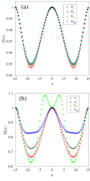
Figure 1: (Color Online) The coordinate-dependent diffusion coefficients $D_{1}$ (red diamonds), $D_{2}$(blue circles), $D_{3}$(green stars), and KP expression $D_{\rm KP}$ (black pluses) for the case studies discussed in the text. The periodicity of the channel is $\lambda=90$ ($\epsilon=0.10$) in (a) and $\lambda=30$ ($\epsilon=0.31$) in (b)

.

To further test the accuracy of the 1D effective description of the dynamics, we performed Langevin dynamics simulations of both 2D channels with a height profile $A(x)$ and a constant diffusion coefficient $D_{0}=1$ (case 1), and of 1D systems with a periodic potential $U(x)=-k_{B}T\ln\left[A\left(x\right)\right]$ and various periodic diffusion functions $D(x)$, including $D_{0}=1$ (case 2), our expressions for $D_{1}$, $D_{2}$, $D_{3}$ (cases 3-5), and $D_{\rm KP}$ (case 6). In each case, we measured the effective diffusion coefficient $D^{*}$ via Eq. (11), by simulating $5\times 10^{8}$ long trajectories of particles starting at the origin. The trajectories were computed using the G-JF integrator for Langevin’s equation of motion [21], and the spatial variations in $D(x)$ were accounted for by setting the value of the friction coefficient, $\alpha(x)=k_{B}T/D(x)$, corresponding to each time step according to the recently proposed “inertial convention” [22]. This combination (of an integrator and convention for handling the multiplicative noise) produces excellent results even for relatively large integration time steps. Our results are summarized in tables 1 and 2 which give the simulation values, along with the corresponding values derived from the MLJ formula (20) for 1D periodic systems. Table. 1 shows the results for a channel of wavelength $\lambda=90$. As can be deduced from the table, the first order diffusion coefficient $D_{1}(x)$ [Zwanzig’s expression (7)] gives remarkably precise results when compared to the 2D case. The higher order corrections, which in Fig. 1 (a) appear rather small, are unnecessary and do not yield any further improvement in the results. Furthermore, the data confirms that for slowly varying channels, The MLJ formula gives values of $D^{*}$ that are identical to the numerical counterparts (see discussion in [17]). In contrast, table 2 reveals that for $\lambda=30$, the agreement of the 1D simulations results with the 2D case is far from perfect. The first order diffusion coefficient $D_{1}$ exhibits significant improvement compared to the zeroth approximation $D_{0}$, but $D_{2}$ is no better than $D_{1}$. Both $D_{3}$ and $D_{\rm KP}$ appear to give $D^{*}$ that is quite close to the value measured in the 2D simulations, but this is clearly coincidental. Once the series expansion fails to converge (as demonstrated by the strong variations between the successive approximations exhibited in Fig 1), the accuracy of the 1D effective picture of the dynamics becomes highly questionable. The MLJ results follow the trends exhibited by their corresponding numerical values, albeit with a lesser degree of accuracy than for $\lambda=90$.

Table 1: Effective diffusion coefficients for channels with $\lambda=90$

Case studied	Simulation results	MLJ formula
(1) 2-dim	0.7340(5)	-
(2) $D_{0}$	0.7543(5)	0.7564
(3) $D_{1}$	0.7344(3)	0.7367
(4) $D_{2}$	0.7353(5)	0.7377
(5) $D_{3}$	0.7351(3)	0.7376
(6) $D_{\rm KP}$	0.7346(3)	0.7372

Table 2: Effective diffusion coefficients for channels with $\lambda=30$

Case studied	Simulation results	MLJ formula
(1) 2-dim	0.6276(3)	-
(2) $D_{0}$	0.7419(5)	0.7564
(3) $D_{1}$	0.6022(2)	0.6093
(4) $D_{2}$	0.6624(4)	0.6716
(5) $D_{3}$	0.6213(4)	0.6283
(6) $D_{\rm KP}$	0.6244(3)	0.6325

With the above said, we can clearly see from table 2 that the zeroth approximation of a constant diffusion coefficient $D(x)=D_{0}$ gives far worse results for $D^{*}$ than all the proposed expressions for coordinate-dependent $D(x)$. This observation supports Zwanzig’s idea that the modified FJ equation (6) provides a better effective 1D description of the 2D diffusion problem than the simple FJ equation (5). To further support this conclusion, we plot in fig 2 the function $\Pi(x,t)=P(x,t)A_{0}/A(x)$ for $\lambda=30$ at $t=2\times 10^{4}$. The plot shows the function $\Pi$ computed from simulations of the 2D channel (blue circles), along with those computed from 1D FJ simulations with $D_{0}$ (green stars), $D_{1}(x)=D_{\rm Z}(x)$ (Zwanzig’s formula - red diamonds), and $D_{\rm KP}(x)$ (Kalinay-Percus formula - black pluses). The degree of agreement between the function $\Pi$ of the 2D simulations and the approximations corresponding to $D_{0}$ (very poor agreement), $D_{1}$ (significantly improved agreement), and $D_{\rm KP}$ (nearly perfect agreement), is clearly in accord with the results for $D^{*}$ in table 2 showing precisely the same trends. We do not show the PDF for the higher order approximations ($D_{2}$, $D_{3}$) since, as evident from fig. 1 (b), these expressions are derived from a non-converging series expansion (see discussion in the previous paragraph). In contrast, both $D_{1}=D_{\rm Z}$ and $D_{\rm KP}$ satisfy $0<D(x)/D_{0}\leq 1$ [for any periodic function $A(x)$], which precludes strong oscillations in $D(x)$ like the ones exhibited by $D_{3}(x)$ in fig. 1 (b). We thus conclude that although the 1D projection method becomes less accurate for higher values of $\epsilon$, there is still a significant improvement in the accuracy of the PDF when $D_{1}(x)=D_{\rm Z}(x)$ and $D_{\rm KP}(x)$ are used instead of the constant $D_{0}$.

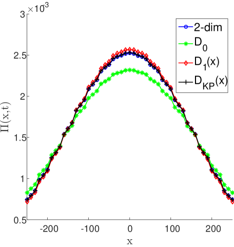
Figure 2: (Color Online) The numerical results for the function $\Pi(x,t)=P(x,t)A_{0}/A(x)$ computed from 2D channel simulation (blue circles), and from 1D FJ simulations with $D_{0}$ (green stars), $D_{1}(x)$ (red diamonds), and $D_{\rm KP}(x)$ (black pluses) for $\lambda=30$. The data is collected at $t=2\times 10^{4}$.

V Summary

In this paper we revisited the problem of describing diffusive dynamics along 2D periodic corrugated channels via a 1D FJ equation with a spatially-dependent diffusion coefficient. In contrast to previous attempts to derive expressions for $D(x)$ which were based on steady state solutions, here we consider the non-stationary state of a particle moving in an open channel. Similarly to the work in ref. [13], the expression derived here for $D(x)$ is in the form of a series expansion in the parameter $\epsilon$ associated with the aspect ratio of the channel; but in contrast to that work, the formalism presented herein does not involve complicated differnetal operators that are very hard to identify. The first order approximation, $D_{1}(x)$, coincides with Zwanzig’s formula for $D(x)$, and for long wavelength channels (small $\epsilon$) it yields results that are in perfect agreement with the 2D description. The agreement is lost when $\epsilon$ is not sufficiently small, reflecting two problems of the method. The first problem is a mathematical one: When $\epsilon$ is not small, the series expansion does not converge properly and cannot be truncated. The second problem is physical. The 1D description via FJ equation assumes a Markovian diffusion process, which is only the case in the limit of fast relaxation of the probability density in the transverese direction, i.e., for nearly flat thin channels. Therefore, one should not be surprised by the disagreement between the Langevin dynamics simulations of 1D periodic systems and the 2D simulation results for short wavelength channels. In fact, in this regime the 1D simulation results for the effective diffusion coefficient do not even agree with the Lifson-Jackson formula, which highlights yet another problem of the FJ equation - its overdamped nature. FJ is a Smoluchowski equation which is applicable only if, at length scale of the ballistic distance of the dynamics, the variations in the force associated with the entropic potential are much smaller than the characteristic friction force (see discussion in [17]) . This requirement is also not fulfilled for short wavelength channels.

As a final note, we point out that the derivation of a series expansion for $D(x)$ presented here for 2D channels can be extended to three-dimensional (3D) geometries with cylindrical symmetry. In order to do so, we assume that the 3D density, $\rho(x,r,t)$, has the same form as the 2D density (22) but with $y$ replaced by $r$, and then substitute this form in the 3D diffusion equation written in cylindrical coordinates. The resulting recurrence relation, which is different than Eq. (23) for the 2D problem, needs now to be solved, and the steps of the derivation presented in section III should be followed.

References

- [1] B. Hille, Ion Channels of Excitable Membranes (Sinauer, Sunderland, Massachusetts, 2001).
- [2] M. J. O’Connell (Ed.), Carbon Nanotubes: Properties and Applications, (CRC, Boca Raton, 2006).
- [3] A. Schüring, S. M. Auerbach, S. Fritzsche, and R. Haberlandt, J. Chem. Phys. 116, 10890 (2002).
- [4] B. H. Weigl and P. Yager, Science 283, 346 (1999).
- [5] C. Dekker, Nat. Nanotech. 2, 209 (2007).
- [6] M. H. Jacobs, Diffusion Processes (Springer, New York, 1967).
- [7] P. Sekhar Burada, G. Schmid, and P. Hänggi, Phil. Trans. R. Soc. A 367, 3157 (2009).
- [8] A. M. Berezhkovskii, L. Dagdug, and S. M. Bezrukov, J. Chem. O, J. Chem. Phys. 143, 164102 (2015).
- [9] The framework of Eq. (6) employing a local diffusion coefficient is applicable for continuous functions only, see discussion in M. Mangeat, T. Guérin and D. S. Dean, J. Chem. Phys. 149, 124105 (2018).
- [10] R. Zwanzig, J. Phys. Chem. 96, 3926 (1992).
- [11] M. Mangeat, T. Guérin and D. S. Dean, J. Stat. Mech. Theory Exp. 123205 (2017).
- [12] D. Reguera and J. M. Rubi, Phys. Rev. E 64, 061106 (2001).
- [13] P. Kalinay and J. K. Percus, Phys. Rev. E 74, 041203 (2006).
- [14] P. Kalinay and J. K. Percus, J. Chem. Phys. 122, 204701 (2005).
- [15] P. Kalinay, J. Chem. Phys. 141, 144101 (2014).
- [16] R. M. Bradley, Phys. Rev. E 80, 061142 (2009).
- [17] M. Sivan and O. Farago, Phys. Rev. E 98, 052117 (2018).
- [18] Notice that in ref. [17], we use a different notation involving the periodic function and the constant . These should be replaced here with and via the relation .
- [19] S. Lifson and J. L. Jackson, J. Chem. Phys. 36, 2410 (1962).
- [20] The scalig behavior follows from and the fact that in diffusive dynamics .
- [21] N. Grønbech-Jensen and O. Farago, Mol. Phys. 111, 983 (2013).
- [22] O. Farago and N. Grønbech-Jensen, Phys. Rev. E 89, 013301 (2014).