\WarningFilter

pstoolNo file

33footnotetext: C.M. Hackl is with the Munich University of Applied Sciences (MUAS) and head of the “Control of Renewable Energy Systems (CRES)” research group at Technical University of Munich (TUM), Germany (e-mail: christoph.hackl@hm.edu).22footnotetext: M. Landerer is with the research group “Control of renewable energy systems” (CRES) at the Munich School of Engineering (MSE), Technical University of Munich (TUM), Germany (e-mail: markus.landerer@tum.de).11footnotetext: Authors are in alphabetical order and contributed equally to the paper. Corresponding author is C.M. Hackl (christoph.hackl@hm.edu).

Modified second-order generalized integrators with modified frequency locked loop for fast harmonics estimation of distorted single-phase signals
(LONG VERSION)

C.M. Hackl‡,⋆ and M. Landerer
Abstract

This paper proposes modified Second-Order Generalized Integrators (mSOGIs) for a fast estimation of all harmonic components of arbitrarily distorted single-phase signals such as voltages or currents in power systems. The estimation is based on the internal model principle leading to an overall observer system consisting of parallelized mSOGIs. The observer is tuned by pole placement. For a constant fundamental frequency, the observer is capable of estimating all harmonic components with prescribed settling time by choosing the observer poles appropriately. For time-varying fundamental frequencies, the harmonic estimation is combined with a modified Frequency Locked Loop (mFLL) with gain normalization, sign-correct anti-windup and rate limitation. The estimation performances of the proposed parallelized mSOGIs with and without mFLL are illustrated and validated by measurement results. The results are compared to standard approaches such as parallelized standard SOGIs (sSOGIs) and adaptive notch filters (ANFs).

Index Terms:
Second-Order Generalized Integrator, Frequency Locked Loop, amplitude estimation, phase estimation, frequency estimation,

***A shorter version of this paper has been submitted to and accepted for publication in IEEE Transactions on Power Electronics (DOI: 10.1109/TPEL.2019.2932790; for more details see [1]) ***
This long version includes (i) more detailed explanations, (ii) more simulation and measurement results and (iii) a thorough theoretical analysis in its Appendix.

Notation

,,,\mathbb{N},\mathbb{R},\mathbb{C},\mathbb{Q}: natural, real, complex and rational numbers. For the following, let n,m𝑛𝑚n,m\in\mathbb{N}. 𝒙:=(x1,,xn)nassign𝒙superscriptsubscript𝑥1subscript𝑥𝑛topsuperscript𝑛\boldsymbol{x}:=(x_{1},\dots,x_{n})^{\top}\in\mathbb{R}^{n}: column vector (where :=assign:= means “is defined as” and means “transposed”). 𝟎n:=(0, 0,,,0)n\boldsymbol{0}_{n}:=(0,\,0,\,,\dots,0)^{\top}\in\mathbb{R}^{n}: zero vector. 𝟏n:=(1, 1,,,1)n\boldsymbol{1}_{n}:=(1,\,1,\,,\dots,1)^{\top}\in\mathbb{R}^{n}: vector of ones. 𝒙:=𝒙𝒙assigndelimited-∥∥𝒙superscript𝒙top𝒙\left\lVert\boldsymbol{x}\right\rVert:={\small\sqrt{\boldsymbol{x}^{\top}\boldsymbol{x}}}: Euclidean norm of 𝒙𝒙\boldsymbol{x}. 𝑨n×m𝑨superscript𝑛𝑚\boldsymbol{A}\in\mathbb{R}^{n\times m}: real (non-square) matrix. diag(𝒂)n×ndiag𝒂superscript𝑛𝑛\operatorname{diag}(\boldsymbol{a})\in\mathbb{R}^{n\times n}: diagonal matrix with diagonal entries taken from vector 𝒂=(a1,,an)n𝒂superscriptsubscript𝑎1subscript𝑎𝑛topsuperscript𝑛\boldsymbol{a}=(a_{1},\dots,a_{n})^{\top}\in\mathbb{R}^{n}. 𝑶n×mn×msubscript𝑶𝑛𝑚superscript𝑛𝑚\boldsymbol{O}_{n\times m}\in\mathbb{R}^{n\times m}: zero (non-square) matrix. 𝑰n:=diag(𝟏n)n×nassignsubscript𝑰𝑛diagsubscript1𝑛superscript𝑛𝑛\boldsymbol{I}_{n}:=\operatorname{diag}(\boldsymbol{1}_{n})\in\mathbb{R}^{n\times n}: identity matrix. blockdiag(𝑨1,,𝑨n)nm×nmblockdiagsubscript𝑨1subscript𝑨𝑛superscript𝑛𝑚𝑛𝑚\operatorname{blockdiag}(\boldsymbol{A}_{1},\dots,\boldsymbol{A}_{n})\in\mathbb{R}^{nm\times nm}: block diagonal matrix with matrix entries 𝑨im×msubscript𝑨𝑖superscript𝑚𝑚\boldsymbol{A}_{i}\in\mathbb{R}^{m\times m}, i{1,,n}𝑖1𝑛i\in\{1,\dots,n\}. χ𝑨(s):=det[s𝑰n𝑨]assignsubscript𝜒𝑨𝑠delimited-[]𝑠subscript𝑰𝑛𝑨\chi_{\boldsymbol{A}}(s):=\det[s\,\boldsymbol{I}_{n}-\boldsymbol{A}], characteristic polynomial of 𝑨n×n𝑨superscript𝑛𝑛\boldsymbol{A}\in\mathbb{R}^{n\times n}. arctan2(x,y)2𝑥𝑦\arctan\!2\big{(}x,y\big{)} 2-argument arctangent, for x,y𝑥𝑦x,y\in\mathbb{R}, defined as

arctan2:2{(0,0)}:2superscript200\displaystyle\arctan\!2\colon\mathbb{R}^{2}\setminus\{(0,0)\} \displaystyle\to (π,π],(x,y)arctan2(x,y):={arctan(yx),x>0yarctan(yx)+π,x<0y>0±π,x<0y=0arctan(yx)π,x<0y<0+π2,x=0y>0π2,x=0y<0.\displaystyle(-\pi,\pi],\quad(x,y)\mapsto\arctan\!2\big{(}x,y\big{)}:=\begin{cases}\arctan\!\big{(}\tfrac{y}{x}\big{)}&,\;x>0\wedge y\in\mathbb{R}\\ \\ \arctan\!\big{(}\tfrac{y}{x}\big{)}+\pi&,\;x<0\wedge y>0\\ \pm\pi&,\;x<0\wedge y=0\\ \arctan\!\big{(}\tfrac{y}{x}\big{)}-\pi&,\;x<0\wedge y<0\\ +\tfrac{\pi}{2}&,\;x=0\wedge y>0\\ -\tfrac{\pi}{2}&,\;x=0\wedge y<0.\\ \end{cases} (1)

I Introduction

I-A Motivation and literature review

In view of the increasing number of decentralized generation units with power electronics based grid connection and the decreasing number of large-scale generators, the overall inertia in the grid is diminishing. This results in a faster transient response and higher harmonic distortion of physical quantities (such as currents or voltages) of the power system [2]. Fast frequency fluctuations endanger stability of the power grid. Significant harmonic distortions of voltages and currents can deteriorate power quality and lead to damage or even destruction of grid components. To be capable of taking appropriate countermeasures such as (i) improving stability and quality and (ii) compensating for such deteriorated operation conditions, it is crucial to detect and estimate fundamental and higher harmonic components of the considered quantities in real time as fast and accurate as possible. Hence, grid state estimation became of particular interest to the research community in the last years and has been studied extensively (see e.g. [3, 4, 5, 6, 7, 8, 9, 10, 11, 12, 13, 14, 15, 16, 17, 18, 19, 20, 21, 22, 23, 24, 25] to name a few).

It is well known that a signal with significant harmonic distortion can be decomposed and analyzed by the Fast Fourier Transformation (FFT). However, this method requires a rather long computational time and a large amount of data to be processed [26, p. 320]. Usually, several multiples of the fundamental period (200 msabsenttimes200millisecondabsent\geq$200\text{\,}\frac{\mathrm{ms}}{}$) are needed to estimate the harmonics with acceptable accuracy [8]; when the frequency is estimated online as well, the estimation time is even longer.

The majority of the publications deals only with the estimation of fundamental signal parameters (such as amplitude and phase) and fundamental frequency. For signals with negligible harmonic distortion, several well known and rather fast methods are available [27, Chapter 4] such as Second-Order Generalized Integrator (SOGI) or Adaptive Notch Filters (ANF) with and without Phase-Locked Loop (PLL) [22] or Frequency Locked-Loop (FLL) [3, 7]. However, if the signals to be estimated have significant harmonic distortion, these approaches fail and have to be extended by the parallelization of several SOGIs (see e.g. [7, 8, 9, 14, 25]) or several ANFs (see e.g. [4, 5]); each of those being capable of estimating the individual harmonics separately. However, the resulting estimation system is highly nonlinear (in particular in combination with FLL or PLL) and difficult to tune. The estimation speed is usually faster than those of FFT approaches but still rather slow. Other estimation approaches use Adaptive Linear Kalman Filters [28], SOGIs in combination with discrete Fourier transforms [29] or circular limit cycle oscillators [30]. A comparison of estimation speed and estimation accuracy mainly focuses on fundamental signal and frequency estimation. A comparison of all the results presented in the contributions above yields that the estimation speeds vary between 401 200 ms40times1200millisecondabsent40-$1\,200\text{\,}\frac{\mathrm{ms}}{}$. The estimation speed depends on the tuning of the estimation algorithms and the operation conditions (such as changing harmonics with varying amplitudes, phases and frequencies) during the estimation process. In particular, when the frequency is changing abruptly, the overall estimation process is drastically decelerated. The FLL can be considered as the bottleneck of grid state estimation. Moreover, the performance of the parallelized estimation of the individual harmonics is mostly not discussed and evaluated.

Exceptions are the contributions [7, 8] and [4]; which explicitly discuss and show the estimation performance of the parallelized SOGIs and ANFs, respectively, for each considered harmonic component. For example, in [7], the proposed parallelized SOGIs with FLL (called MSOGI-FLL) are capable of extracting fundamental frequency and amplitudes and phases of a pre-specified number n𝑛n of harmonics ν{ν1,,νn}𝜈subscript𝜈1subscript𝜈𝑛\nu\in\{\nu_{1},\dots,\nu_{n}\}. Local stability analysis and tuning of the parallelized SOGIs and FLL were thoroughly discussed. As outcomes of the tuning rules, the gain kνsubscript𝑘𝜈k_{\nu} of the ν𝜈\nu-th SOGI should be chosen to be kν=1ν2<1ν2subscript𝑘𝜈1𝜈21𝜈2k_{\nu}=\tfrac{1}{\nu}\sqrt{2}<\tfrac{1}{\nu}2 which represents a “tradeoff between settle time, overshooting and harmonic rejection”. Simulation and measurement results were presented for three-phase signals. Six harmonics (including fundamental positive sequence) and the fundamental frequency were correctly estimated. The estimation speeds for the individual harmonics vary between 40140 ms40times140millisecondabsent40-$140\text{\,}\frac{\mathrm{ms}}{}$. Frequency estimation takes about 300 mstimes300millisecondabsent300\text{\,}\frac{\mathrm{ms}}{} to return to a constant value. In [8], a similar idea is proposed. The proposed algorithm is also based on parallelized SOGIs but a FLL has not been implemented. If the frequency is known, the method is capable of estimating the harmonics in approximately 4060 ms40times60millisecondabsent40-$60\text{\,}\frac{\mathrm{ms}}{}$111Note that, the authors state that the estimation takes less than 20 mstimes20millisecondabsent20\text{\,}\frac{\mathrm{ms}}{}, which seems not correct as can be observed in Fig. 6 and Fig. 8 in [8].. Only simulation results were presented for seven harmonics. No results were presented when the frequency is unknown and varying. Implementation and tuning of the parallelized SOGIs are hardly discussed. In [4], parallelized ANFs with FLL are implemented. For a constant (estimated) frequency, a complete stability proof for the parallelized structure is presented showing that stability is preserved if all gains are chosen positive. The parallelized ANFs with FLL are implemented in Matlab/Simulink to estimate a signal with six harmonic components (including fundamental). The fundamental frequency of the considered signal undergoes step-like changes of +4 Hztimes4hertzabsent+$4\text{\,}\frac{\mathrm{Hz}}{}$ and 2 Hztimes2hertzabsent-$2\text{\,}\frac{\mathrm{Hz}}{}$. Frequency and harmonics estimation errors tend to zero; but the estimation speed is rather slow and varies between 11,5 s1times1.5secondabsent1-$1,5\text{\,}\frac{\mathrm{s}}{}$.

As already noted, the (parallelized) SOGIs and ANFs rely on a precise estimate of the fundamental (angular) frequency for proper functionality. If the frequency is known a priori, it can be fed directly to the parallelized systems. Otherwise, the observers must be combined with a FLL (or PLL), which allows to additionally estimate the fundamental angular frequency online. Since the FLL estimation depends on the harmonic amplitudes of the input signal, [7, 17, 15] describe a Gain Normalization (GN) which robustifies the frequency estimation. Nevertheless, due to its nonlinear and time-varying dynamics, the tuning of the overall estimator consisting of parallelized SOGIs or ANFs and FLL is a non-trivial task. As a rule of thumb (coming from the steady-state derivation of the FLL adaption law), the tuning of the FLL should be slow compared to the dynamics of the parallelized SOGIs or ANFs and, therefore, significantly degrades the settling time of the overall estimation system [10]. Apart from that, negative estimates of the angular frequency lead to instability. In this context, [12] describes a saturation of the estimated angular frequency to avoid a sign change. However, this saturation does not necessarily (i) ensure convergence of the estimation error or (ii) accelerate the transient response of the FLL. In [24], the FLL is extended by output saturation and anti-windup to avoid too large estimation values. But the proposed anti-windup strategy comes with additional feedback gain (tuning parameter), which, if not properly chosen, might lead to instability. Other approaches for frequency detection are based on Phase Locked Loops (PLLs) [19], [11, 13, 21, 22] which can be combined with SOGIs as well. PLL approaches are not considered in this paper.

The remainder of this paper focuses on modifications of the parallelized “standard SOGIs” and the “standard FLL” as introduced in [3] and [7] which will allow to improve estimation speed and estimation accuracy significantly. Key observation which motivates the modifications is that almost all papers above, except [14], do only consider one single tuning factor (gain) for individual SOGI design. This single tuning factor limits the possible estimation performance. In [14], two gains are considered but their influence on the speed of harmonics estimation is not exploited and investigated. Therefore, this work proposes a modified (generalized) algorithm which achieves a prescribed settling time of the estimation process. It is capable of estimating amplitudes, angles and angular frequencies of all harmonic components of interest in real time. The proposed algorithm consists of parallelized modified SOGIs tuned by pole placement. The modified SOGIs come with additional feedback gains (additional tuning parameters) which provide the required degrees of freedom to ensure a desired (prescribed) settling time. Since the standard FLL was derived and is working for the standard SOGI only (as shown in [7] or [9]), also a modified FLL is proposed to guarantee functionality in combination with the parallelized modified SOGIs. The novelty of this paper is characterized by the following five main contributions:

  1. (i)

    Modification (generalization) of standard SOGIs (sSOGIs) to modified SOGIs (mSOGIs) with prescribed settling time (see Sections II-B and II-C);

  2. (ii)

    Parallelization of the mSOGIs and their tuning by pole placement (see Section II-D);

  3. (iii)

    Modification (generalization) of the standard FLL to the modified FLL (mFLL) with phase-correct adaption law, sign-correct anti-windup strategy and rate limitation for enhanced functionality in combination with the proposed mSOGIs (see Section III-B);

  4. (iv)

    Theoretical derivation of the pole placement algorithm and the generalized adaption law for the mFLL (see Appendix A-E and A-F,respectively);

  5. (v)

    Implementation and validation of the proposed estimation algorithm by simulation and measurement results and Comparison of the estimation performances of parallelized mSOGIs, sSOGIs and (ANFs) with and without FLL (see Section IV).

I-B Problem statement

Single-phase grid signals (e.g. voltages or currents) with significant and arbitrary harmonic distortion are considered. The considered signals are assumed to have the following form

t0:y(t):=νnaν(t)cos(ϕν(t))=:yν(t) where n:={1,ν2,,νn}>0,\forall\,t\geq 0\colon\quad y(t):=\sum\limits_{\nu\in\mathbb{H}_{n}}\underbrace{a_{\nu}(t)\cos\big{(}\phi_{\nu}(t)\big{)}}_{=:y_{\nu}(t)}\quad\text{ where }\quad\mathbb{H}_{n}:=\{1,\nu_{2},\dots,\nu_{n}\}\subset\mathbb{Q}_{>0}, (2)

with fundamental amplitude a1subscript𝑎1a_{1}, harmonic amplitudes aν2,,aνn0subscript𝑎subscript𝜈2subscript𝑎subscript𝜈𝑛0a_{\nu_{2}},\dots,a_{\nu_{n}}\geq 0 and angles ϕνsubscriptitalic-ϕ𝜈\phi_{\nu} (in radradianabsent\frac{\mathrm{rad}}{}), respectively; where νn𝜈subscript𝑛\nu\in\mathbb{H}_{n} indicates the ν𝜈\nu-th harmonic component (per definition ν1:=1assignsubscript𝜈11\nu_{1}:=1). Observe that ν𝜈\nu does not necessarily need to be a natural number or larger than one; any rational number is admissible as well (e.g. ν2=5/3subscript𝜈253\nu_{2}=5/3 or ν3=1/5subscript𝜈315\nu_{3}=1/5). Moreover, to consider the most general case, the phase angles

νnt0:ϕν(t)=0tνω(τ)dτ+ϕν,0,\forall\nu\in\mathbb{H}_{n}\;\forall t\geq 0\colon\qquad\phi_{\nu}(t)=\int_{0}^{t}\nu\,\omega\left(\tau\right)\textrm{d}\tau+\phi_{\nu,0},

of the ν𝜈\nu-th harmonic component depend on the time-varying angular fundamental frequency ω():=ω1()>0 radsassign𝜔subscript𝜔1times0radiansecond\omega(\cdot):=\omega_{1}(\cdot)>$0\text{\,}\frac{\mathrm{rad}}{\mathrm{s}}$ and the initial harmonic angle ϕν,0subscriptitalic-ϕ𝜈0\phi_{\nu,0}\in\mathbb{R}. The main goal of this paper is threefold:

  1. (i)

    to propose a modified Second-Order Generalized Integrator (mSOGI) with prescribed settling time for a fast online estimation of amplitudes a^νsubscript^𝑎𝜈\widehat{a}_{\nu} and angles ϕ^νsubscript^italic-ϕ𝜈\widehat{\phi}_{\nu}, such that, after a specified transient phase, estimated signal y^^𝑦\widehat{y} (indicated by “ ^^absent\widehat{\leavevmode\nobreak\ } ”) and original signal y𝑦y do not differ more than a given threshold εy>0subscript𝜀𝑦0\varepsilon_{y}>0. More precisely, the following should hold

    ttset:|y(t)y^(t)|εy where y^(t):=νna^ν(t)cos(ϕ^ν(t))=:y^ν(t)\forall t\geq t_{\mathrm{set}}\colon\quad|y(t)-\widehat{y}(t)|\leq\varepsilon_{y}\quad\text{ where }\quad\widehat{y}(t):=\sum\limits_{\nu\in\mathbb{H}_{n}}\underbrace{\widehat{a}_{\nu}(t)\cos\big{(}\widehat{\phi}_{\nu}(t)\big{)}}_{=:\widehat{y}_{\nu}(t)} (3)

    after a prescribed (specified) settling time tset>0 ssubscript𝑡settimes0secondabsentt_{\mathrm{set}}>$0\text{\,}\frac{\mathrm{s}}{}$;

  2. (ii)

    to propose a modified Frequency Locked Loop (mFLL) ensuring stable operation and fast estimation of the angular frequency in combination with the proposed parallelized mSOGIs; and

  3. (iii)

    to show the overall estimation performance and compare it to other standard approaches such as parallelized sSOGIs and ANFs with and without FLL.

Remark I.1.

Note that in (2), time-varying amplitudes (of each harmonic component) and time-varying angles are considered. The typical assumption (see, e.g. [27, Appendix A]) of a constant fundamental angular frequency ω>0𝜔0\omega>0 such that ϕν(t)=νωtsubscriptitalic-ϕ𝜈𝑡𝜈𝜔𝑡\phi_{\nu}(t)=\nu\omega t is not imposed, since it is not true in general.

I-C Principle idea of proposed solution

The principle idea of the proposed solution is illustrated in Fig. 1. The depicted block diagram is fed by the input signal y𝑦y to be estimated. All subsystems of the overall nonlinear observer are shown. The outputs of the block diagram are the respective estimated components of the input signal (see Sect. I-B).

Refer to caption
Figure 1: Block diagram of the nonlinear observer (consisting of parallelized mSOGIs and modified FLL (mFLL) with gain normalization (GN)).

In Fig. 1, all components (subsystems) of the nonlinear observer are explicitly shown. One can summarize: For νn𝜈subscript𝑛\nu\in\mathbb{H}_{n}, the overall nonlinear observer consists of the following subsystems:

  • a parallelization of modified Second-Order Generalized Integrators (mSOGIs) to estimate amplitude and phase of each of the harmonic components of the input signal y𝑦y. The ν𝜈\nu-th mSOGI will output the estimated state vector

    𝒙^ν:=(x^να,x^νβ)=(y^ν,q^ν)assignsubscript^𝒙𝜈superscriptsuperscriptsubscript^𝑥𝜈𝛼superscriptsubscript^𝑥𝜈𝛽topsuperscriptsubscript^𝑦𝜈subscript^𝑞𝜈top\widehat{\boldsymbol{x}}_{\nu}:=\big{(}\widehat{x}_{\nu}^{\alpha},\,\widehat{x}_{\nu}^{\beta}\big{)}^{\top}=\big{(}\widehat{y}_{\nu},\,\widehat{q}_{\nu}\big{)}^{\top}

    compromising estimates of in-phase and quadrature signals of the ν𝜈\nu-th harmonic component, i.e. y^ν=x^ναsubscript^𝑦𝜈superscriptsubscript^𝑥𝜈𝛼\widehat{y}_{\nu}=\widehat{x}_{\nu}^{\alpha} and q^ν=x^νβsubscript^𝑞𝜈superscriptsubscript^𝑥𝜈𝛽\widehat{q}_{\nu}=\widehat{x}_{\nu}^{\beta}, respectively. All n𝑛n estimated signal vectors 𝒙^νsubscript^𝒙𝜈\widehat{\boldsymbol{x}}_{\nu} are merged into the overall estimation vector

    𝒙^:=((y^1,q^1)=:𝒙^1,(y^ν2,q^ν2)=:𝒙^ν2,,(y^νn,q^νn)=:𝒙^νn)2n.assign^𝒙superscriptsubscriptsubscript^𝑦1subscript^𝑞1:absentsuperscriptsubscript^𝒙1topsubscriptsubscript^𝑦subscript𝜈2subscript^𝑞subscript𝜈2:absentsuperscriptsubscript^𝒙subscript𝜈2topsubscriptsubscript^𝑦subscript𝜈𝑛subscript^𝑞subscript𝜈𝑛:absentsuperscriptsubscript^𝒙subscript𝜈𝑛toptopsuperscript2𝑛\widehat{\boldsymbol{x}}:=\big{(}\underbrace{\left(\widehat{y}_{1},\widehat{q}_{1}\right)}_{=:\widehat{\boldsymbol{x}}_{1}^{\top}},\underbrace{\left(\widehat{y}_{\nu_{2}},\widehat{q}_{\nu_{2}}\right)}_{=:\widehat{\boldsymbol{x}}_{\nu_{2}}^{\top}},\dots,\underbrace{\left(\widehat{y}_{\nu_{n}},\widehat{q}_{\nu_{n}}\right)}_{=:\widehat{\boldsymbol{x}}_{\nu_{n}}^{\top}}\big{)}^{\top}\in\mathbb{R}^{2n}. (4)

    The output signal y^=νny^ν=𝒄𝒙^^𝑦subscript𝜈subscript𝑛subscript^𝑦𝜈superscript𝒄top^𝒙\widehat{y}=\sum_{\nu\in\mathbb{H}_{n}}\widehat{y}_{\nu}=\boldsymbol{c}^{\top}\widehat{\boldsymbol{x}} represents the estimate of the input signal y𝑦y and is established by the sum of all estimates of the in-phase signals y^ν=x^νsubscript^𝑦𝜈subscript^𝑥𝜈\widehat{y}_{\nu}=\widehat{x}_{\nu} of the mSOGIs;

  • a modified Frequency Locked Loop (mFLL) with gain normalization, generalized frequency adaption law, sign-correct anti-windup strategy and rate limitation to obtain the estimate ω^^𝜔\widehat{\omega} of the fundamental angular frequency ω𝜔\omega. The mFLL is tuned by an adaptive gain γ𝛾\gamma which depends on estimation input error ey:=yy^assignsubscript𝑒𝑦𝑦^𝑦e_{y}:=y-\widehat{y}, estimation vector 𝒙^^𝒙\widehat{\boldsymbol{x}} and estimated angular frequency ω^^𝜔\widehat{\omega};

Section II and Section III introduce the different subsystems (i.e. mSOGIs and mFLL) illustrated in Fig. 1 and explain in more detail their contribution to the proposed solution for real-time estimation of amplitudes and phases of all n𝑛n harmonics of the input signal y𝑦y as in (2) as well as the fundamental frequency ω𝜔\omega.

II Second-Order Generalized Integrators (SOGIs): In-phase and quadrature signal estimation

The key tool to estimate in-phase and quadrature signals of a measured sinusoidal signal is a Second-Order Generalized Integrator (SOGI) [27, App. A]. Their parallelization in combination with a FLL (see Sect. III) allows to detect all harmonic components and the fundamental frequency. First, a standard SOGI (as e.g. discussed in [7]) for the ν𝜈\nu-th harmonic is revisited. After that, the proposed modification to it is introduced to obtain the modified SOGI with prescribed settling time. It is shown that the modified SOGI is actually a generalization of the standard SOGI. Next, their estimation performances are compared. Finally, to be capable of estimating all n𝑛n harmonics, the proposed modified (or standard) SOGIs are parallelized to obtain the overall observer system. Throughout this paper, the more powerful state space representation will be used, since the considered parallelized SOGIs with FLL represent a nonlinear system and transfer functions are not applicable.

II-A Standard SOGI (sSOGI) for the ν𝜈\nu-th harmonic component [7]

For now, let νn𝜈subscript𝑛\nu\in\mathbb{H}_{n} and consider only the ν𝜈\nu-th harmonic component yν(t):=aν(t)cos(ϕν(t))assignsubscript𝑦𝜈𝑡subscript𝑎𝜈𝑡subscriptitalic-ϕ𝜈𝑡y_{\nu}(t):=a_{\nu}(t)\cos\!\left(\phi_{\nu}(t)\right). If the estimate ω^ν:=νω^assignsubscript^𝜔𝜈𝜈^𝜔\widehat{\omega}_{\nu}:=\nu\widehat{\omega} of the ν𝜈\nu-th harmonic frequency is known, the implementation of a sSOGI for the signal yνsubscript𝑦𝜈y_{\nu} allows to obtain online estimates y^ν=x^ναsubscript^𝑦𝜈subscriptsuperscript^𝑥𝛼𝜈\widehat{y}_{\nu}=\widehat{x}^{\alpha}_{\nu} and q^ν=x^νβsubscript^𝑞𝜈subscriptsuperscript^𝑥𝛽𝜈\widehat{q}_{\nu}=\widehat{x}^{\beta}_{\nu} of in-phase and quadrature signal, respectively. A sSOGI for the ν𝜈\nu-th harmonic component is depicted in Fig. 2 (a). Its dynamics are given by the following time-varying differential equation

ddt(x^να(t)x^νβ(t))=:𝒙^ν(t)2=ω^(t)[νkννν0]=:𝑨ν(kν)2×2𝒙^ν(t)+ω^(t)(νkν0)=:𝒍ν(kν)2yν(t),𝒙^ν(0)=𝒙^ν,02y^ν(t)=(1,0)=:𝒄ν1×2𝒙^ν(t)}casesdd𝑡superscriptmatrixsuperscriptsubscript^𝑥𝜈𝛼𝑡superscriptsubscript^𝑥𝜈𝛽𝑡:absentsubscript^𝒙𝜈𝑡absentsuperscript2^𝜔𝑡superscriptmatrix𝜈subscript𝑘𝜈𝜈𝜈0:absentsubscript𝑨𝜈subscript𝑘𝜈absentsuperscript22subscript^𝒙𝜈𝑡^𝜔𝑡superscriptmatrix𝜈subscript𝑘𝜈0:absentsubscript𝒍𝜈subscript𝑘𝜈absentsuperscript2subscript𝑦𝜈𝑡subscript^𝒙𝜈0subscript^𝒙𝜈0superscript2subscript^𝑦𝜈𝑡subscriptmatrix10:absentsuperscriptsubscript𝒄𝜈topabsentsuperscript12subscript^𝒙𝜈𝑡\left.\begin{array}[]{rcl}\tfrac{\textrm{d}}{\textrm{d}t}\overbrace{\begin{pmatrix}\widehat{x}_{\nu}^{\alpha}(t)\\ \widehat{x}_{\nu}^{\beta}(t)\end{pmatrix}}^{=:\widehat{\boldsymbol{x}}_{\nu}(t)\in\mathbb{R}^{2}}&=&\widehat{\omega}(t)\overbrace{\begin{bmatrix}-\nu k_{\nu}&-\nu\\ \nu&0\end{bmatrix}}^{=:\boldsymbol{A}_{\nu}(k_{\nu})\in\mathbb{R}^{2\times 2}}\widehat{\boldsymbol{x}}_{\nu}(t)+\widehat{\omega}(t)\overbrace{\begin{pmatrix}\nu k_{\nu}\\ 0\end{pmatrix}}^{=:\boldsymbol{l}_{\nu}(k_{\nu})\in\mathbb{R}^{2}}y_{\nu}(t),\qquad\widehat{\boldsymbol{x}}_{\nu}\left(0\right)=\widehat{\boldsymbol{x}}_{\nu,0}\in\mathbb{R}^{2}\vspace*{2ex}\\ \widehat{y}_{\nu}(t)&=&\underbrace{\begin{pmatrix}1,&0\end{pmatrix}}_{=:\boldsymbol{c}_{\nu}^{\top}\in\mathbb{R}^{1\times 2}}\widehat{\boldsymbol{x}}_{\nu}(t)\end{array}\right\} (5)

with arbitrary initial value 𝒙^ν,02subscript^𝒙𝜈0superscript2\widehat{\boldsymbol{x}}_{\nu,0}\in\mathbb{R}^{2} (mostly set to zero), gain kν>0subscript𝑘𝜈0k_{\nu}>0 (single tuning factor) and estimate ω^^𝜔\widehat{\omega} (possibly time-varying) of the fundamental angular frequency ω𝜔\omega. The gain kνsubscript𝑘𝜈k_{\nu} only allows for a limited tuning of the dynamic response of the sSOGI. For constant ω^>0^𝜔0\widehat{\omega}>0 only, characteristic equation and poles of the ν𝜈\nu-th sSOGI are given as follows222Note that for time-varying or nonlinear systems, the analysis of poles is not sufficient to check stability [31, Example 3.3.7].

χν(s):=det[s𝑰2ω^𝑨ν]=s2+νω^kνs+(νω^)2=!0pν,1/2=νω^kν2(1±14kν2).formulae-sequenceassignsubscript𝜒𝜈𝑠delimited-[]𝑠subscript𝑰2^𝜔subscript𝑨𝜈superscript𝑠2𝜈^𝜔subscript𝑘𝜈𝑠superscript𝜈^𝜔2superscript0subscript𝑝𝜈12𝜈^𝜔subscript𝑘𝜈2plus-or-minus114superscriptsubscript𝑘𝜈2\chi_{\nu}\left(s\right):=\det\left[s\boldsymbol{I}_{2}-\widehat{\omega}\boldsymbol{A}_{\nu}\right]=s^{2}+\nu\widehat{\omega}k_{\nu}\,s+(\nu\widehat{\omega})^{2}\stackrel{{\scriptstyle!}}{{=}}0\quad\Longrightarrow\quad p_{\nu,1/2}=-\frac{\nu\widehat{\omega}k_{\nu}}{2}\left(1\pm\sqrt{1-\tfrac{4}{k_{\nu}^{2}}}\right). (6)

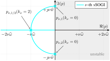
The respective root locus is shown in Fig. 2 (b). Hence, stability is guaranteed for all kν>0subscript𝑘𝜈0k_{\nu}>0. However, since the pole closest to the imaginary axis determines the settling time of the system, the smallest settling time is obtained for kν=2subscript𝑘𝜈2k_{\nu}=2 which clearly limits the tuning of the transient performance of the sSOGI. Moreover, this choice leads to two real poles at νω^kν2𝜈^𝜔subscript𝑘𝜈2-\frac{\nu\widehat{\omega}k_{\nu}}{2} and, hence, the sSOGI is not capable of oscillating by itself. Therefore, common tunings are kν=2/νsubscript𝑘𝜈2𝜈k_{\nu}=\sqrt{2}/\nu [7] or kν=1subscript𝑘𝜈1k_{\nu}=1 [4].

Refer to caption
(a) Block diagram of ν𝜈\nu-th sSOGI with one single tuning parameter kνsubscript𝑘𝜈k_{\nu}.
Refer to caption
(b) Root locus of ν𝜈\nu-th sSOGI for kν>0subscript𝑘𝜈0k_{\nu}>0 (unstable for kν<0subscript𝑘𝜈0k_{\nu}<0).
Figure 2: Standard Second-Order Generalized Integrator (sSOGI[7]: (a) Block diagram and (b) root locus of ν𝜈\nu-th sSOGI.

II-B Modified SOGI (mSOGI) for the ν𝜈\nu-th harmonic component

To overcome the problem of the limited tuning without the possibility to prescribe the settling time, the modified SOGI (mSOGI) with additional gain gνsubscript𝑔𝜈g_{\nu} is introduced. The resulting block diagram of the ν𝜈\nu-th mSOGI is illustrated in Fig. 3 (a). Note that the additional gain does not impair functionality but gives the necessary degree of freedom to enhance the transient performance as will be shown in the next subsection.

Refer to caption
(a) Block diagram of ν𝜈\nu-th mSOGI with two tuning parameters kνsubscript𝑘𝜈k_{\nu} and gνsubscript𝑔𝜈g_{\nu}.
Refer to caption
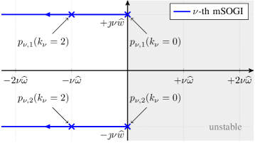
(b) Root locus of ν𝜈\nu-th mSOGI for kν>0subscript𝑘𝜈0k_{\nu}>0 and gν=kν24subscript𝑔𝜈superscriptsubscript𝑘𝜈24g_{\nu}=-\tfrac{k_{\nu}^{2}}{4} (in general unstable for kν<0subscript𝑘𝜈0k_{\nu}<0 or gν>1subscript𝑔𝜈1g_{\nu}>1).
Figure 3: Modified Second-Order Generalized Integrator (mSOGI): (a) Block diagram and (b) root locus of ν𝜈\nu-th mSOGI.

The state space representation of the ν𝜈\nu-th mSOGI is given by the following time-varying differential equation:

ddt𝒙^ν(t)=ω^(t)[νkννν(1gν)0]=:𝑨ν(kν,gν)𝒙^ν(t)+ω^(t)(νkννgν)=:𝒍ν(kν,gν)yν(t),𝒙^ν(0)=𝒙^ν,02y^ν(t)=𝒄ν𝒙^ν(t)}casesdd𝑡subscript^𝒙𝜈𝑡^𝜔𝑡superscriptmatrix𝜈subscript𝑘𝜈𝜈𝜈1subscript𝑔𝜈0:absentsubscript𝑨𝜈subscript𝑘𝜈subscript𝑔𝜈subscript^𝒙𝜈𝑡^𝜔𝑡superscriptmatrix𝜈subscript𝑘𝜈𝜈subscript𝑔𝜈:absentsubscript𝒍𝜈subscript𝑘𝜈subscript𝑔𝜈subscript𝑦𝜈𝑡subscript^𝒙𝜈0subscript^𝒙𝜈0superscript2subscript^𝑦𝜈𝑡superscriptsubscript𝒄𝜈topsubscript^𝒙𝜈𝑡\boxed{\left.\begin{array}[]{rcl}\tfrac{\textrm{d}}{\textrm{d}t}\widehat{\boldsymbol{x}}_{\nu}(t)&=&\widehat{\omega}(t)\overbrace{\begin{bmatrix}-\nu k_{\nu}&-\nu\\ \nu(1-g_{\nu})&0\end{bmatrix}}^{=:\boldsymbol{A}_{\nu}(k_{\nu},g_{\nu})}\widehat{\boldsymbol{x}}_{\nu}(t)+\widehat{\omega}(t)\overbrace{\begin{pmatrix}\nu k_{\nu}\\ \nu g_{\nu}\end{pmatrix}}^{=:\boldsymbol{l}_{\nu}(k_{\nu},g_{\nu})}y_{\nu}(t),\qquad\widehat{\boldsymbol{x}}_{\nu}\left(0\right)=\widehat{\boldsymbol{x}}_{\nu,0}\in\mathbb{R}^{2}\\[8.61108pt] \widehat{y}_{\nu}(t)&=&\boldsymbol{c}_{\nu}^{\top}\widehat{\boldsymbol{x}}_{\nu}(t)\end{array}\right\}} (7)

with arbitrary initial value 𝒙^ν,02subscript^𝒙𝜈0superscript2\widehat{\boldsymbol{x}}_{\nu,0}\in\mathbb{R}^{2} and estimate ω^^𝜔\widehat{\omega} of ω𝜔\omega. The gains kνsubscript𝑘𝜈k_{\nu} and gνsubscript𝑔𝜈g_{\nu} now allow (theoretically333Of course, noise will limit the feasible tuning.) for a limitless tuning of the dynamic response of the mSOGI. The tiny but crucial difference between the mSOGI in (7) and the sSOGI in (5) is the additional gain gνsubscript𝑔𝜈g_{\nu} in the system matrix 𝑨ν(kν,gν)subscript𝑨𝜈subscript𝑘𝜈subscript𝑔𝜈\boldsymbol{A}_{\nu}(k_{\nu},g_{\nu}) and the vector 𝒍ν(kν,gν)subscript𝒍𝜈subscript𝑘𝜈subscript𝑔𝜈\boldsymbol{l}_{\nu}(k_{\nu},g_{\nu}). For a constant frequency ω^^𝜔\widehat{\omega}, the characteristic equation and the poles of the ν𝜈\nu-th mSOGI are given by

χν(s):=det[s𝑰2ω^𝑨ν]=s2+νω^kνs+(1gν)(νω^)2=!0assignsubscript𝜒𝜈𝑠delimited-[]𝑠subscript𝑰2^𝜔subscript𝑨𝜈superscript𝑠2𝜈^𝜔subscript𝑘𝜈𝑠1subscript𝑔𝜈superscript𝜈^𝜔2superscript0\displaystyle\chi_{\nu}\left(s\right):=\det\left[s\boldsymbol{I}_{2}-\widehat{\omega}\boldsymbol{A}_{\nu}\right]=s^{2}+\nu\widehat{\omega}k_{\nu}s+\left(1-g_{\nu}\right)(\nu\widehat{\omega})^{2}\stackrel{{\scriptstyle!}}{{=}}0 \displaystyle\Longrightarrow pν,1/2=νω^kν2(1±14(1gν)kν2)subscript𝑝𝜈12𝜈^𝜔subscript𝑘𝜈2plus-or-minus1141subscript𝑔𝜈superscriptsubscript𝑘𝜈2\displaystyle p_{\nu,1/2}=-\tfrac{\nu\widehat{\omega}k_{\nu}}{2}\left(1\pm\sqrt{1-4\tfrac{(1-g_{\nu})}{k_{\nu}^{2}}}\right) (8)
gν=kν24superscriptsubscript𝑔𝜈superscriptsubscript𝑘𝜈24\displaystyle\stackrel{{\scriptstyle g_{\nu}=-\tfrac{k_{\nu}^{2}}{4}}}{{\Longrightarrow}} pν,1/2=νω^kν2±ȷνω^.subscript𝑝𝜈12plus-or-minus𝜈^𝜔subscript𝑘𝜈2italic-ȷ𝜈^𝜔\displaystyle p_{\nu,1/2}=-\tfrac{\nu\widehat{\omega}k_{\nu}}{2}\pm\jmath\nu\widehat{\omega}.

The special choice of the additional gain gν=kν24subscript𝑔𝜈superscriptsubscript𝑘𝜈24g_{\nu}=-\tfrac{k_{\nu}^{2}}{4} in (8) gives the key feature of the mSOGI: For any kν>0subscript𝑘𝜈0k_{\nu}>0, the real parts of the poles pν,1/2subscript𝑝𝜈12p_{\nu,1/2} in (8) can be chosen arbitrarily; whereas the capability of the mSOGI to oscillate with angular frequency νω^𝜈^𝜔\nu\widehat{\omega} is preserved (see imaginary parts of pν,1/2subscript𝑝𝜈12p_{\nu,1/2}). The root locus of the ν𝜈\nu-th mSOGI is depicted in Fig. 3 (b). The mSOGI is stable for any kν>0subscript𝑘𝜈0k_{\nu}>0; and, the larger kνsubscript𝑘𝜈k_{\nu} is chosen, the faster is its transient response.

Remark II.1 (Generaliziation of the sSOGI).

The introduction of the additional gain gνsubscript𝑔𝜈g_{\nu} for the mSOGI in (7) represents actually a generalization of the sSOGI in (5). Clearly, for gν=0subscript𝑔𝜈0g_{\nu}=0, the mSOGI simplifies to the sSOGI. In other words, only now, the term “second-order generalized integrator” is really appropriate.

II-C Comparison of the estimation performances of sSOGI and mSOGI

If ω^=ω^𝜔𝜔\widehat{\omega}=\omega, both SOGIs are capable of estimating in-phase signal y^ν=x^ναsubscript^𝑦𝜈subscriptsuperscript^𝑥𝛼𝜈\widehat{y}_{\nu}=\widehat{x}^{\alpha}_{\nu} and quadrature signal q^ν=x^νβsubscript^𝑞𝜈subscriptsuperscript^𝑥𝛽𝜈\widehat{q}_{\nu}=\widehat{x}^{\beta}_{\nu} of the ν𝜈\nu-th harmonic signal yν(t):=aν(t)cos(ϕν(t))assignsubscript𝑦𝜈𝑡subscript𝑎𝜈𝑡subscriptitalic-ϕ𝜈𝑡y_{\nu}(t):=a_{\nu}(t)\cos\!\left(\phi_{\nu}(t)\right). The estimated amplitude

a^ν(t):=𝒙^ν(t)=y^ν(t)2+q^ν(t)2assignsubscript^𝑎𝜈𝑡delimited-∥∥subscript^𝒙𝜈𝑡subscript^𝑦𝜈superscript𝑡2subscript^𝑞𝜈superscript𝑡2\widehat{a}_{\nu}(t):=\left\lVert\widehat{\boldsymbol{x}}_{\nu}(t)\right\rVert=\sqrt{\widehat{y}_{\nu}(t)^{2}+\widehat{q}_{\nu}(t)^{2}} (9)

is given by the norm of the estimated signal and its quadrature signal. The estimated phase angle is given by

ϕ^ν(t)=arctan2(y^ν(t),q^ν(t)) with arctan2(,) as in (1).subscript^italic-ϕ𝜈𝑡2subscript^𝑦𝜈𝑡subscript^𝑞𝜈𝑡 with 2 as in italic-(1italic-)\widehat{\phi}_{\nu}(t)=\arctan\!2\big{(}\widehat{y}_{\nu}(t),\,\widehat{q}_{\nu}(t)\big{)}\quad\text{ with }\quad\arctan\!2(\cdot,\cdot)\text{ as in }\eqref{eq:[N]definition of atan2}. (10)

Hence, the parameters a^νsubscript^𝑎𝜈\widehat{a}_{\nu} and ϕ^νsubscript^italic-ϕ𝜈\widehat{\phi}_{\nu} of the ν𝜈\nu-th harmonic can be detected online.

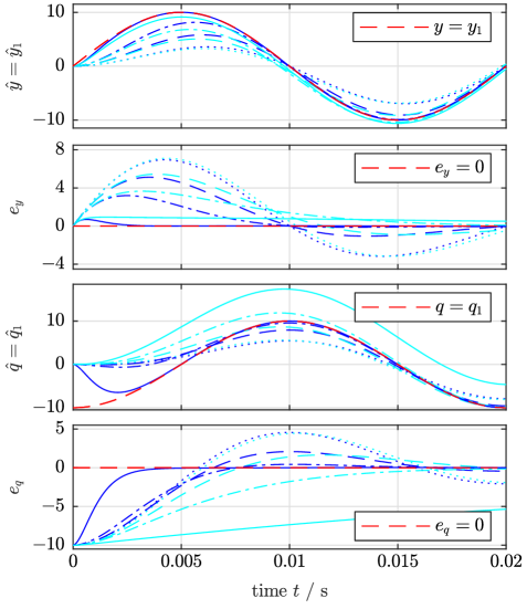
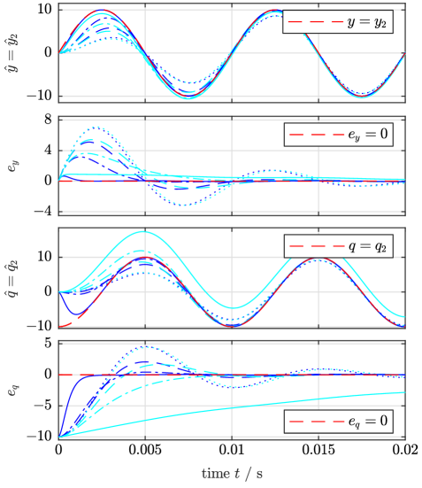
In Fig. 4, the transient responses of sSOGI and mSOGI are shown in cyan and blue, respectively, for the first harmonic (i.e. ν=1𝜈1\nu=1, see Fig. 4(a)) and for second harmonic (i.e. ν=2𝜈2\nu=2, see Fig. 4(b)). Four tunings of the gain kνsubscript𝑘𝜈k_{\nu} are implemented and illustrated by different line types: kν=0.5subscript𝑘𝜈0.5k_{\nu}=0.5 (dotted), kν=1subscript𝑘𝜈1k_{\nu}=1 (dashed), kν=2subscript𝑘𝜈2k_{\nu}=2 (dash-dotted) and kν=10subscript𝑘𝜈10k_{\nu}=10 (solid). The larger kνsubscript𝑘𝜈k_{\nu} is chosen, the faster is the transient response of the mSOGI. Moreover, for kν=2subscript𝑘𝜈2k_{\nu}=2 (dash-dotted) or kν=10subscript𝑘𝜈10k_{\nu}=10 (solid), settling times of e.g. tset=0,01 ssubscript𝑡settimes0.01secondabsentt_{\mathrm{set}}=$0,01\text{\,}\frac{\mathrm{s}}{}$ and tset=0,005 ssubscript𝑡settimes0.005secondabsentt_{\mathrm{set}}=$0,005\text{\,}\frac{\mathrm{s}}{}$ can be guaranteed for the fundamental signal, respectively. For the second harmonic, the transient response is twice as fast as for the fundamental signal. For the sSOGI, a prescribed settling time cannot be ensured, since one pole approaches the imaginary axis for large choices of kνsubscript𝑘𝜈k_{\nu} (see also Fig. 2). In particular, the estimation of the quadrature component is slow (see eqsubscript𝑒𝑞e_{q} in Fig. 4) which degrades the estimation speed of positive, negative and zero sequences in three-phase systems (not considered in this paper).
Refer to caption
(a) Estimation of fundamental component of first harmonic (ν=1𝜈1\nu=1).
Refer to caption
(b) Estimation of second harmonic component (ν=2𝜈2\nu=2).
Figure 4: Comparison of estimation performances of ν𝜈\nu-th sSOGI ( , , , ) and ν𝜈\nu-th mSOGI ( , , , ) for four different tunings of gain kν{0.5,1,2,10}subscript𝑘𝜈0.51210k_{\nu}\in\{0.5,1,2,10\}, respectively. Signals shown in (a) for ν=1𝜈1\nu=1 and in (b) for ν=2𝜈2\nu=2 are from top to bottom: input signal yνsubscript𝑦𝜈y_{\nu} and its estimate y^νsubscript^𝑦𝜈\widehat{y}_{\nu}, estimation in-phase error ey=yνy^νsubscript𝑒𝑦subscript𝑦𝜈subscript^𝑦𝜈e_{y}=y_{\nu}-\widehat{y}_{\nu}, quadrature signal qνsubscript𝑞𝜈q_{\nu} and its estimate q^νsubscript^𝑞𝜈\widehat{q}_{\nu} and estimation quadrature error eq=qνq^νsubscript𝑒𝑞subscript𝑞𝜈subscript^𝑞𝜈e_{q}=q_{\nu}-\widehat{q}_{\nu}

II-D Parallelization of the mSOGIs

This far, the presented SOGIs (sSOGIs and mSOGIs) can only estimate in-phase signal y^ν=x^ναsubscript^𝑦𝜈subscriptsuperscript^𝑥𝛼𝜈\widehat{y}_{\nu}=\widehat{x}^{\alpha}_{\nu} and quadrature signal q^ν=x^νβsubscript^𝑞𝜈subscriptsuperscript^𝑥𝛽𝜈\widehat{q}_{\nu}=\widehat{x}^{\beta}_{\nu} of the ν𝜈\nu-th harmonic signal yν(t):=aν(t)cos(ϕν(t))assignsubscript𝑦𝜈𝑡subscript𝑎𝜈𝑡subscriptitalic-ϕ𝜈𝑡y_{\nu}(t):=a_{\nu}(t)\cos\!\left(\phi_{\nu}(t)\right). By parallelizing n𝑛n of the mSOGIs or sSOGIs (see Fig. 1), it is possible to extract in-phase and quadrature signal of each harmonic component yνsubscript𝑦𝜈y_{\nu} for all νn𝜈subscript𝑛\nu\in\mathbb{H}_{n}. For the parallelized sSOGIs, stability is preserved for a positive choice of all gains, i.e. kν>0subscript𝑘𝜈0k_{\nu}>0 for all νn𝜈subscript𝑛\nu\in\mathbb{H}_{n} [4]. Stability for the parallelized mSOGIs will be guaranteed by pole placement. Moreover, the settling time can only be pre-specified by the parallelized mSOGIs.

The idea of the parallelization can be motivated by recalling the internal model principle which states that "[e]very good regulator [or observer] must incorporate a model of the outside world being capable to reduplicate the dynamic structure of the exogenous signals which the regulator [or observer] is required to process." [32]. In the considered case, the exogenous signal y𝑦y as in (2) can be reduplicated by the parallelization of n𝑛n sinusoidal internal models [33, Chapter 20], which have the overall dynamics

ddt𝒙(t)=ω(t)𝑱𝒙(t),𝒙(0)=𝒙0𝟎2n2ny(t)=(1, 0, 1, 0,, 1, 0)=:𝒄2n𝒙(t)}\left.\begin{array}[]{rcl}\tfrac{\textrm{d}}{\textrm{d}t}\boldsymbol{x}(t)&=&\omega(t)\boldsymbol{J}\boldsymbol{x}(t),\qquad\qquad\qquad\qquad\boldsymbol{x}\left(0\right)=\boldsymbol{x}_{0}\neq\boldsymbol{0}_{2n}\in\mathbb{R}^{2n}\vspace*{1ex}\\ y(t)&=&\underbrace{(1,\,0,\,1,\,0,\,\cdots,\,1,\,0)}_{=:\,\boldsymbol{c}^{\top}\in\mathbb{R}^{2n}}\boldsymbol{x}(t)\end{array}\qquad\right\} (11)

where

𝒙:=((x1α,x1β)=:𝒙1,,𝒙n),𝑱:=blockdiag(𝑱¯,ν2𝑱¯,,νn𝑱¯)2n×2n and 𝑱¯=[0110]=𝑱¯=𝑱¯1.\boldsymbol{x}:=\big{(}(\underbrace{x_{1}^{\alpha},\,x_{1}^{\beta})}_{=:\boldsymbol{x}_{1}^{\top}},\,\ldots,\,\boldsymbol{x}_{n}^{\top}\big{)}^{\top},\;\boldsymbol{J}:=\operatorname{blockdiag}\left(\overline{\boldsymbol{J}},\nu_{2}\overline{\boldsymbol{J}},\cdots,\nu_{n}\overline{\boldsymbol{J}}\right)\in\mathbb{R}^{2n\times 2n}\;\text{ and }\;\overline{\boldsymbol{J}}=\begin{bmatrix}0&-1\\ 1&0\end{bmatrix}=-\overline{\boldsymbol{J}}^{\top}=-\overline{\boldsymbol{J}}^{-1}. (12)

The initial values of the internal model in (11) allow to determine amplitude aνsubscript𝑎𝜈a_{\nu} and angle ϕνsubscriptitalic-ϕ𝜈\phi_{\nu} of the ν𝜈\nu-th harmonic. For constant ω>0𝜔0\omega>0 and differing harmonics νiνjsubscript𝜈𝑖subscript𝜈𝑗\nu_{i}\neq\nu_{j} for all ij{1,n}𝑖𝑗1𝑛i\neq j\in\{1,\dots n\}, the overall internal model (11) is completely state observable (see Proposition A.1 in the appendix).

Now, by substituting estimate ω^^𝜔\widehat{\omega} for ω𝜔\omega, the observer is obtained and consists of the parallelized mSOGIs (as introduced in (7) for the ν𝜈\nu-th harmonic). The observer dynamics are nonlinear and given by

ddt𝒙^(t)=ω^(t)𝑱𝒙^(t)+ω^(t)𝒍(y(t)𝒄𝒙^(t)=y^(t))=ω^(t)[𝑱𝒍𝒄=:𝑨]𝒙^(t)+ω^(t)𝒍y(t),𝒙^(t)=𝒙^02ny^(t)=(𝒄1,𝒄ν2,,𝒄νn)=(11),(7)𝒄𝒙^(t),}casesdd𝑡^𝒙𝑡^𝜔𝑡𝑱^𝒙𝑡^𝜔𝑡𝒍𝑦𝑡superscriptsuperscript𝒄top^𝒙𝑡absent^𝑦𝑡missing-subexpression^𝜔𝑡delimited-[]subscript𝑱𝒍superscript𝒄top:absent𝑨^𝒙𝑡^𝜔𝑡𝒍𝑦𝑡^𝒙𝑡subscript^𝒙0superscript2𝑛^𝑦𝑡subscriptsuperscriptsubscript𝒄1topsuperscriptsubscript𝒄subscript𝜈2topsuperscriptsubscript𝒄subscript𝜈𝑛topsuperscriptitalic-(11italic-)italic-(7italic-)absentsuperscript𝒄top^𝒙𝑡\boxed{\left.\begin{array}[]{rcl}\tfrac{\textrm{d}}{\textrm{d}t}\widehat{\boldsymbol{x}}(t)&=&\widehat{\omega}(t)\boldsymbol{J}\widehat{\boldsymbol{x}}(t)+\widehat{\omega}(t)\,\boldsymbol{l}\,\big{(}y(t)-\overbrace{\boldsymbol{c}^{\top}\widehat{\boldsymbol{x}}(t)}^{=\widehat{y}(t)}\big{)}\vspace*{1ex}\\ &=&\widehat{\omega}(t)\big{[}\underbrace{\boldsymbol{J}-\boldsymbol{l}\boldsymbol{c}^{\top}}_{=:\boldsymbol{A}}\big{]}\widehat{\boldsymbol{x}}(t)+\widehat{\omega}(t)\,\boldsymbol{l}\,y(t),\qquad\qquad\widehat{\boldsymbol{x}}(t)=\widehat{\boldsymbol{x}}_{0}\in\mathbb{R}^{2n}\vspace*{2ex}\\ \widehat{y}(t)&=&\underbrace{\big{(}\boldsymbol{c}_{1}^{\top},\boldsymbol{c}_{\nu_{2}}^{\top},\cdots,\boldsymbol{c}_{\nu_{n}}^{\top}\big{)}}_{\stackrel{{\scriptstyle\eqref{eq:state space dynamics of overall IM},\eqref{eq:esogi_state_space}}}{{=}}\boldsymbol{c}^{\top}}\widehat{\boldsymbol{x}}(t),\end{array}\right\}} (13)

where observer state vector 𝒙^=(7)(𝒙^1,𝒙^ν2,,𝒙^νn)2nsuperscriptitalic-(7italic-)^𝒙superscriptsuperscriptsubscript^𝒙1topsuperscriptsubscript^𝒙subscript𝜈2topsuperscriptsubscript^𝒙subscript𝜈𝑛toptopsuperscript2𝑛\widehat{\boldsymbol{x}}\stackrel{{\scriptstyle\eqref{eq:esogi_state_space}}}{{=}}\big{(}\widehat{\boldsymbol{x}}_{1}^{\top},\widehat{\boldsymbol{x}}_{\nu_{2}}^{\top},\cdots,\widehat{\boldsymbol{x}}_{\nu_{n}}^{\top}\big{)}^{\top}\in\mathbb{R}^{2n} and observer gain vector

𝒍:=(𝒍1,𝒍ν2,,𝒍νn)=(7)(k1,g1,,νnkn,νngn)2nassign𝒍superscriptsuperscriptsubscript𝒍1topsuperscriptsubscript𝒍subscript𝜈2topsuperscriptsubscript𝒍subscript𝜈𝑛toptopsuperscriptitalic-(7italic-)superscriptsubscript𝑘1subscript𝑔1subscript𝜈𝑛subscript𝑘𝑛subscript𝜈𝑛subscript𝑔𝑛topsuperscript2𝑛\boldsymbol{l}:=\big{(}\boldsymbol{l}_{1}^{\top},\boldsymbol{l}_{\nu_{2}}^{\top},\cdots,\boldsymbol{l}_{\nu_{n}}^{\top}\big{)}^{\top}\stackrel{{\scriptstyle\eqref{eq:esogi_state_space}}}{{=}}\left(k_{1},\,g_{1},\,\ldots,\,\nu_{n}k_{n},\,\nu_{n}g_{n}\right)^{\top}\in\mathbb{R}^{2n} (14)

merge the individual sub-state estimation vectors 𝒙^νsubscript^𝒙𝜈\widehat{\boldsymbol{x}}_{\nu} and gain vectors 𝒍νsubscript𝒍𝜈\boldsymbol{l}_{\nu} of the ν𝜈\nu mSOGIs as in (7). The observer will be tuned by pole placement and, hence, the gains in 𝒍𝒍\boldsymbol{l} can be determined by comparing the coefficients of the characteristic polynomial

χ𝑨(s)=i=1n(s2+νi2)i=1ngiνi2k=1kin(s2+νk2)+si=1nkiνik=1kin(s2+νk2)subscript𝜒𝑨𝑠superscriptsubscriptproduct𝑖1𝑛superscript𝑠2superscriptsubscript𝜈𝑖2superscriptsubscript𝑖1𝑛subscript𝑔𝑖superscriptsubscript𝜈𝑖2superscriptsubscriptproduct𝑘1𝑘𝑖𝑛superscript𝑠2superscriptsubscript𝜈𝑘2𝑠superscriptsubscript𝑖1𝑛subscript𝑘𝑖subscript𝜈𝑖superscriptsubscriptproduct𝑘1𝑘𝑖𝑛superscript𝑠2superscriptsubscript𝜈𝑘2\chi_{\boldsymbol{A}}\left(s\right)=\prod\limits_{i=1}^{n}\left(s^{2}+\nu_{i}^{2}\right)-\sum\limits_{i=1}^{n}g_{i}\nu_{i}^{2}\prod\limits_{\begin{subarray}{c}k=1\\ k\neq i\end{subarray}}^{n}\left(s^{2}+\nu_{k}^{2}\right)+s\sum\limits_{i=1}^{n}k_{i}\nu_{i}\prod\limits_{\begin{subarray}{c}k=1\\ k\neq i\end{subarray}}^{n}\left(s^{2}+\nu_{k}^{2}\right) (15)

of the closed-loop system matrix 𝑨:=𝑱𝒍𝒄assign𝑨𝑱𝒍superscript𝒄top\boldsymbol{A}:=\boldsymbol{J}-\boldsymbol{l}\boldsymbol{c}^{\top} in (13) and the coefficients of a desired polynomial

χ𝑨(s):=i=12n(spi)assignsuperscriptsubscript𝜒𝑨𝑠superscriptsubscriptproduct𝑖12𝑛𝑠superscriptsubscript𝑝𝑖\chi_{\boldsymbol{A}}^{*}\left(s\right):=\prod\limits_{i=1}^{2n}\left(s-p_{i}^{*}\right) (16)

with 2n2𝑛2n prescribed stable roots (poles) pi<0superscriptsubscript𝑝𝑖subscriptabsent0p_{i}^{*}\in\mathbb{C}_{<0}, i{1,,2n}𝑖12𝑛i\in\{1,\dots,2n\}, in the negative complex half-plane. The detailed derivation of the analytical solution of the pole placement algorithm is presented in Appendix A-E. The resulting feedback gain vector 𝒍𝒍\boldsymbol{l} is obtain as follows

𝒍=𝑺𝒑~𝑨,\boxed{\boldsymbol{l}=\boldsymbol{S}\,\widetilde{\boldsymbol{p}}_{\boldsymbol{A}}^{*},} (17)

where

𝑺:=[𝑺1,1𝑺n,1𝑺1,n𝑺n,n],𝑺c,r:=(1)c+1νr2(nc)𝑹ri=1irn(νr2νi2)1and𝑹i:=[1001νi]formulae-sequenceassign𝑺matrixsubscript𝑺11subscript𝑺𝑛1subscript𝑺1𝑛subscript𝑺𝑛𝑛formulae-sequenceassignsubscript𝑺𝑐𝑟superscript1𝑐1superscriptsubscript𝜈𝑟2𝑛𝑐subscript𝑹𝑟superscriptsubscriptproduct𝑖1𝑖𝑟𝑛superscriptsuperscriptsubscript𝜈𝑟2superscriptsubscript𝜈𝑖21andassignsubscript𝑹𝑖matrix1001subscript𝜈𝑖\boldsymbol{S}:=\begin{bmatrix}\boldsymbol{S}_{1,1}&\cdots&\boldsymbol{S}_{n,1}\\ \vdots&\ddots&\vdots\\ \boldsymbol{S}_{1,n}&\cdots&\boldsymbol{S}_{n,n}\end{bmatrix},\quad\boldsymbol{S}_{c,r}:=\left(-1\right)^{c+1}\nu_{r}^{2\left(n-c\right)}\boldsymbol{R}_{r}\prod\limits_{\begin{subarray}{c}i=1\\ i\neq r\end{subarray}}^{n}\left(\nu_{r}^{2}-\nu_{i}^{2}\right)^{-1}\quad\text{and}\quad\boldsymbol{R}_{i}:=\begin{bmatrix}1&0\\ 0&-\tfrac{1}{\nu_{i}}\end{bmatrix} (18)

and

𝒑~𝑨:=(i=12npi,i=12npij=i+12nsji=1nνi2,i=12npij=i+12npjk=j+12npk,,i=12npii=1nνi2).assignsuperscriptsubscript~𝒑𝑨superscriptsuperscriptsubscript𝑖12𝑛superscriptsubscript𝑝𝑖superscriptsubscript𝑖12𝑛superscriptsubscript𝑝𝑖superscriptsubscript𝑗𝑖12𝑛subscript𝑠𝑗superscriptsubscript𝑖1𝑛superscriptsubscript𝜈𝑖2superscriptsubscript𝑖12𝑛superscriptsubscript𝑝𝑖superscriptsubscript𝑗𝑖12𝑛superscriptsubscript𝑝𝑗superscriptsubscript𝑘𝑗12𝑛superscriptsubscript𝑝𝑘superscriptsubscriptproduct𝑖12𝑛superscriptsubscript𝑝𝑖superscriptsubscriptproduct𝑖1𝑛superscriptsubscript𝜈𝑖2top\widetilde{\boldsymbol{p}}_{\boldsymbol{A}}^{*}:=\left(-\sum\limits_{i=1}^{2n}p_{i}^{*},\;\;\sum\limits_{i=1}^{2n}p_{i}^{*}\sum\limits_{j=i+1}^{2n}s_{j}-\sum\limits_{i=1}^{n}\nu_{i}^{2},\;\;-\sum\limits_{i=1}^{2n}p_{i}^{*}\sum\limits_{j=i+1}^{2n}p_{j}^{*}\sum\limits_{k=j+1}^{2n}p_{k}^{*},\;\;\ldots,\;\;\prod\limits_{i=1}^{2n}p_{i}^{*}-\prod\limits_{i=1}^{n}\nu_{i}^{2}\right)^{\top}. (19)

It can be shown that, for any positive (but possibly time-varying) angular frequency estimate ω^(t)εω>0^𝜔𝑡subscript𝜀𝜔0\widehat{\omega}(t)\geq\varepsilon_{\omega}>0 for all t0𝑡0t\geq 0, the closed-loop observer system (13) is bounded-input bounded-output (BIBO) stable and input-to-state stable (ISS). Moreover, if ω^ω^𝜔𝜔\widehat{\omega}\to\omega, then the estimation state error 𝒆x:=𝒙𝒙^𝟎2nassignsubscript𝒆𝑥𝒙^𝒙subscript02𝑛\boldsymbol{e}_{x}:=\boldsymbol{x}-\widehat{\boldsymbol{x}}\to\boldsymbol{0}_{2n} decays exponentially to zero (see Theorem A.2, Theorem A.3 and Remark A.4 in the appendix).

Remark II.2 (place command in Matlab versus analytical expression in (17)).

For small n𝑛n (e.g. n10𝑛10n\leq 10), the Matlab command place can be used to compute 𝐥=place(𝐉,𝐜,)𝐥placesuperscript𝐉𝐜\boldsymbol{l}=\texttt{place}(\boldsymbol{J}^{\prime},\boldsymbol{c},\dots). For large n𝑛n, place might not provide a proper result. Moreover, place cannot place poles with multiplicity greater than rank(𝐜)=1rank𝐜1\operatorname{rank}\left(\boldsymbol{c}\right)=1. That is why, the analytical expression in (17) has been derived. It can be used to achieve pole placement for arbitrarily large n𝑛n.

III Frequency-Locked Loop (FLL): Frequency estimation

As mentioned above, a correct estimate of the fundamental angular frequency is essential for a proper functionality of the parallelized SOGIs and the harmonics detection. The following subsections motivate and discuss the necessary modifications of the FLL to ensure its functionality also with the parallelized mSOGIs.

III-A Standard FLL (sFLL) [7]

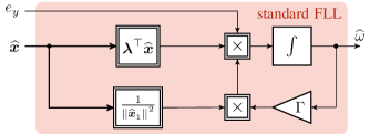
In this subsection, the standard FLL is re-visited. Its block diagram is shown in Fig. 5. Adaption law and gain normalization are briefly explained.
Refer to caption
Figure 5: Block diagram of standard Frequency Locked Loop (sFLL) with gain normalization [4, 7, 17].

III-A1 Adaption law

As shown in Fig. 1, any of the n𝑛n parallelized mSOGIs requires an estimate ω^^𝜔\widehat{\omega} of the fundamental angular frequency ω𝜔\omega. The estimate ω^^𝜔\widehat{\omega} is the output of the FLL. The nonlinear adaption law of the sFLL is given by [7]

ddtω^(t)=γ(t)𝝀𝒙^(t)ey(t)=[4]γ(t)k1x^1β(t)ey(t),ω^(0)=ω^0,formulae-sequencedd𝑡^𝜔𝑡𝛾𝑡superscript𝝀top^𝒙𝑡subscript𝑒𝑦𝑡superscript[4]𝛾𝑡subscript𝑘1superscriptsubscript^𝑥1𝛽𝑡subscript𝑒𝑦𝑡^𝜔0subscript^𝜔0\tfrac{\textrm{d}}{\textrm{d}t}\widehat{\omega}(t)=\gamma(t)\boldsymbol{\lambda}^{\top}\widehat{\boldsymbol{x}}(t)e_{y}(t)\stackrel{{\scriptstyle\text{\cite[cite]{[\@@bibref{}{2007_Mojiri_Time-DomainSignalAnalysisUsingAdaptiveNotchFilter}{}{}]}}}}{{=}}\gamma(t)\,k_{1}\,\widehat{x}_{1}^{\beta}(t)\,e_{y}(t),\qquad\widehat{\omega}(0)=\widehat{\omega}_{0}\in\mathbb{R}, (20)

where γ()>0𝛾0\gamma(\cdot)>0 is a positive but non-constant adaptive gain, 𝝀=(0,k1,𝟎2n2)𝝀superscript0subscript𝑘1superscriptsubscript02𝑛2toptop\boldsymbol{\lambda}=(0,-k_{1},\boldsymbol{0}_{2n-2}^{\top})^{\top} [4, 7] is a constant "selection" vector (to extract only the fundamental estimate x^1βsuperscriptsubscript^𝑥1𝛽\widehat{x}_{1}^{\beta} from 𝒙^^𝒙\widehat{\boldsymbol{x}}), 𝒙^^𝒙\widehat{\boldsymbol{x}} is the estimation vector of the parallelized sSOGIs and ey:=yy^assignsubscript𝑒𝑦𝑦^𝑦e_{y}:=y-\widehat{y} is the estimation error (difference between input y𝑦y and estimated input y^^𝑦\widehat{y}). A proper choice of the initial value, e.g. ω^0{2π 50,2π 60}subscript^𝜔02𝜋502𝜋60\widehat{\omega}_{0}\in\{2\pi\,50,2\pi\,60\}, of the sFLL adaption law is beneficial for functionality and adaption speed.

Remark III.1 (Impact of negative estimates of the angular frequency).

Note that, in view of the adaption law in (20), the estimated angular frequency might also become negative, i.e. ω^(τ)<0^𝜔𝜏0\widehat{\omega}(\tau)<0 for some time instant τ0𝜏0\tau\geq 0. However, a negative ω^<0^𝜔0\widehat{\omega}<0 will result in instability of the parallelized sSOGIs and all estimated states will diverge.

III-A2 Gain Normalization (GN)

The FLL should be robustified to work for signals with arbitrary fundamental amplitudes and angular frequencies (see [7, 17]). This can be achieved by introducing the following adaptive sFLL gain

γ(t):=Γω^(t)𝒙^1(t)2ddtω^=Γω^(t)𝒙^1(t)2k1x^1β(t)ey(t),formulae-sequenceassign𝛾𝑡Γ^𝜔𝑡superscriptdelimited-∥∥subscript^𝒙1𝑡2dd𝑡^𝜔Γ^𝜔𝑡superscriptdelimited-∥∥subscript^𝒙1𝑡2subscript𝑘1superscriptsubscript^𝑥1𝛽𝑡subscript𝑒𝑦𝑡\gamma(t):=\Gamma\tfrac{\widehat{\omega}(t)}{\left\lVert\widehat{\boldsymbol{x}}_{1}(t)\right\rVert^{2}}\qquad\Longrightarrow\qquad\tfrac{\textrm{d}}{\textrm{d}t}\widehat{\omega}=\Gamma\tfrac{\widehat{\omega}(t)}{\left\lVert\widehat{\boldsymbol{x}}_{1}(t)\right\rVert^{2}}\,k_{1}\,\widehat{x}_{1}^{\beta}(t)\,e_{y}(t), (21)

which depends on gain Γ>0Γ0\Gamma>0, frequency estimate ω^^𝜔\widehat{\omega} and norm of the fundamental estimation vector 𝒙^1=(x^1α,x^1β)subscript^𝒙1superscriptsuperscriptsubscript^𝑥1𝛼superscriptsubscript^𝑥1𝛽top\widehat{\boldsymbol{x}}_{1}=(\widehat{x}_{1}^{\alpha},\,\widehat{x}_{1}^{\beta})^{\top} leading to a "normalized" FLL adaption law. The gain Γ>0Γ0\Gamma>0 is a constant tuning factor of the FLL.

Remark III.2 (Avoiding division by zero).

Depending on the initial values 𝐱^(0)^𝐱0\widehat{\boldsymbol{x}}\left(0\right) and the time evolution of estimation process, the denominator 𝐱^1(t)2superscriptdelimited-∥∥subscript^𝐱1𝑡2\left\lVert\widehat{\boldsymbol{x}}_{1}(t)\right\rVert^{2} in (21) might become zero for certain time instants t0𝑡0t\geq 0. This must and can easily be avoided by introducing a minimal positive value for the denominator by substituting max(𝐱^1(t)2,ε)superscriptdelimited-∥∥subscript^𝐱1𝑡2𝜀\max\left(\left\lVert\widehat{\boldsymbol{x}}_{1}(t)\right\rVert^{2},\varepsilon\right) for 𝐱^1(t)delimited-∥∥subscript^𝐱1𝑡\left\lVert\widehat{\boldsymbol{x}}_{1}(t)\right\rVert in (21) where ε>0𝜀0\varepsilon>0 is a small positive constant.

III-B Modified FLL (mFLL)

The FLL is the weakest subsystem (bottleneck) of the overall grid estimation system; in particular, its tuning endangers system stability, estimation accuracy and estimation speed. Only if the frequency is detected correctly, the mSOGIs or sSOGIs work properly. Therefore, to improve stability and performance of the estimation process a modified FLL is proposed. The block diagram of the proposed mFLL is depicted in Fig. 6. Remarks III.1 and III.2 have already been considered in the block diagram. In addition, the mFLL is equipped with a generalized adaption law, a sign-correct anti-windup strategy and a rate limitation. All three modifications enhance performance and stability of the mFLL. The generalized adaption law increases adaption speed. The anti-windup strategy guarantees that the estimated angular frequency ω^^𝜔\widehat{\omega} remains bounded and positive for all time and the rate limitation prevents too fast adaption speeds which might endanger stability. Details will be explained in the next subsections.

Refer to caption
Figure 6: Modified Frequency Locked Loop (mFLL) with gain normalization, sign-correct anti-windup and rate limitation.

III-B1 Generalized adaption law

The presented adaption law (20) of the sFLL does not work properly for the mSOGIs. It does not guarantee a a sign-correct adaption for all time. Therefore, the adaption law must be generalized to fit to the parallelized mSOGIs. It is clear that for a sign-correct adaption of the estimated angular frequency ω^^𝜔\widehat{\omega}, the generalized adaption law must ensure that the following conditions hold

ω^<ωey0ddtω^𝝀𝒙^ey>0,ω^=ωey0ddtω^𝝀𝒙^ey=0 and ω^>ωey0ddtω^𝝀𝒙^ey<0.}casesfor-all^𝜔𝜔subscript𝑒𝑦0proportional-todd𝑡^𝜔superscript𝝀top^𝒙subscript𝑒𝑦0for-all^𝜔𝜔subscript𝑒𝑦0formulae-sequenceproportional-todd𝑡^𝜔superscript𝝀top^𝒙subscript𝑒𝑦0 and for-all^𝜔𝜔subscript𝑒𝑦0proportional-todd𝑡^𝜔superscript𝝀top^𝒙subscript𝑒𝑦0\left.\begin{array}[]{lcl}\forall\,\widehat{\omega}<\omega\wedge e_{y}\neq 0&\Longrightarrow&\quad\tfrac{\textrm{d}}{\textrm{d}t}\widehat{\omega}\propto\boldsymbol{\lambda}^{\top}\widehat{\boldsymbol{x}}\,e_{y}>0,\\[2.15277pt] \forall\,\widehat{\omega}=\omega\wedge e_{y}\neq 0&\Longrightarrow&\quad\tfrac{\textrm{d}}{\textrm{d}t}\widehat{\omega}\propto\boldsymbol{\lambda}^{\top}\widehat{\boldsymbol{x}}\,e_{y}=0\quad\text{ and }\\[2.15277pt] \forall\,\widehat{\omega}>\omega\wedge e_{y}\neq 0&\Longrightarrow&\quad\tfrac{\textrm{d}}{\textrm{d}t}\widehat{\omega}\propto\boldsymbol{\lambda}^{\top}\widehat{\boldsymbol{x}}\,e_{y}<0.\end{array}\right\} (22)

To illustrate the intuition behind these conditions, assume that the input signal has a constant fundamental angular frequency ω>0𝜔0\omega>0 and that the parallelized mSOGIs are fed by an arbitrary positive but constant estimate 0<ω^ω0^𝜔𝜔0<\widehat{\omega}\neq\omega. Then, in steady state, the system states 𝒙^(t)^𝒙𝑡\widehat{\boldsymbol{x}}(t) with their characteristic amplitude and phase responses can be used to analyze whether eysubscript𝑒𝑦e_{y} and 𝝀𝒙^superscript𝝀top^𝒙\boldsymbol{\lambda}^{\top}\widehat{\boldsymbol{x}} are in-phase or counter-phase. In Appendix A-F3, it is shown that this sign-correct adaption is guaranteed when the selection vector 𝝀𝝀\boldsymbol{\lambda} is chosen as follows

𝝀:=blockdiag(𝑱¯1,𝑶2×2,,𝑶2×2)𝒍=(g1,k1,𝟎2n2)2n.\boxed{\boldsymbol{\lambda}:=\operatorname{blockdiag}\left(\overline{\boldsymbol{J}}^{-1},\,\boldsymbol{O}_{2\times 2},\,\ldots,\,\boldsymbol{O}_{2\times 2}\right)\boldsymbol{l}=(g_{1},-k_{1},\boldsymbol{0}_{2n-2}^{\top})^{\top}\in\mathbb{R}^{2n}.} (23)

This choice of 𝝀𝝀\boldsymbol{\lambda} can be used for sSOGI and mSOGI as well. It is actually a generalization of the standard choice 𝝀=(0,k1,𝟎2n2)=blockdiag(𝑱¯1, 02×2,, 02×2)𝒍𝝀superscript0subscript𝑘1superscriptsubscript02𝑛2toptopblockdiagsuperscript¯𝑱1subscript 022subscript 022𝒍\boldsymbol{\lambda}=(0,-k_{1},\boldsymbol{0}_{2n-2}^{\top})^{\top}=\operatorname{blockdiag}\big{(}\overline{\boldsymbol{J}}^{-1},\,\boldsymbol{0}_{2\times 2},\,\ldots,\,\boldsymbol{0}_{2\times 2}\big{)}\boldsymbol{l} with gν=0subscript𝑔𝜈0g_{\nu}=0 for all νn𝜈subscript𝑛\nu\in\mathbb{H}_{n} (recall (20)). Finally, note that the sign-correct adaption was derived based on a steady state analysis (see Appendix A-F3). This implies that the mFLL (and sFLL) dynamics should be slow compared to the dynamics of the parallelized mSOGIs (which can be achieved by an adequate choice of ΓΓ\Gamma).

III-B2 Sign-correct anti-windup strategy

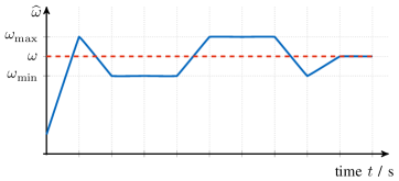
Usually, the grid frequency should not exceed a certain interval. This physically motivated limitation can be exploited for the frequency estimation. The principle idea of the proposed sign-correct anti-windup strategy is illustrated in Fig. 7. More precisely, the adaption of the estimated angular frequency shall be stopped (i.e. ddtω^=0dd𝑡^𝜔0\tfrac{\textrm{d}}{\textrm{d}t}\widehat{\omega}=0), when

  • the estimated angular frequency ω^^𝜔\widehat{\omega} leaves the admissible interval, i.e. ω^(ωmin,ωmax)^𝜔subscript𝜔subscript𝜔\widehat{\omega}\not\in(\omega_{\min},\,\omega_{\max}) with lower and upper limit 0<ωmin<ωmax0subscript𝜔subscript𝜔0<\omega_{\min}<\omega_{\max}, respectively (see Fig. 7); and

  • the right hand side of the adaption law (22) has wrong sign (otherwise the estimation gets stuck at one of the limits).

Refer to caption
Figure 7: Illustration of the principle idea of the proposed sign-correct anti-windup strategy.

This yields to the following sign-correct anti-windup decision function

faw(ω^,δ):={0, for (ω^ωmaxδddtω^0)(ω^ωminδddtω^0)1, elseassignsubscript𝑓aw^𝜔𝛿cases0 for ^𝜔subscript𝜔𝛿proportional-todd𝑡^𝜔0^𝜔subscript𝜔𝛿proportional-todd𝑡^𝜔0otherwise1 elseotherwisef_{\mathrm{aw}}(\widehat{\omega},\delta):=\begin{cases}0,\quad\text{ for }\;\big{(}\widehat{\omega}\geq\omega_{\max}\wedge\delta\propto\tfrac{\textrm{d}}{\textrm{d}t}\widehat{\omega}\geq 0\big{)}\vee\big{(}\widehat{\omega}\leq\omega_{\min}\wedge\delta\propto\tfrac{\textrm{d}}{\textrm{d}t}\widehat{\omega}\leq 0\big{)}\\ 1,\quad\text{ else}\end{cases} (24)

where δddtω^proportional-to𝛿dd𝑡^𝜔\delta\propto\tfrac{\textrm{d}}{\textrm{d}t}\widehat{\omega} is proportional to the time derivative of the estimated angular frequency as can be seen when decision function and frequency adaption law are combined as follows

ddtω^=faw(ω^,δ)Γω^ey𝝀𝒙^max(𝒙^12,ε)=:δ.dd𝑡^𝜔subscript𝑓aw^𝜔𝛿subscriptΓ^𝜔subscript𝑒𝑦superscript𝝀top^𝒙superscriptdelimited-∥∥subscript^𝒙12𝜀:absent𝛿\tfrac{\textrm{d}}{\textrm{d}t}\widehat{\omega}=f_{\mathrm{aw}}(\widehat{\omega},\delta)\underbrace{\tfrac{\Gamma\,\widehat{\omega}\,e_{y}\,\boldsymbol{\lambda}^{\top}\widehat{\boldsymbol{x}}}{\max\big{(}\left\lVert\widehat{\boldsymbol{x}}_{1}\right\rVert^{2},\varepsilon\big{)}}}_{=:\delta}. (25)

The consequences of this adaption law with sign-correct anti-windup are that the estimated angular frequency is positive and remains bounded for all time, i.e. ω^(t)[min(ω^0,ωmin),max(ω^0,ωmax)]^𝜔𝑡subscript^𝜔0subscript𝜔subscript^𝜔0subscript𝜔\widehat{\omega}(t)\in\big{[}\min(\widehat{\omega}_{0},\omega_{\min}),\,\max(\widehat{\omega}_{0},\omega_{\max})] for all t0𝑡0t\geq 0. Moreover, once within the admissible interval [ωmin,ωmax]subscript𝜔subscript𝜔[\omega_{\min},\omega_{\max}], the estimated angular frequency will remain inside this interval. Clearly, if the initial value ω^0subscript^𝜔0\widehat{\omega}_{0} of the frequency estimate starts outside of [ωmin,ωmax]subscript𝜔subscript𝜔[\omega_{\min},\omega_{\max}], it will approach the interval due to the sign-correct frequency adaption (as illustrated in Fig. 7 for ω^0<ωminsubscript^𝜔0subscript𝜔\widehat{\omega}_{0}<\omega_{\min}). Note that the proposed anti-windup strategy does not require tuning of an additional feedback gain as in [24]. Instability can not occur, since the proposed sign-correct anti-windup strategy is based on the simple idea of conditional integration [33, Section 10.4.1].

III-B3 Rate limitation

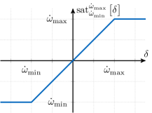
Recall that the overall observer (7) is nonlinear. Considering the estimated angular frequency as time-varying parameter, the observer becomes a time-varying linear system. If the time derivative ddtω^dd𝑡^𝜔\tfrac{\textrm{d}}{\textrm{d}t}\widehat{\omega} is limited (rate limitation), the observer can be considered as slowly time-varying system [34] (which simplifies stability analysis). For this rate limitation of the adaption law, the admissible rate of the estimated angular frequency must be bounded, i.e.  ddtω^[ω˙min,ω˙max]dd𝑡^𝜔subscript˙𝜔subscript˙𝜔\tfrac{\textrm{d}}{\textrm{d}t}\widehat{\omega}\in\big{[}\dot{\omega}_{\min},\dot{\omega}_{\max}\big{]} where ω˙min<0subscript˙𝜔0\dot{\omega}_{\min}<0 and ω˙max>0subscript˙𝜔0\dot{\omega}_{\max}>0 are desired lower and upper thresholds, respectively. The idea of the rate limitation is illustrated in the graph shown in Fig. 8.
Refer to caption
Figure 8: Illustration of the rate limitation of δddtω^proportional-to𝛿dd𝑡^𝜔\delta\propto\tfrac{\textrm{d}}{\textrm{d}t}\widehat{\omega}.

Usually, the rate limitation leads to a smoother adaption and ω˙min=ω˙maxsubscript˙𝜔subscript˙𝜔\dot{\omega}_{\min}=-\dot{\omega}_{\max} is a meaningful choice. Reasonable rate thresholds were found out to be 10100 Hz10times100hertzabsent10-$100\text{\,}\frac{\mathrm{Hz}}{}$ per 1 mstimes1millisecondabsent1\text{\,}\frac{\mathrm{ms}}{}. The rate limitation can be ensured by introducing an additional saturation function to the adaption law (25) leading to the generalized adaption law for the mFLL as shown next.

III-C Generalized adaption law

Finally, combining rate limitation, sign-correct anti-windup strategy and sFLL with gain normalization, the generalized adaption law of the mFLL with 𝝀𝝀\boldsymbol{\lambda} as in (23) can be introduced. It is given by

ddtω^=faw(ω^,δ)satω˙minω˙max[Γω^ey𝝀𝒙^max(𝒙^12,ε)=:δ]wherefaw(,)as in (24) andsatω˙minω˙max[δ]:={ω˙max,δ>ω˙maxδ,ω˙minδω˙maxω˙min,δ<ω˙min\boxed{\tfrac{\textrm{d}}{\textrm{d}t}\widehat{\omega}=f_{\mathrm{aw}}(\widehat{\omega},\delta)\cdot\operatorname{sat}_{\dot{\omega}_{\min}}^{\dot{\omega}_{\max}}\Big{[}\underbrace{\tfrac{\Gamma\,\widehat{\omega}\,e_{y}\,\boldsymbol{\lambda}^{\top}\widehat{\boldsymbol{x}}}{\max\big{(}\left\lVert\widehat{\boldsymbol{x}}_{1}\right\rVert^{2},\varepsilon\big{)}}}_{=:\delta}\Big{]}\;\text{where}\;f_{\mathrm{aw}}(\cdot,\cdot)\;\text{as in\leavevmode\nobreak\ \eqref{eq:sign-correct AW decision function} and}\;\operatorname{sat}_{\dot{\omega}_{\min}}^{\dot{\omega}_{\max}}\!\big{[}\delta\big{]}:=\begin{cases}\dot{\omega}_{\max}&,\delta>\dot{\omega}_{\max}\\ \delta&,\dot{\omega}_{\min}\leq\delta\leq\dot{\omega}_{\max}\\ \dot{\omega}_{\min}&,\delta<\dot{\omega}_{\min}\\ \end{cases}} (26)

which guarantees that (i) the derivative of the estimated angular frequency is bounded, i.e. ddtω^(t)[ω˙min,ω˙max]dd𝑡^𝜔𝑡subscript˙𝜔subscript˙𝜔\tfrac{\textrm{d}}{\textrm{d}t}\widehat{\omega}(t)\in\big{[}\dot{\omega}_{\min},\dot{\omega}_{\max}\big{]}, and (ii) the estimated angular frequency is positive and bounded from below and above, i.e. ω^(t)[min(ω^0,ωmin),max(ω^0,ωmax)]^𝜔𝑡subscript^𝜔0subscript𝜔subscript^𝜔0subscript𝜔\widehat{\omega}(t)\in\big{[}\min(\widehat{\omega}_{0},\omega_{\min}),\,\max(\widehat{\omega}_{0},\omega_{\max})] for all t0𝑡0t\geq 0.

IV Implementation and measurement results

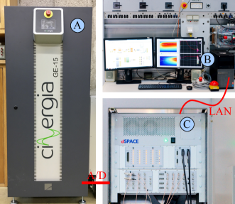
To validate the proposed algorithms, measurements at a laboratory setup are carried out. The laboratory setup is shown in Fig. 9.
Refer to caption
Figure 9: Laboratory setup: (A) Cinergia grid emulator, (B) Host-PC and (C) dSPACE real-time system .

For measurements, the voltage is produced by the grid emulator. These voltages are measured by a LEM DVL 500 voltage sensor, analogue-to-digital converted by the dSPACE A/D card DS2004 and internally filtered by a low pass filter with cut-off frequency ωlpf=5000radssubscript𝜔lpf5000radiansecond\omega_{\text{lpf}}=5000$\frac{\mathrm{rad}}{\mathrm{s}}$ to suppress high frequency noise. The implementation is done via Matlab/Simulink R2017a on the Host-PC. The executable observers are downloaded via LAN to the dSPACE Processor Board DS1007 and run in real time. The measurement data is captured and analyzed on the Host-PC after the experiment. The implementation data of the conducted measurements is listed in Tab. I.

Implementation
sampling time h=0,1 mstimes0.1millisecondabsenth=$0,1\text{\,}\frac{\mathrm{ms}}{}$
low-pass filter ωlpf=5103 radssubscript𝜔lpftimes5E3radiansecond\omega_{\text{lpf}}=$5\text{\cdot}{10}^{3}\text{\,}\frac{\mathrm{rad}}{\mathrm{s}}$ (for measurements)
parallelized mSOGIs
observer gains 𝒍𝒍\boldsymbol{l} as in (17) [νν:p1,2,ν=32±ȷν:absentfor-all𝜈subscript𝜈superscriptsubscript𝑝12𝜈plus-or-minus32italic-ȷ𝜈\Longrightarrow\;\forall\nu\in\mathbb{H}_{\nu}\colon\;p_{1,2,\nu}^{*}=-\tfrac{3}{2}\pm\jmath\nu]
mFLL Γ=60Γ60\Gamma=60, ε=0.1𝜀0.1\varepsilon=0.1
Anti-windup ωmin=39 radssubscript𝜔times39radiansecond\omega_{\min}=$39\text{\,}\frac{\mathrm{rad}}{\mathrm{s}}$, ωmax=61 radssubscript𝜔times61radiansecond\omega_{\max}=$61\text{\,}\frac{\mathrm{rad}}{\mathrm{s}}$
Rate limitation ω˙max=2π×10103 radssubscript˙𝜔2𝜋times10E3radiansecond\dot{\omega}_{\max}=2\pi\times$10\text{\cdot}{10}^{3}\text{\,}\frac{\mathrm{rad}}{\mathrm{s}}$, ω˙min=ω˙maxsubscript˙𝜔subscript˙𝜔\dot{\omega}_{\min}=-\dot{\omega}_{\max}
parallelized sSOGIs [7]
observer gains 𝒍=2𝒄𝒍2𝒄\boldsymbol{l}=\sqrt{2}\boldsymbol{c}
sFLL Γ=46Γ46\Gamma=46, ε=0.1𝜀0.1\varepsilon=0.1 (avoidance of division by zero added)
parallelized ANFs [4]
filter gains 𝒍=𝒄𝒍𝒄\boldsymbol{l}=\boldsymbol{c}
sFLL (without gain normalization) γ=0.5𝛾0.5\gamma=0.5
Scenario (S1) with constant fundamental frequency
initial values of observer (13) 𝒙^0=𝟎20subscript^𝒙0subscript020\widehat{\boldsymbol{x}}_{0}=\boldsymbol{0}_{20}
initial values of sFLL (21) and mFLL (26) ω^0=2π50 radssubscript^𝜔02𝜋times50radiansecond\widehat{\omega}_{0}=2\pi\cdot$50\text{\,}\frac{\mathrm{rad}}{\mathrm{s}}$ (and ω^(t)=ω(t)^𝜔𝑡𝜔𝑡\widehat{\omega}(t)=\omega(t) for all t0𝑡0t\geq 0)
Scenario (S2) with time-varying fundamental frequency
initial values of observer (13) 𝒙^0=𝟎20subscript^𝒙0subscript020\widehat{\boldsymbol{x}}_{0}=\boldsymbol{0}_{20}
initial values of sFLL (21) and mFLL (26) ω^0=200 radsω(0)=2π50 radssubscript^𝜔0times200radiansecond𝜔02𝜋times50radiansecond\widehat{\omega}_{0}=$200\text{\,}\frac{\mathrm{rad}}{\mathrm{s}}$\neq\omega(0)=2\pi\cdot$50\text{\,}\frac{\mathrm{rad}}{\mathrm{s}}$
Table I: Implementation and tuning data for simulations and measurements.

Three estimation methods are implemented and their estimation performances are compared for the following two scenarios:

  • (S1)

    Estimation of an input signal y𝑦y with constant fundamental angular frequency (i.e. ω^(t)=ω(t)=2π50 rads^𝜔𝑡𝜔𝑡2𝜋times50radiansecond\widehat{\omega}(t)=\omega(t)=2\pi$50\text{\,}\frac{\mathrm{rad}}{\mathrm{s}}$ for all t0𝑡0t\geq 0) and ten harmonics exhibiting amplitude jumps at t1=0,2 ssubscript𝑡1times0.2secondabsentt_{1}=$0,2\text{\,}\frac{\mathrm{s}}{}$, t2=0,4 ssubscript𝑡2times0.4secondabsentt_{2}=$0,4\text{\,}\frac{\mathrm{s}}{}$ and t3=0,6 ssubscript𝑡3times0.6secondabsentt_{3}=$0,6\text{\,}\frac{\mathrm{s}}{}$. The following three estimation methods are implemented and compared:

    • parallelized mSOGIs without FLL, i.e. observer (13) with 𝒍𝒍\boldsymbol{l} as in (17);

    • parallelized sSOGIs without FLL [7], i.e. observer (13) with 𝒍=2𝒄𝒍2𝒄\boldsymbol{l}=\sqrt{2}\boldsymbol{c} (and gν=0subscript𝑔𝜈0g_{\nu}=0 for all νn𝜈subscript𝑛\nu\in\mathbb{H}_{n}); and

    • parallelized Adaptive Notch Filters (ANFs) without FLL [4], i.e. observer (13) with 𝒍=𝒄𝒍𝒄\boldsymbol{l}=\boldsymbol{c}.

  • (S2)

    Estimation of an input signal y𝑦y with time-varying fundamental angular frequency ω()𝜔\omega(\cdot) (i.e. ω^0ω(0)subscript^𝜔0𝜔0\widehat{\omega}_{0}\neq\omega(0)) and ten harmonics exhibiting frequency jumps at t1=0,2 ssubscript𝑡1times0.2secondabsentt_{1}=$0,2\text{\,}\frac{\mathrm{s}}{}$ and t3=0,6 ssubscript𝑡3times0.6secondabsentt_{3}=$0,6\text{\,}\frac{\mathrm{s}}{}$ and amplitude jumps at t2=0,4 ssubscript𝑡2times0.4secondabsentt_{2}=$0,4\text{\,}\frac{\mathrm{s}}{}$ and t3=0,6 ssubscript𝑡3times0.6secondabsentt_{3}=$0,6\text{\,}\frac{\mathrm{s}}{}$. The following three estimation methods are implemented and compared:

    • parallelized mSOGIs with mFLL, i.e. (13) with 𝒍𝒍\boldsymbol{l} as in (17) and (26);

    • parallelized sSOGIs with sFLL [7], i.e. observer (13) with 𝒍=2𝒄𝒍2𝒄\boldsymbol{l}=\sqrt{2}\boldsymbol{c} (gν=0subscript𝑔𝜈0g_{\nu}=0 for all νn𝜈subscript𝑛\nu\in\mathbb{H}_{n}) and (21); and

    • parallelized ANFs with sFLL [4], i.e. observer (13) with 𝒍=𝒄𝒍𝒄\boldsymbol{l}=\boldsymbol{c} and sFLL (20) (without gain normalization444In [4], the gain is ’γ𝛾\gamma’ and set to 808080; the maximal amplitude is a1=1subscript𝑎11a_{1}=1. Because the Grid Emulator cannot produce such low voltages and the FLL is driven without a GN, the FLL gain for the ANFs is optimized here with respect to the used amplitudes.).

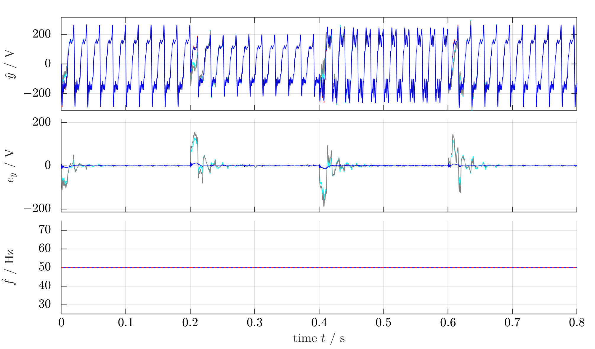
For both scenarios, the considered input signals y𝑦y have a significant harmonic distortion. The parameters of the individual harmonics (amplitudes aνsubscript𝑎𝜈a_{\nu} and frequencies f𝑓f) of the signal y𝑦y for Scenario (S1) and for Scenario (S2) are collected in Tab. II. Within the considered time interval [0,0,8 s]0times0.8secondabsent[0,\,$0,8\text{\,}\frac{\mathrm{s}}{}$], three jump-like changes in amplitudes and/or fundamental frequency occur at 0,2 stimes0.2secondabsent0,2\text{\,}\frac{\mathrm{s}}{}, 0,4 stimes0.4secondabsent0,4\text{\,}\frac{\mathrm{s}}{} and 0,6 stimes0.6secondabsent0,6\text{\,}\frac{\mathrm{s}}{}. Hence, the input signal and its harmonic content changes abruptly and requires the observers to “restart” their estimation process for each step-like change.

For a fair comparison, all three estimation methods are tuned in such a way that the best feasible estimation performance was achieved within their respective tuning and capability limits. The measurement results for Scenario (S1) are shown in the Figures 10, 11 and 12. The results for Scenario (S2) are depicted in Figures 13, 14 and 15. These results will be discussed in more detail in the next subsections.

[Uncaptioned image]
Table II: Data of considered input signal y𝑦y for both scenarios (S1) and (S2): Amplitudes and frequencies (f=ω2π𝑓𝜔2𝜋f=\tfrac{\omega}{2\pi}) of the ten harmonics.

IV-A Discussion of the measurement results obtained for Scenario (S1)

For Scenario (S1), the FLL were implemented but the adaption was turned off. Fundamental and estimated angular frequency are identical for this scenario. Therefore, the estimation performances purely according to the respective observer tunings can be compared. The harmonic content of the input signal y𝑦y undergoes step-like changes at the time instants 0,2 stimes0.2secondabsent0,2\text{\,}\frac{\mathrm{s}}{}, 0,4 stimes0.4secondabsent0,4\text{\,}\frac{\mathrm{s}}{} and 0,6 stimes0.6secondabsent0,6\text{\,}\frac{\mathrm{s}}{}, respectively (see Tab. II and Fig. 10).
Refer to caption
Figure 10: Measurement results for Scenario (S1): Comparison of the estimation performances of parallelized mSOGIs ( ), sSOGIs ( ) and ANFs ( ) without FLL. Signals shown from top to bottom are: Input signal y𝑦y ( ) & its estimate y^^𝑦\widehat{y}; estimation error ey=yy^subscript𝑒𝑦𝑦^𝑦e_{y}=y-\widehat{y}; frequency f=ω2π𝑓𝜔2𝜋f=\tfrac{\omega}{2\pi} ( ) & its estimate f^=ω^2π^𝑓^𝜔2𝜋\widehat{f}=\tfrac{\widehat{\omega}}{2\pi}.

Three measurement plots are presented in Figures 10, 11 and 12. The overall estimation performances of the parallelized mSOGIs ( ), sSOGIs ( ) and ANFs ( ) are depicted in Fig. 10: The first, second and third subplots show input signal y𝑦y ( ) & its estimates y^^𝑦\widehat{y}, the estimation errors ey=yy^subscript𝑒𝑦𝑦^𝑦e_{y}=y-\widehat{y} and fundamental frequency f𝑓f ( ) & its estimate f^=ω^2π^𝑓^𝜔2𝜋\widehat{f}=\tfrac{\widehat{\omega}}{2\pi}, respectively. All three observers are capable of estimating the input signal y𝑦y. All estimation errors ey0subscript𝑒𝑦0e_{y}\to 0 tend to zero after a certain time. The parallelized mSOGIs ( ) clearly outperform the other two estimation methods in estimation accuracy and estimation speed for all three step-like changes of the input signal y𝑦y at 0,2 stimes0.2secondabsent0,2\text{\,}\frac{\mathrm{s}}{}, 0,4 stimes0.4secondabsent0,4\text{\,}\frac{\mathrm{s}}{} and 0,6 stimes0.6secondabsent0,6\text{\,}\frac{\mathrm{s}}{}. Estimation is completed in less than 20 mstimes20millisecondabsent20\text{\,}\frac{\mathrm{ms}}{}. This is possibly due to the newly introduced gains gνsubscript𝑔𝜈g_{\nu} for all νn𝜈subscript𝑛\nu\in\mathbb{H}_{n} which give the necessary degrees of freedom in observer design (recall discussion in Sect. II-C).
Refer to caption Refer to caption
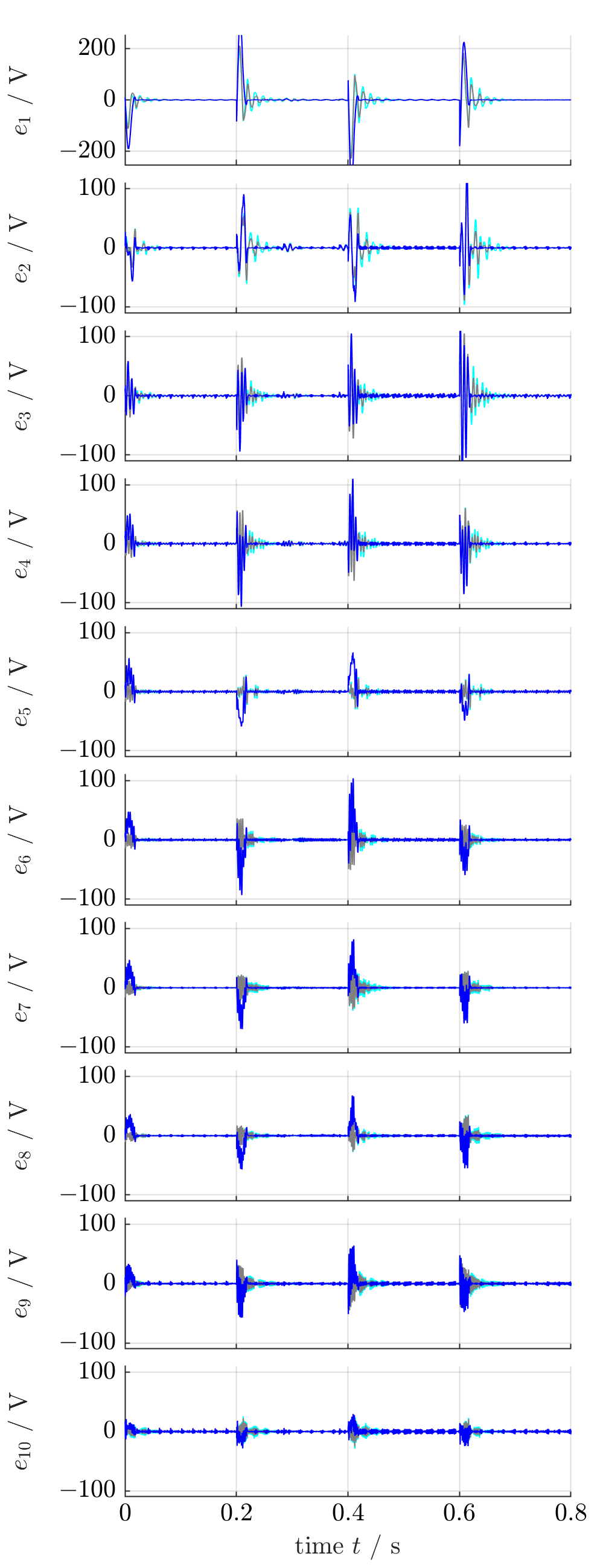
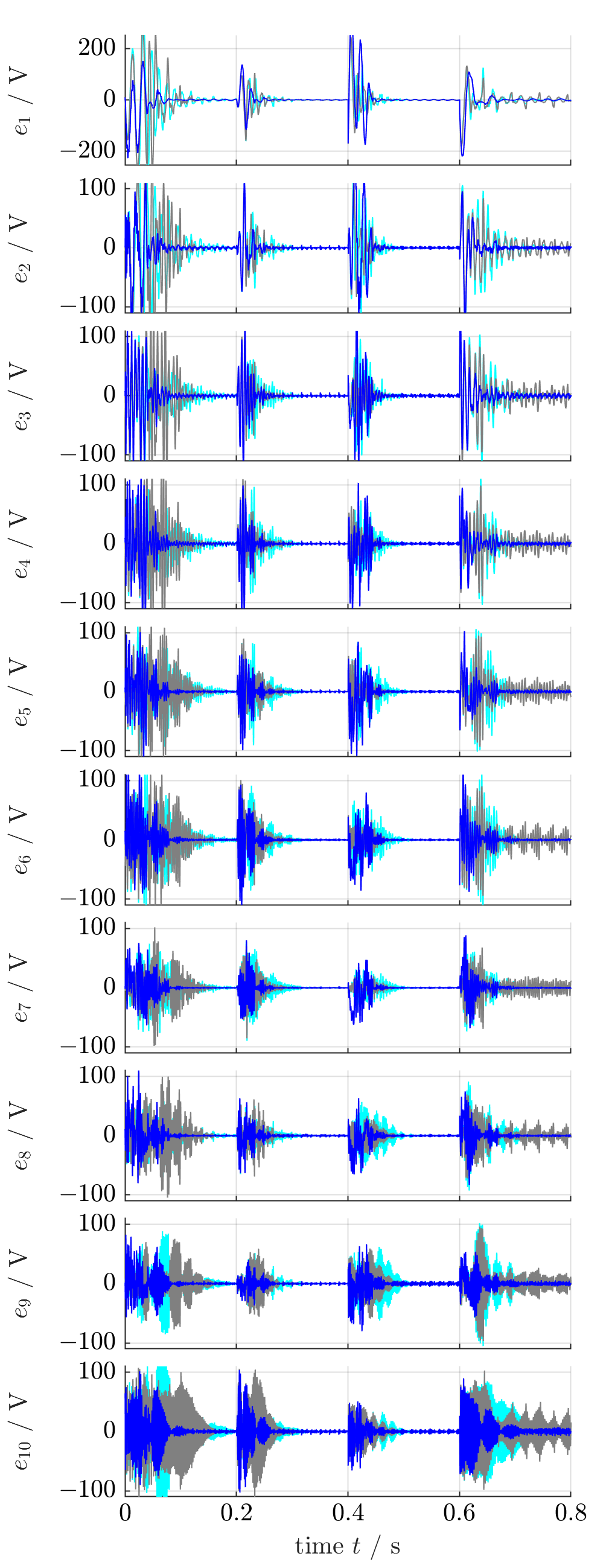
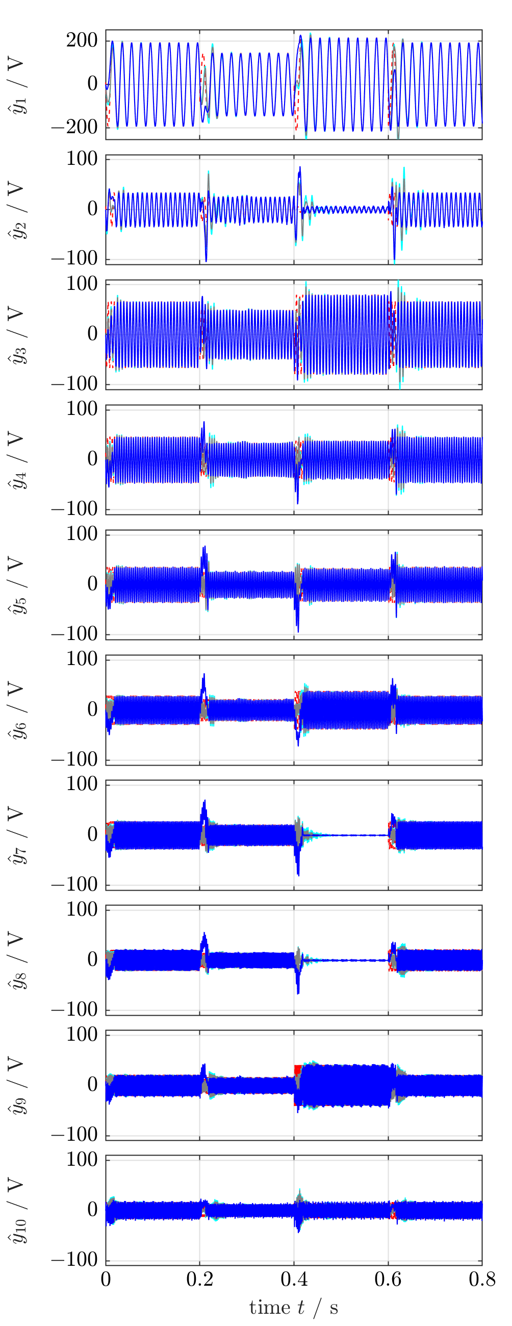
Figure 11: Measurement results for Scenario (S1): Comparison of the estimation performances of parallelized mSOGIs ( ), sSOGIs ( ) and ANFs ( ) without FLL. Signals shown from top to bottom are: Harmonic signals y1subscript𝑦1y_{1} to y10subscript𝑦10y_{10} ( ) & their estimates y^1subscript^𝑦1\widehat{y}_{1} to y^10subscript^𝑦10\widehat{y}_{10} (left) and harmonic estimation errors e1=y1y^1subscript𝑒1subscript𝑦1subscript^𝑦1e_{1}=y_{1}-\widehat{y}_{1} to e10=y10y^10subscript𝑒10subscript𝑦10subscript^𝑦10e_{10}=y_{10}-\widehat{y}_{10} (right).

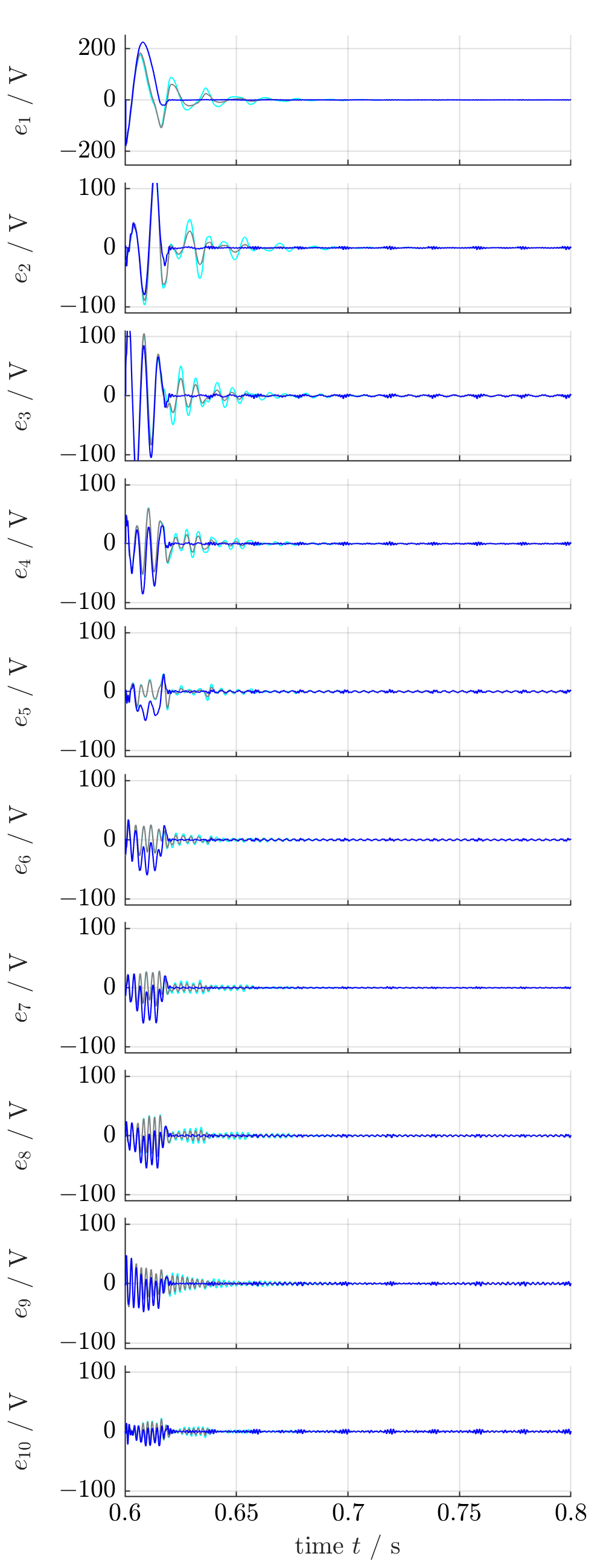
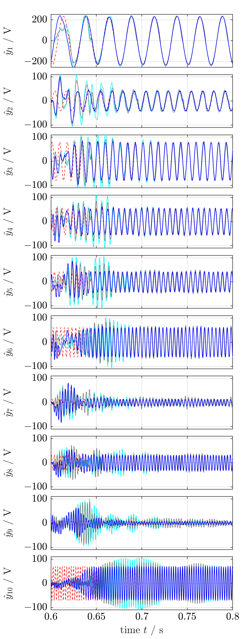
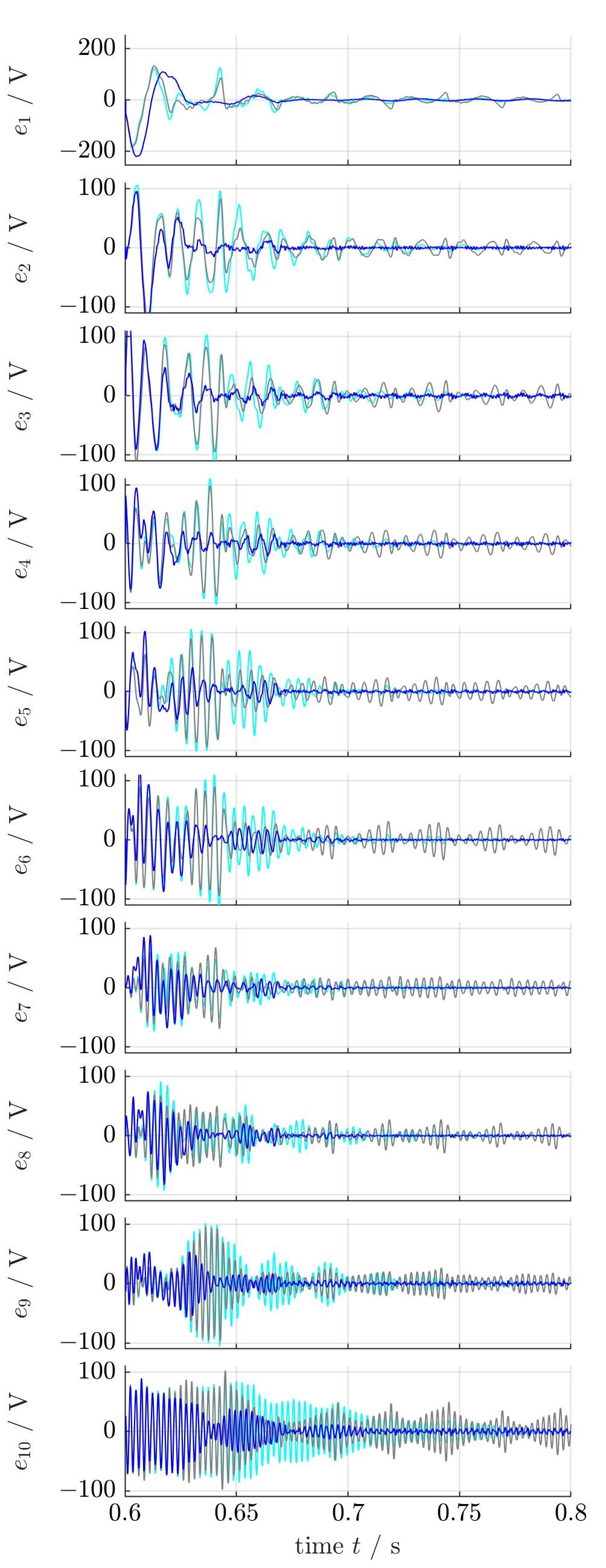
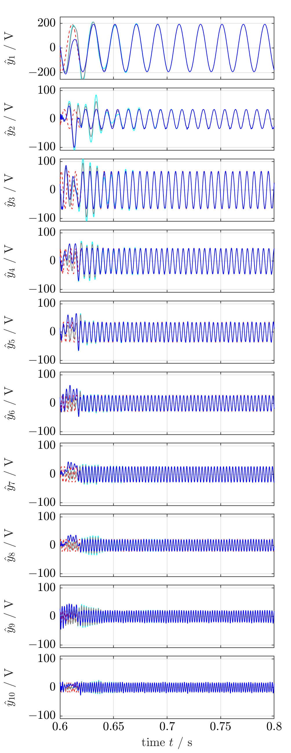
In Figures 11 and 12, the estimation performances for the ten individual harmonics are illustrated for the complete time interval [0,0,8 s]0times0.8secondabsent[0,\,$0,8\text{\,}\frac{\mathrm{s}}{}$] of Scenario (S1) (see Fig. 11) and for the shorter interval [0,6 s,0,8 s]times0.6secondabsenttimes0.8secondabsent[$0,6\text{\,}\frac{\mathrm{s}}{}$,\,$0,8\text{\,}\frac{\mathrm{s}}{}$] (see Zoom in Fig. 12), respectively. In both figures, on the left hand side, the harmonics y1subscript𝑦1y_{1} to y10subscript𝑦10y_{10} ( ) and theirs estimates y^1subscript^𝑦1\widehat{y}_{1} to y^10subscript^𝑦10\widehat{y}_{10} are shown; whereas on the right hand side, the estimation errors e1:=y1y^1assignsubscript𝑒1subscript𝑦1subscript^𝑦1e_{1}:=y_{1}-\widehat{y}_{1} to e10:=y10y^10assignsubscript𝑒10subscript𝑦10subscript^𝑦10e_{10}:=y_{10}-\widehat{y}_{10} are depicted. Again, all three estimation methods are capable of tracking the respective harmonic components after a certain time: Amplitudes and phases are estimated correctly with asymptotically vanishing estimation errors. But also for the individual harmonic estimation, the parallelized mSOGIs ( ) achieve a much faster estimation performance than the parallelized sSOGIs ( ) and the ANFs ( ). In particular for the lower harmonics (such as ν1=1subscript𝜈11\nu_{1}=1, ν2=2subscript𝜈22\nu_{2}=2, ν3=3subscript𝜈33\nu_{3}=3 and ν4=4subscript𝜈44\nu_{4}=4), the estimation is three to four times faster than that of the other two methods.
Refer to caption Refer to caption
Figure 12: Measurement results for Scenario (S1) – Zoom of time interval [0.6s,0.8s]0.6secondabsent0.8secondabsent[0.6$\frac{\mathrm{s}}{}$,0.8$\frac{\mathrm{s}}{}$]: Comparison of the estimation performances of parallelized mSOGIs ( ), sSOGIs ( ) and ANFs ( ) without FLL. Signals shown from top to bottom are: Harmonic signals y1subscript𝑦1y_{1} to y10subscript𝑦10y_{10} ( ) & their estimates y^1subscript^𝑦1\widehat{y}_{1} to y^10subscript^𝑦10\widehat{y}_{10} (left) and harmonic estimation errors e1=y1y^1subscript𝑒1subscript𝑦1subscript^𝑦1e_{1}=y_{1}-\widehat{y}_{1} to e10=y10y^10subscript𝑒10subscript𝑦10subscript^𝑦10e_{10}=y_{10}-\widehat{y}_{10} (right).

IV-B Discussion of the measurement results obtained for Scenario (S2)

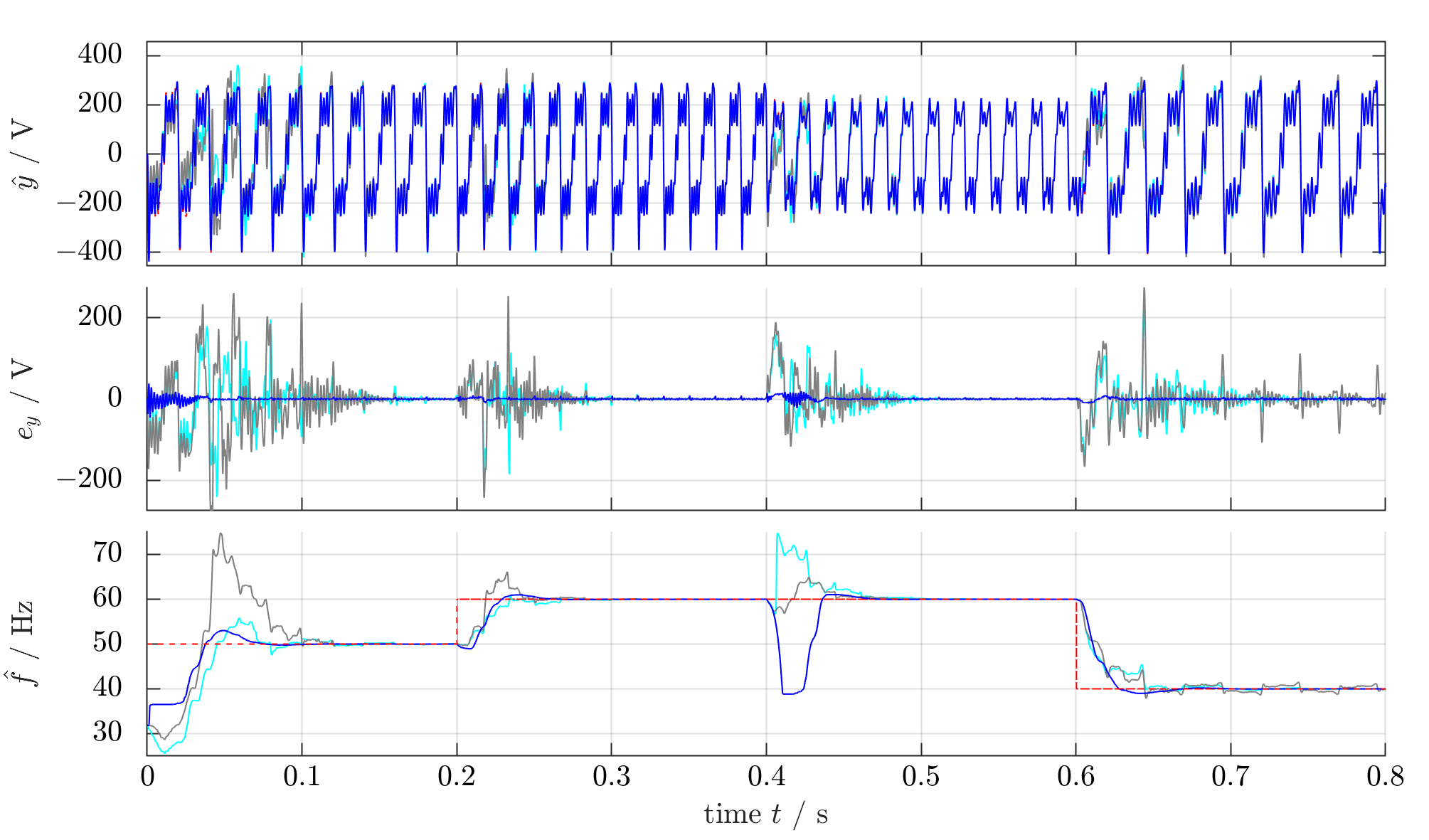
Scenario (S2) is more challenging. Now, amplitudes and frequency of the input signal y𝑦y are time-varying. At time instants 0,2 stimes0.2secondabsent0,2\text{\,}\frac{\mathrm{s}}{} and 0,6 stimes0.6secondabsent0,6\text{\,}\frac{\mathrm{s}}{}, the fundamental frequency jumps from 50 Hztimes50hertzabsent50\text{\,}\frac{\mathrm{Hz}}{} to 60 Hztimes60hertzabsent60\text{\,}\frac{\mathrm{Hz}}{} and from 60 Hztimes60hertzabsent60\text{\,}\frac{\mathrm{Hz}}{} to 40 Hztimes40hertzabsent40\text{\,}\frac{\mathrm{Hz}}{}, respectively; whereas amplitudes and phases of the harmonic components change abruptly at 0,4 stimes0.4secondabsent0,4\text{\,}\frac{\mathrm{s}}{} and 0,6 stimes0.6secondabsent0,6\text{\,}\frac{\mathrm{s}}{}, respectively (see Tab. II and Fig. 10). The measurement results for Scenario (S2) are plotted in Figures 10, 11 and 12. These figures show the identical quantities as those shown for Scenario (S1).
Refer to caption
Figure 13: Measurement results for Scenario (S2)Measurement results for Scenario (S1): Comparison of the estimation performances of parallelized mSOGIs ( ), sSOGIs ( ) and ANFs ( ) with FLL. Signals shown from top to bottom are: Input signal y𝑦y ( ) & its estimate y^^𝑦\widehat{y}; estimation error ey=yy^subscript𝑒𝑦𝑦^𝑦e_{y}=y-\widehat{y}; frequency f=ω2π𝑓𝜔2𝜋f=\tfrac{\omega}{2\pi} ( ) & its estimate f^=ω^2π^𝑓^𝜔2𝜋\widehat{f}=\tfrac{\widehat{\omega}}{2\pi}.

In Fig. 10, estimated signals y^^𝑦\widehat{y}, estimation errors ey:=yy^assignsubscript𝑒𝑦𝑦^𝑦e_{y}:=y-\widehat{y} and estimated frequencies f^^𝑓\widehat{f} are shown for the parallelized mSOGIs ( ), sSOGIs ( ) and ANFs ( ), respectively. All three estimation methods are able to correctly estimate the fundamental frequency asymptotically. But, for the parallelized mSOGIs, estimation accuracy and estimation speed of the proposed mFLL are better and the estimation process is much smoother and exhibits less oscillations. Please note that the dip in the frequency estimation of the mFLL after 0,4 stimes0.4secondabsent0,4\text{\,}\frac{\mathrm{s}}{} does not endanger stability of the parallelized mSOGIs (which is due to anti-windup and rate limitation). The overall estimation accuracy of the mSOGIs is very convincing as can be seen in eysubscript𝑒𝑦e_{y}. The estimation error tends to zero within 2040 ms20times40millisecondabsent20-$40\text{\,}\frac{\mathrm{ms}}{}$ after all three input changes at 0,2 stimes0.2secondabsent0,2\text{\,}\frac{\mathrm{s}}{}, 0,4 stimes0.4secondabsent0,4\text{\,}\frac{\mathrm{s}}{} and 0,6 stimes0.6secondabsent0,6\text{\,}\frac{\mathrm{s}}{} and remains close to zero afterwards. In contrast to that, the overall estimation accuracy and estimation speed of sSOGIs ( ) and ANFs ( ) are rather bad and slow: Rapid changes in eysubscript𝑒𝑦e_{y} occur for more than 100 mstimes100millisecondabsent100\text{\,}\frac{\mathrm{ms}}{} after each change. Within the last interval [0,6 s,0,8 s]times0.6secondabsenttimes0.8secondabsent[$0,6\text{\,}\frac{\mathrm{s}}{}$,\,$0,8\text{\,}\frac{\mathrm{s}}{}$], the estimation error of both methods does not even tend to zero within 200 mstimes200millisecondabsent200\text{\,}\frac{\mathrm{ms}}{}.

Similar observations can be made by comparing the individual harmonic estimation performances of the three estimation methods as shown in Fig. 11 for the overall time interval [0 s,0,8 s]times0secondabsenttimes0.8secondabsent[$0\text{\,}\frac{\mathrm{s}}{}$,\,$0,8\text{\,}\frac{\mathrm{s}}{}$] of Scenario (S2) and in Fig. 12 for the zoomed time interval [0,6 s,0,8 s]times0.6secondabsenttimes0.8secondabsent[$0,6\text{\,}\frac{\mathrm{s}}{}$,\,$0,8\text{\,}\frac{\mathrm{s}}{}$]. Despite the rather bad input estimation performance of parallelized sSOGIs ( ) and ANFs ( ), their harmonics estimation accuracy is acceptable: All harmonic amplitudes and angles are estimated correctly after some time. However, also here the estimation speed of the parallelized mSOGIs ( ) is faster for all harmonic components (see e1subscript𝑒1e_{1} to e10subscript𝑒10e_{10} in Fig. 11). However, the difference in estimation speed is not as significant as it was for Scenario (S1), which shows that the FLL remains the weakest component of the grid estimation process and has to be improved further (future work).

The last measurement plots depicted in Fig. 15 show the zoomed version of the harmonics estimation during the shorter time interval [0,6 s,0,8 s]times0.6secondabsenttimes0.8secondabsent[$0,6\text{\,}\frac{\mathrm{s}}{}$,\,$0,8\text{\,}\frac{\mathrm{s}}{}$]. Solely, the estimation performance of the parallelized mSOGIs ( ) is still acceptable. The estimation accuracies of parallelized sSOGIs ( ) and ANFs ( ) exhibit significant oscillations and do not tend to zero (in particular for higher harmonics). Their estimation performances are clearly not acceptable anymore. In conclusion, the measurement results obtained for both scenarios have verified the improved performance of the proposed parallelized mSOGIs ( ) with mFLL compared to the slower and less accurate estimation performances of parallelized sSOGI ( ) and ANFs ( ), respectively.
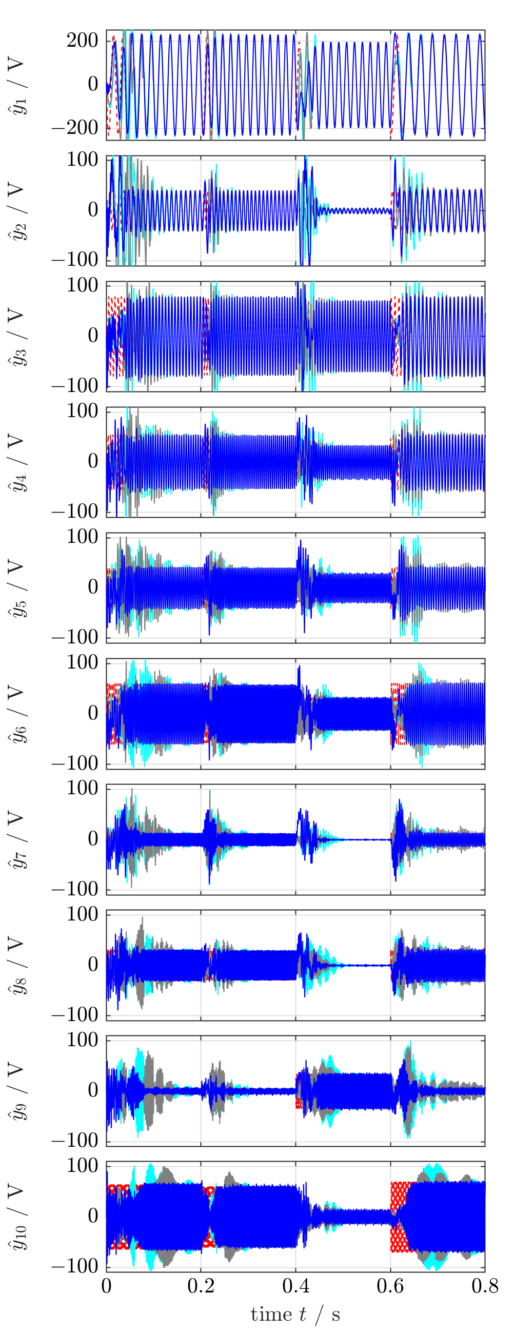
Refer to caption Refer to caption
Figure 14: Measurement results for Scenario (S2): Comparison of the estimation performances of parallelized mSOGIs ( ), sSOGIs ( ) and ANFs ( ) with FLL. Signals shown from top to bottom are: Harmonic signals y1subscript𝑦1y_{1} to y10subscript𝑦10y_{10} ( ) & their estimates y^1subscript^𝑦1\widehat{y}_{1} to y^10subscript^𝑦10\widehat{y}_{10} (left) and harmonic estimation errors e1=y1y^1subscript𝑒1subscript𝑦1subscript^𝑦1e_{1}=y_{1}-\widehat{y}_{1} to e10=y10y^10subscript𝑒10subscript𝑦10subscript^𝑦10e_{10}=y_{10}-\widehat{y}_{10} (right).
Refer to caption Refer to caption
Figure 15: Measurement results for Scenario (S2) – Zoom of time interval [0.6s,0.8s]0.6secondabsent0.8secondabsent[0.6$\frac{\mathrm{s}}{}$,0.8$\frac{\mathrm{s}}{}$]: Comparison of the estimation performances of parallelized mSOGIs ( ), sSOGIs ( ) and ANFs ( ) with FLL. Signals shown from top to bottom are: Harmonic signals y1subscript𝑦1y_{1} to y10subscript𝑦10y_{10} ( ) & their estimates y^1subscript^𝑦1\widehat{y}_{1} to y^10subscript^𝑦10\widehat{y}_{10} (left) and harmonic estimation errors e1=y1y^1subscript𝑒1subscript𝑦1subscript^𝑦1e_{1}=y_{1}-\widehat{y}_{1} to e10=y10y^10subscript𝑒10subscript𝑦10subscript^𝑦10e_{10}=y_{10}-\widehat{y}_{10} (right).

V Conclusion

A modified Second-Order Generalized Integrator (mSOGI) for the ν𝜈\nu-th harmonic component and a modified Frequency Locked Loop (mFLL) for the parallelized mSOGIs have been proposed. The number ν𝜈\nu can represent any positive not necessarily natural harmonic of an arbitrarily deteriorated input signal for which fundamental and higher harmonic components shall be estimated in real time. In contrast to the ν𝜈\nu-th standard SOGI (sSOGI) in literature, the ν𝜈\nu-th mSOGI allows (theoretically) for an arbitrarily fast estimation of the in-phase and quadrature signal of any specified harmonic component with prescribed settling time. This is possible due to an additionally introduced feedback gain in the mSOGI design. The proposed mFLL is equipped with sign-correct anti-windup strategy and rate limitation. These modifications enhance the frequency estimation in such a way that the frequency estimate remains positive and bounded and does not change too quickly (independently of mFLL tuning or operating point). Moreover, both enhancements overcome the stability problem of the estimator when a standard FLL (sFLL) is used. Measurement results illustrate and verify the improved estimation performance of the parallelized mSOGIs with and without mFLL in comparison to parallelized sSOGIs and ANFs with and without sFLL.

Future work will focus on (i) further improvements of the mFLL (acceleration of frequency estimation and global stability analysis), (ii) the extension of the presented results to three-phase signals (including DC offsets) and (iii) the real-time estimation of positive, negative and zero sequences of each harmonic component.

Appendix A Appendix

In the following appendices, observability and stability of the parallelized SOGIs, the pole placement algorithm and the generalization of the adaption law of the modified FLL for the parallelized mSOGIs are discussed in more detail.

A-A Recapitulation

Recall that, any exogenous sinusoidal signal of the form

y(t):=νnaν(t)cos(ϕν(t))=:yν(t) where n:={1,ν2,,νn},νiνj for all ij{1,,n}formulae-sequenceassign𝑦𝑡subscript𝜈subscript𝑛subscriptsubscript𝑎𝜈𝑡subscriptitalic-ϕ𝜈𝑡:absentsubscript𝑦𝜈𝑡 where formulae-sequenceassignsubscript𝑛1subscript𝜈2subscript𝜈𝑛formulae-sequencesubscript𝜈𝑖subscript𝜈𝑗 for all 𝑖𝑗1𝑛y(t):=\sum\limits_{\nu\in\mathbb{H}_{n}}\underbrace{a_{\nu}(t)\cos\big{(}\phi_{\nu}(t)\big{)}}_{=:y_{\nu}(t)}\quad\text{ where }\quad\mathbb{H}_{n}:=\{1,\nu_{2},\dots,\nu_{n}\},\quad\nu_{i}\neq\nu_{j}\quad\text{ for all }\quad i\neq j\in\left\{1,\ldots,n\right\}

can be reduplicated by the parallelization of n𝑛n sinusoidal internal models [33, Chapter 20]. The overall internal model dynamics are given by

ddt𝒙(t)=ω(t)𝑱𝒙(t),𝒙(0)=𝒙0𝟎2n2ny(t)=(1, 0, 1, 0,, 1, 0)=:𝒄2n𝒙(t)}\left.\begin{array}[]{rcl}\tfrac{\textrm{d}}{\textrm{d}t}\boldsymbol{x}(t)&=&\omega(t)\boldsymbol{J}\boldsymbol{x}(t),\qquad\qquad\qquad\qquad\boldsymbol{x}\left(0\right)=\boldsymbol{x}_{0}\neq\boldsymbol{0}_{2n}\in\mathbb{R}^{2n}\vspace*{1ex}\\ y(t)&=&\underbrace{(1,\,0,\,1,\,0,\,\cdots,\,1,\,0)}_{=:\,\boldsymbol{c}^{\top}\in\mathbb{R}^{2n}}\boldsymbol{x}(t)\end{array}\qquad\right\} (27)

where ω()𝒞pw(0;[ϵω,))𝜔superscript𝒞pwsuperscriptsubscriptabsent0subscriptitalic-ϵ𝜔\omega(\cdot)\in\mathcal{C}^{\mathrm{pw}}\cap\mathcal{L}^{\infty}(\mathbb{R}_{\geq 0};[\epsilon_{\omega},\infty)) (with ϵω>0subscriptitalic-ϵ𝜔0\epsilon_{\omega}>0) and

𝒙:=((x1α,x1β)=:𝒙1,,𝒙n),𝑱:=blockdiag(𝑱¯,ν2𝑱¯,,νn𝑱¯)2n×2n and 𝑱¯=[0110]=𝑱¯=𝑱¯1.\boldsymbol{x}:=\big{(}(\underbrace{x_{1}^{\alpha},\,x_{1}^{\beta})}_{=:\boldsymbol{x}_{1}^{\top}},\,\ldots,\,\boldsymbol{x}_{n}^{\top}\big{)}^{\top},\;\boldsymbol{J}:=\operatorname{blockdiag}\left(\overline{\boldsymbol{J}},\nu_{2}\overline{\boldsymbol{J}},\cdots,\nu_{n}\overline{\boldsymbol{J}}\right)\in\mathbb{R}^{2n\times 2n}\;\text{ and }\;\overline{\boldsymbol{J}}=\begin{bmatrix}0&-1\\ 1&0\end{bmatrix}=-\overline{\boldsymbol{J}}^{\top}=-\overline{\boldsymbol{J}}^{-1}. (28)

The initial values of the internal model in (27) allow to determine amplitude aνsubscript𝑎𝜈a_{\nu} and angle ϕνsubscriptitalic-ϕ𝜈\phi_{\nu} of the ν𝜈\nu-th harmonic component.

The overall observer (estimator) consists of the parallelized mSOGIs, i.e. the parallelized internal model (27) with feedback of the input signal y()𝑦y(\cdot) and using the estimated angular frequency ω^()^𝜔\widehat{\omega}(\cdot) instead of ω()𝜔\omega(\cdot). Its dynamics are given by

ddt𝒙^(t)=ω^(t)[𝑱𝒍𝒄=:𝑨]𝒙^(t)+ω^(t)𝒍y(t),𝒙^(t)=𝒙^02ny^(t)=𝒄𝒙^(t),}casesdd𝑡^𝒙𝑡^𝜔𝑡delimited-[]superscript𝑱𝒍superscript𝒄top:absent𝑨^𝒙𝑡^𝜔𝑡𝒍𝑦𝑡^𝒙𝑡subscript^𝒙0superscript2𝑛^𝑦𝑡superscript𝒄top^𝒙𝑡\left.\begin{array}[]{rcl}\tfrac{\textrm{d}}{\textrm{d}t}\widehat{\boldsymbol{x}}(t)&=&\widehat{\omega}(t)\big{[}\overbrace{\boldsymbol{J}-\boldsymbol{l}\boldsymbol{c}^{\top}}^{=:\boldsymbol{A}}\big{]}\widehat{\boldsymbol{x}}(t)+\widehat{\omega}(t)\,\boldsymbol{l}\,y(t),\qquad\qquad\widehat{\boldsymbol{x}}(t)=\widehat{\boldsymbol{x}}_{0}\in\mathbb{R}^{2n}\vspace*{2ex}\\ \widehat{y}(t)&=&\boldsymbol{c}^{\top}\widehat{\boldsymbol{x}}(t),\end{array}\right\} (29)

with observer state vector 𝒙^:=(𝒙^1,𝒙^ν2,,𝒙^νn)2nassign^𝒙superscriptsuperscriptsubscript^𝒙1topsuperscriptsubscript^𝒙subscript𝜈2topsuperscriptsubscript^𝒙subscript𝜈𝑛toptopsuperscript2𝑛\widehat{\boldsymbol{x}}:=\big{(}\widehat{\boldsymbol{x}}_{1}^{\top},\widehat{\boldsymbol{x}}_{\nu_{2}}^{\top},\cdots,\widehat{\boldsymbol{x}}_{\nu_{n}}^{\top}\big{)}^{\top}\in\mathbb{R}^{2n} and observer gain vector 𝒍:=(𝒍1,𝒍ν2,,𝒍νn)2n.assign𝒍superscriptsuperscriptsubscript𝒍1topsuperscriptsubscript𝒍subscript𝜈2topsuperscriptsubscript𝒍subscript𝜈𝑛toptopsuperscript2𝑛\boldsymbol{l}:=\big{(}\boldsymbol{l}_{1}^{\top},\boldsymbol{l}_{\nu_{2}}^{\top},\cdots,\boldsymbol{l}_{\nu_{n}}^{\top}\big{)}^{\top}\in\mathbb{R}^{2n}.

A-B Observability of the parallelized internal models (27) (for constant ω^^𝜔\widehat{\omega})

The grid state estimation algorithm is based on the idea of observability. The input signal can be considered to be generated by a parallelization of internal models which are individually capable of reduplicating a sinusoidal signal each (representing one harmonic component each). Hence, if this system is observable, an observer can be designed for grid state estimation.

Proposition A.1 (Observability of the linear generating system).

For constant ω>0𝜔0\omega>0 and differing harmonics, i.e. νiνjsubscript𝜈𝑖subscript𝜈𝑗\nu_{i}\neq\nu_{j} for all ij{1,n}𝑖𝑗1𝑛i\neq j\in\{1,\dots n\}, generating system (27) is completely state observable.

Proof.

Note that the following two identities hold

k:𝑱k=blockdiag(𝑱¯k,ν2k𝑱¯k,,νnk𝑱¯k)2n×2nand𝑱¯k=𝑱¯k22×2,\forall k\in\mathbb{N}\colon\qquad\boldsymbol{J}^{k}=\operatorname{blockdiag}\left(\overline{\boldsymbol{J}}^{k},\nu_{2}^{k}\overline{\boldsymbol{J}}^{k},\cdots,\nu_{n}^{k}\overline{\boldsymbol{J}}^{k}\right)\in\mathbb{R}^{2n\times 2n}\quad\text{and}\quad\overline{\boldsymbol{J}}^{k}=-\overline{\boldsymbol{J}}^{k-2}\in\mathbb{R}^{2\times 2},

which imply

rank[𝒄𝒄𝑱𝒄𝑱2𝒄𝑱3𝒄𝑱2n2𝒄𝑱2n1]rankmatrixsuperscript𝒄topsuperscript𝒄top𝑱superscript𝒄topsuperscript𝑱2superscript𝒄topsuperscript𝑱3superscript𝒄topsuperscript𝑱2𝑛2superscript𝒄topsuperscript𝑱2𝑛1\displaystyle\operatorname{rank}{\scriptsize\begin{bmatrix}\boldsymbol{c}^{\top}\\ \boldsymbol{c}^{\top}\boldsymbol{J}\\ \boldsymbol{c}^{\top}\boldsymbol{J}^{2}\\ \boldsymbol{c}^{\top}\boldsymbol{J}^{3}\\ \vdots\\ \boldsymbol{c}^{\top}\boldsymbol{J}^{2n-2}\\ \boldsymbol{c}^{\top}\boldsymbol{J}^{2n-1}\end{bmatrix}} =\displaystyle= rank[101010010ν20νn10ν220νn20010ν230νn3(1)n10(1)n1ν22n20(1)n1νn2n200(1)n0(1)nν22n10(1)nνn2n1]=2n.rankmatrix101010010subscript𝜈20subscript𝜈𝑛10superscriptsubscript𝜈220superscriptsubscript𝜈𝑛20010superscriptsubscript𝜈230superscriptsubscript𝜈𝑛3missing-subexpressionmissing-subexpressionmissing-subexpressionmissing-subexpressionsuperscript1𝑛10superscript1𝑛1superscriptsubscript𝜈22𝑛20superscript1𝑛1superscriptsubscript𝜈𝑛2𝑛200superscript1𝑛0superscript1𝑛superscriptsubscript𝜈22𝑛10superscript1𝑛superscriptsubscript𝜈𝑛2𝑛12𝑛\displaystyle\operatorname{rank}{\scriptsize\begin{bmatrix}1&0&1&0&\cdots&1&0\\ 0&-1&0&-\nu_{2}&\cdots&0&-\nu_{n}\\ -1&0&-\nu_{2}^{2}&0&\cdots&-\nu_{n}^{2}&0\\ 0&1&0&\nu_{2}^{3}&\cdots&0&\nu_{n}^{3}\\ \vdots&&&\vdots&&&\vdots\\ (-1)^{n-1}&0&(-1)^{n-1}\nu_{2}^{2n-2}&0&\cdots&(-1)^{n-1}\nu_{n}^{2n-2}&0\\ 0&(-1)^{n}&0&(-1)^{n}\nu_{2}^{2n-1}&\cdots&0&(-1)^{n}\nu_{n}^{2n-1}\\ \end{bmatrix}}=2n. (30)

Hence, the pair (𝑱,𝒄)𝑱superscript𝒄top(\boldsymbol{J},\boldsymbol{c}^{\top}) is observable [35, Corollary 12.3.19]. ∎

A-C Bounded-input bounded-state/bounded-output stability of the nonlinear observer

As first step, it is shown that for any essentially bounded input signal y()𝑦y(\cdot) and any essentially bounded and strictly positive estimated angular frequency ω^()^𝜔\widehat{\omega}(\cdot) the parallelized mSOGIs are bounded-input bounded-state/bounded-output state stable. In other words, the estimated states 𝒙^()^𝒙\widehat{\boldsymbol{x}}(\cdot) and the estimated output y^()^𝑦\widehat{y}(\cdot) will not diverge.

Theorem A.2 (Bounded-input bounded-state/bounded-output stability of the dynamics of the parallelized SOGIs).

Consider an essentially bounded input signal y()(0;)𝑦superscriptsubscriptabsent0y(\cdot)\in\mathcal{L}^{\infty}(\mathbb{R}_{\geq 0};\mathbb{R}) and assume that (i) the estimated time-varying fundamental angular frequency is continuous, bounded and uniformly bounded away from zero, i.e. ω^()𝒞(0;>0)(0;>0)^𝜔𝒞subscriptabsent0subscriptabsent0superscriptsubscriptabsent0subscriptabsent0\widehat{\omega}(\cdot)\in\mathcal{C}(\mathbb{R}_{\geq 0};\mathbb{R}_{>0})\cap\mathcal{L}^{\infty}(\mathbb{R}_{\geq 0};\mathbb{R}_{>0}) with ω^(t)ϵω>0^𝜔𝑡subscriptitalic-ϵ𝜔0\widehat{\omega}(t)\geq\epsilon_{\omega}>0 for all t0𝑡0t\geq 0, and (ii) the matrix 𝐀=𝐉𝐥𝐜𝐀𝐉𝐥superscript𝐜top\boldsymbol{A}=\boldsymbol{J}-\boldsymbol{l}\boldsymbol{c}^{\top} in (29) is a Hurwitz matrix. Then, the time-varying system (29) is bounded-input bounded-state/bounded-output stable, i.e.

t0cx,cy>0:𝒙^(t)cx and |y^(t)|cy.\forall t\geq 0\;\exists\,c_{x},\,c_{y}>0\colon\qquad\left\lVert\widehat{\boldsymbol{x}}(t)\right\rVert\leq c_{x}\quad\text{ and }\quad|\widehat{y}(t)|\leq c_{y}.
Proof.

First note that, since 𝑨𝑨\boldsymbol{A} is Hurwitz, there exists 𝑷=𝑷>0𝑷superscript𝑷top0\boldsymbol{P}=\boldsymbol{P}^{\top}>0 such that, for any given 𝑸=𝑸>0𝑸superscript𝑸top0\boldsymbol{Q}=\boldsymbol{Q}^{\top}>0, the following identity holds [31, Corollary 3.3.47]

𝑨𝑷+𝑷𝑨=𝑸.superscript𝑨top𝑷𝑷𝑨𝑸\boldsymbol{A}^{\top}\boldsymbol{P}+\boldsymbol{P}\boldsymbol{A}=-\boldsymbol{Q}. (31)

Moreover, note that

a,bm>0:2ab=a2m+mb2(ammb)2a2m+mb2.\forall\,a,b\in\mathbb{R}\;\forall\,m>0\colon\qquad 2\,a\,b=\tfrac{a^{2}}{m}+mb^{2}-\big{(}\tfrac{a}{\sqrt{m}}-\sqrt{m}\,b\big{)}^{2}\leq\tfrac{a^{2}}{m}+mb^{2}. (32)

Next, introduce the non-negative Lyapunov-like function

V:2n0,𝒙^V(𝒙^):=𝒙^𝑷𝒙^:𝑉formulae-sequencesuperscript2𝑛subscriptabsent0maps-to^𝒙𝑉^𝒙assignsuperscript^𝒙top𝑷^𝒙V\colon\mathbb{R}^{2n}\to\mathbb{R}_{\geq 0},\qquad\widehat{\boldsymbol{x}}\mapsto V(\widehat{\boldsymbol{x}}):=\widehat{\boldsymbol{x}}^{\top}\boldsymbol{P}\widehat{\boldsymbol{x}}

and denote minimal and maximal eigenvalue of 𝑷𝑷\boldsymbol{P} by λmin(𝑷)subscript𝜆𝑷\lambda_{\min}(\boldsymbol{P}) and λmax(𝑷)subscript𝜆𝑷\lambda_{\max}(\boldsymbol{P}), respectively. Then, clearly, the following holds

𝒙^2n:λmin(𝑷)𝒙^2V(𝒙^)λmax(𝑷)𝒙^2𝒙^21λmax(𝑷)V(𝒙^).\forall\,\widehat{\boldsymbol{x}}\in\mathbb{R}^{2n}\colon\qquad\lambda_{\min}(\boldsymbol{P})\left\lVert\widehat{\boldsymbol{x}}\right\rVert^{2}\leq V(\widehat{\boldsymbol{x}})\leq\lambda_{\max}(\boldsymbol{P})\left\lVert\widehat{\boldsymbol{x}}\right\rVert^{2}\quad\Longrightarrow\quad-\left\lVert\widehat{\boldsymbol{x}}\right\rVert^{2}\leq-\tfrac{1}{\lambda_{\max}(\boldsymbol{P})}V(\widehat{\boldsymbol{x}}). (33)

The right-hand side of (29) is locally Lipschitz continuous with bounded Lipschitz constant and bounded exogenous perturbation. Hence, the solution of (29) exists globally on 0subscriptabsent0\mathbb{R}_{\geq 0} [31, Theorem 2.2.14 & Proposition 2.2.19] (but still might diverge as t𝑡t\to\infty). The time derivative of V()𝑉V(\cdot) along the solution of (29) is, for all t0𝑡0t\geq 0, given and upper bounded by

ddtV(𝒙^(t))dd𝑡𝑉^𝒙𝑡\displaystyle\tfrac{\textrm{d}}{\textrm{d}t}V\big{(}\widehat{\boldsymbol{x}}(t)\big{)} =\displaystyle= ddt𝒙^(t)𝑷𝒙^(t)+𝒙^(t)𝑷ddt𝒙^(t)dd𝑡^𝒙superscript𝑡top𝑷^𝒙𝑡^𝒙superscript𝑡top𝑷dd𝑡^𝒙𝑡\displaystyle\tfrac{\textrm{d}}{\textrm{d}t}\widehat{\boldsymbol{x}}(t)^{\top}\boldsymbol{P}\widehat{\boldsymbol{x}}(t)+\widehat{\boldsymbol{x}}(t)^{\top}\boldsymbol{P}\tfrac{\textrm{d}}{\textrm{d}t}\widehat{\boldsymbol{x}}(t)
=(29)superscriptitalic-(29italic-)\displaystyle\stackrel{{\scriptstyle\eqref{eq:observer_sogi - appendix}}}{{=}} ω^(t)[𝒙^(t)(𝑨𝑷+𝑷𝑨)𝒙^(t)+y(t)𝒍𝑷𝒙^(t)+𝒙^(t)𝑷𝒍y(t)]^𝜔𝑡delimited-[]^𝒙superscript𝑡topsuperscript𝑨top𝑷𝑷𝑨^𝒙𝑡𝑦𝑡superscript𝒍top𝑷^𝒙𝑡^𝒙superscript𝑡top𝑷𝒍𝑦𝑡\displaystyle\widehat{\omega}(t)\Big{[}\widehat{\boldsymbol{x}}(t)^{\top}\big{(}\boldsymbol{A}^{\top}\boldsymbol{P}+\boldsymbol{P}\boldsymbol{A}\big{)}\widehat{\boldsymbol{x}}(t)+y(t)\boldsymbol{l}^{\top}\boldsymbol{P}\widehat{\boldsymbol{x}}(t)+\widehat{\boldsymbol{x}}(t)^{\top}\boldsymbol{P}\boldsymbol{l}y(t)\Big{]}
=\displaystyle= ω^(t)[𝒙^(t)(𝑨𝑷+𝑷𝑨)𝒙^(t)+2𝒙^(t)𝑷𝒍y(t)]^𝜔𝑡delimited-[]^𝒙superscript𝑡topsuperscript𝑨top𝑷𝑷𝑨^𝒙𝑡2^𝒙superscript𝑡top𝑷𝒍𝑦𝑡\displaystyle\widehat{\omega}(t)\Big{[}\widehat{\boldsymbol{x}}(t)^{\top}\big{(}\boldsymbol{A}^{\top}\boldsymbol{P}+\boldsymbol{P}\boldsymbol{A}\big{)}\widehat{\boldsymbol{x}}(t)+2\widehat{\boldsymbol{x}}(t)^{\top}\boldsymbol{P}\boldsymbol{l}y(t)\Big{]}
=(31)superscriptitalic-(31italic-)\displaystyle\stackrel{{\scriptstyle\eqref{eq:Lyapunov identity}}}{{=}} ω^(t)[𝒙^(t)𝑸𝒙^(t)+2𝒙^(t)𝑷𝒍y(t)]^𝜔𝑡delimited-[]^𝒙superscript𝑡top𝑸^𝒙𝑡2^𝒙superscript𝑡top𝑷𝒍𝑦𝑡\displaystyle\widehat{\omega}(t)\Big{[}-\widehat{\boldsymbol{x}}(t)^{\top}\boldsymbol{Q}\widehat{\boldsymbol{x}}(t)+2\widehat{\boldsymbol{x}}(t)^{\top}\boldsymbol{P}\boldsymbol{l}y(t)\Big{]}
(33)superscriptitalic-(33italic-)\displaystyle\stackrel{{\scriptstyle\eqref{eq:Inequalities for Lyapunov function}}}{{\leq}} ω^(t)[λmin(𝑸)𝒙^(t)2+2𝒙^(t)=:a𝑷𝒍y=:b]^𝜔𝑡delimited-[]subscript𝜆𝑸superscriptdelimited-∥∥^𝒙𝑡22subscriptdelimited-∥∥^𝒙𝑡:absent𝑎subscriptdelimited-∥∥𝑷delimited-∥∥𝒍subscriptnorm𝑦:absent𝑏\displaystyle\widehat{\omega}(t)\Big{[}-\lambda_{\min}(\boldsymbol{Q})\left\lVert\widehat{\boldsymbol{x}}(t)\right\rVert^{2}+2\underbrace{\left\lVert\widehat{\boldsymbol{x}}(t)\right\rVert}_{=:a}\underbrace{\left\lVert\boldsymbol{P}\right\rVert\left\lVert\boldsymbol{l}\right\rVert\|y\|_{\infty}}_{=:b}\Big{]}
(32)superscriptitalic-(32italic-)\displaystyle\stackrel{{\scriptstyle\eqref{eq:2ab<=...}}}{{\leq}} ω^(t)[(λmin(𝑸)1mm1 s.t. ()ϵm>0)𝒙^(t)2+m𝑷2𝒍2y2=:cm<]^𝜔𝑡delimited-[]subscriptsubscript𝜆𝑸1𝑚𝑚1 s.t. subscriptitalic-ϵ𝑚0superscriptdelimited-∥∥^𝒙𝑡2subscript𝑚superscriptdelimited-∥∥𝑷2superscriptdelimited-∥∥𝒍2superscriptsubscriptnorm𝑦2:absentsubscript𝑐𝑚absent\displaystyle\widehat{\omega}(t)\Big{[}-\big{(}\underbrace{\lambda_{\min}(\boldsymbol{Q})-\tfrac{1}{m}}_{\exists m\geq 1\text{ s.t. }(\cdot)\geq\epsilon_{m}>0}\big{)}\left\lVert\widehat{\boldsymbol{x}}(t)\right\rVert^{2}+\underbrace{m\left\lVert\boldsymbol{P}\right\rVert^{2}\left\lVert\boldsymbol{l}\right\rVert^{2}\|y\|_{\infty}^{2}}_{=:c_{m}<\infty}\Big{]}
(33)superscriptitalic-(33italic-)\displaystyle\stackrel{{\scriptstyle\eqref{eq:Inequalities for Lyapunov function}}}{{\leq}} [ϵmϵωλmax(𝑷)V(𝒙^(t))+cmω^]delimited-[]subscriptitalic-ϵ𝑚subscriptitalic-ϵ𝜔subscript𝜆𝑷𝑉^𝒙𝑡subscript𝑐𝑚subscriptnorm^𝜔\displaystyle\Big{[}-\tfrac{\epsilon_{m}\epsilon_{\omega}}{\lambda_{\max}(\boldsymbol{P})}V\big{(}\widehat{\boldsymbol{x}}(t)\big{)}+c_{m}\|\widehat{\omega}\|_{\infty}\Big{]}
V(𝒙^(t))absent𝑉^𝒙𝑡\displaystyle\Longrightarrow V\big{(}\widehat{\boldsymbol{x}}(t)\big{)} \displaystyle\leq V(𝒙^(0))+cmω^λmax(𝑷)ϵmϵω,𝑉^𝒙0subscript𝑐𝑚subscriptnorm^𝜔subscript𝜆𝑷subscriptitalic-ϵ𝑚subscriptitalic-ϵ𝜔\displaystyle V\big{(}\widehat{\boldsymbol{x}}(0)\big{)}+c_{m}\|\widehat{\omega}\|_{\infty}\tfrac{\lambda_{\max}(\boldsymbol{P})}{\epsilon_{m}\epsilon_{\omega}}, (34)

where, in the last step, the Bellman-Gronwall Lemma [36, p. 102f.] was used in its differential form (see Lemma 5.50 and Example 5.51 in [33]). Hence, in view of (33) and (34), and with 𝒄𝒄\boldsymbol{c} as in (27), one can conclude that

t0:𝒙^(t)(33),(34)1λmin(𝑷)(V(𝒙^(0))+cmω^λmax(𝑷)ϵmϵω)=:cx< and |y^(t)|(29)𝒄𝒙^(t)𝒄cx=:cy<,\forall\,t\geq 0\colon\left\lVert\widehat{\boldsymbol{x}}(t)\right\rVert\stackrel{{\scriptstyle\eqref{eq:Inequalities for Lyapunov function},\eqref{eq:Lyapunov analysis}}}{{\leq}}\sqrt{\tfrac{1}{\lambda_{\min}(\boldsymbol{P})}\Big{(}V\big{(}\widehat{\boldsymbol{x}}(0)\big{)}+c_{m}\|\widehat{\omega}\|_{\infty}\tfrac{\lambda_{\max}(\boldsymbol{P})}{\epsilon_{m}\epsilon_{\omega}}\Big{)}}=:c_{x}<\infty\\ \text{ and }\qquad|\widehat{y}(t)|\stackrel{{\scriptstyle\eqref{eq:observer_sogi - appendix}}}{{\leq}}\left\lVert\boldsymbol{c}\right\rVert\left\lVert\widehat{\boldsymbol{x}}(t)\right\rVert\leq\left\lVert\boldsymbol{c}\right\rVert c_{x}=:c_{y}<\infty,

which completes the proof. ∎

A-D Boundedness and exponential decay of the signal estimation error

It is shown that, for piecewise continuous (sinusoidal) and bounded input signals y()𝒞pw(0;)(0;)𝑦superscript𝒞pwsubscriptabsent0superscriptsubscriptabsent0y(\cdot)\in\mathcal{C}^{\textrm{pw}}(\mathbb{R}_{\geq 0};\mathbb{R})\cap\mathcal{L}^{\infty}(\mathbb{R}_{\geq 0};\mathbb{R}), the estimation error of the parallelized mSOGIs (or sSOGIs) is bounded. Additionally, if the piecewise constant fundamental angular frequency ω()𝜔\omega(\cdot) is correctly estimated, the estimation error decays exponentially.

To present the result, an important observation must be introduced. Note that, for ω()𝒞pw(0;[ϵω,))𝜔superscript𝒞pwsuperscriptsubscriptabsent0subscriptitalic-ϵ𝜔\omega(\cdot)\in\mathcal{C}^{\textrm{pw}}\cap\mathcal{L}^{\infty}(\mathbb{R}_{\geq 0};[\epsilon_{\omega},\infty)), any piecewise continuous (sinusoidal-like) signal of the form y()=νnaνcos(ν0ω(τ)dτ+ϕ0,ν)𝑦subscript𝜈subscript𝑛subscript𝑎𝜈𝜈superscriptsubscript0𝜔𝜏d𝜏subscriptitalic-ϕ0𝜈y(\cdot)=\sum_{\nu\in\mathbb{H}_{n}}a_{\nu}\cos\big{(}\nu\int_{0}^{\cdot}\omega(\tau)\textrm{d}\tau+\phi_{0,\nu}\big{)} on any bounded interval 𝕀i:=[ti,ti+1)assignsubscript𝕀𝑖subscript𝑡𝑖subscript𝑡𝑖1\mathbb{I}_{i}:=[t_{i},t_{i+1}), i0𝑖subscript0i\in\mathbb{N}_{0} (such that 0=𝕀0𝕀1𝕀2subscriptabsent0subscript𝕀0subscript𝕀1subscript𝕀2\mathbb{R}_{\geq 0}=\mathbb{I}_{0}\cup\mathbb{I}_{1}\cup\mathbb{I}_{2}\cup\dots) can be generated by (the output of) a properly initialized internal model [37] of the following form

t𝕀i:ddt𝒙(t)=ω(t)𝑱𝒙(t),𝒙(ti)=𝒙i,02ny(t)=𝒄𝒙(t)}\left.\begin{array}[]{rcl}\forall\,t\in\mathbb{I}_{i}\colon\quad\tfrac{\textrm{d}}{\textrm{d}t}\boldsymbol{x}(t)&=&\omega(t)\,\boldsymbol{J}\boldsymbol{x}(t),\qquad\boldsymbol{x}(t_{i})=\boldsymbol{x}_{i,0}\in\mathbb{R}^{2n}\vspace*{1ex}\\ y(t)&=&\boldsymbol{c}^{\top}\boldsymbol{x}(t)\end{array}\qquad\right\} (35)

with 𝑱𝑱\boldsymbol{J} as in (28). ω()𝜔\omega(\cdot) can be considered as an external input to the internal model. Clearly, for any real (finite) initial value 𝒙i,02nsubscript𝒙𝑖0superscript2𝑛\boldsymbol{x}_{i,0}\in\mathbb{R}^{2n} for the i𝑖i-th time interval 𝕀isubscript𝕀𝑖\mathbb{I}_{i}, all states of the internal model (35) are essentially bounded, i.e. 𝒙()(0;2n)𝒙superscriptsubscriptabsent0superscript2𝑛\boldsymbol{x}(\cdot)\in\mathcal{L}^{\infty}(\mathbb{R}_{\geq 0};\mathbb{R}^{2n}). Note that ω()𝜔\omega(\cdot), ϕ0,νsubscriptitalic-ϕ0𝜈\phi_{0,\nu} and aνsubscript𝑎𝜈a_{\nu} for all νn𝜈subscript𝑛\nu\in\mathbb{H}_{n} might change for each interval 𝕀isubscript𝕀𝑖\mathbb{I}_{i}. Now, the result can be stated.

Theorem A.3 (Boundedness and exponential decay of the signal estimation error).

Let ϵω>0subscriptitalic-ϵ𝜔0\epsilon_{\omega}>0, n={ν1,ν2,,νn}subscript𝑛subscript𝜈1subscript𝜈2subscript𝜈𝑛\mathbb{H}_{n}=\{\nu_{1},\nu_{2},\dots,\nu_{n}\}, aν0subscript𝑎𝜈0a_{\nu}\geq 0, ϕ0,νsubscriptitalic-ϕ0𝜈\phi_{0,\nu} for all νn𝜈subscript𝑛\nu\in\mathbb{H}_{n} and ω^(),ω()𝒞pw(0;[ϵω,))^𝜔𝜔superscript𝒞pwsuperscriptsubscriptabsent0subscriptitalic-ϵ𝜔\widehat{\omega}(\cdot),\,\omega(\cdot)\in\mathcal{C}^{\textrm{pw}}\cap\mathcal{L}^{\infty}(\mathbb{R}_{\geq 0};[\epsilon_{\omega},\infty)). Consider any piecewise continuous and bounded input signals, i.e. y()=νnaνcos(ν0ω(τ)dτ+ϕ0,ν)𝒞pw(0;)𝑦subscript𝜈subscript𝑛subscript𝑎𝜈𝜈superscriptsubscript0𝜔𝜏d𝜏subscriptitalic-ϕ0𝜈superscript𝒞pwsuperscriptsubscriptabsent0y(\cdot)=\sum_{\nu\in\mathbb{H}_{n}}a_{\nu}\cos\big{(}\nu\int_{0}^{\cdot}\omega(\tau)\textrm{d}\tau+\phi_{0,\nu}\big{)}\in\mathcal{C}^{\textrm{pw}}\cap\mathcal{L}^{\infty}(\mathbb{R}_{\geq 0};\mathbb{R}) on any bounded interval 𝕀i:=[ti,ti+1)assignsubscript𝕀𝑖subscript𝑡𝑖subscript𝑡𝑖1\mathbb{I}_{i}:=[t_{i},t_{i+1}), i0𝑖subscript0i\in\mathbb{N}_{0} (such that 0=𝕀0𝕀1𝕀2subscriptabsent0subscript𝕀0subscript𝕀1subscript𝕀2italic-…\mathbb{R}_{\geq 0}=\mathbb{I}_{0}\cup\mathbb{I}_{1}\cup\mathbb{I}_{2}\cup\dots), generated by the internal model (35) and assume that y()𝑦y(\cdot) is fed to the parallelized SOGI system (29) with 𝐀:=𝐉𝐥𝐜assign𝐀𝐉𝐥superscript𝐜top\boldsymbol{A}:=\boldsymbol{J}-\boldsymbol{l}\boldsymbol{c}^{\top} being a Hurwitz matrix. Then, the estimation error, defined by

𝒆x(t):=𝒙(t)𝒙^(t)2nassignsubscript𝒆𝑥𝑡𝒙𝑡^𝒙𝑡superscript2𝑛\boldsymbol{e}_{x}(t):=\boldsymbol{x}(t)-\widehat{\boldsymbol{x}}(t)\in\mathbb{R}^{2n} (36)

with 𝐱(t)𝐱𝑡\boldsymbol{x}(t) as in (35) and 𝐱^(t)^𝐱𝑡\widehat{\boldsymbol{x}}(t) as in (29), is bounded, i.e. there exists ce>0subscript𝑐𝑒0c_{e}>0 such that 𝐞x(t)cedelimited-∥∥subscript𝐞𝑥𝑡subscript𝑐𝑒\left\lVert\boldsymbol{e}_{x}(t)\right\rVert\leq c_{e} for all t0𝑡0t\geq 0. Moreover, if, for some i0𝑖subscript0i\in\mathbb{N}_{0}, ω(t)=ω^(t)𝜔𝑡^𝜔𝑡\omega(t)=\widehat{\omega}(t) for all t𝕀ss𝕀i𝑡subscript𝕀sssubscript𝕀𝑖t\in\mathbb{I}_{\textrm{ss}}\subseteq\mathbb{I}_{i}, then the norm of the estimation error is exponentially decaying, i.e. there exist constants cV,μV>0subscript𝑐𝑉subscript𝜇𝑉0c_{V},\,\mu_{V}>0 such that 𝐞x(t)cV𝐞x(ti)\eμV(tti)delimited-∥∥subscript𝐞𝑥𝑡subscript𝑐𝑉delimited-∥∥subscript𝐞𝑥subscript𝑡𝑖superscript\esubscript𝜇𝑉𝑡subscript𝑡𝑖\left\lVert\boldsymbol{e}_{x}(t)\right\rVert\leq c_{V}\,\left\lVert\boldsymbol{e}_{x}(t_{i})\right\rVert\e^{-\mu_{V}(t-t_{i})} for all t𝕀ss𝑡subscript𝕀sst\in\mathbb{I}_{\textrm{ss}}.

Proof.

Note that, for any interval 𝕀isubscript𝕀𝑖\mathbb{I}_{i}, combining (29) and (35) yields

t𝕀i:ddt(𝒙^(t)𝒙(t))4n=[ω^(t)𝑨ω^(t)𝒍𝒄𝑶2n×2nω(t)𝑱](𝒙^(t)𝒙(t)),(𝒙^(ti)𝒙(ti))=(𝒙^i,0𝒙i,0)4n.\forall\,t\in\mathbb{I}_{i}\colon\quad\tfrac{\textrm{d}}{\textrm{d}t}\underbrace{\begin{pmatrix}\widehat{\boldsymbol{x}}(t)\\ \boldsymbol{x}(t)\end{pmatrix}}_{\in\mathbb{R}^{4n}}=\begin{bmatrix}\widehat{\omega}(t)\boldsymbol{A}&\widehat{\omega}(t)\boldsymbol{l}\boldsymbol{c}^{\top}\\ \boldsymbol{O}_{2n\times 2n}&\omega(t)\boldsymbol{J}\end{bmatrix}\begin{pmatrix}\widehat{\boldsymbol{x}}(t)\\ \boldsymbol{x}(t)\end{pmatrix},\qquad\begin{pmatrix}\widehat{\boldsymbol{x}}(t_{i})\\ \boldsymbol{x}(t_{i})\end{pmatrix}=\begin{pmatrix}\widehat{\boldsymbol{x}}_{i,0}\\ \boldsymbol{x}_{i,0}\end{pmatrix}\in\mathbb{R}^{4n}. (37)

Next, introduce the angular frequency estimation error

t𝕀i:eω(t):=ω(t)ω^(t)ω(t)=eω(t)+ω^(t),\forall\,t\in\mathbb{I}_{i}\colon\quad e_{\omega}(t):=\omega(t)-\widehat{\omega}(t)\quad\Longleftrightarrow\quad\omega(t)=e_{\omega}(t)+\widehat{\omega}(t), (38)

and evaluate the time derivative of the estimation error vector as follows

t𝕀i:ddt(𝒙(t)𝒙^(t))=(36)𝒆x(t)\displaystyle\forall\,t\in\mathbb{I}_{i}\colon\quad\tfrac{\textrm{d}}{\textrm{d}t}\underbrace{\big{(}\boldsymbol{x}(t)-\widehat{\boldsymbol{x}}(t)\big{)}}_{\stackrel{{\scriptstyle\eqref{eq:estimation error vector}}}{{=}}\boldsymbol{e}_{x}(t)} =\displaystyle= [𝑰2n𝑰2n]ddt(𝒙^(t)𝒙(t))matrixsubscript𝑰2𝑛subscript𝑰2𝑛dd𝑡matrix^𝒙𝑡𝒙𝑡\displaystyle\begin{bmatrix}-\boldsymbol{I}_{2n}&\boldsymbol{I}_{2n}\\ \end{bmatrix}\tfrac{\textrm{d}}{\textrm{d}t}\begin{pmatrix}\widehat{\boldsymbol{x}}(t)\\ \boldsymbol{x}(t)\end{pmatrix} (39)
=(37)superscriptitalic-(37italic-)\displaystyle\stackrel{{\scriptstyle\eqref{eq:parallelized SOGIs and IM}}}{{=}} ω^(t)𝑨𝒙^(t)(ω^(t)𝒍𝒄ω(t)𝑱)𝒙(t)^𝜔𝑡𝑨^𝒙𝑡^𝜔𝑡𝒍superscript𝒄top𝜔𝑡𝑱𝒙𝑡\displaystyle-\widehat{\omega}(t)\boldsymbol{A}\widehat{\boldsymbol{x}}(t)-\Big{(}\widehat{\omega}(t)\boldsymbol{l}\boldsymbol{c}^{\top}-\omega(t)\boldsymbol{J}\Big{)}\boldsymbol{x}(t)
=(38)superscriptitalic-(38italic-)\displaystyle\stackrel{{\scriptstyle\eqref{eq:angular frequency error}}}{{=}} ω^(t)𝑨𝒙^(t)ω^(t)(𝒍𝒄𝑱)=(29)𝑨𝒙(t)+eω(t)𝑱𝒙(t)^𝜔𝑡𝑨^𝒙𝑡^𝜔𝑡subscript𝒍superscript𝒄top𝑱superscriptitalic-(29italic-)absent𝑨𝒙𝑡subscript𝑒𝜔𝑡𝑱𝒙𝑡\displaystyle-\widehat{\omega}(t)\boldsymbol{A}\widehat{\boldsymbol{x}}(t)-\widehat{\omega}(t)\underbrace{\big{(}\boldsymbol{l}\boldsymbol{c}^{\top}-\boldsymbol{J}\big{)}}_{\stackrel{{\scriptstyle\eqref{eq:observer_sogi - appendix}}}{{=}}-\boldsymbol{A}}\boldsymbol{x}(t)+e_{\omega}(t)\boldsymbol{J}\boldsymbol{x}(t)
=\displaystyle= ω^(t)𝑨𝒆x(t)+eω(t)𝑱𝒙(t).^𝜔𝑡𝑨subscript𝒆𝑥𝑡subscript𝑒𝜔𝑡𝑱𝒙𝑡\displaystyle\widehat{\omega}(t)\boldsymbol{A}\boldsymbol{e}_{x}(t)+e_{\omega}(t)\boldsymbol{J}\boldsymbol{x}(t).

Now, the time derivative of the Lyapunov-like function V(𝒆x())=𝒆x()𝑷𝒆x()𝑉subscript𝒆𝑥subscript𝒆𝑥superscripttop𝑷subscript𝒆𝑥V(\boldsymbol{e}_{x}(\cdot))=\boldsymbol{e}_{x}(\cdot)^{\top}\boldsymbol{P}\boldsymbol{e}_{x}(\cdot) (with 𝑷𝑷\boldsymbol{P} as introduced in (31)) is given for all t𝕀i=[ti,ti+1)𝑡subscript𝕀𝑖subscript𝑡𝑖subscript𝑡𝑖1t\in\mathbb{I}_{i}=[t_{i},\,t_{i+1}), along the solution of (39), as follows

ddtV(𝒆x(t))dd𝑡𝑉subscript𝒆𝑥𝑡\displaystyle\tfrac{\textrm{d}}{\textrm{d}t}V\big{(}\boldsymbol{e}_{x}(t)\big{)} =\displaystyle= ddt𝒆x(t)𝑷𝒆x(t)+𝒆x(t)𝑷ddt𝒆x(t)dd𝑡subscript𝒆𝑥superscript𝑡top𝑷subscript𝒆𝑥𝑡subscript𝒆𝑥superscript𝑡top𝑷dd𝑡subscript𝒆𝑥𝑡\displaystyle\tfrac{\textrm{d}}{\textrm{d}t}\boldsymbol{e}_{x}(t)^{\top}\boldsymbol{P}\boldsymbol{e}_{x}(t)+\boldsymbol{e}_{x}(t)^{\top}\boldsymbol{P}\tfrac{\textrm{d}}{\textrm{d}t}\boldsymbol{e}_{x}(t)
=(39)superscriptitalic-(39italic-)\displaystyle\stackrel{{\scriptstyle\eqref{eq:dynamics of estimation error}}}{{=}} ω^(t)𝒆x(t)(𝑨𝑷+𝑷𝑨)𝒆x(t)+eω(t)(𝒆x(t)𝑷𝑱𝒙(t)+𝒙(t)𝑱𝑷𝒆x(t))^𝜔𝑡subscript𝒆𝑥superscript𝑡topsuperscript𝑨top𝑷𝑷𝑨subscript𝒆𝑥𝑡subscript𝑒𝜔𝑡subscript𝒆𝑥superscript𝑡top𝑷𝑱𝒙𝑡𝒙superscript𝑡topsuperscript𝑱top𝑷subscript𝒆𝑥𝑡\displaystyle\widehat{\omega}(t)\boldsymbol{e}_{x}(t)^{\top}\big{(}\boldsymbol{A}^{\top}\boldsymbol{P}+\boldsymbol{P}\boldsymbol{A}\big{)}\boldsymbol{e}_{x}(t)+e_{\omega}(t)\big{(}\boldsymbol{e}_{x}(t)^{\top}\boldsymbol{P}\boldsymbol{J}\boldsymbol{x}(t)+\boldsymbol{x}(t)^{\top}\boldsymbol{J}^{\top}\boldsymbol{P}\boldsymbol{e}_{x}(t)\big{)}
=\displaystyle= ω^(t)𝒆x(t)(𝑨𝑷+𝑷𝑨)𝒆x(t)+2eω(t)𝒆x(t)𝑷𝑱𝒙(t)^𝜔𝑡subscript𝒆𝑥superscript𝑡topsuperscript𝑨top𝑷𝑷𝑨subscript𝒆𝑥𝑡2subscript𝑒𝜔𝑡subscript𝒆𝑥superscript𝑡top𝑷𝑱𝒙𝑡\displaystyle\widehat{\omega}(t)\boldsymbol{e}_{x}(t)^{\top}\big{(}\boldsymbol{A}^{\top}\boldsymbol{P}+\boldsymbol{P}\boldsymbol{A}\big{)}\boldsymbol{e}_{x}(t)+2e_{\omega}(t)\boldsymbol{e}_{x}(t)^{\top}\boldsymbol{P}\boldsymbol{J}\boldsymbol{x}(t)
=(31)superscriptitalic-(31italic-)\displaystyle\stackrel{{\scriptstyle\eqref{eq:Lyapunov identity}}}{{=}} ω^(t)𝒆x(t)𝑸𝒆x(t)+2eω(t)𝒆x(t)𝑷𝑱𝒙(t)^𝜔𝑡subscript𝒆𝑥superscript𝑡top𝑸subscript𝒆𝑥𝑡2subscript𝑒𝜔𝑡subscript𝒆𝑥superscript𝑡top𝑷𝑱𝒙𝑡\displaystyle-\widehat{\omega}(t)\boldsymbol{e}_{x}(t)^{\top}\boldsymbol{Q}\boldsymbol{e}_{x}(t)+2e_{\omega}(t)\boldsymbol{e}_{x}(t)^{\top}\boldsymbol{P}\boldsymbol{J}\boldsymbol{x}(t)
(33)superscriptitalic-(33italic-)\displaystyle\stackrel{{\scriptstyle\eqref{eq:Inequalities for Lyapunov function}}}{{\leq}} ω^(t)λmin(𝑸)𝒆x(t)2+2ω^(t)𝒆x(t)=:a|eω(t)|𝑷𝑱𝒙1ω^(t)=:b^𝜔𝑡subscript𝜆𝑸superscriptdelimited-∥∥subscript𝒆𝑥𝑡22subscript^𝜔𝑡delimited-∥∥subscript𝒆𝑥𝑡:absent𝑎subscriptsubscript𝑒𝜔𝑡delimited-∥∥𝑷delimited-∥∥𝑱subscriptnorm𝒙1^𝜔𝑡:absent𝑏\displaystyle-\widehat{\omega}(t)\lambda_{\min}(\boldsymbol{Q})\left\lVert\boldsymbol{e}_{x}(t)\right\rVert^{2}+2\underbrace{\sqrt{\widehat{\omega}(t)}\left\lVert\boldsymbol{e}_{x}(t)\right\rVert}_{=:a}\underbrace{|e_{\omega}(t)|\left\lVert\boldsymbol{P}\right\rVert\left\lVert\boldsymbol{J}\right\rVert\|\boldsymbol{x}\|_{\infty}\tfrac{1}{\sqrt{\widehat{\omega}(t)}}}_{=:b}
(32)superscriptitalic-(32italic-)\displaystyle\stackrel{{\scriptstyle\eqref{eq:2ab<=...}}}{{\leq}} ω^(t)(λmin(𝑸)1mm1 s.t. ()ϵm>0)𝒆x(t)2+eω(t)2mϵω𝑷2𝑱2𝒙2=:cm<^𝜔𝑡subscriptsubscript𝜆𝑸1𝑚𝑚1 s.t. subscriptsuperscriptitalic-ϵ𝑚0superscriptdelimited-∥∥subscript𝒆𝑥𝑡2subscript𝑒𝜔superscript𝑡2subscript𝑚subscriptitalic-ϵ𝜔superscriptdelimited-∥∥𝑷2superscriptdelimited-∥∥𝑱2superscriptsubscriptnorm𝒙2:absentsuperscriptsubscript𝑐𝑚absent\displaystyle-\widehat{\omega}(t)\big{(}\underbrace{\lambda_{\min}(\boldsymbol{Q})-\tfrac{1}{m}}_{\exists m\geq 1\text{ s.t. }(\cdot)\geq\epsilon^{\prime}_{m}>0}\big{)}\left\lVert\boldsymbol{e}_{x}(t)\right\rVert^{2}+e_{\omega}(t)^{2}\underbrace{\tfrac{m}{\epsilon_{\omega}}\left\lVert\boldsymbol{P}\right\rVert^{2}\left\lVert\boldsymbol{J}\right\rVert^{2}\|\boldsymbol{x}\|_{\infty}^{2}}_{=:c_{m}^{\prime}<\infty}
(33)superscriptitalic-(33italic-)\displaystyle\stackrel{{\scriptstyle\eqref{eq:Inequalities for Lyapunov function}}}{{\leq}} ϵmϵωλmax(𝑷)=:μV>0V(𝒆x(t))+eω(t)2cmsubscriptsuperscriptsubscriptitalic-ϵ𝑚subscriptitalic-ϵ𝜔subscript𝜆𝑷:absentsubscript𝜇𝑉absent0𝑉subscript𝒆𝑥𝑡subscript𝑒𝜔superscript𝑡2superscriptsubscript𝑐𝑚\displaystyle-\underbrace{\tfrac{\epsilon_{m}^{\prime}\epsilon_{\omega}}{\lambda_{\max}(\boldsymbol{P})}}_{=:\mu_{V}>0}V\big{(}\boldsymbol{e}_{x}(t)\big{)}+e_{\omega}(t)^{2}c_{m}^{\prime}
V(𝒆x(t))absent𝑉subscript𝒆𝑥𝑡\displaystyle\Longrightarrow V\big{(}\boldsymbol{e}_{x}(t)\big{)} \displaystyle\leq V(𝒆x(ti))\eμV(tti)+cmtiteω(τ)2\eμV(tτ)dτ,𝑉subscript𝒆𝑥subscript𝑡𝑖superscript\esubscript𝜇𝑉𝑡subscript𝑡𝑖superscriptsubscript𝑐𝑚superscriptsubscriptsubscript𝑡𝑖𝑡subscript𝑒𝜔superscript𝜏2superscript\esubscript𝜇𝑉𝑡𝜏d𝜏\displaystyle V\big{(}\boldsymbol{e}_{x}(t_{i})\big{)}\e^{-\mu_{V}(t-t_{i})}+c_{m}^{\prime}\int_{t_{i}}^{t}e_{\omega}(\tau)^{2}\e^{-\mu_{V}(t-\tau)}\textrm{d}\tau, (40)

where, in the last step, the Bellman-Gronwall Lemma in its differential form (see Lemma 5.50 and Example 5.51 in [33]) was used again. Note that eω()(0;)subscript𝑒𝜔superscriptsubscriptabsent0e_{\omega}(\cdot)\in\mathcal{L}^{\infty}(\mathbb{R}_{\geq 0};\mathbb{R}), since ω^(),ω()(0;[ϵω,))^𝜔𝜔superscriptsubscriptabsent0subscriptitalic-ϵ𝜔\widehat{\omega}(\cdot),\,\omega(\cdot)\in\mathcal{L}^{\infty}(\mathbb{R}_{\geq 0};[\epsilon_{\omega},\infty)) on each interval 𝕀isubscript𝕀𝑖\mathbb{I}_{i}. Hence,

t𝕀i:𝒆x(t)2\displaystyle\forall\,t\in\mathbb{I}_{i}\colon\quad\left\lVert\boldsymbol{e}_{x}(t)\right\rVert^{2} (33),(40)superscriptitalic-(33italic-)italic-(40italic-)\displaystyle\stackrel{{\scriptstyle\eqref{eq:Inequalities for Lyapunov function},\eqref{eq:Lyapunov analysis for estimation error}}}{{\leq}} 1λmin(𝑷)[V(𝒆x(ti))\eμV(tti)+cmtiteω(τ)2\eμV(tτ)dτ],1subscript𝜆𝑷delimited-[]𝑉subscript𝒆𝑥subscript𝑡𝑖superscript\esubscript𝜇𝑉𝑡subscript𝑡𝑖superscriptsubscript𝑐𝑚superscriptsubscriptsubscript𝑡𝑖𝑡subscript𝑒𝜔superscript𝜏2superscript\esubscript𝜇𝑉𝑡𝜏d𝜏\displaystyle\tfrac{1}{\lambda_{\min}(\boldsymbol{P})}\Big{[}V\big{(}\boldsymbol{e}_{x}(t_{i})\big{)}\e^{-\mu_{V}(t-t_{i})}+c_{m}^{\prime}\int_{t_{i}}^{t}e_{\omega}(\tau)^{2}\e^{-\mu_{V}(t-\tau)}\textrm{d}\tau\Big{]}, (41)
(33)superscriptitalic-(33italic-)\displaystyle\stackrel{{\scriptstyle\eqref{eq:Inequalities for Lyapunov function}}}{{\leq}} λmax(𝑷)λmin(𝑷)𝒆x(ti)\eμV(tti)+cmλmin(𝑷)titeω(τ)2\eμV(tτ)dτ,subscript𝜆𝑷subscript𝜆𝑷delimited-∥∥subscript𝒆𝑥subscript𝑡𝑖superscript\esubscript𝜇𝑉𝑡subscript𝑡𝑖superscriptsubscript𝑐𝑚subscript𝜆𝑷superscriptsubscriptsubscript𝑡𝑖𝑡subscript𝑒𝜔superscript𝜏2superscript\esubscript𝜇𝑉𝑡𝜏d𝜏\displaystyle\tfrac{\lambda_{\max}(\boldsymbol{P})}{\lambda_{\min}(\boldsymbol{P})}\left\lVert\boldsymbol{e}_{x}(t_{i})\right\rVert\e^{-\mu_{V}(t-t_{i})}+\tfrac{c_{m}^{\prime}}{\lambda_{\min}(\boldsymbol{P})}\int_{t_{i}}^{t}e_{\omega}(\tau)^{2}\e^{-\mu_{V}(t-\tau)}\textrm{d}\tau,

and, clearly, for all t𝕀ss𝕀i𝑡subscript𝕀sssubscript𝕀𝑖t\in\mathbb{I}_{\textrm{ss}}\subset\mathbb{I}_{i} where eω(t)=0subscript𝑒𝜔𝑡0e_{\omega}(t)=0, the estimation error is exponentially decaying. This completes the proof. ∎

Remark A.4 (Exponential stability and input-to-state stability).

Note that, if eω(t)=0subscript𝑒𝜔𝑡0e_{\omega}(t)=0 for all tti𝑡subscript𝑡𝑖t\geq t_{i} for some ti0subscript𝑡𝑖0t_{i}\geq 0 and i0𝑖subscript0i\in\mathbb{N}_{0}, (41) gives exponential stability and, hence, asymptotic estmation (tracking), i.e. limt𝐞x(t)=𝟎2nsubscript𝑡delimited-∥∥subscript𝐞𝑥𝑡subscript02𝑛\lim_{t\to\infty}\left\lVert\boldsymbol{e}_{x}(t)\right\rVert=\boldsymbol{0}_{2n} which implies limt|y(t)y^(t)|=0subscript𝑡𝑦𝑡^𝑦𝑡0\lim_{t\to\infty}|y(t)-\widehat{y}(t)|=0. Moreover, note that (41) directly implies input-to-state stability (see e.g. Part “Input to State Satbility: Basic Concepts and Results” by E.D. Sontag in [38]).

A-E Pole placement algorithm for the parallelized mSOGIs

Before the main results of this section can be presented, a preliminary observation has to be made. Consider the matrix

n,z1,,zn:𝑺1:=[𝑹11𝑹21𝑹n1i=1i1nzi2𝑹11i=1i2nzi2𝑹21i=1innzi2𝑹n1i=1i1nzi2𝑹11i=1i2nzi2𝑹21i=1innzi2𝑹n1],𝑹i1=[100zi].:formulae-sequencefor-all𝑛for-allsubscript𝑧1subscript𝑧𝑛formulae-sequenceassignsuperscript𝑺1matrixsuperscriptsubscript𝑹11superscriptsubscript𝑹21superscriptsubscript𝑹𝑛1superscriptsubscript𝑖1𝑖1𝑛superscriptsubscript𝑧𝑖2superscriptsubscript𝑹11superscriptsubscript𝑖1𝑖2𝑛superscriptsubscript𝑧𝑖2superscriptsubscript𝑹21superscriptsubscript𝑖1𝑖𝑛𝑛superscriptsubscript𝑧𝑖2superscriptsubscript𝑹𝑛1superscriptsubscriptproduct𝑖1𝑖1𝑛superscriptsubscript𝑧𝑖2superscriptsubscript𝑹11superscriptsubscriptproduct𝑖1𝑖2𝑛superscriptsubscript𝑧𝑖2superscriptsubscript𝑹21superscriptsubscriptproduct𝑖1𝑖𝑛𝑛superscriptsubscript𝑧𝑖2superscriptsubscript𝑹𝑛1superscriptsubscript𝑹𝑖1matrix100subscript𝑧𝑖\forall\,n\in\mathbb{N},\,\forall\,z_{1},\ldots,z_{n}\in\mathbb{C}\colon\boldsymbol{S}^{-1}:=\begin{bmatrix}\boldsymbol{R}_{1}^{-1}&\boldsymbol{R}_{2}^{-1}&\ldots&\boldsymbol{R}_{n}^{-1}\\ \sum\limits_{\begin{subarray}{c}i=1\\ i\neq 1\end{subarray}}^{n}z_{i}^{2}\boldsymbol{R}_{1}^{-1}&\sum\limits_{\begin{subarray}{c}i=1\\ i\neq 2\end{subarray}}^{n}z_{i}^{2}\boldsymbol{R}_{2}^{-1}&\cdots&\sum\limits_{\begin{subarray}{c}i=1\\ i\neq n\end{subarray}}^{n}z_{i}^{2}\boldsymbol{R}_{n}^{-1}\\ \vdots&\vdots&\ddots&\vdots\\ \prod\limits_{\begin{subarray}{c}i=1\\ i\neq 1\end{subarray}}^{n}z_{i}^{2}\boldsymbol{R}_{1}^{-1}&\prod\limits_{\begin{subarray}{c}i=1\\ i\neq 2\end{subarray}}^{n}z_{i}^{2}\boldsymbol{R}_{2}^{-1}&\cdots&\prod\limits_{\begin{subarray}{c}i=1\\ i\neq n\end{subarray}}^{n}z_{i}^{2}\boldsymbol{R}_{n}^{-1}\end{bmatrix},\quad\boldsymbol{R}_{i}^{-1}=\begin{bmatrix}1&0\\ 0&-z_{i}\end{bmatrix}. (42)

Its inverse is given by

𝑺=[z12(n1)i=1i1n(z12zi2)𝑹1z12(n2)i=1i1n(z12zi2)𝑹1(1)n+1i=1i1n(z12zi2)𝑹1z22(n1)i=1i2n(z22zi2)𝑹2z22(n2)i=1i2n(z22zi2)𝑹2(1)n+1i=1i2n(z22zi2)𝑹2zn2(n1)i=1inn(zn2zi2)𝑹nzn2(n2)i=1inn(zn2zi2)𝑹n(1)n+1i=1inn(zn2zi2)𝑹n],𝑺matrixsuperscriptsubscript𝑧12𝑛1superscriptsubscriptproduct𝑖1𝑖1𝑛superscriptsubscript𝑧12superscriptsubscript𝑧𝑖2subscript𝑹1superscriptsubscript𝑧12𝑛2superscriptsubscriptproduct𝑖1𝑖1𝑛superscriptsubscript𝑧12superscriptsubscript𝑧𝑖2subscript𝑹1superscript1𝑛1superscriptsubscriptproduct𝑖1𝑖1𝑛superscriptsubscript𝑧12superscriptsubscript𝑧𝑖2subscript𝑹1superscriptsubscript𝑧22𝑛1superscriptsubscriptproduct𝑖1𝑖2𝑛superscriptsubscript𝑧22superscriptsubscript𝑧𝑖2subscript𝑹2superscriptsubscript𝑧22𝑛2superscriptsubscriptproduct𝑖1𝑖2𝑛superscriptsubscript𝑧22superscriptsubscript𝑧𝑖2subscript𝑹2superscript1𝑛1superscriptsubscriptproduct𝑖1𝑖2𝑛superscriptsubscript𝑧22superscriptsubscript𝑧𝑖2subscript𝑹2superscriptsubscript𝑧𝑛2𝑛1superscriptsubscriptproduct𝑖1𝑖𝑛𝑛superscriptsubscript𝑧𝑛2superscriptsubscript𝑧𝑖2subscript𝑹𝑛superscriptsubscript𝑧𝑛2𝑛2superscriptsubscriptproduct𝑖1𝑖𝑛𝑛superscriptsubscript𝑧𝑛2superscriptsubscript𝑧𝑖2subscript𝑹𝑛superscript1𝑛1superscriptsubscriptproduct𝑖1𝑖𝑛𝑛superscriptsubscript𝑧𝑛2superscriptsubscript𝑧𝑖2subscript𝑹𝑛\boldsymbol{S}=\begin{bmatrix}\tfrac{z_{1}^{2\left(n-1\right)}}{\prod\limits_{\begin{subarray}{c}i=1\\ i\neq 1\end{subarray}}^{n}\left(z_{1}^{2}-z_{i}^{2}\right)}\boldsymbol{R}_{1}&-\tfrac{z_{1}^{2\left(n-2\right)}}{\prod\limits_{\begin{subarray}{c}i=1\\ i\neq 1\end{subarray}}^{n}\left(z_{1}^{2}-z_{i}^{2}\right)}\boldsymbol{R}_{1}&\cdots&\tfrac{\left(-1\right)^{n+1}}{\prod\limits_{\begin{subarray}{c}i=1\\ i\neq 1\end{subarray}}^{n}\left(z_{1}^{2}-z_{i}^{2}\right)}\boldsymbol{R}_{1}\\ \tfrac{z_{2}^{2\left(n-1\right)}}{\prod\limits_{\begin{subarray}{c}i=1\\ i\neq 2\end{subarray}}^{n}\left(z_{2}^{2}-z_{i}^{2}\right)}\boldsymbol{R}_{2}&-\tfrac{z_{2}^{2\left(n-2\right)}}{\prod\limits_{\begin{subarray}{c}i=1\\ i\neq 2\end{subarray}}^{n}\left(z_{2}^{2}-z_{i}^{2}\right)}\boldsymbol{R}_{2}&\cdots&\tfrac{\left(-1\right)^{n+1}}{\prod\limits_{\begin{subarray}{c}i=1\\ i\neq 2\end{subarray}}^{n}\left(z_{2}^{2}-z_{i}^{2}\right)}\boldsymbol{R}_{2}\\ \vdots&\vdots&\ddots&\vdots\\ \tfrac{z_{n}^{2\left(n-1\right)}}{\prod\limits_{\begin{subarray}{c}i=1\\ i\neq n\end{subarray}}^{n}\left(z_{n}^{2}-z_{i}^{2}\right)}\boldsymbol{R}_{n}&-\tfrac{z_{n}^{2\left(n-2\right)}}{\prod\limits_{\begin{subarray}{c}i=1\\ i\neq n\end{subarray}}^{n}\left(z_{n}^{2}-z_{i}^{2}\right)}\boldsymbol{R}_{n}&\cdots&\tfrac{\left(-1\right)^{n+1}}{\prod\limits_{\begin{subarray}{c}i=1\\ i\neq n\end{subarray}}^{n}\left(z_{n}^{2}-z_{i}^{2}\right)}\boldsymbol{R}_{n}\end{bmatrix}, (43)

since the product of the c𝑐c-th column of 𝑺1superscript𝑺1\boldsymbol{S}^{-1} and the r𝑟r-th row of 𝑺𝑺\boldsymbol{S} yields

zr2(n1)j=1jrn(zr2zj2)𝑹c𝑹r1i=1icnzi2zr2(n2)j=1jrn(zr2zj2)𝑹c𝑹r1++i=1icnzi2(1)n+1j=1jrn(zr2zj2)𝑹c𝑹r1superscriptsubscript𝑧𝑟2𝑛1superscriptsubscriptproduct𝑗1𝑗𝑟𝑛superscriptsubscript𝑧𝑟2superscriptsubscript𝑧𝑗2subscript𝑹𝑐superscriptsubscript𝑹𝑟1superscriptsubscript𝑖1𝑖𝑐𝑛superscriptsubscript𝑧𝑖2superscriptsubscript𝑧𝑟2𝑛2superscriptsubscriptproduct𝑗1𝑗𝑟𝑛superscriptsubscript𝑧𝑟2superscriptsubscript𝑧𝑗2subscript𝑹𝑐superscriptsubscript𝑹𝑟1superscriptsubscriptproduct𝑖1𝑖𝑐𝑛superscriptsubscript𝑧𝑖2superscript1𝑛1superscriptsubscriptproduct𝑗1𝑗𝑟𝑛superscriptsubscript𝑧𝑟2superscriptsubscript𝑧𝑗2subscript𝑹𝑐superscriptsubscript𝑹𝑟1\displaystyle\tfrac{z_{r}^{2\left(n-1\right)}}{\prod\limits_{\tiny{\begin{subarray}{c}j=1\\ j\neq r\end{subarray}}}^{n}\left(z_{r}^{2}-z_{j}^{2}\right)}\boldsymbol{R}_{c}\boldsymbol{R}_{r}^{-1}-\sum\limits_{\begin{subarray}{c}i=1\\ i\neq c\end{subarray}}^{n}z_{i}^{2}\tfrac{z_{r}^{2\left(n-2\right)}}{\prod\limits_{\tiny{\begin{subarray}{c}j=1\\ j\neq r\end{subarray}}}^{n}\left(z_{r}^{2}-z_{j}^{2}\right)}\boldsymbol{R}_{c}\boldsymbol{R}_{r}^{-1}+\ldots+\prod\limits_{\begin{subarray}{c}i=1\\ i\neq c\end{subarray}}^{n}z_{i}^{2}\tfrac{\left(-1\right)^{n+1}}{\prod\limits_{\tiny{\begin{subarray}{c}j=1\\ j\neq r\end{subarray}}}^{n}\left(z_{r}^{2}-z_{j}^{2}\right)}\boldsymbol{R}_{c}\boldsymbol{R}_{r}^{-1}
=\displaystyle= (zr2(n1)zr2(n2)i=1icnzi2++(1)n+1i=1icnzi2)1j=1jrn(zr2zj2)𝑹c𝑹r1={𝟎2×2,cr𝑰2,c=r.superscriptsubscript𝑧𝑟2𝑛1superscriptsubscript𝑧𝑟2𝑛2superscriptsubscript𝑖1𝑖𝑐𝑛superscriptsubscript𝑧𝑖2superscript1𝑛1superscriptsubscriptproduct𝑖1𝑖𝑐𝑛superscriptsubscript𝑧𝑖21superscriptsubscriptproduct𝑗1𝑗𝑟𝑛superscriptsubscript𝑧𝑟2superscriptsubscript𝑧𝑗2subscript𝑹𝑐superscriptsubscript𝑹𝑟1casessubscript022𝑐𝑟subscript𝑰2𝑐𝑟\displaystyle\left(z_{r}^{2\left(n-1\right)}-z_{r}^{2\left(n-2\right)}\sum\limits_{\begin{subarray}{c}i=1\\ i\neq c\end{subarray}}^{n}z_{i}^{2}+\ldots+\left(-1\right)^{n+1}\prod\limits_{\begin{subarray}{c}i=1\\ i\neq c\end{subarray}}^{n}z_{i}^{2}\right)\tfrac{1}{\prod\limits_{\tiny{\begin{subarray}{c}j=1\\ j\neq r\end{subarray}}}^{n}\left(z_{r}^{2}-z_{j}^{2}\right)}\boldsymbol{R}_{c}\boldsymbol{R}_{r}^{-1}=\begin{cases}\boldsymbol{0}_{2\times 2},&c\neq r\\ \boldsymbol{I}_{2},&c=r.\end{cases}

Now, the main result can be stated.

Proposition A.5 (Pole placement).

Consider the matrix 𝐀:=𝐉𝐥𝐜assign𝐀𝐉𝐥superscript𝐜top\boldsymbol{A}:=\boldsymbol{J}-\boldsymbol{l}\boldsymbol{c}^{\top} with 𝐉𝐉\boldsymbol{J} as in (28) and 𝐜𝐜\boldsymbol{c} as in (27). If and only if the feedback vector 𝐥𝐥\boldsymbol{l} is chosen as

𝒍=𝑺𝒑~𝑨,𝒍𝑺superscriptsubscript~𝒑𝑨\boldsymbol{l}=\boldsymbol{S}\,\widetilde{\boldsymbol{p}}_{\boldsymbol{A}}^{*}, (44)

then the desired characteristic polynomial

χ𝑨(s):=i=12n(spi)assignsuperscriptsubscript𝜒𝑨𝑠superscriptsubscriptproduct𝑖12𝑛𝑠superscriptsubscript𝑝𝑖\chi_{\boldsymbol{A}}^{*}\left(s\right):=\prod\limits_{i=1}^{2n}\left(s-p_{i}^{*}\right) (45)

and characteristic polynomial

χ𝑨(s)=i=1n(s2+νi2)i=1ngiνi2k=1kin(s2+νk2)+si=1nkiνik=1kin(s2+νk2)subscript𝜒𝑨𝑠superscriptsubscriptproduct𝑖1𝑛superscript𝑠2superscriptsubscript𝜈𝑖2superscriptsubscript𝑖1𝑛subscript𝑔𝑖superscriptsubscript𝜈𝑖2superscriptsubscriptproduct𝑘1𝑘𝑖𝑛superscript𝑠2superscriptsubscript𝜈𝑘2𝑠superscriptsubscript𝑖1𝑛subscript𝑘𝑖subscript𝜈𝑖superscriptsubscriptproduct𝑘1𝑘𝑖𝑛superscript𝑠2superscriptsubscript𝜈𝑘2\chi_{\boldsymbol{A}}\left(s\right)=\prod\limits_{i=1}^{n}\left(s^{2}+\nu_{i}^{2}\right)-\sum\limits_{i=1}^{n}g_{i}\nu_{i}^{2}\prod\limits_{\begin{subarray}{c}k=1\\ k\neq i\end{subarray}}^{n}\left(s^{2}+\nu_{k}^{2}\right)+s\sum\limits_{i=1}^{n}k_{i}\nu_{i}\prod\limits_{\begin{subarray}{c}k=1\\ k\neq i\end{subarray}}^{n}\left(s^{2}+\nu_{k}^{2}\right) (46)

have identical coefficients and, hence, 𝐀=𝐉𝐥𝐜𝐀𝐉𝐥superscript𝐜top\boldsymbol{A}=\boldsymbol{J}-\boldsymbol{l}\boldsymbol{c}^{\top} is a Hurwitz matrix with eigenvalues pi<0superscriptsubscript𝑝𝑖subscriptabsent0p_{i}^{*}\in\mathbb{C}_{<0}, i{1,,2n}𝑖12𝑛i\in\left\{1,\ldots,2n\right\}, as specified in (45).

Proof.

For arbitrary kisubscript𝑘𝑖k_{i} and gisubscript𝑔𝑖g_{i} in the feedback gain vector 𝒍𝒍\boldsymbol{l} as in (44), recall the characteristic polynomial χ𝑨subscript𝜒𝑨\chi_{\boldsymbol{A}} given in (46) and collect its coefficients in the following coefficient vector

𝒑𝑨subscript𝒑𝑨\displaystyle\boldsymbol{p}_{\boldsymbol{A}}\! =\displaystyle= (i=1nkiνi,i=1nνi2giνi2,i=1nkiνij=1jinνj2,i=1nνi2j=i+1nνj2giνi2j=1jinνj2,,i=1nkiνij=1jinνj2,i=1nνi2i=1ngij=1nνj2)superscriptsuperscriptsubscript𝑖1𝑛subscript𝑘𝑖subscript𝜈𝑖superscriptsubscript𝑖1𝑛superscriptsubscript𝜈𝑖2subscript𝑔𝑖superscriptsubscript𝜈𝑖2superscriptsubscript𝑖1𝑛subscript𝑘𝑖subscript𝜈𝑖superscriptsubscript𝑗1𝑗𝑖𝑛superscriptsubscript𝜈𝑗2superscriptsubscript𝑖1𝑛superscriptsubscript𝜈𝑖2superscriptsubscript𝑗𝑖1𝑛superscriptsubscript𝜈𝑗2subscript𝑔𝑖superscriptsubscript𝜈𝑖2superscriptsubscript𝑗1𝑗𝑖𝑛superscriptsubscript𝜈𝑗2superscriptsubscript𝑖1𝑛subscript𝑘𝑖subscript𝜈𝑖superscriptsubscriptproduct𝑗1𝑗𝑖𝑛superscriptsubscript𝜈𝑗2superscriptsubscriptproduct𝑖1𝑛superscriptsubscript𝜈𝑖2superscriptsubscript𝑖1𝑛subscript𝑔𝑖superscriptsubscriptproduct𝑗1𝑛superscriptsubscript𝜈𝑗2top\displaystyle\!\left(\!\sum\limits_{i=1}^{n}k_{i}\nu_{i},\sum\limits_{i=1}^{n}\nu_{i}^{2}\!\!-\!g_{i}\nu_{i}^{2},\sum\limits_{i=1}^{n}k_{i}\nu_{i}\sum\limits_{\begin{subarray}{c}j=1\\ j\neq i\end{subarray}}^{n}\nu_{j}^{2},\sum\limits_{i=1}^{n}\nu_{i}^{2}\sum\limits_{j=i+1}^{n}\nu_{j}^{2}\!\!-\!g_{i}\nu_{i}^{2}\sum\limits_{\begin{subarray}{c}j=1\\ j\neq i\end{subarray}}^{n}\nu_{j}^{2},\ldots,\sum\limits_{i=1}^{n}k_{i}\nu_{i}\prod\limits_{\begin{subarray}{c}j=1\\ j\neq i\end{subarray}}^{n}\nu_{j}^{2},\prod\limits_{i=1}^{n}\nu_{i}^{2}\!\!-\!\!\sum\limits_{i=1}^{n}g_{i}\prod\limits_{j=1}^{n}\nu_{j}^{2}\!\right)^{\!\!\!\top}\!\!\! (47)
=\displaystyle= (0,i=1nνi2,0,i=1nνi2j=i+1nνj2,,0,i=1nνi2)superscript0superscriptsubscript𝑖1𝑛superscriptsubscript𝜈𝑖20superscriptsubscript𝑖1𝑛superscriptsubscript𝜈𝑖2superscriptsubscript𝑗𝑖1𝑛superscriptsubscript𝜈𝑗20superscriptsubscriptproduct𝑖1𝑛superscriptsubscript𝜈𝑖2top\displaystyle\left(0,\sum\limits_{i=1}^{n}\nu_{i}^{2},0,\sum\limits_{i=1}^{n}\nu_{i}^{2}\sum\limits_{j=i+1}^{n}\nu_{j}^{2},\ldots,0,\prod\limits_{i=1}^{n}\nu_{i}^{2}\right)^{\top}
+(i=1nkiνi,i=1ngiνi2,i=1nkiνij=1jinνj2,i=1ngiνi2j=1jinνj2,,i=1nkiνij=1jinνj2,i=1ngij=1nνj2).superscriptsuperscriptsubscript𝑖1𝑛subscript𝑘𝑖subscript𝜈𝑖superscriptsubscript𝑖1𝑛subscript𝑔𝑖superscriptsubscript𝜈𝑖2superscriptsubscript𝑖1𝑛subscript𝑘𝑖subscript𝜈𝑖superscriptsubscript𝑗1𝑗𝑖𝑛superscriptsubscript𝜈𝑗2superscriptsubscript𝑖1𝑛subscript𝑔𝑖superscriptsubscript𝜈𝑖2superscriptsubscript𝑗1𝑗𝑖𝑛superscriptsubscript𝜈𝑗2superscriptsubscript𝑖1𝑛subscript𝑘𝑖subscript𝜈𝑖superscriptsubscriptproduct𝑗1𝑗𝑖𝑛superscriptsubscript𝜈𝑗2superscriptsubscript𝑖1𝑛subscript𝑔𝑖superscriptsubscriptproduct𝑗1𝑛superscriptsubscript𝜈𝑗2top\displaystyle+\left(\sum\limits_{i=1}^{n}k_{i}\nu_{i},-\sum\limits_{i=1}^{n}g_{i}\nu_{i}^{2},\sum\limits_{i=1}^{n}k_{i}\nu_{i}\sum\limits_{\begin{subarray}{c}j=1\\ j\neq i\end{subarray}}^{n}\nu_{j}^{2},-\sum\limits_{i=1}^{n}g_{i}\nu_{i}^{2}\sum\limits_{\begin{subarray}{c}j=1\\ j\neq i\end{subarray}}^{n}\nu_{j}^{2},\ldots,\sum\limits_{i=1}^{n}k_{i}\nu_{i}\prod\limits_{\begin{subarray}{c}j=1\\ j\neq i\end{subarray}}^{n}\nu_{j}^{2},-\sum\limits_{i=1}^{n}g_{i}\prod\limits_{j=1}^{n}\nu_{j}^{2}\right)^{\top}.

A comparison with the desired polynomial in (45), having the coefficient vector

𝒑𝑨:=(i=12npi,i=12npij=i+12npj,i=12npij=i+12npjk=j+12npk,,i=12npi),assignsuperscriptsubscript𝒑𝑨superscriptsuperscriptsubscript𝑖12𝑛superscriptsubscript𝑝𝑖superscriptsubscript𝑖12𝑛superscriptsubscript𝑝𝑖superscriptsubscript𝑗𝑖12𝑛superscriptsubscript𝑝𝑗superscriptsubscript𝑖12𝑛superscriptsubscript𝑝𝑖superscriptsubscript𝑗𝑖12𝑛superscriptsubscript𝑝𝑗superscriptsubscript𝑘𝑗12𝑛superscriptsubscript𝑝𝑘superscriptsubscriptproduct𝑖12𝑛superscriptsubscript𝑝𝑖top\boldsymbol{p}_{\boldsymbol{A}}^{*}:=\left(-\sum\limits_{i=1}^{2n}p_{i}^{*},\;\;\sum\limits_{i=1}^{2n}p_{i}^{*}\sum\limits_{j=i+1}^{2n}p_{j}^{*},\;\;-\sum\limits_{i=1}^{2n}p_{i}^{*}\sum\limits_{j=i+1}^{2n}p_{j}^{*}\sum\limits_{k=j+1}^{2n}p_{k}^{*},\;\;\ldots,\;\;\prod\limits_{i=1}^{2n}p_{i}^{*}\right)^{\top},

leads to the linear system of equations

(47)𝒑𝑨(0i=1nνi20i=1nνi2)italic-(47italic-)superscriptsubscript𝒑𝑨matrix0superscriptsubscript𝑖1𝑛superscriptsubscript𝜈𝑖20superscriptsubscriptproduct𝑖1𝑛superscriptsubscript𝜈𝑖2\displaystyle\overset{\eqref{eq:coeff_vector}}{\Longrightarrow}\boldsymbol{p}_{\boldsymbol{A}}^{*}-\begin{pmatrix}0\\ \sum\limits_{i=1}^{n}\nu_{i}^{2}\\ \vdots\\ 0\\ \prod\limits_{i=1}^{n}\nu_{i}^{2}\end{pmatrix} =\displaystyle= [𝑹11𝑹21𝑹n1i=1i1nνi2𝑹11i=1i2nνi2𝑹21i=1innνi2𝑹n1i=1i1nνi2𝑹11i=1i2nνi2𝑹21i=1innνi2𝑹n1]=(42)𝑺1𝒍,with 𝑹i1=[100νi].subscriptmatrixsuperscriptsubscript𝑹11superscriptsubscript𝑹21superscriptsubscript𝑹𝑛1superscriptsubscript𝑖1𝑖1𝑛superscriptsubscript𝜈𝑖2superscriptsubscript𝑹11superscriptsubscript𝑖1𝑖2𝑛superscriptsubscript𝜈𝑖2superscriptsubscript𝑹21superscriptsubscript𝑖1𝑖𝑛𝑛superscriptsubscript𝜈𝑖2superscriptsubscript𝑹𝑛1superscriptsubscriptproduct𝑖1𝑖1𝑛superscriptsubscript𝜈𝑖2superscriptsubscript𝑹11superscriptsubscriptproduct𝑖1𝑖2𝑛superscriptsubscript𝜈𝑖2superscriptsubscript𝑹21superscriptsubscriptproduct𝑖1𝑖𝑛𝑛superscriptsubscript𝜈𝑖2superscriptsubscript𝑹𝑛1superscriptitalic-(42italic-)absentsuperscript𝑺1𝒍with superscriptsubscript𝑹𝑖1matrix100subscript𝜈𝑖\displaystyle\underbrace{\begin{bmatrix}\boldsymbol{R}_{1}^{-1}&\boldsymbol{R}_{2}^{-1}&\ldots&\boldsymbol{R}_{n}^{-1}\\ \sum\limits_{\begin{subarray}{c}i=1\\ i\neq 1\end{subarray}}^{n}\nu_{i}^{2}\boldsymbol{R}_{1}^{-1}&\sum\limits_{\begin{subarray}{c}i=1\\ i\neq 2\end{subarray}}^{n}\nu_{i}^{2}\boldsymbol{R}_{2}^{-1}&\cdots&\sum\limits_{\begin{subarray}{c}i=1\\ i\neq n\end{subarray}}^{n}\nu_{i}^{2}\boldsymbol{R}_{n}^{-1}\\ \vdots&\vdots&\ddots&\vdots\\ \prod\limits_{\begin{subarray}{c}i=1\\ i\neq 1\end{subarray}}^{n}\nu_{i}^{2}\boldsymbol{R}_{1}^{-1}&\prod\limits_{\begin{subarray}{c}i=1\\ i\neq 2\end{subarray}}^{n}\nu_{i}^{2}\boldsymbol{R}_{2}^{-1}&\cdots&\prod\limits_{\begin{subarray}{c}i=1\\ i\neq n\end{subarray}}^{n}\nu_{i}^{2}\boldsymbol{R}_{n}^{-1}\end{bmatrix}}_{\stackrel{{\scriptstyle\eqref{eq:inverse matrix S^-1}}}{{=}}\boldsymbol{S}^{-1}}\boldsymbol{l},\quad\text{with }\boldsymbol{R}_{i}^{-1}=\begin{bmatrix}1&0\\ 0&-\nu_{i}\end{bmatrix}. (48)

Inserting 𝒍𝒍\boldsymbol{l} as in (44) and invoking the preliminary result in (43), one indeed obtains 𝒑𝑨=𝒑𝑨superscriptsubscript𝒑𝑨subscript𝒑𝑨\boldsymbol{p}_{\boldsymbol{A}}^{*}=\boldsymbol{p}_{\boldsymbol{A}}. Or in other words, the feedback gain vector to achieve pole placement is given by

(43)𝒍italic-(43italic-)𝒍\displaystyle\overset{\eqref{eq:matrix S fully given}}{\Longrightarrow}\boldsymbol{l} =\displaystyle= [ν12(n1)i=1i1n(ν12νi2)𝑹1ν12(n2)i=1i1n(ν12νi2)𝑹1(1)n+1i=1i1n(ν12νi2)𝑹1ν22(n1)i=1i2n(ν22νi2)𝑹2ν22(n2)i=1i2n(ν22νi2)𝑹2(1)n+1i=1i2n(ν22νi2)𝑹2νn2(n1)i=1inn(νn2νi2)𝑹nνn2(n2)i=1inn(νn2νi2)𝑹n(1)n+1i=1inn(νn2νi2)𝑹n]=:𝑺(𝒑𝑨(0i=1nνi20i=1nνi2))=:𝒑~𝑨.subscriptmatrixsuperscriptsubscript𝜈12𝑛1superscriptsubscriptproduct𝑖1𝑖1𝑛superscriptsubscript𝜈12superscriptsubscript𝜈𝑖2subscript𝑹1superscriptsubscript𝜈12𝑛2superscriptsubscriptproduct𝑖1𝑖1𝑛superscriptsubscript𝜈12superscriptsubscript𝜈𝑖2subscript𝑹1superscript1𝑛1superscriptsubscriptproduct𝑖1𝑖1𝑛superscriptsubscript𝜈12superscriptsubscript𝜈𝑖2subscript𝑹1superscriptsubscript𝜈22𝑛1superscriptsubscriptproduct𝑖1𝑖2𝑛superscriptsubscript𝜈22superscriptsubscript𝜈𝑖2subscript𝑹2superscriptsubscript𝜈22𝑛2superscriptsubscriptproduct𝑖1𝑖2𝑛superscriptsubscript𝜈22superscriptsubscript𝜈𝑖2subscript𝑹2superscript1𝑛1superscriptsubscriptproduct𝑖1𝑖2𝑛superscriptsubscript𝜈22superscriptsubscript𝜈𝑖2subscript𝑹2superscriptsubscript𝜈𝑛2𝑛1superscriptsubscriptproduct𝑖1𝑖𝑛𝑛superscriptsubscript𝜈𝑛2superscriptsubscript𝜈𝑖2subscript𝑹𝑛superscriptsubscript𝜈𝑛2𝑛2superscriptsubscriptproduct𝑖1𝑖𝑛𝑛superscriptsubscript𝜈𝑛2superscriptsubscript𝜈𝑖2subscript𝑹𝑛superscript1𝑛1superscriptsubscriptproduct𝑖1𝑖𝑛𝑛superscriptsubscript𝜈𝑛2superscriptsubscript𝜈𝑖2subscript𝑹𝑛:absent𝑺subscriptsuperscriptsubscript𝒑𝑨matrix0superscriptsubscript𝑖1𝑛superscriptsubscript𝜈𝑖20superscriptsubscriptproduct𝑖1𝑛superscriptsubscript𝜈𝑖2:absentsuperscriptsubscript~𝒑𝑨\displaystyle\underbrace{\begin{bmatrix}\tfrac{\nu_{1}^{2\left(n-1\right)}}{\prod\limits_{\begin{subarray}{c}i=1\\ i\neq 1\end{subarray}}^{n}\left(\nu_{1}^{2}-\nu_{i}^{2}\right)}\boldsymbol{R}_{1}&-\tfrac{\nu_{1}^{2\left(n-2\right)}}{\prod\limits_{\begin{subarray}{c}i=1\\ i\neq 1\end{subarray}}^{n}\left(\nu_{1}^{2}-\nu_{i}^{2}\right)}\boldsymbol{R}_{1}&\cdots&\tfrac{\left(-1\right)^{n+1}}{\prod\limits_{\begin{subarray}{c}i=1\\ i\neq 1\end{subarray}}^{n}\left(\nu_{1}^{2}-\nu_{i}^{2}\right)}\boldsymbol{R}_{1}\\ \tfrac{\nu_{2}^{2\left(n-1\right)}}{\prod\limits_{\begin{subarray}{c}i=1\\ i\neq 2\end{subarray}}^{n}\left(\nu_{2}^{2}-\nu_{i}^{2}\right)}\boldsymbol{R}_{2}&-\tfrac{\nu_{2}^{2\left(n-2\right)}}{\prod\limits_{\begin{subarray}{c}i=1\\ i\neq 2\end{subarray}}^{n}\left(\nu_{2}^{2}-\nu_{i}^{2}\right)}\boldsymbol{R}_{2}&\cdots&\tfrac{\left(-1\right)^{n+1}}{\prod\limits_{\begin{subarray}{c}i=1\\ i\neq 2\end{subarray}}^{n}\left(\nu_{2}^{2}-\nu_{i}^{2}\right)}\boldsymbol{R}_{2}\\ \vdots&\vdots&\ddots&\vdots\\ \tfrac{\nu_{n}^{2\left(n-1\right)}}{\prod\limits_{\begin{subarray}{c}i=1\\ i\neq n\end{subarray}}^{n}\left(\nu_{n}^{2}-\nu_{i}^{2}\right)}\boldsymbol{R}_{n}&-\tfrac{\nu_{n}^{2\left(n-2\right)}}{\prod\limits_{\begin{subarray}{c}i=1\\ i\neq n\end{subarray}}^{n}\left(\nu_{n}^{2}-\nu_{i}^{2}\right)}\boldsymbol{R}_{n}&\cdots&\tfrac{\left(-1\right)^{n+1}}{\prod\limits_{\begin{subarray}{c}i=1\\ i\neq n\end{subarray}}^{n}\left(\nu_{n}^{2}-\nu_{i}^{2}\right)}\boldsymbol{R}_{n}\end{bmatrix}}_{=:\,\boldsymbol{S}}\underbrace{\left(\boldsymbol{p}_{\boldsymbol{A}}^{*}-\begin{pmatrix}0\\ \sum\limits_{i=1}^{n}\nu_{i}^{2}\\ \vdots\\ 0\\ \prod\limits_{i=1}^{n}\nu_{i}^{2}\end{pmatrix}\right)}_{=:\,\widetilde{\boldsymbol{p}}_{\boldsymbol{A}}^{*}}. (49)

Clearly, if and only if 𝒑𝑨=𝒑𝑨superscriptsubscript𝒑𝑨subscript𝒑𝑨\boldsymbol{p}_{\boldsymbol{A}}^{*}=\boldsymbol{p}_{\boldsymbol{A}} holds, the eigenvalues of 𝑨=𝑱𝒍𝒄𝑨𝑱𝒍superscript𝒄top\boldsymbol{A}=\boldsymbol{J}-\boldsymbol{l}\boldsymbol{c}^{\top} are given by pi<0superscriptsubscript𝑝𝑖subscriptabsent0p_{i}^{*}\in\mathbb{C}_{<0}, i{1,,2n}𝑖12𝑛i\in\left\{1,\ldots,2n\right\}, as specified in (45) and 𝑨𝑨\boldsymbol{A} is a Hurwitz matrix. This completes the proof. ∎

A-F Generalization of the adaption law of the mFLL for the parallelized mSOGIs

A-F1 Preliminaries

To ease the understanding of the following derivations, preliminary calculations are introduced.

First, consider a stable transfer function in the frequency domain, given by

𝒢(ȷω):=n(ω)d(ω)=(n(ω))+ȷ(n(ω))(d(ω))+ȷ(d(ω))=(n(ω))(d(ω))+(n(ω))(d(ω))2(d(ω))+2(d(ω))+ȷ(d(ω))(n(ω))(n(ω))(d(ω))2(d(ω))+2(d(ω)).assign𝒢italic-ȷ𝜔𝑛𝜔𝑑𝜔𝑛𝜔italic-ȷ𝑛𝜔𝑑𝜔italic-ȷ𝑑𝜔𝑛𝜔𝑑𝜔𝑛𝜔𝑑𝜔superscript2𝑑𝜔superscript2𝑑𝜔italic-ȷ𝑑𝜔𝑛𝜔𝑛𝜔𝑑𝜔superscript2𝑑𝜔superscript2𝑑𝜔\mathcal{G}\left(\jmath\omega\right):=\tfrac{n\left(\omega\right)}{d\left(\omega\right)}=\tfrac{\Re\left(n\left(\omega\right)\right)+\jmath\Im\left(n\left(\omega\right)\right)}{\Re\left(d\left(\omega\right)\right)+\jmath\Im\left(d\left(\omega\right)\right)}=\tfrac{\Re\left(n\left(\omega\right)\right)\Re\left(d\left(\omega\right)\right)+\Im\left(n\left(\omega\right)\right)\Im\left(d\left(\omega\right)\right)}{\Re^{2}\left(d\left(\omega\right)\right)+\Im^{2}\left(d\left(\omega\right)\right)}+\jmath\tfrac{\Re\left(d\left(\omega\right)\right)\Im\left(n\left(\omega\right)\right)-\Re\left(n\left(\omega\right)\right)\Im\left(d\left(\omega\right)\right)}{\Re^{2}\left(d\left(\omega\right)\right)+\Im^{2}\left(d\left(\omega\right)\right)}.

Its amplitude and phase responses are given by

A𝒢(ω)=2(n(ω))+2(n(ω))2(d(ω))+2(d(ω))andΦ𝒢(ω)=arctan2((d(ω))(n(ω))(n(ω))(d(ω))(n(ω))(d(ω))+(n(ω))(d(ω))), respectively.formulae-sequencesubscript𝐴𝒢𝜔superscript2𝑛𝜔superscript2𝑛𝜔superscript2𝑑𝜔superscript2𝑑𝜔andsubscriptΦ𝒢𝜔2𝑑𝜔𝑛𝜔𝑛𝜔𝑑𝜔𝑛𝜔𝑑𝜔𝑛𝜔𝑑𝜔, respectivelyA_{\mathcal{G}}\left(\omega\right)=\sqrt{\tfrac{\Re^{2}\left(n\left(\omega\right)\right)+\Im^{2}\left(n\left(\omega\right)\right)}{\Re^{2}\left(d\left(\omega\right)\right)+\Im^{2}\left(d\left(\omega\right)\right)}}\quad\text{and}\quad\Phi_{\mathcal{G}}\left(\omega\right)=\arctan\!2\!\left(\tfrac{\Re\left(d\left(\omega\right)\right)\Im\left(n\left(\omega\right)\right)-\Re\left(n\left(\omega\right)\right)\Im\left(d\left(\omega\right)\right)}{\Re\left(n\left(\omega\right)\right)\Re\left(d\left(\omega\right)\right)+\Im\left(n\left(\omega\right)\right)\Im\left(d\left(\omega\right)\right)}\right)\quad\text{, respectively}. (50)

Moreover, by invoking the following trigonometric identities [39, Sect. 4.3–4.4]

sin(α±β)=sin(α)cos(β)±cos(α)sin(β),cos(α±β)=cos(α)cos(β)sin(α)sin(β),sin(arctan2(yx))=yx2+y2andcos(arctan2(yx))=xx2+y2,}casesplus-or-minus𝛼𝛽plus-or-minus𝛼𝛽𝛼𝛽plus-or-minus𝛼𝛽minus-or-plus𝛼𝛽𝛼𝛽2𝑦𝑥𝑦superscript𝑥2superscript𝑦2and2𝑦𝑥𝑥superscript𝑥2superscript𝑦2\displaystyle\left.\begin{array}[]{rclrcl}\sin\!\left(\alpha\pm\beta\right)&=&\sin\!\left(\alpha\right)\cos\!\left(\beta\right)\pm\cos\!\left(\alpha\right)\sin\!\left(\beta\right),&\cos\!\left(\alpha\pm\beta\right)&=&\cos\!\left(\alpha\right)\cos\!\left(\beta\right)\mp\sin\!\left(\alpha\right)\sin\!\left(\beta\right),\\ \sin\!\left(\arctan\!2\!\left(\frac{y}{x}\right)\right)&=&\frac{y}{\sqrt{x^{2}+y^{2}}}\qquad\quad\text{and}&\cos\!\left(\arctan\!2\!\left(\frac{y}{x}\right)\right)&=&\frac{x}{\sqrt{x^{2}+y^{2}}},\end{array}\right\} (53)

the following expressions are obtained

A𝒢(ω)cos(Φ𝒢(ω))=(50),(53)2(n(ω))+2(n(ω))2(d(ω))+2(d(ω))(n(ω))(d(ω))+(n(ω))(d(ω))((n(ω))(d(ω))+(n(ω))(d(ω)))2+((d(ω))(n(ω))(n(ω))(d(ω)))2=(n(ω))(d(ω))+(n(ω))(d(ω))2(d(ω))+2(d(ω))andA𝒢(ω)sin(Φ𝒢(ω))=(50),(53)2(n(ω))+2(n(ω))2(d(ω))+2(d(ω))(d(ω))(n(ω))(n(ω))(d(ω))((n(ω))(d(ω))+(n(ω))(d(ω)))2+((d(ω))(n(ω))(n(ω))(d(ω)))2=(d(ω))(n(ω))(n(ω))(d(ω))2(d(ω))+2(d(ω)).}casessubscript𝐴𝒢𝜔subscriptΦ𝒢𝜔italic-(50italic-)italic-(53italic-)superscript2𝑛𝜔superscript2𝑛𝜔superscript2𝑑𝜔superscript2𝑑𝜔𝑛𝜔𝑑𝜔𝑛𝜔𝑑𝜔superscript𝑛𝜔𝑑𝜔𝑛𝜔𝑑𝜔2superscript𝑑𝜔𝑛𝜔𝑛𝜔𝑑𝜔2missing-subexpression𝑛𝜔𝑑𝜔𝑛𝜔𝑑𝜔superscript2𝑑𝜔superscript2𝑑𝜔andsubscript𝐴𝒢𝜔subscriptΦ𝒢𝜔italic-(50italic-)italic-(53italic-)superscript2𝑛𝜔superscript2𝑛𝜔superscript2𝑑𝜔superscript2𝑑𝜔𝑑𝜔𝑛𝜔𝑛𝜔𝑑𝜔superscript𝑛𝜔𝑑𝜔𝑛𝜔𝑑𝜔2superscript𝑑𝜔𝑛𝜔𝑛𝜔𝑑𝜔2missing-subexpression𝑑𝜔𝑛𝜔𝑛𝜔𝑑𝜔superscript2𝑑𝜔superscript2𝑑𝜔\left.\begin{array}[]{rcl}A_{\mathcal{G}}\left(\omega\right)\cos\!\left(\Phi_{\mathcal{G}}\left(\omega\right)\right)\!\!\!\!\!\!&\overset{\eqref{eq:amp_pha_resp},\eqref{eq:trig_iden}}{=}&\!\!\!\!\!\!\vspace{0.1cm}\sqrt{\tfrac{\Re^{2}\left(n\left(\omega\right)\right)+\Im^{2}\left(n\left(\omega\right)\right)}{\Re^{2}\left(d\left(\omega\right)\right)+\Im^{2}\left(d\left(\omega\right)\right)}}\tfrac{\Re\left(n\left(\omega\right)\right)\Re\left(d\left(\omega\right)\right)+\Im\left(n\left(\omega\right)\right)\Im\left(d\left(\omega\right)\right)}{\sqrt{\left(\Re\left(n\left(\omega\right)\right)\Re\left(d\left(\omega\right)\right)+\Im\left(n\left(\omega\right)\right)\Im\left(d\left(\omega\right)\right)\right)^{2}+\left(\Re\left(d\left(\omega\right)\right)\Im\left(n\left(\omega\right)\right)-\Re\left(n\left(\omega\right)\right)\Im\left(d\left(\omega\right)\right)\right)^{2}}}\\ &=&\!\!\!\!\!\!\vspace{0.1cm}\tfrac{\Re\left(n\left(\omega\right)\right)\Re\left(d\left(\omega\right)\right)+\Im\left(n\left(\omega\right)\right)\Im\left(d\left(\omega\right)\right)}{\Re^{2}\left(d\left(\omega\right)\right)+\Im^{2}\left(d\left(\omega\right)\right)}\quad\text{and}\\ A_{\mathcal{G}}\left(\omega\right)\sin\!\left(\Phi_{\mathcal{G}}\left(\omega\right)\right)\!\!\!\!\!\!&\overset{\eqref{eq:amp_pha_resp},\eqref{eq:trig_iden}}{=}&\!\!\!\!\!\!\vspace{0.1cm}\sqrt{\tfrac{\Re^{2}\left(n\left(\omega\right)\right)+\Im^{2}\left(n\left(\omega\right)\right)}{\Re^{2}\left(d\left(\omega\right)\right)+\Im^{2}\left(d\left(\omega\right)\right)}}\tfrac{\Re\left(d\left(\omega\right)\right)\Im\left(n\left(\omega\right)\right)-\Re\left(n\left(\omega\right)\right)\Im\left(d\left(\omega\right)\right)}{\sqrt{\left(\Re\left(n\left(\omega\right)\right)\Re\left(d\left(\omega\right)\right)+\Im\left(n\left(\omega\right)\right)\Im\left(d\left(\omega\right)\right)\right)^{2}+\left(\Re\left(d\left(\omega\right)\right)\Im\left(n\left(\omega\right)\right)-\Re\left(n\left(\omega\right)\right)\Im\left(d\left(\omega\right)\right)\right)^{2}}}\\ &=&\!\!\!\!\!\!\tfrac{\Re\left(d\left(\omega\right)\right)\Im\left(n\left(\omega\right)\right)-\Re\left(n\left(\omega\right)\right)\Im\left(d\left(\omega\right)\right)}{\Re^{2}\left(d\left(\omega\right)\right)+\Im^{2}\left(d\left(\omega\right)\right)}.\end{array}\right\} (54)

Second, let t𝑡t\in\mathbb{R} and ν,ω>0𝜈𝜔0\nu,\omega>0 and consider the integral given by

tt+2πνωcos(νωτ+φ1)cos(νωτ+φ2)dτsuperscriptsubscript𝑡𝑡2𝜋𝜈𝜔𝜈𝜔𝜏subscript𝜑1𝜈𝜔𝜏subscript𝜑2d𝜏\displaystyle\int\limits_{t}^{t+\tfrac{2\pi}{\nu\omega}}\cos\!\left(\nu\omega\tau+\varphi_{1}\right)\cos\!\left(\nu\omega\tau+\varphi_{2}\right)\textrm{d}\tau =(53)italic-(53italic-)\displaystyle\overset{\eqref{eq:trig_iden}}{=} tt+2πνω(cos2(νωτ)cos(φ1)cos(φ2)+sin2(νωτ)sin(φ1)sin(φ2))dτsuperscriptsubscript𝑡𝑡2𝜋𝜈𝜔superscript2𝜈𝜔𝜏subscript𝜑1subscript𝜑2superscript2𝜈𝜔𝜏subscript𝜑1subscript𝜑2d𝜏\displaystyle\int\limits_{t}^{t+\tfrac{2\pi}{\nu\omega}}\left(\cos^{2}\left(\nu\omega\tau\right)\cos\!\left(\varphi_{1}\right)\cos\!\left(\varphi_{2}\right)+\sin^{2}\left(\nu\omega\tau\right)\sin\!\left(\varphi_{1}\right)\sin\!\left(\varphi_{2}\right)\right)\textrm{d}\tau
tt+2πνωsin(νωτ)cos(νωτ)sin(φ1+φ2)dτ.superscriptsubscript𝑡𝑡2𝜋𝜈𝜔𝜈𝜔𝜏𝜈𝜔𝜏subscript𝜑1subscript𝜑2d𝜏\displaystyle-\int\limits_{t}^{t+\tfrac{2\pi}{\nu\omega}}\sin\!\left(\nu\omega\tau\right)\cos\!\left(\nu\omega\tau\right)\sin\!\left(\varphi_{1}+\varphi_{2}\right)\textrm{d}\tau.

According to [26, p. 163f], it follows that

tt+2πνωcos(νωτ+φ1)cos(νωτ+φ2)dτ=πνωcos(φ1)cos(φ2)+πνωsin(φ1)sin(φ2)=(53)πνωcos(φ1φ2).superscriptsubscript𝑡𝑡2𝜋𝜈𝜔𝜈𝜔𝜏subscript𝜑1𝜈𝜔𝜏subscript𝜑2d𝜏𝜋𝜈𝜔subscript𝜑1subscript𝜑2𝜋𝜈𝜔subscript𝜑1subscript𝜑2italic-(53italic-)𝜋𝜈𝜔subscript𝜑1subscript𝜑2\int\limits_{t}^{t+\tfrac{2\pi}{\nu\omega}}\cos\!\left(\nu\omega\tau+\varphi_{1}\right)\cos\!\left(\nu\omega\tau+\varphi_{2}\right)\textrm{d}\tau=\tfrac{\pi}{\nu\omega}\cos\!\left(\varphi_{1}\right)\cos\!\left(\varphi_{2}\right)+\tfrac{\pi}{\nu\omega}\sin\!\left(\varphi_{1}\right)\sin\!\left(\varphi_{2}\right)\overset{\eqref{eq:trig_iden}}{=}\tfrac{\pi}{\nu\omega}\cos\!\left(\varphi_{1}-\varphi_{2}\right). (55)

A-F2 Steady-state analysis (amplitude and phase responses) of parallelized mSOGIs

For constant ω^>0^𝜔0\widehat{\omega}>0 and some i{1,,n}𝑖1𝑛i\in\{1,\dots,n\}, from Figures 1 and 3 (a) the transfer functions for the i𝑖i-th in-phase signal (𝒴^i(s)subscript^𝒴𝑖𝑠\mathcal{\widehat{Y}}_{i}\!\left(s\right)), the i𝑖i-th quadrature signal (𝒬^i(s)subscript^𝒬𝑖𝑠\mathcal{\widehat{Q}}_{i}\!\left(s\right)) and the overall estimation error (y(s)subscripty𝑠\mathcal{E}_{\mathrm{y}}\!\!\>\left(s\right)) of the closed-loop observer system (13) are obtained as follows

𝒴^i(s)subscript^𝒴𝑖𝑠\displaystyle\mathcal{\widehat{Y}}_{i}\!\left(s\right) :=assign\displaystyle:= y^i(s)y(s)=(kiνiω^sgiνi2ω^2)k=1kin(s2+νk2ω^2)k=1n(s2+νk2ω^2)k=1ngkνk2ω^2l=1lkn(s2+νl2ω^2)+k=1nkkνkω^sl=1lkn(s2+νl2ω^2)subscript^𝑦𝑖𝑠𝑦𝑠subscript𝑘𝑖subscript𝜈𝑖^𝜔𝑠subscript𝑔𝑖superscriptsubscript𝜈𝑖2superscript^𝜔2superscriptsubscriptproduct𝑘1𝑘𝑖𝑛superscript𝑠2superscriptsubscript𝜈𝑘2superscript^𝜔2superscriptsubscriptproduct𝑘1𝑛superscript𝑠2superscriptsubscript𝜈𝑘2superscript^𝜔2superscriptsubscript𝑘1𝑛subscript𝑔𝑘superscriptsubscript𝜈𝑘2superscript^𝜔2superscriptsubscriptproduct𝑙1𝑙𝑘𝑛superscript𝑠2superscriptsubscript𝜈𝑙2superscript^𝜔2superscriptsubscript𝑘1𝑛subscript𝑘𝑘subscript𝜈𝑘^𝜔𝑠superscriptsubscriptproduct𝑙1𝑙𝑘𝑛superscript𝑠2superscriptsubscript𝜈𝑙2superscript^𝜔2\displaystyle\tfrac{\widehat{y}_{i}\left(s\right)}{y\left(s\right)}=\tfrac{\left(k_{i}\nu_{i}\widehat{\omega}s-g_{i}\nu_{i}^{2}\widehat{\omega}^{2}\right)\prod\limits_{\tiny\begin{subarray}{c}k=1\\ k\neq i\end{subarray}}^{n}\left(s^{2}+\nu_{k}^{2}\widehat{\omega}^{2}\right)}{\prod\limits_{k=1}^{n}\left(s^{2}+\nu_{k}^{2}\widehat{\omega}^{2}\right)-\sum\limits_{k=1}^{n}g_{k}\nu_{k}^{2}\widehat{\omega}^{2}\prod\limits_{\tiny\begin{subarray}{c}l=1\\ l\neq k\end{subarray}}^{n}\left(s^{2}+\nu_{l}^{2}\widehat{\omega}^{2}\right)+\sum\limits_{k=1}^{n}k_{k}\nu_{k}\widehat{\omega}s\prod\limits_{\tiny\begin{subarray}{c}l=1\\ l\neq k\end{subarray}}^{n}\left(s^{2}+\nu_{l}^{2}\widehat{\omega}^{2}\right)}
𝒬^i(s)subscript^𝒬𝑖𝑠\displaystyle\mathcal{\widehat{Q}}_{i}\!\left(s\right) :=assign\displaystyle:= q^i(s)y(s)=(giνiω^s+kiνi2ω^2)k=1kin(s2+νk2ω^2)k=1n(s2+νk2ω^2)k=1ngkνk2ω^2l=1lkn(s2+νl2ω^2)+k=1nkkνkω^sl=1lkn(s2+νl2ω^2)subscript^𝑞𝑖𝑠𝑦𝑠subscript𝑔𝑖subscript𝜈𝑖^𝜔𝑠subscript𝑘𝑖superscriptsubscript𝜈𝑖2superscript^𝜔2superscriptsubscriptproduct𝑘1𝑘𝑖𝑛superscript𝑠2superscriptsubscript𝜈𝑘2superscript^𝜔2superscriptsubscriptproduct𝑘1𝑛superscript𝑠2superscriptsubscript𝜈𝑘2superscript^𝜔2superscriptsubscript𝑘1𝑛subscript𝑔𝑘superscriptsubscript𝜈𝑘2superscript^𝜔2superscriptsubscriptproduct𝑙1𝑙𝑘𝑛superscript𝑠2superscriptsubscript𝜈𝑙2superscript^𝜔2superscriptsubscript𝑘1𝑛subscript𝑘𝑘subscript𝜈𝑘^𝜔𝑠superscriptsubscriptproduct𝑙1𝑙𝑘𝑛superscript𝑠2superscriptsubscript𝜈𝑙2superscript^𝜔2\displaystyle\tfrac{\widehat{q}_{i}\left(s\right)}{y\left(s\right)}=\tfrac{\left(g_{i}\nu_{i}\widehat{\omega}s+k_{i}\nu_{i}^{2}\widehat{\omega}^{2}\right)\prod\limits_{\tiny\begin{subarray}{c}k=1\\ k\neq i\end{subarray}}^{n}\left(s^{2}+\nu_{k}^{2}\widehat{\omega}^{2}\right)}{\prod\limits_{k=1}^{n}\left(s^{2}+\nu_{k}^{2}\widehat{\omega}^{2}\right)-\sum\limits_{k=1}^{n}g_{k}\nu_{k}^{2}\widehat{\omega}^{2}\prod\limits_{\tiny\begin{subarray}{c}l=1\\ l\neq k\end{subarray}}^{n}\left(s^{2}+\nu_{l}^{2}\widehat{\omega}^{2}\right)+\sum\limits_{k=1}^{n}k_{k}\nu_{k}\widehat{\omega}s\prod\limits_{\tiny\begin{subarray}{c}l=1\\ l\neq k\end{subarray}}^{n}\left(s^{2}+\nu_{l}^{2}\widehat{\omega}^{2}\right)}
y(s)subscripty𝑠\displaystyle\mathcal{E}_{\mathrm{y}}\!\!\>\left(s\right) :=assign\displaystyle:= ey(s)y(s)=k=1n(s2+νk2ω^2)k=1n(s2+νk2ω^2)k=1ngkνk2ω^2l=1lkn(s2+νl2ω^2)+k=1nkkνkω^sl=1lkn(s2+νl2ω^2).subscript𝑒𝑦𝑠𝑦𝑠superscriptsubscriptproduct𝑘1𝑛superscript𝑠2superscriptsubscript𝜈𝑘2superscript^𝜔2superscriptsubscriptproduct𝑘1𝑛superscript𝑠2superscriptsubscript𝜈𝑘2superscript^𝜔2superscriptsubscript𝑘1𝑛subscript𝑔𝑘superscriptsubscript𝜈𝑘2superscript^𝜔2superscriptsubscriptproduct𝑙1𝑙𝑘𝑛superscript𝑠2superscriptsubscript𝜈𝑙2superscript^𝜔2superscriptsubscript𝑘1𝑛subscript𝑘𝑘subscript𝜈𝑘^𝜔𝑠superscriptsubscriptproduct𝑙1𝑙𝑘𝑛superscript𝑠2superscriptsubscript𝜈𝑙2superscript^𝜔2\displaystyle\tfrac{e_{y}\left(s\right)}{y\left(s\right)}=\tfrac{\prod\limits_{k=1}^{n}\left(s^{2}+\nu_{k}^{2}\widehat{\omega}^{2}\right)}{\prod\limits_{k=1}^{n}\left(s^{2}+\nu_{k}^{2}\widehat{\omega}^{2}\right)-\sum\limits_{k=1}^{n}g_{k}\nu_{k}^{2}\widehat{\omega}^{2}\prod\limits_{\tiny\begin{subarray}{c}l=1\\ l\neq k\end{subarray}}^{n}\left(s^{2}+\nu_{l}^{2}\widehat{\omega}^{2}\right)+\sum\limits_{k=1}^{n}k_{k}\nu_{k}\widehat{\omega}s\prod\limits_{\tiny\begin{subarray}{c}l=1\\ l\neq k\end{subarray}}^{n}\left(s^{2}+\nu_{l}^{2}\widehat{\omega}^{2}\right)}.

By invoking (50) from the preliminaries above and defining

ξ(ω):=k=1nkkνkω^ωl=1lkn(νl2ω^2ω2)andζ(ω):=k=1n(νk2ω^2ω2)k=1ngkνk2ω^2l=1lkn(νl2ω^2ω2),formulae-sequenceassign𝜉𝜔superscriptsubscript𝑘1𝑛subscript𝑘𝑘subscript𝜈𝑘^𝜔𝜔superscriptsubscriptproduct𝑙1𝑙𝑘𝑛superscriptsubscript𝜈𝑙2superscript^𝜔2superscript𝜔2andassign𝜁𝜔superscriptsubscriptproduct𝑘1𝑛superscriptsubscript𝜈𝑘2superscript^𝜔2superscript𝜔2superscriptsubscript𝑘1𝑛subscript𝑔𝑘superscriptsubscript𝜈𝑘2superscript^𝜔2superscriptsubscriptproduct𝑙1𝑙𝑘𝑛superscriptsubscript𝜈𝑙2superscript^𝜔2superscript𝜔2\xi\left(\omega\right):=\sum\limits_{k=1}^{n}k_{k}\nu_{k}\widehat{\omega}\omega\prod\limits_{\tiny\begin{subarray}{c}l=1\\ l\neq k\end{subarray}}^{n}\left(\nu_{l}^{2}\widehat{\omega}^{2}-\omega^{2}\right)\quad\text{and}\quad\zeta\left(\omega\right):=\prod\limits_{k=1}^{n}\left(\nu_{k}^{2}\widehat{\omega}^{2}-\omega^{2}\right)-\sum\limits_{k=1}^{n}g_{k}\nu_{k}^{2}\widehat{\omega}^{2}\prod\limits_{\tiny\begin{subarray}{c}l=1\\ l\neq k\end{subarray}}^{n}\left(\nu_{l}^{2}\widehat{\omega}^{2}-\omega^{2}\right), (56)

their respective amplitude and phase responses can be computed as follows

A𝒴^i(ω)subscript𝐴subscript^𝒴𝑖𝜔\displaystyle A_{\mathcal{\widehat{Y}}_{i}\!}\left(\omega\right) =\displaystyle= νiω^k=1kin(νk2ω^2ω2)ki2ω2+gi2νi2ω^2(k=1n(νk2ω^2ω2)k=1ngkνk2ω^2l=1lkn(νl2ω^2ω2))2+(k=1nkkνkω^ωl=1lkn(νl2ω^2ω2))2subscript𝜈𝑖^𝜔superscriptsubscriptproduct𝑘1𝑘𝑖𝑛superscriptsubscript𝜈𝑘2superscript^𝜔2superscript𝜔2superscriptsubscript𝑘𝑖2superscript𝜔2superscriptsubscript𝑔𝑖2superscriptsubscript𝜈𝑖2superscript^𝜔2superscriptsuperscriptsubscriptproduct𝑘1𝑛superscriptsubscript𝜈𝑘2superscript^𝜔2superscript𝜔2superscriptsubscript𝑘1𝑛subscript𝑔𝑘superscriptsubscript𝜈𝑘2superscript^𝜔2superscriptsubscriptproduct𝑙1𝑙𝑘𝑛superscriptsubscript𝜈𝑙2superscript^𝜔2superscript𝜔22superscriptsuperscriptsubscript𝑘1𝑛subscript𝑘𝑘subscript𝜈𝑘^𝜔𝜔superscriptsubscriptproduct𝑙1𝑙𝑘𝑛superscriptsubscript𝜈𝑙2superscript^𝜔2superscript𝜔22\displaystyle\nu_{i}\widehat{\omega}\prod\limits_{\tiny\begin{subarray}{c}k=1\\ k\neq i\end{subarray}}^{n}\left(\nu_{k}^{2}\widehat{\omega}^{2}-\omega^{2}\right)\sqrt{\tfrac{k_{i}^{2}\omega^{2}+g_{i}^{2}\nu_{i}^{2}\widehat{\omega}^{2}}{\left(\prod\limits_{k=1}^{n}\left(\nu_{k}^{2}\widehat{\omega}^{2}-\omega^{2}\right)-\sum\limits_{k=1}^{n}g_{k}\nu_{k}^{2}\widehat{\omega}^{2}\prod\limits_{\tiny\begin{subarray}{c}l=1\\ l\neq k\end{subarray}}^{n}\left(\nu_{l}^{2}\widehat{\omega}^{2}-\omega^{2}\right)\right)^{2}+\left(\sum\limits_{k=1}^{n}k_{k}\nu_{k}\widehat{\omega}\omega\prod\limits_{\tiny\begin{subarray}{c}l=1\\ l\neq k\end{subarray}}^{n}\left(\nu_{l}^{2}\widehat{\omega}^{2}-\omega^{2}\right)\right)^{2}}} (57)
=(56)italic-(56italic-)\displaystyle\overset{\eqref{eq:abbreviations}}{=} νiω^k=1kin(νk2ω^2ω2)ki2ω2+gi2νi2ω^2ζ2(ω)+ξ2(ω);subscript𝜈𝑖^𝜔superscriptsubscriptproduct𝑘1𝑘𝑖𝑛superscriptsubscript𝜈𝑘2superscript^𝜔2superscript𝜔2superscriptsubscript𝑘𝑖2superscript𝜔2superscriptsubscript𝑔𝑖2superscriptsubscript𝜈𝑖2superscript^𝜔2superscript𝜁2𝜔superscript𝜉2𝜔\displaystyle\nu_{i}\widehat{\omega}\prod\limits_{\tiny\begin{subarray}{c}k=1\\ k\neq i\end{subarray}}^{n}\left(\nu_{k}^{2}\widehat{\omega}^{2}-\omega^{2}\right)\sqrt{\tfrac{k_{i}^{2}\omega^{2}+g_{i}^{2}\nu_{i}^{2}\widehat{\omega}^{2}}{\zeta^{2}\left(\omega\right)+\xi^{2}\left(\omega\right)}};
Φ𝒴^i(ω)subscriptΦsubscript^𝒴𝑖𝜔\displaystyle\Phi_{\mathcal{\widehat{Y}}_{i}\!}\!\left(\omega\right) =\displaystyle= arctan2(kiω(k=1n(νk2ω^2ω2)k=1ngkνk2ω^2l=1lkn(νl2ω^2ω2))+giνiω^k=1nkkνkω^ωl=1lkn(νl2ω^2ω2)kiωk=1nkkνkω^ωl=1lkn(νl2ω^2ω2)giνiω^(k=1n(νk2ω^2ω2)k=1ngkνk2ω^2l=1lkn(νl2ω^2ω2)))2subscript𝑘𝑖𝜔superscriptsubscriptproduct𝑘1𝑛superscriptsubscript𝜈𝑘2superscript^𝜔2superscript𝜔2superscriptsubscript𝑘1𝑛subscript𝑔𝑘superscriptsubscript𝜈𝑘2superscript^𝜔2superscriptsubscriptproduct𝑙1𝑙𝑘𝑛superscriptsubscript𝜈𝑙2superscript^𝜔2superscript𝜔2subscript𝑔𝑖subscript𝜈𝑖^𝜔superscriptsubscript𝑘1𝑛subscript𝑘𝑘subscript𝜈𝑘^𝜔𝜔superscriptsubscriptproduct𝑙1𝑙𝑘𝑛superscriptsubscript𝜈𝑙2superscript^𝜔2superscript𝜔2subscript𝑘𝑖𝜔superscriptsubscript𝑘1𝑛subscript𝑘𝑘subscript𝜈𝑘^𝜔𝜔superscriptsubscriptproduct𝑙1𝑙𝑘𝑛superscriptsubscript𝜈𝑙2superscript^𝜔2superscript𝜔2subscript𝑔𝑖subscript𝜈𝑖^𝜔superscriptsubscriptproduct𝑘1𝑛superscriptsubscript𝜈𝑘2superscript^𝜔2superscript𝜔2superscriptsubscript𝑘1𝑛subscript𝑔𝑘superscriptsubscript𝜈𝑘2superscript^𝜔2superscriptsubscriptproduct𝑙1𝑙𝑘𝑛superscriptsubscript𝜈𝑙2superscript^𝜔2superscript𝜔2\displaystyle\arctan\!2\!\left(\tfrac{k_{i}\omega\left(\prod\limits_{k=1}^{n}\left(\nu_{k}^{2}\widehat{\omega}^{2}-\omega^{2}\right)-\sum\limits_{k=1}^{n}g_{k}\nu_{k}^{2}\widehat{\omega}^{2}\prod\limits_{\tiny\begin{subarray}{c}l=1\\ l\neq k\end{subarray}}^{n}\left(\nu_{l}^{2}\widehat{\omega}^{2}-\omega^{2}\right)\right)+g_{i}\nu_{i}\widehat{\omega}\sum\limits_{k=1}^{n}k_{k}\nu_{k}\widehat{\omega}\omega\prod\limits_{\tiny\begin{subarray}{c}l=1\\ l\neq k\end{subarray}}^{n}\left(\nu_{l}^{2}\widehat{\omega}^{2}-\omega^{2}\right)}{k_{i}\omega\sum\limits_{k=1}^{n}k_{k}\nu_{k}\widehat{\omega}\omega\prod\limits_{\tiny\begin{subarray}{c}l=1\\ l\neq k\end{subarray}}^{n}\left(\nu_{l}^{2}\widehat{\omega}^{2}-\omega^{2}\right)-g_{i}\nu_{i}\widehat{\omega}\left(\prod\limits_{k=1}^{n}\left(\nu_{k}^{2}\widehat{\omega}^{2}-\omega^{2}\right)-\sum\limits_{k=1}^{n}g_{k}\nu_{k}^{2}\widehat{\omega}^{2}\prod\limits_{\tiny\begin{subarray}{c}l=1\\ l\neq k\end{subarray}}^{n}\left(\nu_{l}^{2}\widehat{\omega}^{2}-\omega^{2}\right)\right)}\right) (58)
=(56)italic-(56italic-)\displaystyle\overset{\eqref{eq:abbreviations}}{=} arctan2(kiωζ(ω)+giνiω^ξ(ω)kiωξ(ω)giνiω^ζ(ω));2subscript𝑘𝑖𝜔𝜁𝜔subscript𝑔𝑖subscript𝜈𝑖^𝜔𝜉𝜔subscript𝑘𝑖𝜔𝜉𝜔subscript𝑔𝑖subscript𝜈𝑖^𝜔𝜁𝜔\displaystyle\arctan\!2\!\left(\tfrac{k_{i}\omega\zeta\left(\omega\right)+g_{i}\nu_{i}\widehat{\omega}\xi\left(\omega\right)}{k_{i}\omega\xi\left(\omega\right)-g_{i}\nu_{i}\widehat{\omega}\zeta\left(\omega\right)}\right);
A𝒬^i(ω)subscript𝐴subscript^𝒬𝑖𝜔\displaystyle A_{\mathcal{\widehat{Q}}_{i}\!}\left(\omega\right) =\displaystyle= νiω^k=1kin(νk2ω^2ω2)gi2ω2+ki2νi2ω^2(k=1n(νk2ω^2ω2)k=1ngkνk2ω^2l=1lkn(νl2ω^2ω2))2+(k=1nkkνkω^ωl=1lkn(νl2ω^2ω2))2subscript𝜈𝑖^𝜔superscriptsubscriptproduct𝑘1𝑘𝑖𝑛superscriptsubscript𝜈𝑘2superscript^𝜔2superscript𝜔2superscriptsubscript𝑔𝑖2superscript𝜔2superscriptsubscript𝑘𝑖2superscriptsubscript𝜈𝑖2superscript^𝜔2superscriptsuperscriptsubscriptproduct𝑘1𝑛superscriptsubscript𝜈𝑘2superscript^𝜔2superscript𝜔2superscriptsubscript𝑘1𝑛subscript𝑔𝑘superscriptsubscript𝜈𝑘2superscript^𝜔2superscriptsubscriptproduct𝑙1𝑙𝑘𝑛superscriptsubscript𝜈𝑙2superscript^𝜔2superscript𝜔22superscriptsuperscriptsubscript𝑘1𝑛subscript𝑘𝑘subscript𝜈𝑘^𝜔𝜔superscriptsubscriptproduct𝑙1𝑙𝑘𝑛superscriptsubscript𝜈𝑙2superscript^𝜔2superscript𝜔22\displaystyle\nu_{i}\widehat{\omega}\prod\limits_{\tiny\begin{subarray}{c}k=1\\ k\neq i\end{subarray}}^{n}\left(\nu_{k}^{2}\widehat{\omega}^{2}-\omega^{2}\right)\sqrt{\tfrac{g_{i}^{2}\omega^{2}+k_{i}^{2}\nu_{i}^{2}\widehat{\omega}^{2}}{\left(\prod\limits_{k=1}^{n}\left(\nu_{k}^{2}\widehat{\omega}^{2}-\omega^{2}\right)-\sum\limits_{k=1}^{n}g_{k}\nu_{k}^{2}\widehat{\omega}^{2}\prod\limits_{\tiny\begin{subarray}{c}l=1\\ l\neq k\end{subarray}}^{n}\left(\nu_{l}^{2}\widehat{\omega}^{2}-\omega^{2}\right)\right)^{2}+\left(\sum\limits_{k=1}^{n}k_{k}\nu_{k}\widehat{\omega}\omega\prod\limits_{\tiny\begin{subarray}{c}l=1\\ l\neq k\end{subarray}}^{n}\left(\nu_{l}^{2}\widehat{\omega}^{2}-\omega^{2}\right)\right)^{2}}} (59)
=(56)italic-(56italic-)\displaystyle\overset{\eqref{eq:abbreviations}}{=} νiω^k=1kin(νk2ω^2ω2)gi2ω2+ki2νi2ω^2ζ2(ω)+ξ2(ω);subscript𝜈𝑖^𝜔superscriptsubscriptproduct𝑘1𝑘𝑖𝑛superscriptsubscript𝜈𝑘2superscript^𝜔2superscript𝜔2superscriptsubscript𝑔𝑖2superscript𝜔2superscriptsubscript𝑘𝑖2superscriptsubscript𝜈𝑖2superscript^𝜔2superscript𝜁2𝜔superscript𝜉2𝜔\displaystyle\nu_{i}\widehat{\omega}\prod\limits_{\tiny\begin{subarray}{c}k=1\\ k\neq i\end{subarray}}^{n}\left(\nu_{k}^{2}\widehat{\omega}^{2}-\omega^{2}\right)\sqrt{\tfrac{g_{i}^{2}\omega^{2}+k_{i}^{2}\nu_{i}^{2}\widehat{\omega}^{2}}{\zeta^{2}\left(\omega\right)+\xi^{2}\left(\omega\right)}};
Φ𝒬^i(ω)subscriptΦsubscript^𝒬𝑖𝜔\displaystyle\Phi_{\mathcal{\widehat{Q}}_{i}\!}\!\left(\omega\right) =\displaystyle= arctan2(giω(k=1n(νk2ω^2ω2)k=1ngkνk2ω^2l=1lkn(νl2ω^2ω2))kiνiω^k=1nkkνkω^ωl=1lkn(νl2ω^2ω2)giωk=1nkkνkω^ωl=1lkn(νl2ω^2ω2)+kiνiω^(k=1n(νk2ω^2ω2)k=1ngkνk2ω^2l=1lkn(νl2ω^2ω2)))2subscript𝑔𝑖𝜔superscriptsubscriptproduct𝑘1𝑛superscriptsubscript𝜈𝑘2superscript^𝜔2superscript𝜔2superscriptsubscript𝑘1𝑛subscript𝑔𝑘superscriptsubscript𝜈𝑘2superscript^𝜔2superscriptsubscriptproduct𝑙1𝑙𝑘𝑛superscriptsubscript𝜈𝑙2superscript^𝜔2superscript𝜔2subscript𝑘𝑖subscript𝜈𝑖^𝜔superscriptsubscript𝑘1𝑛subscript𝑘𝑘subscript𝜈𝑘^𝜔𝜔superscriptsubscriptproduct𝑙1𝑙𝑘𝑛superscriptsubscript𝜈𝑙2superscript^𝜔2superscript𝜔2subscript𝑔𝑖𝜔superscriptsubscript𝑘1𝑛subscript𝑘𝑘subscript𝜈𝑘^𝜔𝜔superscriptsubscriptproduct𝑙1𝑙𝑘𝑛superscriptsubscript𝜈𝑙2superscript^𝜔2superscript𝜔2subscript𝑘𝑖subscript𝜈𝑖^𝜔superscriptsubscriptproduct𝑘1𝑛superscriptsubscript𝜈𝑘2superscript^𝜔2superscript𝜔2superscriptsubscript𝑘1𝑛subscript𝑔𝑘superscriptsubscript𝜈𝑘2superscript^𝜔2superscriptsubscriptproduct𝑙1𝑙𝑘𝑛superscriptsubscript𝜈𝑙2superscript^𝜔2superscript𝜔2\displaystyle\arctan\!2\!\left(\tfrac{g_{i}\omega\left(\prod\limits_{k=1}^{n}\left(\nu_{k}^{2}\widehat{\omega}^{2}-\omega^{2}\right)-\sum\limits_{k=1}^{n}g_{k}\nu_{k}^{2}\widehat{\omega}^{2}\prod\limits_{\tiny\begin{subarray}{c}l=1\\ l\neq k\end{subarray}}^{n}\left(\nu_{l}^{2}\widehat{\omega}^{2}-\omega^{2}\right)\right)-k_{i}\nu_{i}\widehat{\omega}\sum\limits_{k=1}^{n}k_{k}\nu_{k}\widehat{\omega}\omega\prod\limits_{\tiny\begin{subarray}{c}l=1\\ l\neq k\end{subarray}}^{n}\left(\nu_{l}^{2}\widehat{\omega}^{2}-\omega^{2}\right)}{g_{i}\omega\sum\limits_{k=1}^{n}k_{k}\nu_{k}\widehat{\omega}\omega\prod\limits_{\tiny\begin{subarray}{c}l=1\\ l\neq k\end{subarray}}^{n}\left(\nu_{l}^{2}\widehat{\omega}^{2}-\omega^{2}\right)+k_{i}\nu_{i}\widehat{\omega}\left(\prod\limits_{k=1}^{n}\left(\nu_{k}^{2}\widehat{\omega}^{2}-\omega^{2}\right)-\sum\limits_{k=1}^{n}g_{k}\nu_{k}^{2}\widehat{\omega}^{2}\prod\limits_{\tiny\begin{subarray}{c}l=1\\ l\neq k\end{subarray}}^{n}\left(\nu_{l}^{2}\widehat{\omega}^{2}-\omega^{2}\right)\right)}\right) (60)
=(56)italic-(56italic-)\displaystyle\overset{\eqref{eq:abbreviations}}{=} arctan2(giωζ(ω)kiνiω^ξ(ω)giωξ(ω)+kiνiω^ζ(ω));2subscript𝑔𝑖𝜔𝜁𝜔subscript𝑘𝑖subscript𝜈𝑖^𝜔𝜉𝜔subscript𝑔𝑖𝜔𝜉𝜔subscript𝑘𝑖subscript𝜈𝑖^𝜔𝜁𝜔\displaystyle\arctan\!2\!\left(\tfrac{g_{i}\omega\zeta\left(\omega\right)-k_{i}\nu_{i}\widehat{\omega}\xi\left(\omega\right)}{g_{i}\omega\xi\left(\omega\right)+k_{i}\nu_{i}\widehat{\omega}\zeta\left(\omega\right)}\right);
Ay(ω)subscript𝐴subscripty𝜔\displaystyle A_{\mathcal{E}_{\mathrm{y}}\!\!\>}\left(\omega\right) =\displaystyle= k=1n(νk2ω^2ω2)(k=1n(νk2ω^2ω2)k=1ngkνk2ω^2l=1lkn(νl2ω^2ω2))2+(k=1nkkνkω^ωl=1lkn(νl2ω^2ω2))2=(56)k=1n(νk2ω^2ω2)ζ2(ω)+ξ2(ω)superscriptsubscriptproduct𝑘1𝑛superscriptsubscript𝜈𝑘2superscript^𝜔2superscript𝜔2superscriptsuperscriptsubscriptproduct𝑘1𝑛superscriptsubscript𝜈𝑘2superscript^𝜔2superscript𝜔2superscriptsubscript𝑘1𝑛subscript𝑔𝑘superscriptsubscript𝜈𝑘2superscript^𝜔2superscriptsubscriptproduct𝑙1𝑙𝑘𝑛superscriptsubscript𝜈𝑙2superscript^𝜔2superscript𝜔22superscriptsuperscriptsubscript𝑘1𝑛subscript𝑘𝑘subscript𝜈𝑘^𝜔𝜔superscriptsubscriptproduct𝑙1𝑙𝑘𝑛superscriptsubscript𝜈𝑙2superscript^𝜔2superscript𝜔22italic-(56italic-)superscriptsubscriptproduct𝑘1𝑛superscriptsubscript𝜈𝑘2superscript^𝜔2superscript𝜔2superscript𝜁2𝜔superscript𝜉2𝜔\displaystyle\tfrac{\prod\limits_{k=1}^{n}\left(\nu_{k}^{2}\widehat{\omega}^{2}-\omega^{2}\right)}{\sqrt{\left(\prod\limits_{k=1}^{n}\left(\nu_{k}^{2}\widehat{\omega}^{2}-\omega^{2}\right)-\sum\limits_{k=1}^{n}g_{k}\nu_{k}^{2}\widehat{\omega}^{2}\prod\limits_{\tiny\begin{subarray}{c}l=1\\ l\neq k\end{subarray}}^{n}\left(\nu_{l}^{2}\widehat{\omega}^{2}-\omega^{2}\right)\right)^{2}+\left(\sum\limits_{k=1}^{n}k_{k}\nu_{k}\widehat{\omega}\omega\prod\limits_{\tiny\begin{subarray}{c}l=1\\ l\neq k\end{subarray}}^{n}\left(\nu_{l}^{2}\widehat{\omega}^{2}-\omega^{2}\right)\right)^{2}}}\overset{\eqref{eq:abbreviations}}{=}\tfrac{\prod\limits_{k=1}^{n}\left(\nu_{k}^{2}\widehat{\omega}^{2}-\omega^{2}\right)}{\sqrt{\zeta^{2}\left(\omega\right)+\xi^{2}\left(\omega\right)}} (61)
Φy(ω)subscriptΦsubscripty𝜔\displaystyle\Phi_{\mathcal{E}_{\mathrm{y}}\!\!\>}\!\left(\omega\right) =\displaystyle= arctan2(k=1nkkνkω^ωl=1lkn(νl2ω^2ω2)k=1n(νk2ω^2ω2)k=1ngkνk2ω^2l=1lkn(νl2ω^2ω2))=(56)arctan2(ξ(ω)ζ(ω)).2superscriptsubscript𝑘1𝑛subscript𝑘𝑘subscript𝜈𝑘^𝜔𝜔superscriptsubscriptproduct𝑙1𝑙𝑘𝑛superscriptsubscript𝜈𝑙2superscript^𝜔2superscript𝜔2superscriptsubscriptproduct𝑘1𝑛superscriptsubscript𝜈𝑘2superscript^𝜔2superscript𝜔2superscriptsubscript𝑘1𝑛subscript𝑔𝑘superscriptsubscript𝜈𝑘2superscript^𝜔2superscriptsubscriptproduct𝑙1𝑙𝑘𝑛superscriptsubscript𝜈𝑙2superscript^𝜔2superscript𝜔2italic-(56italic-)2𝜉𝜔𝜁𝜔\displaystyle\arctan\!2\!\left(\tfrac{-\sum\limits_{k=1}^{n}k_{k}\nu_{k}\widehat{\omega}\omega\prod\limits_{\tiny\begin{subarray}{c}l=1\\ l\neq k\end{subarray}}^{n}\left(\nu_{l}^{2}\widehat{\omega}^{2}-\omega^{2}\right)}{\prod\limits_{k=1}^{n}\left(\nu_{k}^{2}\widehat{\omega}^{2}-\omega^{2}\right)-\sum\limits_{k=1}^{n}g_{k}\nu_{k}^{2}\widehat{\omega}^{2}\prod\limits_{\tiny\begin{subarray}{c}l=1\\ l\neq k\end{subarray}}^{n}\left(\nu_{l}^{2}\widehat{\omega}^{2}-\omega^{2}\right)}\right)\overset{\eqref{eq:abbreviations}}{=}\arctan\!2\!\left(\tfrac{-\xi\left(\omega\right)}{\zeta\left(\omega\right)}\right). (62)

Hence, for an input signal of the form

y(t)=νnaνcos(νωt+ϕν,0),𝑦𝑡subscript𝜈subscript𝑛subscript𝑎𝜈𝜈𝜔𝑡subscriptitalic-ϕ𝜈0y(t)=\sum\limits_{\nu\in\mathbb{H}_{n}}a_{\nu}\cos\!\left(\nu\omega t+\phi_{\nu,0}\right),

the estimated in-phase and quadrature signal and the overall error, in quasi-steady state, for all i{1,,n}𝑖1𝑛i\in\{1,\dots,n\}, are given by

y^i(t)=νnA𝒴^i(νω)aνcos(νωt+ϕν,0+Φ𝒴^i(νω)),q^i(t)=νnA𝒬^i(νω)aνcos(νωt+ϕν,0+Φ𝒬^i(νω)), and ey(t)=νnAy(νω)aνcos(νωt+ϕν,0+Φy(νω)),}casessubscript^𝑦𝑖𝑡subscript𝜈subscript𝑛subscript𝐴subscript^𝒴𝑖𝜈𝜔subscript𝑎𝜈𝜈𝜔𝑡subscriptitalic-ϕ𝜈0subscriptΦsubscript^𝒴𝑖𝜈𝜔subscript^𝑞𝑖𝑡subscript𝜈subscript𝑛subscript𝐴subscript^𝒬𝑖𝜈𝜔subscript𝑎𝜈𝜈𝜔𝑡subscriptitalic-ϕ𝜈0subscriptΦsubscript^𝒬𝑖𝜈𝜔 and subscript𝑒𝑦𝑡subscript𝜈subscript𝑛subscript𝐴subscripty𝜈𝜔subscript𝑎𝜈𝜈𝜔𝑡subscriptitalic-ϕ𝜈0subscriptΦsubscripty𝜈𝜔\left.\begin{array}[]{rcl}\widehat{y}_{i}(t)&=&\sum\limits_{\nu\in\mathbb{H}_{n}}A_{\mathcal{\widehat{Y}}_{i}\!}\left(\nu\omega\right)a_{\nu}\cos\!\left(\nu\omega t+\phi_{\nu,0}+\Phi_{\mathcal{\widehat{Y}}_{i}\!}\!\left(\nu\omega\right)\right),\\ \widehat{q}_{i}(t)&=&\sum\limits_{\nu\in\mathbb{H}_{n}}A_{\mathcal{\widehat{Q}}_{i}\!}\left(\nu\omega\right)a_{\nu}\cos\!\left(\nu\omega t+\phi_{\nu,0}+\Phi_{\mathcal{\widehat{Q}}_{i}\!}\!\left(\nu\omega\right)\right),\quad\text{ and }\\ e_{y}(t)&=&\sum\limits_{\nu\in\mathbb{H}_{n}}A_{\mathcal{E}_{\mathrm{y}}\!\!\>}\left(\nu\omega\right)a_{\nu}\cos\!\left(\nu\omega t+\phi_{\nu,0}+\Phi_{\mathcal{E}_{\mathrm{y}}\!\!\>}\!\left(\nu\omega\right)\right),\end{array}\right\} (63)

respectively.

A-F3 Sign-correct adaption law

Now, the main result of this appendix can be presented.

Proposition A.6 (Sign-correct adaption over one period).

Let ω>0𝜔0\omega>0 and Ti:=2πνiωassignsubscript𝑇𝑖2𝜋subscript𝜈𝑖𝜔T_{i}:=\tfrac{2\pi}{\nu_{i}\omega} for νinsubscript𝜈𝑖subscript𝑛\nu_{i}\in\mathbb{H}_{n} and i{1,,n}𝑖1𝑛i\in\{1,\dots,n\}. Consider system (29) with ω^>0^𝜔0\widehat{\omega}>0 and introduce the integral

tt+Tiei,(τ)𝝀𝒙^i,i,(τ)dτsuperscriptsubscript𝑡𝑡subscript𝑇𝑖subscript𝑒𝑖𝜏superscript𝝀topsubscript^𝒙𝑖𝑖𝜏d𝜏\int\limits_{t}^{t+T_{i}}e_{i,\infty}\left(\tau\right)\boldsymbol{\lambda}^{\top}\widehat{\boldsymbol{x}}_{i,i,\infty}\left(\tau\right)\textrm{d}\tau (64)

where ei,subscript𝑒𝑖e_{i,\infty} is the i𝑖i-th error component and 𝐱^i,i,subscript^𝐱𝑖𝑖\widehat{\boldsymbol{x}}_{i,i,\infty} is the i𝑖i-th component of the i𝑖i-th state vector in quasi-steady state (indicated by the subscript "\infty"). Then, the following holds

𝝀2n{.𝜶|𝒍blockdiag(𝑶2×2,,𝑱¯,,𝑶2×2)=:𝑱i𝜶<0}:tt+Tiei,(τ)𝝀𝒙^i,i,(τ)dτ{>0,ω^<ω=0,ω^=ω<0,ω^>ω.\forall\,\boldsymbol{\lambda}\in\mathbb{R}^{2n}\in\left\{\Bigl{.}\boldsymbol{\alpha}\,\Bigr{|}\,\boldsymbol{l}^{\top}\underbrace{\operatorname{blockdiag}\left(\boldsymbol{O}_{2\times 2},\,\ldots,\,\overline{\boldsymbol{J}},\,\ldots,\,\boldsymbol{O}_{2\times 2}\right)}_{=:\boldsymbol{J}_{i}}\boldsymbol{\alpha}<0\right\}\colon\int\limits_{t}^{t+T_{i}}e_{i,\infty}\left(\tau\right)\boldsymbol{\lambda}^{\top}\widehat{\boldsymbol{x}}_{i,i,\infty}\left(\tau\right)\textrm{d}\tau\begin{cases}>0,&\widehat{\omega}<\omega\\ =0,&\widehat{\omega}=\omega\\ <0,&\widehat{\omega}>\omega.\end{cases} (65)

Moreover, if 𝛌=𝐉i1𝐥𝛌superscriptsubscript𝐉𝑖1𝐥\boldsymbol{\lambda}=\boldsymbol{J}_{i}^{-1}\boldsymbol{l}, then the integral (64) over one period Tisubscript𝑇𝑖T_{i} attains its maximal (or minimal, resp.) value and the phases of ei,(t)subscript𝑒𝑖𝑡e_{i,\infty}(t) and 𝐱^i,i,(t)subscript^𝐱𝑖𝑖𝑡\widehat{\boldsymbol{x}}_{i,i,\infty}(t) are identical.

Proof.

Define 𝝀:=(0, 0,,λy,i,λq,i=:𝝀i2,, 0, 0)2nassign𝝀superscript0 0subscriptsubscript𝜆y𝑖subscript𝜆q𝑖:absentsuperscriptsubscript𝝀𝑖topabsentsuperscript2 0 0topsuperscript2𝑛\boldsymbol{\lambda}:=(0,\,0,\,\ldots,\,\underbrace{\lambda_{\mathrm{y},i},\,\lambda_{\mathrm{q},i}}_{=:\boldsymbol{\lambda}_{i}^{\top}\in\mathbb{R}^{2}},\,\ldots,\,0,\,0)^{\top}\in\mathbb{R}^{2n} and observe that

𝝀i𝒙^i,i,(t)superscriptsubscript𝝀𝑖topsubscript^𝒙𝑖𝑖𝑡\displaystyle\boldsymbol{\lambda}_{i}^{\top}\widehat{\boldsymbol{x}}_{i,i,\infty}(t) =(63)superscriptitalic-(63italic-)\displaystyle\stackrel{{\scriptstyle\eqref{eq:yhat_i(t), qhat_i(t) and e_y(t) in quasi-steady state}}}{{=}} λq,iA𝒬^i(νiω)aνicos(νiωt+Φ𝒬^i(νiω))+λy,iA𝒴^i(νiω)aνicos(νiωt+Φ𝒴^i(νiω)).subscript𝜆q𝑖subscript𝐴subscript^𝒬𝑖subscript𝜈𝑖𝜔subscript𝑎subscript𝜈𝑖subscript𝜈𝑖𝜔𝑡subscriptΦsubscript^𝒬𝑖subscript𝜈𝑖𝜔subscript𝜆y𝑖subscript𝐴subscript^𝒴𝑖subscript𝜈𝑖𝜔subscript𝑎subscript𝜈𝑖subscript𝜈𝑖𝜔𝑡subscriptΦsubscript^𝒴𝑖subscript𝜈𝑖𝜔\displaystyle\lambda_{\mathrm{q},i}A_{\mathcal{\widehat{Q}}_{i}\!}\left(\nu_{i}\omega\right)a_{\nu_{i}}\cos\!\left(\nu_{i}\omega t+\Phi_{\mathcal{\widehat{Q}}_{i}\!}\!\left(\nu_{i}\omega\right)\right)+\lambda_{\mathrm{y},i}A_{\mathcal{\widehat{Y}}_{i}\!}\left(\nu_{i}\omega\right)a_{\nu_{i}}\cos\!\left(\nu_{i}\omega t+\Phi_{\mathcal{\widehat{Y}}_{i}\!}\!\left(\nu_{i}\omega\right)\right). (66)

By invoking the trigonometric identities [26, p. 125]

i=1naicos(αi)=i=1ni=1naiajcos(αiαj)cos(α1+arctan2(i=1naisin(αiα1)i=1naicos(αiα1)))andarctan2(y1x1)+arctan2(y2x2)=arctan2(y1x1+y2x21y1y2x1x2),}casessuperscriptsubscript𝑖1𝑛subscript𝑎𝑖subscript𝛼𝑖superscriptsubscript𝑖1𝑛superscriptsubscript𝑖1𝑛subscript𝑎𝑖subscript𝑎𝑗subscript𝛼𝑖subscript𝛼𝑗subscript𝛼12superscriptsubscript𝑖1𝑛subscript𝑎𝑖subscript𝛼𝑖subscript𝛼1superscriptsubscript𝑖1𝑛subscript𝑎𝑖subscript𝛼𝑖subscript𝛼1and2subscript𝑦1subscript𝑥12subscript𝑦2subscript𝑥22subscript𝑦1subscript𝑥1subscript𝑦2subscript𝑥21subscript𝑦1subscript𝑦2subscript𝑥1subscript𝑥2\left.\begin{array}[]{l}\sum\limits_{i=1}^{n}a_{i}\cos\!\left(\alpha_{i}\right)=\sqrt{\sum\limits_{i=1}^{n}\sum\limits_{i=1}^{n}a_{i}a_{j}\cdot\cos\!\left(\alpha_{i}-\alpha_{j}\right)}\cos\!\left(\alpha_{1}+\arctan\!2\!\left(\tfrac{\sum\limits_{i=1}^{n}a_{i}\sin\!\left(\alpha_{i}-\alpha_{1}\right)}{\sum\limits_{i=1}^{n}a_{i}\cos\!\left(\alpha_{i}-\alpha_{1}\right)}\right)\right)\qquad\text{and}\\ \arctan\!2\!\left(\tfrac{y_{1}}{x_{1}}\right)+\arctan\!2\!\left(\tfrac{y_{2}}{x_{2}}\right)=\arctan\!2\!\left(\tfrac{\tfrac{y_{1}}{x_{1}}+\tfrac{y_{2}}{x_{2}}}{1-\tfrac{y_{1}y_{2}}{x_{1}x_{2}}}\right),\end{array}\right\} (67)

it follows

𝝀i𝒙^i,i,(t)superscriptsubscript𝝀𝑖topsubscript^𝒙𝑖𝑖𝑡\displaystyle\boldsymbol{\lambda}_{i}^{\top}\widehat{\boldsymbol{x}}_{i,i,\infty}(t) =(66),(67)italic-(66italic-)italic-(67italic-)\displaystyle\overset{\eqref{eq:cond_lamvec},\eqref{eq:sum_sines}}{=} λq,i2A𝒬^i2(νiω)aνi2+λy,i2A𝒴^i2(νiω)aνi2+2λq,iλy,iA𝒬^i(νiω)A𝒴^i(νiω)aνi2cos(Φ𝒬^i(νiω)Φ𝒴^i(νiω))superscriptsubscript𝜆q𝑖2superscriptsubscript𝐴subscript^𝒬𝑖2subscript𝜈𝑖𝜔superscriptsubscript𝑎subscript𝜈𝑖2superscriptsubscript𝜆y𝑖2superscriptsubscript𝐴subscript^𝒴𝑖2subscript𝜈𝑖𝜔superscriptsubscript𝑎subscript𝜈𝑖22subscript𝜆q𝑖subscript𝜆y𝑖subscript𝐴subscript^𝒬𝑖subscript𝜈𝑖𝜔subscript𝐴subscript^𝒴𝑖subscript𝜈𝑖𝜔superscriptsubscript𝑎subscript𝜈𝑖2subscriptΦsubscript^𝒬𝑖subscript𝜈𝑖𝜔subscriptΦsubscript^𝒴𝑖subscript𝜈𝑖𝜔\displaystyle\sqrt{\lambda_{\mathrm{q},i}^{2}A_{\mathcal{\widehat{Q}}_{i}\!}^{2}\left(\nu_{i}\omega\right)a_{\nu_{i}}^{2}+\lambda_{\mathrm{y},i}^{2}A_{\mathcal{\widehat{Y}}_{i}\!}^{2}\left(\nu_{i}\omega\right)a_{\nu_{i}}^{2}+2\lambda_{\mathrm{q},i}\lambda_{\mathrm{y},i}A_{\mathcal{\widehat{Q}}_{i}\!}\left(\nu_{i}\omega\right)A_{\mathcal{\widehat{Y}}_{i}\!}\left(\nu_{i}\omega\right)a_{\nu_{i}}^{2}\cos\!\left(\Phi_{\mathcal{\widehat{Q}}_{i}\!}\!\left(\nu_{i}\omega\right)-\Phi_{\mathcal{\widehat{Y}}_{i}\!}\!\left(\nu_{i}\omega\right)\right)} (68)
cos(νiωt+Φ𝒬^i(νiω)+arctan2(λy,iA𝒴^i(νiω)aνisin(Φ𝒴^i(νiω)Φ𝒬^i(νiω))λq,iA𝒬^i(νiω)aνi+λy,iA𝒴^i(νiω)aνicos(Φ𝒴^i(νiω)Φ𝒬^i(νiω))))absentsubscript𝜈𝑖𝜔𝑡subscriptΦsubscript^𝒬𝑖subscript𝜈𝑖𝜔2subscript𝜆y𝑖subscript𝐴subscript^𝒴𝑖subscript𝜈𝑖𝜔subscript𝑎subscript𝜈𝑖subscriptΦsubscript^𝒴𝑖subscript𝜈𝑖𝜔subscriptΦsubscript^𝒬𝑖subscript𝜈𝑖𝜔subscript𝜆q𝑖subscript𝐴subscript^𝒬𝑖subscript𝜈𝑖𝜔subscript𝑎subscript𝜈𝑖subscript𝜆y𝑖subscript𝐴subscript^𝒴𝑖subscript𝜈𝑖𝜔subscript𝑎subscript𝜈𝑖subscriptΦsubscript^𝒴𝑖subscript𝜈𝑖𝜔subscriptΦsubscript^𝒬𝑖subscript𝜈𝑖𝜔\displaystyle\cdot\cos\!\left(\nu_{i}\omega t+\Phi_{\mathcal{\widehat{Q}}_{i}\!}\!\left(\nu_{i}\omega\right)+\arctan\!2\!\left(\tfrac{\lambda_{\mathrm{y},i}A_{\mathcal{\widehat{Y}}_{i}\!}\left(\nu_{i}\omega\right)a_{\nu_{i}}\sin\!\left(\Phi_{\mathcal{\widehat{Y}}_{i}\!}\!\left(\nu_{i}\omega\right)-\Phi_{\mathcal{\widehat{Q}}_{i}\!}\!\left(\nu_{i}\omega\right)\right)}{\lambda_{\mathrm{q},i}A_{\mathcal{\widehat{Q}}_{i}\!}\left(\nu_{i}\omega\right)a_{\nu_{i}}+\lambda_{\mathrm{y},i}A_{\mathcal{\widehat{Y}}_{i}\!}\left(\nu_{i}\omega\right)a_{\nu_{i}}\cos\!\left(\Phi_{\mathcal{\widehat{Y}}_{i}\!}\!\left(\nu_{i}\omega\right)-\Phi_{\mathcal{\widehat{Q}}_{i}\!}\!\left(\nu_{i}\omega\right)\right)}\right)\right)
=(53),(54)(57)(60)italic-(53italic-)italic-(54italic-)italic-(57italic-)italic-(60italic-)\displaystyle\overset{\begin{subarray}{c}\eqref{eq:trig_iden},\eqref{eq:a_cos_sin_phi}\\ \eqref{eq:amp_resp_yi}-\eqref{eq:pha_resp_qi}\end{subarray}}{=} aνiνi2ω^k=1kin(νk2ω^2νi2ω2)ζ2(νiω)+ξ2(νiω)λq,i2(gi2ω2+ki2ω^2)+λy,i2(ki2ω2+gi2ω^2)+2λy,iλq,ikigi(ω2ω^2)subscript𝑎subscript𝜈𝑖superscriptsubscript𝜈𝑖2^𝜔superscriptsubscriptproduct𝑘1𝑘𝑖𝑛superscriptsubscript𝜈𝑘2superscript^𝜔2superscriptsubscript𝜈𝑖2superscript𝜔2superscript𝜁2subscript𝜈𝑖𝜔superscript𝜉2subscript𝜈𝑖𝜔superscriptsubscript𝜆q𝑖2superscriptsubscript𝑔𝑖2superscript𝜔2superscriptsubscript𝑘𝑖2superscript^𝜔2superscriptsubscript𝜆y𝑖2superscriptsubscript𝑘𝑖2superscript𝜔2superscriptsubscript𝑔𝑖2superscript^𝜔22subscript𝜆y𝑖subscript𝜆q𝑖subscript𝑘𝑖subscript𝑔𝑖superscript𝜔2superscript^𝜔2\displaystyle a_{\nu_{i}}\tfrac{\nu_{i}^{2}\widehat{\omega}\prod\limits_{\tiny\begin{subarray}{c}k=1\\ k\neq i\end{subarray}}^{n}\left(\nu_{k}^{2}\widehat{\omega}^{2}-\nu_{i}^{2}\omega^{2}\right)}{\sqrt{\zeta^{2}\left(\nu_{i}\omega\right)+\xi^{2}\left(\nu_{i}\omega\right)}}\sqrt{\lambda_{\mathrm{q},i}^{2}\left(g_{i}^{2}\omega^{2}+k_{i}^{2}\widehat{\omega}^{2}\right)+\lambda_{\mathrm{y},i}^{2}\left(k_{i}^{2}\omega^{2}+g_{i}^{2}\widehat{\omega}^{2}\right)+2\lambda_{\mathrm{y},i}\lambda_{\mathrm{q},i}k_{i}g_{i}\left(\omega^{2}-\widehat{\omega}^{2}\right)}
cos(νiωt+arctan2(giωζ(νiω)kiω^ξ(νiω)giωξ(νiω)+kiω^ζ(νiω))+arctan2(λy,i(ki2+gi2)ω^ω(gi2ω2+ki2ω^2)λq,igi2ω2+ki2ω^2+λy,ikigi(ω2ω^2)(gi2ω2+ki2ω^2)))absentsubscript𝜈𝑖𝜔𝑡2subscript𝑔𝑖𝜔𝜁subscript𝜈𝑖𝜔subscript𝑘𝑖^𝜔𝜉subscript𝜈𝑖𝜔subscript𝑔𝑖𝜔𝜉subscript𝜈𝑖𝜔subscript𝑘𝑖^𝜔𝜁subscript𝜈𝑖𝜔2subscript𝜆y𝑖superscriptsubscript𝑘𝑖2superscriptsubscript𝑔𝑖2^𝜔𝜔superscriptsubscript𝑔𝑖2superscript𝜔2superscriptsubscript𝑘𝑖2superscript^𝜔2subscript𝜆q𝑖superscriptsubscript𝑔𝑖2superscript𝜔2superscriptsubscript𝑘𝑖2superscript^𝜔2subscript𝜆y𝑖subscript𝑘𝑖subscript𝑔𝑖superscript𝜔2superscript^𝜔2superscriptsubscript𝑔𝑖2superscript𝜔2superscriptsubscript𝑘𝑖2superscript^𝜔2\displaystyle\cdot\cos\!\left(\nu_{i}\omega t+\arctan\!2\!\left(\tfrac{g_{i}\omega\zeta\left(\nu_{i}\omega\right)-k_{i}\widehat{\omega}\xi\left(\nu_{i}\omega\right)}{g_{i}\omega\xi\left(\nu_{i}\omega\right)+k_{i}\widehat{\omega}\zeta\left(\nu_{i}\omega\right)}\right)+\arctan\!2\!\left(\tfrac{\lambda_{\mathrm{y},i}\tfrac{\left(k_{i}^{2}+g_{i}^{2}\right)\widehat{\omega}\omega}{\sqrt{\left(g_{i}^{2}\omega^{2}+k_{i}^{2}\widehat{\omega}^{2}\right)}}}{\lambda_{\mathrm{q},i}\sqrt{g_{i}^{2}\omega^{2}+k_{i}^{2}\widehat{\omega}^{2}}+\lambda_{\mathrm{y},i}\tfrac{k_{i}g_{i}\left(\omega^{2}-\widehat{\omega}^{2}\right)}{\sqrt{\left(g_{i}^{2}\omega^{2}+k_{i}^{2}\widehat{\omega}^{2}\right)}}}\right)\right)
=(67)italic-(67italic-)\displaystyle\overset{\eqref{eq:sum_sines}}{=} aνiνi2ω^k=1kin(νk2ω^2νi2ω2)ζ2(νiω)+ξ2(νiω)(λy,iki+λq,igi)2ω2+(λy,igiλq,iki)2ω^2subscript𝑎subscript𝜈𝑖superscriptsubscript𝜈𝑖2^𝜔superscriptsubscriptproduct𝑘1𝑘𝑖𝑛superscriptsubscript𝜈𝑘2superscript^𝜔2superscriptsubscript𝜈𝑖2superscript𝜔2superscript𝜁2subscript𝜈𝑖𝜔superscript𝜉2subscript𝜈𝑖𝜔superscriptsubscript𝜆y𝑖subscript𝑘𝑖subscript𝜆q𝑖subscript𝑔𝑖2superscript𝜔2superscriptsubscript𝜆y𝑖subscript𝑔𝑖subscript𝜆q𝑖subscript𝑘𝑖2superscript^𝜔2\displaystyle a_{\nu_{i}}\tfrac{\nu_{i}^{2}\widehat{\omega}\prod\limits_{\tiny\begin{subarray}{c}k=1\\ k\neq i\end{subarray}}^{n}\left(\nu_{k}^{2}\widehat{\omega}^{2}-\nu_{i}^{2}\omega^{2}\right)}{\sqrt{\zeta^{2}\left(\nu_{i}\omega\right)+\xi^{2}\left(\nu_{i}\omega\right)}}\sqrt{\left(\lambda_{\mathrm{y},i}k_{i}+\lambda_{\mathrm{q},i}g_{i}\right)^{2}\omega^{2}+\left(\lambda_{\mathrm{y},i}g_{i}-\lambda_{\mathrm{q},i}k_{i}\right)^{2}\widehat{\omega}^{2}}
cos(νiωt+arctan2(giωζ(νiω)kiω^ξ(νiω)giωξ(νiω)+kiω^ζ(νiω)+λy,iω^ω(ki2+gi2)λq,i(gi2ω2+ki2ω^2)+λy,i(kigi(ω2ω^2))1giωζ(νiω)kiω^ξ(νiω)giωξ(νiω)+kiω^ζ(νiω)λy,iω^ω(ki2+gi2)λq,i(gi2ω2+ki2ω^2)+λy,i(kigi(ω2ω^2))))absentsubscript𝜈𝑖𝜔𝑡2subscript𝑔𝑖𝜔𝜁subscript𝜈𝑖𝜔subscript𝑘𝑖^𝜔𝜉subscript𝜈𝑖𝜔subscript𝑔𝑖𝜔𝜉subscript𝜈𝑖𝜔subscript𝑘𝑖^𝜔𝜁subscript𝜈𝑖𝜔subscript𝜆y𝑖^𝜔𝜔superscriptsubscript𝑘𝑖2superscriptsubscript𝑔𝑖2subscript𝜆q𝑖superscriptsubscript𝑔𝑖2superscript𝜔2superscriptsubscript𝑘𝑖2superscript^𝜔2subscript𝜆y𝑖subscript𝑘𝑖subscript𝑔𝑖superscript𝜔2superscript^𝜔21subscript𝑔𝑖𝜔𝜁subscript𝜈𝑖𝜔subscript𝑘𝑖^𝜔𝜉subscript𝜈𝑖𝜔subscript𝑔𝑖𝜔𝜉subscript𝜈𝑖𝜔subscript𝑘𝑖^𝜔𝜁subscript𝜈𝑖𝜔subscript𝜆y𝑖^𝜔𝜔superscriptsubscript𝑘𝑖2superscriptsubscript𝑔𝑖2subscript𝜆q𝑖superscriptsubscript𝑔𝑖2superscript𝜔2superscriptsubscript𝑘𝑖2superscript^𝜔2subscript𝜆y𝑖subscript𝑘𝑖subscript𝑔𝑖superscript𝜔2superscript^𝜔2\displaystyle\cdot\cos\!\left(\nu_{i}\omega t+\arctan\!2\!\left(\tfrac{\tfrac{g_{i}\omega\zeta\left(\nu_{i}\omega\right)-k_{i}\widehat{\omega}\xi\left(\nu_{i}\omega\right)}{g_{i}\omega\xi\left(\nu_{i}\omega\right)+k_{i}\widehat{\omega}\zeta\left(\nu_{i}\omega\right)}+\tfrac{\lambda_{\mathrm{y},i}\widehat{\omega}\omega\left(k_{i}^{2}+g_{i}^{2}\right)}{\lambda_{\mathrm{q},i}\left(g_{i}^{2}\omega^{2}+k_{i}^{2}\widehat{\omega}^{2}\right)+\lambda_{\mathrm{y},i}\left(k_{i}g_{i}\left(\omega^{2}-\widehat{\omega}^{2}\right)\right)}}{1-\tfrac{g_{i}\omega\zeta\left(\nu_{i}\omega\right)-k_{i}\widehat{\omega}\xi\left(\nu_{i}\omega\right)}{g_{i}\omega\xi\left(\nu_{i}\omega\right)+k_{i}\widehat{\omega}\zeta\left(\nu_{i}\omega\right)}\tfrac{\lambda_{\mathrm{y},i}\widehat{\omega}\omega\left(k_{i}^{2}+g_{i}^{2}\right)}{\lambda_{\mathrm{q},i}\left(g_{i}^{2}\omega^{2}+k_{i}^{2}\widehat{\omega}^{2}\right)+\lambda_{\mathrm{y},i}\left(k_{i}g_{i}\left(\omega^{2}-\widehat{\omega}^{2}\right)\right)}}\right)\right)
=\displaystyle= aνiνi2ω^k=1kin(νk2ω^2νi2ω2)ζ2(νiω)+ξ2(νiω)(λy,iki+λq,igi)2ω2+(λy,igiλq,iki)2ω^2subscript𝑎subscript𝜈𝑖superscriptsubscript𝜈𝑖2^𝜔superscriptsubscriptproduct𝑘1𝑘𝑖𝑛superscriptsubscript𝜈𝑘2superscript^𝜔2superscriptsubscript𝜈𝑖2superscript𝜔2superscript𝜁2subscript𝜈𝑖𝜔superscript𝜉2subscript𝜈𝑖𝜔superscriptsubscript𝜆y𝑖subscript𝑘𝑖subscript𝜆q𝑖subscript𝑔𝑖2superscript𝜔2superscriptsubscript𝜆y𝑖subscript𝑔𝑖subscript𝜆q𝑖subscript𝑘𝑖2superscript^𝜔2\displaystyle a_{\nu_{i}}\tfrac{\nu_{i}^{2}\widehat{\omega}\prod\limits_{\tiny\begin{subarray}{c}k=1\\ k\neq i\end{subarray}}^{n}\left(\nu_{k}^{2}\widehat{\omega}^{2}-\nu_{i}^{2}\omega^{2}\right)}{\sqrt{\zeta^{2}\left(\nu_{i}\omega\right)+\xi^{2}\left(\nu_{i}\omega\right)}}\sqrt{\left(\lambda_{\mathrm{y},i}k_{i}+\lambda_{\mathrm{q},i}g_{i}\right)^{2}\omega^{2}+\left(\lambda_{\mathrm{y},i}g_{i}-\lambda_{\mathrm{q},i}k_{i}\right)^{2}\widehat{\omega}^{2}}
cos(νiωt+arctan2(λq,i(giωζ(νiω)kiω^ξ(νiω))+λy,i(giω^ξ(νiω)+kiωζ(νiω))λq,i(giωξ(νiω)+kiω^ζ(νiω))+λy,i(kiωξ(νiω)giω^ζ(νiω)))).absentsubscript𝜈𝑖𝜔𝑡2subscript𝜆q𝑖subscript𝑔𝑖𝜔𝜁subscript𝜈𝑖𝜔subscript𝑘𝑖^𝜔𝜉subscript𝜈𝑖𝜔subscript𝜆y𝑖subscript𝑔𝑖^𝜔𝜉subscript𝜈𝑖𝜔subscript𝑘𝑖𝜔𝜁subscript𝜈𝑖𝜔subscript𝜆q𝑖subscript𝑔𝑖𝜔𝜉subscript𝜈𝑖𝜔subscript𝑘𝑖^𝜔𝜁subscript𝜈𝑖𝜔subscript𝜆y𝑖subscript𝑘𝑖𝜔𝜉subscript𝜈𝑖𝜔subscript𝑔𝑖^𝜔𝜁subscript𝜈𝑖𝜔\displaystyle\cdot\cos\!\left(\nu_{i}\omega t+\arctan\!2\!\left(\tfrac{\lambda_{\mathrm{q},i}\left(g_{i}\omega\zeta\left(\nu_{i}\omega\right)-k_{i}\widehat{\omega}\xi\left(\nu_{i}\omega\right)\right)+\lambda_{\mathrm{y},i}\left(g_{i}\widehat{\omega}\xi\left(\nu_{i}\omega\right)+k_{i}\omega\zeta\left(\nu_{i}\omega\right)\right)}{\lambda_{\mathrm{q},i}\left(g_{i}\omega\xi\left(\nu_{i}\omega\right)+k_{i}\widehat{\omega}\zeta\left(\nu_{i}\omega\right)\right)+\lambda_{\mathrm{y},i}\left(k_{i}\omega\xi\left(\nu_{i}\omega\right)-g_{i}\widehat{\omega}\zeta\left(\nu_{i}\omega\right)\right)}\right)\right).

Now, multiplying 𝝀i𝒙^i,i,(t)superscriptsubscript𝝀𝑖topsubscript^𝒙𝑖𝑖𝑡\boldsymbol{\lambda}_{i}^{\top}\widehat{\boldsymbol{x}}_{i,i,\infty}(t) with ei,(t)subscript𝑒𝑖𝑡e_{i,\infty}(t) yields

ei,(t)𝝀i𝒙^i,i,(t)=(61),(62),(68)aνi2νi4ω^k=1kin(νk2ω^2νi2ω2)2(ω^2ω2)ζ2(νiω)+ξ2(νiω)(λy,iki+λq,igi)2ω2+(λy,igiλq,iki)2ω^2subscript𝑒𝑖𝑡superscriptsubscript𝝀𝑖topsubscript^𝒙𝑖𝑖𝑡italic-(61italic-)italic-(62italic-)italic-(68italic-)superscriptsubscript𝑎subscript𝜈𝑖2superscriptsubscript𝜈𝑖4^𝜔superscriptsubscriptproduct𝑘1𝑘𝑖𝑛superscriptsuperscriptsubscript𝜈𝑘2superscript^𝜔2superscriptsubscript𝜈𝑖2superscript𝜔22superscript^𝜔2superscript𝜔2superscript𝜁2subscript𝜈𝑖𝜔superscript𝜉2subscript𝜈𝑖𝜔superscriptsubscript𝜆y𝑖subscript𝑘𝑖subscript𝜆q𝑖subscript𝑔𝑖2superscript𝜔2superscriptsubscript𝜆y𝑖subscript𝑔𝑖subscript𝜆q𝑖subscript𝑘𝑖2superscript^𝜔2\displaystyle e_{i,\infty}(t)\boldsymbol{\lambda}_{i}^{\top}\widehat{\boldsymbol{x}}_{i,i,\infty}(t)\overset{\eqref{eq:amp_resp_ey},\eqref{eq:pha_resp_ey},\eqref{eq:cond_lamvec_ss_trig_iden}}{=}a_{\nu_{i}}^{2}\tfrac{\nu_{i}^{4}\widehat{\omega}\prod\limits_{\tiny\begin{subarray}{c}k=1\\ k\neq i\end{subarray}}^{n}\left(\nu_{k}^{2}\widehat{\omega}^{2}-\nu_{i}^{2}\omega^{2}\right)^{2}\left(\widehat{\omega}^{2}-\omega^{2}\right)}{\zeta^{2}\left(\nu_{i}\omega\right)+\xi^{2}\left(\nu_{i}\omega\right)}\sqrt{\left(\lambda_{\mathrm{y},i}k_{i}+\lambda_{\mathrm{q},i}g_{i}\right)^{2}\omega^{2}+\left(\lambda_{\mathrm{y},i}g_{i}-\lambda_{\mathrm{q},i}k_{i}\right)^{2}\widehat{\omega}^{2}}
cos(νiωτ+arctan2(ξ(νiω)ζ(νiω)))cos(νiωτ+arctan2(λq,i(giωζ(νiω)kiω^ξ(νiω))+λy,i(giω^ξ(νiω)+kiωζ(νiω))λq,i(giωξ(νiω)+kiω^ζ(νiω))+λy,i(kiωξ(νiω)giω^ζ(νiω)))).subscript𝜈𝑖𝜔𝜏2𝜉subscript𝜈𝑖𝜔𝜁subscript𝜈𝑖𝜔subscript𝜈𝑖𝜔𝜏2subscript𝜆q𝑖subscript𝑔𝑖𝜔𝜁subscript𝜈𝑖𝜔subscript𝑘𝑖^𝜔𝜉subscript𝜈𝑖𝜔subscript𝜆y𝑖subscript𝑔𝑖^𝜔𝜉subscript𝜈𝑖𝜔subscript𝑘𝑖𝜔𝜁subscript𝜈𝑖𝜔subscript𝜆q𝑖subscript𝑔𝑖𝜔𝜉subscript𝜈𝑖𝜔subscript𝑘𝑖^𝜔𝜁subscript𝜈𝑖𝜔subscript𝜆y𝑖subscript𝑘𝑖𝜔𝜉subscript𝜈𝑖𝜔subscript𝑔𝑖^𝜔𝜁subscript𝜈𝑖𝜔\displaystyle\cos\!\left(\nu_{i}\omega\tau+\arctan\!2\!\left(\tfrac{-\xi\left(\nu_{i}\omega\right)}{\zeta\left(\nu_{i}\omega\right)}\right)\right)\cos\!\left(\nu_{i}\omega\tau+\arctan\!2\!\left(\tfrac{\lambda_{\mathrm{q},i}\left(g_{i}\omega\zeta\left(\nu_{i}\omega\right)-k_{i}\widehat{\omega}\xi\left(\nu_{i}\omega\right)\right)+\lambda_{\mathrm{y},i}\left(g_{i}\widehat{\omega}\xi\left(\nu_{i}\omega\right)+k_{i}\omega\zeta\left(\nu_{i}\omega\right)\right)}{\lambda_{\mathrm{q},i}\left(g_{i}\omega\xi\left(\nu_{i}\omega\right)+k_{i}\widehat{\omega}\zeta\left(\nu_{i}\omega\right)\right)+\lambda_{\mathrm{y},i}\left(k_{i}\omega\xi\left(\nu_{i}\omega\right)-g_{i}\widehat{\omega}\zeta\left(\nu_{i}\omega\right)\right)}\right)\right). (69)

Solving the integral (64) over one period Ti=2πνiωsubscript𝑇𝑖2𝜋subscript𝜈𝑖𝜔T_{i}=\tfrac{2\pi}{\nu_{i}\omega} gives

tt+2πνiωei,(τ)𝝀i𝒙^i,i,(τ)dτ=(69)aνi2νi4ω^k=1kin(νk2ω^2νi2ω2)2(ω^2ω2)ζ2(νiω)+ξ2(νiω)(λy,iki+λq,igi)2ω2+(λy,igiλq,iki)2ω^2superscriptsubscript𝑡𝑡2𝜋subscript𝜈𝑖𝜔subscript𝑒𝑖𝜏superscriptsubscript𝝀𝑖topsubscript^𝒙𝑖𝑖𝜏d𝜏italic-(69italic-)superscriptsubscript𝑎subscript𝜈𝑖2superscriptsubscript𝜈𝑖4^𝜔superscriptsubscriptproduct𝑘1𝑘𝑖𝑛superscriptsuperscriptsubscript𝜈𝑘2superscript^𝜔2superscriptsubscript𝜈𝑖2superscript𝜔22superscript^𝜔2superscript𝜔2superscript𝜁2subscript𝜈𝑖𝜔superscript𝜉2subscript𝜈𝑖𝜔superscriptsubscript𝜆y𝑖subscript𝑘𝑖subscript𝜆q𝑖subscript𝑔𝑖2superscript𝜔2superscriptsubscript𝜆y𝑖subscript𝑔𝑖subscript𝜆q𝑖subscript𝑘𝑖2superscript^𝜔2\displaystyle\int\limits_{t}^{t+\tfrac{2\pi}{\nu_{i}\omega}}e_{i,\infty}\left(\tau\right)\boldsymbol{\lambda}_{i}^{\top}\widehat{\boldsymbol{x}}_{i,i,\infty}\left(\tau\right)\textrm{d}\tau\overset{\eqref{eq:just_before_integration}}{=}a_{\nu_{i}}^{2}\tfrac{\nu_{i}^{4}\widehat{\omega}\prod\limits_{\tiny\begin{subarray}{c}k=1\\ k\neq i\end{subarray}}^{n}\left(\nu_{k}^{2}\widehat{\omega}^{2}-\nu_{i}^{2}\omega^{2}\right)^{2}\left(\widehat{\omega}^{2}-\omega^{2}\right)}{\zeta^{2}\left(\nu_{i}\omega\right)+\xi^{2}\left(\nu_{i}\omega\right)}\sqrt{\left(\lambda_{\mathrm{y},i}k_{i}+\lambda_{\mathrm{q},i}g_{i}\right)^{2}\omega^{2}+\left(\lambda_{\mathrm{y},i}g_{i}-\lambda_{\mathrm{q},i}k_{i}\right)^{2}\widehat{\omega}^{2}}
tt+2πνiωcos(νiωτ+arctan2(ξ(νiω)ζ(νiω)))cos(νiωτ+arctan2(λq,i(giωζ(νiω)kiω^ξ(νiω))+λy,i(giω^ξ(νiω)+kiωζ(νiω))λq,i(giωξ(νiω)+kiω^ζ(νiω))+λy,i(kiωξ(νiω)giω^ζ(νiω))))dτsuperscriptsubscript𝑡𝑡2𝜋subscript𝜈𝑖𝜔subscript𝜈𝑖𝜔𝜏2𝜉subscript𝜈𝑖𝜔𝜁subscript𝜈𝑖𝜔subscript𝜈𝑖𝜔𝜏2subscript𝜆q𝑖subscript𝑔𝑖𝜔𝜁subscript𝜈𝑖𝜔subscript𝑘𝑖^𝜔𝜉subscript𝜈𝑖𝜔subscript𝜆y𝑖subscript𝑔𝑖^𝜔𝜉subscript𝜈𝑖𝜔subscript𝑘𝑖𝜔𝜁subscript𝜈𝑖𝜔subscript𝜆q𝑖subscript𝑔𝑖𝜔𝜉subscript𝜈𝑖𝜔subscript𝑘𝑖^𝜔𝜁subscript𝜈𝑖𝜔subscript𝜆y𝑖subscript𝑘𝑖𝜔𝜉subscript𝜈𝑖𝜔subscript𝑔𝑖^𝜔𝜁subscript𝜈𝑖𝜔d𝜏\displaystyle\int\limits_{t}^{t+\tfrac{2\pi}{\nu_{i}\omega}}\cos\!\left(\nu_{i}\omega\tau+\arctan\!2\!\left(\tfrac{-\xi\left(\nu_{i}\omega\right)}{\zeta\left(\nu_{i}\omega\right)}\right)\right)\cos\!\left(\nu_{i}\omega\tau+\arctan\!2\!\left(\tfrac{\lambda_{\mathrm{q},i}\left(g_{i}\omega\zeta\left(\nu_{i}\omega\right)-k_{i}\widehat{\omega}\xi\left(\nu_{i}\omega\right)\right)+\lambda_{\mathrm{y},i}\left(g_{i}\widehat{\omega}\xi\left(\nu_{i}\omega\right)+k_{i}\omega\zeta\left(\nu_{i}\omega\right)\right)}{\lambda_{\mathrm{q},i}\left(g_{i}\omega\xi\left(\nu_{i}\omega\right)+k_{i}\widehat{\omega}\zeta\left(\nu_{i}\omega\right)\right)+\lambda_{\mathrm{y},i}\left(k_{i}\omega\xi\left(\nu_{i}\omega\right)-g_{i}\widehat{\omega}\zeta\left(\nu_{i}\omega\right)\right)}\right)\right)\textrm{d}\tau
=(55)italic-(55italic-)\displaystyle\overset{\eqref{eq:integral_cosine_squared}}{=} aνi2νi4ω^k=1kin(νk2ω^2νi2ω2)2(ω^2ω2)ζ2(νiω)+ξ2(νiω)(λy,igiλq,iki)2ω^2+(λy,iki+λq,igi)2ω2superscriptsubscript𝑎subscript𝜈𝑖2superscriptsubscript𝜈𝑖4^𝜔superscriptsubscriptproduct𝑘1𝑘𝑖𝑛superscriptsuperscriptsubscript𝜈𝑘2superscript^𝜔2superscriptsubscript𝜈𝑖2superscript𝜔22superscript^𝜔2superscript𝜔2superscript𝜁2subscript𝜈𝑖𝜔superscript𝜉2subscript𝜈𝑖𝜔superscriptsubscript𝜆y𝑖subscript𝑔𝑖subscript𝜆q𝑖subscript𝑘𝑖2superscript^𝜔2superscriptsubscript𝜆y𝑖subscript𝑘𝑖subscript𝜆q𝑖subscript𝑔𝑖2superscript𝜔2\displaystyle a_{\nu_{i}}^{2}\tfrac{\nu_{i}^{4}\widehat{\omega}\prod\limits_{\tiny\begin{subarray}{c}k=1\\ k\neq i\end{subarray}}^{n}\left(\nu_{k}^{2}\widehat{\omega}^{2}-\nu_{i}^{2}\omega^{2}\right)^{2}\left(\widehat{\omega}^{2}-\omega^{2}\right)}{\zeta^{2}\left(\nu_{i}\omega\right)+\xi^{2}\left(\nu_{i}\omega\right)}\sqrt{\left(\lambda_{\mathrm{y},i}g_{i}-\lambda_{\mathrm{q},i}k_{i}\right)^{2}\widehat{\omega}^{2}+\left(\lambda_{\mathrm{y},i}k_{i}+\lambda_{\mathrm{q},i}g_{i}\right)^{2}\omega^{2}}
πνiωcos(arctan2(ξ(νiω)ζ(νiω))arctan2(λq,i(giωζ(νiω)kiω^ξ(νiω))+λy,i(giω^ξ(νiω)+kiωζ(νiω))λq,i(giωξ(νiω)+kiω^ζ(νiω))+λy,i(kiωξ(νiω)giω^ζ(νiω))))𝜋subscript𝜈𝑖𝜔2𝜉subscript𝜈𝑖𝜔𝜁subscript𝜈𝑖𝜔2subscript𝜆q𝑖subscript𝑔𝑖𝜔𝜁subscript𝜈𝑖𝜔subscript𝑘𝑖^𝜔𝜉subscript𝜈𝑖𝜔subscript𝜆y𝑖subscript𝑔𝑖^𝜔𝜉subscript𝜈𝑖𝜔subscript𝑘𝑖𝜔𝜁subscript𝜈𝑖𝜔subscript𝜆q𝑖subscript𝑔𝑖𝜔𝜉subscript𝜈𝑖𝜔subscript𝑘𝑖^𝜔𝜁subscript𝜈𝑖𝜔subscript𝜆y𝑖subscript𝑘𝑖𝜔𝜉subscript𝜈𝑖𝜔subscript𝑔𝑖^𝜔𝜁subscript𝜈𝑖𝜔\displaystyle\tfrac{\pi}{\nu_{i}\omega}\cos\!\left(\arctan\!2\!\left(\tfrac{-\xi\left(\nu_{i}\omega\right)}{\zeta\left(\nu_{i}\omega\right)}\right)-\arctan\!2\!\left(\tfrac{\lambda_{\mathrm{q},i}\left(g_{i}\omega\zeta\left(\nu_{i}\omega\right)-k_{i}\widehat{\omega}\xi\left(\nu_{i}\omega\right)\right)+\lambda_{\mathrm{y},i}\left(g_{i}\widehat{\omega}\xi\left(\nu_{i}\omega\right)+k_{i}\omega\zeta\left(\nu_{i}\omega\right)\right)}{\lambda_{\mathrm{q},i}\left(g_{i}\omega\xi\left(\nu_{i}\omega\right)+k_{i}\widehat{\omega}\zeta\left(\nu_{i}\omega\right)\right)+\lambda_{\mathrm{y},i}\left(k_{i}\omega\xi\left(\nu_{i}\omega\right)-g_{i}\widehat{\omega}\zeta\left(\nu_{i}\omega\right)\right)}\right)\right)
=(67)italic-(67italic-)\displaystyle\overset{\eqref{eq:sum_sines}}{=} aνi2πνi3ω^k=1kin(νk2ω^2νi2ω2)2(ω^2ω2)ω(ζ2(νiω)+ξ2(νiω))(λy,igiλq,iki)2ω^2+(λy,iki+λq,igi)2ω2cos(arctan2((λq,igi+λy,iki)ω(λq,ikiλy,igi)ω^))superscriptsubscript𝑎subscript𝜈𝑖2𝜋superscriptsubscript𝜈𝑖3^𝜔superscriptsubscriptproduct𝑘1𝑘𝑖𝑛superscriptsuperscriptsubscript𝜈𝑘2superscript^𝜔2superscriptsubscript𝜈𝑖2superscript𝜔22superscript^𝜔2superscript𝜔2𝜔superscript𝜁2subscript𝜈𝑖𝜔superscript𝜉2subscript𝜈𝑖𝜔superscriptsubscript𝜆y𝑖subscript𝑔𝑖subscript𝜆q𝑖subscript𝑘𝑖2superscript^𝜔2superscriptsubscript𝜆y𝑖subscript𝑘𝑖subscript𝜆q𝑖subscript𝑔𝑖2superscript𝜔22subscript𝜆q𝑖subscript𝑔𝑖subscript𝜆y𝑖subscript𝑘𝑖𝜔subscript𝜆q𝑖subscript𝑘𝑖subscript𝜆y𝑖subscript𝑔𝑖^𝜔\displaystyle a_{\nu_{i}}^{2}\tfrac{\pi\nu_{i}^{3}\widehat{\omega}\prod\limits_{\tiny\begin{subarray}{c}k=1\\ k\neq i\end{subarray}}^{n}\left(\nu_{k}^{2}\widehat{\omega}^{2}-\nu_{i}^{2}\omega^{2}\right)^{2}\left(\widehat{\omega}^{2}-\omega^{2}\right)}{\omega\left(\zeta^{2}\left(\nu_{i}\omega\right)+\xi^{2}\left(\nu_{i}\omega\right)\right)}\sqrt{\left(\lambda_{\mathrm{y},i}g_{i}-\lambda_{\mathrm{q},i}k_{i}\right)^{2}\widehat{\omega}^{2}+\left(\lambda_{\mathrm{y},i}k_{i}+\lambda_{\mathrm{q},i}g_{i}\right)^{2}\omega^{2}}\cos\!\left(\arctan\!2\!\left(\tfrac{-\left(\lambda_{\mathrm{q},i}g_{i}+\lambda_{\mathrm{y},i}k_{i}\right)\omega}{\left(\lambda_{\mathrm{q},i}k_{i}-\lambda_{\mathrm{y},i}g_{i}\right)\widehat{\omega}}\right)\right)
=(53)italic-(53italic-)\displaystyle\overset{\eqref{eq:trig_iden}}{=} aνi2πνi3ω^2k=1kin(νk2ω^2νi2ω2)2(ω^2ω2)ω(ζ2(νiω)+ξ2(νiω))(λq,ikiλy,igi)=aνi2πνi2ω^2k=1kin(νk2ω^2νi2ω2)2(ω2ω^2)ω(ζ2(νiω)+ξ2(νiω))𝒍𝑱i𝝀.superscriptsubscript𝑎subscript𝜈𝑖2𝜋superscriptsubscript𝜈𝑖3superscript^𝜔2superscriptsubscriptproduct𝑘1𝑘𝑖𝑛superscriptsuperscriptsubscript𝜈𝑘2superscript^𝜔2superscriptsubscript𝜈𝑖2superscript𝜔22superscript^𝜔2superscript𝜔2𝜔superscript𝜁2subscript𝜈𝑖𝜔superscript𝜉2subscript𝜈𝑖𝜔subscript𝜆q𝑖subscript𝑘𝑖subscript𝜆y𝑖subscript𝑔𝑖superscriptsubscript𝑎subscript𝜈𝑖2𝜋superscriptsubscript𝜈𝑖2superscript^𝜔2superscriptsubscriptproduct𝑘1𝑘𝑖𝑛superscriptsuperscriptsubscript𝜈𝑘2superscript^𝜔2superscriptsubscript𝜈𝑖2superscript𝜔22superscript𝜔2superscript^𝜔2𝜔superscript𝜁2subscript𝜈𝑖𝜔superscript𝜉2subscript𝜈𝑖𝜔superscript𝒍topsubscript𝑱𝑖𝝀\displaystyle a_{\nu_{i}}^{2}\tfrac{\pi\nu_{i}^{3}\widehat{\omega}^{2}\prod\limits_{\tiny\begin{subarray}{c}k=1\\ k\neq i\end{subarray}}^{n}\left(\nu_{k}^{2}\widehat{\omega}^{2}-\nu_{i}^{2}\omega^{2}\right)^{2}\left(\widehat{\omega}^{2}-\omega^{2}\right)}{\omega\left(\zeta^{2}\left(\nu_{i}\omega\right)+\xi^{2}\left(\nu_{i}\omega\right)\right)}\left(\lambda_{\mathrm{q},i}k_{i}-\lambda_{\mathrm{y},i}g_{i}\right)=a_{\nu_{i}}^{2}\tfrac{\pi\nu_{i}^{2}\widehat{\omega}^{2}\prod\limits_{\tiny\begin{subarray}{c}k=1\\ k\neq i\end{subarray}}^{n}\left(\nu_{k}^{2}\widehat{\omega}^{2}-\nu_{i}^{2}\omega^{2}\right)^{2}\left(\omega^{2}-\widehat{\omega}^{2}\right)}{\omega\left(\zeta^{2}\left(\nu_{i}\omega\right)+\xi^{2}\left(\nu_{i}\omega\right)\right)}\boldsymbol{l}^{\top}\boldsymbol{J}_{i}\boldsymbol{\lambda}. (70)

Since ω>0𝜔0\omega>0, observe that only ω2ω^2superscript𝜔2superscript^𝜔2\omega^{2}-\widehat{\omega}^{2} can change its sign in (70); all other terms of the nominator and denominator are positive. Hence, only for 𝒍𝑱i𝝀>0superscript𝒍topsubscript𝑱𝑖𝝀0\boldsymbol{l}^{\top}\boldsymbol{J}_{i}\boldsymbol{\lambda}>0, the following condition is satisfied

𝝀{𝜶2n|𝒍𝑱i𝝀>0}:tt+Tiei,(τ)𝝀𝒙^i,i,(τ)dτ{>0,ω^<ω=0,ω^=ω<0,ω^>ω,;:for-all𝝀conditional-set𝜶superscript2𝑛superscript𝒍topsubscript𝑱𝑖𝝀0superscriptsubscript𝑡𝑡subscript𝑇𝑖subscript𝑒𝑖𝜏superscript𝝀topsubscript^𝒙𝑖𝑖𝜏d𝜏casesabsent0^𝜔𝜔absent0^𝜔𝜔absent0^𝜔𝜔\forall\boldsymbol{\lambda}\in\left\{\left.\boldsymbol{\alpha}\in\mathbb{R}^{2n}\right|\boldsymbol{l}^{\top}\boldsymbol{J}_{i}\boldsymbol{\lambda}>0\right\}\colon\int\limits_{t}^{t+T_{i}}e_{i,\infty}\left(\tau\right)\boldsymbol{\lambda}^{\top}\widehat{\boldsymbol{x}}_{i,i,\infty}\left(\tau\right)\textrm{d}\tau\begin{cases}>0,&\widehat{\omega}<\omega\\ =0,&\widehat{\omega}=\omega\\ <0,&\widehat{\omega}>\omega,\end{cases};

which proves assertion (65). To optimize (70) (to obtain maximal or minimal value), 𝝀=𝑱i1𝒍𝝀superscriptsubscript𝑱𝑖1𝒍\boldsymbol{\lambda}=\boldsymbol{J}_{i}^{-1}\boldsymbol{l} must hold, since

𝒍𝑱i𝝀=𝒍𝒍=ki2+gi2.superscript𝒍topsubscript𝑱𝑖𝝀superscript𝒍top𝒍superscriptsubscript𝑘𝑖2superscriptsubscript𝑔𝑖2\boldsymbol{l}^{\top}\boldsymbol{J}_{i}\boldsymbol{\lambda}=\boldsymbol{l}^{\top}\boldsymbol{l}=k_{i}^{2}+g_{i}^{2}.

Moreover, for 𝝀=𝑱i1𝒍𝝀superscriptsubscript𝑱𝑖1𝒍\boldsymbol{\lambda}=\boldsymbol{J}_{i}^{-1}\boldsymbol{l}, the phase is given by

Φ𝝀𝒙^i,i,(t)=(68)arctan2(λq,i(giωζ(νiω)kiω^ξ(νiω))+λy,i(giω^ξ(νiω)+kiωζ(νiω))λq,i(giωξ(νiω)+kiω^ζ(νiω))+λy,i(kiωξ(νiω)giω^ζ(νiω)))=𝝀=𝑱i1𝒍arctan2(ξ(νiω)ζ(νiω)),superscriptitalic-(68italic-)subscriptΦsuperscript𝝀topsubscript^𝒙𝑖𝑖𝑡2subscript𝜆q𝑖subscript𝑔𝑖𝜔𝜁subscript𝜈𝑖𝜔subscript𝑘𝑖^𝜔𝜉subscript𝜈𝑖𝜔subscript𝜆y𝑖subscript𝑔𝑖^𝜔𝜉subscript𝜈𝑖𝜔subscript𝑘𝑖𝜔𝜁subscript𝜈𝑖𝜔subscript𝜆q𝑖subscript𝑔𝑖𝜔𝜉subscript𝜈𝑖𝜔subscript𝑘𝑖^𝜔𝜁subscript𝜈𝑖𝜔subscript𝜆y𝑖subscript𝑘𝑖𝜔𝜉subscript𝜈𝑖𝜔subscript𝑔𝑖^𝜔𝜁subscript𝜈𝑖𝜔𝝀superscriptsubscript𝑱𝑖1𝒍2𝜉subscript𝜈𝑖𝜔𝜁subscript𝜈𝑖𝜔\Phi_{\boldsymbol{\lambda}^{\top}\widehat{\boldsymbol{x}}_{i,i,\infty}(t)}\stackrel{{\scriptstyle\eqref{eq:cond_lamvec_ss_trig_iden}}}{{=}}\arctan\!2\!\left(\tfrac{\lambda_{\mathrm{q},i}\left(g_{i}\omega\zeta\left(\nu_{i}\omega\right)-k_{i}\widehat{\omega}\xi\left(\nu_{i}\omega\right)\right)+\lambda_{\mathrm{y},i}\left(g_{i}\widehat{\omega}\xi\left(\nu_{i}\omega\right)+k_{i}\omega\zeta\left(\nu_{i}\omega\right)\right)}{\lambda_{\mathrm{q},i}\left(g_{i}\omega\xi\left(\nu_{i}\omega\right)+k_{i}\widehat{\omega}\zeta\left(\nu_{i}\omega\right)\right)+\lambda_{\mathrm{y},i}\left(k_{i}\omega\xi\left(\nu_{i}\omega\right)-g_{i}\widehat{\omega}\zeta\left(\nu_{i}\omega\right)\right)}\right)\overset{\boldsymbol{\lambda}=\boldsymbol{J}_{i}^{-1}\boldsymbol{l}}{=}\arctan\!2\!\left(\tfrac{-\xi\left(\nu_{i}\omega\right)}{\zeta\left(\nu_{i}\omega\right)}\right),

which is identical to Φy(νiω)subscriptΦsubscriptysubscript𝜈𝑖𝜔\Phi_{\mathcal{E}_{\mathrm{y}}\!\!\>}\!\left(\nu_{i}\omega\right) in (62). This completes the proof. ∎

Concluding, the choice 𝝀=𝑱i1𝒍𝝀superscriptsubscript𝑱𝑖1𝒍\boldsymbol{\lambda}=\boldsymbol{J}_{i}^{-1}\boldsymbol{l} gives the optimal choice for the adaption law (26) of the modified Frequency Locked Loop: It guarantees sign-correct (phase-correct) and optimal adaption, in the sense that the maximal or minimal value of ei,(t)𝝀𝒙^i,i,(t)subscript𝑒𝑖𝑡superscript𝝀topsubscript^𝒙𝑖𝑖𝑡e_{i,\infty}\left(t\right)\boldsymbol{\lambda}^{\top}\widehat{\boldsymbol{x}}_{i,i,\infty}\left(t\right) is fed to the adaption law.

References

  • [1] C. M. Hackl and M. Landerer, “Modified second-order generalized integrators with modified frequency locked loop for fast harmonics estimation of distorted single-phase signals,” IEEE Transactions on Power Electronics, 2019.
  • [2] F. Milano, F. Dörfler, G. Hug, D. J. Hill, and G. Verbič, “Foundations and challenges of low-inertia systems (invited paper),” in 2018 Power Systems Computation Conference (PSCC), pp. 1–25, June 2018.
  • [3] P. Rodriguez, A. Luna, M. Ciobotaru, R. Teodorescu, and F. Blaabjerg, “Advanced grid synchronization system for power converters under unbalanced and distorted operating conditions,” in IECON 2006 - 32nd Annual Conference on IEEE Industrial Electronics, pp. 5173–5178, Nov 2006.
  • [4] M. Mojiri, M. Karimi-Ghartemani, and A. Bakhshai, “Time-domain signal analysis using adaptive notch filter,” IEEE Transactions on Signal Processing, vol. 55, pp. 85–93, Jan 2007.
  • [5] R. S. R. Chilipi, N. A. Sayari, K. H. A. Hosani, and A. R. Beig, “Adaptive notch filter-based multipurpose control scheme for grid-interfaced three-phase four-wire DG inverter,” IEEE Transactions on Industry Applications, vol. 53, pp. 4015–4027, July 2017.
  • [6] G. Fedele, A. Ferrise, and D. Frascino, “Structural properties of the SOGI system for parameters estimation of a biased sinusoid,” in 2010 9th International Conference on Environment and Electrical Engineering, pp. 438–441, May 2010.
  • [7] P. Rodriguez, A. Luna, I. Candela, R. Mujal, R. Teodorescu, and F. Blaabjerg, “Multiresonant frequency-locked loop for grid synchronization of power converters under distorted grid conditions,” IEEE Transactions on Industrial Electronics, vol. 58, pp. 127–138, Jan 2011.
  • [8] F. Muzi and M. Barbati, “A real-time harmonic monitoring aimed at improving smart grid power quality,” in 2011 IEEE International Conference on Smart Measurements of Future Grids (SMFG) Proceedings, pp. 95–100, Nov 2011.
  • [9] Z. Luo, M. Kaye, C. Diduch, and L. Chang, “Frequency measurement using a frequency locked loop,” in 2011 IEEE Energy Conversion Congress and Exposition, pp. 917–921, Sep. 2011.
  • [10] J. Park, D. Lee, and T. L. Van, “Advanced single-phase SOGI-FLL using self-tuning gain based on fuzzy logic,” in 2013 IEEE ECCE Asia Downunder, pp. 1282–1288, June 2013.
  • [11] A. Kulkarni and V. John, “A novel design method for SOGI-PLL for minimum settling time and low unit vector distortion,” in IECON 2013 - 39th Annual Conference of the IEEE Industrial Electronics Society, pp. 274–279, Nov 2013.
  • [12] S. K. Panda and T. K. Dash, “An improved method of frequency detection for grid synchronization of DG systems during grid abnormalities,” in 2014 International Conference on Circuits, Power and Computing Technologies [ICCPCT-2014], pp. 153–157, March 2014.
  • [13] P. Cossutta, S. Raffo, A. Cao, F. Ditaranto, M. P. Aguirre, and M. I. Valla, “High speed single phase SOGI-PLL with high resolution implementation on an FPGA,” in 2015 IEEE 24th International Symposium on Industrial Electronics (ISIE), pp. 1004–1009, June 2015.
  • [14] Z. Xin, R. Zhao, P. Mattavelli, P. C. Loh, and F. Blaabjerg, “Re-investigation of generalized integrator based filters from a first-order-system perspective,” IEEE Access, vol. 4, pp. 7131–7144, 2016.
  • [15] K. R. Patil and H. H. Patel, “Modified dual second-order generalised integrator FLL for synchronization of a distributed generator to a weak grid,” in 2016 IEEE 16th International Conference on Environment and Electrical Engineering (EEEIC), Institute of Electrical and Electronics Engineers (IEEE), jun 2016.
  • [16] S. Golestan, J. M. Guerrero, and J. C. Vasquez, “A robust and fast synchronization technique for adverse grid conditions,” IEEE Transactions on Industrial Electronics, pp. 1–1, 2016.
  • [17] J. Matas, H. Martin, J. de la Hoz, A. Abusorrah, Y. A. Al-Turki, and M. Al-Hindawi, “A family of gradient descent grid frequency estimators for the sogi filter,” IEEE Transactions on Power Electronics, vol. PP, no. 99, pp. 1–1, 2017.
  • [18] I. Ralev, A. Klein-Hessling, B. Pariti, and R. W. D. Doncker, “Adopting a SOGI filter for flux-linkage based rotor position sensing of switched reluctance machines,” in 2017 IEEE International Electric Machines and Drives Conference (IEMDC), pp. 1–7, May 2017.
  • [19] F. Xiao, L. Dong, L. Li, and X. Liao, “A frequency-fixed SOGI-based PLL for single-phase grid-connected converters,” IEEE Transactions on Power Electronics, vol. 32, pp. 1713–1719, March 2017.
  • [20] H. Yi, X. Wang, F. Blaabjerg, and F. Zhuo, “Impedance analysis of SOGI-FLL-based grid synchronization,” IEEE Transactions on Power Electronics, vol. 32, pp. 7409–7413, Oct 2017.
  • [21] S. Golestan, S. Y. Mousazadeh, J. M. Guerrero, and J. C. Vasquez, “A critical examination of frequency-fixed second-order generalized integrator-based phase-locked loops,” IEEE Transactions on Power Electronics, vol. 32, pp. 6666–6672, Sep. 2017.
  • [22] S. Golestan, J. M. Guerrero, and J. C. Vasquez, “Three-phase PLLs: A review of recent advances,” IEEE Transactions on Power Electronics, vol. 32, pp. 1894–1907, mar 2017.
  • [23] Z. Dai, Z. Zhang, Y. Yang, F. Blaabjerg, Y. Huangfu, and J. Zhang, “A fixed-length transfer delay-based adaptive frequency locked loop for single-phase systems,” IEEE Transactions on Power Electronics, pp. 1–1, 2018.
  • [24] A. E. Karkevandi and M. J. Daryani, “Frequency estimation with antiwindup to improve sogi filter transient response to voltage sags,” in 2018 6th International Istanbul Smart Grids and Cities Congress and Fair (ICSG), pp. 188–192, April 2018.
  • [25] X. He, H. Geng, and G. Yang, “Reinvestigation of single-phase FLLs,” IEEE Access, vol. 7, pp. 13178–13188, 2019.
  • [26] L. Råde and B. Westergren, Springers Mathematische Formeln: Taschenbuch für Ingenieure, Naturwissenschaftler, Informatiker, Wirtschaftswissenschaftler. Springer Berlin Heidelberg, 2000.
  • [27] R. Teodorescu, M. Liserre, and P. Rodríguez, Grid Converters for Photovoltaic and Wind Power Systems. Chichester, United Kingdom: John Wiley & Sons, Ltd., 2011.
  • [28] S. Reza, M. Ciobotaru, and V. G. Agelidis, “Accurate estimation of single-phase grid voltage fundamental amplitude and frequency by using a frequency adaptive linear kalman filter,” IEEE Journal of Emerging and Selected Topics in Power Electronics, vol. 4, pp. 1226–1235, Dec 2016.
  • [29] M. S. Reza, M. Ciobotaru, and V. G. Agelidis, “Accurate estimation of single-phase grid voltage parameters under distorted conditions,” IEEE Transactions on Power Delivery, vol. 29, pp. 1138–1146, June 2014.
  • [30] H. Ahmed, S. Amamra, and M. H. Bierhoff, “Frequency-locked loop based estimation of single-phase grid voltage parameters,” IEEE Transactions on Industrial Electronics, pp. 1–1, 2018.
  • [31] D. Hinrichsen and A. Pritchard, Mathematical Systems Theory I — Modelling, State Space Analysis, Stability and Robustness. No. 48 in Texts in Applied Mathematics, Berlin: Springer-Verlag, 2005.
  • [32] W. M. Wonham, Linear Multivariable Control: A Geometric Approach. No. 10 in Applications of Mathematics, Berlin: Springer-Verlag, 3 ed., 1985.
  • [33] C. M. Hackl, Non-identifier based adaptive control in mechatronics: Theory and Application. No. 466 in Lecture Notes in Control and Information Sciences, Berlin: Springer International Publishing, 2017.
  • [34] W. Rugh, Linear System Theory. Upper Saddle River, New Jersey: Prentice Hall International Inc., 2 ed., 1996.
  • [35] D. S. Bernstein, Matrix Mathematics — Theory, Facts, and Formulas with Application to Linear System Theory. Princeton and Oxford: Princeton University Press, 2 ed., 2009.
  • [36] H. K. Khalil, Nonlinear Systems. Upper Saddle River, New Jersey: Prentice-Hall Internation Inc., 3 ed., 2002.
  • [37] B. A. Francis and W. M. Wonham, “The internal model principle of control theory,” Automatica, vol. 12, no. 5, pp. 457–465, 1976.
  • [38] A. A. Agrachev, A. S. Morse, E. D. Sontag, H. J. Sussmann, and V. I. Utkin, Nonlinear and Optimal Control Theory, vol. 1932 of Lecture Notes in Mathematics. Springer Berlin Heidelberg, 2008.
  • [39] D. S., M. Abramowitz, and I. A. Stegun, Handbook of Mathematical Functions With Formulas, Graphs and Mathematical Tables. No. 55 in Applied Mathematics Series, Washington: National Bureau of Standards, 10 ed., 1964.