Confidence regions and minimax rates in outlier-robust estimation on the probability simplex

Abstract

We consider the problem of estimating the mean of a distribution supported by the $k$-dimensional probability simplex in the setting where an $\varepsilon$ fraction of observations are subject to adversarial corruption. A simple particular example is the problem of estimating the distribution of a discrete random variable. Assuming that the discrete variable takes $k$ values, the unknown parameter $\boldsymbol{\theta}$ is a $k$-dimensional vector belonging to the probability simplex. We first describe various settings of contamination and discuss the relation between these settings. We then establish minimax rates when the quality of estimation is measured by the total-variation distance, the Hellinger distance, or the $\mathbb{L}^{2}$-distance between two probability measures. We also provide confidence regions for the unknown mean that shrink at the minimax rate. Our analysis reveals that the minimax rates associated to these three distances are all different, but they are all attained by the sample average. Furthermore, we show that the latter is adaptive to the possible sparsity of the unknown vector. Some numerical experiments illustrating our theoretical findings are reported.

and

1 Introduction

Assume $\boldsymbol{X}_{1},\ldots,\boldsymbol{X}_{n}$ are $n$ independent random variables taking their values in the $k$-dimensional probability simplex $\Delta^{k-1}=\{\boldsymbol{v}\in\mathbb{R}_{+}^{k}:v_{1}+\ldots+v_{k}=1\}$. Our goal is to estimate the unknown vector $\boldsymbol{\theta}=\mathbf{E}[\boldsymbol{X}_{i}]$ in the case where the observations are contaminated by outliers. In this introduction, to convey the main messages, we limit ourselves to the Huber contamination model, although our results apply to the more general adversarial contamination. Huber’s contamination model assumes that there are two probability measures $\boldsymbol{P}$, $\boldsymbol{Q}$ on $\Delta^{k-1}$ and a real $\varepsilon\in[0,1/2)$ such that $\boldsymbol{X}_{i}$ is drawn from

$$\boldsymbol{P}_{i}=(1-\varepsilon)\boldsymbol{P}+\varepsilon\boldsymbol{Q},\qquad\forall i\in\{1,\ldots,n\}.$$ (1)

This amounts to assuming that $(1-\varepsilon)$-fraction of observations, called inliers, are drawn from a reference distribution $\boldsymbol{P}$, whereas $\varepsilon$-fraction of observations are outliers and are drawn from another distribution $\boldsymbol{Q}$. In general, all the three parameters $\boldsymbol{P}$, $\boldsymbol{Q}$ and $\varepsilon$ are unknown. The parameter of interest is some functional (such as the mean, the standard deviation, etc.) of the reference distribution $\boldsymbol{P}$, whereas $\boldsymbol{Q}$ and $\varepsilon$ play the role of nuisance parameters.

When the unknown parameter lives on the probability simplex, there are many appealing ways of defining the risk. We focus on the following three metrics: total-variation, Hellinger and $\mathbb{L}^{2}$ distances

$$d_{\text{TV}}(\widehat{\boldsymbol{\theta}},\boldsymbol{\theta}):=\nicefrac{{1}}{{2}}\|\widehat{\boldsymbol{\theta}}-\boldsymbol{\theta}\|_{1},\quad d_{\text{H}}(\widehat{\boldsymbol{\theta}},\boldsymbol{\theta}):=\|\widehat{\boldsymbol{\theta}}{}^{1/2}-\boldsymbol{\theta}^{1/2}\|_{2},\quad d_{\mathbb{L}^{2}}(\widehat{\boldsymbol{\theta}},\boldsymbol{\theta}):=\|\widehat{\boldsymbol{\theta}}-\boldsymbol{\theta}\|_{2}.$$ (2)

The Hellinger distance above is well defined when the estimator $\widehat{\boldsymbol{\theta}}$ is non-negative, which will be the case throughout this work. We will further assume that the dimension $k$ may be large, but the vector $\boldsymbol{\theta}$ is $s$-sparse, for some $s\leq k$, i.e. $\#\{j:\theta_{j}\neq 0\}\leq s$. Our main interest is in constructing confidence regions and evaluating the minimax risk

$$\mathfrak{R}_{\square}(n,k,s,\varepsilon):=\inf_{\bar{\boldsymbol{\theta}}_{n}}\sup_{\boldsymbol{P},\boldsymbol{Q}}\mathbf{E}[d_{\square}(\bar{\boldsymbol{\theta}}_{n},\boldsymbol{\theta})],$$ (3)

where the inf is over all estimators $\bar{\boldsymbol{\theta}}_{n}$ built upon the observations $\boldsymbol{X}_{1},\ldots,\boldsymbol{X}_{n}\overset{\text{iid}}{\sim}(1-\varepsilon)\boldsymbol{P}+\varepsilon\boldsymbol{Q}$ and the sup is over all distributions $\boldsymbol{P}$, $\boldsymbol{Q}$ on the probability simplex such that the mean $\boldsymbol{\theta}$ of ${\boldsymbol{P}}$ is $s$-sparse. The subscript $\square$ of $\mathfrak{R}$ above refers to the distance used in the risk, so that $\square$ is TV, H, or $\mathbb{L}^{2}$.

The problem described above arises in many practical situations. One example is an election poll: each participant expresses his intention to vote for one of $k$ candidates. Thus, each $\theta_{j}$ is the true proportion of electors of candidate $j$. The results of the poll contain outliers, since some participants of the poll prefer to hide their true opinion. Another example, still related to elections, is the problem of counting votes across all constituencies. Each constituency communicates a vector of proportions to a central office, which is in charge of computing the overall proportions. However, in some constituencies (hopefully a small fraction only) the results are rigged. Therefore, the set of observed vectors contains some outliers.

We intend to provide non-asymptotic upper and lower bounds on the minimax risk that match up to numerical constants. In addition, we will provide confidence regions of the form $B_{\square}(\widehat{\boldsymbol{\theta}}_{n},r_{n,\varepsilon,\delta})=\{\boldsymbol{\theta}:d_{\square}(\widehat{\boldsymbol{\theta}}_{n},\boldsymbol{\theta})\leq r_{n,\varepsilon,\delta}\}$ containing the true parameter with probability at least $1-\delta$ and such that the radius $r_{n,\varepsilon,\delta}$ goes to zero at the same rate as the corresponding minimax risk.

When there is no outlier, i.e., $\varepsilon=0$, it is well known that the sample mean

$$\bar{\boldsymbol{X}}_{n}:=\frac{1}{n}\sum_{i=1}^{n}\boldsymbol{X}_{i}$$ (4)

is minimax-rate-optimal and the rates corresponding to various distances are

$$\mathfrak{R}_{\mathbb{L}^{2}}(n,k,s,0)\asymp(1/n)^{1/2}\quad\text{and}\quad\mathfrak{R}_{\square}(n,k,s,0)\asymp(s/n)^{1/2}\quad\text{for }\square\in\{\text{TV},\text{H}\}.$$ (5)

This raises several questions in the setting where data contains outliers. In particular, the following three questions will be answered in this work:

Q1.

How the risks $\mathfrak{R}_{\square}$ depend on $\varepsilon$? What is the largest proportion of outliers for which the minimax rate is the same as in the outlier-free case ?

Q2.

Does the sample mean remain optimal in the contaminated setting?

Q3.

What happens if the unknown parameter $\boldsymbol{\theta}$ is $s$-sparse ?

The most important step for answering these questions is to show that

$$\mathfrak{R}_{\text{TV}}(n,k,s,\varepsilon) \asymp(s/n)^{1/2}+\varepsilon,$$ (6)

$$\mathfrak{R}_{\text{H}}(n,k,s,\varepsilon) \asymp(s/n)^{1/2}+\varepsilon^{1/2},$$ (7)

$$\mathfrak{R}_{\mathbb{L}^{2}}(n,k,s,\varepsilon) \asymp(1/n)^{1/2}+\varepsilon.$$ (8)

It is surprising to see that all the three rates are different leading to important discrepancies in the answers to the second part of question Q1 for different distances. Indeed, it turns out that the minimax rate is not deteriorated if the proportion of the outliers is smaller than $(s/n)^{1/2}$ for the TV-distance, $s/n$ for the Hellinger distance and $(1/n)^{1/2}$ for the $\mathbb{L}^{2}$ distance. Furthermore, we prove that the sample mean is minimax rate optimal. Thus, even when the proportion of outliers $\varepsilon$ and the sparsity $s$ are known, it is not possible to improve upon the sample mean. In addition, we show that all these claims hold true for the adversarial contamination and we provide corresponding confidence regions.

The rest of the paper is organized as follows. Section 2 introduces different possible ways of modeling data sets contaminated by outliers. Pointers to relevant prior work are given in Section 3. Main theoretical results and their numerical illustration are reported in Section 4 and Section 5, respectively. Section 6 contains a brief summary of the obtained results and their consequences, whereas the proofs are postponed to the appendix.

2 Various models of contamination

Different mathematical frameworks have been used in the literature to model the outliers. We present here five of them, from the most restrictive one to the most general, and describe their relationship. We present these frameworks in the general setting when the goal is to estimate the parameter $\boldsymbol{\theta}^{*}$ of a reference distribution $\boldsymbol{P}_{\boldsymbol{\theta}^{*}}$ when $\varepsilon$ proportion of the observations are outliers.

2.1 Huber’s contamination

The most popular framework for studying robust estimation methods is perhaps the one of Huber’s contamination. In this framework, there is a distribution $\boldsymbol{Q}$ defined on the same space as the reference distribution $\boldsymbol{P}_{\boldsymbol{\theta}^{*}}$ such that all the observations $\boldsymbol{X}_{1},\ldots,\boldsymbol{X}_{n}$ are independent and drawn from the mixture distribution $\boldsymbol{P}_{\varepsilon,\boldsymbol{\theta}^{*},\boldsymbol{Q}}:=(1-\varepsilon)\boldsymbol{P}_{\boldsymbol{\theta}^{*}}+\varepsilon\boldsymbol{Q}$.

This corresponds to the following mechanism: one decides with probabilities $(1-\varepsilon,\varepsilon)$ whether a given observation is an inlier or an outlier. If the decision is made in favor of being inlier, the observation is drawn from $\boldsymbol{P}_{\boldsymbol{\theta}^{*}}$, otherwise it is drawn from $\boldsymbol{Q}$. More formally, if we denote by $\widehat{O}$ the random set of outliers, then conditionally to $\widehat{O}=O$,

$$\{\boldsymbol{X}_{i}:i\not\in O\}\overset{\text{iid}}{\sim}\boldsymbol{P}_{\boldsymbol{\theta}^{*}},\quad\{\boldsymbol{X}_{i}:i\in O\}\overset{\text{iid}}{\sim}\boldsymbol{Q},\quad\{\boldsymbol{X}_{i}:i\in O\}\perp\!\!\!\perp\{\boldsymbol{X}_{i}:i\not\in O\},$$ (9)

for every $O\subset\{1,\ldots,n\}$. Furthermore, for every subset $O$ of the observations, we have $\boldsymbol{P}(\widehat{O}=O)=(1-\varepsilon)^{n-|O|}\varepsilon^{|O|}$. We denote by $\mathcal{M}_{n}^{\text{HC}}(\varepsilon,\boldsymbol{\theta}^{*})$ the set of joint probability distributions ${\boldsymbol{P}}\!_{n}$ of the random variables $\boldsymbol{X}_{1},\ldots,\boldsymbol{X}_{n}$ satisfying the foregoing condition.

2.2 Huber’s deterministic contamination

The set of outliers as well as the number of outliers in Huber’s model of contamination are random. This makes it difficult to compare this model to the others that will be described later in this section. To cope with this, we define here another model, termed Huber’s deterministic contamination. As its name indicates, this new model has the advantage of containing a deterministic number of outliers, in the same time being equivalent to Huber’s contamination in a sense that will be made precise below.

We say that the distribution ${\boldsymbol{P}}\!_{n}$ of $\boldsymbol{X}_{1},\ldots,\boldsymbol{X}_{n}$ belongs to the Huber’s deterministic contamination model denoted by $\mathcal{M}_{n}^{\text{HDC}}(\varepsilon,\boldsymbol{\theta}^{*})$, if there are a set $O\subset\{1,\ldots,n\}$ of cardinality at most $n\varepsilon$ and a distribution $\boldsymbol{Q}$ such that (9) is true. The apparent similarity of models $\mathcal{M}_{n}^{\text{HC}}(\varepsilon,\boldsymbol{\theta}^{*})$ and $\mathcal{M}_{n}^{\text{HDC}}(\varepsilon,\boldsymbol{\theta}^{*})$ can also be formalized mathematically in terms of the orders of magnitude of minimax risks. To ease notation, we let $R_{d}^{\square}(n,\varepsilon,\Theta,\widehat{\boldsymbol{\theta}})$ to be the worst-case risk of an estimator $\widehat{\boldsymbol{\theta}}$, where $\square$ is either HC or HDC. More precisely, for $\mathcal{M}_{n}^{\square}(\varepsilon,\Theta):=\cup_{\boldsymbol{\theta}\in\Theta}\mathcal{M}_{n}^{\square}(\varepsilon,\boldsymbol{\theta})$, we set

$$R_{d}^{\square}(n,\varepsilon,\Theta,\widehat{\boldsymbol{\theta}}):=\sup_{P_{n}\in\mathcal{M}_{n}^{\square}(\varepsilon,\Theta)}\mathbf{E}[d(\widehat{\boldsymbol{\theta}},\boldsymbol{\theta}^{*})].$$ (10)

This definition assumes that the parameter space $\Theta$ is endowed with a pseudo-metric $d:\Theta\times\Theta\to\mathbb{R}_{+}$. When $\Theta=\{\boldsymbol{\theta}^{*}\}$ is a singleton, we write $R_{d,n}^{\square}(\varepsilon,\boldsymbol{\theta}^{*},\widehat{\boldsymbol{\theta}})$ instead of $R_{d}^{\square}(n,\varepsilon,\{\boldsymbol{\theta}^{*}\},\widehat{\boldsymbol{\theta}})$.

Proposition 1.

Let $\widehat{\boldsymbol{\theta}}_{n}$ be an arbitrary estimator of $\boldsymbol{\theta}^{*}$. For any $\varepsilon\in(0,1/2)$,

$$R_{d}^{\text{HC}}(n,\varepsilon,\boldsymbol{\theta}^{*},\widehat{\boldsymbol{\theta}}_{n})\leq R_{d,n}^{\text{HDC}}(2\varepsilon,\boldsymbol{\theta}^{*},\widehat{\boldsymbol{\theta}}_{n})+e^{-n\varepsilon/3}\!R_{d,n}^{\text{HDC}}(1,\boldsymbol{\theta}^{*},\widehat{\boldsymbol{\theta}}_{n}),$$ (11)

$$\sup_{\boldsymbol{P}_{n}\in\mathcal{M}_{n}^{\text{HC}}(\varepsilon,\boldsymbol{\theta}^{*})}r\mathbf{P}\big{(}d(\widehat{\boldsymbol{\theta}}_{n},\boldsymbol{\theta}^{*})>r\big{)}\leq R_{d,n}^{\text{HDC}}(2\varepsilon,\boldsymbol{\theta}^{*},\widehat{\boldsymbol{\theta}}_{n})+re^{-n\varepsilon/3}.$$ (12)

Proof in the appendix, page A.1

Denote by $\mathcal{D}_{\Theta}$ the diameter of $\Theta$, $\mathcal{D}_{\Theta}:=\max_{\boldsymbol{\theta},\boldsymbol{\theta}^{\prime}}d(\boldsymbol{\theta},\boldsymbol{\theta}^{\prime})$. Proposition LABEL:prop@2 implies that

$$\inf_{\widehat{\boldsymbol{\theta}}_{n}}R_{d}^{\text{HC}}(n,\varepsilon,\Theta,\widehat{\boldsymbol{\theta}}_{n})\leq\inf_{\widehat{\boldsymbol{\theta}}_{n}}R_{d}^{\text{HDC}}(n,2\varepsilon,\Theta,\widehat{\boldsymbol{\theta}}_{n})+e^{-n\varepsilon/3}\!\mathcal{D}_{\Theta}.$$ (13)

When $\Theta$ is bounded, the last term is typically of smaller order than the minimax risk over $\mathcal{M}^{\text{HDC}}_{n}(2\varepsilon,\Theta)$. Therefore, the minimax rate of estimation in Huber’s model is not slower than the minimax rate of estimation in Huber’s deterministic contamination model. This entails that a lower bound on the minimax risk established in HC-model furnishes a lower bound in HDC-model.

2.3 Oblivious contamination

A third model of contamination that can be of interest is the oblivious contamination. In this model, it is assumed that the set $O$ of cardinality $o$ and the joint distribution $\boldsymbol{Q}_{O}$ of outliers are determined in advance, possibly based on the knowledge of the reference distribution $\boldsymbol{P}_{\boldsymbol{\theta}^{*}}$. Then, the outliers $\{\boldsymbol{X}_{i}:i\in O\}$ are drawn randomly from $\boldsymbol{Q}_{O}$ independently of the inliers $\{\boldsymbol{X}_{i}:i\in O^{c}\}$. The set of all the joint distributions $\boldsymbol{P}_{n}$ of random variables $\boldsymbol{X}_{1},\ldots,\boldsymbol{X}_{n}$ generated by such a mechanism will be denoted by $\mathcal{M}_{n}^{\text{OC}}(\varepsilon,\boldsymbol{\theta}^{*})$. The model of oblivious contamination is strictly more general than that of Huber’s deterministic contamination, since it does not assume that the outliers are iid. Therefore, the minimax risk over $\mathcal{M}_{n}^{\text{OC}}(\varepsilon,\Theta)$ is larger than the minimax risk over $\mathcal{M}_{n}^{\text{HDC}}(\varepsilon,\Theta)$:

$$\inf_{\widehat{\boldsymbol{\theta}}_{n}}R_{d}^{\text{HDC}}(n,\varepsilon,\Theta,\widehat{\boldsymbol{\theta}}_{n})\leq\inf_{\widehat{\boldsymbol{\theta}}_{n}}R_{d}^{\text{OC}}(n,\varepsilon,\Theta,\widehat{\boldsymbol{\theta}}_{n}).$$ (14)

The last inequality holds true for any set $\Theta$, any contamination level $\varepsilon\in(0,1)$ and any sample size.

2.4 Parameter contamination

In the three models considered above, the contamination acts on the observations. One can also consider the case where the parameters of the distributions of some observations are contaminated. More precisely, for some set $O\subset\{1,\ldots,n\}$ selected in advance (but unobserved), the outliers $\{\boldsymbol{X}_{i}:i\in O\}$ are independent and independent of the inliers $\{\boldsymbol{X}_{i}:i\in O^{c}\}$. Furthermore, each outlier $\boldsymbol{X}_{i}$ is drawn from a distribution $\boldsymbol{Q}_{i}=\boldsymbol{P}_{\boldsymbol{\theta}_{i}}$ belonging to the same family as the reference distribution, but corresponding to a contaminated parameter $\boldsymbol{\theta}_{i}\not=\boldsymbol{\theta}^{*}$. Thus, the joint distribution of the observations can be written as $(\bigotimes_{i\in O^{c}}\boldsymbol{P}_{\boldsymbol{\theta}^{*}})\otimes(\bigotimes_{i\in O}\boldsymbol{P}_{\boldsymbol{\theta}_{i}})$. The set of all such distributions $\boldsymbol{P}_{n}$ will be denoted by $\mathcal{M}_{n}^{\text{PC}}(\varepsilon,\boldsymbol{\theta}^{*})$, where PC refers to “parameter contamination”.

2.5 Adversarial contamination

The last model of contamination we describe in this work, the adversarial contamination, is the most general one. It corresponds to the following two-stage data generation mechanism. In a first stage, iid random variables $\boldsymbol{Y}\!_{1},\ldots,\boldsymbol{Y}\!_{n}$ are generated from a reference distribution $\boldsymbol{P}_{\boldsymbol{\theta}^{*}}$. In a second stage, an adversary having access to $\boldsymbol{Y}\!_{1},\ldots,\boldsymbol{Y}\!_{n}$ chooses a (random) set $\widehat{O}$ of (deterministic) cardinality $s$ and arbitrarily modifies data points $\{\boldsymbol{Y}\!_{i}:i\in\widehat{O}\}$. The resulting sample, $\{\boldsymbol{X}_{i}:i=1,\ldots,n\}$, is revealed to the Statistician. In this model, we have $\boldsymbol{X}_{i}=\boldsymbol{Y}\!_{i}$ for $i\not\in\widehat{O}$. However, since $\widehat{O}$ is random and potentially dependent of $\boldsymbol{Y}\!_{1:n}$, it is not true that conditionally to $\widehat{O}=O$, $\{\boldsymbol{X}_{i}:i\in O^{c}\}$ are iid drawn from $\boldsymbol{P}_{\boldsymbol{\theta}^{*}}$ (for any deterministic set $O$ of cardinality $o$).

We denote by $\mathcal{M}_{n}^{\text{AC}}(\varepsilon,\boldsymbol{\theta}^{*})$ the set of all the joint distributions $\boldsymbol{P}_{n}$ of all the sequences $\boldsymbol{X}_{1},\ldots,\boldsymbol{X}_{n}$ generated by the aforementioned two-stage mechanism. This set $\mathcal{M}_{n}^{\text{AC}}(\varepsilon,\boldsymbol{\theta}^{*})$ is larger than all the four sets of contamination introduced in this section. Therefore, the following inequalities hold:

$$\inf_{\widehat{\boldsymbol{\theta}}_{n}}R_{d}^{\text{PC}}(n,\varepsilon,\Theta,\widehat{\boldsymbol{\theta}}_{n})\leq\inf_{\widehat{\boldsymbol{\theta}}_{n}}R_{d}^{\rm OC}(n,\varepsilon,\Theta,\widehat{\boldsymbol{\theta}}_{n})\leq\inf_{\widehat{\boldsymbol{\theta}}_{n}}R_{d}^{\text{AC}}(n,\varepsilon,\Theta,\widehat{\boldsymbol{\theta}}_{n}),$$ (15)

for any $n$, $\varepsilon$, $\Theta$ and any distance $d$.

Figure 1: Visual representation of the hierarchy between various contamination model. Note that the inclusion of $\mathcal{M}_{n}^{\text{HC}}(\varepsilon,\boldsymbol{\theta}^{*})$ in $\mathcal{M}_{n}^{\text{HDC}}(2\varepsilon,\boldsymbol{\theta}^{*})$ is somewhat heuristic, based on the relation on the worst-case risks reported in Proposition LABEL:prop@1.

2.6 Minimax risk “in expectation” versus “in deviation”

Most prior work on robust estimation focused on establishing upper bounds on the minimax risk in deviation, as opposed to the minimax risk in expectation defined by (3). One of the reasons for dealing with the deviation is that it makes the minimax risk meaningful for models having random number of outliers and unbounded parameter space $\Theta$. The formal justification of this claim is provided by the following result.

Proposition 2.

Let $\Theta$ be a parameter space such that $\mathcal{D}_{\Theta}=\sup_{\boldsymbol{\theta},\boldsymbol{\theta}^{\prime}\in\Theta}d(\boldsymbol{\theta},\boldsymbol{\theta}^{\prime})=+\infty$. Then, for every estimator $\widehat{\theta}_{n}$, every $\varepsilon>0$ and $n\in\mathbb{N}$, we have $R_{d}^{\text{HC}}(n,\varepsilon,\Theta,\widehat{\boldsymbol{\theta}}_{n})=+\infty$.

Proof in the appendix, page A.2

This result shows, in particular, that the last term in (13), involving the diameter of $\Theta$ is unavoidable. Such an explosion of the minimax risk occurs because Huber’s model allows the number of outliers to be as large as $n/2$ with a strictly positive probability. One approach to overcome this shortcoming is to use the minimax risk in deviation. Another approach is to limit theoretical developments to the models HDC, PC, OC or AC, in which the number of outliers is deterministic.

3 Prior work

Robust estimation is an area of active research in Statistics since at least five decades (Huber, 1964; Tukey, 1975; Donoho and Huber, 1983; Donoho and Gasko, 1992; Rousseeuw and Hubert, 1999). Until very recently, theoretical guarantees were almost exclusively formulated in terms of the notions of breakdown point, sensitivity curve, influence function, etc. These notions are well suited for accounting for gross outliers, observations that deviate significantly from the data points representative of an important fraction of data set.

More recently, various authors investigated (Nguyen and Tran, 2013; Dalalyan and Chen, 2012; Chen et al., 2013) the behavior of the risk of robust estimators as a function of the rate of contamination $\varepsilon$. A general methodology for parametric models subject to Huber’s contamination was developed in Chen et al. (2018, 2016). This methodology allowed for determining the rate of convergence of the minimax risk as a function of the sample size $n$, dimension $k$ and the rate of contamination $\varepsilon$. An interesting phenomenon was discovered: in the problem of robust estimation of the Gaussian mean, classic robust estimators such as the coordinatewise median or the geometric median do not attain the optimal rate $(k/n)^{1/2}+\varepsilon$. This rate is provably attained by Tukey’s median, the computation of which is costly in a high dimensional setting.

In the model analyzed in this paper, we find the same minimax rate, $(k/n)^{1/2}+\varepsilon$, only when the total-variation distance is considered. A striking difference is that this rate is attained by the sample mean which is efficiently computable in any dimension. This property is to some extent similar to the problem of robust density estimation (Liu and Gao, 2017), in which the standard kernel estimators are minimax optimal in contaminated setting.

Computational intractability of Tukey’s median motivated a large number of studies that aimed at designing computationally tractable methods with nearly optimal statistical guarantees. Many of these works went beyond Huber’s contamination by considering parameter contamination models (Bhatia et al., 2017; Collier and Dalalyan, 2017; Carpentier et al., 2018), oblivious contamination (Feng et al., 2014; Lai et al., 2016) or adversarial contamination (Diakonikolas et al., 2016; Balakrishnan et al., 2017; Diakonikolas et al., 2017, 2018). Interestingly, in the problem of estimating the Gaussian mean, it was proven that the minimax rates under adversarial contamination are within a factor at most logarithmic in $n$ and $k$ of the minimax rates under Huber’s contamination. While each of the aforementioned papers introduced clearly the conditions on the contamination, to our knowledge, none of them described different possible models and the relationship between them.

Another line of growing literature on robust estimation aims at robustifying estimators and prediction methods to heavy tailed distributions, see (Audibert and Catoni, 2011; Minsker, 2015; Donoho and Montanari, 2016; Devroye et al., 2016; Joly et al., 2017; Minsker, 2018; Lugosi and Mendelson, 2019; Lecué and Lerasle, 2017; Chinot et al., 2018). The results of those papers are of a different nature, as compared to the present work, not only in terms of the goals, but also in terms of mathematical and algorithmic tools.

4 Minimax rates on the “sparse” simplex and confidence regions

We now specialize the general setting of Section 2 to a reference distribution $\boldsymbol{P}$, with expectation $\boldsymbol{\boldsymbol{\theta}}^{*}$, defined on the simplex $\Delta^{k-1}$. Along with this reference model describing the distribution of inliers, we will use different models of contamination. More precisely, we will establish upper bounds on worst-case risks of the sample mean in the most general, adversarial, contamination setting. Then, matching lower bounds will be provided for minimax risks under Huber’s contamination.

4.1 Upper bounds: worst-case risk of the sample mean

We denote by $\Delta_{s}^{k-1}$ the set of all $\boldsymbol{v}\in\Delta^{k-1}$ having at most $s$ non-zero entries.

Theorem 3.

For every triple of positive integers $(k,s,n)$ and for every $\varepsilon\in[0,1]$, the sample mean $\bar{\boldsymbol{X}}_{n}:=\frac{1}{n}\sum_{i=1}^{n}\boldsymbol{X}_{i}$ satisfies

$$R_{\text{TV}}^{\text{AC}}(n,\varepsilon,\Delta_{s}^{k-1},\bar{\boldsymbol{X}}_{n}) \leq(s/n)^{1/2}+2\varepsilon,$$ (16)

$$R_{\text{H}}^{\text{AC}}(n,\varepsilon,\Delta_{s}^{k-1},\bar{\boldsymbol{X}}_{n}) \leq(s/n)^{1/2}+2\,\varepsilon^{1/2},$$ (17)

$$R_{\mathbb{L}^{2}}^{\text{AC}}(n,\varepsilon,\Delta_{s}^{k-1},\bar{\boldsymbol{X}}_{n}) \leq(1/n)^{1/2}+\sqrt{2}\,\varepsilon.$$ (18)

Proof in the appendix, page B.1

An unexpected and curious phenomenon unveiled by this theorem is that all the three rates are different. As a consequence, the answer to the question “what is the largest possible number of outliers, $o_{d}^{*}(n,s)$, that does not impact the minimax rate of estimation of $\boldsymbol{\theta}^{*}$?” crucially depends on the considered distance $d$. Taking into account the relation $\varepsilon=o/n$, we get

$$o^{*}_{\text{TV}}(n,s)\asymp(ns)^{1/2},\quad o^{*}_{\text{H}}(n,s)\asymp s,\quad o^{*}_{\mathbb{L}^{2}}(n,s)\asymp n^{1/2}.$$ (19)

Furthermore, all the claims concerning the total variation distance, in the considered model, yield corresponding claims for the Wasserstein distances $W_{q}$, for every $q\geq 1$. Indeed, one can see an element $\boldsymbol{\theta}\in\Delta^{k-1}$ as the probability distribution of a random vector $\boldsymbol{X}$ taking values in the finite set $\mathcal{A}=\{\boldsymbol{e}_{1},\ldots,\boldsymbol{e}_{k}\}$ of vectors of the canonical basis of $\mathbb{R}^{k}$. Since these vectors satisfy $\|\boldsymbol{e}_{j}-\boldsymbol{e}_{j^{\prime}}\|^{2}_{2}=2\mathds{1}(j\neq j^{\prime})$, we have

$$W_{q}^{q}(\boldsymbol{\theta},\boldsymbol{\theta}^{\prime}) =\inf_{\Gamma}\mathbf{E}_{(\boldsymbol{X},\boldsymbol{X}^{\prime})\sim\Gamma}[\|\boldsymbol{X}-\boldsymbol{X}^{\prime}\|_{2}^{q}]$$ (20)

$$=\inf_{\Gamma}2^{q/2}\boldsymbol{P}(\boldsymbol{X}\neq\boldsymbol{X}^{\prime})=2^{q/2}\|\boldsymbol{\theta}-\boldsymbol{\theta}^{\prime}\|_{\text{TV}},$$ (21)

where the inf is over all joint distributions $\Gamma$ on $\mathcal{A}\times\mathcal{A}$ having marginal distributions $\boldsymbol{\theta}$ and $\boldsymbol{\theta}^{\prime}$. This implies that

$$R_{W_{q}}^{\text{AC}}(n,\varepsilon,\Delta_{s}^{k-1}) \leq\sqrt{2}\big{\{}(s/n)^{1/2}+2\varepsilon\big{\}}^{1/q},\qquad\forall q\geq 1.$$ (22)

In addition, since the $\mathbb{L}_{2}$ norm is an upper bound on the $\mathbb{L}_{\infty}$-norm, we have $R_{\mathbb{L}_{\infty}}^{\text{AC}}(n,\varepsilon,\Delta^{k-1})\leq(1/n)^{1/2}+\sqrt{2}\,\varepsilon$. Thus, we have obtained upper bounds on the risk of the sample mean for all commonly used distances on the space of probability measures.

4.2 Lower bounds on the minimax risk

A natural question, answered in the next theorem, is how tight are the upper bounds obtained in the last theorem. More importantly, one can wonder whether there is an estimator that has a worst-case risk of smaller order than that of the sample mean.

Theorem 4.

There are universal constants $c>0$ and $n_{0}$, such that for any integers $k\geq 3$, $s\leq k\wedge n$, $n\geq n_{0}$ and for any $\varepsilon\in[0,1]$, we have

$$\inf_{\bar{\boldsymbol{\theta}}_{n}}R_{\text{TV}}^{\text{HC}}(n,\varepsilon,\Delta^{k-1}_{s},\bar{\boldsymbol{\theta}}_{n}) \geq c\{(s/n)^{1/2}+\varepsilon\},$$ (23)

$$\inf_{\bar{\boldsymbol{\theta}}_{n}}R_{\text{H}}^{\text{HC}}(n,\varepsilon,\Delta^{k-1}_{s},\bar{\boldsymbol{\theta}}_{n}) \geq c\{(s/n)^{1/2}+\varepsilon^{1/2}\},$$ (24)

$$\inf_{\bar{\boldsymbol{\theta}}_{n}}R_{\mathbb{L}^{2}}^{\text{HC}}(n,\varepsilon,\Delta^{k-1}_{s},\bar{\boldsymbol{\theta}}_{n}) \geq c\{(1/n)^{1/2}+\varepsilon\},$$ (25)

where $\inf_{\bar{\boldsymbol{\theta}}_{n}}$ stands for the infimum over all measurable functions $\bar{\boldsymbol{\theta}}_{n}$ from $(\Delta^{k-1})^{n}$ to $\Delta^{k-1}$.

Proof in the appendix, page C.1

The main consequence of this theorem is that whatever the contamination model is (among those described in Section 2), the rates obtained for the MLE in 3 are minimax optimal. Indeed, Theorem LABEL:theorem@2 yields this claim for Huber’s contamination. For Huber’s deterministic contamination and and the TV-distance, on the one hand, we have

$$R_{\text{TV}}^{\text{HDC}}(n,\varepsilon,\Delta_{s}^{k-1},\bar{\boldsymbol{\theta}}_{n}) \geq R_{\text{TV}}^{\text{HDC}}(n,0,\Delta_{s}^{k-1},\bar{\boldsymbol{\theta}}_{n})$$ (26)

$$\stackrel{{\scriptstyle(1)}}{{=}}R_{\text{TV}}^{\text{HC}}(n,0,\Delta_{s}^{k-1},\bar{\boldsymbol{\theta}}_{n})\stackrel{{\scriptstyle(2)}}{{\geq}}c(s/n)^{1/2},$$ (27)

where (1) uses the fact that for $\varepsilon=0$ all the sets $\mathcal{M}_{n}^{\square}(\varepsilon,\boldsymbol{\theta}^{*})$ are equal, while (2) follows from the last theorem. On the other hand, in view of Proposition LABEL:prop@1, for $\varepsilon\geq(6/n)\log(8n/c)$ (implying that $2e^{-n\varepsilon/6}\leq(c/4)\varepsilon$),

$$R_{\text{TV}}^{\text{HDC}}(n,\varepsilon,\Delta_{s}^{k-1},\bar{\boldsymbol{\theta}}_{n}) \geq R_{\text{TV}}^{\text{HC}}(n,\varepsilon/2,\Delta_{s}^{k-1},\bar{\boldsymbol{\theta}}_{n})-2e^{-n\varepsilon/6}$$ (28)

$$\geq(c/4)\big{\{}(s/n)^{1/2}+\varepsilon\big{\}}.$$ (29)

Combining these two inequalities, for $n\geq(10+2\log(1/c))^{2}$, we get

$$R_{\text{TV}}^{\text{HDC}}(n,\varepsilon,\Delta_{s}^{k-1},\bar{\boldsymbol{\theta}}_{n})\geq(c/4)\big{\{}(s/n)^{1/2}+\varepsilon\big{\}}$$ (30)

for every $k\geq 1$ and every $\varepsilon\in[0,1]$. The same argument can be used to show that all the inequalities in Theorem LABEL:theorem@2 are valid for Huber’s deterministic contamination model as well. Since the inclusions $\mathcal{M}_{n}^{\text{HDC}}(\varepsilon,\boldsymbol{\theta}^{*})\subset\mathcal{M}_{n}^{\text{OC}}(\varepsilon,\boldsymbol{\theta}^{*})\cap\mathcal{M}_{n}^{\text{PC}}(\varepsilon,\boldsymbol{\theta}^{*})\subset\mathcal{M}_{n}^{\text{AC}}(\varepsilon,\boldsymbol{\theta}^{*})$ hold true, we conclude that the lower bounds obtained for HC remain valid for all the other contamination models and are minimax optimal.

The main tool in the proof of Theorem LABEL:theorem@2 is the following result (Chen et al., 2018, Theorem 5.1). There is a universal constant $c_{1}>0$ such that for every $\varepsilon\in[0,1)$,

$$\inf_{\bar{\boldsymbol{\theta}_{n}}}\sup_{\mathcal{M}_{n}^{\rm HC}(\varepsilon,\Delta)}\boldsymbol{P}\big{(}d(\bar{\boldsymbol{\theta}}_{n},{\boldsymbol{\theta}}^{*})\geq w_{d}(\varepsilon,\Delta)\big{)}\geq c_{1},$$ (31)

where $w_{d}(\varepsilon,\Delta)$ is the modulus of continuity defined by $w_{d}(\varepsilon,\Delta)=\sup\{d(\boldsymbol{\theta},\boldsymbol{\theta}^{\prime}):d_{\text{TV}}(\boldsymbol{\theta},\boldsymbol{\theta}^{\prime})\leq\varepsilon/(1-\varepsilon)\}$. Choosing $\boldsymbol{\theta}$ and $\boldsymbol{\theta}^{\prime}$ to differ on only to coordinates, one can check that, for any $\varepsilon\leq 1/2$, $w_{\rm TV}(\varepsilon,\Delta_{s}^{k-1})\geq\varepsilon$, $w_{\rm H}(\varepsilon,\Delta_{s}^{k-1})\geq(\varepsilon/2)^{1/2}$ and $w_{\mathbb{L}^{2}}(\varepsilon,\Delta_{s}^{k-1})\geq\sqrt{2}\varepsilon$. Combining with the lower bounds in the non-contaminated setting, this result yields the claims of Theorem LABEL:theorem@2. In addition, (20) combined with the results of this section implies that the rate in (22) is minimax optimal.

4.3 Confidence regions

We established so far bounds for the expected value of estimation error. The aim of this section is to present bounds on estimation error of the sample mean holding with high probability. This also leads to constructing confidence regions for the parameter vector $\boldsymbol{\theta}^{*}$. To this end, the contamination rate $\varepsilon$ and the sparsity $s$ are assumed to be known. It is an interesting open question whether one can construct optimally shrinking confidence regions for unknown $\varepsilon$ and $s$.

Theorem 5.

Let $\delta\in(0,1)$ be the tolerance level. If $\boldsymbol{\theta}^{*}\in\Delta_{s}^{k-1}$, then under any contamination model, the regions of $\Delta^{k-1}$ defined by each of the following inequalities

$$d_{\mathbb{L}^{2}}(\bar{\boldsymbol{X}}_{n},\boldsymbol{\theta})\leq(1/n)^{1/2}+\sqrt{2}\,\varepsilon+\big{(}\log(1/\delta)/n\big{)}^{1/2},$$ (32)

$$d_{\textup{TV}}(\bar{\boldsymbol{X}}_{n},\boldsymbol{\theta})\leq(s/n)^{1/2}+2\,\varepsilon+\big{(}2\log(1/\delta)/n\big{)}^{1/2},$$ (33)

$$d_{\textup{H}}(\bar{\boldsymbol{X}}_{n},\boldsymbol{\theta})\leq 3.2\big{(}(s/n)\log(2s/\delta)\big{)}^{1/2}+(2\varepsilon)^{1/2}+\big{(}(1/n)\log(2/\delta)\big{)}^{1/2},$$ (34)

contain $\boldsymbol{\theta}^{*}$ with probability at least $1-\delta$.

To illustrate the shapes of these confidence regions, we depicted them in Figure 2 for a three dimensional example, projected onto the plane containing the probability simplex. The sample mean in this example is equal to $(1/3,1/2,1/6)$.

Figure 2: The shape of confidence sets (white regions) for the distances $\mathbb{L}^{2}$ (left), TV (center), and Hellinger (right) when the sample mean is $(1/3,1/2,1/6)$.

5 Illustration on a numerical example

We provide some numerical experiments which illustrate theoretical results of Section 4. The data set is the collection of 38 books written by Alexandre Dumas (1802-1870) and 38 books written by Emile Zola (1840-1902). To each author, we assign a parameter vector corresponding to the distribution of the number of words contained in the sentences used in the author’s books. To be more clear, a sentence containing $l$ words is represented by vector $\boldsymbol{e}_{l}$, and if the parameter vector of an author is $(\theta_{1},\dots,\theta_{k})$, it means that a sentence used by the author is of size $l\in\{1,\dots,k\}$ with probability $\theta_{l}$. We carried out synthetic experiments in which the reference parameter to estimate is the probability vector of Dumas, while the distribution of outliers is determined by the probability vector of Zola. Ground truths for these parameters are computed from the aforementioned large corpus of their works. Only the dense case $s=k$ were considered. For various values of $\varepsilon$ and $n$, a contaminated sample was generated by randomly choosing $n$ sentences either from Dumas’ works (with probability $1-\varepsilon$) or from Zola’s works (with probability $\varepsilon$). The sample mean was computed for this corrupted sample, and the error with respect to Dumas’ parameter vector was measured by the three distances TV, $\mathbb{L}^{2}$ and Hellinger. This experiment was repeated $10^{4}$ times for each special setting to obtain information on error’s distribution. Furthermore, by grouping nearby outcomes we created samples of different dimensions for illustrating the behavior of the error as a function of $k$.

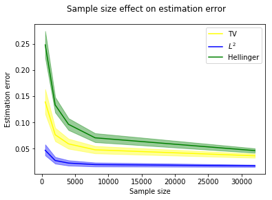
Figure 3: Estimation error of $\bar{\boldsymbol{X}}_{n}$ measured by total variation, Hellinger, and $\mathbb{L}^{2}$ distances as a function of (left panel) number of observations with contamination rate 0.2 and dimension $10^{2}$ and (right panel) dimension with contamination rate 0.2 and $10^{4}$ samples. The interval between 5th and 95th quantiles of the error, obtained from $10^{4}$ repetitions, is also depicted for every graph.

The error of $\bar{X}_{n}$ as a function of the sample size $n$, dimension $k$, and contamination rate $\varepsilon$ is plotted in Figures 3 and 4. These plots are conform to the theoretical results. Indeed, the first plot in Figure 3 shows that the errors for the three distances is decreasing w.r.t.  $n$. Furthermore, we see that up to some level of $n$ this decay is of order $n^{-1/2}$. The second plot in Figure 3 confirms that the risk grows linearly in $k$ for the TV and Hellinger distances, while it is constant for the $\mathbb{L}^{2}$ error.

Left panel of Figure 4 suggests that the error grows linearly in terms of contamination rate. This is conform to our results for the TV and $\mathbb{L}^{2}$ errors. But it might seem that there is a disagreement with the result for the Hellinger distance, for which the risk is shown to increase at the rate $\varepsilon^{1/2}$ and not $\varepsilon$. This is explained by the fact that the rate $\varepsilon^{1/2}$ corresponds to the worst-case risk, whereas here, the setting under experiment does not necessarily represent the worst case. When the parameter vectors of the reference and contamination distributions, respectively, are $\boldsymbol{e}_{i}$ and $\boldsymbol{e}_{j}$ with $i\neq j$ (i.e., when these two distributions are at the largest possible distance, which we call an extreme case), the graph of the error as a function of $\varepsilon$ (right panel of Figure 4) is similar to that of square-root function.

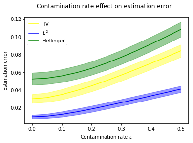
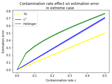
Figure 4: The estimation error of $\bar{\boldsymbol{X}}_{n}$ measured by total variation, Hellinger, and $\mathbb{L}^{2}$ distances in terms of the contamination rate (with dimension $10^{2}$ and $10^{4}$ samples). At right, we plotted the error with respect to the contamination rate for an extreme case, where the reference and contamination distributions have the largest distance. The interval between 5th and 95th quantiles of the error, obtained from $10^{4}$ trials, is also depicted.

6 Summary and conclusion

We have analyzed the problem of robust estimation of the mean of a random vector belonging to the probability simplex. Four measures of accuracy have been considered: total variation, Hellinger, Euclidean and Wasserstein distances. In each case, we have established the minimax rates of the expected error of estimation under the sparsity assumption. In addition, confidence regions shrinking at the minimax rate have been proposed.

An intriguing observation is that the choice of the distance has much stronger impact on the rate than the nature of contamination. Indeed, while the rates for the aforementioned distances are all different, the rate corresponding to one particular distance is not sensitive to the nature of outliers (ranging from Huber’s contamination to the adversarial one). While the rate obtained for the TV-distance coincides with the previously known rate of robustly estimating a Gaussian mean, the rates we have established for the Hellinger and for the Euclidean distances appear to be new. Interestingly, when the error is measured by the Euclidean distance, the quality of estimation does not get deteriorated with increasing dimension.

Appendix A Proofs of propositions

Proof A.1 (Proof of Proposition LABEL:prop@1 on page 1).

Recall that $\widehat{O}$ is the set of outliers in the Huber model. Let $O$ be any subset of $\{1,\ldots,n\}$. It follows from the definition of Huber’s model that if $\boldsymbol{P}_{n}^{O}$ stands for the conditional distribution of $(\boldsymbol{X}_{1},\ldots,\boldsymbol{X}_{n})$ given $\widehat{O}=O$, when $(\boldsymbol{X}_{1},\ldots,\boldsymbol{X}_{n})$ is drawn from $\boldsymbol{P}^{n}\in\mathcal{M}_{n}^{\text{HC}}(\varepsilon,\boldsymbol{\theta}^{*})$, then $\boldsymbol{P}_{n}^{O}\in\mathcal{M}_{n}^{\text{HDC}}(|O|/n,\boldsymbol{\theta}^{*})$. Therefore, for every $O$ of cardinality $o\geq 2\varepsilon n$, we have

$$\sup_{\mathcal{M}_{n}^{\text{HC}}(\varepsilon,\boldsymbol{\theta}^{*})}\mathbf{E}[d(\widehat{\boldsymbol{\theta}}_{n},\boldsymbol{\theta}^{*})\mathds{1}(\widehat{O}=O)] =\sup_{\mathcal{M}_{n}^{\text{HC}}(\varepsilon,\boldsymbol{\theta}^{*})}\mathbf{E}[d(\widehat{\boldsymbol{\theta}}_{n},\boldsymbol{\theta}^{*})|\widehat{O}=O]\mathbf{P}(\widehat{O}=O)$$ (35)

$$\stackrel{{\scriptstyle}}{{\leq}}\sup_{\mathcal{M}_{n}^{\text{HDC}}(o/n,\boldsymbol{\theta}^{*})}\mathbf{E}[d(\widehat{\boldsymbol{\theta}}_{n},\boldsymbol{\theta}^{*})]\mathbf{P}(\widehat{O}=O)$$ (36)

$$\stackrel{{\scriptstyle(1)}}{{\leq}}\sup_{\mathcal{M}_{n}^{\text{HDC}}(1,\boldsymbol{\theta}^{*})}\mathbf{E}[d(\widehat{\boldsymbol{\theta}}_{n},\boldsymbol{\theta}^{*})]\mathbf{P}(\widehat{O}=O).$$ (37)

Inequality (1) above is a direct consequence of the inclusion $\mathcal{M}_{n}^{\text{HDC}}(o/n,\boldsymbol{\theta}^{*})\subset\mathcal{M}_{n}^{\text{HDC}}(1,\boldsymbol{\theta}^{*})$. Summing the obtained inequality over all sets $O$ of cardinality $\geq 2\varepsilon n$, we get

$$\sup_{\mathcal{M}_{n}^{\text{HC}}(\varepsilon,\boldsymbol{\theta}^{*})}\mathbf{E}[d(\widehat{\boldsymbol{\theta}}_{n},\boldsymbol{\theta}^{*})\mathds{1}(|\widehat{O}|\geq 2\varepsilon n)] \leq\sup_{\mathcal{M}_{n}^{\text{HDC}}(1,\boldsymbol{\theta}^{*})}\mathbf{E}[d(\widehat{\boldsymbol{\theta}}_{n},\boldsymbol{\theta}^{*})]\mathbf{P}(|\widehat{O}|\geq 2\varepsilon n).$$ (38)

It follows from the multiplicative form of Chernoff’s inequality that $\mathbf{P}(|\widehat{O}|\geq 2\varepsilon n)\leq e^{-n\varepsilon/3}$. This leads to the last term in inequality (11).

Using the same argument as for (36), for any $O$ of cardinality $o<2n\varepsilon$, we get

$$\sup_{\mathcal{M}_{n}^{\text{HC}}(\varepsilon,\boldsymbol{\theta}^{*})}\mathbf{E}[d(\widehat{\boldsymbol{\theta}}_{n},\boldsymbol{\theta}^{*})\mathds{1}(|\widehat{O}|<2n\varepsilon)] \leq\sup_{\mathcal{M}_{n}^{\text{HDC}}(2\varepsilon,\boldsymbol{\theta}^{*})}\mathbf{E}[d(\widehat{\boldsymbol{\theta}}_{n},\boldsymbol{\theta}^{*})]\sum_{O:|O|\leq 2n\varepsilon}\mathbf{P}(\widehat{O}=O)$$ (39)

$$=\sup_{\mathcal{M}_{n}^{\text{HDC}}(2\varepsilon,\boldsymbol{\theta}^{*})}\mathbf{E}[d(\widehat{\boldsymbol{\theta}}_{n},\boldsymbol{\theta}^{*})].$$ (40)

This completes the proof of (11).

One can use the same arguments along with the Tchebychev inequality to establish (12). Indeed, for every $S$ of cardinality $o\leq 2\varepsilon n$, we have

$$\sup_{\mathcal{M}_{n}^{\text{HC}}(\varepsilon,\boldsymbol{\theta}^{*})}r\mathbf{P}\big{(}d(\widehat{\boldsymbol{\theta}}_{n},\boldsymbol{\theta}^{*}) >r\ \text{and}\ \widehat{O}=O\big{)}$$ (41)

$$=\sup_{\mathcal{M}_{n}^{\text{HC}}(\varepsilon,\boldsymbol{\theta}^{*})}r\mathbf{P}\big{(}d(\widehat{\boldsymbol{\theta}}_{n},\boldsymbol{\theta}^{*})>r\,|\,\widehat{O}=O\big{)}\mathbf{P}(\widehat{O}=O)$$ (42)

$$\stackrel{{\scriptstyle}}{{\leq}}\sup_{\mathcal{M}_{n}^{\text{HDC}}(o/n,\boldsymbol{\theta}^{*})}r\mathbf{P}\big{(}d(\widehat{\boldsymbol{\theta}}_{n},\boldsymbol{\theta}^{*})>r\big{)}\mathbf{P}(\widehat{O}=O)$$ (43)

$$\stackrel{{\scriptstyle}}{{\leq}}\sup_{\mathcal{M}_{n}^{\text{HDC}}(2\varepsilon,\boldsymbol{\theta}^{*})}\mathbf{E}[d(\widehat{\boldsymbol{\theta}}_{n},\boldsymbol{\theta}^{*})]\mathbf{P}(\widehat{O}=O).$$ (44)

Summing the obtained inequality over all sets $O$ of cardinality $o\leq 2\varepsilon n$, we get

$$\sup_{\mathcal{M}_{n}^{\text{HC}}(\varepsilon,\boldsymbol{\theta}^{*})}r\mathbf{P}\big{(}d(\widehat{\boldsymbol{\theta}}_{n},\boldsymbol{\theta}^{*})>r\ \text{and}\ |\widehat{O}|\leq 2\varepsilon n\big{)} \stackrel{{\scriptstyle}}{{\leq}}\sup_{\mathcal{M}_{n}^{\text{HDC}}(2\varepsilon,\boldsymbol{\theta}^{*})}\mathbf{E}[d(\widehat{\boldsymbol{\theta}}_{n},\boldsymbol{\theta}^{*})]$$ (45)

$$=R_{d}^{\text{HDC}}(n,2\varepsilon,\boldsymbol{\theta}^{*},\widehat{\boldsymbol{\theta}}).$$ (46)

On the other hand, it holds that

$$\sup_{\mathcal{M}_{n}^{\text{HC}}(\varepsilon,\boldsymbol{\theta}^{*})}r\mathbf{P}\big{(}d(\widehat{\boldsymbol{\theta}}_{n},\boldsymbol{\theta}^{*}) >r\ \text{and}\ |\widehat{O}|>2\varepsilon n\big{)}\stackrel{{\scriptstyle}}{{\leq}}r\mathbf{P}\big{(}|\widehat{O}|>2\varepsilon n)\leq re^{-n\varepsilon/3},$$ (47)

and the claim of the proposition follows.

Proof A.2 (Proof of Proposition LABEL:prop@2 on page 2).

Let $\boldsymbol{\theta}_{1}$ and $\boldsymbol{\theta}_{2}$ be two points in $\Theta$. We have

$$2R_{d}^{\text{HC}}(n,\varepsilon,\Theta,\widehat{\boldsymbol{\theta}}_{n}) \geq R_{d}^{\text{HC}}(n,\varepsilon,\boldsymbol{\theta}_{1},\widehat{\boldsymbol{\theta}}_{n})+R_{d}^{\text{HC}}(n,\varepsilon,\boldsymbol{\theta}_{2},\widehat{\boldsymbol{\theta}}_{n})$$ (48)

$$\geq\mathbf{E}_{(1-\varepsilon)\boldsymbol{P}_{\boldsymbol{\theta}_{1}}+\varepsilon\boldsymbol{P}_{\boldsymbol{\theta}_{2}}}[d(\widehat{\boldsymbol{\theta}}_{n},\boldsymbol{\theta}_{1})]+\mathbf{E}_{(1-\varepsilon)\boldsymbol{P}_{\boldsymbol{\theta}_{1}}+\varepsilon\boldsymbol{P}_{\boldsymbol{\theta}_{2}}}[d(\widehat{\boldsymbol{\theta}}_{n},\boldsymbol{\theta}_{2})].$$ (49)

To ease writing, assume that $n$ is an even number. Let $O$ be any fixed set of cardinality $n/2$. It is clear that the set of outliers $\widehat{O}$ satisfies

$$p_{O}=\boldsymbol{P}(\widehat{O}=O)=\boldsymbol{P}(\widehat{O}=O^{c})>0.$$

Furthermore, if $\boldsymbol{X}_{1:n}$ is drawn from $((1-\varepsilon)\boldsymbol{P}_{\boldsymbol{\theta}_{1}}+\varepsilon\boldsymbol{P}_{\boldsymbol{\theta}_{2}})^{\otimes n}$, then its conditional distribution given $\widehat{O}=O$ is exactly the same as the conditional distribution of $\boldsymbol{X}_{1:n}\sim((1-\varepsilon)\boldsymbol{P}_{\boldsymbol{\theta}_{2}}+\varepsilon\boldsymbol{P}_{\boldsymbol{\theta}_{1}})^{\otimes n}$ given $\widehat{O}=O^{c}$. This implies that

$$2R_{d}^{\text{HC}} (n,\varepsilon,\Theta,\widehat{\boldsymbol{\theta}}_{n})$$ (50)

$$\geq p_{O}\big{(}\mathbf{E}_{(1-\varepsilon)\boldsymbol{P}_{\boldsymbol{\theta}_{1}}+\varepsilon\boldsymbol{P}_{\boldsymbol{\theta}_{2}}}[d(\widehat{\boldsymbol{\theta}}_{n},\boldsymbol{\theta}_{1})|\widehat{O}=O]+\mathbf{E}_{(1-\varepsilon)\boldsymbol{P}_{\boldsymbol{\theta}_{1}}+\varepsilon\boldsymbol{P}_{\boldsymbol{\theta}_{2}}}[d(\widehat{\boldsymbol{\theta}}_{n},\boldsymbol{\theta}_{2})|\widehat{O}=O^{c}]\big{)}$$ (51)

$$=p_{O}\mathbf{E}_{(1-\varepsilon)\boldsymbol{P}_{\boldsymbol{\theta}_{1}}+\varepsilon\boldsymbol{P}_{\boldsymbol{\theta}_{2}}}[d(\widehat{\boldsymbol{\theta}}_{n},\boldsymbol{\theta}_{1})+d(\widehat{\boldsymbol{\theta}}_{n},\boldsymbol{\theta}_{2})|\widehat{O}=S]\geq p_{O}d(\boldsymbol{\theta}_{1},\boldsymbol{\theta}_{2}),$$ (52)

where in the last step we have used the triangle inequality. The obtained inequality being true for every $\boldsymbol{\theta}_{1},\boldsymbol{\theta}_{2}\in\Theta$, we can take the supremum to get

$$R_{d}^{\text{HC}}(n,\varepsilon,\Theta,\widehat{\boldsymbol{\theta}}_{n}) \geq(p_{O}/2)\sup_{\boldsymbol{\theta}_{1},\boldsymbol{\theta}_{2}\in\Theta}d(\boldsymbol{\theta}_{1},\boldsymbol{\theta}_{2})=+\infty.$$ (53)

This completes the proof.

Appendix B Upper bounds on the minimax risk over the sparse simplex

This section is devoted to the proof of the upper bounds on minimax risks in the discrete model with respect to various distances.

Proof B.1 (Proof of Theorem LABEL:theorem@1 on page 3).

To ease notation, we set

$$\bar{\boldsymbol{X}}_{n}=\frac{1}{n}\sum_{i}\boldsymbol{X}_{i},\quad\bar{\boldsymbol{Y}}_{n}=\frac{1}{n}\sum_{i}\boldsymbol{Y}\!_{i},\quad\bar{\boldsymbol{X}}_{O}=\frac{1}{o}\sum_{i\in O}\boldsymbol{X}_{i},\quad\bar{\boldsymbol{Y}}_{O}=\frac{1}{o}\sum_{i\in O}\boldsymbol{Y}\!_{i}$$ (54)

In the adversarial model, we have $\boldsymbol{X}_{i}=\boldsymbol{Y}\!_{i}$ if $i\not\in O$ where $\boldsymbol{Y}\!_{1},\dots,\boldsymbol{Y}\!_{n}$ are generated from the reference distribution $\boldsymbol{\theta}^{*}$.

$$d_{\mathbb{L}^{2}}(\bar{\boldsymbol{X}}_{n},\boldsymbol{\theta}^{*}) =\big{\|}\bar{\boldsymbol{X}}_{n}-\boldsymbol{\theta}^{*}\big{\|}_{2}=\big{\|}\bar{\boldsymbol{Y}}_{n}-\boldsymbol{\theta}^{*}+\frac{1}{n}\sum_{i\in O}(\boldsymbol{X}_{i}-\boldsymbol{Y}\!_{i})\big{\|}_{2}$$ (55)

$$\leq\big{\|}\bar{\boldsymbol{Y}}_{n}-\boldsymbol{\theta}^{*}\big{\|}_{2}+\frac{|O|}{n}\sup_{\boldsymbol{x},\boldsymbol{y}\in\Delta^{k-1}}\|\boldsymbol{x}-\boldsymbol{y}\|_{2}$$ (56)

$$=\big{\|}\bar{\boldsymbol{Y}}_{n}-\boldsymbol{\theta}^{*}\big{\|}_{2}+\sqrt{2}\varepsilon,$$ (57)

which gives us

$$\sup_{\mathcal{M}_{n}^{\rm AC}(\varepsilon,\boldsymbol{\theta}^{*})}\mathbf{E}[d_{\mathbb{L}^{2}}(\bar{\boldsymbol{X}}_{n},\boldsymbol{\theta}^{*})] \leq\ \sup_{\boldsymbol{\theta}^{*}}\mathbf{E}[d_{\mathbb{L}^{2}}(\bar{\boldsymbol{Y}}_{n},\boldsymbol{\theta}^{*})]+\sqrt{2}\varepsilon.$$ (58)

And for a fixed $\boldsymbol{\theta}^{*}$ it is well known that

$$\mathbf{E}[d^{2}_{\mathbb{L}^{2}}(\bar{\boldsymbol{Y}}_{n},\boldsymbol{\theta}^{*})] =\sum_{j=1}^{k}\mathbf{Var}[\bar{\boldsymbol{Y}}_{n,j}]=\sum_{j=1}^{k}\mathbf{Var}\bigg{[}\frac{1}{n}\sum_{i=1}^{n}\mathds{1}(Y_{i}=\boldsymbol{e}_{j})\bigg{]}$$ (59)

$$=\frac{1}{n}\sum_{j=1}^{k}\mathbf{Var}[\mathds{1}(Y_{1}=\boldsymbol{e}_{j})]$$ (60)

$$\leq\frac{1}{n}\sum_{j=1}^{k}\mathbf{E}[\mathds{1}(Y_{1}=\boldsymbol{e}_{j})]=\frac{1}{n}.$$ (61)

Hence, we obtain $R_{\rm\mathbb{L}^{2}}^{\rm AC}(n,\varepsilon,\Delta^{k-1})\leq(1/n)^{1/2}+\varepsilon$. Similarly,

$$d_{\rm TV}(\bar{\boldsymbol{X}}_{n},\boldsymbol{\theta}^{*}) \leq\big{\|}\bar{\boldsymbol{Y}}_{n}-\boldsymbol{\theta}^{*}\big{\|}_{1}+\frac{|O|}{n}\sup_{\boldsymbol{x},\boldsymbol{y}\in\Delta^{k-1}}\|\boldsymbol{x}-\boldsymbol{y}\|_{1}$$ (62)

$$=\big{\|}\bar{\boldsymbol{Y}}_{n}-\boldsymbol{\theta}^{*}\big{\|}_{1}+2\varepsilon.$$ (63)

This gives

$$\sup_{\mathcal{M}_{n}^{\rm AC}(\varepsilon,\boldsymbol{\theta}^{*})}\mathbf{E}[d_{\rm TV}(\bar{\boldsymbol{X}}_{n},\boldsymbol{\theta}^{*})] \leq\ \sup_{\boldsymbol{\theta}^{*}}\mathbf{E}[d_{\rm TV}(\bar{\boldsymbol{Y}}_{n},\boldsymbol{\theta}^{*})]+2\varepsilon.$$ (64)

In addition, for every $\boldsymbol{\theta}^{*}$,

$$\mathbf{E}[d_{\rm TV}(\bar{\boldsymbol{Y}}_{n},\boldsymbol{\theta}^{*})] =\frac{1}{2}\sum_{j=1}^{k}\mathbf{E}\big{[}\big{|}\bar{\boldsymbol{Y}}_{n,j}-\boldsymbol{\theta}^{*}_{j}\big{|}\big{]}$$ (65)

$$\leq\frac{1}{2}\sum_{j=1}^{k}\bigg{(}\mathbf{E}\big{[}\big{|}\bar{\boldsymbol{Y}}_{n,j}-\boldsymbol{\theta}^{*}_{j}\big{|}^{2}\big{]}\bigg{)}^{1/2}$$ (66)

$$=\frac{1}{2}\sum_{j=1}^{k}\bigg{(}\mathbf{Var}\big{[}\bar{\boldsymbol{Y}}_{n,j}\big{]}\bigg{)}^{1/2}$$ (67)

$$\stackrel{{\scriptstyle(1)}}{{=}}\frac{1}{2}\sum_{j\in J}\big{(}\frac{1}{n}\boldsymbol{\theta}^{*}_{j}(1-\boldsymbol{\theta}^{*}_{j})\big{)}^{1/2}$$ (68)

$$\stackrel{{\scriptstyle(2)}}{{\leq}}\frac{1}{2}\,s^{1/2}\bigg{(}\sum_{j=1}^{k}\frac{1}{n}\boldsymbol{\theta}^{*}_{j}(1-\boldsymbol{\theta}^{*}_{j})\bigg{)}^{1/2}$$ (69)

$$\leq\frac{1}{2}\big{(}{s}/n\big{)}^{1/2},$$ (70)

where in (1) we have used the notation $J=\{j:\theta_{j}^{*}\neq 0\}$ and in (2) we have used the Cauchy-Schwarz inequality. This leads to

$$R_{\rm TV}^{\rm AC}(n,\varepsilon,\Delta^{k-1})\leq(k/n)^{1/2}+\varepsilon.$$ (71)

Finally, for the Hellinger distance

$$d_{\rm H}(\bar{\boldsymbol{X}}_{n},\boldsymbol{\theta}^{*}) \leq d_{\rm H}(\bar{\boldsymbol{X}}_{n},\bar{\boldsymbol{Y}}_{n})+d_{\rm H}(\bar{\boldsymbol{Y}}_{n},\boldsymbol{\theta}^{*})\leq\sqrt{2}d_{\rm TV}(\bar{\boldsymbol{X}}_{n},\bar{\boldsymbol{Y}}_{n})^{1/2}+d_{\rm H}(\bar{\boldsymbol{Y}}_{n},\boldsymbol{\theta}^{*}),$$ (72)

where we have already seen that

$$d_{\rm TV}(\bar{\boldsymbol{X}}_{n},\bar{\boldsymbol{Y}}_{n}) =\frac{o}{n}\big{\|}\bar{\boldsymbol{X}}_{O}-\bar{\boldsymbol{Y}}_{O}\big{\|}_{1}\leq 2\varepsilon.$$ (73)

This yields

$$\sup_{\mathcal{M}_{n}^{\rm AC}(\varepsilon,\boldsymbol{\theta}^{*})}\mathbf{E}[d_{\rm H}(\bar{\boldsymbol{X}}_{n},\boldsymbol{\theta}^{*})] \leq\ \sup_{\boldsymbol{\theta}^{*}}\mathbf{E}[d_{\rm H}(\bar{\boldsymbol{Y}}_{n},\boldsymbol{\theta}^{*})]+2\sqrt{\varepsilon}.$$ (74)

Furthermore, for every $\boldsymbol{\theta}^{*}\in\Delta^{k-1}_{s}$,

$$\mathbf{E}[d^{2}_{\rm H}(\bar{\boldsymbol{Y}}_{n},\boldsymbol{\theta}^{*})] =\mathbf{E}\bigg{[}\sum_{j=1}^{k}\Big{(}\sqrt{\bar{\boldsymbol{Y}}_{n,j}}-\sqrt{\boldsymbol{\theta}^{*}_{j}}\Big{)}^{2}\bigg{]}$$ (75)

$$\leq\mathbf{E}\bigg{[}\sum_{j\in J}\frac{(\bar{\boldsymbol{Y}}_{n,j}-\boldsymbol{\theta}^{*}_{j})^{2}}{\boldsymbol{\theta}^{*}_{j}}\bigg{]}$$ (76)

$$=\sum_{j\in J}\frac{1}{\boldsymbol{\theta}^{*}_{j}}\mathbf{Var}\big{[}{\bar{\boldsymbol{Y}}_{n,j}}\big{]}=\sum_{j\in J}\frac{1}{\boldsymbol{\theta}^{*}_{j}}\frac{\boldsymbol{\theta}^{*}_{j}(1-\boldsymbol{\theta}^{*}_{j})}{n}=\frac{s-1}{n}.$$ (77)

Hence, by Jensen’s inequality $\mathbf{E}[d_{\rm H}(\bar{\boldsymbol{Y}}_{n},\boldsymbol{\theta}^{*})]<\sqrt{s/n}$. Therefore, we infer that

$$R_{\rm H}^{\rm AC}(n,\varepsilon,\Delta_{s}^{k-1})\leq(s/n)^{1/2}+2\varepsilon^{1/2}$$ (78)

and the last claim of the theorem follows.

Appendix C Lower bounds on the minimax risk over the sparse simplex

This section is devoted to the proof of the lower bounds on minimax risks in the discrete model with respect to various distances. Note that the rates over the high-dimensional “sparse” simplex $\Delta^{k-1}_{s}$ coincide with those for the dense simplex $\Delta^{s-1}$. For this reason, all the lower bounds will be proved for $\Delta^{s-1}$ only (for $s\geq 2$ an even integer). In addition, we will restrict our attention to the distributions $\boldsymbol{P}$, $\boldsymbol{Q}$ over $\Delta^{s-1}$ that are supported by the set $\mathcal{A}$ of the elements of the canonical basis that is $\boldsymbol{P}(\mathcal{A})=\boldsymbol{Q}(\mathcal{A})=1$.

Proof C.1 (Proof of Theorem LABEL:theorem@2 on page 4).

We denote by $\boldsymbol{e}_{j}$ the vector in $\mathbb{R}^{s}$ having all the coordinates equal to zero except the $j$th coordinate which is equal to one. Setting

$$\boldsymbol{\theta}=\boldsymbol{e}_{1},\quad\text{and}\quad\boldsymbol{\theta}^{\prime}=\Big{(}1-\frac{\varepsilon}{1-\varepsilon}\Big{)}\boldsymbol{e}_{1}+\frac{\varepsilon}{1-\varepsilon}\boldsymbol{e}_{2}$$ (79)

we have

$$d_{\rm TV}(\boldsymbol{\theta},\boldsymbol{\theta}^{\prime})=\frac{\varepsilon}{1-\varepsilon},\quad d_{\mathbb{L}^{2}}(\boldsymbol{\theta},\boldsymbol{\theta}^{\prime})\geq\sqrt{2}\varepsilon,\quad\text{and}\quad d_{\rm H}(\boldsymbol{\theta},\boldsymbol{\theta}^{\prime})\geq(\varepsilon/2)^{1/2}.$$ (80)

Therefore, modulus of continuity defined by

$$w_{d}(\varepsilon,\Delta)=\sup\big{\{}d(\boldsymbol{\theta},\boldsymbol{\theta}^{\prime}):\boldsymbol{\theta},\boldsymbol{\theta}^{\prime}\in\Delta,\ d_{\text{TV}}(\boldsymbol{\theta},\boldsymbol{\theta}^{\prime})\leq\varepsilon/(1-\varepsilon)\big{\}}$$

for a distance $d$ and a set $\Delta$, satisfies for any $\varepsilon\leq 1/2$,

$$w_{\rm TV}(\varepsilon,\Delta^{k-1})\geq\varepsilon,\quad w_{\mathbb{L}^{2}}(\varepsilon,\Delta^{k-1})\geq\sqrt{2}\varepsilon,\quad\text{and}\quad w_{\rm H}(\varepsilon,\Delta^{k-1})\geq(\varepsilon/2)^{1/2}.$$ (81)

These bounds on the modulus of continuity are the first ingredient we need to be able to apply Theorem 5.1 from (Chen et al., 2018) for getting minimax lower bounds.

The second ingredient is the minimax rate in the non-contaminated case. are well known. For each of the considered distances, this rate is well-known. However, for the sake of completeness, we provide below a proof those lower bounds using Fano’s method. For this, we use the Varshamov-Gilbert lemma (see e.g. Lemma 2.9 in (Tsybakov, 2009)) and Theorem 2.5 in (Tsybakov, 2009). The Varshamov-Gilbert lemma guarantees the existence of a set ${\boldsymbol{\omega}}^{(1)},\dots,{\boldsymbol{\omega}}^{(M)}\in\{0,1\}^{\lfloor s/2\rfloor}$ of cardinality $M\geq 2^{s/16}$ such that

$$\rho({\boldsymbol{\omega}}^{(i)},{\boldsymbol{\omega}}^{(j)})\geq\frac{s}{16},\quad\text{for all}\quad i\neq j,$$ (82)

where $\rho(.,.)$ stands for the Hamming distance. Using these binary vectors $\{\boldsymbol{\omega}_{j}\}$, a parameter $\beta\in[0,\sqrt{n/s}]$ to be specified later and the “baseline” vector $\boldsymbol{\theta}^{(0)}=(1/s,\dots,1/s)$, we define hypotheses $\boldsymbol{\theta}^{(1)}$, $\dots$, $\boldsymbol{\theta}^{(M)}$ by the relations

$$\boldsymbol{\theta}^{(i)}_{2j-1}=\boldsymbol{\theta}^{(0)}_{2j-1}+{\boldsymbol{\omega}}^{(i)}_{j}\frac{\beta}{\sqrt{ns}}\quad\text{ and }\quad\boldsymbol{\theta}^{(i)}_{2j}=\boldsymbol{\theta}^{(0)}_{2j}-{\boldsymbol{\omega}}^{(i)}_{j}\frac{\beta}{\sqrt{ns}}\quad\forall j\in\{0,\dots,\lfloor s/2\rfloor\}.$$ (83)

Remark that $\boldsymbol{\theta}^{(0)},\dots,\boldsymbol{\theta}^{(M)}$ are all probability vectors of dimension $s$. Denoting the Kullback-Leibler divergence by $d_{\rm KL}(.,.)$, one can check the conditions of Theorem 2.5 in Tsybakov (2009):

$$d_{\mathbb{L}^{2}}(\boldsymbol{\theta}^{(i)},\boldsymbol{\theta}^{(j)}) \geq\sqrt{2}\frac{\beta}{\sqrt{ns}}\frac{\sqrt{s}}{4}=\frac{\beta}{\sqrt{8n}}\qquad\forall j\neq i,$$ (84)

$$d_{\rm TV}(\boldsymbol{\theta}^{(i)},\boldsymbol{\theta}^{(j)}) \geq\frac{\beta}{\sqrt{ns}}\frac{s}{16}=\frac{\beta\sqrt{s}}{16\sqrt{n}}\qquad\forall j\neq i,$$ (85)

as well as

$$d_{\rm KL}(\boldsymbol{\theta}^{(i)},\boldsymbol{\theta}^{(0)}) \leq\sum_{j=1}^{\lfloor s/2\rfloor}\log\frac{\boldsymbol{\theta}^{(0)}_{2j-1}+\frac{\beta}{\sqrt{ns}}}{\boldsymbol{\theta}^{(0)}_{2j-1}}(\boldsymbol{\theta}^{(0)}_{2j-1}+\frac{\beta}{\sqrt{ns}})+\log\frac{\boldsymbol{\theta}^{(0)}_{2j}-\frac{\beta}{\sqrt{ns}}}{\boldsymbol{\theta}^{(0)}_{2j}}(\boldsymbol{\theta}^{(0)}_{2j}-\frac{\beta}{\sqrt{ns}})$$ (86)

$$\leq\sum_{j=1}^{\lfloor k/2\rfloor}\frac{\beta}{\sqrt{ns}\boldsymbol{\theta}^{(0)}_{2j-1}}(\boldsymbol{\theta}^{(0)}_{2j-1}+\frac{\beta}{\sqrt{ns}})-\frac{\beta}{\sqrt{ns}\boldsymbol{\theta}^{(0)}_{2j}}(\boldsymbol{\theta}^{(0)}_{2j}-\frac{\beta}{\sqrt{ns}})$$ (87)

$$=\frac{\beta^{2}}{ns}\sum_{j=1}^{k}\frac{1}{\boldsymbol{\theta}^{(0)}_{j}}=\frac{\beta^{2}}{ns}\sum_{j=1}^{s}s=\frac{\beta^{2}s}{n}\leq\frac{\alpha\log M}{n}\qquad\forall i\in\{1,\dots,M\},$$ (88)

for $\beta=\sqrt{\alpha}/4$. Now by applying the aforementioned theorem, we obtain for the non-contaminated setting ($\varepsilon=0$)

$$\inf_{\bar{\boldsymbol{\theta}_{n}}}\sup_{\mathcal{M}_{n}^{\rm HC}(0,\Delta^{s-1})}\boldsymbol{P}\bigg{(}d_{\mathbb{L}^{2}}(\bar{\boldsymbol{\theta}}_{n},{\boldsymbol{\theta}}^{*})\geq\frac{\beta}{\sqrt{2n}}\bigg{)}\geq\frac{\sqrt{M}}{1+\sqrt{M}}\bigg{(}1-2\alpha-\sqrt{\frac{2\alpha}{\log M}}\bigg{)},$$ (89)

$$\inf_{\bar{\boldsymbol{\theta}_{n}}}\sup_{\mathcal{M}_{n}^{\rm HC}(0,\Delta^{s-1})}\boldsymbol{P}\bigg{(}d_{\rm TV}(\bar{\boldsymbol{\theta}}_{n},{\boldsymbol{\theta}}^{*})\geq\frac{\beta\sqrt{s}}{8\sqrt{n}}\bigg{)}\geq\frac{\sqrt{M}}{1+\sqrt{M}}\bigg{(}1-2\alpha-\sqrt{\frac{2\alpha}{\log M}}\bigg{)}.$$ (90)

Setting $M=2^{k/16}$ and $\alpha=1/32$, by Markov’s inequality, one concludes

$$\inf_{\bar{\boldsymbol{\theta}}_{n}}R_{\mathbb{L}^{2}}^{\text{HC}}(n,0,\Delta^{s-1},\bar{\boldsymbol{\theta}}_{n}) \geq c(1/n)^{1/2},$$ (91)

$$\inf_{\bar{\boldsymbol{\theta}}_{n}}R_{\rm TV}^{\text{HC}}(n,0,\Delta^{s-1},\bar{\boldsymbol{\theta}}_{n}) \geq c(s/n)^{1/2},$$ (92)

where $c=1/25600$. Since, $d_{\rm H}(\boldsymbol{\theta},\boldsymbol{\theta}^{\prime})\geq d_{\rm TV}(\boldsymbol{\theta},\boldsymbol{\theta}^{\prime})$ for any distribution $\boldsymbol{\theta}$ and $\boldsymbol{\theta}^{\prime}$

$$\inf_{\bar{\boldsymbol{\theta}}_{n}}R_{\rm H}^{\text{HC}}(n,0,\Delta^{s-1},\bar{\boldsymbol{\theta}}_{n}) \geq c(s/n)^{1/2}.$$ (93)

Finally, we apply (Chen et al., 2018, Theorem 5.1) stating in our case for any distance $d$

$$\inf_{\bar{\boldsymbol{\theta}}_{n}}R_{d}^{\text{HC}}(n,\varepsilon,\Delta^{s-1},\bar{\boldsymbol{\theta}}_{n}) \geq c\big{\{}\inf_{\bar{\boldsymbol{\theta}}_{n}}R_{d}^{\text{HC}}(n,0,\Delta^{s-1},\bar{\boldsymbol{\theta}}_{n})+w_{d}(\varepsilon,\Delta^{s-1})\big{\}},$$ (94)

for an universal constant $c$, which completes the proof of Theorem LABEL:theorem@2.

Appendix D Proofs of bounds with high probability

Proof D.1.

Suppose $\boldsymbol{X}_{i}=\boldsymbol{Y}\!_{i}$ if $i\not\in O$ where $\boldsymbol{Y}\!_{1},\dots,\boldsymbol{Y}\!_{n}$ are independently generated from the reference distribution $\boldsymbol{P}$ so that $\mathbf{E}[\boldsymbol{Y}\!_{i}]=\boldsymbol{\theta}^{*}$. For any $\boldsymbol{Z}_{1},\dots,\boldsymbol{Z}_{n}$, let $\boldsymbol{\Phi}_{\square}(\boldsymbol{Z}_{1},\dots,\boldsymbol{Z}_{n}):=d_{\square}(\sum_{i=1}^{n}\boldsymbol{Z}_{i}/n,\boldsymbol{\theta}^{*})$, where $\square$ refers here to the distances $\mathbb{L}^{2}$ or TV. Given $\boldsymbol{Y}\!^{\prime}_{1},\dots,\boldsymbol{Y}\!^{\prime}_{n}\in\Delta^{k-1}$ we have for every $i$

$$\boldsymbol{\Phi}_{\square}(\boldsymbol{Y}\!_{1},\dots,\boldsymbol{Y}\!_{i},\dots,\boldsymbol{Y}\!_{n})-\boldsymbol{\Phi}_{\square}(\boldsymbol{Y}\!_{1},\dots,\boldsymbol{Y}\!_{i-1},\boldsymbol{Y}\!^{\prime}_{i},\boldsymbol{Y}\!_{i+1},\dots,\boldsymbol{Y}\!_{n})\leq\frac{1}{n}d_{\square}(\boldsymbol{Y}\!_{i},\boldsymbol{Y}\!^{\prime}_{i}).$$

Furthermore, it can easily be shown that the last term is bounded by $\sqrt{2}/n$ and $2/n$ for the distances $\mathbb{L}^{2}$ and TV, respectively. By bounded difference inequality (see for example Theorem 6.2 of Boucheron et al. (2013)) with probability at least $1-\delta$

$$\boldsymbol{\Phi}_{\mathbb{L}^{2}}(\boldsymbol{Y}\!_{1},\dots,\boldsymbol{Y}\!_{n}) \leq\mathbf{E}\boldsymbol{\Phi}_{\mathbb{L}^{2}}(\boldsymbol{Y}\!_{1},\dots,\boldsymbol{Y}\!_{n})+\big{(}\log(1/\delta)/n\big{)}^{1/2}$$ (95)

$$\leq(1/n)^{1/2}+\big{(}\log(1/\delta)/n\big{)}^{1/2},$$ (96)

$$\boldsymbol{\Phi}_{TV}(\boldsymbol{Y}\!_{1},\dots,\boldsymbol{Y}\!_{n}) \leq\mathbf{E}\boldsymbol{\Phi}_{TV}(\boldsymbol{Y}\!_{1},\dots,\boldsymbol{Y}\!_{n})+\big{(}\log(2/\delta)/n\big{)}^{1/2}$$ (97)

$$\leq(s/n)^{1/2}+\big{(}\log(2/\delta)/n\big{)}^{1/2}.$$ (98)

Using $\boldsymbol{\Phi}_{\square}(\boldsymbol{X}_{1},\dots,\boldsymbol{X}_{n})\leq\boldsymbol{\Phi}_{\square}(\boldsymbol{Y}\!_{1},\dots,\boldsymbol{Y}\!_{n})+d_{\square}(\sum_{i\in O}\boldsymbol{X}_{i}/n,\sum_{i\in O}\boldsymbol{Y}\!_{i}/n)$, one can conclude the proof of the first two claims of the theorem.

For the Hellinger distance, the computations are more tedious. We have to separate the case of small $\theta^{*}_{j}$. To this end, let $J=\{j:0<\theta^{*}_{j}<(1/n)\log(2s/\delta)\}$ and $J^{\prime}=\{j:\theta^{*}_{j}\geq(1/n)\log(2s/\delta)\}$. We have

$$\sum_{j\in J}\Big{(}\sqrt{\bar{\boldsymbol{Y}}\!_{n,j}}-\sqrt{\theta^{*}_{j}}\Big{)}^{2} \leq\sum_{j\in J}(\bar{\boldsymbol{Y}}\!_{n,j}+\theta^{*}_{j})$$ (99)

$$\leq\frac{1}{n}\sum_{i=1}^{n}\Big{(}\sum_{j\in J}\boldsymbol{Y}\!_{i,j}-\theta_{j}^{*}\Big{)}+\frac{2s\log(2s/\delta)}{n}.$$ (100)

Since the random variables $U_{i}:=\Big{(}\sum_{j\in J}\boldsymbol{Y}\!_{i,j}\Big{)}$ are iid, positive, bounded by $1$, the Bernstein inequality implies that

$$\frac{1}{n}\sum_{i=1}^{n}\big{(}U_{i}-\mathbf{E}[U_{1}]\big{)} \leq\sqrt{\frac{2\textbf{Var}(U_{1})\log(2/\delta)}{n}}+\frac{\log(2/\delta)}{3n},$$ (101)

holds with probability at least $1-\delta/2$ for $0<\delta<1$. One easily checks that $\sqrt{\textbf{Var}(U_{1})}\leq\sum_{j\in J}\sqrt{\textbf{Var}(\boldsymbol{Y}\!_{1,j})}\leq s\sqrt{\log(2s/\delta)/n}$. Therefore, with probability at least $1-\delta/2$, we have

$$\frac{1}{n}\sum_{i=1}^{n}\Big{(}\sum_{j\in J}\boldsymbol{Y}\!_{i,j}-\theta_{j}^{*}\Big{)} \leq\frac{\sqrt{2}\,s\log(2s/\delta)}{n}+{\frac{\log(2/\delta)}{3n}}.$$ (102)

This yields

$$\sum_{j\in J}\Big{(}\sqrt{\bar{\boldsymbol{Y}}\!_{n,j}}-\sqrt{\theta^{*}_{j}}\Big{)}^{2} \leq\frac{3.5s{\log(2s/\delta)}+\log(2/\delta)}{n},$$ (103)

with probability at least $1-\delta/2$.

On the other hand, we have

$$\sum_{j\in J^{\prime}}\Big{(}\sqrt{\bar{\boldsymbol{Y}}\!_{n,j}}-\sqrt{\theta^{*}_{j}}\Big{)}^{2} \leq\sum_{j\in J^{\prime}}\frac{(\bar{\boldsymbol{Y}}\!_{n,j}-\theta^{*}_{j})^{2}}{\theta_{j}^{*}}$$ (104)

$$\leq s\max_{j\in J^{\prime}}\frac{(\bar{\boldsymbol{Y}}\!_{n,j}-\theta^{*}_{j})^{2}}{\theta_{j}^{*}}.$$ (105)

The Bernstein inequality and the union bound imply that, with probability at least $1-\delta/2$,

$$|\bar{\boldsymbol{Y}}\!_{n,j}-\theta^{*}_{j}| \leq\sqrt{\frac{2\textbf{Var}(\boldsymbol{Y}\!_{1,j})\log(2s/\delta)}{n}}+\frac{\log(2s/\delta)}{n},\qquad\forall j\in J^{\prime}$$ (106)

$$\leq\sqrt{\frac{2\theta_{j}^{*}\log(2s/\delta)}{n}}+\frac{\log(2s/\delta)}{n},\qquad\forall j\in J^{\prime}$$ (107)

$$\leq 2.5\sqrt{\frac{\theta_{j}^{*}\log(2s/\delta)}{n}},\qquad\forall j\in J^{\prime}.$$ (108)

Combining (105) and (108), we obtain

$$\sum_{j\in J^{\prime}}\Big{(}\sqrt{\bar{\boldsymbol{Y}}\!_{n,j}}-\sqrt{\theta^{*}_{j}}\Big{)}^{2} \leq 2.5^{2}\frac{s\log(2s/\delta)}{n},$$ (109)

with probability at least $1-\delta/2$. Finally, inequalities (103) and (110) together lead to

$$d_{\textup{H}}^{2}(\bar{\boldsymbol{Y}}_{n},\boldsymbol{\theta}^{*})=\sum_{j=1}^{n}\Big{(}\sqrt{\bar{\boldsymbol{Y}}\!_{n,j}}-\sqrt{\theta^{*}_{j}}\Big{)}^{2} \leq\frac{9.75s\,\log(2s/\delta)}{n}+\frac{\log(2/\delta)}{n},$$ (110)

which is true with probability at least $1-\delta$. Using the triangle inequality and the fact that the Hellinger distance is smaller than the square root of the TV-distance, we get

$$d_{\textup{H}}(\bar{\boldsymbol{X}}_{n},\boldsymbol{\theta}^{*}) \leq d_{\textup{H}}(\bar{\boldsymbol{X}}_{n},\bar{\boldsymbol{Y}}_{n})+d_{\textup{H}}(\bar{\boldsymbol{Y}}_{n},\boldsymbol{\theta}^{*})$$ (111)

$$\leq\sqrt{2\,d_{\textup{TV}}(\bar{\boldsymbol{X}}_{n},\bar{\boldsymbol{Y}}_{n})}+d_{\textup{H}}(\bar{\boldsymbol{Y}}_{n},\boldsymbol{\theta}^{*})$$ (112)

$$\leq(2\varepsilon)^{1/2}+3.2\sqrt{\frac{s\,\log(2s/\delta)}{n}}+\sqrt{\frac{\log(2/\delta)}{n}},$$ (113)

with probability at least $1-\delta$. This completes the proof of the theorem.

References

- Audibert and Catoni (2011) J.-Y. Audibert and O. Catoni. Robust linear least squares regression. Ann. Statist., 39(5):2766–2794, 10 2011.
- Balakrishnan et al. (2017) S. Balakrishnan, S. S. Du, J. Li, and A. Singh. Computationally efficient robust sparse estimation in high dimensions. In Proceedings of the 30th Conference on Learning Theory, COLT 2017, Amsterdam, The Netherlands, 7-10 July 2017, pages 169–212, 2017.
- Bhatia et al. (2017) K. Bhatia, P. Jain, P. Kamalaruban, and P. Kar. Consistent robust regression. pages 1–18, December 2017.
- Boucheron et al. (2013) S. Boucheron, G. Lugosi, and P. Massart. Concentration Inequalities: A Nonasymptotic Theory of Independence. OUP Oxford, 2013.
- Carpentier et al. (2018) A. Carpentier, S. Delattre, E. Roquain, and N. Verzelen. Estimating minimum effect with outlier selection. arXiv e-prints, art. arXiv:1809.08330, Sept. 2018.
- Chen et al. (2016) M. Chen, C. Gao, and Z. Ren. A general decision theory for Huber’s -contamination model. Electronic Journal of Statistics, 10(2):3752–3774, 2016.
- Chen et al. (2018) M. Chen, C. Gao, and Z. Ren. Robust covariance and scatter matrix estimation under Huber’s contamination model. Ann. Statist., 46(5):1932–1960, 10 2018.
- Chen et al. (2013) Y. Chen, C. Caramanis, and S. Mannor. Robust sparse regression under adversarial corruption. In Proceedings of the 30th International Conference on Machine Learning, volume 28 of Proceedings of Machine Learning Research, pages 774–782. PMLR, 17–19 Jun 2013.
- Chinot et al. (2018) G. Chinot, G. Lecué, and M. Lerasle. Statistical learning with Lipschitz and convex loss functions. arXiv e-prints, art. arXiv:1810.01090, Oct. 2018.
- Collier and Dalalyan (2017) O. Collier and A. S. Dalalyan. Minimax estimation of a p-dimensional linear functional in sparse Gaussian models and robust estimation of the mean. arXiv e-prints, art. arXiv:1712.05495, Dec. 2017.
- Dalalyan and Chen (2012) A. Dalalyan and Y. Chen. Fused sparsity and robust estimation for linear models with unknown variance. In Advances in Neural Information Processing Systems 25, pages 1259–1267. Curran Associates, Inc., 2012.
- Devroye et al. (2016) L. Devroye, M. Lerasle, G. Lugosi, and R. I. Oliveira. Sub-gaussian mean estimators. Ann. Statist., 44(6):2695–2725, 12 2016.
- Diakonikolas et al. (2016) I. Diakonikolas, G. Kamath, D. M. Kane, J. Li, A. Moitra, and A. Stewart. Robust estimators in high dimensions without the computational intractability. In IEEE 57th Annual Symposium on Foundations of Computer Science, FOCS 2016, USA, pages 655–664, 2016.
- Diakonikolas et al. (2017) I. Diakonikolas, G. Kamath, D. M. Kane, J. Li, A. Moitra, and A. Stewart. Being robust (in high dimensions) can be practical. In Proceedings of the 34th International Conference on Machine Learning, ICML 2017, Sydney, NSW, Australia, 6-11 August 2017, volume 70 of Proceedings of Machine Learning Research, pages 999–1008. PMLR, 2017.
- Diakonikolas et al. (2018) I. Diakonikolas, J. Li, and L. Schmidt. Fast and sample near-optimal algorithms for learning multidimensional histograms. In Conference On Learning Theory, COLT 2018, Stockholm, Sweden, 6-9 July 2018., volume 75 of Proceedings of Machine Learning Research, pages 819–842. PMLR, 2018.
- Donoho and Gasko (1992) D. L. Donoho and M. Gasko. Breakdown properties of location estimates based on halfspace depth and projected outlyingness. Ann. Statist., 20(4):1803–1827, 12 1992.
- Donoho and Huber (1983) D. L. Donoho and P. J. Huber. The notion of breakdown point. Festschr. for Erich L. Lehmann, 157-184 (1983)., 1983.
- Donoho and Montanari (2016) D. L. Donoho and A. Montanari. High dimensional robust m-estimation: asymptotic variance via approximate message passing. Probability Theory and Related Fields, 166(3):935–969, Dec 2016.
- Feng et al. (2014) J. Feng, H. Xu, S. Mannor, and S. Yan. Robust logistic regression and classification. In Advances in Neural Information Processing Systems 27, pages 253–261. Curran Associates, Inc., 2014.
- Huber (1964) P. J. Huber. Robust estimation of a location parameter. Ann. Math. Statist., 35(1):73–101, 1964.
- Joly et al. (2017) E. Joly, G. Lugosi, and R. Imbuzeiro Oliveira. On the estimation of the mean of a random vector. Electron. J. Statist., 11(1):440–451, 2017.
- Lai et al. (2016) K. A. Lai, A. B. Rao, and S. Vempala. Agnostic estimation of mean and covariance. In 2016 IEEE 57th Annual Symposium on Foundations of Computer Science (FOCS), pages 665–674, Oct 2016.
- Lecué and Lerasle (2017) G. Lecué and M. Lerasle. Learning from MOM’s principles: Le Cam’s approach. Stoch. Proc. App., to appear, Jan. 2017.
- Liu and Gao (2017) H. Liu and C. Gao. Density Estimation with Contaminated Data: Minimax Rates and Theory of Adaptation. arXiv e-prints, art. arXiv:1712.07801, Dec. 2017.
- Lugosi and Mendelson (2019) G. Lugosi and S. Mendelson. Sub-gaussian estimators of the mean of a random vector. Ann. Statist., 47(2):783–794, 04 2019.
- Minsker (2015) S. Minsker. Geometric median and robust estimation in banach spaces. Bernoulli, 21(4):2308–2335, 11 2015.
- Minsker (2018) S. Minsker. Sub-gaussian estimators of the mean of a random matrix with heavy-tailed entries. Ann. Statist., 46(6A):2871–2903, 12 2018.
- Nguyen and Tran (2013) N. H. Nguyen and T. D. Tran. Robust lasso with missing and grossly corrupted observations. IEEE Trans. Inform. Theory, 59(4):2036–2058, 2013.
- Rousseeuw and Hubert (1999) P. J. Rousseeuw and M. Hubert. Regression depth. Journal of the American Statistical Association, 94(446):388–402, 1999.
- Tsybakov (2009) A. B. Tsybakov. Introduction to Nonparametric Estimation. Springer, New York, 2009.
- Tukey (1975) J. W. Tukey. Mathematics and the picturing of data. Proc. int. Congr. Math., Vancouver 1974, Vol. 2, 523-531, 1975.