ICAS 39/18

The Spin Budget of the Proton at NNLO and Beyond

Daniel de Florian${}^{\,a}$,   Werner Vogelsang${}^{\,b}$
${}^{a}\,$ International Center for Advanced Studies (ICAS), ECyT-UNSAM, Campus Miguelete,

25 de Mayo y Francia, (1650) Buenos Aires, Argentina

${}^{b}\,$ Institute for Theoretical Physics, Tübingen University, Auf der Morgenstelle 14,

72076 Tübingen, Germany

Abstract

We revisit the scale evolution of the quark and gluon spin contributions to the proton spin, $\frac{1}{2}\Delta\Sigma$ and $\Delta G$, using the three-loop results for the spin-dependent evolution kernels available in the literature. We argue that the evolution of the quark spin contribution may actually be extended to four-loop order, and that to all orders a single anomalous dimension governs the evolution of both $\Delta\Sigma$ and $\Delta G$. We present analytical solutions of the evolution equations for $\Delta\Sigma$ and $\Delta G$ and investigate their scale dependence both to large and down to lower “hadronic” scales. We find that the solutions remain perturbatively stable even to low scales, where they come closer to simple quark model expectations. We discuss a curious scenario for the proton spin, in which even the gluon spin contribution is essentially scale independent and has a finite asymptotic value as the scale becomes large. We finally also show that perturbative three-loop evolution leads to a larger spin contribution of strange anti-quarks than of strange quarks.

1 Introduction

The decomposition of the proton spin in terms of the contributions by quarks and anti-quarks, gluons, and orbital motion is a key focus of modern nuclear and particle physics. As has become well-known [1, 2, 3], in a gauge theory the decomposition is not unique. The two physically most relevant spin sum rules for the proton are the Ji decomposition [2], which ascribes the proton spin to gauge-invariant contributions by quark spins and orbital angular momenta, and total gluon angular momentum, and the Jaffe-Manohar decomposition [1], in which there are four separate pieces corresponding to quark and gluon spin and orbital contributions, respectively. The two sum rules have in common only the quark spin piece, and there is no relation among the other pieces. In particular, in the gauge-invariant definition of Ref. [2] only the total gluon angular momentum is well defined and cannot be split in a physically meaningful way into helicity and orbital angular momentum contributions.

The Jaffe-Manohar sum rule corresponds to the canonical decomposition of the proton’s angular momentum. It may be regarded as a “partonic” spin sum rule, since both the quark and gluon spin pieces are related to parton distributions measurable in inelastic $\ell p$ or $pp$ scattering processes. The sum rule reads

$$\frac{1}{2}\,=\,\frac{1}{2}\Delta\Sigma(Q^{2})+\Delta G(Q^{2})+L_{q}(Q^{2})+L_{g}(Q^{2})\,,$$ (1)

where $\frac{1}{2}\Delta\Sigma$ and $\Delta G$ are the quark and gluon spin contributions and $L_{q}$ and $L_{g}$ the orbital ones. $\Delta\Sigma$ and $\Delta G$ may be obtained from the first moments of the helicity parton distributions $\Delta q(x,Q^{2})$, $\Delta\bar{q}(x,Q^{2})$ (where $q=u,d,s,\ldots$) and $\Delta g(x,Q^{2})$ of the proton:

$$\Delta\Sigma(Q^{2}) = \sum_{q}^{N_{f}}\int_{0}^{1}dx\,\Big{(}\Delta q(x,Q^{2})+\Delta\bar{q}(x,Q^{2})\Big{)}\,,$$

$$\Delta G(Q^{2}) = \int_{0}^{1}dx\,\Delta g(x,Q^{2})\,,$$ (2)

where in the first line the sum runs over all active quark flavors whose number we denote by $N_{f}$. In the following we will mostly use the simplified notation

$$\Delta q(Q^{2})\,\equiv\,\int_{0}^{1}\,dx\,\Delta q(x,Q^{2})\;,$$ (3)

and likewise for the anti-quarks. We note that although the parton distribution $\Delta g(x,Q^{2})$ and hence its first moment are gauge-invariant, the identification with the gluon spin contribution is only valid in the light-cone gauge. The same is true for the orbital angular momentum pieces.

As indicated in Eq. (1), the contributions to the proton spin are all scale dependent, although the dependence cancels in their sum. The dependence on $Q^{2}$ is given by spin-dependent QCD evolution equations. The kernels relevant for the evolution of the first moments $\Delta q(Q^{2})$, $\Delta\bar{q}(Q^{2})$, $\Delta G(Q^{2})$ have been derived to lowest order (LO) in Refs. [4, 5], to next-to-leading order (NLO) in Refs. [6, 7, 8, 9], and recently to next-to-next-to-leading order (NNLO) in Refs. [10, 11, 12]. The kernels for the separate evolution of $L_{q}$ and $L_{g}$ in the Jaffe-Manohar decomposition are known only to LO [13, 14, 15], although the evolution of their sum is known from Eq. (1) to the same order as that of $\frac{1}{2}\Delta\Sigma+\Delta G$, that is, to NNLO.

In this letter, we will discuss some features of the higher-order scale evolution of the first moments, starting from the NNLO results of [10, 11, 12] for the evolution kernels. We will first study the singlet evolution, where we will extend previous arguments by Altarelli and Lampe [16] to show that the evolution of $\Delta\Sigma$ may actually be determined even to next-to-next-to-next-to-leading order (N³LO). The evolution equations for $\Delta\Sigma$ and $\Delta G$ may straightforwardly be decoupled and solved in closed form. We present the solutions in analytical form and show numerical results for their evolution at various perturbative orders. We note that studies along these lines were first presented to LO in Refs. [17, 18, 19, 20]. The paper [21] considered the NNLO evolution of $\Delta\Sigma$. In our paper we go beyond the previous work by extending the results for the evolution of $\Delta\Sigma$ to N³LO and that of $\Delta G$ to NNLO. Apart from the intrinsic value of this, we believe that our results could also have interesting applications in comparisons to models and in studies of nucleon spin structure in lattice QCD [22]: Although nowadays renormalization on the lattice is typically performed at nonperturbative level, comparison to high-order perturbative evolution should be valuable as a benchmark.

As is well-known [16, 23, 24] the gluon spin contribution $\Delta G(Q^{2})$ in general evolves as the inverse of the strong coupling constant and thus rises logarithmically with growing scale, either to large positive or negative values, depending on the input $\Delta G(Q_{0}^{2}),\Delta\Sigma(Q_{0}^{2})$ at some scale $Q_{0}$. However, in between there is a unique solution for which the gluon spin contribution remains almost flat in $Q^{2}$ and tends to a finite asymptotic value. Such a “static” solution in fact occurs [25] in the early NLO DSSV analysis [26, 27]. We show that static solutions may be found at every order in perturbation theory and determine the asymptotic values for the gluon spin contribution at LO, NLO, and NNLO.

We will finally also study the evolution in the flavor non-singlet sector. Higher-order evolution is known to generate interesting patterns of flavor- or charge-symmetry breaking in the nucleon sea. It was shown a long time ago [28, 29, 30] that NLO evolution leads to an asymmetry $\bar{u}\neq\bar{d}$ both in the unpolarized and the helicity parton distributions. At NNLO, a new type of valence splitting function emerges [31, 12, 32], which gives rise to a difference in the strange and anti-strange parton distributions in the nucleon [33], just from the fact that the nucleon carries net up and down valence distributions. In Ref. [33] estimates for the spin-averaged $s(x,Q^{2})-\bar{s}(x,Q^{2})$ were given that showed that the asymmetry resulting from evolution is not as small as might be expected from a three-loop effect. Of course, non-perturbative physics may well be the dominant source of the strangeness asymmetry in the nucleon [34]. In the present paper we will extend the perturbative study in [33] to the spin-dependent case. An interesting difference with respect to the spin-averaged asymmetry is that the first moment $\int_{0}^{1}dx\,\big{(}\Delta s(x,Q^{2})-\Delta\bar{s}(x,Q^{2})\big{)}$ does not have to vanish, whereas $\int_{0}^{1}dx\,\big{(}s(x,Q^{2})-\bar{s}(x,Q^{2})\big{)}=0$ due to the fact that the nucleon does not carry net strangeness. As a result, strange quarks and anti-quarks may make different contributions to the proton spin. Indeed, as will be a result of this paper, such a net strangeness helicity asymmetry arises from NNLO evolution.

2 Evolution equations

We start by considering the generic evolution equation for the first moment of a spin-dependent parton distribution $a,b\equiv u,\bar{u},d,\bar{d},s,\bar{s},\ldots,G$:

$$\frac{d\Delta a(Q^{2})}{d\ln Q^{2}}=\sum_{b}\,\Delta P_{ab}\big{(}a_{s}(Q^{2})\big{)}\;\Delta b(Q^{2})\;,$$ (4)

where $\Delta P_{ab}$ describes the splitting $b\rightarrow a$ (it is the first moment of the usual $x$-dependent splitting function). The $\Delta P_{ab}$ are perturbative in the strong coupling $\alpha_{\mathrm{S}}$; their perturbative series starts at ${\cal O}(\alpha_{\mathrm{S}})$:

$$\Delta P_{ab}=a_{s}\Delta P_{ab}^{(0)}+a_{s}^{2}\Delta P_{ab}^{(1)}+a_{s}^{3}\Delta P_{ab}^{(2)}+{\cal O}\big{(}a_{s}^{4}\big{)}\,.$$ (5)

with $a_{s}\equiv\alpha_{\mathrm{S}}/(4\pi)$. The running coupling obeys the renormalization group equation

$$\frac{d\ln a_{s}(Q^{2})}{d\ln Q^{2}}\equiv\frac{\beta(a_{s})}{a_{s}}=-\beta_{0}a_{s}-\beta_{1}a_{s}^{2}-\beta_{2}a_{s}^{3}+{\cal O}\big{(}a_{s}^{4}\big{)}\,,$$ (6)

where

$$\beta_{0} = \frac{11}{3}C_{A}-\frac{2}{3}N_{f}\;,$$

$$\beta_{1} = \frac{34}{3}C_{A}^{2}-\frac{10}{3}C_{A}N_{f}-2C_{F}N_{f}\;,$$

$$\beta_{2} = \frac{2857}{54}C_{A}^{3}-\frac{1415}{54}C_{A}^{2}N_{f}-\frac{205}{18}C_{F}C_{A}N_{f}+C_{F}^{2}N_{f}+\frac{79}{54}C_{A}N_{f}^{2}+\frac{11}{9}C_{F}N_{f}^{2}\,,$$ (7)

with $C_{F}=4/3$ and $C_{A}=3$. Keeping just the first term in each of Eqs. (5) and (6) yields the leading order (LO) evolution of the parton distributions. Taking into account also the second, or the second and third, terms corresponds to next-to-leading order (NLO) and next-to-next-to-leading order (NNLO) evolution, respectively.

The evolution equations may be simplified by introducing non-singlet and singlet combinations of the quark and antiquark distributions; see e.g. Ref. [29]. Following the notation of Ref. [31] and using charge conjugation invariance and flavor symmetry of QCD, we first write the evolution kernels $\Delta P_{ab}$ as

$$\Delta P_{q_{i}q_{k}}=\Delta P_{\bar{q}_{i}\bar{q}_{k}} \equiv \delta_{ik}\,\Delta P_{qq}^{V}+\Delta P_{qq}^{S}\;,$$

$$\Delta P_{q_{i}\bar{q}_{k}}=\Delta P_{\bar{q}_{i}q_{k}} \equiv \delta_{ik}\,\Delta P_{q\bar{q}}^{V}+\Delta P_{q\bar{q}}^{S}\;.$$ (8)

The splitting functions $\Delta P_{qq}^{S}$ and $\Delta P_{q\bar{q}}^{S}$ thus describe splittings in which the flavor of the quark changes. Starting from NNLO, $\Delta P_{qq}^{S}$ and $\Delta P_{q\bar{q}}^{S}$ differ [29, 33, 12].

We now introduce three types of flavor non-singlet combinations of parton densities:

$$\Delta q^{(V)}\,\equiv\,\sum_{q}\left(\Delta q-\Delta\bar{q}\,\right)\;\;,\quad\Delta q^{(\pm)}\,\equiv\,\Delta q\pm\Delta\bar{q}-\frac{1}{N_{f}}\sum_{q^{\prime}}\left(\Delta q^{\prime}\pm\Delta\bar{q}{\,{}^{\prime}}\right)\;,$$ (9)

which turn out to diagonalize the evolution equations in the non-singlet sector. (Up to NLO it would be sufficient to consider only two non-singlet combinations; owing to $\Delta P_{qq}^{S}\neq\Delta P_{q\bar{q}}^{S}$, it becomes necessary to introduce a third combination at NNLO and beyond.) Each of the three combinations evolves in a simple closed form:

$$\frac{d\,\Delta q^{(A)}(Q^{2})}{d\ln Q^{2}}\,=\,\Delta P^{(A)}\big{(}\alpha_{\mathrm{S}}(Q^{2})\big{)}\;\Delta q^{(A)}(Q^{2})\;\;,\quad(A=V,\pm)\;,$$ (10)

where the corresponding evolution kernels are

$$\Delta P^{(V)}\,=\,\Delta P_{qq}^{V}-\Delta P_{q\bar{q}}^{V}+N_{f}\left(\Delta P_{qq}^{S}-\Delta P_{q\bar{q}}^{S}\right)\;\;,\quad\Delta P^{(\pm)}\,=\,\Delta P_{qq}^{V}\pm\Delta P_{q\bar{q}}^{V}\;.$$ (11)

The decoupled non-singlet equations are trivial to solve; we will present the solutions later.

In the singlet sector defined by Eq. (1) we have coupled evolution equations for $\Delta\Sigma$ and $\Delta G$:

$$\frac{d}{d\ln Q^{2}}\left(\begin{array}[]{c}\Delta\Sigma(Q^{2})\\[5.69054pt] \Delta G(Q^{2})\end{array}\right)\,=\,\left(\begin{array}[]{cc}\Delta P_{\Sigma\Sigma}\big{(}a_{s}(Q^{2})\big{)}&2N_{f}\,\Delta P_{qG}\big{(}a_{s}(Q^{2})\big{)}\\[5.69054pt] \Delta P_{Gq}\big{(}a_{s}(Q^{2})\big{)}&\Delta P_{GG}\big{(}a_{s}(Q^{2})\big{)}\end{array}\right)\,\left(\begin{array}[]{c}\Delta\Sigma(Q^{2})\\[5.69054pt] \Delta G(Q^{2})\end{array}\right)\;,$$ (18)

where

$$\Delta P_{\Sigma\Sigma}\,\equiv\,\Delta P_{qq}^{V}+\Delta P_{q{\bar{q}}}^{V}+N_{f}\big{(}\Delta P_{qq}^{S}+\Delta P_{q{\bar{q}}}^{S}\big{)}\,,$$ (19)

and with the first moments of the splitting functions involving gluons, $\Delta P_{qG}$, $\Delta P_{Gq}$, $\Delta P_{GG}$. As we shall discuss below, thanks to the simplicity of the evolution kernels in the spin-dependent case the singlet equation may also be solved analytically in a simple way.

The evolution of the helicity parton distributions is in itself closed and not affected by contributions from orbital angular momentum. On the other hand, $L_{q}$ and $L_{g}$ in Eq. (1) are both scale dependent and have their own evolution equations. As it turns out, their evolution is not closed but is partly driven by $\Delta\Sigma(Q^{2})$ and $\Delta G(Q^{2})$. This has to be the case since the left-hand-side of Eq. (1) needs to remain independent of the scale. Presently, the evolution of $L_{q}$ and $L_{g}$ is known only to lowest order [13, 14, 15]. Beyond LO, we therefore cannot separate the evolution of the two orbital components. However, we can still consider the evolution of the total orbital angular momentum ${\cal L}\equiv L_{q}+L_{g}$ by simply taking the derivative of Eq. (1):

$$\frac{d\,{\cal L}(Q^{2})}{d\ln Q^{2}} = -\frac{1}{2}\frac{d\,\Delta\Sigma(Q^{2})}{d\ln Q^{2}}-\frac{d\,\Delta G(Q^{2})}{d\ln Q^{2}}$$ (20)

$$= -\left(\frac{1}{2}\Delta P_{\Sigma\Sigma}+\Delta P_{Gq}\right)\Delta\Sigma(Q^{2})-\left(N_{f}\,\Delta P_{qG}+\Delta P_{GG}\right)\Delta G(Q^{2})\,.$$

This relation will serve as an important cross-check for future calculations of the separate evolution of $L_{q}$ and $L_{g}$ at higher orders. We note that, like for the helicity quark and antiquark distributions, there will be a separate angular momentum piece $L_{q_{i}}$ for each flavor, and full evolution equations will require introduction of non-singlet and singlet combinations. $L_{q}$ as appearing in the spin sum rule is the singlet.

3 First moments of the splitting functions

We now collect the various $\Delta P_{ab}$ as available from the literature. At lowest order we have [4, 5]

$$\Delta P^{(0)\pm}=\Delta P^{(0)S}_{qq}=\Delta P^{(0)S}_{q\bar{q}} = 0\,,$$

$$\Delta P^{(0)}_{qG} = 0\,,$$

$$\Delta P^{(0)}_{Gq} = 3C_{F}\,,$$

$$\Delta P^{(0)}_{GG} = \beta_{0}\,.$$ (21)

The second-order results in the $\overline{\mathrm{MS}}$ scheme may be found in Refs. [7, 8, 9].

$$\Delta P^{(1)+} = 0\,,$$

$$\Delta P^{(1)-} = C_{F}(C_{A}-2C_{F})\left(-13+12\zeta_{2}-8\zeta_{3}\right)\,,$$

$$N_{f}\left(\Delta P^{(1)S}_{qq}+\Delta P^{(1)S}_{q\bar{q}}\,\right) = -2N_{f}\,\Delta P^{(0)}_{Gq}\,,$$

$$N_{f}\left(\Delta P^{(1)S}_{qq}-\Delta P^{(1)S}_{q\bar{q}}\right) = 0\,,$$

$$\Delta P^{(1)}_{qG} = 0\,,$$

$$\Delta P^{(1)}_{Gq} = \frac{71}{3}C_{F}C_{A}-9C_{F}^{2}-\frac{2}{3}C_{F}N_{f}\,,$$

$$\Delta P^{(1)}_{GG} = \beta_{1}\,,$$ (22)

with $\zeta_{i}\equiv\zeta(i)$ the respective value of Riemann’s zeta function. Finally, at NNLO we have from Refs. [6, 11, 12]:

$$\Delta P^{(2)+} = 0\,,$$

$$\Delta P^{(2)-} = \Bigg{\{}C_{F}\left(\frac{145}{2}-62\zeta_{2}+164\zeta_{3}-372\zeta_{4}+48\zeta_{2}\zeta_{3}+208\zeta_{5}\right)$$

$$+ C_{A}\left(\frac{1081}{36}+\frac{245}{3}\zeta_{2}-\frac{3214}{9}\zeta_{3}+\frac{1058}{3}\zeta_{4}-48\zeta_{2}\zeta_{3}-112\zeta_{5}\right)$$

$$- N_{f}\left(\frac{76}{9}+\frac{44}{3}\zeta_{2}-\frac{448}{9}\zeta_{3}+\frac{68}{3}\zeta_{4}\right)\Bigg{\}}\,C_{F}(C_{A}-2C_{F})\,,$$

$$N_{f}\left(\Delta P^{(2)S}_{qq}+\Delta P^{(2)S}_{q\bar{q}}\right) = -2N_{f}\,\Delta P^{(1)}_{Gq}\,,$$

$$N_{f}\left(\Delta P^{(2)S}_{qq}-\Delta P^{(2)S}_{q\bar{q}}\right) = \frac{8N_{f}}{C_{A}}\,d_{abc}d_{abc}\,\big{(}23-12\zeta_{2}-16\zeta_{3}\big{)}\,,$$

$$\Delta P^{(2)}_{qG} = 0\,,$$

$$\Delta P^{(2)}_{Gq} = \frac{1607}{12}C_{F}C_{A}^{2}-\frac{461}{4}C_{F}^{2}C_{A}+\frac{63}{2}C_{F}^{3}$$

$$+ \left(\frac{41}{3}-72\zeta_{3}\right)C_{F}C_{A}N_{f}-\left(\frac{107}{2}-72\zeta_{3}\right)C_{F}^{2}N_{f}-\frac{13}{3}C_{F}N_{f}^{2}\,,$$

$$\Delta P^{(2)}_{GG} = \beta_{2}\,.$$ (23)

In the above equations, $C_{F}=4/3$, $C_{A}=3$, $N_{f}$ is the number of flavors, and $d_{abc}d_{abc}/C_{A}=5/18$.

There are systematic patterns among the above results which may be understood from general arguments. First of all, $\Delta P^{+}$ has to vanish to all orders in the strong coupling. As follows from Eqs. (9,10), $\Delta P^{+}$ governs the evolution of combinations such as $\Delta u+\Delta\bar{u}-(\Delta d+\Delta\bar{d})$, which correspond to matrix elements of flavor non-singlet axial currents. Such matrix elements are not renormalized and are hence scale independent [37] to all orders, consistent with the Bjorken sum rule [38].

As is well known (see Eqs. (18,19)), the vanishing of $\Delta P^{+}$ immediately implies that the evolution of the singlet $\Delta\Sigma$ is to all orders driven by the “pure-singlet” anomalous dimension $N_{f}\big{(}\Delta P_{qq}^{S}+\Delta P_{q{\bar{q}}}^{S}\big{)}$. The explicit results shown in the above equations suggest that

$$N_{f}\left(\Delta P^{(j+1)S}_{qq}+\Delta P^{(j+1)S}_{q\bar{q}}\right)\,=\,-2N_{f}\,\Delta P^{(j)}_{Gq}\,,$$ (24)

or, generalized to all orders,

$$\Delta P_{\Sigma\Sigma}\,=\,-2N_{f}\,a_{s}\,\Delta P_{Gq}\,.$$ (25)

Furthermore, we deduce from Eqs. (3,3)

$$\Delta P_{qG} = 0\,,$$

$$\Delta P_{GG} = -\frac{\beta(a_{s})}{a_{s}}\,.$$ (26)

The all-order results just given may in fact be understood by an argument given in Ref. [16]. The quark singlet combination $\Delta\Sigma$ corresponds to the proton matrix element of the flavor-singlet axial current,

$$S^{\mu}\,\Delta\Sigma\,=\,\langle{P,S\,}|\,\bar{\psi}\,\gamma^{\mu}\gamma_{5}\,\psi\,|{\,P,S}\rangle\,\equiv\,\langle{P,S\,}|\,j_{5}^{\mu}\,|{\,P,S}\rangle\,,$$ (27)

where $S$ is the proton’s polarization vector. Because of the axial anomaly, the singlet axial current is not conserved:

$$\partial_{\mu}\,j_{5}^{\mu} = 2N_{f}\,a_{s}\,{\mathrm{Tr}}\Big{[}F_{\mu\nu}\,\tilde{F}^{\mu\nu}\Big{]}$$ (28)

$$= 2N_{f}\,a_{s}\,\partial_{\mu}\left\{\varepsilon^{\mu\nu\rho\sigma}\,{\mathrm{Tr}}\left[A^{\nu}\left(F^{\rho\sigma}-\frac{2}{3}\,A^{\rho}\,A^{\sigma}\right)\right]\right\}$$

$$\equiv 2N_{f}\,a_{s}\,\partial_{\mu}K^{\mu}\,.$$

In the first line, $F^{\mu\nu}$ is the gluonic field strength tensor and $\tilde{F}^{\mu\nu}$ its dual. In the second line we have used that ${\mathrm{Tr}}[F\tilde{F}\,]$ may be written as the divergence of the “anomalous current” that we denote by $K$. From Eq. (28) we conclude that $j_{5}^{\mu}-2N_{f}\,a_{s}K^{\mu}$ is conserved:

$$\partial_{\mu}\Big{(}j_{5}^{\mu}-2N_{f}\,a_{s}K^{\mu}\Big{)}\,=\,0\,.$$ (29)

The relation $\partial_{\mu}\,j_{5}^{\mu}=2N_{f}\,a_{s}\,{\mathrm{Tr}}[F\tilde{F}\,]$ holds to all orders in perturbation theory. As a result, Eq. (29) holds to all orders as well. As was discussed in [16], in perturbation theory we may relate matrix elements of $K^{\mu}$ to the gluon spin contribution: $S^{\mu}\,\Delta G=-\langle{P,S\,}|\,K^{\mu}\,|{\,P,S}\rangle$. Although $K$ depends on the choice of gauge, its forward proton matrix element is gauge invariant, except for topologically nontrivial gauge transformations that change the winding number. (The latter feature makes the identification of $\Delta G$ with the matrix element of $K$ impossible beyond perturbation theory [1].) From the conservation law in (29) we may thus conclude

$$\frac{d}{d\ln Q^{2}}\left(\Delta\Sigma(Q^{2})+2N_{f}\,a_{s}(Q^{2})\,\Delta G(Q^{2})\right)\,=\,0\,.$$ (30)

Inserting the general evolution equations for $\Delta\Sigma$ and $\Delta G$ in (18), as well as the renormalization group equation for $a_{s}(Q^{2})$ in (6), we find, on the other hand,

$$\frac{d}{d\ln Q^{2}}\left(\Delta\Sigma+2N_{f}\,a_{s}\,\Delta G\right) = \Big{(}\Delta P_{\Sigma\Sigma}+2N_{f}a_{s}\,\Delta P_{Gq}\Big{)}\Delta\Sigma$$ (31)

$$+ \left(2N_{f}\Delta P_{qG}+\Delta P_{GG}+\frac{\beta(a_{s})}{a_{s}}\right)2N_{f}a_{s}\Delta G\,.$$

The right-hand-side vanishes when the all-order relations given in Eqs. (25) and (3) are satisfied. Equivalent results are found when studying the renormalization of the axial anomaly in dimensional regularization in [39]. One may object that Eqs. (3) do not follow from (31) in a strict mathematical sense; however, there is little (if any) freedom physically to obtain results other than (3) from the last term in (31). In particular, the $C_{A}$ parts in $P_{GG}$ can only be canceled by those in the $\beta$-function. The explicit verification to three loops by the results of [11, 12] is of course a strong argument for the all-order validity of (3). In addition, the vanishing of $\Delta P_{qG}$ in any physical scheme is a consequence of helicity conservation.

We note that as seen in Refs. [11, 12, 30] relations like $\Delta P^{+}=0$ and (25) and (3) may not emerge automatically in an actual higher-loop calculation of the splitting functions, where dimensional regularization and a prescription for $\gamma_{5}$ and the Levi-Cività tensor have to be adopted. They may then be reinstated by a factorization scheme transformation, so that the correct physical splitting functions are obtained.

It is now clear that in the $\overline{\rm MS}$ scheme a single anomalous dimension, $\Delta P_{\Sigma\Sigma}$, resulting from the axial anomaly, governs the evolution of the quark and gluon spin contributions and (via Eq. (20)) of the total orbital angular momentum. Inserting our findings into Eq. (18), we obtain

$$\frac{d}{d\ln Q^{2}}\left(\begin{array}[]{c}\Delta\Sigma\\[5.69054pt] \Delta G\end{array}\right)\,=\,\left(\begin{array}[]{cc}\Delta P_{\Sigma\Sigma}(a_{s})&0\\[5.69054pt] -\frac{1}{2N_{f}a_{s}}\,\Delta P_{\Sigma\Sigma}(a_{s})&-\frac{\beta(a_{s})}{a_{s}}\end{array}\right)\,\left(\begin{array}[]{c}\Delta\Sigma\\[5.69054pt] \Delta G\end{array}\right)\;,$$ (32)

where we have dropped the ubiquitous argument $Q^{2}$. We may further simplify this equation by defining [16]

$$\Delta\Gamma(Q^{2})\,\equiv\,a_{s}(Q^{2})\Delta G(Q^{2})\,.$$ (33)

From (32) we then have

$$\frac{d}{d\ln Q^{2}}\left(\begin{array}[]{c}\Delta\Sigma\\[5.69054pt] \Delta\Gamma\end{array}\right)\,=\,\left(\begin{array}[]{cc}\Delta P_{\Sigma\Sigma}(a_{s})&0\\[5.69054pt] -\frac{1}{2N_{f}}\,\Delta P_{\Sigma\Sigma}(a_{s})&0\end{array}\right)\,\left(\begin{array}[]{c}\Delta\Sigma\\[5.69054pt] \Delta\Gamma\end{array}\right)\;.$$ (34)

The lower right entry of the evolution matrix now vanishes since in the product $a_{s}(Q^{2})\Delta G(Q^{2})$ the evolution of the strong coupling exactly cancels the $\Delta P_{GG}$ part of the evolution of $\Delta G$. Clearly, Eq. (34) is straightforward to solve, and we will return to the equation shortly.

Thanks to Eq. (25) we may now determine the four-loop (N³LO) contribution to the anomalous dimension $\Delta P_{\Sigma\Sigma}$ from the three-loop value $\Delta P_{Gq}^{(2)}$ computed in Ref. [12]:

$$\Delta P_{\Sigma\Sigma}^{(3)}\;=\;-2N_{f}\,\Delta P^{(2)}_{Gq} = -2N_{f}C_{F}\left[\,\frac{1607}{12}C_{A}^{2}-\frac{461}{4}C_{F}C_{A}+\frac{63}{2}C_{F}^{2}\right.$$ (35)

$$+ \left.\left(\frac{41}{3}-72\zeta_{3}\right)C_{A}N_{f}-\left(\frac{107}{2}-72\zeta_{3}\right)C_{F}N_{f}-\frac{13}{3}N_{f}^{2}\,\right].$$

4 Higher-order solutions in the singlet sector

We now proceed to solve the singlet evolution equation (34). Changing $d\ln Q^{2}$ to $da_{s}$ via Eq. (6), we have for the evolution of $\Delta\Sigma$, up to N³LO:

$$\frac{d\ln\Delta\Sigma(Q^{2})}{da_{s}(Q^{2})} = -\frac{\Delta P_{\Sigma\Sigma}^{(0)}+a_{s}\,\Delta P_{\Sigma\Sigma}^{(1)}+a_{s}^{2}\,\Delta P_{\Sigma\Sigma}^{(2)}+a_{s}^{3}\,\Delta P_{\Sigma\Sigma}^{(3)}}{a_{s}\beta_{0}+a_{s}^{2}\,\beta_{1}+a_{s}^{3}\,\beta_{2}}$$ (36)

$$= -\frac{\Delta P_{\Sigma\Sigma}^{(1)}+a_{s}\,\Delta P_{\Sigma\Sigma}^{(2)}+a_{s}^{2}\,\Delta P_{\Sigma\Sigma}^{(3)}}{\beta_{0}+a_{s}\,\beta_{1}+a_{s}^{2}\,\beta_{2}}\,,$$

where in the second line we have used that $\Delta P_{\Sigma\Sigma}^{(0)}=0$, since the evolution of $\Delta\Sigma$ starts only at NLO. Expanding the right-hand side of Eq. (36) up to second order it becomes

$$\frac{d\ln\Sigma(Q^{2})}{da_{s}(Q^{2})}=\Bigg{[}\! - \!\frac{\Delta P_{\Sigma\Sigma}^{(1)}}{\beta_{0}}\,+\,\frac{a_{s}}{\beta_{0}^{2}}\left(\beta_{1}\,\Delta P_{\Sigma\Sigma}^{(1)}-\beta_{0}\,\Delta P_{\Sigma\Sigma}^{(2)}\right)$$ (37)

$$+ \!\frac{a_{s}^{2}}{\beta_{0}^{3}}\Bigg{(}-\beta_{1}^{2}\,\Delta P_{\Sigma\Sigma}^{(1)}\,+\,\beta_{0}\beta_{2}\,\Delta P_{\Sigma\Sigma}^{(1)}+\beta_{0}\beta_{1}\,\Delta P_{\Sigma\Sigma}^{(2)}-\beta_{0}^{2}\,\Delta P_{\Sigma\Sigma}^{(3)}\Bigg{)}\Bigg{]}\,.$$

This equation is readily solved analytically. The solution gives the first moment of the singlet at scale $Q$ in terms of its boundary value at the “input” scale $Q_{0}$:

$$\frac{\Delta\Sigma(Q^{2})}{\Delta\Sigma(Q_{0}^{2})} = \exp{[0]}\;\times\;\exp\Bigg{[}-\frac{a_{Q}-a_{0}}{\beta_{0}}\,\Delta P_{\Sigma\Sigma}^{(1)}\Bigg{]}\;\times\;\exp\Bigg{[}\frac{a_{Q}^{2}-a_{0}^{2}}{2\beta_{0}^{2}}\,\left(\beta_{1}\,\Delta P_{\Sigma\Sigma}^{(1)}-\beta_{0}\,\Delta P_{\Sigma\Sigma}^{(2)}\right)\Bigg{]}$$ (38)

$$\!\times\;\exp\Bigg{[}\frac{a_{Q}^{3}-a_{0}^{3}}{3\beta_{0}^{3}}\left(-\beta_{1}^{2}\,\Delta P_{\Sigma\Sigma}^{(1)}+\beta_{0}\beta_{2}\,\Delta P_{\Sigma\Sigma}^{(1)}+\beta_{0}\beta_{1}\,\Delta P_{\Sigma\Sigma}^{(2)}-\beta_{0}^{2}\,\Delta P_{\Sigma\Sigma}^{(3)}\right)\Bigg{]}$$

$$\equiv K^{{\mathrm{(LO)}}}\;\times\;K^{{\mathrm{(NLO)}}}\;\times\;K^{{\mathrm{(NNLO)}}}\;\times\;K^{{\mathrm{(N}}^{3}{\mathrm{LO)}}}\,,$$

where $a_{Q}\equiv a_{s}(Q^{2})$ and $a_{0}\equiv a_{s}(Q_{0}^{2})$. For completeness, we have included the LO term, which predicts a constant $\Delta\Sigma$.

Figure 1: Evolution of the first moment of the polarized singlet distributions at LO, NLO, NNLO and N³LO, starting from the initial scale $Q=1$ GeV.

Figure 1 shows the quark singlet evolution factor on the right-hand-side of Eq. (38), assuming a fixed number $N_{f}=3$ in the anomalous dimensions and the beta function, and using the full NNLO evolution of the coupling constant. We choose a relatively low input scale $Q_{0}=1$, with a value $\alpha_{s}(Q_{0})=0.404$ . One can see that the NLO evolution affects the quark spin content of the proton by up to $7\%$ while NNLO evolution adds an extra $\sim 1-2\%$ effect. The numerical impact of the four-loop term $\Delta P_{\Sigma\Sigma}^{(3)}$ reaches only ${\cal{O}}(0.2\%)$ at the highest scale.

Ultimately, as discussed in Ref. [21, 40], one may want to compare helicity parton distribution functions extracted from experiment or computed on the lattice [22] with calculations performed in QCD-inspired models of nucleon structure. The latter typically are formulated at rather low momentum scales of order of a few hundred MeV. Given the high order of perturbation theory now available for evolution, it is therefore interesting to evolve the singlet spin contributions not only to large perturbative scales, but also “backward” towards the limit of validity of perturbation theory [21]. In Fig. 2 we show the evolution of $\Delta\Sigma$ at LO, NLO, NNLO and N³LO down to $Q\sim 0.35$ GeV, starting from the initial scale $Q=2$ GeV. Since at low scales the approximate analytical expressions for the running of the coupling constant $\alpha_{s}$ start to deviate from the exact result, we rely on the accurate numerical solution of Eq. (6) to NNLO accuracy. As can be observed, and as is expected, the higher order terms affect the evolution of the singlet in a significant way, much more strongly than what we found for the evolution to larger scales. On the other hand, a striking feature is that the evolution remains relatively stable even down to such low scales as considered here: At the lower end of Figure 2 the N³LO contribution enhances the singlet by a modest 8% compared to the previously known NNLO result, despite the fact that at $Q=0.35$ GeV the coupling constant becomes $\alpha_{s}\sim 1.3$, precariously past the boundaries of the perturbative domain. In addition, all higher orders (NLO, NNLO, N³LO) go in the same direction. We note that the upturn of $\Delta\Sigma$ toward small scales – in the direction of large quark and anti-quark spin contributions to the proton spin – was already observed to NLO and NNLO in Refs. [40] and [21], respectively. We also remark that results on high-loop evolution may be useful for lattice-QCD studies of nucleon structure, possibly allowing cross-checks of the nonperturbative renormalization carried out on the lattice.

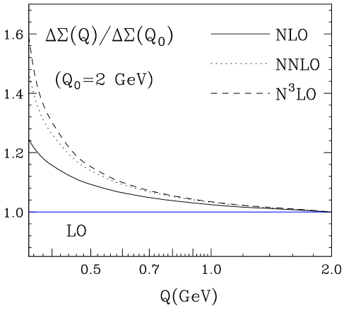
Figure 2: Backward evolution of the first moment of the polarized singlet distributions at LO, NLO, NNLO and N³LO, starting from the initial scale $Q=2$ GeV.

The solution of the evolution equation for the gluon spin contribution now follows directly. From the lower row in Eq. (34) we have by simple integration and using again $d\ln Q^{2}=da_{s}/\beta(a_{s})$

$$\Delta\Gamma(Q^{2}) = \Delta\Gamma(Q_{0}^{2})-\int_{a_{0}}^{a_{Q}}da_{s}\,\frac{\Delta P_{\Sigma\Sigma}(a_{s})}{2N_{f}\beta(a_{s})}\,\Delta\Sigma(Q^{2})$$ (39)

$$= \Delta\Gamma(Q_{0}^{2})+\int_{a_{0}}^{a_{Q}}\frac{da_{s}}{\beta(a_{s})}\,a_{s}\,\Delta P_{Gq}(a_{s})\,\Delta\Sigma(Q^{2})\,,$$

where again $a_{Q}\equiv a_{s}(Q^{2})$ and $a_{0}\equiv a_{s}(Q_{0}^{2})$, and where in the second line we have used Eq. (25) to replace $\Delta P_{\Sigma\Sigma}$ by $\Delta P_{Gq}$, which is more natural in the case of the gluon distribution.

An immediate observation is that the integral on the right-hand-side of (39) starts at order $a_{s}(Q^{2})$ and $a_{s}(Q_{0}^{2})$. Therefore, we arrive at the well-known result [17, 18, 23] that the leading term in $\Delta\Gamma$ is a constant in $Q^{2}$, so that the first moment of the gluon spin contribution evolves as the inverse of the strong coupling. Inserting the solution for $\Delta\Sigma(Q^{2})$ from Eq. (38) into (39) and carrying out the integration, we find the full NNLO analytical solution

$$\Delta G(Q^{2})\,=\,\frac{a_{s}(Q_{0}^{2})}{a_{s}(Q^{2})}\,\Delta G(Q_{0}^{2})\,+\,\Delta\Sigma(Q_{0}^{2})\,F\Big{(}a_{s}(Q^{2}),a_{s}(Q_{0}^{2})\Big{)}\,,$$ (40)

where

$$F(a_{Q},a_{0})\,=\,F^{{\mathrm{LO}}}\left(\frac{a_{0}}{a_{Q}}\right)\,+\,a_{Q}\,F^{{\mathrm{NLO}}}\left(\frac{a_{0}}{a_{Q}}\right)\,+\,a_{Q}^{2}\,F^{{\mathrm{NNLO}}}\left(\frac{a_{0}}{a_{Q}}\right)\,,$$ (41)

with

$$F^{{\mathrm{LO}}}(r) = -(1-r)\frac{\Delta P^{(0)}_{Gq}}{\beta_{0}}\,,$$

$$F^{{\mathrm{NLO}}}(r) = \frac{1-r^{2}}{2\beta_{0}^{2}}\left(\beta_{1}\,\Delta P^{(0)}_{Gq}-\beta_{0}\,\Delta P^{(1)}_{Gq}\right)+\frac{(1-r)^{2}}{2\beta_{0}^{2}}\,\Delta P^{(0)}_{Gq}\,\Delta P_{\Sigma\Sigma}^{(1)}\,,$$

$$F^{{\mathrm{NNLO}}}(r) = \frac{1-r^{3}}{3\beta_{0}^{3}}\left(\beta_{0}\beta_{2}\,\Delta P^{(0)}_{Gq}-\beta_{1}^{2}\,\Delta P^{(0)}_{Gq}+\beta_{0}\beta_{1}\,\Delta P^{(1)}_{Gq}-\beta_{0}^{2}\,\Delta P^{(2)}_{Gq}\right)$$ (42)

$$+ \frac{(1-r)^{2}}{6\beta_{0}^{3}}\left[-\,3(1+r)\beta_{1}\,\Delta P^{(0)}_{Gq}\,\Delta P_{\Sigma\Sigma}^{(1)}+(2+r)\beta_{0}\,\Delta P^{(1)}_{Gq}\,\Delta P_{\Sigma\Sigma}^{(1)}\right.$$

$$\left.\hskip 47.80042pt+\,(1+2r)\,\beta_{0}\,\Delta P^{(0)}_{Gq}\,\Delta P_{\Sigma\Sigma}^{(2)}\right]\,-\,\frac{(1-r)^{3}}{6\beta_{0}^{3}}\,\Delta P^{(0)}_{Gq}\,\big{(}\Delta P_{\Sigma\Sigma}^{(1)}\big{)}^{2}\,.$$

We note that in contrast to $\Delta\Sigma$, we can only give the NNLO evolution of $\Delta G$ here. This is due to the fact that $\Delta\Gamma$ is shifted by one power of $a_{s}$ relative to $\Delta G$. In order to obtain the N³LO solution for $\Delta G$ one would need the four-loop splitting kernel $\Delta P^{(3)}_{Gq}$ which is presently still unavailable.

Figure 3: Evolution of the quark and gluon spin contributions $\frac{1}{2}\Delta\Sigma$ and $\Delta G$ at NNLO, starting from the inital scale $Q=1$ GeV. We also show the evolution of ${\cal L}$ following from Eq. (20).

Figure 3 shows the NNLO evolution of the gluon spin contribution to the proton spin, starting from the values $\Delta G=0.102$ and $\Delta\Sigma=0.254$ at $Q_{0}=1$ as realized in the global analysis [46]. We also show the evolution of $\frac{1}{2}\Delta\Sigma$ and the evolution of the total orbital angular momentum ${\cal L}$ resulting from (20). Notice that both $\Delta G$ and ${\cal L}$ have a divergent behaviour at large scales, resulting in a rather unphysical cancellation of two very large contributions to fulfill the spin sum rule.

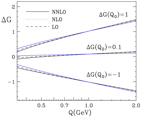
Figure 4: Backward evolution of the gluon spin contribution $\Delta G$ at LO (dashes), NLO (dots) and NNLO (solid line), starting from three different scenarios at the inital scale $Q_{0}=1$ GeV: $\Delta G(Q_{0})=+1,0.1,-1$. The blue solid line corresponds to the leading $1/a_{s}$ term in Eq. (40).

As we discussed above for the singlet contribution, it is also interesting to analyze the behavior of the gluonic spin contribution at lower scales. In Fig. 4 we show the backward evolution of $\Delta G$ at LO (dashes), NLO (dots) and NNLO (solid line) for three different scenarios, corresponding to setting $\Delta G(Q_{0})=+1,0.1,-1$ at the initial scale $Q_{0}=1$ GeV . For each scenario, we observe a striking convergence of the fixed order results down to very low scales, always towards small gluonic contributions. Even though the ”$F$” term in Eq. (40) contains corrections proportional to positive powers of $\alpha_{s}$ that could spoil the convergence of the expansion in the non-perturbative region, the evolution of the gluonic contribution is completely dominated by the leading $1/a_{s}$ term in Eq. (40), as can be observed in Figure 4 where we also present this term separately for each scenario. Our findings set a strong constraint on the proton spin content carried by gluons at hadronic scales. Within the rather extreme scenarios analyzed here (for which the gluon contribution accounts for as much as twice the spin of the proton at $Q_{0}=1$ GeV!), we obtain the requirement $|\Delta G(Q\sim 0.35\,{\rm GeV})|\lesssim 0.3$. Indeed, the few available model estimates of $\Delta G$ suggest values of the order $0.2-0.3$ [41, 42, 43, 44, 45] at a low hadronic scale.

5 “Static” value of $\Delta G$

As we have discussed, $\Delta G(Q^{2})$ in general evolves as $1/a_{s}(Q^{2})$ for large scales. As inspection of Eq. (40) shows, depending on the input values of $\Delta G(Q_{0}^{2})$ and $\Delta\Sigma(Q_{0}^{2})$ the evolution can be towards large positive or negative values. This implies that there is a specific input, a “critical point”, for which $\Delta G(Q^{2})$ actually remains almost constant [26] and tends to a finite asymptotic value as $Q^{2}\rightarrow\infty$. This “static” value of $\Delta G$ is expected to change from order to order in perturbation theory. To determine it at a given order, we only need to tune the input such that the $1/a_{s}(Q^{2})$ term in the solution for $\Delta G(Q^{2})$ is canceled. Starting from Eq. (40) we demand

$$a_{s}(Q_{0}^{2})\,\Delta G(Q_{0}^{2})\,+\,a_{s}(Q^{2})\,\Delta\Sigma(Q_{0}^{2})\,F\Big{(}a_{s}(Q^{2}),a_{s}(Q_{0}^{2})\Big{)}\,=\,{\cal O}\big{(}a_{s}(Q^{2})\big{)}\,.$$ (43)

To LO, using (4), this condition becomes

$$\Delta G_{\mathrm{stat}}^{{\mathrm{LO}}}(Q_{0}^{2})\,=\,-\Delta\Sigma(Q_{0}^{2})\,\frac{\Delta P^{(0)}_{Gq}}{\beta_{0}}=-\frac{4}{9}\,\Delta\Sigma(Q_{0}^{2})\,\simeq\,-0.113\,,$$ (44)

where we have used $N_{f}=3$ flavors and again $\Delta\Sigma(Q_{0}^{2}=1\,{\mathrm{GeV}}^{2})=0.254$. The gluon spin contribution then remains constant at the value $\Delta G_{\mathrm{stat}}^{{\mathrm{LO}}}(Q_{0}^{2})$.

At NLO, the necessary input value for the static solution becomes

$$\Delta G_{\mathrm{stat}}^{{\mathrm{NLO}}}(Q_{0}^{2}) = -\Delta\Sigma(Q_{0}^{2})\left[\,\frac{\Delta P^{(0)}_{Gq}}{\beta_{0}}+a_{0}\frac{-\beta_{1}\,\Delta P^{(0)}_{Gq}+\beta_{0}\,\Delta P^{(1)}_{Gq}+\Delta P^{(0)}_{Gq}\,\Delta P_{\Sigma\Sigma}^{(1)}}{2\beta_{0}^{2}}\,\right]$$ (45)

$$= -\left[\,\frac{4}{9}+\frac{166}{81}\,a_{0}\,\right]\Delta\Sigma(Q_{0}^{2})\,\simeq\,-0.13\,.$$

The NLO “static” solution is no longer completely constant in $Q^{2}$. However, by construction it does converge asymptotically to a finite value, given by

$$\Delta G_{\mathrm{stat}}^{{\mathrm{NLO}}}(\infty) = -\Delta\Sigma(Q_{0}^{2})\left[\,\frac{\Delta P^{(0)}_{Gq}}{\beta_{0}}+a_{0}\,\frac{\Delta P^{(0)}_{Gq}\,\Delta P_{\Sigma\Sigma}^{(1)}}{\beta_{0}^{2}}\right]$$ (46)

$$= -\left[\,\frac{4}{9}-\frac{32}{27}\,a_{0}\,\right]\Delta\Sigma(Q_{0}^{2})\,\simeq\,-0.103\,.$$

We note that a value of similar size was in fact found in the early NLO DSSV analysis [25, 26, 27].

Finally, at NNLO, the corresponding values are

$$\Delta G_{\mathrm{stat}}^{{\mathrm{NNLO}}}(Q_{0}^{2}) = -\Delta\Sigma(Q_{0}^{2})\Bigg{[}\,\frac{\Delta P^{(0)}_{Gq}}{\beta_{0}}+a_{0}\,\frac{-\beta_{1}\,\Delta P^{(0)}_{Gq}+\beta_{0}\,\Delta P^{(1)}_{Gq}+\Delta P^{(0)}_{Gq}\,\Delta P_{\Sigma\Sigma}^{(1)}}{2\beta_{0}^{2}}$$ (47)

$$+ \frac{a_{0}^{2}}{6\beta_{0}^{3}}\Bigg{(}2\beta_{1}^{2}\,\Delta P^{(0)}_{Gq}-2\beta_{0}\,\beta_{2}\,\Delta P^{(0)}_{Gq}-2\beta_{0}\,\beta_{1}\,\Delta P^{(1)}_{Gq}+2\beta_{0}^{2}\,\Delta P^{(2)}_{Gq}$$

$$+ 2\beta_{0}\,\Delta P^{(0)}_{Gq}\,\Delta P_{\Sigma\Sigma}^{(2)}-3\beta_{1}\,\Delta P^{(0)}_{Gq}\,\Delta P_{\Sigma\Sigma}^{(1)}+\beta_{0}\,\Delta P^{(1)}_{Gq}\,\Delta P_{\Sigma\Sigma}^{(1)}+\Delta P^{(0)}_{Gq}\,\big{(}\Delta P_{\Sigma\Sigma}^{(1)}\big{)}^{2}\Bigg{)}\,\Bigg{]}$$

$$= -\left[\,\frac{4}{9}+\frac{166}{81}a_{0}-\left(\,\frac{7561}{2187}-\frac{160}{9}\zeta_{3}\right)a_{0}^{2}\,\right]\Delta\Sigma(Q_{0}^{2})\,\simeq\,-0.125\,,$$

with an asymptotic value given by

$$\Delta G_{\mathrm{stat}}^{{\mathrm{NNLO}}}(\infty) = -\Delta\Sigma(Q_{0}^{2})\left[\,\frac{\Delta P^{(0)}_{Gq}}{\beta_{0}}+a_{0}\frac{\Delta P^{(0)}_{Gq}\,\Delta P_{\Sigma\Sigma}^{(1)}}{\beta_{0}^{2}}\right.$$ (48)

$$\left.\hskip 61.17325pt+\,a_{0}^{2}\,\Delta P^{(0)}_{Gq}\;\frac{-\beta_{1}\,\Delta P_{\Sigma\Sigma}^{(1)}+\big{(}\Delta P_{\Sigma\Sigma}^{(1)}\big{)}^{2}+\beta_{0}\,\Delta P_{\Sigma\Sigma}^{(2)}}{2\beta_{0}^{3}}\,\right]$$

$$= -\left[\,\frac{4}{9}-\frac{32}{27}\,a_{0}-\frac{1328}{243}\,a_{0}^{2}\right]\Delta\Sigma(Q_{0}^{2})\,\simeq\,-0.102\,.$$

Numerical results for the “static” solutions for $\Delta G$ are shown in Fig. 5.

Figure 5: Evolution of the ”static” gluon solutions, starting from the inital scale $Q_{0}=1$ GeV.

At NNLO the sum of the contributions by quarks and gluons starts at $\Delta\Sigma(Q_{0}^{2})/2+G_{\mathrm{stat}}^{{\mathrm{NNLO}}}(Q_{0}^{2})=0.0025$ with an asymptotic result of $\Delta\Sigma(\infty)/2+G_{\mathrm{stat}}^{{\mathrm{NNLO}}}(\infty)=0.01335$. In that particular scenario the total orbital angular momentum almost accounts for the entire proton spin, $L_{q}+L_{g}\simeq 1/2$, and is almost constant in $Q^{2}$ (from $Q_{0}^{2}=1$ to $\infty$ it varies by less than 3%).

As mentioned above, in our study of the “static” $\Delta G$ we have for simplicity chosen a fixed number of flavors, $N_{f}=3$. This will not be entirely adequate when considering the limit of large $Q^{2}$, and a matching to $N_{f}=4$ and $N_{f}=5$ should be performed at the charm and bottom mass scales, respectively. For the inputs $\Delta G_{\mathrm{stat}}(Q_{0}^{2})$ given explicitly above, each matching would slightly upset the cancelation of the $1/a_{s}$ term in the solution for $\Delta G$, so that the resulting gluon spin contribution would not be entirely “static” anymore. However, this is expected to be a small effect. We have checked that using a fixed number of $N_{f}$ throughout changes the asymptotic value of the static $\Delta G$ by less than $10\%$. In any case, it is clear that a static solution for $\Delta G$ exists even if one performs a full matching to $N_{f}=4$ and $N_{f}=5$: One could always start with an input at the bottom mass, $Q_{0}^{2}=m_{b}^{2}$, that creates a static solution for all higher $Q^{2}$ with $N_{f}=5$. This solution could then be evolved backward to any lower $Q^{2}$ one desires, even to $Q^{2}=1~{}{\mathrm{GeV}}^{2}$ where $N_{f}=3$. This result at $Q^{2}=1~{}{\mathrm{GeV}}^{2}$ would then be the input to be used to obtain a static solution with full matching.

We believe these solutions, especially because of the fact that they have a well behaved asymptotic limit at large scales, deserve further attention since they arise as strong boundaries on non-perturbative physics from almost purely perturbative considerations.

6 Non-singlet evolution of the valence quark spin contribution

We finally turn to the evolution in the non-singlet sector. As discussed in the Introduction, we focus here on the strangeness “valence” spin contribution $(\Delta s-\Delta\bar{s})(Q^{2})$ generated by three-loop evolution.

Each of the non-singlet evolution equations in Eq. (10) has the solution

$$\Delta q^{(A)}(Q^{2})=U^{(A)}(Q,Q_{0})\;\Delta q^{(A)}(Q_{0}^{2})\;\;,\quad(A=V,\pm)\;,$$ (49)

where $\Delta q^{(A)}(Q_{0}^{2})$ is the corresponding input non-singlet combination and the evolution operator $U^{(A)}$ is given by

$$U^{(A)}(Q,Q_{0})\,=\,\exp\left\{\int_{Q_{0}^{2}}^{Q^{2}}\frac{dq^{2}}{q^{2}}\;\Delta P^{(A)}(a_{s}(q^{2}))\right\}\;\;.$$ (50)

We may readily use (49) with $A=-$ and $A=V$ to obtain the solution for a valence quark contribution $\Delta q-\Delta{\bar{q}}$, resulting in [33]

$$\left(\Delta q-\Delta{\bar{q}}\right)(Q^{2})\,=\,U^{(-)}(Q,Q_{0})\left[\,\left(\Delta q-\Delta{\bar{q}}\right)(Q_{0}^{2})+\frac{1}{N_{f}}\left(\frac{U^{(V)}(Q,Q_{0})}{U^{(-)}(Q,Q_{0})}-1\right)\Delta q^{(V)}(Q_{0}^{2})\right]\;,$$ (51)

where $\Delta q^{(V)}(Q_{0}^{2})=\sum_{q}\left(\Delta q-\Delta\bar{q}\,\right)(Q_{0}^{2})$ is the total spin-dependent valence distribution in the nucleon as defined in Eq. (9), at the initial scale. The first term on the right represents the homogenous component of the evolution of the valence distribution, which starts at NLO; its explicit expression is identical to the one in Eq. (38) with the change $\Delta P_{\Sigma\Sigma}\rightarrow\Delta P^{(-)}$. As follows from Eq. (11), $\Delta P^{(V)}-\Delta P^{(-)}=N_{f}\left(\Delta P_{qq}^{S}-\Delta P_{q\bar{q}}^{S}\right)$, which (see Eqs. (3)–(3)) becomes nonzero starting from NNLO. Therefore, the second term on the right of (51) will in general be non-vanishing as well, as long as $\Delta q^{(V)}(Q_{0}^{2})\neq 0$, which of course is the case. We conclude that NNLO evolution generates an asymmetry $\Delta s\neq\Delta\bar{s}$ in the contribution by strange and anti-strange quarks to the proton spin, even if $\Delta s=\Delta\bar{s}$ at the initial scale $Q_{0}$. This is at variance with the spin-averaged case where the first moment of $s-\bar{s}$ is protected by the fact that there can be no net valence strangeness in the proton and remains zero to all orders.

To NNLO accuracy, the evolution factor in the second term in Eq.(51) reduces to

$$\frac{U^{(V)}(Q,Q_{0})}{U^{(-)}(Q,Q_{0})}-1\,=\,-\frac{N_{f}\left(\Delta P^{(2)S}_{qq}-\Delta P^{(2)S}_{q\bar{q}}\,\right)}{2\beta_{0}}\,\left(a_{Q}^{2}-a_{0}^{2}\right)\;,$$ (52)

where, as before $a_{Q}=a_{s}(Q^{2})$ and $a_{0}=a_{s}(Q_{0}^{2})$. Therefore, assuming $\Delta s(Q_{0}^{2})=\Delta\bar{s}(Q_{0}^{2})$ in order to estimate the purely perturbative effect, we have, to NNLO

$$\left(\Delta s-\Delta{\bar{s}}\right)_{\mathrm{pert}}(Q^{2})\,=\,-\frac{\Delta P^{(2)S}_{qq}-\Delta P^{(2)S}_{q\bar{q}}}{2\beta_{0}}\,\left(a_{Q}^{2}-a_{0}^{2}\right)\left(\Delta u-\Delta\bar{u}+\Delta d-\Delta\bar{d}\,\right)(Q_{0}^{2})$$

$$\hskip 12.80373pt\,=\,-\frac{5(23-12\zeta_{2}-16\zeta_{3})}{72\beta_{0}\pi^{2}}\left(\alpha_{s}(Q^{2})-\alpha_{s}(Q_{0}^{2})\right)\left(\Delta u-\Delta\bar{u}+\Delta d-\Delta\bar{d}\,\right)(Q_{0}^{2}),$$ (53)

where in the second line we have inserted the explicit value of $\left(\Delta P^{(2)S}_{qq}-\Delta P^{(2)S}_{q\bar{q}}\,\right)$ from Eq. (3). The last factor on the right is of course just the total valence spin contribution at the initial scale.

We estimate the polarized strange asymmetry generated perturbatively by assuming, for example, $Q_{0}=1$ GeV with $\alpha_{s}(Q_{0}^{2})=0.404$, and [26, 27, 46] $\left(\Delta u-\Delta\bar{u}+\Delta d-\Delta\bar{d}\,\right)(Q_{0}^{2})\sim 0.5$, for which

$$\left(\Delta s-\Delta{\bar{s}}\right)_{\mathrm{pert}}(Q^{2}=10\,{\mathrm{GeV}}^{2})\,\approx\,-6\,\cdot\,10^{-4}\,.$$ (54)

Figure 6: Evolution of the perturbatively generated “valence” strange contribution $\Delta s_{\mathrm{V}}\equiv\Delta s-\Delta{\bar{s}}$, starting from the inital scale $Q_{0}=1$ GeV.

Figure 6 shows $\Delta s_{\mathrm{V}}\equiv\Delta s-\Delta{\bar{s}}$ as a function of $Q$. The difference reaches $-0.001$ at $Q=M_{Z}$. As expected for a three-loop effect, it is small. On the other hand, for the latest extractions of $(\Delta s+\Delta\bar{s})$ [47] the relative asymmetry $|\Delta s-\Delta\bar{s}|/|\Delta s+\Delta\bar{s}|$ would be of order $1\%$. Evidently, non-perturbative contributions [34] may well be the dominant source of the polarized strangeness asymmetry. However, the effect we describe here would certainly need to be taken into account in a full analysis. We emphasize that the perturbative asymmetry is robustly predicted to be negative, so that $\Delta\bar{s}>\Delta s$.

7 Conclusions

We have presented a set of studies of the evolution of the quark and gluon spin contributions to the proton spin at higher orders in perturbation theory, motivated by the recent calculations of the helicity splitting functions at full NNLO [10, 11, 12]. We have argued that the evolution of $\Delta\Sigma$ is known even to four loops, which may prove valuable for lattice studies, as well as for comparisons to models residing at lower “hadronic” scales. The anomalous dimension relevant for the evolution of $\Delta\Sigma$ and related to the axial anomaly also turns out to generate the evolution of $\Delta G$. The same must then be true for the total orbital angular momentum $L_{q}+L_{g}$ in the Jaffe-Manohar sum rule, although the separate evolutions of $L_{q}$ and $L_{g}$ are presently only known to LO.

We have obtained analytical higher-order solutions for $\Delta\Sigma$ and $\Delta G$ and presented numerical results for their evolution. These show a stable upturn of $\Delta\Sigma$ toward low scales, bringing it actually closer to quark model expectations that favor a large quark spin contribution to the proton spin. The gluon spin $\Delta G$, when evolved backwards, shows a remarkable focus towards low values, again in line with quark model assumptions, setting a strong constraint on the gluon contribution at hadronic scales. We have also shown that at every order of the perturbative evolution, there is a unique solution for which $\Delta G$ tends to a finite asymptotic value as the scale becomes large. We have estimated the values of $\Delta G$ in such a scenario.

We have finally also examined the size of the new effect arising from three-loop evolution in the flavor non-singlet sector, the generation of an asymmetry in the strange and anti-strange contributions to the proton spin. We have found that perturbative evolution predicts $\Delta s-\Delta{\bar{s}}$ to be negative, with a magnitude of order $1\%$ of the total $\Delta s+\Delta{\bar{s}}$.

References

• [1] R. L. Jaffe and A. Manohar, Nucl. Phys. B 337, 509 (1990).
• [2] X. D. Ji, Phys. Rev. Lett.  78, 610 (1997) [hep-ph/9603249].
• [3] For review, see: E. Leader and C. Lorcé, Phys. Rept.  541, no. 3, 163 (2014) [arXiv:1309.4235 [hep-ph]].
• [4] M. A. Ahmed and G. G. Ross, Nucl. Phys. B 111, 441 (1976).
• [5] G. Altarelli and G. Parisi, Nucl. Phys. B 126 (1977) 298.
• [6] J. Kodaira, Nucl. Phys. B 165, 129 (1980).
• [7] R. Mertig and W. L. van Neerven, Z. Phys. C 70 (1996) 637 [hep-ph/9506451].
• [8] W. Vogelsang, Phys. Rev. D 54 (1996) 2023 [hep-ph/9512218].
• [9] W. Vogelsang, Nucl. Phys. B 475 (1996) 47 [hep-ph/9603366].
• [10] A. Vogt, S. Moch, M. Rogal and J. A. M. Vermaseren, Nucl. Phys. Proc. Suppl.  183, 155 (2008) [arXiv:0807.1238 [hep-ph]].
• [11] S. Moch, J. A. M. Vermaseren and A. Vogt, Nucl. Phys. B 889 (2014) 351 [arXiv:1409.5131 [hep-ph]].
• [12] S. Moch, J. A. M. Vermaseren and A. Vogt, Phys. Lett. B 748 (2015) 432 [arXiv:1506.04517 [hep-ph]].
• [13] X. D. Ji, J. Tang and P. Hoodbhoy, Phys. Rev. Lett.  76, 740 (1996) [hep-ph/9510304].
• [14] P. Hägler and A. Schäfer, Phys. Lett. B 430, 179 (1998) [hep-ph/9802362].
• [15] A. Harindranath and R. Kundu, Phys. Rev. D 59, 116013 (1999) [hep-ph/9802406].
• [16] G. Altarelli and B. Lampe, Z. Phys. C 47, 315 (1990).
• [17] P. G. Ratcliffe, Phys. Lett. B 192, 180 (1987).
• [18] G. P. Ramsey, J. W. Qiu, D. Richards and D. W. Sivers, Phys. Rev. D 39, 361 (1989).
• [19] M. Stratmann and W. Vogelsang, J. Phys. Conf. Ser.  69, 012035 (2007) [hep-ph/0702083].
• [20] A. W. Thomas, Phys. Rev. Lett.  101, 102003 (2008) [arXiv:0803.2775 [hep-ph]].
• [21] M. Altenbuchinger, P. Hägler, W. Weise and E. M. Henley, Eur. Phys. J. A 47, 140 (2011) [arXiv:1012.4409 [hep-ph]].
• [22] For review, see: H. W. Lin et al., Prog. Part. Nucl. Phys.  100, 107 (2018) [arXiv:1711.07916 [hep-ph]].
• [23] G. Altarelli and G. G. Ross, Phys. Lett. B 212, 391 (1988).
• [24] G. Altarelli and W. J. Stirling, Part. World 1, no. 2, 40 (1989).
• [25] W. Vogelsang, talk presented at the workshop RHIC Spin: Next Decade, Lawrence Berkeley National Laboratory, Nov. 20-22, 2009.
• [26] D. de Florian, R. Sassot, M. Stratmann and W. Vogelsang, Phys. Rev. D 80, 034030 (2009) [arXiv:0904.3821 [hep-ph]].
• [27] D. de Florian, R. Sassot, M. Stratmann and W. Vogelsang, Phys. Rev. Lett.  101 (2008) 072001 [arXiv:0804.0422 [hep-ph]].
• [28] D. A. Ross and C. T. Sachrajda, Nucl. Phys. B 149 (1979) 497.
• [29] W. Furmanski and R. Petronzio, Z. Phys. C 11 (1982) 293.
• [30] M. Stratmann, A. Weber and W. Vogelsang, Phys. Rev. D 53, 138 (1996) [hep-ph/9509236].
• [31] S. Moch, J. A. M. Vermaseren and A. Vogt, Nucl. Phys. B 688, 101 (2004) [hep-ph/0403192].
• [32] S. Catani and F. Hautmann, Nucl. Phys. B 427 (1994) 475 [arXiv:hep-ph/9405388].
• [33] S. Catani, D. de Florian, G. Rodrigo and W. Vogelsang, Phys. Rev. Lett.  93 (2004) 152003 [hep-ph/0404240].
• [34] X. G. Wang, C. R. Ji, W. Melnitchouk, Y. Salamu, A. W. Thomas and P. Wang, Phys. Rev. D 94, no. 9, 094035 (2016) [arXiv:1610.03333 [hep-ph]].
• [35] S. A. Larin, T. van Ritbergen and J. A. M. Vermaseren, Nucl. Phys. B 427, 41 (1994).
• [36] S. A. Larin, P. Nogueira, T. van Ritbergen and J. A. M. Vermaseren, Nucl. Phys. B 492, 338 (1997) [hep-ph/9605317].
• [37] J. Kodaira, S. Matsuda, K. Sasaki and T. Uematsu, Nucl. Phys. B 159, 99 (1979); J. Kodaira, S. Matsuda, T. Muta, K. Sasaki and T. Uematsu, Phys. Rev. D 20, 627 (1979).
• [38] J. D. Bjorken, Phys. Rev.  148, 1467 (1966).
• [39] S. A. Larin, Phys. Lett. B 303 (1993) 113 [hep-ph/9302240].
• [40] R. L. Jaffe, Phys. Lett. B 193, 101 (1987).
• [41] R. L. Jaffe, Phys. Lett. B 365, 359 (1996) [hep-ph/9509279].
• [42] V. Barone, T. Calarco and A. Drago, Phys. Lett. B 431, 405 (1998) [hep-ph/9801281].
• [43] H. J. Lee, D. P. Min, B. Y. Park, M. Rho and V. Vento, Phys. Lett. B 491, 257 (2000) [hep-ph/0006004].
• [44] P. Chen and X. Ji, Phys. Lett. B 660, 193 (2008) [hep-ph/0612174].
• [45] S. D. Bass, A. Casey and A. W. Thomas, Phys. Rev. C 83, 038202 (2011) [arXiv:1110.5160 [hep-ph]].
• [46] D. de Florian, R. Sassot, M. Stratmann and W. Vogelsang, Phys. Rev. Lett.  113 (2014) no.1, 012001 [arXiv:1404.4293 [hep-ph]].
• [47] J. J. Ethier, N. Sato and W. Melnitchouk, Phys. Rev. Lett.  119, no. 13, 132001 (2017) [arXiv:1705.05889 [hep-ph]].