Derivative-based global sensitivity analysis for models with high-dimensional inputs and functional outputs

Abstract

We present a framework for derivative-based global sensitivity analysis (GSA) for models with high-dimensional input parameters and functional outputs. We combine ideas from derivative-based GSA, random field representation via Karhunen–Loève expansions, and adjoint-based gradient computation to provide a scalable computational framework for computing the proposed derivative-based GSA measures. We illustrate the strategy for a nonlinear ODE model of cholera epidemics and for elliptic PDEs with application examples from geosciences and biotransport.

65C20, 65C50, 62H99, 65D15.

1 Introduction

The field of global sensitivity analysis (GSA) provides methods for quantifying how the uncertainty in the output of mathematical models can be apportioned to uncertainties in the input model parameters [37]. Specifically, variance-based GSA enables ranking the importance of model parameters by computing their relative contribution to the variance of the output quantities of interest (QoIs), as quantified by Sobol’ indices [41, 37, 42]. Another popular GSA approach involves using derivative-based global sensitivity measures (DGSMs) [43, 23], which have been shown to provide efficient means of screening for unimportant input parameters. In this article, we consider mathematical models of the form

(1) $$y=f(s,\theta),$$

where $s$ belongs to a compact set $\mathscr{X}\subset\mathbb{R}^{d}$ with $d=1,2$, or $3$, and $\theta$ is an element of an uncertain parameter space $\Theta\subseteq\mathbb{R}^{N_{\text{par}}}$. We present a mathematical framework for derivative-based GSA for functional QoIs of the form Eq. 1 and present a scalable computational framework for computing the corresponding derivative-based GSA measures.

Survey of literature and existing approaches. A great amount of progress has been made in theory and numerical methods for variance-based GSA over the past three decades [41, 37, 42, 44, 45, 14, 43, 17, 23, 35, 32, 18]. The majority of works on GSA focus on scalar-valued QoIs. However, in recent years there have been a number of efforts targeting GSA for vectorial or functional QoIs. Specifically, the works [8, 26, 17, 47, 4] discuss variance-based GSA for vectorial and functional outputs. Computing GSA measures for functional QoIs, as is the case for their scalar counterparts, is computationally challenging. The computational challenges can be reduced significantly by employing surrogate models [45, 14, 3, 39, 19, 4]. However, surrogate model construction itself becomes computationally challenging for models with high-dimensional input parameters.

DGSMs have been shown to provide efficient means for detecting unimportant input parameters [24, 23, 46]. For a scalar QoI $g(\theta)$ that has square integrable partial derivatives, the DGSMs, defined as $\mathrm{E}\big{\{}(\frac{\partial g}{\partial\theta_{j}})^{2}\big{\}}$, $j=1,\ldots,{N_{\text{par}}}$, are commonly used. (Here $\mathrm{E}$ denotes expectation with respect to $\theta$.) These DGSMs can be used to bound the total Sobol’ indices, for models with statistically independent inputs, which justifies their use in screening for unimportant inputs.

An alternate approach for approximating the DGSMs, for scalar-valued QoIs, using the active subspace method [13, 11] is presented in [12]. Namely, [12] presents a method for approximating the DGSMs using dominant eigenpairs of the matrix $\mathrm{E}\left\{{\nabla f(\theta)\nabla f(\theta)^{\top}}\right\}$. While active subspace methods have mostly targeted scalar QoIs, recently there have been initial efforts in generalizing these methods to vectorial outputs; see e.g., [22, 49].

Our approach and contributions. We focus on functional QoIs of the form $f:\mathscr{X}\times\Theta\to\mathbb{R}$, as defined in Eq. 1, where $\mathscr{X}$ and $\Theta$ are as before. We focus on models with independent random input parameters. Moreover, in our target applications, $f(s,\theta)$ is defined in terms of the solution of a system of differential equations.

We begin our developments by defining a suitable DGSM for functional QoIs, in Section 3, and prove that it provides a computable bound for the generalized total Sobol’ indices for functional QoIs as defined in [17, 4]; see Theorem 3.3. Next, we present a framework for efficient computation of the functional DGSMs that uses low-rank representation of the functional QoIs via truncated Karhunen–Loève (KL) expansions [28]. Expressions for DGSMs, and DGSM-based bounds on functional total Sobol’ indices for a truncated KL expansion are established in Theorem 3.7. The DGSMs of the approximate models, given by truncated KL expansions, are then computed using adjoint-based gradient computation. This approach is elaborated for models governed by linear elliptic PDEs in Section 4.

Additionally, we present a comprehensive set of numerical results that illustrate various aspects of the proposed approach and demonstrate its effectiveness. We consider three application problems: (i) a nonlinear system of ODEs modeling the spread of cholera [20], where we perform GSA for the infected population as a function of time (Section 5.1); (ii) a problem motivated by porous medium flow applications, with permeability data adapted from [1], where we assess parametric sensitivities of the pressure field on a domain boundary (Section 5.2); and (iii) an application problem involving biotransport in tumors [6], where we consider the pressure distribution in certain subdomains of a tumor model (Section 5.3).

Article overview. This article is structured as follows. In Section 2, we set up the notation used throughout the article, and collect the assumptions on the functional QoIs under study. We also provide a brief review of variance-based GSA for functional QoIs, following the developments in [17, 4], in Section 2. In Section 3 we present a mathematical framework for derivative-based GSA of functional QoIs. We elaborate our proposed adjoint-based framework for models governed by linear elliptic PDEs in Section 4. This is followed by our computational experiments that are detailed in Section 5. Finally, we provide some concluding remarks in Section 6.

2 Preliminaries

2.1 The basic setup

Let $\Theta\subseteq\mathbb{R}^{N_{\text{par}}}$ be the uncertain parameter space, and consider the probability space $(\Theta,\mathcal{B},\mu)$, where $\mathcal{B}$ is the Borel $\sigma$-algebra on $\Theta$ and $\mu$ is the law of the uncertain parameter vector $\theta$. In the present work, $\Theta$ is of the form $\Theta=\Theta_{1}\times\Theta_{2}\times\cdots\times\Theta_{N_{\text{par}}}$, where $\Theta_{j}\subseteq\mathbb{R}$, $j=1,\ldots,{N_{\text{par}}}$. The expectation of a random variable $g:\Theta\to\mathbb{R}$ is denoted by

$$\mathrm{E}\left\{{g}\right\}=\int_{\Theta}g(\theta)\mu(d\theta).$$

We assume the components of the random vector $\theta$ are independent and admit probability density functions $\pi_{j}(\theta_{j})$, in which case $\mu(d\theta)=\prod_{j=1}^{N_{\text{par}}}\pi_{j}(\theta_{j})d\theta_{j}$. Next, let $\mathscr{X}\subset\mathbb{R}^{d}$, with $d=1,2$, or $3$ be a compact set. With this setup, we consider a process, $f:\mathscr{X}\times\Theta\to\mathbb{R}$ as in Eq. 1. Note that this setup covers both time-dependent and spatially distributed processes. In the former case, $\mathscr{X}$ is a time interval, and in the latter case, $\mathscr{X}$ is a spatial region.

Assumptions on the process. We consider random processes that satisfy the following assumptions.

Assumption 2.1.

We assume

1. $f\in L^{2}(\mathscr{X}\times\Theta)$ and $f$ is mean square continuous; that is, for any sequence $\{s_{n}\}$ in $\mathscr{X}$ converging to $s\in\mathscr{X}$ we have that $\lim_{n\rightarrow\infty}\mathrm{E}\left\{{[f(s_{n},\theta)-f(s,\theta)]^{2}}\right\}=0$.

2. $\frac{\partial f}{\partial\theta_{j}}(s,\theta)$is defined for all $s\in\mathscr{X}$ and $\theta\in\Theta$, $j=1,\ldots,{N_{\text{par}}}$;

3. $\frac{\partial f}{\partial\theta_{j}}(s,\theta)\in L^{2}(\mathscr{X}\times\Theta)$, $j=1,\ldots,{N_{\text{par}}}$;

4. and $\{\theta_{j}\}_{j=1}^{N_{\text{par}}}$, are real-valued independent random variables, and have distribution laws that are absolutely continuous with respect to the Lebesgue measure.

We remark that (a) is a fundamental assumption on the process $f$. From this, we can conclude continuity of the mean and covariance function of the process; see, e.g., [21, Theorem 7.3.2], [2, Theorem 2.2.1]. This in turn facilitates application of Mercer’s Theorem [34, 27] (needed below) and implies that $f$ admits a KL expansion [29]. The assumptions (b) and (c) are needed in the context of derivative-based global sensitivity analysis. Note that 2.1(b) can be relaxed by requiring $\frac{\partial f}{\partial\theta_{j}}(s,\theta)$ be defined almost everywhere in $\mathscr{X}\times\Theta$.

2.2 Variance-based sensitivity analysis for functional outputs

We first recall the classical Sobol’ indices and Analysis of Variance (ANOVA) decomposition [44, 42, 41], which can be defined pointwise in $\mathscr{X}$. Let $K=\{1,2,\ldots,{N_{\text{par}}}\}$ be an index set, let $U=\{j_{1},j_{2},\ldots,j_{m}\}$ be a subset of $K$, and let $U^{c}$ be the complement of $U$ in $K$, $U^{c}=K\setminus U$. We denote $\theta_{U}=\{\theta_{j_{1}},\theta_{j_{2}},\ldots,\theta_{j_{m}}\}$. For each $s\in\mathscr{X}$, we have the ANOVA decomposition [44]

(2) $$f(s,\theta)=f_{0}(s)+f_{1}(s,\theta_{U})+f_{2}(s,\theta_{U^{c}})+f_{12}(s,\theta),$$

where $f_{0}$ is the mean of the process, and

$$f_{1}(s,\theta_{U})=\mathrm{E}\left\{{f(s,\cdot)|\theta_{U}}\right\}-f_{0}(s),\quad f_{2}(s,\theta_{U^{c}})=\mathrm{E}\left\{{f(s,\cdot)|\theta_{U^{c}}}\right\}-f_{0}(s),$$

and $f_{12}(s,\theta)=f(s,\theta)-f_{0}(s)-f_{1}(s,\theta_{U})-f_{2}(s,\theta_{U^{c}})$. This enables decomposing the total variance $D(f;s)=\mathrm{Var}\left\{{f(s,\cdot)}\right\}$ of $f(s,\cdot)$ according to

$$D(f;s)=D_{U}(f;s)+D_{U^{c}}(f;s)+D_{U,U^{c}}(f;s),$$

where $D_{U}(f;s)=\mathrm{E}_{{\theta_{U}}}\left\{{f_{1}(s,\theta_{U})^{2}}\right\}$, $D_{U^{c}}(f;s)=\mathrm{E}_{{\theta_{U^{c}}}}\left\{{f_{2}(s,\theta_{U^{c}})^{2}}\right\}$, and $D_{U,U^{c}}(f;s)$ is the remainder. (Here $\mathrm{E}_{{\theta_{U}}}\left\{{\cdot}\right\}$ indicates expectation with respect to $\theta_{U}$.) Then, we can define the first and total order Sobol’ indices as follows:

$$S_{U}(f;s)=\frac{D_{U}(f;s)}{D(f;s)}\quad\text{and}\quad\quad S_{U}^{\text{tot}}(f;s)=\frac{D_{U}^{tot}(f;s)}{D(f;s)},$$

where $D_{U}^{tot}(f;s)=D_{U}(f;s)+D_{U,U^{c}}(f;s)$. Note that,

$$S_{U}^{\text{tot}}(f;s)=\frac{D(f;s)-D_{U^{c}}(f;s)}{D(f;s)}=1-\frac{D_{U^{c}}(f;s)}{D(f;s)}=1-S_{U^{c}}(f;s).$$

When the index set $U$ is a singleton, $U=\{j\}$, $j\in\{1,\ldots,{N_{\text{par}}}\}$, we denote the corresponding first and total order Sobol’ indices by $S_{j}(f;s)$ and $S_{j}^{\text{tot}}(f;s)$, respectively.

Here we assume that $D(f;s)>0$ almost everywhere in $\mathscr{X}$. If $D(f;s)=0$ for some $s\in\mathscr{X}$, we use the convention $S_{U}(f;s)=0$.

2.3 Functional Sobol’ indices

Following [4], we define the functional first order Sobol’ index as

$$\mathfrak{S}_{U}(f;\mathscr{X})=\frac{\int_{\mathscr{X}}D_{U}(f;s)\,ds}{\int_{\mathscr{X}}D(f;s)\,ds}.$$

The following lemma provides a simple representation for the functional Sobol’ index in terms of the pointwise classical Sobol’ indices:

Lemma 2.1.

We have $\mathfrak{S}_{U}(f;\mathscr{X})=\int_{\mathscr{X}}S_{U}(f;s)w(s)\,ds$, with $w(s)=\dfrac{D(f;s)}{\int_{\mathscr{X}}D(f;y)\,dy}$.

Proof 2.2.

The result follows by a straightforward calculation.

We can also define the functional total Sobol’ indices

$$\mathfrak{S}^{\text{tot}}_{U}(f;\mathscr{X})=\frac{\int_{\mathscr{X}}D_{U}^{\text{tot}}(f;s)\,ds}{\int_{\mathscr{X}}D(f;s)\,ds}=1-\mathfrak{S}_{U^{c}}(f;\mathscr{X}).$$

Using Lemma 2.1, we note

(3) $$\mathfrak{S}^{\text{tot}}_{U}(f;\mathscr{X})=1-\mathfrak{S}_{U^{c}}(f;\mathscr{X})=\int_{\mathscr{X}}(1-S_{U^{c}}(f;s))w(s)\,ds=\int_{\mathscr{X}}S_{U}^{\text{tot}}(f;s)w(s)ds.$$

Error estimates. We can use the total Sobol’ index of a parameter to rank its importance. In particular, parameters with small Sobol’ indices can be deemed unimportant. In this section, we briefly discuss the impact of fixing these unimportant parameters in terms of approximation errors. Let $U=\{j_{1},j_{2},\ldots,j_{m}\}\subset\{1,\ldots,{N_{\text{par}}}\}$ index the set of important parameters, and suppose we set $\theta_{U^{c}}$ to a nominal vector $\eta$. Consider the “reduced” model:

$$f^{(\eta)}(s,\theta_{U})=f(s,\theta_{U},\eta),$$

where the right hand side function is understood to be $f(s,\theta)$, with entries of $\theta_{U^{c}}$ fixed at $\eta$.

For $U=\{j_{1},j_{2},\ldots,j_{m}\}$ we define ${\Theta_{U}}=\Theta_{j_{1}}\times\cdots\times\Theta_{j_{m}}$. Integration on ${\Theta_{U}}$ will be with respect to $\mu(d\theta_{U})=\prod_{k=1}^{m}\pi_{j_{k}}(\theta_{j_{k}})d\theta_{j_{k}}$.

For $\eta\in{\Theta_{U^{c}}}$ we define the mean-square error

$$\varepsilon\left({f};s;{\eta}\right)=\int_{\Theta}(f(s,\theta)-f^{(\eta)}(s,\theta_{U}))^{2}\,\mu(d\theta).$$

We consider the relative mean square error

(4) $$\mathcal{E}(f;\eta)=\frac{\displaystyle\int_{\mathscr{X}}\int_{\Theta}(f(s,\theta)-f^{(\eta)}(s,\theta_{U}))^{2}\,\mu(d\theta)ds}{\displaystyle\int_{\mathscr{X}}\int_{\Theta}f(s,\theta)^{2}\,\mu(d\theta)ds}.$$

This provides a measure of the error that occurs when fixing the values of $\theta_{U^{c}}$. The following proposition quantifies this error in terms of the functional total Sobol’ indices. This result is a straightforward modification of the error estimate presented in [4]; we provide a proof in Appendix A for completeness.

Proposition 2.3.

$\int_{\Theta_{U^{c}}}\mathcal{E}(f;\eta)\mu(d\eta)\leq 2\mathfrak{S}^{\text{tot}}_{\theta_{U^{c}}}(f,\mathscr{X})$.

Proof 2.4.

See Appendix A.

The estimate in Proposition 2.3 says that when fixing $\theta_{U^{c}}$ to a nominal parameter $\eta\in{\Theta_{U^{c}}}$, in average, the relative error $\mathcal{E}(f;\eta)$ is bounded by $2\mathfrak{S}^{\text{tot}}_{\theta_{U^{c}}}(f,\mathscr{X})$.

3 Derivative-based GSA for functional QoIs

Let us first consider a scalar-valued random variable $g:\Theta\to\mathbb{R}$. Here $g$ and its partial derivatives are assumed to be square integrable. We recall the following commonly used DGSM [43]:

$$\nu_{j}(g)=\int_{\Theta}\Big{(}\frac{\partial g}{\partial\theta_{j}}\Big{)}^{2}\mu(d\theta).$$

DGSMs can be used to screen for unimportant variables. This is justified by the relation between DGSMs and total Sobol’ indices, which was first addressed in [43] for scalar-valued random variables. While the estimation of $\nu_{j}$ requires a Monte Carlo (MC) sampling procedure, it has been observed that in practice the number of samples required for estimation of $\nu_{j}$’s does not need to be very large to provide sufficient accuracy in identifying unimportant variables. We present the following result which partially explains this phenomenon.

Proposition 3.1.

Assume that

$$a_{j}\leq\Big{(}\frac{\partial g}{\partial\theta_{j}}(\theta)\Big{)}^{2}\leq b_{j},\quad j=1,\ldots,{N_{\text{par}}},\quad\text{for all }\theta\in\Theta.$$

Consider the MC estimator

$$\nu_{j}^{({N_{\text{MC}}})}(g):=\frac{1}{{N_{\text{MC}}}}\sum_{k=1}^{N_{\text{MC}}}\Big{(}\frac{\partial g}{\partial\theta_{j}}(\theta^{k})\Big{)}^{2},$$

with $\theta^{k}$ independent and identically distributed according to the law of $\theta$. Then,

(5) $$\mathrm{Var}\left\{{\nu_{j}^{({N_{\text{MC}}})}(g)}\right\}\leq\frac{1}{{N_{\text{MC}}}}\big{(}b_{j}-\nu_{j}(g)\big{)}\big{(}\nu_{j}(g)-a_{j}\big{)}\leq\frac{1}{4{N_{\text{MC}}}}(b_{j}-a_{j})^{2},$$

for $j=1,\ldots,{N_{\text{par}}}$.

Proof 3.2.

See Appendix B.

This proposition says that if the partial derivatives do not vary too much (i.e., $a_{j}$ and $b_{j}$ are not too far from one another), indicating a desirable regularity property of the parameter-to-QoI mapping, then the MC estimator $\nu_{j}^{({N_{\text{MC}}})}(g)$ will have a small variance for a modest choice of ${N_{\text{MC}}}$. In such cases the MC sample size for estimating $\nu_{j}(g)$ does not need to be very large.

Functional DGSMs. Next, we turn to DGSMs for functional QoIs. We propose the following definition for a functional DGSM

(6) $${\mathfrak{N}}_{j}(f;\mathscr{X})=\int_{\mathscr{X}}\int_{\Theta}\Big{(}\frac{\partial f}{\partial\theta_{j}}(s,\theta)\Big{)}^{2}\mu(d\theta)ds=\int_{\mathscr{X}}\nu_{j}(f(s,\cdot))\,ds,$$

which is a natural choice. These indices can be normalized in different ways to make their comparison easier. For instance, we may consider the normalized indices

$$\frac{{\mathfrak{N}}_{j}(f;\mathscr{X})}{\sum_{k=1}^{N_{\text{par}}}{\mathfrak{N}}_{k}(f;\mathscr{X})},\quad j=1,\ldots,{N_{\text{par}}}.$$

We can relate ${\mathfrak{N}}_{j}(f;\mathscr{X})$ to the corresponding functional total Sobol’ indices $\mathfrak{S}^{\text{tot}}_{j}(f;\mathscr{X})$, $j=1,\ldots,{N_{\text{par}}}$, analogously to the scalar case. Specifically, we present the following result that shows functional total Sobol’ indices can be bounded in terms of the proposed functional DGSMs.

Theorem 3.3.

Let $f(s,\theta)$ be a random process satisfying 2.1. Suppose $\theta_{j}$ are independent and distributed according to uniform or normal distribution, for $i=1,\ldots,{N_{\text{par}}}$. Then,

(7) $$\mathfrak{S}^{\text{tot}}_{j}(f;\mathscr{X})\leq\alpha_{j}\frac{{\mathfrak{N}}_{j}(f;\mathscr{X})}{\mathrm{Tr}(\mathcal{C}_{\text{qoi}})},\quad j=1,\ldots,{N_{\text{par}}},$$

where $\mathcal{C}_{\text{qoi}}$ is the covariance operator of the random function $f(s,\theta)$, and

$$\alpha_{j}=\begin{cases}(b-a)^{2}/\pi^{2},\quad\text{if }\theta_{j}\sim U(a,b),\\ \sigma_{j}^{2},\quad\text{if }\theta_{j}\sim\mathcal{N}(0,\sigma_{j}^{2}).\end{cases}$$

Proof 3.4.

For a fixed $s\in\mathscr{X}$, by the results in [23],

(8) $$S_{j}^{\text{tot}}(f;s)\leq\frac{\alpha_{j}}{D(f;s)}\nu_{j}(f;s).$$

Then, using Eq. 3,

(9) $$\mathfrak{S}^{\text{tot}}_{j}(f;\mathscr{X}) =\int_{\mathscr{X}}S_{j}^{\text{tot}}(f;s)w(s)\,ds$$

$$\leq\int_{\mathscr{X}}\frac{\alpha_{j}}{D(f;s)}\nu_{j}(f;s)w(s)\,ds=\alpha_{j}\frac{{\mathfrak{N}}_{j}(f;\mathscr{X})}{\int_{\mathscr{X}}D(f;s)\,ds}.$$

Now, let $\mathcal{C}_{\text{qoi}}$ be the covariance operator of the random process $f(s,\theta)$, and let $c(s,t)$ be its covariance function. As a consequence of Mercer’s Theorem [34, 27], we have

$$\int_{\mathscr{X}}D(f;s)\,ds=\int_{\mathscr{X}}\mathrm{Var}\left\{{f(s,\cdot)}\right\}\,ds=\int_{\mathscr{X}}c(s,s)\,ds=\mathrm{Tr}(\mathcal{C}_{\text{qoi}}).$$

Combining this with Eq. 9 we obtain the desired result.

The DGSM-based upper bounds on the functional total Sobol’ indices provided by Theorem 3.3 enable identifying inputs with small total Sobol’ indices, hence providing an efficient way of identifying unimportant parameters. Note that the theorem is stated for $\theta_{j}$ that are distributed uniformly or normally, because these distributions are commonly used in modeling under uncertainty. However, the result holds for other families of distributions. Specifically, in [25], it is shown that Eq. 8 holds for the Boltzmann family of distributions with appropriate choices of the constants $\alpha_{j}$, $j=1,\ldots,{N_{\text{par}}}$, which provides immediate extension of Theorem 3.3 to Boltzmann family of distributions. We mention that an important class of Boltzmann distributions is the family of log-concave distributions that includes Normal, Exponential, Beta, Gamma, Gumbel, and Weibull distributions [25].

Similar to the case of scalar QoIs, estimating functional DGSM often requires fewer samples than are required for direct calculation of the Sobol’ indices via MC Sampling. The following result, which is similar to Proposition 3.1, provides a bound on the variance of the corresponding MC estimator, given appropriate boundedness assumptions on the partial derivatives of the functional QoI.

Proposition 3.5.

Assume that there exist non-negative integrable functions $a_{j}$ and $b_{j}$, defined on $\mathscr{X}$ such that for each $s\in\mathscr{X}$,

$$a_{j}(s)\leq\Big{(}\frac{\partial f(s,\theta)}{\partial\theta_{j}}\Big{)}^{2}\leq b_{j}(s),\quad j=1,\ldots,{N_{\text{par}}},\quad\text{for all }\theta\in\Theta.$$

Consider the MC estimator

$${\mathfrak{N}}_{j}^{({N_{\text{MC}}})}(f;\mathscr{X}):=\frac{1}{{N_{\text{MC}}}}\sum_{k=1}^{N_{\text{MC}}}\int_{\mathscr{X}}\Big{(}\frac{\partial f}{\partial\theta_{j}}(s,\theta^{k})\Big{)}^{2}\,ds,$$

with $\theta^{k}$ independent and identically distributed according to the law of $\theta$. Then,

$$\mathrm{Var}\left\{{{\mathfrak{N}}_{j}^{({N_{\text{MC}}})}(f;\mathscr{X})}\right\}\leq\frac{1}{4{N_{\text{MC}}}}\|b_{j}-a_{j}\|_{L^{1}(\mathscr{X})}^{2},\quad j=1,\ldots,{N_{\text{par}}}.$$

Proof 3.6.

See Appendix B.

The indices ${\mathfrak{N}}_{j}$ can be computed by sampling the partial derivatives. Gradient computation can be performed using various techniques. The simplest approach is to use the finite difference method. However, this approach becomes prohibitive for computationally intensive models with a large number of input parameters. For models governed by differential equations, one can use the so called sensitivity equations for computing derivatives. We demonstrate this in one of our numerical examples in Section 5. Unfortunately, this approach also suffers from the curse of dimensionality, and becomes cumbersome for complex systems. Another approach, not explored in the present work, is that of automatic differentiation. The challenges of gradient computation are compounded for models governed by expensive-to-solve PDEs with high-dimensional input parameters. For such models, we propose an approach that combines low-rank KL expansions and adjoint-based gradient computation.

With the strategy of using low-rank KL expansions for the purposes of computing DGSMs in mind, we examine functional QoIs of the form

(10) $$f(s,\theta)=\sum_{i=1}^{N_{\text{qoi}}}\gamma_{i}f_{i}({\theta})\phi_{i}(s),$$

where $\phi_{i}$ are orthonormal with respect to $L^{2}(\mathscr{X})$ inner product, $\{\gamma_{i}\}$ are non-negative and sorted in descending order, $\mathrm{E}\left\{{f_{i}}\right\}=0$, $i=1,\ldots,{N_{\text{qoi}}}$, and $\mathrm{E}\left\{{f_{i}f_{j}}\right\}=\delta_{ij}$. Suppose also that $f_{i}$ have square integrable partial derivatives.

Theorem 3.7.

Let $f$ be a random process of the form Eq. 10. The following hold:

1. ${\mathfrak{N}}_{j}(f;\mathscr{X})=\sum_{i=1}^{N_{\text{qoi}}}\gamma_{j}^{2}\nu_{j}(f_{i})$, $j=1,\ldots,{N_{\text{par}}}$.

2. We have the bound

   $$\mathfrak{S}^{\text{tot}}_{j}(f;\mathscr{X})\leq\frac{{\mathfrak{N}}_{j}(f;\mathscr{X})}{\sum_{i=1}^{N_{\text{qoi}}}\gamma_{i}^{2}}=\frac{\sum_{i=1}^{N_{\text{qoi}}}\gamma_{i}^{2}\nu_{j}(f_{i})}{\sum_{i=1}^{N_{\text{qoi}}}\gamma_{i}^{2}},\quad j=1,\ldots,{N_{\text{par}}}.$$

Proof 3.8.

First, we note

$$\nu_{j}(f(s,\cdot))=\int_{\Theta}\Big{(}\frac{\partial}{\partial\theta_{j}}\sum_{i=1}^{N_{\text{qoi}}}\gamma_{i}f_{i}(\theta)\phi_{i}(s)\Big{)}^{2}\,\mu(d\theta)=\int_{\Theta}\Big{(}\sum_{i=1}^{N_{\text{qoi}}}\gamma_{i}\frac{\partial f_{{i}}(\theta)}{\partial\theta_{j}}\phi_{i}(s)\Big{)}^{2}\,\mu(d\theta)\\ =\sum_{i,k=1}^{N_{\text{qoi}}}\gamma_{i}\gamma_{k}\Big{(}\int_{\Theta}\frac{\partial f_{{i}}(\theta)}{\partial\theta_{j}}\frac{\partial f_{{k}}(\theta)}{\partial\theta_{j}}\,\mu(d\theta)\Big{)}\phi_{i}(s)\phi_{k}(s).$$

Therefore,

$${\mathfrak{N}}_{j}(f;\mathscr{X}) =\int_{\mathscr{X}}\nu_{j}(f(s,\cdot))\,ds$$

$$=\int_{\mathscr{X}}\left(\sum_{i,k}^{N_{\text{qoi}}}\gamma_{i}\gamma_{k}\,\int_{\Theta}\frac{\partial f_{{i}}(\theta)}{\partial\theta_{j}}\frac{\partial f_{{k}}(\theta)}{\partial\theta_{j}}\,\mu(d\theta)\phi_{i}(s)\phi_{k}(s)\right)\,ds$$

$$=\sum_{i,k=1}^{N_{\text{qoi}}}\gamma_{i}\gamma_{k}\Big{(}\int_{\Theta}\frac{\partial f_{{i}}(\theta)}{\partial\theta_{j}}\frac{\partial f_{{k}}(\theta)}{\partial\theta_{j}}\,\mu(d\theta)\Big{)}\int_{\mathscr{X}}\phi_{i}(s)\phi_{k}(s)\,ds$$

$$=\sum_{i=1}^{N_{\text{qoi}}}\gamma_{i}^{2}\Big{[}\int_{\Theta}\Big{(}\frac{\partial f_{{i}}(\theta)}{\partial\theta_{j}}\Big{)}^{2}\,\mu(d\theta)\Big{]}=\sum_{i=1}^{N_{\text{qoi}}}\gamma_{j}^{2}\nu_{j}(f_{i}).$$

This establishes the first assertion of the theorem. Next, letting $\mathcal{C}_{\text{qoi}}$ be the covariance operator of $f(s,\theta)$, it is straightforward to see that $\mathrm{Tr}(\mathcal{C}_{\text{qoi}})=\sum_{i=1}^{N_{\text{qoi}}}\gamma_{i}^{2}$. Thus, combining the first assertion of the theorem with Theorem 3.3, we have

$$\mathfrak{S}^{\text{tot}}_{j}(f;\mathscr{X})\leq\frac{{\mathfrak{N}}_{j}(f;\mathscr{X})}{\sum_{i=1}^{N_{\text{qoi}}}\gamma_{i}^{2}}=\frac{\sum_{i=1}^{N_{\text{qoi}}}\gamma_{i}^{2}\nu_{j}(f_{i})}{\sum_{i=1}^{N_{\text{qoi}}}\gamma_{i}^{2}},\quad j=1,\ldots,{N_{\text{par}}}.$$

Computing DGSMs for functional outputs. To enable efficient computation of functional DGSMs, we use a truncated KL expansion of $f$. Let $(\lambda_{i}(\mathcal{C}_{\text{qoi}}),\phi_{i})$ be the eigenpairs of the covariance operator of $f$; we consider the truncated KL expansion

(11) $$f(s,\theta)\approx\hat{f}(s,\theta):=\bar{f}(s)+\sum_{i=1}^{N_{\text{qoi}}}\sigma_{i}f_{i}(\theta)\phi_{i}(s),\quad\text{with }\sigma_{i}=\sqrt{\lambda_{i}(\mathcal{C}_{\text{qoi}})},$$

where $\bar{f}$ is the mean of the process and the KL modes $f_{i}$ are given by

(12) $$f_{i}(\theta)=\frac{1}{\sigma_{i}}\int_{\mathscr{X}}(f(s,\theta)-\bar{f}(s))\phi_{i}(s)\,ds,\quad i=1,\ldots,{N_{\text{qoi}}}.$$

In many applications of interest, where the process $f$ is defined in terms of the solution of a differential equation, the eigenvalues $\lambda_{i}(\mathcal{C}_{\text{qoi}})$ decay rapidly, and thus a small ${N_{\text{qoi}}}$ can be afforded. Such processes, which we refer to as low-rank, are common in physical and biological applications. Computing the KL expansion numerically can be accomplished e.g., using Nyström’s method, which is the approach taken in the numerical experiments in the present work. We refer to [5], for a convenient reference for numerical computation of KL expansions using Nyström’s method. We point out that this process requires approximating the covariance function of $f$, through sampling, when solving the eigenvalue problem for $\{\lambda_{i}(\mathcal{C}_{\text{qoi}})\}_{i\geq 1}$ and the corresponding eigenvectors $\{\phi_{i}\}_{i\geq 1}$. This computation requires an ensemble of model evaluations $\{f(\cdot,\theta^{k})\}_{k=1}^{N_{\text{MC}}}$. Typically a modest sample size ${N_{\text{MC}}}$ is sufficient for computing the dominant eigenpairs of $\mathcal{C}_{\text{qoi}}$. This is demonstrated in our numerical results in Section 5.

The approximate model $\hat{f}$ can then be used as a surrogate for $f$ for the purposes of sensitivity analysis. Specifically we compute the functional DGSMs of $\hat{f}$ as a proxy for those of $f$. The computation of functional DGSMs for $\hat{f}$ and the DGSM-based bound on functional Sobol’ indices is facilitated by Theorem 3.7.

The expression for the functional DGSM given in Theorem 3.7 requires computing DGSMs for the KL modes $f_{i}$, $i=1,\ldots,{N_{\text{qoi}}}$, which are scalar-valued random variables. Differentiability of $f_{i}$ can be established by requiring certain boundedness assumptions on the partial derivatives. We consider a generic KL mode, which we denote by

(13) $$F(\theta):=\int_{\mathscr{X}}(f(s,\theta)-\bar{f}(s))v(s)\,ds,$$

where we use a generic $v\in L^{2}(\mathscr{X})$ in the place of the eigenvectors.

Proposition 3.9.

Let $f$ be a process satisfying 2.1, and moreover assume partial derivatives of $f$ with respect to $\theta_{j}$, $j=1,\ldots,{N_{\text{par}}}$ satisfy

(14) $$\left|\frac{\partial f}{\partial\theta_{j}}(s,\theta)\right|\leq z_{j}(s),\quad\text{ for all }(s,\theta)\in\mathscr{X}\times\Theta,$$

where $z_{j}\in L^{2}(\mathscr{X})$, $j=1,\ldots,{N_{\text{par}}}$. Let $F$ be as in Eq. 13. Then, for $j=1,\ldots,{N_{\text{par}}}$,

1. $\displaystyle\frac{\partial F}{\partial\theta_{j}}(\theta)=\int_{\mathscr{X}}\frac{\partial f}{\partial\theta_{j}}(s,\theta)v(s)\,ds$,

2. and $\displaystyle\frac{\partial F}{\partial\theta_{j}}\in L^{2}(\Theta)$.

Proof 3.10.

Showing (a) amounts to establishing the standard requirements for differentiating under the integral sign; see e.g., [15, Theorem 2.27]. Without loss of generality, we assume $\bar{f}\equiv 0$. First, we note that for each $\theta\in\Theta$,

$$\int_{\mathscr{X}}\left|\frac{\partial f}{\partial\theta_{j}}(s,\theta)v(s)\right|\,ds\leq\Big{[}\int_{\mathscr{X}}\Big{(}\frac{\partial f}{\partial\theta_{j}}(s,\theta)\Big{)}^{2}\,ds\Big{]}^{1/2}\Big{[}\int_{\mathscr{X}}v(s)^{2}\,ds\Big{]}^{1/2}<\infty,\quad j=1,\ldots,{N_{\text{par}}},$$

where we used the Cauchy–Schwarz inequality and 2.1(b),(c). Next, we note that $|\frac{\partial f}{\partial\theta_{j}}(s,\cdot)v(\cdot)|\leq z_{j}|v|$ and applying the Cauchy–Schwartz inequality, we get that $\int_{\mathscr{X}}|z_{j}(s)v(s)|\,ds<\infty$. Thus, assertion (a) follows from [15, Theorem 2.27]. The assertion (b) of the proposition follows from, 2.1(c) and

$$\int_{\Theta}\Big{(}\frac{\partial F}{\partial\theta_{j}}(\theta)\Big{)}^{2}\,\mu(d\theta)=\int_{\Theta}\Big{(}\int_{\mathscr{X}}\frac{\partial f}{\partial\theta_{j}}(s,\theta)v(s)\,ds\Big{)}^{2}\,\mu(d\theta)\\ \leq\int_{\Theta}\Big{[}\int_{\mathscr{X}}\Big{(}\frac{\partial f}{\partial\theta_{j}}(s,\theta)\Big{)}^{2}\,ds\Big{]}\Big{[}\int_{\mathscr{X}}v(s)^{2}\,ds\Big{]}\mu(d\theta)=\|v\|_{L^{2}(\mathscr{X})}^{2}\left\|\frac{\partial f}{\partial\theta_{j}}\right\|^{2}_{L^{2}(\mathscr{X}\times\Theta)}<\infty$$

Note that the assumption Eq. 14 can in fact be used to conclude $\frac{\partial F}{\partial\theta_{j}}\in L^{\infty}(\Theta)$; we showed square integrability of these partial derivatives for clarity as this is the result needed for the purposes of derivative-based GSA. Note also that the assumption Eq. 14 can be relaxed in the statement of the proposition by requiring local (in $\Theta$) boundedness of the partial derivatives by square integrable (in $\mathscr{X}$) functions.

The above framework, based on low-rank KL expansions, is useful as it provides a natural setting for deploying an adjoint-based approach for computing the derivatives of the KL modes, in models governed by PDEs (or ODEs). The computational advantage of adjoint-based approach is immense: the cost of computing the gradient of $f_{i}$’s does not scale with the dimension of the input parameter $\theta$. This leads to a computationally efficient and scalable framework for computing DGSMs. We detail this approach in the next section for models governed by elliptic PDEs and demonstrate its effectiveness in numerical examples in Section 5.

4 Adjoint-based GSA for models governed by elliptic PDEs

We consider a linear elliptic PDE with a random coefficient function:

(15) $$-\nabla\cdot(\kappa\nabla p) =b\quad\text{ in }\mathcal{D},$$

$$p =g\quad\text{ on }{\Gamma_{D}},$$

$$\kappa\nabla p\cdot n =h\quad\text{ on }{\Gamma_{N}}.$$

The coefficient field $\kappa$ is modeled as a log-Gaussian random field whose covariance operator is given by $\mathcal{C}_{\text{par}}$. As is common practice in the uncertainty quantification community, we represent the random field coefficient $\kappa$ using a truncated KL expansion. Namely, let

$$\hat{a}(x,\theta)=\bar{a}(x)+\sum_{j=1}^{N_{\text{par}}}\sqrt{\lambda_{j}(\mathcal{C}_{\text{par}})}\theta_{j}e_{j}(x)$$

be a truncated KL expansion of the log-permeability field, $a(x,\theta)=\log\kappa(x,\theta)$. We consider the weak form of the PDE. The associated trial and test function spaces are, respectively,

$$\mathscr{V}_{\!{g}}=\{v\in H^{1}(\mathcal{D}):v\mid_{{\Gamma_{D}}}=g\},\quad\mathscr{V}_{\!\scriptscriptstyle{{0}}}=\{v\in H^{1}(\mathcal{D}):v\mid_{{\Gamma_{D}}}=0\}.$$

The weak form of Eq. 15 is as follows: find $p\in\mathscr{V}_{\!{g}}$ such that

(16) $$\langle{e^{\hat{a}(x,\theta)}\nabla p},{\nabla\tilde{{p}}}\rangle=\langle{b},{\tilde{{p}}}\rangle+\langle{{h}},{{\tilde{{p}}}}\rangle_{{\Gamma_{N}}},\quad\text{for all }\tilde{{p}}\in\mathscr{V}_{\!\scriptscriptstyle{{0}}},$$

where $\langle{\cdot},{\cdot}\rangle$ is the $L^{2}(\mathcal{D})$ inner product, and $\langle{{\cdot}},{{\cdot}}\rangle_{{\Gamma_{N}}}$ is $L^{2}({\Gamma_{N}})$ inner product. Let $\mathscr{X}$ a closed subset of $\mathcal{D}$, and let $\mathcal{Q}:L^{2}(\mathcal{D})\to L^{2}(\mathscr{X})$ be the restriction operator

$$\mathcal{Q}u={\left.\kern-1.2ptu\vphantom{\big{|}}\right|_{\mathscr{X}}}.$$

Below we also need the adjoint $\mathcal{Q}^{*}$ of $\mathcal{Q}$: it is straightforward to see that $\mathcal{Q}^{*}:L^{2}(\mathscr{X})\to L^{2}(\mathcal{D})$ is given by

$$(\mathcal{Q}^{*}u)(x)=\begin{cases}u(x),\quad x\in\mathscr{X}\\ 0,\quad x\notin\mathscr{X}.\end{cases}.$$

We consider the QoI,

$$f(x,\theta)=\mathcal{Q}p(x,\theta),$$

and consider its truncated KL expansion

(17) $$f(x,\theta)\approx\hat{f}(x,\theta):=\bar{f}(x)+\sum_{i=1}^{N_{\text{qoi}}}\sigma_{i}f_{i}(\theta)\phi_{i}(x),\quad\text{with }\sigma_{i}=\sqrt{\lambda_{i}(\mathcal{C}_{\text{qoi}})}.$$

where

$$f_{i}(\theta)=\frac{1}{\sigma_{i}}\int_{\mathscr{X}}\big{(}f(x,\theta)-\bar{f}(x)\big{)}\phi_{i}(x)\,dx=\frac{1}{\sigma_{i}}\int_{\mathscr{X}}\big{(}\mathcal{Q}p(x,\theta)-\bar{f}(x)\big{)}\phi_{i}(x)\,dx,$$

where $p$ is the solution of Eq. 16. We consider adjoint-based computation of $\frac{\partial f_{i}}{\partial\theta_{j}}$ for $i,j\in\{1,\ldots,{N_{\text{qoi}}}\}\times\{1,\ldots,{N_{\text{par}}}\}$.

Computing gradient of $f_{i}$’s. To compute the gradient we follow a formal Lagrange approach. We consider the Lagrangian

$$\mathcal{L}(p,\theta,q)=\frac{1}{\sigma_{i}}\int_{\mathscr{X}}(\mathcal{Q}p-\bar{f})\phi_{i}\,dx+\langle{e^{\hat{a}(x,\theta)}\nabla p},{\nabla q}\rangle-\langle{b},{q}\rangle-\langle{{h}},{{q}}\rangle_{{\Gamma_{N}}}.$$

Here $q$ is a Lagrange multiplier, which in the present context is referred to as the adjoint variable. Taking variational derivatives of $\mathcal{L}$ with respect to $q$, and $p$, give the state and the adjoint equations, respectively. In particular, the adjoint equation is found by considering

$$\frac{d}{d\epsilon}\mathcal{L}(p+\epsilon\tilde{{p}},\theta,q)\mid_{\epsilon=0}~{}=0,\quad\text{for all }\tilde{{p}}\in\mathscr{V}_{\!\scriptscriptstyle{{0}}}.$$

This gives,

$$\frac{1}{\sigma_{i}}\langle{\mathcal{Q}\tilde{{p}}},{\phi_{i}}\rangle_{\mathscr{X}}+\langle{e^{\hat{a}(x,\theta)}\nabla\tilde{{p}}},{\nabla q}\rangle=0,\quad\text{for all }\tilde{{p}}\in\mathscr{V}_{\!\scriptscriptstyle{{0}}}.$$

The weak form of the adjoint equation can be stated as: find $q\in\mathscr{V}_{\!\scriptscriptstyle{{0}}}$ such that

$$\langle{e^{\hat{a}(x,\theta)}\nabla q},{\nabla\tilde{{p}}}\rangle=-\frac{1}{\sigma_{i}}\langle{\mathcal{Q}^{*}\phi},{\tilde{{p}}}\rangle,\quad\text{for all }\tilde{{p}}\in\mathscr{V}_{\!\scriptscriptstyle{{0}}}.$$

The strong form of the adjoint equation is

(18) $$-\nabla\cdot(\kappa\nabla q) =-\frac{1}{\sigma_{i}}\mathcal{Q}^{*}\phi_{i}\quad\text{ in }\mathcal{D},$$

$$q =0\quad\text{ on }{\Gamma_{D}},$$

$$\kappa\nabla q\cdot n =0\quad\text{ on }{\Gamma_{N}}.$$

Letting $p$ and $q$ be the solutions of the state and adjoint equations respectively,

(19) $$(\nabla_{\theta}f_{i})^{\top}\tilde{{\theta}}=\frac{d}{d\epsilon}\mathcal{L}(p,\theta+\epsilon\tilde{{\theta}},q)\mid_{\epsilon=0}~{}=\langle{(\hat{a}(x,\tilde{{\theta}})-\bar{a}(x))e^{\hat{a}(x,\theta)}\nabla p},{\nabla q}\rangle,\quad\tilde{{\theta}}\in\mathbb{R}^{N_{\text{par}}}.$$

In particular, letting $\tilde{{\theta}}$ be the $j$th coordinate direction in $\mathbb{R}^{N_{\text{par}}}$, we get

$$\frac{\partial f_{i}}{\partial\theta_{j}}=\sqrt{\lambda_{j}(\mathcal{C}_{\text{par}})}\langle{e_{j}e^{\hat{a}(x,\theta)}\nabla p},{\nabla q}\rangle.$$

We can also consider a QoI of the form

$$f(\cdot,\theta)={\left.\kern-1.2ptp(\cdot,\theta)\vphantom{\big{|}}\right|_{{\Gamma_{N}}}},$$

as done in one of our numerical examples in Section 5. Computing the gradient for this QoI can be done in a similar way as above, except, in this case the adjoint equation takes the form:

(20) $$-\nabla\cdot(\kappa\nabla q) =0\quad\text{ in }\mathcal{D},$$

$$q =0\quad\text{ on }{\Gamma_{D}},$$

$$\kappa\nabla q\cdot n =-\frac{1}{\sigma_{i}}\phi_{i}\quad\text{ on }{\Gamma_{N}}.$$

Notice that evaluating the adjoint-based expression for the gradient of $f_{i}$, requires two PDE solves: we need to solve the state (forward) equation Eq. 15 and the adjoint equation Eq. 18. Moreover, the forward solves can be reused across the KL modes, and thus, computing the gradient of $\hat{f}$ in Eq. 17 requires $1+{N_{\text{qoi}}}$ PDE solves, independently of the dimension ${N_{\text{par}}}$ of the uncertain parameter $\theta$. As shown in our numerical examples, a small ${N_{\text{qoi}}}$ often results in suitable representations of the QoI $f$, due to the, often observed, rapid decay of the eigenvalues $\lambda_{i}(\mathcal{C}_{\text{qoi}})$.

DGSM computation. In practice, the KL expansion should be computed numerically. As mentioned before, this can be accomplished using Nyström’s method, which is the approach taken in the present work, and requires an ensemble of model evaluations $\{f(\cdot,\theta^{k})\}_{k=1}^{N_{\text{MC}}}$, typically with a modest sample size ${N_{\text{MC}}}$. The model evaluations can be used to compute the approximate KL expansion following [5, Algorithm 1]. This same set of samples can be used for computing the DGSMs, $\nu_{j}(f_{i})$, $j=1,\ldots,{N_{\text{par}}}$, $i=1,\ldots,{N_{\text{qoi}}}$. These require an additional adjoint solve per KL mode, and for each sample point $\theta^{k}$, $k=1,\ldots,{N_{\text{MC}}}$. Thus, the overall computational cost is ${N_{\text{MC}}}(1+{N_{\text{qoi}}})$ PDE solves. Note that the computational cost, in terms of PDE solves, is independent of the dimension ${N_{\text{par}}}$ of the uncertain parameter vector. To compute the DGSM-based bound on functional Sobol’ indices we also need to compute $\mathrm{Tr}(\mathcal{C}_{\text{qoi}})$; this can be approximated accurately by summing the dominant eigenvalues of $\mathcal{C}_{\text{qoi}}$, available from computing the KL expansion of $f$. The steps for DGSM computation using the present strategy are outlined in Algorithm 1.

Algorithm 1 Algorithm for computing $\mathfrak{B}_{j}:={\mathfrak{N}}_{j}(f;\mathscr{X})/\mathrm{Tr}(\mathcal{C}_{\text{qoi}})$, $j=1,\ldots,{N_{\text{par}}}$.

0:  Parameter samples $\{\theta^{k}\}_{k=1}^{N_{\text{MC}}}$

0:  Approximate DGSM-based bounds $\hat{\mathfrak{B}}_{j}$, $j=1,\ldots,{N_{\text{par}}}$

1:  for $k=1,\ldots,{N_{\text{MC}}}$ do

2:     solve forward model Eq. 15 with $\kappa=\exp{\hat{a}(\cdot,\theta^{k})}$

3:     compute QoI $f(\cdot,\theta^{k})$

4:  end for

5:  $[\{\lambda_{i}\}_{i=1}^{N_{\text{qoi}}},\{\phi_{i}\}_{i=1}^{N_{\text{qoi}}}]=\textbf{getKLE}(\{f(\cdot,\theta^{k})\}_{k=1}^{N_{\text{MC}}})$

6:  for $k=1,\ldots,{N_{\text{MC}}}$ do

7:     for $i=1,\ldots,{N_{\text{qoi}}}$ do

8:        solve adjoint problem Eq. 18 with $\kappa=\exp{\hat{a}(\cdot,\theta^{k})}$

9:        compute $\frac{\partial f_{i}(\theta^{k})}{\partial\theta_{j}}$, $j=1,\ldots,{N_{\text{par}}}$ using Eq. 19

10:     end for

11:  end for

12:  compute $\hat{\nu}_{j}(f_{i})=\frac{1}{{N_{\text{MC}}}}\sum_{k=1}^{N_{\text{MC}}}\left[\frac{\partial f_{i}(\theta^{k})}{\partial\theta_{j}}\right]^{2}$

13:  compute $T=\sum_{i=1}^{N_{\text{qoi}}}\lambda_{i}$

14:  compute $\hat{\mathfrak{B}}_{j}=\sum_{i=1}^{N_{\text{qoi}}}\lambda_{i}\hat{\nu}_{j}(f_{i})/T$, $j=1,\ldots,{N_{\text{par}}}$

In step 5 of Algorithm 1, getKLE indicates a procedure that given sample realizations of the process $f$, computes its KL expansion numerically. As mentioned before, this can be done, e.g., using Nyström’s method; see e.g., [5, Algorithm 1].

5 Numerical examples

In this section, we present three numerical examples. In Section 5.1, we consider an example involving a nonlinear ODE system with a time-dependent QoI, which is used to illustrate functional DGSMs and the DGSM-based bound derived in Theorem 3.3. Sections 5.2 and 5.3 concern models governed by elliptic PDEs that have spatially distributed QoIs in one and two space dimensions, respectively. For the PDE-based examples we implement the adjoint-based GSA framework described in Section 4 and illustrate its effectiveness.

5.1 Sensitivity analysis for a model of cholera epidemics

Consider the cholera model developed in [20]. We analyze the sensitivity of the infected population as a function of time to uncertainties in model parameters. This problem was also studied in [4] within the context of variance-based GSA for time-dependent processes.

5.1.1 Model description

A population of $N_{\text{pop}}$ individuals is split into susceptible, infectious, and recovered individuals, which are denoted by $S$, $I$, and $R$, respectively. The concentrations of highly-infectious bacteria, $B_{H}$ and lowly-infectious bacteria, $B_{L}$ are also considered. These concentrations are measured in cells per milliliter. According to the model developed in [20], the time-evolution of the state variables is governed by the following system of ODEs.

(21) $$\begin{array}[]{l}{\displaystyle\frac{dS}{dt}=bN_{\text{pop}}-\beta_{L}S\frac{B_{L}}{\kappa_{L}+B_{L}}-\beta_{H}S\frac{B_{H}}{\kappa_{H}+B_{H}}-bS}\\ \vskip 6.0pt plus 2.0pt minus 2.0pt\cr{\displaystyle\frac{dI}{dt}=\beta_{L}S\frac{B_{L}}{\kappa_{L}+B_{L}}+\beta_{H}S\frac{B_{H}}{\kappa_{H}+B_{H}}-(\gamma+b)I}\\ \vskip 6.0pt plus 2.0pt minus 2.0pt\cr{\displaystyle\frac{dR}{dt}=\gamma I-bR}\\ \vskip 6.0pt plus 2.0pt minus 2.0pt\cr{\displaystyle\frac{dB_{H}}{dt}=\xi I-\chi B_{H}}\\ \vskip 6.0pt plus 2.0pt minus 2.0pt\cr{\displaystyle\frac{dB_{L}}{dt}=\chi B_{H}-\delta B_{L}}\end{array}$$

with initial conditions $(S(0),I(0),R(0),B_{H}(0),B_{L}(0))=(S_{0},I_{0},R_{0},B_{H_{0}},B_{L_{0}})$. The parameter units and nominal values from [20] are compiled in Table 1. We consider a total population of $N_{\text{pop}}=10{,}000$ and let the initial states be as follows: $S_{0}=N_{\text{pop}}-1$, $I_{0}=1$, $R_{0}=0$, and $B_{H_{0}}=B_{L_{0}}=0$. We solve the problem up to time $T=150$ using the ode45 solver provided in Matlab [33].

Model Parameter	Symbol	Units	Values
Rate of drinking $B_{L}$ cholera	$\beta_{L}$	$\frac{1}{\mbox{\rm week}}$	1.5
Rate of drinking $B_{H}$ cholera	$\beta_{H}$	$\frac{1}{\mbox{\rm week}}$	7.5
$B_{L}$ cholera carrying capacity	$\kappa_{L}$	$\frac{\mbox{\rm\# bacteria}}{m\ell}$	$10^{6}$
$B_{H}$ cholera carrying capacity	$\kappa_{H}$	$\frac{\mbox{\rm\# bacteria}}{m\ell}$	$\frac{\kappa_{L}}{700}$
Human birth and death rate	$b$	$\frac{1}{\mbox{\rm week}}$	$\frac{1}{1560}$
Rate of decay from $B_{H}$ to $B_{L}$	$\chi$	$\frac{1}{\mbox{\rm week}}$	$\frac{168}{5}$
Rate at which infectious individuals	$\xi$	$\frac{\mbox{\rm\# bacteria}}{\mbox{\rm\# individuals}\cdot m\ell\cdot\mbox{\rm week}}$	70
spread $B_{H}$ bacteria to water
Death rate of $B_{L}$ cholera	$\delta$	$\frac{1}{\mbox{\rm week}}$	$\frac{7}{30}$
Rate of recovery from cholera	$\gamma$	$\frac{1}{\mbox{\rm week}}$	$\frac{7}{5}$

Table 1: Cholera model parameters from [20, 4].

To simplify the notation we use a generic vector $y\in\mathbb{R}^{5}$ to denote the state vector—$y=(y_{1},y_{2},y_{3},y_{4},y_{5})^{\top}=(S,I,R,B_{H},B_{L})^{\top}$—and denote the right hand side of the ODE system by $g(y;c)$, where $c=(\beta_{L},\beta_{H},\kappa_{L},b,\chi,\theta,\delta,\gamma)$ is the vector of uncertain model parameters. The uncertainties in $c$ are parameterized by a random vector $\theta\in\mathbb{R}^{8}$ with iid $U(-1,1)$ entries as follows:

$$c_{i}(\theta_{i})=\frac{1}{2}(a_{i}+b_{i})+\frac{1}{2}(b_{i}-a_{i})\theta_{i},\quad i=1,\ldots,8,$$

with $[a_{i},b_{i}]$ the physical parameter ranges for $c_{i}$, adapted from [4]. The solution of the system is a random process, $y=y(t;\theta)$. We focus on the infected population $I(t,\theta)=y_{2}(t;\theta)$, for $t\in[0,150]$. In Fig. 1, we depict the time evolution of $I(t,\theta)$ at the nominal parameter vector given by $\theta=(0,0,\ldots,0)^{\top}\in\mathbb{R}^{8}$.

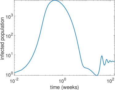
Figure 1: The infected population $I(t;\theta)$ with $\theta={0}$.

5.1.2 Derivative-based GSA

To compute the the partial derivatives $s_{j}(t;\theta)=\frac{\partial y(t;\theta)}{\partial\theta_{j}}$, $j=1,\ldots,8$, needed for DGSM computation, we rely on the so called direct approach; this involves integrating the sensitivity equations [31, 38] along with the ODEs describing the system state. Specifically, we need to integrate the system

$$y^{\prime} =g(y;c(\theta)),\quad y(0)=y_{0},$$

$$s^{\prime}_{i} ={J}{s}_{i}+\frac{\partial g}{\partial\theta_{i}},\quad{s}_{i}(0)={0},\quad i=1,\ldots,{N_{\text{par}}}.$$

Here ${J}$ is the Jacobian $J_{ij}=\frac{\partial g_{i}}{\partial\theta_{j}}=\frac{\partial g_{i}}{\partial c_{j}}\frac{\partial c_{j}}{\partial\theta_{j}}$, $i,j=1,\ldots,{N_{\text{par}}}$. In the present example this results in an “augmented state vector” $[y^{\top}\,s_{1}^{\top}\,\cdots\,s_{8}^{\top}]^{\top}\in\mathbb{R}^{45}$.

First, we consider the pointwise-in-time DGSMs, $\nu_{j}(f(t,\cdot))$, $j=1,\ldots,8$, for $t\in[0,150]$ in Fig. 2 (left). To ensure an accurate estimate of the DGSMs, we approximate the integral over the parameters with a Monte Carlo sample of size $10^{5}$. As seen in Fig. 2 (left), these pointwise-in-time DGSMs are not straightforward to interpret. A clearer picture is obtained by considering

$${\mathfrak{N}}_{j}(I;[0,t]):=\int_{0}^{t}\nu_{j}(I(s,\cdot))\,ds,\quad t\in[0,150],$$

which amounts to computing the functional DGSMs over successively larger time intervals; the results are reported in Fig. 2 (right).

Finally, to get an overall picture, we compute the DGSM-based upper bounds on the functional Sobol’ indices, as given by Theorem 3.3, with $\mathscr{X}=[0,150]$; see Fig. 3, where we report the functional total Sobol’ indices along with the DGSM-based bounds which are computed with Monte Carlo (MC) sample sizes of $10^{5}$ and 100. Note that a small MC sample is very effective in detecting the unimportant parameters.

By Theorem 3.3, we know that a small DGSM-based bound for a given parameter implies the corresponding total Sobol’ index is small, indicating the parameter is unimportant. In the present experiment, we set an importance threshold of $0.05$. A parameter whose DGSM-based bound is smaller than this importance threshold will be considered unimportant. The results reported in Fig. 3 indicate that unimportant parameters are given by $\theta_{j}$ with $j\in\{1,4,5,7\}$. This is consistent with results reported in [4], where the statistical accuracy of the reduced model, obtained by fixing these unimportant parameters was demonstrated numerically. Both panels of Fig. 3 show the same information; however, in the right panel we use a logarithmic scale in the vertical axis to clearly illustrate the bound derived in Theorem 3.3, for the small functional Sobol’ indices.

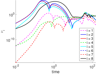
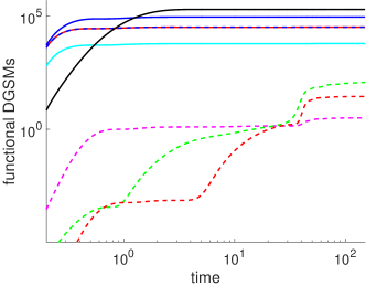
Figure 2: Pointwise-in-time DGSMs $\nu_{j}(I(t,\cdot))$ (left) and functional DGSMs ${\mathfrak{N}}_{j}(I;[0,t])$ (right) for $t\in[0,150]$.

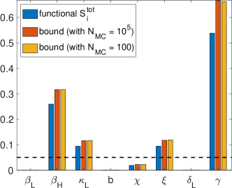
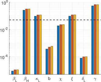
Figure 3: Left: The functional Sobol indices and the corresponding bounds proven in Theorem 3.3 for the cholera model; right: the same information as in the left plot, except we use log-scale on $y$-axis to clearly show $\mathfrak{S}^{\text{tot}}_{j}(I;\mathscr{X})$ and the corresponding bound, for small indices; the dashed black line indicates $y=0.05$ that could be a reasonable tolerance to decide which random input is unimportant.

5.2 Sensitivity analysis in a subsurface flow problem

In this section, we elaborate our proposed approach for sensitivity analysis and dimension reduction on a model problem motivated by subsurface flow applications.

5.2.1 Model description

We consider the following equation modeling the fluid pressure in a single phase flow problem:

(22) $$-\nabla\cdot\Big{(}\frac{\kappa}{\eta}\,\nabla p\Big{)} =b, \quad\text{in }\mathcal{D}$$

$$p =0 \quad\text{on }\Gamma_{D},$$

$$\frac{\kappa}{\eta}\nabla p\cdot n =0, \quad\text{on }\Gamma_{N}$$

The domain is $\mathcal{D}=(-1,1)\times(0,1)$, $\Gamma_{D}$ is the union of the left, bottom, right parts of the boundary, and $\Gamma_{N}$ is the top boundary. The right hand side function $b(x)$ is defined as a sum of mollified point sources, $b(x)=\sum_{i=1}^{4}\alpha_{i}\delta_{x_{i}}(x)$, where

$$\delta_{x_{i}}(x)=\frac{1}{2\pi L}\exp\left\{-\frac{1}{2L}\|x-x_{i}\|_{2}^{2}\right\},$$

with $x_{1}=(-0.6,0.2),x_{2}=(-0.2,0.4)$, and $x_{3}=(0.2,.6)$, and $x_{4}=(0.6,0.8)$. We chose $(\alpha_{1},\alpha_{2},\alpha_{3},\alpha_{4})=(2,5,5,2)$. In this problem, we assume viscosity is $\eta=1$ and consider uncertainties in the permeability field $\kappa$, which is modeled as a log-Gaussian process:

(23) $$\log\kappa(x,\omega)=:a(x,\omega)=\bar{a}(x)+\sigma_{a}z(x,\omega),\quad x\in\mathcal{D},\omega\in\Omega,$$

where $\Omega$ is an appropriate sample space, and $z(x,\omega)$ is a Gaussian process with mean zero and covariance function given by

$$c_{z}(x,y)=\exp\left\{-\frac{|x_{1}-y_{1}|}{\ell_{x}}-\frac{|x_{2}-y_{2}|}{\ell_{y}}\right\},\quad x,y\in\mathcal{D}.$$

In the present example, we use $\ell_{x}=1/2$ and $\ell_{y}=1/4$, implying stronger correlations in the horizontal direction. The covariance operator $\mathcal{C}_{\text{par}}$ is defined by $\mathcal{C}_{\text{par}}u=\int_{\mathscr{X}}c_{z}(\cdot,y)u(y)\,dy$. The mean of the process $\bar{a}(x)$ is adapted from the simulated permeability data from the Society for Petroleum Engineers (SPE) 2001 Comparative Solutions Project [1]; see Fig. 4. For this problem we use $\sigma_{a}=1.6$.

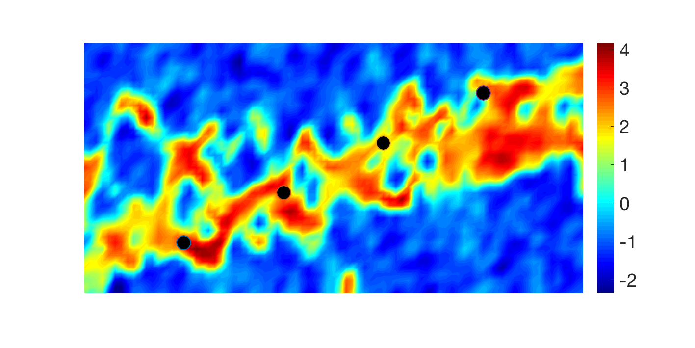
Figure 4: Mean log-permeability field. The black dots indicate point source locations.

We use a truncated KL expansion to represent the log-permeability field:

(24) $$a(x,\omega)\approx\bar{a}(x)+\sum_{k=1}^{N_{\text{par}}}\sqrt{\lambda_{k}(\mathcal{C}_{\text{par}})}\theta_{k}(\omega)e_{k}(x),$$

where $\theta_{k},~{}k=1,2,\ldots,{N_{\text{par}}}$ are independent standard normal random variables, and $\lambda_{k}(\mathcal{C}_{\text{par}})$ and $e_{k}(x)$ are the eigenpairs of the covariance operator $\mathcal{C}_{\text{par}}$ of $a(x,\omega)$ (which is defined in terms of the correlation function $c_{z}$ as before). Note that when using the truncated KL expansion, the uncertainty in the log permeability field is characterized by the random vector $\theta=(\theta_{1},\theta_{2},\ldots,\theta_{N_{\text{par}}})^{\top}\in\mathbb{R}^{N_{\text{par}}}$.

To establish the truncation level, we consider the ratio

$$r_{k}=\frac{\sum_{i=1}^{k}\lambda_{i}}{\sum_{i=1}^{\infty}\lambda_{i}},\quad k=1,2,3,\ldots,$$

where $\lambda_{i}$’s are the eigenvalues of the covariance operator $\mathcal{C}_{\text{par}}$. We depict the normalized eigenvalues, $\lambda_{k}/\lambda_{1}$ in Fig. 5 (left) and plot the ratios $r_{k}$, for $k=1,\ldots,1000$. We find that $r_{k}>0.9$, for $k=126$; thus, we retain ${N_{\text{par}}}=126$ in the KL expansion of the log-permeability field. We will see shortly (see Section 5.2.3) that this is an unnecessarily large parameter dimension for the quantity of interest under study.

As an illustration, in Fig. 6, we show two realizations of the resulting log-permeability field (left) along with the corresponding pressure fields (right) obtained by solving Eq. 22.

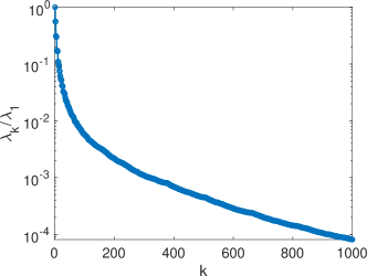
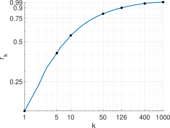
Figure 5: Left: the normalized eigenvalues of the log-permeability field covariance operator; right: the ratios $r_{k}$, for $k=1,\ldots,1000$.

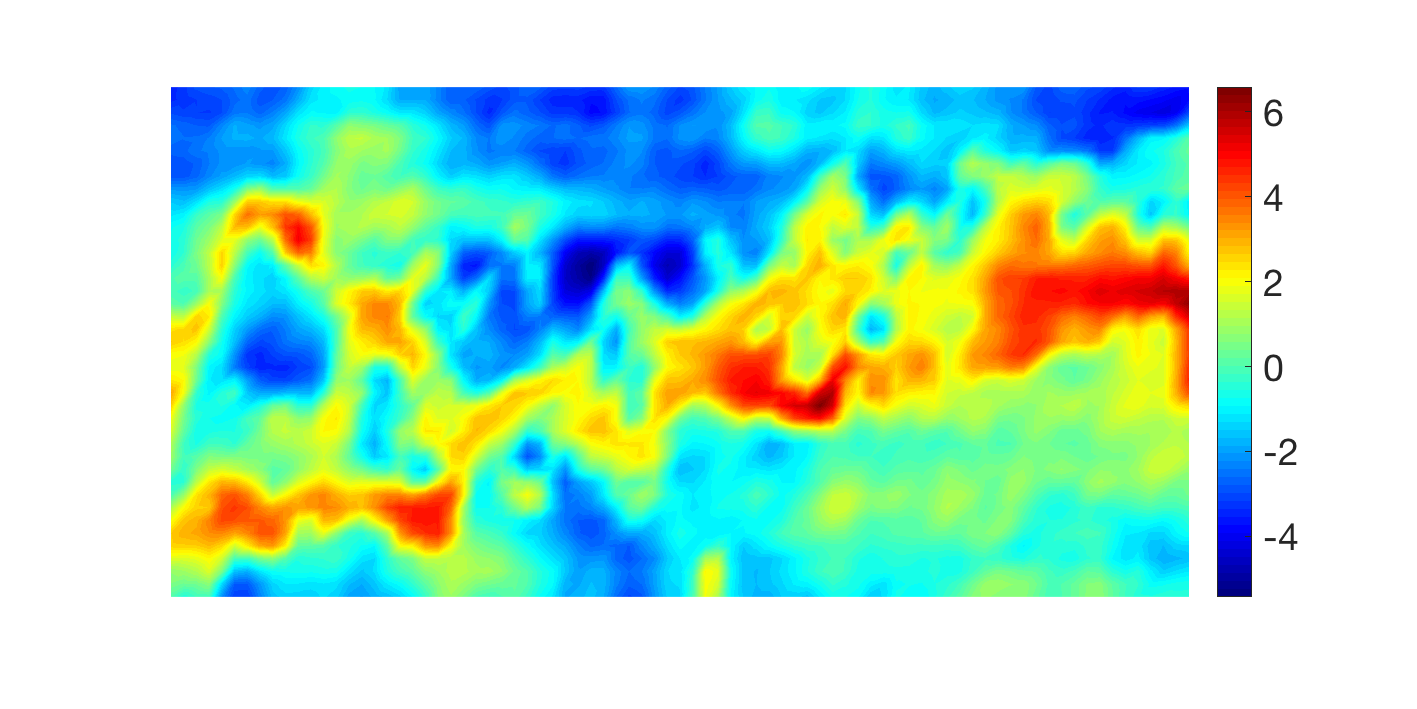
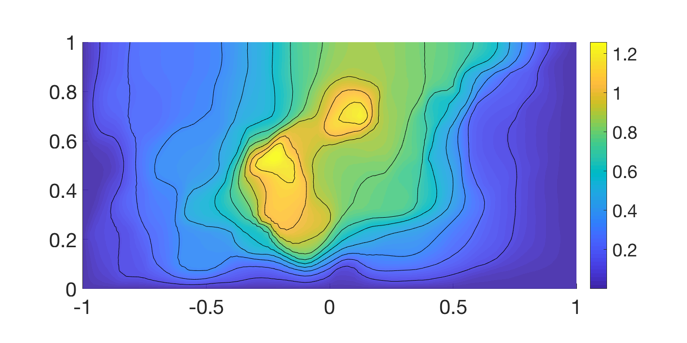
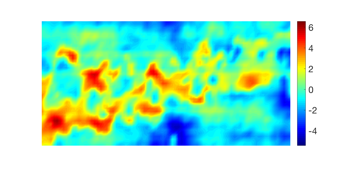
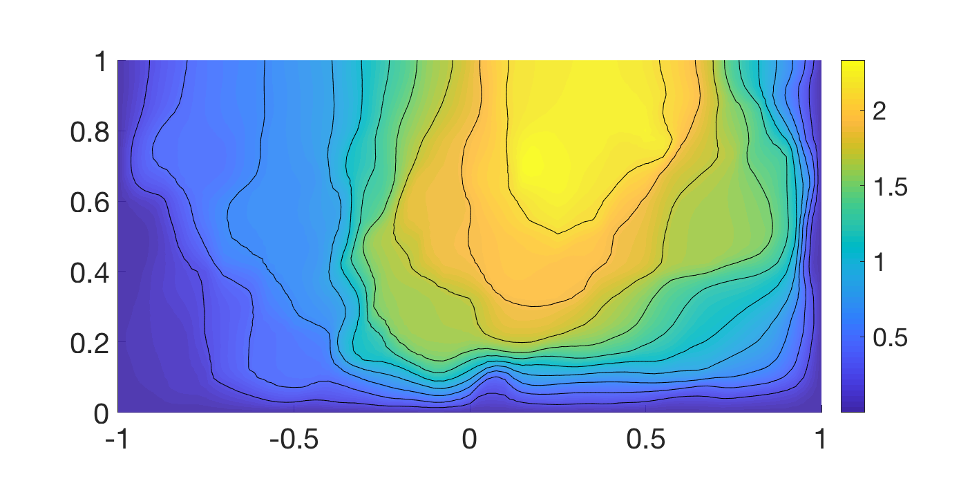
Figure 6: Realizations of the log-permeability field (left), and the corresponding pressure fields (right).

5.2.2 The quantity of interest and its spectral representation

We consider the following quantity of interest:

$$f(x,\theta):={\left.\kern-1.2ptp(x,\theta)\vphantom{\big{|}}\right|_{\Gamma_{N}}}.$$

A few realizations of $f(x,\theta)$ are plotted in Fig. 7 (left). To compute the KL expansion of $f$, we use a sample average approximation of its covariance function, which is then used to solve the discretized generalized eigenvalue problem for its KL modes. The first 30 normalized eigenvalues of the covariance operator of $f$, which we denote by $\mathcal{C}_{\text{qoi}}$, are plotted in Fig. 7 (middle, red color); these correspond to computing the KL expansion of the QoI using sampling with a Monte Carlo (MC) sample of size ${N_{\text{MC}}}=1000$. We also plot the eigenvalues of the log-permeability field covariance operator $\mathcal{C}_{\text{par}}$, in the same plot (blue color); note that the eigenvalues of $\mathcal{C}_{\text{qoi}}$ decay significantly faster than those of $\mathcal{C}_{\text{par}}$, as expected. To assess the impact of the MC sample size on computation of the dominant eigenvalues of $\mathcal{C}_{\text{qoi}}$, we report the normalized eigenvalues of $\mathcal{C}_{\text{qoi}}$ computed using successively larger sample sizes, in Fig. 7 (right). We observe that a sample of size $\mathcal{O}(100)$ can be used for computing the dominant eigenvalues reliably.

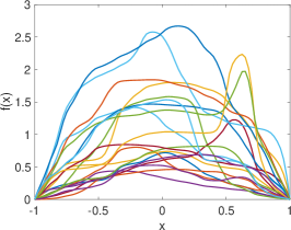
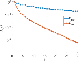
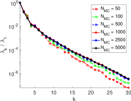
Figure 7: A few realizations of the QoI (left), eigenvalues of the output covariance operator versus those of the log-permeability field (middle). Eigenvalues of the output covariance, with successively larger MC samples sizes for computing the output KLE (right).

The fast decay of eigenvalues of $\mathcal{C}_{\text{qoi}}$ indicates the potential for output dimension reduction. We note four orders of magnitude reduction in the size of the eigenvalues of $\mathcal{C}_{\text{qoi}}$ with only 15 modes in Fig. 7 (right). Hence, we consider a low-rank approximation of $f$,

(25) $$f(x,\theta)\approx\hat{f}(x,\theta)=\bar{f}(x)+\sum_{i=1}^{N_{\text{qoi}}}\sqrt{\lambda_{i}(\mathcal{C}_{\text{qoi}})}f_{i}(\theta)\phi_{i}(x)$$

with ${N_{\text{qoi}}}=15$. While this provides a low-rank approximation to $f$, the dimension of $\theta$ is still high, and is determined by the truncation of the KL expansion of the log-permeability field at ${N_{\text{par}}}=126$. Below, we use global sensitivity analysis to reduce the dimension of $\theta$.

5.2.3 Derivative-based GSA

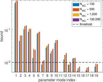
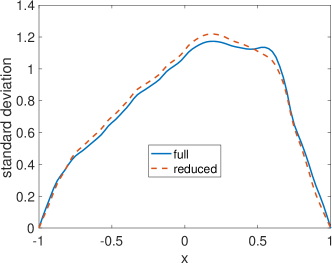
Figure 8: Left: DGSM-based bound in Theorem 3.3 calculated for various sample sizes. Right: standard deviation fields for full model versus that of the reduced model.

We begin by calculating the DGSM-based bounds on functional Sobol’ indices from Theorem 3.3 for $\hat{f}$ defined in Eq. 25. As seen before, this process requires sampling the QoI; we compute the DGSM-based bounds by using MC samples of size ${N_{\text{MC}}}=100,500,1{,}000$, and $100{,}000$. The resulting bounds for the first $19$ parameters are reported in Fig. 8 (left).

Note that Fig. 8 (left) displays the bounds for only the first $19$ modes, because the bounds for the remaining 107 modes were all well below the chosen importance threshold of 0.01. We note that the results calculated with ${N_{\text{MC}}}=500,1{,}000$, and $100{,}000$ provide a consistent classification of important and unimportant parameters. This indicates that in practice, a modest sample size is sufficient for obtaining informative estimates of the DGSM-based bounds from Theorem 3.3.

The computed DGSM-based bounds indicate that the parameter KL modes $\theta_{j}$, with $j\in\{1,2,3,4,5,6,7,8,9,10,12,14\}$ were above the chosen importance threshold of 0.01 and the remaining modes can be fixed at a nominal value of zero. This effectively reduces the parameter dimension from ${N_{\text{par}}}=126$ to ${N_{\text{par}}}=12$. We denote the resulting reduced model, now a function of only $12$ variables, by $f^{r}$. To test that $f^{r}$ reliably captures the variability of the true model $f$, we sample both reduced and full models $10^{5}$ times to compare their statistical properties. In Fig. 8 (right), we compare the standard deviation of the full and reduced models over the spatial domain $\mathscr{X}=[-1,1]$ of the QoI. In Fig. 9 we report PDFs of $f(x,\cdot)$ and $f^{r}(x,\cdot)$, at $x=-0.75,~{}-0.25,~{}0.25,~{}0.75$. We note that the reduced model captures the distribution of the QoI at the considered points closely.

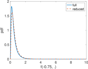
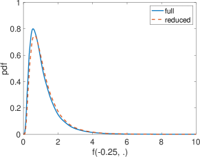
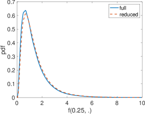
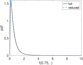
Figure 9: pdf estimate for equally spaced points, $[-1,1]$

5.3 Application to biotransport in tumors

In this section, we apply our derivative-based GSA methods to a biotransport problem. Specifically, we consider biotransport in cancerous tumors with uncertain material properties. We focus on the resulting uncertainties in the pressure field in a spherical tumor when a single needle injection occurs at the center of the tumor.

5.3.1 Model description

Restricting our attention to a 2D cross-section, we consider Darcy’s law constrained by conservation of mass in a 2D physical domain $\mathcal{D}\subset\mathbb{R}^{2}$ given by a circle of radius $R_{\text{tumor}}=5$ mm with an inner circle of radius $R_{\text{needle}}=0.25$ mm, modeling the injection site, removed; see Fig. 10. The inner and outer boundaries of the physical domain $\mathcal{D}$ are denoted by $\Gamma_{\text{N}}$ and $\Gamma_{\text{D}}$, respectively.

Table 2: Model parameters for the biotransport problem.

Parameter	Symbol	Nominal Value [unit]
Permeability	$\kappa$	$0.5~{}[md]$
Viscosity	$\eta$	$8.9\times 10^{-4}~{}[Pa\cdot s]$
Inflow rate	$Q$	$1~{}[mm^{2}/min]$

Figure 10: The domain $\mathcal{D}$. The inner and outer boundaries are equipped with Neumann and Dirichlet boundary conditions and are denoted by $\Gamma_{\text{N}}$ and $\Gamma_{\text{D}}$, respectively.

The fluid pressure $p$ is governed by the following elliptic PDE:

(26) $$-\nabla\cdot\left(\frac{\kappa}{\eta}\nabla p\right) =0\quad\text{in }\mathcal{D},$$

$$p =0\quad\text{on }\Gamma_{\text{D}},$$

$$\nabla p\cdot n =\frac{Q\eta}{2\pi R_{\text{needle}}\kappa}\quad\text{on }\Gamma_{\text{N}}.$$

Here $\kappa$ is the absolute permeability field, $\eta$ is the fluid dynamic viscosity, $Q$ represents the volume flow rate per unit length, and ${n}$ is the outward-pointing normal of the inner boundary $\Gamma_{\text{N}}$. The nominal values for the parameters in Eq. 26 are given in Fig. 10. These values are selected according to those used in previous experimental and numerical studies of fluid transport in tumors [36, 30, 10]. As has been discussed by many researchers, tumor structure can be highly complicated due to its invasive nature. In general, a tumor consists of loosely organized abnormal cells, fibers, vasculature, and lymphatics [9]. This results in randomly formed tumor tissues with structural heterogeneity.

In this subsection, the permeability field is modeled as a log-Gaussian random field as follows. Let $z(x,\omega)$ be a centered Gaussian process with the following covariance function:

(27) $$c_{z}({x},{y})=\exp\left\{-\frac{1}{\ell}\|x-y\|_{1}\right\},\quad x,y\in\mathcal{D},$$

where $\ell>0$ is the correlation length. Then, we define the log-permeability $a=\log\kappa$ as in Eq. 23, where the pointwise mean and variance of the process are given by $\bar{a}\equiv\ln(0.5)+\sigma^{2}_{a}$ and $\sigma^{2}_{a}=0.25$, respectively. Note that $\bar{a}$ is selected to ensure that the mode of the $\kappa$ distribution at each spatial point is $0.5~{}md$, which is the nominal value for $\kappa$ given in Fig. 10. We can represent $a(x,\omega)$ using a truncated KL expansion as in Eq. 24.

5.3.2 The quantity of interest and its spectral representation

We consider the following QoI:

(28) $$f(x,\theta)=\mathcal{Q}p,$$

where, as in Section 4, $\mathcal{Q}$ is the restriction operator to a closed subset $\mathscr{X}$ of $\mathcal{D}$. In this case, $\mathscr{X}$ is an annulus with the inner boundary given by the inner boundary $\Gamma_{\text{N}}$ of $\mathcal{D}$ and with the outer boundary having a radius $R_{out}=1~{}mm$, $2~{}mm$, or $3~{}mm$ (see Fig. 10). The corresponding truncated KL expansion of $f$ reads

(29) $$\hat{f}(x,{\theta}):=\bar{f}(x)+\sum_{k=1}^{{N_{\text{qoi}}}}\sqrt{\lambda_{k}(\mathcal{C}_{\text{qoi}})}f_{k}({\theta})\phi_{k}(x),$$

where the KL modes $f_{i}$ are defined as before, and $\lambda_{k}(\mathcal{C}_{\text{qoi}})$ and $\phi_{k}(x)$ are the eigenpairs of the QoI covariance operator $\mathcal{C}_{\text{qoi}}$.

5.3.3 Derivative-based GSA

As in Section 5.2.3, we calculate the DGSM-based bounds on functional Sobol’ indices from Theorem 3.3 for the QoI defined in Eq. 29 and follow the adjoint-based framework outlined in Section 4. As mentioned previously, a small DGSM-based bound for a given parameter implies that the corresponding functional total Sobol’ index is small and thus, the parameter is deemed unimportant. In the experiments in this section, we set an importance threshold of $0.025$. In Fig. 11, we study the effects of the MC sampling size ${N_{\text{MC}}}$, the KL expansion dimension ${N_{\text{par}}}$ of the input and ${N_{\text{qoi}}}$ of the output, annulus size (i.e., size of $\mathscr{X}$), and correlation length $\ell$ on DGSM-based bounds. Note that Fig. 11 displays the DGSM-based bounds for the first $37$ modes, beyond which the DGSM-based bounds were all below the chosen importance threshold. Below, we explain the numerical experiments reported in Fig. 11, in detail.

In the first test, we examine the effect of the MC sample size ${N_{\text{MC}}}$ as needed in our approach for computing DGSMs (cf. Algorithm 1). Similar to the observation in Section 5.2.3, a modest sample size is sufficient for obtaining informative estimates of the DGSMs. Specifically, we present one set of test results in Fig. 11 (top left). Here, the outer radius of the annulus is $1~{}mm$, the correlation length is $0.5~{}mm$, and we consider an input dimension of ${N_{\text{par}}}=150$, and an output dimension of ${N_{\text{qoi}}}=50$. We observe that a sample size of ${N_{\text{MC}}}~{}=~{}750$ is sufficient for obtaining a reliable estimation of DGSMs-based bounds. Therefore, the MC sample size in the following tests is fixed at ${N_{\text{MC}}}~{}=~{}750$.

We then test the effects of the annulus size and correlation length on DGSMs. In these tests, the input and output dimensions are ${N_{\text{par}}}=150$ and ${N_{\text{qoi}}}=50$, respectively. From Fig. 11 (top right and bottom left), we observe that when the annulus size increases or the correlation length decreases, the QoI is sensitive to more KL terms of the input. Interestingly, most of these sensitive parameters are from relatively high-order terms. For example, as shown in Fig. 11 (bottom left), when the correlation length decreases from $2.0~{}mm$ to $0.5~{}mm$, the importance of KL modes $\theta_{j}$, with $j\in\{9,10,17,22,23\}$ gradually grow. Implication of such issues on reduced-order modeling (ROM) will be discussed in the next section. Next, we examine the impact of increasing ${N_{\text{par}}}$ and ${N_{\text{qoi}}}$. As seen in Fig. 11 (bottom right), increasing the input and output dimensions beyond the selected values of ${N_{\text{par}}}=150$ and ${N_{\text{qoi}}}=50$ does not result in noticeable changes in DGSM estimates.

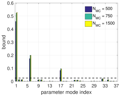
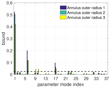
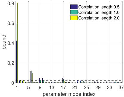
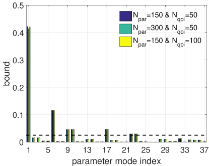
Figure 11: The functional DGSM-based bounds of pressure fields in a tumor with uncertain permeability. Top left: Convergence study with the MC sample size $N_{MC}~{}=~{}500,~{}750,$ and $1500$. Top right: Comparison of DGSM-based bounds for different annulus sizes, namely the annulus outer radii of $1~{}mm$, $2~{}mm$, and $3~{}mm$. Bottom left: Comparison of DGSM-based bounds for different correlation lengths, namely $0.5~{}mm$, $1~{}mm$, and $2~{}mm$. Bottom right: DGSM-based bounds calculated with different combinations of the KL expansion dimensions of the input and output.

5.3.4 Insights on ROM assisted by DGSMs

From the global sensitivity analysis, we find that the QoI is only sensitive to several selected KL terms of the input. This can be used to guide ROM based on DGSMs. In this section, we compare two ROM approaches: one is based on the GSA with DGSMs (termed as DGSM-based ROM) and the other is based on directly selecting the first $k$-terms of the KL expansion of the random input field (termed as KL-based ROM). Generally, the reduced-order model of the input can be written as follows:

(30) $$\tilde{a}(x,\omega)=\bar{a}(x)+\sum_{k\in\mathcal{S}}\sqrt{\lambda_{k}(\mathcal{C}_{\text{par}})}\theta_{k}(\omega)e_{k}(x),$$

where $\mathcal{S}$ is the set which consists of the indices of the KL terms used in ROM. We evaluate the performance of the two ROM methods on recovering the PDFs of pressures at different locations in the flow field.

As shown in Fig. 12, we select three points on the mesh with different distances from the center of the domain: the point $P_{1}$ is on the inner boundary with a large relative standard deviation (RSD) of the pressure ($RSD=0.143$); the point $P_{2}$ is close to the inner boundary with a moderate RSD ($RSD=0.105$); and the point $P_{3}$ is far from the inner boundary with a relatively small RSD ($RSD=0.0845$). In the DGSM-based ROM, the first $n$ KL terms which the QoI is most sensitive to are used to reconstruct the reduced-order model of the pressure field. In the KL-based ROM, the first $n$ KL terms, corresponding to the $n$ largest eigenvalues of the input covariance operator, are used to reconstruct the reduced-order model. An MC sampling approach is used to construct PDFs from the full model, which includes all the KL terms, and those from the reduced-order models with different fidelities. The case with a small correlation length ($\ell=0.5~{}mm$) and a large annulus size ($R_{out}=3~{}mm$) is studied here. An MC sample of size $6000$ was found sufficient for constructing the PDFs.

From Fig. 13, we observe that at $P_{1}$, where the pressure variance is large, the reduced-order model with only the first seven most sensitive KL terms can nearly recover the PDF of the full model. Its performance is comparable to that of the KL-based ROM with the first 30 KL terms. This is not a surprise, because, as seen from the last figure in Fig. 11, the first seven most sensitive KL terms $\theta_{j}$, with $j\in\{1,6,9,10,17,22,23\}$, are within the first 30 KL terms used in the KL-based ROM. Similar conclusions can be drawn at $P_{2}$ where a moderate pressure variance is observed. At $P_{3}$, we find that the DGSM-based ROM with the first seven most sensitive KL terms does not recover the PDF well; however, the PDFs obtained using the DGSM-based ROMs with more KL terms, such as that with the first 15, 30 and 45 most sensitive KL terms, gradually approach the PDF of the full model. On the other hand, with the same number of KL terms, the KL-based ROM makes very slow progress towards the full model PDF. All these observations indicate that the DGSM-based ROM can be a much more efficient reduced-order modeling approach than the KL-based ROM that involves a priori truncation of the input field KL terms.

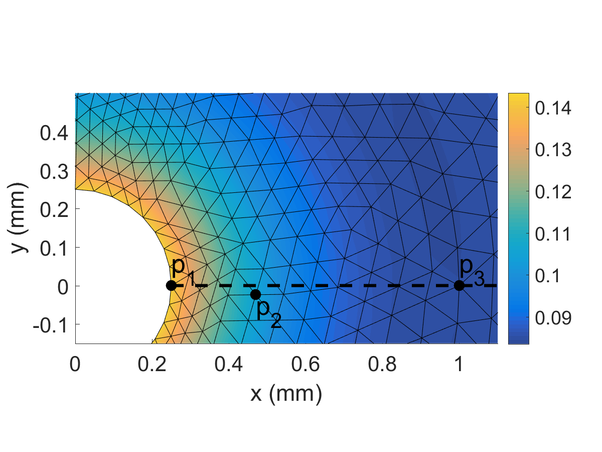
Figure 12: Distribution of the points where PDFs of pressures are extracted, and the corresponding RSD field (contour).

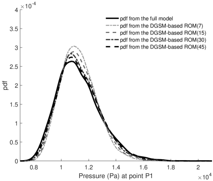
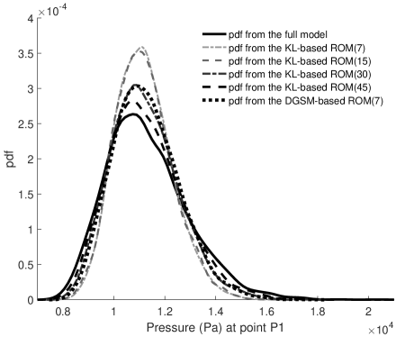
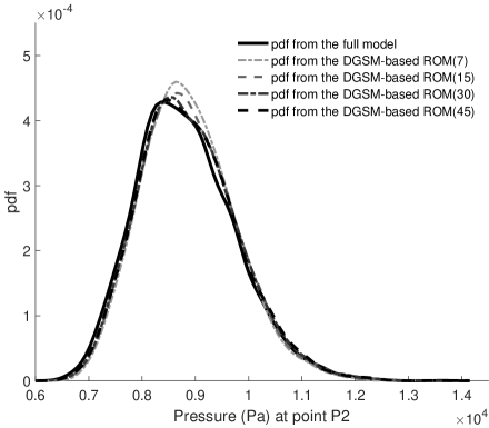
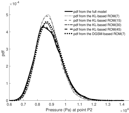
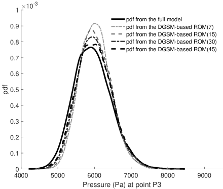
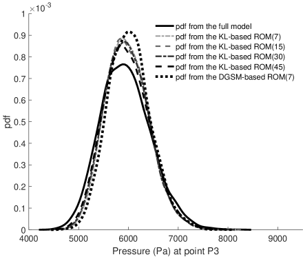
Figure 13: Comparison of PDFs constructed from the DGSM-based ROM (left column) and KL-based ROM (right column) with variable fidelity at points $P_{1}$, $P_{2}$ and $P_{3}$.

6 Conclusions

We have presented a mathematical framework for GSA of models with functional outputs, and have proposed an efficient computational method for identifying unimportant inputs that is suitable for models with high-dimensional parameters. The latter is done by combining the proposed functional DGSMs, “low-rank” KL expansions of output QoIs, and adjoint-based gradient computation. In particular, the computational complexity of the proposed approach, in terms of the number of required model evaluations, does not scale with dimension of the parameter. The effectiveness of the proposed framework is illustrated numerically in applications from epidemiology, subsurface flow, and biotransport.

The proposed approach is effective in finding unimportant input parameters. This approach also paves the way for an efficient surrogate modeling approach: the low-rank KL expansion of the model output can be used to construct efficient-to-evaluate surrogate models by computing surrogate models for the KL modes, in the reduced parameter space, which is identified using the functional DGSMs. The latter can be done using various methods including orthogonal polynomial approximations [28, 48, 40], multivariate adaptive regression splines [16], or active subspace approaches [11]. We mention that active subspace methods have also been used directly for dimension reduction in models with vectorial outputs. Namely, [49] presents a gradient-based input dimension reduction method for such models. The method proposed in [49] finds a set of important directions in the input parameter space by considering ridge approximations of the model output and by minimizing an upper bound on the approximation error. The approach in [49] is related to the present work when the goal of GSA is input dimension reduction.

In future work, we seek to investigate generalizations to cases of models with correlated inputs. While the proposed DGSMs can be computed for such models in the same way, the corresponding variance-based indices need to be generalized. We are also interested in applying the proposed method to more complex physical applications such as multiphase flow in geological formations.

Appendix A Proof of Proposition 2.3

We will need the following key lemma, which is is based on the arguments in [44].

Lemma A.1.

For every $s\in\mathscr{X}$, $\int_{\Theta_{U^{c}}}\varepsilon\left({f};s;{\eta}\right)\mu(d\eta)=2D_{U^{c}}^{\text{tot}}(f;s)$.

Proof A.2.

Let $s\in\mathscr{X}$ be fixed. Consider the ANOVA decomposition of $f(s,\theta)$, as defined in Eq. 2:

$$f(s,\theta)=f_{0}(s)+f_{1}(s,\theta_{U})+f_{2}(s,\theta_{U^{c}})+f_{12}(s,\theta_{U},\theta_{U^{c}}).$$

By substituting this into the expression for $\varepsilon\left({f};s;{\eta}\right)$ and simplifying we have

(31) $$\varepsilon\left({f};s;{\eta}\right)=\int_{\Theta}\big{[}f_{2}(s,\theta_{{U^{c}}})+f_{12}(s,\theta_{U},\theta_{U^{c}})-f_{2}(s,\eta)-f_{12}(s,\theta_{U},\eta)\big{]}^{2}\mu\,(d\theta).$$

Using the properties of ANOVA [44, 42],

$$\int_{\Theta_{U^{c}}}f_{2}(s,\theta_{{U^{c}}})\,\mu(d\theta_{U^{c}})=\int_{\Theta_{U^{c}}}f_{12}(s,\theta_{U},\theta_{U^{c}})\,\mu(d\theta_{U^{c}})=\int_{\Theta_{U}}f_{12}(s,\theta_{U},\theta_{U^{c}})\,\mu(d\theta_{U})=0,$$

we can simplify Eq. 31 to get, for a fixed $\eta\in{\Theta_{U^{c}}}$,

$$\varepsilon\left({f};s;{\eta}\right) =\int_{\Theta}\big{[}f_{2}^{2}(s,\theta_{{U^{c}}})+f_{12}^{2}(s,\theta_{U},\theta_{U^{c}})+f_{2}^{2}(s,\eta)+f_{12}^{2}(s,\theta_{U},\eta)\big{]}\,\mu(d\theta)$$

$$=D_{U^{c}}(f;s)+D_{U^{c},U}(f;s)+f_{2}^{2}(s,\eta)+\int_{\Theta_{U}}f_{12}^{2}(s,\theta_{U},\eta)\,\mu(d\theta_{U}).$$

Integrating the above expression over $\Theta_{U^{c}}$ gives the desired result.

• First note that the denominator is a constant and

  (32) $$\int_{\mathscr{X}}\int_{\Theta}f(s,\theta)^{2}\,\mu(d\theta)ds=\int_{\mathscr{X}}\Bigg{[}D(f;s)+\Big{(}\int_{\Theta}f(s,\theta)\mu(d\theta)\Big{)}^{2}\Bigg{]}\,ds\geq\int_{\mathscr{X}}D(f;s)ds.$$

  Next, consider the expectation of the numerator in Eq. 4:

  (33) $$\int_{\Theta_{U^{c}}}\int_{\mathscr{X}}\int_{\Theta}(f(s,\theta)-f^{(\eta)}(s,\theta_{U}))^{2}\,\mu(d\theta)ds\mu(d\eta)=\int_{\Theta_{U^{c}}}\int_{\mathscr{X}}\varepsilon\left({f};s;{\eta}\right)\,ds\mu(d\eta)\\ =\int_{\mathscr{X}}\int_{\Theta_{U^{c}}}\varepsilon\left({f};s;{\eta}\right)\,\mu(d\eta)\,ds=2\int_{\mathscr{X}}D_{U^{c}}^{\text{tot}}(f;s),$$

  where changing the order of integration is justified by Tonell’s theorem, and the last equality follows from Lemma A.1. The desired result follows from Eq. 33 and Eq. 32.

Appendix B Proof of Propositions 3.1 and 3.5

We recall the following result: if a random variable $X$ satisfies $a\leq X\leq b$ and $\mathrm{E}\left\{{X}\right\}=m$, then

(34) $$\mathrm{Var}\left\{{X}\right\}\leq(b-m)(m-a)\leq(b-a)^{2}/4.$$

The first inequality is known as the Bhatia–Davis inequality [7]. The second inequality gives a corollary of the Bhatia-Davis inequality, known as Popoviciu’s inequality, that says $\mathrm{Var}\left\{{X}\right\}\leq(b-a)^{2}/4$, for a random variable satisfying $a\leq X\leq b$.

• Note that clearly $a_{j}\leq\nu_{j}(g)\leq b_{j}$, for $j=1,\ldots,{N_{\text{par}}}$. Applying the inequality Eq. 34 with $X=\big{(}\frac{\partial g}{\partial\theta_{j}}\big{)}^{2}$ and $(b,m,a)=(b_{j},\nu_{j}(g),a_{j})$, $j=1,\ldots,{N_{\text{par}}}$, we obtain $\mathrm{Var}\big{\{}\big{(}\frac{\partial g}{\partial\theta_{j}}\big{)}^{2}\big{\}}\leq\big{(}b_{j}-\nu_{j}(g)\big{)}\big{(}\nu_{j}(g)-a_{j}\big{)}\leq\frac{1}{4}(b_{j}-a_{j})^{2}$. Therefore, for $j=1,\ldots,{N_{\text{par}}}$,

  $$\mathrm{Var}\left\{{\nu_{j}^{({N_{\text{MC}}})}(g)}\right\}=\frac{1}{{N_{\text{MC}}}}\mathrm{Var}\left\{{\Big{(}\frac{\partial g}{\partial\theta_{j}}\Big{)}^{2}}\right\}\leq\frac{1}{{N_{\text{MC}}}}\big{(}b_{j}-\nu_{j}(g)\big{)}\big{(}\nu_{j}(g)-a_{j}\big{)}\leq\frac{1}{4{N_{\text{MC}}}}(b_{j}-a_{j})^{2}.$$

• First note that ${\mathfrak{N}}_{j}^{({N_{\text{MC}}})}(f;\mathscr{X})$ is indeed an estimator for ${\mathfrak{N}}_{j}(f;\mathscr{X})$. This is seen by noting that, using Tonelli’s theorem,

  $${\mathfrak{N}}_{j}(f;\mathscr{X})=\int_{\mathscr{X}}\nu_{j}(f;s)\,ds=\int_{\mathscr{X}}\int_{\Theta}\Big{(}\frac{\partial f}{\partial\theta_{j}}(s,\theta)\Big{)}^{2}\mu(d\theta)ds=\int_{\Theta}\int_{\mathscr{X}}\Big{(}\frac{\partial f}{\partial\theta_{j}}(s,\theta)\Big{)}^{2}ds\,\mu(d\theta).$$

  Then, applying Popoviciu’s inequality to the random variable $G_{j}(\theta)=\int_{\mathscr{X}}\Big{(}\frac{\partial f}{\partial\theta_{j}}(s,\theta)\Big{)}^{2}\,ds$, which satisfies $\|a_{j}\|_{L^{1}(\mathscr{X})}\leq G_{j}\leq\|b_{j}\|_{L^{1}(\mathscr{X})}$, gives:

  $$\mathrm{Var}\left\{{G_{j}}\right\}\leq\frac{1}{4}\left(\|b_{j}\|_{L^{1}(\mathscr{X})}-\|a_{j}\|_{L^{1}(\mathscr{X})}\right)^{2}\leq\frac{1}{4}\|b_{j}-a_{j}\|_{L^{1}(\mathscr{X})}^{2},\quad j=1,\ldots,{N_{\text{par}}},$$

  where we also used the reverse triangle inequality. This completes the proof.

References

• [1] 2001 SPE comparative solution project. https://www.spe.org/web/csp/datasets/set02.htm, 2000. Accessed: September 19, 2018.
• [2] R. J. Adler, The geometry of random fields, SIAM, 2010.
• [3] A. Alexanderian, On spectral methods for variance based sensitivity analysis, Probab. Surv., 10 (2013), pp. 51–68.
• [4] A. Alexanderian, P. Gremaud, and R. Smith, Variance-based sensitivity analysis for time-dependent processes, In review (arXiv: https://arxiv.org/abs/1711.08030), (2018).
• [5] A. Alexanderian, W. Reese, R. C. Smith, and M. Yu, Efficient uncertainty quantification for biotransport in tumors with uncertain material properties, in ASME 2018 International Mechanical Engineering Congress and Exposition, American Society of Mechanical Engineers, 2018, pp. V003T04A033–V003T04A033.
• [6] A. Alexanderian, L. Zhu, M. Salloum, R. Ma, and M. Yu, Investigation of biotransport in a tumor with uncertain material properties using a non-intrusive spectral uncertainty quantification method, J. Biomech. Eng., (2017), pp. 091006–1–091006–11.
• [7] R. Bhatia and C. Davis, A better bound on the variance, Amer. Math. Monthly, 107 (2000), pp. 353–357.
• [8] K. Campbell, M. D. McKay, and B. J. Williams, Sensitivity analysis when model outputs are functions, Reliability Engineering & System Safety, 91 (2006), pp. 1468–1472.
• [9] W. H. Clark, Tumour progression and the nature of cancer, Br J Cancer, 64 (1991).
• [10] W. H. Clark, Biphasic finite element model of solute transport for direct infusion into nervous tissue, Annals of Biomedical Engineering, 35 (2007), pp. 2145––2158.
• [11] P. G. Constantine, Active subspaces, vol. 2 of SIAM Spotlights, Society for Industrial and Applied Mathematics (SIAM), Philadelphia, PA, 2015. Emerging ideas for dimension reduction in parameter studies.
• [12] P. G. Constantine and P. Diaz, Global sensitivity metrics from active subspaces, Reliability Engineering & System Safety, 162 (2017), pp. 1–13.
• [13] P. G. Constantine, E. Dow, and Q. Wang, Active subspace methods in theory and practice: applications to kriging surfaces, SIAM Journal on Scientific Computing, 36 (2014), pp. A1500–A1524.
• [14] T. Crestaux, O. L. Maitre, and J.-M. Martinez, Polynomial chaos expansion for sensitivity analysis, Reliability Engineering & System Safety, 94 (2009), pp. 1161 – 1172. Special Issue on Sensitivity Analysis.
• [15] G. B. Folland, Real analysis, Pure and Applied Mathematics (New York), John Wiley & Sons, Inc., New York, second ed., 1999. Modern techniques and their applications, A Wiley-Interscience Publication.
• [16] J. H. Friedman, Multivariate adaptive regression splines, The Annals of Statistics, 19 (1991), pp. 1–141. With discussion and a rejoinder by the author.
• [17] F. Gamboa, A. Janon, T. Klein, A. Lagnoux, et al., Sensitivity analysis for multidimensional and functional outputs, Electronic Journal of Statistics, 8 (2014), pp. 575–603.
• [18] L. L. Gratiet, S. Marelli, and B. Sudret, Metamodel-based sensitivity analysis: polynomial chaos expansions and gaussian processes, in Handbook of Uncertainty Quantification, R. Ghanem, D. Higdon, and H. Owhadi, eds., Springer, 2017.
• [19] J. Hart, A. Alexanderian, and P. Gremaud, Efficient computation of sobol’ indices for stochastic models, SIAM J. Sci. Comput., 39 (2017), pp. A1514–A1530.
• [20] D. M. Hartley, J. G. J. Morris, and D. L. Smith, Hyperinfectivity: a critical element in the ability of v. cholerae to cause epidemics?, PLoS medicine, 3 (2005).
• [21] T. Hsing and R. Eubank, Theoretical foundations of functional data analysis, with an introduction to linear operators, John Wiley & Sons, 2015.
• [22] W. Ji, J. Wang, O. Zahm, Y. M. Marzouk, B. Yang, Z. Ren, and C. K. Law, Shared low-dimensional subspaces for propagating kinetic uncertainty to multiple outputs, Combustion and Flame, 190 (2018), pp. 146–157.
• [23] S. Kucherenko and B. Iooss, Derivative-based global sensitivity measures, in Handbook of Uncertainty Quantification, R. Ghanem, D. Higdon, and H. Owhadi, eds., Springer, 2017.
• [24] S. Kucherenko, M. Rodriguez-Fernandez, C. Pantelides, and N. Shah, Monte carlo evaluation of derivative-based global sensitivity measures, Reliability Engineering & System Safety, 94 (2009), pp. 1135–1148.
• [25] M. Lamboni, B. Iooss, A.-L. Popelin, and F. Gamboa, Derivative-based global sensitivity measures: General links with sobol’ indices and numerical tests, Mathematics and Computers in Simulation, 87 (2013), pp. 45–54.
• [26] M. Lamboni, H. Monod, and D. Makowski, Multivariate sensitivity analysis to measure global contribution of input factors in dynamic models, Reliability Engineering & System Safety, 96 (2011), pp. 450–459.
• [27] P. D. Lax, Functional Analysis, John Wiley & Sons, 2002.
• [28] O. P. Le Maître and O. M. Knio, Spectral methods for uncertainty quantification, Springer, New York, 2010. With applications to computational fluid dynamics.
• [29] M. Loève, Probability theory. I, Springer-Verlag, New York-Heidelberg, fourth ed., 1977. Graduate Texts in Mathematics, Vol. 45.
• [30] R. Ma, D. Su, and L. Zhu, Multiscale simulation of nanopartical transport in deformable tissue during an infusion process in hyperthermia treatments of cancers., in Nanoparticle Heat Transfer and Fluid Flow, Computational & Physical Processes in Mechanics & Thermal Science Series, W. J. Minkowycz, E. Sparrow, and J. P. Abraham, eds., vol. 4, CRC Press, Taylor & Francis Group, 2012.
• [31] T. Maly and L. R. Petzold, Numerical methods and software for sensitivity analysis of differential-algebraic systems, Applied Numerical Mathematics, 20 (1996), pp. 57–79.
• [32] A. Marrel, N. Saint-Geours, and M. De Lozzo, Sensitivity analysis of spatial and/or temporal phenomena, in Handbook of Uncertainty Quantification, R. Ghanem, D. Higdon, and H. Owhadi, eds., Springer, 2017.
• [33] MATLAB, version 8.6.0.267246 (r2015b), 2015.
• [34] J. Mercer, Functions of positive and negative type, and their connection with the theory of integral equations, Philosophical Transactions of the Royal Society of London. Series A, Containing Papers of a Mathematical or Physical Character, (1909), pp. 415–446.
• [35] C. Prieur and S. Tarantola, Variance-based sensitivity analysis: Theory and estimation algorithms, in Handbook of Uncertainty Quantification, R. Ghanem, D. Higdon, and H. Owhadi, eds., Springer, 2017, pp. 1217–1239.
• [36] M. Salloum, R. Ma, D. Weeks, and L. Zhu, Controlling nanoparticle delivery in magnetic nanoparticle hyperthermia for cancer treatment: experimental study in agarose gel, International Journal of Hyperthermia, 24 (2008), pp. 337–345.
• [37] A. Saltelli, K. Chan, E. M. Scott, et al., Sensitivity analysis, vol. 1, Wiley New York, 2000.
• [38] A. Sandu, D. N. Daescu, and G. R. Carmichael, Direct and adjoint sensitivity analysis of chemical kinetic systems with kpp: Part i—theory and software tools, Atmospheric Environment, 37 (2003), pp. 5083–5096.
• [39] K. Sargsyan, Surrogate models for uncertainty propagation and sensitivity analysis, in Handbook of uncertainty quantification, R. Ghanem, D. Higdon, and H. Owhadi, eds., Springer, 2017.
• [40] R. Smith, Uncertainty quantification, theory, implementation, and applications, SIAM, 2013.
• [41] I. Sobol, Estimation of the sensitivity of nonlinear mathematical models, Matematicheskoe Modelirovanie, 2 (1990), pp. 112–118.
• [42] I. Sobol, Global sensitivity indices for nonlinear mathematical models and their Monte Carlo estimates, Mathematics and Computers in Simulation, 55 (2001), pp. 271–280. The Second IMACS Seminar on Monte Carlo Methods.
• [43] I. Sobol’ and S. Kucherenko, Derivative based global sensitivity measures and their link with global sensitivity indices, Mathematics and Computers in Simulation, 79 (2009), pp. 3009–3017.
• [44] I. Sobol, S. Tarantola, D. Gatelli, S. Kucherenko, and W. Mauntz, Estimating the approximation error when fixing unessential factors in global sensitivity analysis, Reliability Engineering & System Safety, 92 (2007), pp. 957–960.
• [45] B. Sudret, Global sensitivity analysis using polynomial chaos expansions, Reliability Engineering & System Safety, 93 (2008), pp. 964 – 979.
• [46] M. Vohra, A. Alexanderian, C. Safta, and S. Mahadevan, Sensitivity-driven adaptive construction of reduced-space surrogates, Journal of Scientific Computing, in press (2018).
• [47] H. Xiao and L. Li, Discussion of paper by matieyendou lamboni, hervé monod, david makowski “multivariate sensitivity analysis to measure global contribution of input factors in dynamic models”, reliab. eng. syst. saf. 99 (2011) 450–459, Reliability Engineering & System Safety, 147 (2016), pp. 194–195.
• [48] D. B. Xiu, Numerical methods for stochastic computations, Princeton University Press, Princeton, NJ, 2010. A spectral method approach.
• [49] O. Zahm, P. Constantine, C. Prieur, and Y. Marzouk, Gradient-based dimension reduction of multivariate vector-valued functions. Preprint, https://arxiv.org/abs/1801.07922, 2018.