Filaments in VIPERS: galaxy quenching in the infalling regions of groups

Abstract

We study the quenching of galaxies in different environments and its evolution in the redshift range $0.43\leq z\leq 0.89$. For this purpose, we identify galaxies inhabiting in filaments, the isotropic infall region of groups, the field, and groups in the VIMOS Public Extragalactic Redshift Survey (VIPERS). We classify galaxies as quenched (passive), through their $NUV-r$ vs. $r-K$ colours. We study the fraction of quenched galaxies ($F_{r}$) as a function of stellar mass and environment at two redshift intervals. Our results confirm that stellar mass is the dominant factor determining galaxy quenching over the full redshift range explored. We find compelling evidence of evolution in the quenching of intermediate mass galaxies $(9.3\leq\log(M_{\star}/M_{\odot})\leq 10.5)$ for all environments. For this mass range, $F_{r}$ is largest for galaxies in groups, and smallest for galaxies in the field, while galaxies in filaments and in the isotropic infall regions appear to have intermediate values with the exception of the high redshift bin, where the latter show similar fraction of quenched galaxies as in the field. Galaxies in filaments are systematically more quenched than their counterparts infalling from other directions, in agreement to similar results found at low redshift. The least massive galaxies in our samples, do not show evidence of internal or environmental quenching.

1 Introduction

The large-scale structure of the Universe in the $\Lambda$CDM model is characterised by the anisotropic structure of the matter distribution, where we observe walls, filaments and their nodes. In the nodes galaxy clusters and groups are observed (Bond et al., 1996). Filaments trace the cosmic web connecting the nodes framing walls separated by large voids (Aragón-Calvo et al., 2010). After galaxy clusters and groups, filaments constitute the densest environment and can account for up to $\sim 40\%$ of the Universe’s mass (Aragón-Calvo et al., 2010).

Several algorithms have been developed to identify filaments in the galaxy distribution. Some of them identify filaments as ridges in the density field (e.g. Novikov et al. 2006; Aragón-Calvo et al. 2007; Sousbie 2011; Cautun et al. 2013). Other algorithms use a minimal spanning tree (Barrow et al., 1985) method instead (e.g. Colberg 2007; Alpaslan et al. 2014). Filaments are also detected as overdensities in the galaxy distribution between pairs of clusters (Pimbblet, 2005), or groups (Martínez et al., 2016).For a detailed comparison of the different web finders, see Cautun et al. (2014) and references therein. Using numerical simulations, these authors also studied the evolution of the cosmic web and found that while most filaments have been in place since $z\sim~{}0.5$, they have been evolving rapidly at higher redshift.

It is well known that galaxy properties strongly depend on stellar mass and environment (e.g., Dressler 1980; Gómez et al. 2003; Martínez et al. 2008). Galaxy properties in clusters and groups have been studied thoroughly at different redshifts (e.g. Martínez & Muriel 2006; Martínez et al. 2008; Wilman et al. 2009; Kovač et al. 2010; Presotto et al. 2012; Cucciati et al. 2017; Coenda et al. 2018), however, the study of galaxies inhabiting the region between two groups/cluster (filament region) have not been as widely studied.

The Galaxy And Mass Assembly (Driver et al. 2009, GAMA) survey of the nearby Universe has been extensively used to study the properties of galaxies on large-scale environments. Eardley et al. (2015) investigated the galaxy luminosity function and found that the luminosity function’s characteristic magnitude brightens 0.5 mag from voids to knots (groups/clusters). On the other hand, Alpaslan et al. (2016) found that the stellar mass is the primary factor to predict the star formation rate (SFR), being the large-scale environment a second order parameter (see also Alpaslan et al. 2015). Also using GAMA, Kraljic et al. (2018) investigated the role of the cosmic web in shaping galaxy properties. They found that the fraction of red galaxies increases when approaching nodes and filaments. Using the Sloan Digital sky Survey (SDSS), Chen et al. (2017) studied the effect of filaments on galaxy properties. They found that a red galaxy or a high-mass galaxy tends to reside closer to filaments than a blue or low-mass galaxy.

At intermediate redshifts, Zhang et al. (2013) studied the colour of galaxies located in between pairs of clusters in the range $0.12\leq z\leq 0.4$ and detect an evolution in the blue fraction of filament galaxies that is not observed in clusters. They also found that richer clusters are connected to richer filaments. Martínez et al. (2016) studied the effects of environment upon galaxies infalling into groups in the SDSS DR7 (Abazajian et al., 2009) by distinguishing whether they are in filaments (filament galaxies, hereafter FG) or falling from other directions (isotropic infalling galaxies, hereafter IG). They show evidence of galaxy preprocessing in the infall region of groups, and a distinct action of the filament environment upon galaxies. FG and IG galaxies differ from field galaxies and galaxies in groups in terms of their luminosity function and their specific star formation rate. The authors found that, while the luminosity function of FG and IG galaxies are similar, they are intermediate between the luminosity function of field galaxies and that of galaxies in groups. They also found systematic lower values of specific star formation rate of FG compared to IG, thus providing evidence that galaxies infalling alongside filaments have experienced stronger environmental effects than galaxies infalling from other directions.

At higher redshifts, Darvish et al. (2014) studied a sample of $H_{\alpha}$ emitting star forming galaxies at $z$ = $0.845$ in the COSMOS field (Scoville et al., 2007). They show an enhancement of star formation activity in filaments compared to denser regions (cluster) which they explain in terms of galaxy – galaxy interactions. Laigle et al. (2018), using a sample of galaxies from the COSMOS field, with photometric redshifts $0.5\leq z_{\rm phot}\leq 0.9$, found that passive galaxies are more confined towards the core of the filament, in contrast to star-forming ones. Malavasi et al. (2017) identified filaments in the final data release of the VIMOS Public Extragalactic Redshift Survey (VIPERS, Guzzo et al. 2014), finding a significant segregation in the sense of the most massive galaxies likely to be closer to filaments. Davidzon et al. (2016) studied how the environment shapes the stellar mass function using VIPERS. They focused on the large scale density and found that the stellar mass function evolves in high densities regions, while it stays nearly constant in low-density environments.

Just et al. (2015), studied galaxies in the infall regions of 21 cluster at intermediate redshift ($0.4\leq z\leq 0.8$) from the ESO Distant Cluster Survey (White et al., 2005). They found that the fraction of red galaxies in the infall region is intermediate to that in clusters and in the field, suggesting a preprocessing of the properties related to the star formation outside the virial radius.

In this paper, we search for filaments defined between pairs of groups at redshifts $0.43\leq z\leq 0.9$ in the final data release of VIPERS (PDR-2, Scodeggio et al. 2018) in order to study the effects of environment in quenching star formation in galaxies infalling into groups. Our goal is to statistically compare galaxies in the outskirts of groups distinguishing between those that are in regions where filaments are likely to be present, and those that are not. It is out of the scope of this paper to construct a complete catalogue of filaments, or to assess univocally if a particular galaxy belongs to a filament or not.

This article is organised as follows: we describe the galaxy data in Sect. 2; Sect. 3 deals with the identification of groups and filaments; in Sect. 4 we compare the fraction of passive galaxies in groups, field, filaments and the isotropic infalling region, and its redshift evolution. We discuss the implications of our results in this section as well. Finally, we summarise our main results in Sect. 5. Throughout the paper we assume a flat cosmology with density parametres $\Omega_{\rm m}=0.30$, $\Omega_{\Lambda}=0.70$, and a Hubble’s constant $H_{0}=70$ km s^-1 Mpc^-1. Unless otherwise specified, all magnitudes and colours are in the Vega system.

2 Data

To identify groups of galaxies and filaments, we select a sample of galaxies from VIPERS PDR-2. This final data release contains spectra for $\sim 90,000$ galaxies. VIPERS is a deep spectroscopic galaxy survey on the 23.5 deg² over the W1 and W4 fields of the 'T0005' release of the Canada-France-Hawaii Telescope Legacy Survey Wide and completed with subsequent 'T0007'. Covers the redshift range $0.45\leq z\leq 1.4$ resulting in a volume of $1.46\times 10^{8}$ Mpc³.

The target catalogue consisted basically of all objects within the magnitude range $i_{AB}\leq 22.5$ with a $(r-i)$ vs $(u-g)$ colour pre-selection to remove galaxies at $z<0.5$. Spectra were collected with the VIMOS multi-object spectrograph (Le Févre et al., 2003) at moderate resolution ($R=220$) using the LR Red grism, leading to a radial velocity error of $\sigma_{v}=175(1+z_{\rm spec})$ km s^-1. We refer the reader to Garilli et al. (2014) for a complete description of the survey data, and to Guzzo et al. (2014) for specifications regarding target selection and survey design.

We restrict our sample to galaxies with high-quality redshift measurement, i.e., galaxies that have flag $\geq 2$ according to Scodeggio et al. (2018). This cut-off results in a sample with a redshift confirmation rate of $96.1\%$. In total, W1 and W4 fields of our sample comprises $72,369$ galaxies.

In addition to the VIPERS spectroscopic sample, we make use of the T0005 release of the CFHTLS Survey in the $u^{\prime},g^{\prime},r^{\prime},i^{\prime}$, and, $z^{\prime}$ bands, matched with the final CFHTLS release (T0007) in the $u,g,r,i$, and $z$ bands. It also includes $FUV$ and $NUV$ magnitudes from GALEX (Martin et al., 2005), and $Ks$-band photometry from WIRCam (Puget et al., 2004). For all survey details and the full photometry see VIPERS Multi-Lambda Survey (Moutard et al., 2016).

We computed absolute magnitudes and stellar masses using the code Hyperzmass, a modified version of Hyperz (Bolzonella et al., 2000), which uses a spectral energy distribution (SED) fitting technique. We used a library of SEDs derived from the stellar population synthesis model (SSPs) by Bruzual & Charlot (2003). Our library consists in several exponential decaying SFR models, with characteristic timescales: 0.1, 0.3, 0.6, 1, 2, 3, 5, 10, 15, and 30 Gyr; and two different metallicities: $Z=Z_{\odot}$ and $Z=0.2Z_{\odot}$. We assume a Chabrier initial mass function (Chabrier, 2003) and generate these model templates by means of the CSP routine of GALAXEV (Bruzual & Charlot, 2003). The dust content of the galaxies was modelled using the Calzetti’s law (Calzetti et al., 2000) option in Hyperzmass, allowing the extinction in the $V-$band to range from 0 to 3 mag.

To study how environment and stellar mass quench star formation in galaxy we rely on the NUV$-r$ vs. $r-K$ colour-colour diagram, $NUVrK$, to classify galaxies according to their stellar populations. Arnouts et al. (2013) showed that the $NUVrK$ diagram is a good alternative to assess the total SFR of star-forming galaxies without involving complex modeling such as SED fitting techniques. In particular, we use the criterion by Fritz et al. (2014) (their Fig. 7) in the $NUVrK$: if a galaxy’s colours are such that $NUV-r>1.25\times(r-K)-0.9$, then it is considered to be a red passive one.

c

3 Filament identification and environment classification

3.1 Galaxy groups

Our filament identification algorithm searches for galaxy overdensities in the regions between groups of galaxies. Thus, our starting point to find filaments in VIPERS is identifying groups of galaxies first. For group identification we use a friends-of-friends (FOF, Huchra & Geller 1982) that links galaxies into groups. Particularly we use an algorithm likely-FOF following Eke et al. (2004). This algorithm scales both, the perpendicular (in the plane of the sky), and the parallel (line-of-sight) linking lengths ($l_{\perp}$, and $l_{\parallel}$, respectively) as a function of the observed mean density of galaxies, as $n(z)^{-1/3}$. The FOF has three free parameters that are usually optimized with the aid of a mock galaxy catalogue: the linking length $b$, the maximum perpendicular linking length $L_{\mbox{max}}$, which is introduced to avoid unphysically large values for $l_{\perp}$, and the ratio between the linking length along and perpendicular to the line of sight $R$ (see Eke et al. (2004) for more details). Knobel et al. (2012) identify galaxy groups with an adapted FOF as in Eke et al. (2004) over the 20k zCOSMOS-bright redshift survey (Lilly et al., 2007). This survey covers the redshift range $0.1\leq z\leq 1.0$. In this paper we adopt the parameters used by Knobel et al. (2012), because of the similarity of the redshifts involved.

We compute physical parameters of the groups: the velocity dispersion and the virial radius. Since $99\%$ of our galaxies groups have less than 15 members, we estimate the velocity dispersion with the gapper estimator (Beers et al., 1990). We identify a total of 1013 galaxy groups. Projected virial radii are computed as twice the harmonic mean of the projected distances between group members. Our sample of groups have median virial radius of 1.0 Mpc, and median velocity dispersion of 350 km s^-1.

3.2 Filament identification

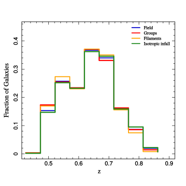
Figure 1: Normalised redshift distributions of the different samples of galaxies.

We identify filamentary structures that extend between groups of galaxies following Martínez et al. (2016). In what follows, unless otherwise specified, we make all computations using comoving distances in redshift space.

Firstly, we select candidates to be filaments nodes, which are pairs of groups ($i,j$) meeting the following criteria: 1) the projected distance (computed at the mean redshift) between them, $\Delta\pi_{ij}$, is smaller than a chosen value $\Delta\pi_{\text{max}}$, yet larger than the sum of their projected virial radii, $r^{(i)}_{\rm pv}+r^{(j)}_{\rm pv}<\Delta\pi_{ij}\leq\Delta\pi_{\rm max}$; 2) the line-of-sight distance between them, $\Delta\sigma_{ij}$, is smaller than certain $\Delta\sigma_{\rm max}$. The first condition ensures that the nodes are clearly separated structures in projection. In this work we use $\Delta\pi_{\rm max}=15~{}\rm{Mpc}$ and $\Delta\sigma_{\rm max}=15~{}\rm{Mpc}$.

Once groups $i$ and $j$ satisfy conditions 1) and 2) above, we use an overdensity criterion to decide whether there is a filament connecting them. We compute the galaxy overdensity in a rectangular cuboid with one of its axes aligned along the line-of-sight ($z-$axis), and whose base is in the plane of the sky with one of its sides parallel to the projected separation between the groups ($x-$axis), and the other perpendicular ($y-$axis). From the mean redshift of the pair, this rectangular cuboid extends $\pm 15~{}\rm{Mpc}$ alongside its $z-$axis. The base is positioned in order to cover the projected region between the two groups, while not overlapping with them (Fig. 1 of Martínez et al. 2016). Its dimensions are: $\Delta\pi_{ij}-r^{(i)}_{\rm pv}-r^{(j)}_{\rm pv}$ in the $x-$axis, and $\pm 1.5~{}\rm{Mpc}$ in the $y-$axis. The overdensity, $\delta=n/n_{r}-1$, is computed by counting VIPERS galaxies in this region ($n$), and points from a random catalogue that has the same angular mask and redshift distribution of VIPERS ($n_{r}$). Our random catalogue is $100$ times denser than VIPERS, thus we rescale $n_{r}$ accordingly. If $\delta>1$, we consider the pair is linked by a filament (Martínez et al., 2016). Out of 718 candidate pairs, we find 656 filaments.

3.3 Defining environments

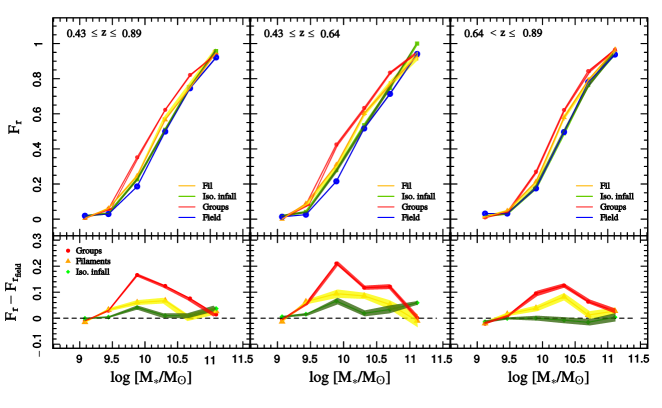
Figure 2: Red galaxies fraction as a function of stellar mass for our samples of galaxies. Left panel corresponds to the entire redshift range, central panel to the first redshift bin and the right panel to the high redshift bin. Colours denote environment: blue corresponds to field galaxies, green to isotropic infalling galaxies, dark yellow to galaxies in filaments, and red to galaxies in groups. Error-bars were computed with the bootstrap resampling technique.

The identification of filaments in VIPERS of the previous subsection determines three of our four subsamples which we use in our analyses below: galaxies in the groups that define the filaments (GG), galaxies in the filaments (FG), and galaxies in the infall regions of those groups that are not located in filaments (IG).

The sample of galaxies in groups (GG) is made of all VIPERS galaxies that were identified as members of the groups that are linked by filaments. This sample comprises 7407 galaxies.

The sample of galaxies in filaments (FG) includes all galaxies that were found to be in the filament regions identified in the previous subsection. Every FG is associated to its closest node. This means that each node in the filament defined by groups $i$ and $j$ contributes to the FG sample with galaxies that are as far as $\Delta\pi_{ij}/2$ in projection. Our sample of FG consists of 2311 galaxies.

We use the projected distance $\Delta\pi_{ij}/2$ to define the isotropic infall region around each group: a cylinder centred in the group and aligned along the line of sight direction, whose radius is $\Delta\pi_{ij}/2$, and whose height is $2\,\Delta\sigma_{\text{max}}$ (see Fig. 1 of Martínez et al. 2016). The isotropic infall sample amounts to 3931 galaxies.

Nodes can be one of the extreme point of more than one filament, thus they may contribute to both, FG and IG samples, more than once and up to different projected distances. We check the samples in order not to have repeated galaxies. By construction, the GG, FG and IG samples have similar redshift distributions, as can be seen in Fig. 1.

We also construct a sample of field galaxies (CG, C for control), by means of a Monte Carlo algorithm that randomly selects VIPERS galaxies in order to create a sample that has a similar redshift distribution as the previous three samples. We take special care of avoiding in the process all galaxies in groups, in filaments, and in the isotropic infall regions. Our CG sample comprises 30,299 galaxies. The normalised galaxy redshift distributions for the four environments probed are shown in Fig. 1.

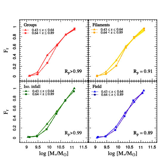
Figure 3: Passive galaxy fraction evolution. Top left panel shows galaxies in groups, Top rigth panel: galaxies in filaments, bottom left and right panel galaxies in the isotropic infall and field region, respectively. Solid lines correspond to the low-redshift bin, dashed lines to the high-redshift bin. Also, we show the results of applying the test of Muriel & Coenda (2014) (see text) to check whether the redshift evolution is statistically significant in each case.

4 RESULTS

	Rejection probability
Redshift range	FG vs. IG	FG vs. CG	IG vs. CG
$0.43\leq z\leq 0.64$	0.92	>0.99	>0.99
$0.64<z\leq 0.89$	0.96	>0.99	0.78

Table 1: Results of the test that computes the cumulative differences between the fractions of red galaxies of two different samples along the stellar mass domain (see Fig. 2). The quoted numbers are the rejection probability of the null hypothesis of two samples as drawn from the same underlying distribution.

We split our samples of galaxies into two redshift bins, defined by the median redshift $z_{\rm med}=0.64$, and then compute for each environment and redshift bin, the fraction of red galaxies as a function of stellar mass. These fractions can be seen in the upper panels of Fig. 2, where the left panel compares the four environments in the entire redshift range, the central does it at the first redshift bin ($0.43\leq z\leq 0.64$), and the right panel corresponds to the second redshift bin ($0.64<z\leq 0.89$). Lower panels in Fig. 2 show the differences in the fraction of quenched galaxies relative to the field values for a better visualization of the effects of the three densest environments we study. It should be remembered that, by construction, our samples of IG and FG are contaminated by field galaxies.

It is clear from Fig. 2 that stellar mass is the dominant factor behind galaxy quenching, as it has been extensively discussed in the literature (see for instance Peng et al. 2010). Independently of redshift and environment, the fraction of red (quenched) galaxies is a strong function of stellar mass.

In general, at the low mass end ($\log(M_{\star}/M_{\odot})\sim 9.1$), all environments appear to be ineffective to quench galaxies. On the contrary, at the highest mass bin ($\log(M_{\star}/M_{\odot})\sim 11.1$) all environment have a similar fraction of quenched galaxies, which indicates that galaxies this massive are likely to be quenched almost exclusively by internal processes. For masses in between those extremes, the differential effects of environment are evident at both redshift bins. As an overall trend, at fixed mass, GG have the highest fraction of quenched galaxies, followed by FG, and the lowest fraction is seen for field galaxies. The fraction of quenched galaxies in IG and CG are indistinguishable at our highest redshift bin. On the other hand, at our lowest redshift bin, the fraction of quenched IG and CG differ. With the former having an intermediate behavior between FG and CG.

Several authors (e.g. Sobral et al. 2011; Muzzin et al. 2012; Darvish et al. 2016) have presented evidence that the effects of environment upon galaxy quenching became noticeable by $z\sim 1$. The upper right panel of Fig. 2 shows evidence of environmental quenching by filaments already present at $0.64<z\leq 0.89$. The effects of the isotropic infall region became significant later on cosmic time, they are only present at our lowest redshift bin. This may be indicating that this environment was not dense enough at the highest redshift bin to produce any noticeable effect upon galaxies. This distinction between FG and IG, was reported at low redshift ($z\sim 0.1$) by Martínez et al. (2016).

We test whether differences seen in this figure are statistically significant by using a similar test to that of Muriel & Coenda (2014). When comparing two trends in Fig. 2, this test computes the cumulative differences between the fractions of red galaxies in the two samples along the stellar mass domain, and then checks whether the resulting quantity is consistent with the null hypothesis of the two samples drawn from the same underlying population. Results of the test for FG, IG and CG (GG are clearly different from these three) are quoted in Tab. 1 in terms of the rejection probability of null hypothesis ($R_{\rm p}$). This test confirms that the null hypothesis is overruled in all cases, with the exception of IG and CG at the highest redshift bin. The fact that the fraction of quenched IG and CG do not differ may be indicating that the isotropic infalling region around groups were an environment not different from the field at these redshift. On the other hand, filaments were already a distinctive environment at these times.

For a better visualization of redshift evolutions, all trends in Fig. 2 are re-arranged in Fig. 3, where we compare each environment with itself at the two redshift bins. In all four cases, there is clear evidence of an increment in the fraction of quenched galaxies with decreasing redshift. This evolution is seen for intermediate mass galaxies, $9.1\lesssim\log(M_{\star}/M_{\odot})\lesssim 10.4$, and is practically absent outside this range. For higher masses, all galaxies in all environments were already quenched at the high redshift bin; at the lowest mass bins there are almost no quenched galaxies at any of the two redshift bins. The latter means that galaxies with stellar masses $\log(M_{\star}/M_{\odot})\lesssim 9.1$ were difficult to quench at these times of the history of the Universe in the environments under consideration.

We quote in Fig. 3 the results of applying the test described above, to check whether the evolution of the fraction of red galaxies in each environment are statistically significant. In terms of of the rejection probability of null hypothesis, the fraction of red galaxies in GG at the two redshift bins are distinguible ($R_{\rm p}>0.99$), a similar result is found for the IG ($R_{\rm p}>0.99$), which supports the case for evolution in these two environments. The test is not that conclusive for FG ($R_{\rm p}=0.91$) nor for CG ($R_{\rm p}>0.89$).

There is another interesting feature in Fig. 3: the largest evolution in the fraction of quenched galaxies occurs at $\log(M_{\star}/M_{\odot})\sim 9.9$ irrespective of environment, with an almost null evolution for masses $\log(M_{\star}/M_{\odot})>10.3$. This evolution is stronger as we move from the field to higher density environments. This suggests that in the redshift range we probe, the galaxies that are the most likely to be quenched are those with mass $\log(M_{\star}/M_{\odot})\sim 9.9$. This should be due to a combination of internal and external factors. External factors are clearly present since the strength of the evolution depends on environment. On the other hand, the fact that, independently of environment, the largest change occurs at the same mass range, may be pointing out to these galaxies as the best prepared to be quenched, and this could be preferentially attributed to internal processes (mass quenching).

Another conclusion worth mentioning that can be deduced from our results is that galaxies that fell into groups at least as far back in time as $z\sim 0.9$, were likely to be pre-processed by the environment surrounding the systems. The likelihood of being pre-processed was higher if these galaxies happened to fell along filaments.

5 Summary

In this work we study the effects of environment on galaxy quenching at $0.43\leq z\leq 0.89$ using data from VIPERS. Firstly, we identify groups of galaxies and filamentary structures stretching between them. We study the fraction of passive galaxies (defined by their $NUV-r$ vs. $r-K$ colours) as a function of stellar mass in 4 different environments: field, filaments, the isotropic infalling region of groups, and groups. We also studied, for each environment, the evolution of the fraction of quenched galaxies within the redshift range covered by VIPERS.

The effects of environment are significant for intermediate mass galaxies: the fraction of quenched galaxies is lowest in the field, higher in the isotropic infall region, even higher in filaments, and finally the highest values are reached in groups. At the two extremes in stellar mass, we found opposite situations: on the one hand, massive galaxies do not appear to require the action of environment to be quenched; on the other hand, the least massive galaxies in our samples, are hardly affected by the environment at all.

We find evidence of environmental quenching in galaxies in filaments at least from $z\sim 0.9$, and in the isotropic infall region of groups from $z\sim 0.6$ onwards. There is evolution in the fraction of intermediate mass galaxies in the redshift range under study. This evolution is stronger in groups, followed by filaments, the isotropic infall region, and the mildest (if any) evolution is seen in the field.

References

- Abazajian et al. (2009) Abazajian K. N., et al., 2009, ApJS, 182, 543
- Alpaslan et al. (2014) Alpaslan M., et al., 2014, MNRAS, 440, L106
- Alpaslan et al. (2015) Alpaslan M., et al., 2015, MNRAS, 451, 3249
- Alpaslan et al. (2016) Alpaslan M., et al., 2016, MNRAS, 457, 2287
- Aragón-Calvo et al. (2007) Aragón-Calvo M. A., Jones B. J. T., van de Weygaert R., van der Hulst J. M., 2007, A&A, 474, 315
- Aragón-Calvo et al. (2010) Aragón-Calvo M. A., van de Weygaert R., Jones B. J. T., 2010, MNRAS, 408, 2163
- Arnouts et al. (2013) Arnouts S., et al., 2013, A&A, 558, A67
- Barrow et al. (1985) Barrow J. D., Bhavsar S. P., Sonoda D. H., 1985, MNRAS, 216, 17
- Beers et al. (1990) Beers T. C., Flynn K., Gebhardt K., 1990, AJ, 100, 32
- Bolzonella et al. (2000) Bolzonella M., Miralles J.-M., Pelló R., 2000, A&A, 363, 476
- Bond et al. (1996) Bond J. R., Kofman L., Pogosyan D., 1996, Nature, 380, 603
- Bruzual & Charlot (2003) Bruzual G., Charlot S., 2003, MNRAS, 344, 1000
- Calzetti et al. (2000) Calzetti D., Armus L., Bohlin R. C., Kinney A. L., Koornneef J., Storchi-Bergmann T., 2000, ApJ, 533, 682
- Cautun et al. (2013) Cautun M., van de Weygaert R., Jones B. J. T., 2013, MNRAS, 429, 1286
- Cautun et al. (2014) Cautun M., van de Weygaert R., Jones B. J. T., Frenk C. S., 2014, MNRAS, 441, 2923
- Chabrier (2003) Chabrier G., 2003, PASP, 115, 763
- Chen et al. (2017) Chen Y.-C., et al., 2017, MNRAS, 466, 1880
- Coenda et al. (2018) Coenda V., Martínez H. J., Muriel H., 2018, MNRAS, 473, 5617
- Colberg (2007) Colberg J. M., 2007, MNRAS, 375, 337
- Cucciati et al. (2017) Cucciati O., et al., 2017, A&A, 602, A15
- Darvish et al. (2014) Darvish B., Sobral D., Mobasher B., Scoville N. Z., Best P., Sales L. V., Smail I., 2014, ApJ, 796, 51
- Darvish et al. (2016) Darvish B., Mobasher B., Sobral D., Rettura A., Scoville N., Faisst A., Capak P., 2016, ApJ, 825, 113
- Davidzon et al. (2016) Davidzon I., et al., 2016, A&A, 586, A23
- Dressler (1980) Dressler A., 1980, ApJ, 236, 351
- Driver et al. (2009) Driver S. P., et al., 2009, Astronomy and Geophysics, 50, 5.12
- Eardley et al. (2015) Eardley E., et al., 2015, MNRAS, 448, 3665
- Eke et al. (2004) Eke V. R., et al., 2004, MNRAS, 348, 866
- Fritz et al. (2014) Fritz A., et al., 2014, A&A, 563, A92
- Garilli et al. (2014) Garilli B., et al., 2014, A&A, 562, A23
- Gómez et al. (2003) Gómez P. L., et al., 2003, ApJ, 584, 210
- Guzzo et al. (2014) Guzzo L., et al., 2014, A&A, 566, A108
- Huchra & Geller (1982) Huchra J. P., Geller M. J., 1982, ApJ, 257, 423
- Just et al. (2015) Just D. W., et al., 2015, preprint, (arXiv:1506.02051)
- Knobel et al. (2012) Knobel C., et al., 2012, ApJ, 753, 121
- Kovač et al. (2010) Kovač K., et al., 2010, ApJ, 718, 86
- Kraljic et al. (2018) Kraljic K., et al., 2018, MNRAS, 474, 547
- Laigle et al. (2018) Laigle C., et al., 2018, MNRAS, 474, 5437
- Le Févre et al. (2003) Le Févre O., et al., 2003, MNRAS, 4841, 1670
- Lilly et al. (2007) Lilly S. J., et al., 2007, ApJS, 172, 70
- Malavasi et al. (2017) Malavasi N., et al., 2017, MNRAS, 465, 3817
- Martin et al. (2005) Martin D. C., et al., 2005, ApJ, 619, L1
- Martínez & Muriel (2006) Martínez H. J., Muriel H., 2006, MNRAS, 370, 1003
- Martínez et al. (2008) Martínez H. J., Coenda V., Muriel H., 2008, MNRAS, 391, 585
- Martínez et al. (2016) Martínez H. J., Muriel H., Coenda V., 2016, MNRAS, 455, 127
- Moutard et al. (2016) Moutard T., et al., 2016, A&A, 590, A102
- Muriel & Coenda (2014) Muriel H., Coenda V., 2014, A&A, 564, A85
- Muzzin et al. (2012) Muzzin A., et al., 2012, ApJ, 746, 188
- Novikov et al. (2006) Novikov D., Colombi S., Doré O., 2006, MNRAS, 366, 1201
- Peng et al. (2010) Peng Y.-j., et al., 2010, ApJ, 721, 193
- Pimbblet (2005) Pimbblet K. A., 2005, MNRAS, 358, 256
- Presotto et al. (2012) Presotto V., et al., 2012, A&A, 539, A55
- Puget et al. (2004) Puget P., et al., 2004, in Moorwood A. F. M., Iye M., eds, Proc. SPIEVol. 5492, Ground-based Instrumentation for Astronomy. pp 978–987, doi:10.1117/12.551097
- Scodeggio et al. (2018) Scodeggio M., et al., 2018, A&A, 609, A84
- Scoville et al. (2007) Scoville N., et al., 2007, ApJS, 172, 38
- Sobral et al. (2011) Sobral D., Best P. N., Smail I., Geach J. E., Cirasuolo M., Garn T., Dalton G. B., 2011, MNRAS, 411, 675
- Sousbie (2011) Sousbie T., 2011, MNRAS, 414, 350
- White et al. (2005) White S. D. M., et al., 2005, A&A, 444, 365
- Wilman et al. (2009) Wilman D. J., Oemler Jr. A., Mulchaey J. S., McGee S. L., Balogh M. L., Bower R. G., 2009, ApJ, 692, 298
- Zhang et al. (2013) Zhang Y., Dietrich J. P., McKay T. A., Sheldon E. S., Nguyen A. T. Q., 2013, ApJ, 773, 115