Removing instabilities in the hierarchical equations of motion: exact and approximate projection approaches

Abstract

The hierarchical equations of motion (HEOM) provide a numerically exact approach for computing the reduced dynamics of a quantum system linearly coupled to a bath. We have found that HEOM contains temperature-dependent instabilities that grow exponentially in time. In the case of continuous-bath models, these instabilities may be delayed to later times by increasing the hierarchy dimension; however, for systems coupled to discrete, non-dispersive modes, increasing the hierarchy dimension does little to alleviate the problem. We show that these instabilities can also be removed completely at a potentially much lower cost via projection onto the space of stable eigenmodes; furthermore, we find that for discrete-bath models at zero temperature, the remaining projected dynamics computed with few hierarchy levels are essentially identical to the exact dynamics that otherwise might require an intractably large number of hierarchy levels for convergence. Recognizing that computation of the eigenmodes might be prohibitive, e.g. for large or strongly-coupled models, we present a Prony filtration algorithm that may be useful as an alternative for accomplishing this projection when diagonalization is too costly. We present results demonstrating the efficacy of HEOM projected via diagonalization and Prony filtration. We also discuss issues associated with the nonnormality of HEOM.

I Introduction

A grand challenge in the physical sciences lies in modeling quantum dynamics in the condensed phase(Berne et al., 1998; May and Kühn, 2011; Weiss, 2012; Nitzan, 2006). Progress has often been made by using efficient approximate approaches that invoke a “system-bath” separation and treat the bath classically(Billing, 1975; Chen and Reichman, 2016) or the system-bath interactions perturbatively(Redfield, 1965). However, in systems where quantum effects in the bath play a pronounced role and where no small coupling or energy parameter may be identified, exact solutions to a fully quantum system-bath model are desired. One of the most successful computational methods for calculating exact quantum dynamics is provided by the hierarchical equations of motion (HEOM)(Tanimura and Kubo, 1989; Ishizaki and Tanimura, 2005; Ishizaki and Fleming, 2009; Chen et al., 2009; Tanimura, 2014). First derived by Tanimura and Kubo(Tanimura and Kubo, 1989), HEOM is a reformulation of the Feynman-Vernon influence functional approach to quantum dissipative dynamics(Feynman and Vernon, 1963; Tanimura and Kubo, 1989; Makri and Makarov, 1995a, b; Ishizaki and Tanimura, 2005; Ishizaki and Fleming, 2009; Liu et al., 2014; Chen et al., 2015), and its solution yields the exact reduced dynamics of linearly coupled system-bath models. HEOM has successfully addressed a variety of applications; yet, its scope is limited since the original formulation of HEOM requires the bath to be represented by a continuous spectral density. Such a constraint is often inappropriate for describing phenomena captured in venerable models of quasi-particle dynamics in organic molecular crystals(Spano, 2010; Bakulin et al., 2016; Tempelaar and Reichman, 2018; Fujihashi et al., 2017; Morrison and Herbert, 2017), coupled excitonic and vibrational motion in light harvesting complexes(Womick and Moran, 2011; Christensson et al., 2012; Tiwari et al., 2013; Tempelaar et al., 2014), and transport in polar crystals with narrow phonon bandwidths(Fröhlich, 1954; Feynman, 1955; Feynman et al., 1962; Devreese and Alexandrov, 2009). In these cases where discrete bath modes play a significant role, efficient and exact methods for computing quantum dynamics are desirable.

Motivated by the aforementioned computational challenges, several groups have recently explored novel formulations of HEOM that treat a discrete spectral density(Liu et al., 2014; Chen et al., 2015). There are several potential advantages in developing a “discrete-bath HEOM”. First, even in the discrete-bath formulation, HEOM retains the benefit that the reduced equations automatically include all possible bath excitations. As a result, HEOM eliminates the issue of basis-set convergence present in techniques such as exact diagonalization and matrix product states, and instead relies on convergence with respect to hierarchy depth (number of hierarchy levels, see II.2). Second, including discrete bath modes in HEOM serves to expand the ability of this powerful methodology to tackle an important class of problems, with the added benefit that several popular HEOM software packages such as Parallel Hierarchy Integrator(Strümpfer and Schulten, 2012) (PHI), pyrho(Berkelbach, ), and potentially also GPU-HEOM(Kreisbeck et al., 2011) can be readily adapted for the discrete-bath case.

Figure 1: Time evolution of electron density for a 10-site periodic Holstein model with a dispersive phonon band (as defined in eqs. 1-4 of Chen et al.(Chen et al., 2015)) calculated via HEOM with 5 hierarchy levels. $P_{n}(t)\equiv\langle a_{n}^{\dagger}(t)a_{n}(t)\rangle$. Model parameters: $g=0.1,\omega_{0}=1,W=0.5,J=0.2,T=0$. This is an extension to longer times of the simulation performed in Fig. 1a of Chen et al., which was originally run to time $12\pi/\omega_{0}$(Chen et al., 2015). Calculations were performed using a modified version of PHI(Strümpfer and Schulten, 2012).

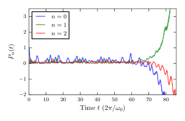
Nonetheless, existing formulations of discrete-bath HEOM are not without serious problems that we will explore and partially remedy in this work. Recently, Chen et al.(Chen et al., 2015) published discrete-bath HEOM simulations which converge with few hierarchy levels to the exact reduced dynamics for a 10-site Holstein model. We find that upon extending the time of these simulations, the dynamics are eventually plagued by the abrupt onset of an exponential instability. This instability is illustrated in Fig. 1. Unfortunately, increasing the number of hierarchy levels does little to delay this instability to later times and comes with a great computational cost. In the interest of honing HEOM to be a useful tool for modeling the dynamics of discrete-bath models, in this work we explore such instabilities and discuss approaches for removing them to facilitate longer-time simulations without the need for a large hierarchy depth. We also show that similar instabilities exist in the original “continuous-bath HEOM” at low temperatures. Our main finding, which is explicit in the discrete-bath case and plausible in the continuous-bath case, is that one can remove these instabilities without altering the exact long-time dynamics.

In this work we proceed as follows. In II we introduce the condensed phase models which we study, as well as the HEOM that describe their dynamics. In III we introduce our spectral approach for studying the stability of HEOM and illustrate several stable and unstable examples. In IV, we then apply our stability analysis to both discrete-bath and continuous-bath HEOM at nonzero temperatures, providing a brief discussion of instabilities in low-temperature continuous-bath HEOM that has only been alluded to(Moix and Cao, 2013) in the vast HEOM literature. In V we discuss a diagonalization approach for exactly projecting out the instabilities in discrete-bath HEOM. In VI we present an iterative method for accomplishing this projection that does not require the full diagonalization of the HEOM. Finally, in VII we comment on some difficulties that may arise due to the nonnormality of HEOM.

II Theory

II.1 Model Hamiltonians

To demonstrate instabilities in HEOM we consider several standard system-bath models for open quantum dynamics. Each of these models takes the form

$$\hat{H} =\hat{H}_{s}+\hat{H}_{b}+\hat{H}_{sb},$$ (1)

where $\hat{H}_{s}$ describes the degrees of freedom (DOFs) of the reduced system, $\hat{H}_{b}$ describes the DOFs of the phonon bath, and $\hat{H}_{sb}$ describes the coupling between the system and bath DOFs. In following sections, we will refer to the delta-function spin-boson model (DSB), the Holstein model(Holstein, 1959a, b), and the Su-Schrieffer-Heeger (SSH) model(Su et al., 1979) as discrete-bath models. Likewise, we will refer to the continuous spin-boson model (CSB) as a continuous-bath model. $\hat{a}$ and $\hat{b}$ are electron and phonon annihilation operators, respectively. We work in dimensionless units and set $\hbar=1$.

II.1.1 Spin-Boson Model

In this work, we consider a spin-boson model(Weiss, 2012; Chen and Reichman, 2016) with no energy bias between sites. The system has two energy levels,

$$\hat{H}_{s} =-J\left(\hat{a}_{1}^{\dagger}\hat{a}_{0}+\hat{a}_{0}^{\dagger}\hat{a}_{1}\right),$$ (2)

where $J$ is the inter-site coupling constant. This two-level system interacts with a harmonic oscillator bath

$$\hat{H}_{b} =\sum_{j=1}^{N_{b}}\omega_{j}\hat{b}_{j}^{\dagger}\hat{b}_{j},$$ (3)

where $\omega_{j}$ is the frequency of the $j$-th bath mode. We consider two forms of this model. In the DSB there is only one bath oscillator, such that $N_{b}=1$, $\omega_{j}\equiv\omega_{0}$, and $b_{j}\equiv b$. For the DSB, the coupling is defined as

$$\hat{H}_{sb} =-g\omega_{0}\hat{V}\left(\hat{b}+\hat{b}^{\dagger}\right),$$ (4)

where

$$\hat{V} =\hat{a}_{0}^{\dagger}\hat{a}_{0}-\hat{a}_{1}^{\dagger}\hat{a}_{1}.$$ (5)

In the CSB an infinite number of bath oscillators are included. For the CSB, the coupling is defined as

$$\hat{H}_{sb} =-\hat{V}\sum_{j=1}^{N_{b}}c_{j}\left(\hat{b}_{j}+\hat{b}_{j}^{\dagger}\right),$$ (6)

where

$$\hat{V} =\hat{a}_{0}^{\dagger}\hat{a}_{0}-\hat{a}_{1}^{\dagger}\hat{a}_{1}.$$ (7)

The coefficients $c_{j}$ are fixed via the spectral density

$$J(\omega) =\sum_{j=1}^{N_{b}}c_{j}^{2}\delta\left(\omega-\omega_{j}\right),$$ (8)

which we choose in this work to be the Debye spectral density

$$J(\omega) =\frac{2}{\pi}\frac{\lambda\gamma\omega}{\omega^{2}+\gamma^{2}}.$$ (9)

In practice, the spin-boson model may be used as a coarse-grained description for any system that is well approximated by a two-level system coupled linearly to a harmonic bath. Applications of the spin-boson model are enumerated by Weiss and include the description of qubits, tunneling phenomena, and electron transfer processes(Weiss, 2012).

II.1.2 Holstein model

We also consider a one-dimensional Holstein model(Holstein, 1959a, b; Mahan, 2000) with periodic boundary conditions. The system is described by a tight-binding Hamiltonian

$$\hat{H}_{s} =-J\sum_{n=1}^{N}\hat{a}_{n}^{\dagger}\left(\hat{a}_{n+1}+\hat{a}_{n-1}\right),$$ (10)

interacting with a harmonic oscillator bath

$$\hat{H}_{b} =\omega_{0}\sum_{n=1}^{N}\hat{b}_{n}^{\dagger}\hat{b}_{n},$$ (11)

with site-diagonal coupling

$$\hat{H}_{sb} =-g\omega_{0}\sum_{n=1}^{N}\hat{V}_{n}\left(\hat{b}_{n}+\hat{b}_{n}^{\dagger}\right),$$ (12)

where

$$\hat{V}_{n} =\hat{a}_{n}^{\dagger}\hat{a}_{n}.$$ (13)

The Holstein model, termed a “molecular crystal model,” was introduced to extend the conventional continuum treatment of polarons(Pekar, 1946; Fröhlich, 1954) to account for the deformation of a discrete lattice(Holstein, 1959a, b). It reflects the decoupled nature of sites in a molecular crystal by including only local electron-phonon coupling under the assumption of Einstein phonons. The Holstein model has the advantage that it can be used for a range of coupling strengths to describe large and small polarons, alike(Holstein, 1959a, b). For an excellent review that discusses the relation between the Holstein model and the Fröhlich model as well as the DSB, see Devreese and Alexandrov(Devreese and Alexandrov, 2009). In addition to modeling electron dynamics, the Holstein model has also seen great success in modeling Frenkel exciton dynamics in organic molecular crystals(Merrifield, 1964; Spano, 2010; Hestand and Spano, 2018).

II.1.3 Su-Schrieffer-Heeger model (SSH)

As an alternative to the Holstein model, we also briefly consider the SSH model(Su et al., 1979) with periodic boundary conditions, which differs from the Holstein model in its off-diagonal system-bath coupling

$$\hat{H}_{sb} =-gJ\sum_{n=1}^{N}\hat{V}_{n}\left[\left(\hat{b}_{n}+\hat{b}_{n}^{\dagger}\right)-\left(\hat{b}_{n+1}+\hat{b}_{n+1}^{\dagger}\right)\right],$$ (14)

where

$$\hat{V}_{n} =\hat{a}_{n}^{\dagger}\hat{a}_{n+1}+\hat{a}_{n+1}^{\dagger}\hat{a}_{n}.$$ (15)

The SSH model was originally proposed to describe solitons in polyacetylene(Su et al., 1979), and has also been employed to model charge transport in crystalline organic semiconductors(De Filippis et al., 2015). The SSH coupling (14) accounts for the modulation of electron-hopping rates based on the variable nuclear distance between sites. When the SSH coupling (14) is combined with the Holstein coupling (12), the resulting model which includes both local deformation and phonon-mediated hopping is known as the Holstein-Peierls model(Munn and Silbey, 1985).

II.2 The hierarchical equations of motion

We now formally define HEOM, the exact quantum dynamics method of interest in this work. HEOM consists of a set of coupled linear differential equations that govern the time evolution of a hierarchy of indexed matrices. At the root of the hierarchy lies the reduced density matrix of the system,

$$\hat{\sigma}(t) =\hat{\rho}_{0,..,0}(t).$$ (16)

The dynamics of the DSB, Holstein model, and SSH model are described by the following HEOM(Liu et al., 2014; Chen et al., 2015).

$$\frac{d}{dt}\hat{\rho}_{m_{1\pm},...,m_{N_{b}\pm}}(t) =-i\mathcal{L}\hat{\rho}_{m_{1\pm},...,m_{N_{b}\pm}}(t)$$

$$-i\sum_{n=1}^{N_{b}}\omega_{0}\left(m_{n-}-m_{n+}\right)\hat{\rho}_{m_{1\pm},...,m_{N_{b}\pm}}(t)$$

$$+\sum_{n=1}^{N_{b}}\biggr{[}\Phi_{n}\biggr{(}\hat{\rho}_{m_{1\pm},...,m_{n+}+1,...,m_{N_{b}\pm}}(t)$$

$$+\hat{\rho}_{m_{1\pm},...,m_{n-}+1,...,m_{N_{b}\pm}}(t)\biggr{)}$$

$$+m_{n+}\Theta_{n+}\hat{\rho}_{m_{1\pm},...,m_{n+}-1,...,m_{N_{b}\pm}}(t)$$

$$+m_{n-}\Theta_{n-}\hat{\rho}_{m_{1\pm},...,m_{n-}-1,...,m_{N_{b}\pm}}(t)\biggr{]},$$ (17)

where

$$\mathcal{L} =[\hat{H}_{s},...],$$ (18)

and

$$\Phi_{n} =[\hat{V}_{n},...].$$ (19)

For the Holstein model and the DSB,

$$\Theta_{n\pm} =-\frac{\left(g\omega_{0}\right)^{2}}{2}\left([\hat{V}_{n},...]\coth\left(\frac{\beta\omega_{0}}{2}\right)\mp\{\hat{V}_{n},...\}\right),$$ (20)

while for the SSH model

$$\Theta_{n\pm} =-\frac{\left(gJ\right)^{2}}{2}\biggr{(}[\hat{V}_{n}-\hat{V}_{n-1},...]\coth\left(\frac{\beta\omega_{0}}{2}\right)$$

$$\mp\{\hat{V}_{n}-\hat{V}_{n-1},...\}\biggr{)}.$$ (21)

For the Holstein and SSH models, $N_{b}=N$. For the DSB, $N_{b}=1$ and $\hat{V}_{n}=\hat{V}$. Throughout this paper we define the inverse temperature $\beta=\left(k_{B}T\right)^{-1}$ and work in units where $k_{B}=1$.

The $l$-th hierarchy level consists of all matrices $\hat{\rho}_{m_{1\pm},...,m_{N_{b}\pm}}(t)$ in Eq. (17) for which

$$\sum_{n+=1}^{N_{b}}m_{n+}+\sum_{n-=1}^{N_{b}}m_{n-} =l.$$ (22)

In this study we truncate this infinite hierarchy of coupled differential equations after $L$ hierarchy levels with a “time-nonlocal” closure(Chen et al., 2009; Liu et al., 2014; Chen et al., 2015), where we set

$$\hat{\rho}_{m_{1\pm},...,m_{N_{b}\pm}}(t) =0$$ (23)

for

$$\sum_{n+=1}^{N_{b}}m_{n+}+\sum_{n-=1}^{N_{b}}m_{n-} \geq L.$$ (24)

In practice, solutions to (17) are to be converged with respect to the hierarchy depth $L$.

The CSB is described by the following HEOM(Ishizaki and Tanimura, 2005), which are similar in structure to Eq. (17) but produce markedly different dynamics due to the incorporation of an infinite bath.

$$\frac{d}{dt}\hat{\rho}_{m_{0},...,m_{K}}(t) =\left[-i\mathcal{L}-\sum_{k=0}^{K}m_{k}\nu_{k}\right]\hat{\rho}_{m_{0},...,m_{K}}(t)$$

$$+\sum_{k=0}^{K}\biggr{[}\Phi\hat{\rho}_{m_{0},...,m_{k}+1,...,m_{K}}(t)$$

$$+\sum_{k=0}^{K}m_{k}\Theta_{k}\hat{\rho}_{m_{0},...,m_{k}-1,...,m_{K}}(t)\biggr{]},$$ (25)

where

$$\mathcal{L} =[\hat{H}_{s},...],$$ (26)

$$\Phi =[\hat{V},...],$$ (27)

$$\Theta_{0} =-\lambda\gamma\left(\cot\left(\frac{\beta\gamma}{2}\right)[\hat{V},...]-i\{\hat{V},...\}\right),$$ (28)

$$\Theta_{k\neq 0} =-\frac{4\lambda\gamma\nu_{k}}{\beta}\frac{1}{\nu_{k}^{2}-\gamma^{2}}[\hat{V},...],$$ (29)

$$\nu_{0} =\gamma,$$ (30)

and

$$\nu_{k\neq 0} =\frac{2\pi k}{\beta}.$$ (31)

Eq. (25) incorporates an infinite Matsubara series, resulting from a high-temperature expansion, that is closed via truncation after $K$ Matsubara terms. Another popular closure for the Matsubara series in HEOM was derived by Ishizaki and Tanimura(Ishizaki and Tanimura, 2005). The Ishizaki-Tanimura closure approximately accounts for Matsubara terms with $k>K$ (for sufficiently large $K$) by replacing rapidly decaying factors of $\nu_{k}e^{-\nu_{k}t}$ with $\delta\left(t\right)$; this closure also has the added benefit of improved stability, although instabilities are still present. However, in the interest of using a continuous-bath HEOM that closely resembles the discrete-bath formulation in Eq. (17) we will not employ the Ishizaki-Tanimura closure in this work.

Here, the $l$-th hierarchy level consists of all matrices $\hat{\rho}_{m_{0},...,m_{K}}(t)$ in Eq. (17) for which

$$\sum_{k=0}^{K}m_{k} =l.$$ (32)

Again, we use a time-nonlocal closure after $L$ hierarchy levels(Ishizaki and Tanimura, 2005; Chen et al., 2009) such that

$$\hat{\rho}_{m_{0},...,m_{K}}(t) =0$$ (33)

for

$$\sum_{k=0}^{K}m_{k} \geq L.$$ (34)

In practice, solutions to (25) are to be converged with respect to the hierarchy depth $L$, as well as the number of Matsubara terms $K$.

Alternate closures exist for Eqs. (17) and (25) besides those shown in Eqs. (24) and (34). Continuous-bath HEOM studies regularly employ a closure that relies on the exponential suppression of deeper hierarchy levels(Tanimura and Wolynes, 1991; Ishizaki and Tanimura, 2005); we do not investigate this closure here since it is not applicable to discrete-bath models. Furthermore, the time-local closure(Xu et al., 2005; Chen et al., 2009) is applicable for both discrete-bath HEOM and continuous-bath HEOM; however, since it does not appear to suppress instabilities in discrete-bath HEOM and also is not amenable to the spectral analysis in III, we do not explore the time-local closure here.

For the initial condition employed in this work, similar to many other studies, we set the population of the first site $\rho_{0,...,0}^{00}(t=0)=1$, and all the other hierarchical matrix elements are set to zero.

III Spectral analysis

The HEOM presented in Eqs. (17) and (25) may be represented as linear systems of the form

$$\frac{d}{dt}\vec{\rho}(t) =A\vec{\rho}(t),$$ (35)

where $\vec{\rho}(t)$ is a vector containing all the hierarchy elements $\rho_{m_{1\pm},...,m_{N_{b}\pm}}^{ij}(t)$ or $\rho_{m_{0},...,m_{K}}^{ij}(t)$ and $A$ is a nonnormal matrix containing the coupling between all of the hierarchy elements. With this flattened representation of HEOM, spectral analysis can be used to study the stability of solutions. The solution to Eq. (35) may be written as

$$\vec{\rho}(t) =e^{At}\vec{\rho}(0).$$ (36)

Assuming $A$ to be a diagonalizable matrix and employing the eigen-decomposition of $A$, we can write Eq. (36) as

$$\vec{\rho}(t) =Ve^{\Lambda t}V^{-1}\vec{\rho}(0),$$ (37)

where $\Lambda$ is a diagonal matrix containing the eigenvalues $\{\lambda_{i}\}$ of $A$ and $V$ is a matrix whose columns $\vec{v}_{i}$ are the normalized eigenvectors of $A$. We can write Eq. (37) in the eigenbasis of $A$ as

$$\vec{\rho}(t) =\sum_{i}d_{i}e^{\lambda_{i}t}\vec{v}_{i},$$ (38)

where the components of $\vec{d}=V^{-1}\vec{\rho}(0)$ are the expansion coefficients of $\vec{\rho}(0)$ in the eigenbasis of $A$. From this representation, it is clear that terms in the sum with $\Re[\lambda_{i}]>0$ are asymptotically unstable, and will be referred to here as the unstable modes.

Figure 2: Spectrum of $A$ for a 2-site Holstein model at $T=0$ with $L=9$. Model parameters: $g=0.5,\omega_{0}=1,J=0.2$.

III.1 Unstable HEOM

Figure 3: Spectrum of $A$ for a 3-site SSH model at $T=0$ with $L=5$. Model parameters: $g=0.5,\omega_{0}=1,J=0.2$.

Figure 4: Spectrum of $A$ for the CSB with $L=20,K=0$. Model parameters: $\sqrt{\lambda}=0.3,\gamma=1,J=0.2,T=0.16$.

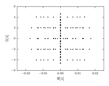
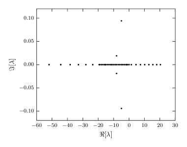
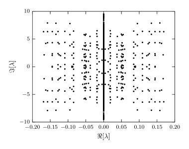
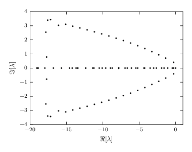
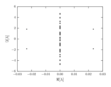
In Fig. 2 and Fig. 3 we calculate the eigen-decomposition for the flattened representation of Eq. (17) and plot $\{\lambda_{i}\}$ for two discrete-bath models: the 2-site Holstein model and the 3-site SSH model. Likewise, in Fig. 4 we do the same for the CSB described by Eq. (25). Notice that eigenvalues are present in the right half-plane in all three cases: these eigenvalues correspond to unstable modes. Furthermore, computing $\vec{d}$, the decomposition of $\vec{\rho}(0)$ in the eigenbasis of $A$, reveals that some of these unstable modes have nonzero weights in the initial condition, leading to asymptotic instability in the dynamics. In the following sections we will interpret these unstable modes and discuss computational strategies for removing them.

While we have shown in Fig. 4 a particularly unstable example of continuous-bath HEOM, in many practical continuous-bath cases one can suppress any instabilities by converging with respect to $L$ and $K$ and employing the Ishizaki-Tanimura closure(Ishizaki and Tanimura, 2005) for the Matsubara series. To the contrary, instabilities are much harder to suppress via convergence with respect to $L$ in discrete-bath HEOM.

III.2 Asymptotically Stable HEOM

To show an example of asymptotically stable HEOM, we will now contrast the former unstable examples with the HEOM for the CSB (25) at a temperature where no unstable modes are present. In Fig. 5 we again show the spectrum of the flattened representation of Eq. (25)

Figure 5: Spectrum of $A$ for the CSB with $L=20,K=0.$ Model parameters: $\sqrt{\lambda}=0.5,\gamma=1,J=0.2,T=0.4$.

(the HEOM for the CSB), only this time at a higher temperature. Since the high-temperature $K=0$ approximation for continuous-bath HEOM is known to be equivalent to the Zusman equation(Shi et al., 2009), we note the resemblance here to the eigentree structure from the Zusman equation spectral analysis reported by Jung et al.(Jung et al., 1999). It is clear that all eigenvalues are confined to the left half-plane of Fig. 5. As a result, the corresponding dynamics are asymptotically stable.

At this point, we would be remiss to not acknowledge the structure and symmetry present in the spectral plots of Figs. 2, 3, 4, and 5. While we omit a discussion of the spectral dependence on hierarchy depth, number of sites, and choice of model, we exemplify these dependences in the animations shown in the supplementary material.

IV Temperature Dependence of HEOM Spectra

The spectra of both discrete-bath HEOM and continuous-bath HEOM admit a rich temperature dependence. In Figs. 6, 7, and 8

Figure 6: Real part of most unstable eigenvalue for the DSB, plotted as a function of temperature for a range of hierarchy depths. Model parameters: $g=0.4,\omega_{0}=1,J=0.2$.

Figure 7: Real part of most unstable eigenvalue for the CSB, plotted as a function of temperature for a variety of Matsubara dimensions. Model parameters: $\sqrt{\lambda}=0.8,\gamma=1,J=0.2$. $L=3$.

Figure 8: Real part of most unstable eigenvalue for the CSB, plotted as a function of temperature for a variety of hierarchy depths. Model parameters: $\sqrt{\lambda}=0.8,\gamma=1,J=0.2$. $K=0$.

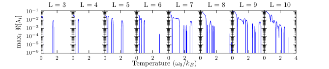
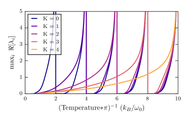
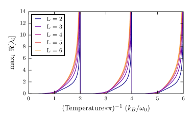
we plot for the DSB and the CSB the real part of the most unstable eigenvalue, $\max_{i}\Re\left[\lambda_{i}\right]$, as a function of temperature. Note the similarity between the qualitative behavior in Fig. 6 and Figs. 7 and 8. Both discrete-bath and continuous-bath HEOM reveal unstable regions, i.e. temperature ranges where $\max_{i}\Re\left[\lambda_{i}\right]>0$, intermingled with stable regions. Furthermore, both have unstable regions concentrated at lower temperatures.

While there are gross similarities between these cases, there are several important differences of note. First, the behavior shown in Fig. 6 seems to be piecewise continuous while that of Figs. 7 and 8 contains many asymptotes. A simple analytically solvable example that helps us rationalize the appearance of these asymptotes for the CSB will be discussed in the Appendix. Second, while the discrete-bath HEOM instabilities in Fig. 6 are governed by a single convergence parameter $L$, the behavior appears quite complicated: note how the unstable regions merge at lower temperatures and tend to grow more unstable as $L$ is increased. Since the unstable regions shift as a function of hierarchy depth, the behavior of the HEOM solution may be erratic as the hierarchy depth is varied for a fixed temperature, since instabilities may appear and disappear and vary in severity at any fixed temperature. In contrast, for continuous-bath HEOM we see two distinct types of behavior governed by the parameters $K$ and $L$. In Fig. 7 we see that as $K$ is incremented, unstable asymptotes are annihilated one at a time without changing the temperatures of the remaining asymptotes, effectively lowering the upper bound on temperatures at which instabilities become problematic. In Fig. 8 we observe that as $L$ increases, the unstable regions simply change in shape and the temperatures at which asymptotes occur are invariant. Thus, we find that for continuous-bath HEOM $K$ is predominantly responsible for controlling the most severe instabilities; an increase in $L$ alone cannot remove the instability.

Next, we turn to the low-temperature behavior in continuous-bath and discrete-bath HEOM as it relates to the aforementioned instabilities. In continuous-bath HEOM, low temperatures are manifestly problematic since the HEOM are derived using a high-temperature Matsubara expansion. At $T=0$ continuous-bath HEOM as expressed in Eq. (25) is ill-defined due to the explicit factor of $\cot\left(\beta\gamma/2\right)$ that appears in Eq. 28. For small non-zero temperatures the situation is still problematic; while the HEOM are defined at temperatures between the asymptotes of $\cot\left(\beta\gamma/2\right)$, due to the high density of asymptotes (per unit temperature) at low temperature it is necessary to use a large $K$ to annihilate the offending asymptotes and obtain converged dynamics. The situation is quite different in discrete-bath HEOM, where there is no high-temperature expansion and no notion of Matsubara convergence. It would seem therefore that discrete-bath HEOM should be amenable to facile low temperatures simulations as claimed by Chen et al.(Chen et al., 2015). While the discrete-bath HEOM are indeed well-defined at all temperatures, they do not eliminate the issue of instabilities at low temperature. Specifically, the low-temperature instability that in continuous-bath HEOM is controlled by the number of Matsubara terms reappears in discrete-bath HEOM as an instability that is controlled by the hierarchy depth. Now that we have investigated the temperature-dependence of the instabilities, we focus our attention on methods for overcoming instabilities in discrete-bath HEOM at $T=0$.

V Projecting away instabilities exactly

Let us momentarily abandon the goal of extracting a physical $\vec{\rho}(t)$ from the unstable HEOM solution and instead only focus on obtaining a stable $\vec{\rho}(t)$. This task can be accomplished by projecting out the unstable modes from the dynamics as follows. Consider the diagonal matrix

$$T(t) =e^{\Lambda t}.$$ (39)

We construct the projected time evolution matrix $\bar{T}(t)$ by zeroing out any elements $e^{\lambda_{i}t}$ of $T(t)$ that are larger than unity in modulus. Then the following projected HEOM solution will be asymptotically stable,

$$\bar{\vec{\rho}}(t) =V\bar{T}(t)V^{-1}\vec{\rho}(0).$$ (40)

Figure 9: Electron density on site $0$ for a 3-site Holstein model. First three curves are computed using HEOM with successively larger hierarchy depths. Red curve is the exact solution to the Holstein model computed by diagonalizing the Hamiltonian. Black dotted curve is computed using HEOM with $L=8$ with unstable modes projected out. Model parameters: $g=0.3,\omega_{0}=1,J=0.2,T=0$. HEOM calculations are performed using modified versions of PHI(Strümpfer and Schulten, 2012) and pyrho(Berkelbach, ).

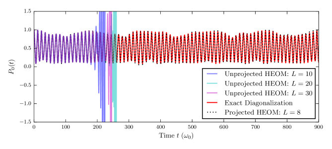
Although there is no guarantee that this projection $\vec{\rho}(t)\rightarrow\bar{\vec{\rho}}(t)$ will not unrecognizably alter the dynamics, it turns out that in cases we have studied for small and intermediate system-bath coupling in discrete-bath models, $\bar{\vec{\rho}}(t)$ rapidly converges to the exact $\vec{\rho}(t)$ as the hierarchy depth is increased. This is unmistakably evident in Fig. 9 , where for the 3-site Holstein model the projection transforms a severely unstable $L=8$ trajectory into what quantitatively resembles the exact dynamics as computed by diagonalization of the Hamiltonian. Similar success is observed for the 2-site Holstein model and the DSB. Since the net effect of unstable modes disappears from the dynamics as $L$ is increased, we interpret these unstable modes as a spurious, unphysical consequence of hierarchy truncation. Meanwhile, since the stable modes with $\Re\left[\lambda_{i}\right]\leq 0$ approach the exact dynamics as $L$ is increased, we interpret these stable modes as corresponding to the physical dynamics, which justifies our projection scheme as a method for obtaining stable, exact dynamics from discrete-bath HEOM.

VI Projecting away instabilities iteratively with Prony filtration

The matrix $A$ in Eq. (35) contains $\tilde{N}^{2}=\left(N^{2}\sum_{n=0}^{L}\frac{(n+2N_{b})!}{n!\left(2N_{b}\right)!}\right)^{2}$ elements(Shi et al., 2009) for the discrete-bath case. Therefore, the $O(\tilde{N}^{3})$ diagonalization-based projection algorithm proposed in V is completely intractable for all but the smallest systems, and only then with sufficiently weak system-bath coupling due to the increased hierarchy depth required to treat stronger system-bath coupling. As such there is a need for approximate or iterative computational techniques for removing unstable modes without requiring an explicit computation of all eigenmodes. Here we discuss one such algorithm. Since (35) is a first order linear differential equation, each hierarchy element may be written as a sum,

$$\rho_{i}(t) =\sum_{j=1}^{\tilde{N}}c_{ij}e^{\lambda_{j}t}\equiv\sum_{j=1}^{\tilde{N}}f_{ij}(t)\equiv\left[\sum_{j=1}^{\tilde{N}}\vec{f}_{j}(t)\right]_{i},$$ (41)

where $c_{ij}$ and $\lambda_{j}$ are complex numbers. The projection in V is equivalent to subtracting off all terms in the sum for which $\Re\left[\lambda_{j}\right]>0$. Consider the following algorithm for subtracting these terms approximately:

1. Numerically integrate the HEOM using an explicit time-stepping algorithm such as fourth-order Runge-Kutta until a time $t_{2}$ when $\max_{i}|\rho_{i}(t_{2})|\gg 1$. It is necessary that by $t_{2}$ one or a small number of modes $\{\vec{F}_{j}\}\subset\{\vec{f}_{j}\}$ have grown many orders of magnitude larger than the other modes.

2. For each hierarchy element, approximate the weights $c_{ij}=\left(\vec{c}_{j}\right)_{i}$ and complex frequencies $\lambda_{j}$ of the dominant modes $\{\vec{F}_{j}\}$ using Beylkin and Monzón’s approximate Prony method(Beylkin and Monzon, 2005). This algorithm for fitting a function to a sum of complex exponential functions is described in detail in section 4 of Beylkin and Monzón(Beylkin and Monzon, 2005).

3. Choose a time $t_{1}<t_{2}$ such that $\max_{i,j}|c_{ij}e^{\lambda_{j}t_{1}}|\ll 1$. Subtract the unstable modes from the hierarchy at time $t_{1}$:

   $$\vec{\rho}(t_{1}) \rightarrow\vec{\rho}(t_{1})-\sum_{j}\vec{c}_{j}e^{\lambda_{j}t_{1}}.$$ (42)

4. Resume numerical integration from time $t_{1}$ until the next instability occurs.

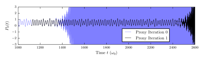
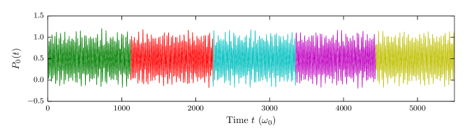
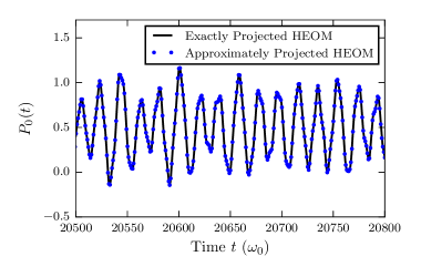
In spirit, this algorithm is similar to excited state methods in quantum mechanics that project out low energy states by imaginary time propagation(Blume et al., 1997). In Fig. 10 we depict a single iteration of the algorithm above. Iterating this “Prony-filtering” algorithm, one can piece together the same projected HEOM solution that would have been provided via a single diagonalization using the approach in V. Such a trajectory is illustrated in Fig. 11 for the DSB; in Fig. 12 we show the corresponding spectrum of $A$, and in Fig. 13 we show the essentially perfect agreement between the diagonalization and Prony-filtering approaches for calculating stable projected dynamics.

Figure 10: Single Prony-filtering iteration for the DSB computed with $L=5$. This plot depicts the electron density on site $0$. First, the blue curve is computed with HEOM. Next, the instability is approximately projected out of the blue trajectory, and then the HEOM simulation is restarted from $t=1120$ at the beginning of the black trajectory to delay the instability until $t>2400$. Model parameters: $g=0.3,\omega_{0}=1,J=0.2,T=0$. Calculations are performed using a modified version of PHI(Strümpfer and Schulten, 2012).

Figure 11: Extension of the Prony-filtered HEOM simulation from Fig. 10. Each color represents a different Prony-filtering iteration, with the instability at times later than $t_{1}$ (see step 3) not depicted. Model parameters: $g=0.3,\omega_{0}=1,J=0.2,T=0$. Calculations are performed using a modified version of PHI(Strümpfer and Schulten, 2012).

Figure 12: Spectrum of $A$ for the DSB at $T=0$ with $L=5$. Model parameters: $g=0.3,\omega_{0}=1,J=0.2$.

Figure 13: Projected HEOM trajectories for the DSB at $T=0$ with $L=5$. Black solid curve uses the diagonalization-based projection. Blue dotted curve uses the approximate Prony-filtered projection; the data shown here is from the 19th Prony iteration of the simulation shown in Fig. 11. Model parameters: $g=0.3,\omega_{0}=1,J=0.2$. Calculations are performed using modified versions of PHI(Strümpfer and Schulten, 2012) and pyrho(Berkelbach, ).

The Prony filtering approach certainly has a significant prefactor due to the cost of Runge-Kutta time-stepping and the approximate Prony analysis of step 2. However, in a similar spirit to the power iteration method or Krylov methods for calculating dominant eigenvectors, this filtration approach has the advantage of not requiring an $O(\tilde{N}^{3})$ diagonalization to compute all of the eigenvectors of $A$. Therefore, the filtering algorithm holds the promise of better scalability compared to the diagonalization-based projection algorithm.

VII Nonnormality of HEOM

Many of the matrices typically encountered in quantum mechanics are Hermitian. Hermitian matrices are diagonalizable and have the properties that all eigenvalues are real, and that the eigenvectors form an orthonormal set, i.e. the matrix is normal. We have already seen that the realness of the eigenvalues is violated for the generator of hierarchy evolution $A$. It turns out that the latter property is also violated.

The nonorthogonality of the eigenmodes in HEOM suggests that removal of instabilities may be ill-conditioned, especially when using deeper hierarchies as is necessary to treat strong coupling. In Fig. 14

Figure 14: Error in computing the eigen-decomposition of $A$ (red, scale on right axis) and condition number of $V$(blue, scale on left axis) as a function of hierarchy depth for the 2-site Holstein model at $T=0$. Model parameters: $g=0.4,\omega_{0}=1,J=0.2$.

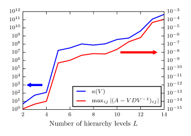
we show how the numerical error in computing the eigen-decomposition $A-VDV^{-1}$ grows as a function of hierarchy depth. This numerical error is not surprising given the nonnormality of $A$, and it explicitly indicates that the diagonalization-based projection in V may be not only expensive, but also ill-conditioned. We also show in Fig. 14 how the condition number of $V$ grows with hierarchy depth. The condition number is defined as

$$\kappa(V) \equiv||V||_{2}\times||V||_{2}^{-1},$$

where the norm $||V||_{2}$ is the largest singular value of $V$. This metric exposes how the linear dependence of the eigenmodes of $A$ grows with hierarchy depth, and it illustrates how their removal via either diagonalization-based projection or Prony filtration may be difficult. For calculating the metrics in Fig. 14 we have employed hierarchy scaling(Shi et al., 2009) with the aim of reducing the diagonalization error and condition number. Although the error is smaller than if we were to use unscaled HEOM, clearly this scaling does not eliminate the growth with hierarchy depth demonstrated in Fig. 14.

In addition to the existence of asymptotic instabilities governed by the spectrum of $A$, it is also possible that numerical instabilities occur at shorter times due to large transient behavior which is characteristic of nonnormal dynamics. A classic example of such numerically unstable transient behavior, as well as its pseudospectral analysis, can be found in a control theory study of Boeing 767 aircraft(Burke et al., 2003; Trefethen and Embree, 2005). We will leave for future work an investigation of whether the HEOM instabilities witnessed for larger Holstein models are caused by such numerically unstable transients or whether they are simply due to the asymptotic growth of the unstable eigenmodes. It is likely that hierarchy scaling(Shi et al., 2009) substantially reduces such transients by scaling down the magnitude of elements deep in the hierarchy.

VIII Concluding remarks

While HEOM is a powerful method that often converges quickly to the numerically exact dynamics over a significant time range, we have shown evidence that HEOM trajectories for both continuous-bath and discrete-bath models at sufficiently low temperature will eventually hit an exponential wall of instability that completely corrupts the description of the time evolution. While this instability can typically be converged away in continuous-bath HEOM, we find that in discrete-bath HEOM deepening the hierarchy does little to delay instabilities, such that novel projection schemes are desired. Two methods, direct and iterative, have been presented to project out the instabilities, and for discrete-bath HEOM it has been shown that the remaining projected solution converges to the exact dynamics without requiring many hierarchy levels. We have discussed challenges that may arise associated with the computational cost and increasing nonnormality of larger and more complex HEOM simulations. As of now, we still lack a complete analytical understanding of the properties of HEOM that lead to the instabilities. We also fall short of a generic scalable solution for removing these instabilities. Perhaps with the advent of new HEOM algorithms such as distributed memory HEOM(Kramer et al., 2018) and matrix product state compressed HEOM(Shi et al., 2018), one may be able to accelerate numerical integration of the HEOM sufficiently to facilitate projection approaches such as the Prony filtration approach introduced here. The challenge of obtaining efficient, stable HEOM solutions will surely benefit from future work that explores alternative closures to the HEOM which reduce the instabilities without corrupting the remaining dynamics, the relation between the breaking of positivity in HEOM(Witt et al., 2017) – as evidenced by the negative populations in this work – and the instabilities, the nature of instabilities in other novel HEOM formulations(Tang et al., 2015; Duan et al., 2017; Nakamura and Tanimura, 2018; Erpenbeck et al., 2018), and computational techniques for removing the unstable modes from nonnormal, unstable linear systems.

Supplementary Material

See supplementary material for animations depicting the spectral dependence of HEOM on hierarchy depth, number of sites, and choice of model.

Appendix - Analytical Treatment of CSB

In this appendix we will use a small analytical example to demonstrate how unstable modes arise in HEOM for the CSB. Consider the HEOM time evolution operator for the CSB with $K=0,L=2$,

$$A =\left[\begin{array}[]{cc}-i\mathcal{L}&\Phi\\ \Theta_{0}&-i\mathcal{L}-\gamma\end{array}\right]=\left[\begin{array}[]{cccccccc}0&-iJ&iJ&0&0&0&0&0\\ -iJ&0&0&iJ&0&2&0&0\\ iJ&0&0&-iJ&0&0&-2&0\\ 0&iJ&-iJ&0&0&0&0&0\\ 2i\lambda\gamma&0&0&0&-\gamma&-iJ&iJ&0\\ 0&-2\lambda\gamma\cot\left(\frac{\beta\gamma}{2}\right)&0&0&-iJ&-\gamma&0&iJ\\ 0&0&2\lambda\gamma\cot\left(\frac{\beta\gamma}{2}\right)&0&iJ&0&-\gamma&-iJ\\ 0&0&0&-2i\lambda\gamma&0&iJ&-iJ&-\gamma\end{array}\right].$$ (53)

If we consider the case $J=0$, we can get closed form expressions for the eigenvalues of $A$:

$$\left\{\lambda_{i}\right\}= \biggr{\{}0,-\gamma,-\frac{1}{2}\left(\gamma+\sqrt{\gamma^{2}-16\lambda\gamma\cot\left(\frac{\beta\gamma}{2}\right)}\right)$$

$$,-\frac{1}{2}\left(\gamma-\sqrt{\gamma^{2}-16\lambda\gamma\cot\left(\frac{\beta\gamma}{2}\right)}\right)\biggr{\}}.$$ (54)

Consider further the case where $\lambda>0,\gamma>0$. The last of these eigenvalues gives rise to an unstable mode whenever

$$\Re\left[-\frac{1}{2}\left(\gamma-\sqrt{\gamma^{2}-16\lambda\gamma\cot\left(\frac{\beta\gamma}{2}\right)}\right)\right] >0.$$ (55)

This condition is equivalent to

$$\cot\left(\frac{\beta\gamma}{2}\right) <0.$$ (56)

This analytical example reveals alternating temperature regions of stability and instability for the CSB, akin to those demonstrated in Figs. 7 and 8, with boundaries located at

$$\beta =\frac{n\pi}{\gamma}$$

$$n =1,2,...$$ (57)

The asymptotes in the cotangent function at $\beta=2n\pi/\gamma$ correspond to an infinite eigenvalue; at such temperatures the HEOM specified by Eq. (53) are completely undefined. Furthermore, for $\beta$ just slightly less than $2n\pi/\gamma$, these HEOM will be exceptionally unstable due to the large magnitude of the last eigenvalue in Eq. (54) near the asymptotes of the cotangent function. On the contrary, for $n\pi<\beta\gamma<\left(n+\frac{1}{2}\right)\pi$ we see that these HEOM are asymptotically stable. These findings agree with the spectral data shown in Figs. 7 and 8.

We should also note that these asymptotes are not present in Fig. 6, since the HEOM in Eq. (17) contain $\coth\left(\beta\omega_{0}/2\right)$ rather than $\cot\left(\beta\gamma/2\right)$ and the hyperbolic cotangent does not contain asymptotes at finite temperatures. Thus, unlike the behavior exhibited in Figs. 7 and 8, that of Fig. 6 is piecewise continuous.

References

- Berne et al. (1998) B. J. Berne, G. Ciccotti, and D. F. Coker, eds., Classical and Quantum Dynamics in Condensed Phase Simulations (World Scientific, Singapore, 1998).
- May and Kühn (2011) V. May and O. Kühn, in Charg. Energy Transf. Dyn. Mol. Syst. (Wiley-VCH Verlag GmbH & Co. KGaA, Weinheim, Germany, 2011).
- Weiss (2012) U. Weiss, Quantum Dissipative Systems, 4th ed. (World Scientific, Singapore, 2012).
- Nitzan (2006) A. Nitzan, Chemical Dynamics in Condensed Phases: Relaxation, Transfer, and Reactions in Condensed Molecular Systems (Oxford University Press, New York, 2006).
- Billing (1975) G. D. Billing, Chem. Phys. Lett. 30, 391 (1975).
- Chen and Reichman (2016) H. T. Chen and D. R. Reichman, J. Chem. Phys. (2016).
- Redfield (1965) A. G. Redfield, Adv. Magn. Opt. Reson. 1, 1 (1965).
- Tanimura and Kubo (1989) Y. Tanimura and R. Kubo, J. Phys. Soc. Japan 58, 101 (1989).
- Ishizaki and Tanimura (2005) A. Ishizaki and Y. Tanimura, J. Phys. Soc. Japan 74, 3131 (2005).
- Ishizaki and Fleming (2009) A. Ishizaki and G. R. Fleming, J. Chem. Phys. 130, 234111 (2009).
- Chen et al. (2009) L. Chen, R. Zheng, Q. Shi, and Y. Yan, J. Chem. Phys. 131 (2009).
- Tanimura (2014) Y. Tanimura, J. Chem. Phys. 141 (2014).
- Feynman and Vernon (1963) R. P. Feynman and F. L. Vernon, Ann. Phys. (N. Y). 24, 118 (1963).
- Makri and Makarov (1995a) N. Makri and D. E. Makarov, J. Chem. Phys. (1995a).
- Makri and Makarov (1995b) N. Makri and D. E. Makarov, J. Chem. Phys. 102, 4611 (1995b).
- Liu et al. (2014) H. Liu, L. Zhu, S. Bai, and Q. Shi, J. Chem. Phys. 140 (2014).
- Chen et al. (2015) L. Chen, Y. Zhao, and Y. Tanimura, J. Phys. Chem. Lett. 6, 3110 (2015).
- Spano (2010) F. C. Spano, Acc. Chem. Res. 43, 429 (2010).
- Bakulin et al. (2016) A. A. Bakulin, S. E. Morgan, T. B. Kehoe, M. W. B. Wilson, A. W. Chin, D. Zigmantas, D. Egorova, and A. Rao, Nat. Chem. 8, 16 (2016).
- Tempelaar and Reichman (2018) R. Tempelaar and D. R. Reichman, J. Chem. Phys. 148, 244701 (2018).
- Fujihashi et al. (2017) Y. Fujihashi, L. Chen, A. Ishizaki, J. Wang, and Y. Zhao, J. Chem. Phys. 146, 044101 (2017).
- Morrison and Herbert (2017) A. F. Morrison and J. M. Herbert, J. Phys. Chem. Lett. 8, 1442 (2017).
- Womick and Moran (2011) J. M. Womick and A. M. Moran, J. Phys. Chem. B 115, 1347 (2011).
- Christensson et al. (2012) N. Christensson, H. F. Kauffmann, T. Pullerits, and T. Mančal, J. Phys. Chem. B 116, 7449 (2012).
- Tiwari et al. (2013) V. Tiwari, W. K. Peters, and D. M. Jonas, Proc. Natl. Acad. Sci. 110, 1203 (2013).
- Tempelaar et al. (2014) R. Tempelaar, T. L. C. Jansen, and J. Knoester, J. Phys. Chem. B 118, 12865 (2014).
- Fröhlich (1954) H. Fröhlich, Adv. Phys. 3, 325 (1954).
- Feynman (1955) R. P. Feynman, Phys. Rev. (1955).
- Feynman et al. (1962) R. P. Feynman, R. W. Hellwarth, C. K. Iddings, and P. M. Platzman, Phys. Rev. (1962).
- Devreese and Alexandrov (2009) J. T. Devreese and A. S. Alexandrov, Reports Prog. Phys. (2009).
- Strümpfer and Schulten (2012) J. Strümpfer and K. Schulten, J. Chem. Theory Comput. 8, 2808 (2012).
- (32) T. Berkelbach, “pyrho: a python package for reduced density matrix techniques,” .
- Kreisbeck et al. (2011) C. Kreisbeck, T. Kramer, M. Rodriguez, and B. Hein, J. Chem. Theory Comput. 7, 2166 (2011).
- Moix and Cao (2013) J. M. Moix and J. Cao, J. Chem. Phys. (2013).
- Holstein (1959a) T. Holstein, Ann. Phys. (N. Y). 8, 343 (1959a).
- Holstein (1959b) T. Holstein, Ann. Phys. (N. Y). 8, 325 (1959b).
- Su et al. (1979) W. P. Su, J. R. Schrieffer, and A. J. Heeger, Phys. Rev. Lett. (1979).
- Mahan (2000) G. D. Mahan, Many-Particle Physics, 3rd ed. (Springer US, Boston, MA, 2000).
- Pekar (1946) S. Pekar, Zhurnal Eksp. I Teor. Fiz. 16, 335 (1946).
- Merrifield (1964) R. E. Merrifield, J. Chem. Phys. 40, 445 (1964).
- Hestand and Spano (2018) N. J. Hestand and F. C. Spano, Chem. Rev. 118, 7069 (2018).
- De Filippis et al. (2015) G. De Filippis, V. Cataudella, A. S. Mishchenko, N. Nagaosa, A. Fierro, and A. De Candia, Phys. Rev. Lett. 114 (2015).
- Munn and Silbey (1985) R. W. Munn and R. Silbey, J. Chem. Phys. 83, 1843 (1985).
- Tanimura and Wolynes (1991) Y. Tanimura and P. G. Wolynes, Phys. Rev. A (1991), 10.1103/PhysRevA.43.4131.
- Xu et al. (2005) R.-X. Xu, P. Cui, X.-Q. Li, Y. Mo, and Y. Yan, J. Chem. Phys. 122, 041103 (2005).
- Shi et al. (2009) Q. Shi, L. Chen, G. Nan, R. X. Xu, and Y. Yan, J. Chem. Phys. 130 (2009), 10.1063/1.
- Jung et al. (1999) Y. Jung, R. J. Silbey, and J. Cao, J. Phys. Chem. A (1999).
- Beylkin and Monzon (2005) G. Beylkin and L. Monzon, Appl. Comput. Harmon. Anal. 19, 17 (2005).
- Blume et al. (1997) D. Blume, M. Lewerenz, P. Niyaz, and K. B. Whaley, Phys. Rev. E (1997).
- Burke et al. (2003) J. V. Burke, A. S. Lewis, and M. L. Overton, IFAC Proc. Vol. 36, 175 (2003).
- Trefethen and Embree (2005) L. N. Trefethen and M. Embree, Spectra and Pseudospectra: The Behavior of Nonnormal Matrices and Operators (Princeton University Press, Princeton, NJ, 2005) pp. 155–157.
- Kramer et al. (2018) T. Kramer, M. Noack, A. Reinefeld, M. Rodríguez, and Y. Zelinskyy, J. Comput. Chem. (2018).
- Shi et al. (2018) Q. Shi, Y. Xu, Y. Yan, and M. Xu, J. Chem. Phys. (2018).
- Witt et al. (2017) B. Witt, L. Rudnicki, Y. Tanimura, and F. Mintert, New J. Phys. (2017), 10.1088/1367-2630/19/1/013007.
- Tang et al. (2015) Z. Tang, X. Ouyang, Z. Gong, H. Wang, and J. Wu, J. Chem. Phys. 143, 224112 (2015).
- Duan et al. (2017) C. Duan, Z. Tang, J. Cao, and J. Wu, Phys. Rev. B 95, 214308 (2017).
- Nakamura and Tanimura (2018) K. Nakamura and Y. Tanimura, Phys. Rev. A 98, 012109 (2018).
- Erpenbeck et al. (2018) A. Erpenbeck, C. Hertlein, C. Schinabeck, and M. Thoss, J. Chem. Phys. 149, 064106 (2018).