Coordinate Descent Full Configuration Interaction

Abstract

We develop an efficient algorithm, coordinate descent FCI (CDFCI), for the electronic structure ground state calculation in the configuration interaction framework. CDFCI solves an unconstrained non-convex optimization problem, which is a reformulation of the full configuration interaction eigenvalue problem, via an adaptive coordinate descent method with a deterministic compression strategy. CDFCI captures and updates appreciative determinants with different frequencies proportional to their importance. We show that CDFCI produces accurate variational energy for both static and dynamic correlation by benchmarking the binding curve of nitrogen dimer in the cc-pVDZ basis with $10^{-3}$ mHa accuracy. We also demonstrate the efficiency and accuracy of CDFCI for strongly correlated chromium dimer in the Ahlrichs VDZ basis and produces state-of-the-art variational energy.

Duke]Department of Mathematics, Duke University Department of Chemistry and Department of Physics, Duke University FCI, CDM, CDFCI

1 Introduction

Solving quantum many-body problem for electrons is a well-known challenging task. While weakly correlated (single-reference) systems can be well approximated using density functional theory and coupled cluster methods such as CCSD(T); strongly corrected (multi-reference) systems remain challenging. The difficulty comes in two aspects: the infamous fermion sign problem and combinatorial scaling of the problem size. In this paper, we propose an efficient algorithm, named coordinate descent FCI (CDFCI), to calculate the ground state energy and its corresponding variational wavefunction for both weakly and strongly correlated fermion systems in the framework of full configuration interaction.

Besides the direct diagonalization of the full configuration interaction (FCI) Hamiltonian ¹, many other algorithms have been proposed, which can be roughly organized into three groups. The first group, density matrix renormalization group (DMRG) ^{2, 3, 4}, adopts tensor train ansatz in representing the variational wavefunction. DMRG has been routinely applied to study the ground and excited state of strongly correlated $\pi$-conjugated molecules and one-dimensional systems ⁴. The second group, like full configuration interaction quantum Monte Carlo (FCIQMC) ^{5, 6, 7}, assumes that the ground state variational wavefunction can be represented as the empirical distribution of a large number of stochastic walkers. To reduce the variance of the energy estimator and the required number of walkers, initiator-FCIQMC (iFCIQMC) ⁸ and semi-stochastic FCIQMC (S-FCIQMC) ⁹ are developed aiming at a good trade-off between variance and bias. The third group first solves a selected configuration interaction (SCI) problem and then conducts a perturbation calculation. This family of algorithms (SCI+PT), includes the early work on configuration interaction by perturbatively selecting iteration (CIPSI) ¹⁰, and more recently, adaptive configuration interaction (ACI) ¹¹, adaptive sampling configuration interaction (ASCI) ¹², etc. Heat-bath configuration interaction (HCI) ¹³ significantly reduces the computational cost of the selected CI phase based on the information from magnitudes of the double excitations. With perturbation, HCI is able to calculate the ground state energy of a strongly correlated all electron chromium dimer up to $1$ mHa accuracy in Ahlrichs VDZ basis. More recently, semi-stochastic HCI (SHCI) ¹⁴ further accelerates the perturbation phase with a stochastic idea similar to FCIQMC.

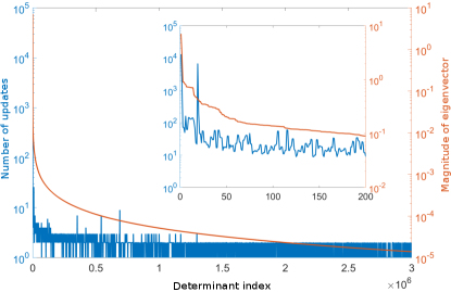
Figure 1: Correlation between the updating frequencies and magnitudes of the ground state wavefunction of an all-electron C2 with cc-pVDZ basis calculated by CDFCI. Coefficients of configuration interaction wavefunction are sorted in a decreasing order based on their magnitudes. Smaller panel shows the results of the largest 200 coefficients.

The algorithm we considered in this paper belongs to the third group (SCI+PT) above. Our goal is to improve the variational stage of the computation i.e., the selective CI part. Our proposed algorithm, CDFCI, is an adaptive coordinate-wise (i.e., determinant-wise) iterative method. It updates the coefficient of an appreciative determinant each iteration and has the nice feature of visiting determinants with different frequencies proportional to their importance. As not all determinants contribute equally to the ground state wavefunction, CDFCI is able to efficiently capture the important part of the FCI space and obtain a good approximation to the ground state. Figure 1 indicates the relation between the updating frequency of determinants and magnitudes of the determinant coefficients of the ground state wavefunction for an all-electron C2 calculation with cc-pVDZ basis by CDFCI. As shown in Figure 1, many coefficients are only updated once throughout iterations, which shows the efficiency of the updating strategy in CDFCI. During iterations, CDFCI also compresses those unappreciative determinants through hard thresholding. Our implementation philosophy of CDFCI is to reserve memory resource for storing variational wavefunction as much as possible, hence, the Hamiltonian matrix is evaluated on-the-fly. Eventually, CDFCI is able to capture the binding curve of all-electron N2 with cc-pVDZ basis up to 6 digits accuracy in one week and compute the ground state energy of all-electron Cr2 with Ahlrichs VDZ basis to $-2086.443565$ Ha, which is the state-of-the-art variational result.

The rest of the paper is organized as follows. Section 2 presents the CDFCI algorithm. The implementation detail is stated in Section 3. In Section 4, we demonstrate the efficiency and accuracy of CDFCI via applying it to various molecules including H2O, C2, N2, and Cr2. Also the binding curve of N2 is characterized. Finally, in Section 5, we conclude the paper together with discussion on future work.

2 Coordinate descent FCI

This section first reformulates the FCI eigenvalue problem as a non-convex optimization problem ^{15, 16} with no spurious local minima and then describes in detail the coordinate descent FCI algorithm together with the compression technique and suggested stopping criteria.

Given a complete set of spin-orbitals $\{\chi_{p}\}$, a many-body Hamiltonian operator, under the second quantization, can be written as

$$\widehat{H}=\sum_{p,q}t_{pq}\hat{a}_{p}^{\dagger}\hat{a}_{q}+\frac{1}{2}\sum_{p,r,q,s}v_{prqs}\hat{a}_{p}^{\dagger}\hat{a}_{r}^{\dagger}\hat{a}_{q}\hat{a}_{s},$$ (1)

where $\hat{a}_{p}^{\dagger}$ and $\hat{a}_{p}$ denote the creation and annihilation operator of an electron with spin-orbital index $p$, $t_{pq}$ and $v_{prqs}$ are one- and two-electron integrals respectively. The ground state energy of $\widehat{H}$ can be obtained from solving the time-independent Schrödinger equation

$$\widehat{H}\ket{\Phi_{0}}=E_{0}\ket{\Phi_{0}},$$ (2)

where $E_{0}$ denotes the ground state energy (the smallest eigenvalue) and $\ket{\Phi_{0}}$ denotes the corresponding ground state wavefunction. Without loss of generality, we assume that $E_{0}$ is negative and non-degenerate, i.e., the eigenvalues of $\widehat{H}$ are given as $E_{0}<E_{1}\leq E_{2}\leq\cdots$.

In FCI, the complete spin-orbital set is truncated to a finite subset $\{\chi_{p}\}_{p=1}^{n_{\text{orb}}}$, obtained e.g., by Hartree-Fock or Kohn-Sham calculations. The FCI variational space $\mathcal{V}$ is spanned by all possible Slater determinants constructed from $\{\chi_{p}\}_{p=1}^{n_{\text{orb}}}$, and the dimension of $\mathcal{V}$ is denoted as $N_{\text{FCI}}$ also known as the total number of configuration interactions. The ground state wavefunction is then discretized in $\mathcal{V}$, i.e., $\ket{\Phi_{0}}\in\mathcal{V}=\,\mathrm{span}\bigl{\{}\ket{D_{1}},\dots,\ket{D_{N_{\text{FCI}}}}\bigr{\}}$, where $\ket{D_{1}}$ denotes the reference determinant, $\ket{D_{i}}$ for $1<i\leq N_{\text{FCI}}$ denotes other Slater determinants constructed from the finite set of spin-orbitals. Correspondingly, the Hamiltonian operator is represented by a many-body Hamiltonian matrix $H$ with its $(i,j)$ entry as $H_{i,j}=\bra{D_{i}}\widehat{H}\ket{D_{j}}$. Let $\boldsymbol{b}$ and $\boldsymbol{c}$ denote coefficient vectors with entry $b_{i}$ and $c_{i}$ respectively. The ground state wavefunction can be written as $\ket{\Phi_{0}}=\sum_{i}c_{i}\ket{D_{i}}$. The time-independent Schrödinger equation (2) has its matrix representation as,

$$H\boldsymbol{c}=E_{0}\boldsymbol{c},$$ (3)

which is known as the FCI eigenvalue problem. The second-quantized Hamiltonian operator as in (1) implies that $H_{i,j}$ is nonzero if and only if $\ket{D_{i}}$ can be obtained from $\ket{D_{j}}$ via changing at most two occupied spin-orbitals. Hence, we say that $\ket{D_{i}}$ is $H$-connected with $\ket{D_{j}}$ if $H_{i,j}$ is nonzero. The set of all indices $i$ such that $\ket{D_{i}}$ is $H$-connected with $\ket{D_{j}}$ is called the $H$-connected index set of $j$ and is denoted as $\mathcal{I}_{H}(j)$. Since the cardinality of $\mathcal{I}_{H}(j)$ is much smaller than $N_{\text{FCI}}$, the matrix $H$ is extremely sparse.

2.1 Reformulation of the FCI eigenvalue problem

The FCI eigenvalue problem (3) can be reformulated as the following unconstrained non-convex optimization problem,

$$\min_{\boldsymbol{c}\in\mathbb{R}^{N_{\text{FCI}}}}f(\boldsymbol{c})=\norm{H+\boldsymbol{c}\boldsymbol{c}^{\top}}_{F}^{2},$$ (4)

where $\norm{\cdot}_{F}$ denotes the Frobenius norm of a matrix. The gradient of the objective function is

$$\nabla f(\boldsymbol{c})=4H\boldsymbol{c}+4\left(\boldsymbol{c}^{\top}\boldsymbol{c}\right)\boldsymbol{c}.$$

As analyzed in our previous work ¹⁶, the stationary points are $\boldsymbol{0}$ and $\pm\sqrt{-E_{i}}\boldsymbol{v}_{i}$ for $E_{i}<0$, where $\boldsymbol{v}_{i}$ is the normalized eigenvector corresponding to $E_{i}$. Furthermore, importantly, $\pm\sqrt{-E_{0}}\boldsymbol{v}_{0}$ are the only two local minimizers with the same objective value, while other stationary points are saddle points. Thus, solving the optimization problem (4) reveals the ground state energy $E_{0}$ and the ground state wavefunction coefficient vector $\boldsymbol{v}_{0}$. For such an optimization problem, higher order methods converge to global minima efficiently but their per iteration computational costs are too expensive for FCI problems. Hence, only first order methods, like gradient descent methods (GDs), stochastic gradient descent methods (SGDs), and coordinate descent methods (CDMs), are discussed here.

The first order optimization methods applied to (4), compared with solving (3) using traditional methods, e.g., power method, Davidson method, and Lanczos method, have two main advantages. First, GDs, SGDs, and CDMs do not need any tuning parameters: no diagonal shift is needed to turn the smallest eigenvalue into the largest one in magnitude ¹⁶ and the stepsize can be addressed by an exact line search. Second, since no orthonormality constraint appears explicitly in (4), solving (4) with GDs, SGDs, and CDMs does not need any orthonormalization step. While in traditional methods like Davidson or Lanczos methods, orthonormalization step is needed every a few iterations to avoid numerical instability issue, which would be expensive for FCI problems.

Among the first order optimization methods, CDMs are more suitable for FCI problems. GDs evaluate and update the exact gradient each iteration, which is prohibitively expensive for FCI problems, due to the huge problem dimension. SGDs evaluate and update a stochastic approximation of the full gradient, which is of much cheaper computational cost per iteration. SGDs actually have been applied to FCI problems in an implicit way: as FCIQMC, iFCIQMC, and S-FCIQMC can all be regarded as SGDs applied to a similar objective function as (4) with constant stepsizes ⁷. SGDs, in general, converge efficiently to a neighborhood of minimizers and then wander around the minimizer due to the stochastic approximation. CDMs select and update a single coefficient each iteration, which is of cheap computational cost. Comparing to GDs, CDMs provably achieve faster convergence rate in terms of the prefactor ¹⁶, whereas comparing to SGDs, CDMs are approximately of equal cost per iteration, but is much more stable towards convergence. Further, with a properly designed selecting strategy, CDMs updates different coefficients with different frequencies, taking advantage of the different importance of determinants in FCI problems. Taking these advantages into consideration, we design CDFCI, which is a CDM tailored for FCI problems with compression strategy, to efficiently solve (4). This method is described in details below.

2.2 Algorithm

The CDFCI algorithm stores two sparse vectors $\boldsymbol{c}^{(\ell)}$ and $\boldsymbol{b}^{(\ell)}$ in the main memory that are contiguously maintained throughout iterations: $\boldsymbol{c}^{(\ell)}$ denotes the computed coefficient vector of the ground state wavefunction in the $\ell$-th iteration and $\boldsymbol{b}^{(\ell)}$ is a compressed approximation of $H\boldsymbol{c}^{(\ell)}$.

Let us first give a sketch of the CDFCI algorithm: In the $\ell$-th iteration, CDFCI first finds the $i^{(\ell+1)}$-th determinant with potentially steepest objective function value decrease among all $H$-connected determinants of $\ket{D_{i^{(\ell)}}}$. Then CDFCI conducts an exact line search to find the optimal update $\alpha$ such that $f(\boldsymbol{c}^{(\ell)}+\alpha\boldsymbol{e}_{i^{(\ell+1)}})$ is minimized and hence the estimator for the ground state energy is reduced, where $\boldsymbol{e}_{i^{(\ell+1)}}$ denotes the indicator vector of $i^{(\ell+1)}$. $\boldsymbol{b}^{(\ell)}$ plays an important role in all above steps. In preparation for next iteration, the vector $\boldsymbol{b}^{(\ell+1)}$ needs to be updated incorporating with $\boldsymbol{c}^{(\ell+1)}=\boldsymbol{c}^{(\ell)}+\alpha\boldsymbol{e}_{i^{(\ell+1)}}$. However, an exact update $\boldsymbol{b}^{(\ell+1)}=\boldsymbol{b}^{(\ell)}+\alpha H_{:,i^{(\ell+1)}}$ could waste limited memory resource on unappreciative determinants. Our compression step updates coefficients only when they do not cost extra memory resource or if they are significantly large in magnitudes. Although the compression step introduces error along the iterations, as we will show, we can still calculate the Rayleigh quotient corresponding to $\boldsymbol{c}^{(\ell+1)}$ exactly, which is used as the ground state energy estimator in CDFCI.

In the following, we will discuss each part of CDFCI in detail and then conclude this section with a pseudo-code for the algorithm.

2.2.1 Determinant-select and coefficient-update

Determinant-select is the first step in each iteration. Assume that the $\ell$-th iteration updates determinant $\ket{D_{i^{(\ell)}}}$ and results in a coefficient vector $\boldsymbol{c}^{(\ell)}$. We select the determinant to be updated at the current iteration, $\ket{D_{i^{(\ell+1)}}}$, according to local information at $\boldsymbol{c}^{(\ell)}$. In order to decrease the objective function value to the largest extent, we could select the determinant with the largest magnitude of the approximated gradient at $\boldsymbol{c}^{(\ell)}$, i.e., $\ket{D_{i^{(\ell+1)}}}$ with

$$i^{(\ell+1)}=\operatorname*{arg\,max}_{j}\absolutevalue{4b^{(\ell)}_{j}+4\left(\left(\boldsymbol{c}^{(\ell)}\right)^{\top}\boldsymbol{c}^{(\ell)}\right)c_{j}^{(\ell)}},$$

where $\boldsymbol{b}^{(\ell)}$ is a compressed approximation of $H\boldsymbol{c}^{(\ell)}$. However, the above strategy requires checking each $j$ (i.e., all determinants), which is prohibitive for even moderate size problems. Hence, instead of checking all determinants, CDFCI only checks the $H$-connected determinants of $\ket{D_{i^{(\ell)}}}$, i.e.,

$$\begin{split}&i^{(\ell+1)}=\\ &\operatorname*{arg\,max}_{j\in\mathcal{I}_{H}(i^{(\ell)})}\absolutevalue{4b_{j}^{(\ell)}+4\left(\left(\boldsymbol{c}^{(\ell)}\right)^{\top}\boldsymbol{c}^{(\ell)}\right)c_{j}^{(\ell)}}.\end{split}$$ (5)

Since our compression strategy introduced later in Section 2.2.2 truncates unappreciative determinants, the expression in (5) remains a good approximation of the exact gradient at $\boldsymbol{c}^{(\ell)}$. Empirically, such a gradient-based determinant-select strategy outperforms other perturbation-based determinant-select strategies as used in other SCI algorithms (see Section 4 for details).

Once the $i^{(\ell+1)}$-th determinant is selected, CDFCI determines the stepsize by the line search along that direction so to decrease the objective function value by the largest amount. Denoting the update as $\alpha$, the line search can be formulated as

$$\alpha=\operatorname*{arg\,min}_{\widetilde{\alpha}\in\mathbb{R}}f(\boldsymbol{c}^{(\ell)}+\widetilde{\alpha}\boldsymbol{e}_{i^{(\ell+1)}}).$$ (6)

Since $h(\widetilde{\alpha})=f(\boldsymbol{c}^{(\ell)}+\widetilde{\alpha}\boldsymbol{e}_{i^{(\ell+1)}})$ is a quartic polynomial in $\widetilde{\alpha}$, solving the minimization problem (6) is equivalent to finding roots of $h^{\prime}(\widetilde{\alpha})$ – the derivative of $h(\widetilde{\alpha})$. If $h^{\prime}(\widetilde{\alpha})$ has a unique root, then the root is the minimizer. If $h^{\prime}(\widetilde{\alpha})$ has two roots, then the one with multiplicity one is the minimizer. If $h^{\prime}(\widetilde{\alpha})$ has three roots, then the one further away from the middle one is the minimizer. Given the update $\alpha$, we can easily update $\boldsymbol{c}^{(\ell)}$ as

$$c_{i}^{(\ell+1)}=\begin{cases}c_{i}^{(\ell)},&i\neq i^{(\ell+1)};\\ c_{i}^{(\ell)}+\alpha,&i=i^{(\ell+1)}.\end{cases}$$ (7)

In CDFCI, we also need to maintain $\boldsymbol{b}^{(\ell+1)}\approx H\boldsymbol{c}^{(\ell+1)}$ for future determinant-select steps. Since only one coefficient is updated in $\boldsymbol{c}^{(\ell)}$, the corresponding $\boldsymbol{b}^{(\ell)}$ can be updated accordingly as,

$$\boldsymbol{b}^{(\ell+1)}\approx H\boldsymbol{c}^{(\ell+1)}\approx\boldsymbol{b}^{(\ell)}+\alpha H_{:,i^{(\ell+1)}}.$$ (8)

Therefore, each update step requires evaluation of all $H$-connections from $\ket{D_{i^{(\ell+1)}}}$. Besides the update from $\boldsymbol{c}^{(\ell+1)}$, we also recalculate the current $i^{(\ell+1)}$-th entry in $\boldsymbol{b}^{(\ell+1)}$ to guarantee the correctness and increase the numerical stability of our algorithm. Such a recalculation could improve the accuracy of the determinant-select (5) and line search (6) in the following iterations, and also provide an accurate Rayleigh quotient as the estimator of the ground state energy as in (11). We argue this correction comes for free in addition to (8), since

$$\begin{split}b_{i^{(\ell+1)}}^{(\ell+1)}=&H_{i^{(\ell+1)},:}\boldsymbol{c}^{(\ell+1)}\\ =&\sum_{j\in\mathcal{I}_{H}(i^{(\ell+1)})}(H_{j,i^{(\ell+1)}})^{\ast}c_{j}^{(\ell+1)},\end{split}$$ (9)

where $(H_{j,i^{(\ell+1)}})^{\ast}$ denotes the complex conjugate of $H_{j,i^{(\ell+1)}}$, which has already been evaluated when updating (8).

2.2.2 Coefficient compression

Since CDFCI initializes $\boldsymbol{c}^{(0)}$ with the reference determinant $\ket{D_{1}}$ and $\boldsymbol{b}^{(0)}=H\boldsymbol{c}^{(0)}$, the coefficient of the reference determinant in $\boldsymbol{b}^{(0)}$ is nonzero and the reference determinant is in $\boldsymbol{b}^{(0)}$. In later iterations, CDFCI is designed to follow one rule: if a determinant is in $\boldsymbol{c}^{(\ell)}$, then it is in $\boldsymbol{b}^{(\ell)}$ as well. Under this rule, if a determinant $\ket{D_{j}}$ is neither in $\boldsymbol{c}^{(\ell)}$ nor in $\boldsymbol{b}^{(\ell)}$, according to (5), this determinant has zero value therein and will not be selected. Hence (5) selects either a new determinant not in $\boldsymbol{c}^{(\ell)}$ but in $\boldsymbol{b}^{(\ell)}$ or an old determinant already in both $\boldsymbol{c}^{(\ell)}$ and $\boldsymbol{b}^{(\ell)}$. In CDFCI, thus, the compression strategy compresses only the unappreciative determinants in $\boldsymbol{b}^{(\ell)}$ to control the computation and memory cost, which in turn restricts the growth of the coefficient vector $\boldsymbol{c}^{(\ell)}$.

Detailed compression strategy is as follows. When a coefficient $\alpha H_{j,i^{(\ell+1)}}$ is added to $b^{(\ell)}_{j}$, we use a predefined tolerance $\varepsilon$ to compress the update. If the $j$-th determinant is already selected before, then $\alpha H_{j,i^{(\ell+1)}}$ is added to $b^{(\ell)}_{j}$ without any compression. If the $j$-th determinant has not been selected in $\boldsymbol{b}^{(\ell)}$, but the update is quantitatively large, i.e., $\absolutevalue{\alpha H_{j,i^{(\ell+1)}}}>\varepsilon$, it indicates that the $j$-th determinant is appreciable and the $j$-th determinant will be added to $\boldsymbol{b}^{(\ell)}$ with the coefficient $\alpha H_{j,i^{(\ell+1)}}$. Otherwise, the update is truncated, i.e., the coefficient in $\boldsymbol{b}^{{(\ell)}}$ remains $0$. The described compression strategy is deterministic and satisfies the rule that determinants with nonzero coefficients in $\boldsymbol{c}^{(\ell)}$ are in $\boldsymbol{b}^{(\ell)}$ as well. For molecules, such a deterministic strategy outperforms other strategies including stochastic compression schemes ¹⁷ due to its effectiveness and cheap cost.

2.2.3 Energy estimation

Although the vector $\boldsymbol{b}^{(\ell+1)}$ is compressed, we emphasize that the Rayleigh quotient $r(\boldsymbol{c})=\frac{\boldsymbol{c}^{\top}H\boldsymbol{c}}{\boldsymbol{c}^{\top}\boldsymbol{c}}$ can be maintained accurately for $\boldsymbol{c}^{(\ell+1)}$, which is used in CDFCI as the estimator of the ground state energy. First, the squared norm of $\boldsymbol{c}^{(\ell)}$ can be updated up to numerical error, i.e.,

$$\left(\boldsymbol{c}^{(\ell+1)}\right)^{\top}\boldsymbol{c}^{(\ell+1)}=\left(\boldsymbol{c}^{(\ell)}\right)^{\top}\boldsymbol{c}^{(\ell)}+2\alpha c_{i^{(\ell+1)}}^{(\ell)}+\alpha^{2}.$$ (10)

An exact update can be computed for the numerator of the Rayleigh quotient as well, i.e.,

$$\begin{split}\left(\boldsymbol{c}^{(\ell+1)}\right)^{\top}H\boldsymbol{c}^{(\ell+1)}=&\left(\boldsymbol{c}^{(\ell)}\right)^{\top}H\boldsymbol{c}^{(\ell)}\\ &+2\alpha b_{i^{(\ell+1)}}^{(\ell+1)}-\alpha^{2}H_{i^{(\ell+1)},i^{(\ell+1)}},\end{split}$$ (11)

where $b_{i^{(\ell+1)}}^{(\ell+1)}$ is recalculated accurately as discussed in Section 2.2.1 around (9). Hence this update is accurate. The Rayleigh quotient of the updated variational wavefunction, $r(\boldsymbol{c}^{(\ell+1)})$ is the ratio of two accurately cumulated quantity and hence accurate. Both in theoretical and numerical results, we observed that the Rayleigh quotient is much more accurate than the projected energy estimator ^{5, 6, 8, 9}, which is $\frac{b_{1}^{(\ell+1)}}{c_{1}^{(\ell+1)}}$ in our notation.

Stopping criteria can be tricky for all iterative methods, including DMRG, FCIQMC, HCI, SHCI, etc, and is also the case for CDFCI. Here we propose three suggestions. As for many iterative methods, we can stop the iteration if the updated value is small. For CDFCI, it is suggested to monitor the cumulated updated values across a few iterations as the stopping criteria. Another stopping criteria is based on the change of the Rayleigh quotient. Usually, we observe monotone decay of the Rayleigh quotient before iteration converges. Therefore, we can stop the algorithm if the decay of the Rayleigh quotient after a few iterations is small. The third suggestion is based on the ratio of the number of nonzero coefficients in $\boldsymbol{b}$ and $\boldsymbol{c}$. When the algorithm converges, this ratio converges to 1. When the ratio is close to $1$, the error introduced by the compression slows down the convergence significantly. Hence more iterations do not make much accuracy improvement. Mixed use of these stopping criteria is suggested in practice.

We conclude this section with a pseudo-code for CDFCI:

1. Initialize $\boldsymbol{c}^{(0)}$ by the reference state $\ket{D_{1}}$ with coefficient being $1$, initialize $\boldsymbol{b}^{(0)}=H\boldsymbol{c}^{(0)}$, and initialize $\ell=0$.

2. Select a determinant with the largest gradient magnitude according to (5). Denote the selected determinant as $\ket{D_{i^{(\ell+1)}}}$.

3. Solve a cubic polynomial equation to obtain the optimal update $\alpha$ for the selected determinant. Update the $i^{(\ell+1)}$-th coefficient as (7).

4. Update $b_{j}^{(\ell+1)}=b_{j}^{(\ell)}+\alpha H_{j,i^{(\ell+1)}}$ if the $j$-th determinant is already selected in $\boldsymbol{b}^{(\ell)}$. Otherwise, add new determinant $\ket{D_{j}}$ to $\boldsymbol{b}^{(\ell+1)}$ with coefficient $\alpha H_{j,i^{(\ell+1)}}$ if $\absolutevalue{\alpha H_{j,i^{(\ell+1)}}}>\varepsilon$. Exactly reevaluate $b_{i^{(\ell+1)}}^{(\ell+1)}$ as (9).

5. Update $\left(\boldsymbol{c}^{(\ell+1)}\right)^{\top}\boldsymbol{c}^{(\ell+1)}$ and $\left(\boldsymbol{c}^{(\ell+1)}\right)^{\top}H\boldsymbol{c}^{(\ell+1)}$ as (10) and (11) respectively. Calculate the exact Rayleigh quotient for $\boldsymbol{c}^{(\ell+1)}$.

6. Repeat 2-5 with $\ell\leftarrow\ell+1$ until some stopping criteria is achieved.

3 Implementation and complexity

We now give some implementation details of the algorithm, focusing on the computationally expensive parts and the numerical stability issues. In the end of this section, a per iteration complexity analysis is conducted.

The indices of Slater determinants are encoded in the way that coincides with that in the second quantization. Suppose there are $n_{\text{orb}}$ spin-orbitals in the FCI discretization, and $n_{\text{e}}$ electrons in the system. Then a Slater determinant is encoded as an $n_{\text{orb}}$-bit binary string, with each bit representing a spin-orbital. The spin-orbital is occupied if the corresponding bit is $1$ and unoccupied if the bit is $0$. The $n_{\text{orb}}$-bit binary string is stored as an array of $64$-bit integers. Thus, $\lceil\frac{n_{\text{orb}}}{64}\rceil$ integers are needed to represent the index of a determinant.

We now focus on the implementation detail of the determinant-update step, as it dominates the runtime. Since the vectors $\boldsymbol{b}$ and $\boldsymbol{c}$ are sparse and compressed in the algorithm, their entries cannot be contiguously stored in memory. For CDFCI, we have tried two different data structure implementations for the combined vector (since the indices of nonzero coefficients of $\boldsymbol{c}$ are contained in $\boldsymbol{b}$, these two vector are stored together in a single data structure): red-black tree and hash table ¹⁸.

Red-black tree is a memory compact representation of the vector: Given that $\boldsymbol{b}$ at current iteration has $n$ nonzero coefficients, red-black tree requires $O(n)$ memory. Inserting, updating and deleting a nonzero coefficient to this red-black tree cost $O(\log n)$ operations. The drawback is that each nonzero coefficient is a node on the tree and hence requires extra memory to store pointers, which turns out to be more expensive comparing to the hash table.

In CDFCI, therefore, we prefer to use a fixed-size open addressing hash table. The hash function mapping a configuration string to an array index is chosen as

$$\mathrm{Hash}(\boldsymbol{d})=\boldsymbol{s}\cdot\boldsymbol{d}\;(\mathrm{mod}\;p),$$ (12)

where the size of the hash table is chosen to be a large prime number $p$; $\boldsymbol{d}$ is the vector of $\lceil\frac{n_{\text{orb}}}{64}\rceil$ integers with bits representing the configuration of the determinant; and $\boldsymbol{s}$ is a fixed vector of the same length as $\boldsymbol{d}$ with entries randomly chosen from $[0,p-1]$ during the CDFCI initialization step. In our current implementation, for each execution of the algorithm, we allocate an array of size approaching machine memory limit for the hash table, which could be modified to enable dynamic resizing feature in order to be memory compact. Inserting, updating and deleting a nonzero coefficient in hash table cost $O(1)$ operations on average; while in the worst case, when the table is almost full, inserting and deleting operation would cost $O(p)$ operations. In order to avoid such inefficient scenarios, we limit the load factor below $80\%$. In practice, these settings of hash table work well and significantly outperform red-black tree. All the numerical results in this paper are produced with hash table.

Besides the expensive data accessing step, the computational expensive step is the evaluation of $H_{:,i^{(\ell+1)}}$. Let $N_{H}=\max_{i}\absolutevalue{\mathcal{I}_{H}(i)}$ be the maximum number of nonzero entries in columns of the Hamiltonian matrix. Although $N_{H}\ll N_{\text{FCI}}$, $N_{H}$ still scales as $O(n_{\text{e}}^{2}n_{\text{orb}}^{2})$. The computational cost for evaluating each entry $H_{i,j}$ also depends moderately on $n_{\text{e}}$. CDFCI uses an efficient Fortran implemented open source quantum chemistry code Hande-QMC as backend for the evaluation of Hamiltonian entries.

Shared memory parallelism based on OpenMP is used in our implementation. For each iteration, the double excitation calculation is the bottleneck for the evaluation $H_{:,i^{(\ell+1)}}$, which is embarrassingly parallelized with OpenMP. In terms of runtime, accessing a nonzero coefficient of $\boldsymbol{b}$ and $\boldsymbol{c}$ is also expensive due to the lack of memory continuity. Therefore, we also parallelize the access to $b_{\mathcal{I}_{H}(i^{(\ell+1)})}$ and $c_{\mathcal{I}_{H}(i^{(\ell+1)})}$ with OpenMP. Due to the possible collision of the hash function of open addressing, we partition the hash array into $2000$ blocks and set locker for each block, such that no two threads can access the same block simultaneously. Increasing the number of lockers would reduce the idling time of threads but would increase the memory cost. We did not try to optimize the number of blocks.

Last point on implementation focuses on the numerical stability of the Rayleigh quotient. Different from other iterative methods, CDFCI updates one determinant per iteration. Hence, for large systems, the number of iteration could easily go beyond $10^{8}$. For cumulated quantities such as $\boldsymbol{c}^{\top}\boldsymbol{c}$ and $\boldsymbol{c}^{\top}H\boldsymbol{c}$, the value is updated at least $10^{8}$ times, hence the accumulated numerical error could pollute the chemical accuracy, and thus careful treatment is needed. In our implementation, we use a quadruple-precision floating point for $\boldsymbol{c}^{\top}\boldsymbol{c}$ and $\boldsymbol{c}^{\top}H\boldsymbol{c}$ such that the relative error is at most $10^{-16}$ unless the number of iteration exceeds $10^{16}$.

Let us remark that our current implementation of CDFCI is by no means optimal. The bottleneck of the current implementation is the naïve hash table. Random access to the main memory is expensive since the cache hierarchy is not fully adapted. An optimized hash table may improve the performance by a big constant.

To conclude the section, let us conduct a leading order per iteration complexity analysis for CDFCI. In determinant-select step, since all $b_{i}^{(\ell)}$ and $c_{i}^{(\ell)}$ for $i\in\mathcal{I}_{H}(i^{(\ell+1)})$ have been accessed in the previous iteration, $i^{(\ell+1)}$ can be computed without paying the cost of accessing the data structure of $\boldsymbol{b}$ and $\boldsymbol{c}$. Hence the leading cost is $O(N_{H})$ with a small prefactor. Line search and updating $\boldsymbol{c}$ cost $O(1)$ operations and are hence negligible. Updating $\boldsymbol{b}$ is the most expensive step throughout the algorithm. It requires evaluating $O(N_{H})$ entries of Hamiltonian matrix and accessing $\boldsymbol{b}$ and $\boldsymbol{c}$ $O(N_{H})$ times. This step costs $O(N_{H})$ operation with a prefactor being the Hamiltonian per entry evaluation cost plus the averaged data structure accessing cost. In our implementation, the compression step is combined with the updating step. Once $H_{:,i^{(\ell+1)}}$ has been evaluated, $b_{i}^{(\ell)}$ and $c_{i}^{(\ell)}$ for $i\in\mathcal{I}_{H}(i^{(\ell+1)})$ are accessed, then exact update of $b_{i^{(\ell+1)}}^{(\ell+1)}$, cumulative updates of $\boldsymbol{c}^{\top}\boldsymbol{c}$ and $\boldsymbol{c}^{\top}H\boldsymbol{c}$ cost $O(N_{H})$ operations with a small prefactor. Overall, CDFCI costs $O(N_{H})$ operations per iteration with the prefactor dominated by the computation cost of one Hamiltonian entry and the averaged access cost of the data structure. The memory cost of CDFCI is dominated by the cost of allocating the data structure.

4 Numerical results

In this section, we perform a sequence of numerical experiments to demonstrate the efficiency of CDFCI. First, we compare the performance of CDFCI, Heat-bath CI (HCI), DMRG and iS-FCIQMC (FCIQMC with initiator and semi-stochastic adaptation) on H2O, C2 and N2 under cc-pVDZ basis. Then, we benchmark the binding curve of nitrogen dimer under cc-pVDZ basis using CDFCI up to $10^{-3}$ mHa accuracy. Finally, we use CDFCI to calculate the ground state energy of chromium dimer Cr2 under the Ahlrichs VDZ Basis at $r=1.5$Å, which is a well-known challenging task due to the strong correlation.

In all experiments, the orbitals and integrals are calculated via restricted Hartree Fock (RHF) in Psi4¹⁹ package. All the reported energies are in Hartree (Ha) but the length unit is in either Bohr radius ($a_{0}$) or ångström (Å) due to different configurations in the references.

4.1 Numerical results of H2O, C2, and N2

We first compare the performance of CDFCI with other algorithms, HCI, DMRG and iS-FCIQMC. In this paper, we choose iS-FCIQMC instead of FCIQMC or iFCIQMC because it balances well among bias, variance and runtime. CDFCI is implemented as stated in Section 3 with the on-the-fly Hamiltonian elements evaluation interfaced from Hande-QMC^{20, 21}. HCI adopts the original implementation in Dice ¹³; DMRG adopts the widely used implementation in Block^{22, 23, 24, 25, 4}; iS-FCIQMC adopts the implementation in NECI code ²⁶. All programs are compiled by Intel compiler 19.0.144 with -O3 option. MPI and OpenMP support are disabled for all programs in this section. All the tests in this section are produced on a machine with Intel Xeon CPU E5-1650 v2 @ 3.50GHz and $64$GB memory. For all algorithms, the Hartree-Fock state is used as the initial wavefunction. Most parameters in CDFCI, HCI, DMRG, and iS-FCIQMC will be clearly stated in the later content. We run HCI with different truncation threshold $\varepsilon_{1}$, DMRG with different maximum bond dimension $\max M$ and iS-FCIQMC with different target population $m$. Any unspecified parameter is set to be the default value. Besides the specified or default parameters, for iS-FCIQMC, the time step is optimized by NECI; the initiator truncation threshold is $3$ and the size of the deterministic space is 1000. For all the tests reported in Table 2, Table 3, and Table 4, iS-FCIQMC runs for $10000$ steps and the energy is estimated by the block analysis in NECI . In all algorithms, the energy is reported without any perturbation or extrapolation post-calculation. Variational energy (Rayleigh quotient) is reported for CDFCI, HCI and DMRG, while average projected energy is reported for iS-FCIQMC. Since iS-FCIQMC is a stochastic method, we also report one significant digit of the Standard Error of the Mean (SEM) in the parenthesis and the SEM is of the same accuracy level as the last digit of the average. SEM is estimated as the sample standard deviation divided by the square root of the sample size. Also Root Mean Square Error (RMSE) of the average estimator is adopted as the error of iS-FCIQMC, which is defined as $\sqrt{\text{standard error}^{2}+\mathrm{bias}^{2}}$. We emphasize that similar perturbation calculation as in HCI can also be applied to CDFCI and the comparison is left as future work.

In this section, we test the four algorithms on three molecules: H2O with OH bond length 1.84345$a_{0}$ and HOH bond angle 110.6° ^{27, 5}, C2 with bond length 1.24253Å ^{13, 28} and N2 with bond length 2.118$a_{0}$ ²⁹. The properties of the systems are summarized in Table 1, where the reference ground state energy is calculated by CDFCI to a high precision.

Molecules	Basis	Electrons	Orbitals	Dimension	HF Energy	GS Energy
H2O	cc-pVDZ	10	24	$4.53\times 10^{8}$	-76.0240386	-76.2418601
C2	cc-pVDZ	12	28	$1.77\times 10^{10}$	-75.4168820	-75.7319604
N2	cc-pVDZ	14	28	$1.75\times 10^{11}$	-108.9493779	-109.2821727

Table 1: Properties of test molecule systems. HF energy and GS energy denote Hartree-Fock energy and ground state energy respectively.

4.1.1 H2O molecule

Table 2 and Figure 2 illustrate numerical results for H2O. In Table 2, we report the detailed results and the corresponding used parameters. Figure 2 plots the convergence of the energy against the wall-clock time based on the results in Table 2. For iS-FCIQMC, we run another test with $m=50000$ for longer time and plot the curve of the projected energy as well as the cumulative average of energy starting at iteration $5000$.

Algorithm	Parameter	Energy	Error	Time(s)	CDFCI
					Time(s)	Ratio
CDFCI	$\varepsilon=0$	-76.2318601	$1.0\times 10^{-2}$	3.7	-
		-76.2408601	$1.0\times 10^{-3}$	96.2	-
		-76.2417601	$1.0\times 10^{-4}$	592.5	-
		-76.2418501	$1.0\times 10^{-5}$	2780.0	-
		-76.2418591	$1.0\times 10^{-6}$	9569.5	-
		-76.2418600	$1.0\times 10^{-7}$	25227.5	-
		-76.2418601	$1.0\times 10^{-8}$	54242.2	-
HCI	$\varepsilon_{1}=1.0\times 10^{-4}$	-76.2412891	$5.7\times 10^{-4}$	58.4	156.3	0.37x
	$\varepsilon_{1}=2.0\times 10^{-5}$	-76.2417533	$1.1\times 10^{-4}$	312.9	565.3	0.55x
	$\varepsilon_{1}=1.0\times 10^{-5}$	-76.2418109	$4.9\times 10^{-5}$	593.5	993.1	0.60x
	$\varepsilon_{1}=5.0\times 10^{-6}$	-76.2418402	$2.0\times 10^{-5}$	1148.3	1823.2	0.63x
DMRG	$\max M=500$	-76.2418170	$4.3\times 10^{-5}$	1731	1089.7	1.59x
	$\max M=1000$	-76.2418557	$4.4\times 10^{-6}$	5224	4435.7	1.18x
	$\max M=2000$	-76.2418596	$4.5\times 10^{-7}$	17839	13802.6	1.29x
	$\max M=4000$	-76.2418599	$1.7\times 10^{-7}$	77023	20585.9	3.74x
iS-FCIQMC	$m=10000$	-76.2418(3)	$2.7\times 10^{-4}$	222.4	277.2	0.80x
	$m=50000$	-76.24197(8)	$1.4\times 10^{-4}$	1009.0	470.5	2.14x
	$m=100000$	-76.24181(5)	$7.1\times 10^{-5}$	1942.8	762.1	2.55x
	$m=500000$	-76.24181(3)	$5.9\times 10^{-5}$	9074.3	875.2	10.37x

Table 2: Convergence of ground state energy of H2O. For CDFCI, we run the test once and report the wall time to reach the accuracy. For other tests, each row corresponds to one test. We also report the wall time for CDFCI to reach the same accuracy as well as the ratio of the wall time of the method over the wall time of CDFCI in the last two columns. iS-FCIQMC runs for $10000$ iterations and reports the average projected energy and the standard error (in parenthesis) through block analysis in the energy column. RMSE is reported as the error of iS-FCIQMC.

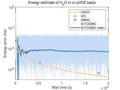
Figure 2: Convergence of ground state energy of H2O against wall clock time. Each point or curve represents one test as in Table 2. For iS-FCIQMC, the projected energy and its cumulative average from iteration $5000$ are plotted with target population $m=50000$.

From Table 2 and Figure 2, we shall see that all algorithms reach chemical accuracy efficiently. CDFCI has a good performance in general. The energy drops quickly to the level of $0.1$ mHa accuracy at the beginning. Then it has a slower but steady linear decay. This behavior proves the rationale behind CDFCI: contributions of different determinants to the FCI energy vary a lot, especially in the early stage of iterations. Since CDFCI always updates the “best” determinant at each iteration, it is able to reach high accuracy with only a few iterations.

For small molecules like H2O, HCI is also an excellent algorithm and costs less time to achieve the same accuracy comparing to CDFCI. It shows that the determinant selecting strategy used in HCI, which relies on decaying property of Hamiltonian entries, is also quite efficient for molecules. For example, when $\varepsilon_{1}=5.0\times 10^{-6}$, HCI uses only $3006594$ determinants to reach $2.0\times 10^{-5}$ Ha accuracy, whereas CDFCI uses $1823176$ determinants, which is about $60\%$ determinants used by HCI to achieve the same accuracy.

The speedup of HCI over CDFCI is due to the different implementation strategies of the algorithms. The implementation of HCI in Dice stores the submatrix of the Hamiltonian with respect to the selected determinants in the main memory, and reuses them for inner Davidson iterations. Both the submatrix and the vector are stored and accessed in contiguous memory. Therefore, two advantages of the implementation come into play: one-time evaluation of Hamiltonian entries and efficient usage of memory hierarchy. However, the disadvantage is also obvious: huge memory cost for the submatrix. In Table 2 and Figure 2, we do not report results for smaller $\varepsilon_{1}$ because Dice reaches the memory limit. The high memory cost is also the reason why the variational stage of HCI does not perform good for chromium dimer (see Section 4.3). As a comparison, CDFCI uses a different philosophy in the implementation. CDFCI calculates the Hamiltonian entries on-the-fly, which saves all memory for the coefficient vector, and stores the coefficients in a hash table. Hence much more coefficients can be used to represent the ground state but paying the cost of repeated evaluation of Hamiltonian entries and limited usage of memory hierarchy.

DMRG also achieves high accuracy in reasonable time with small memory cost. But it is always slower than CDFCI and HCI for H2O.

iS-FCIQMC is very efficient for small number of walkers and iterations. It is able to achieve reasonable accuracy in a short time. In Figure 2 we see the convergence behavior of iS-FCIQMC projected energy. It can reach accuracy level of $1$ mHa very efficiently, but hard to converge to higher accuracy due to the slow convergence of Monte Carlo and the bias introduced by the initiator approximation. It could be possible to use more walkers to reduce the variance and bias. However, as shown in Table 2, moderate increase of the amount of walkers does not change the convergence behavior.

4.1.2 Carbon dimer and nitrogen dimer

Algorithm	Parameter	Energy	Error	Time(s)	CDFCI
					Time(s)	Ratio
CDFCI	$\varepsilon=3.0\times 10^{-8}$	-75.7219604	$1.0\times 10^{-2}$	$49.0$	-
		-75.7309604	$1.0\times 10^{-3}$	$388.2$	-
		-75.7318604	$1.0\times 10^{-4}$	$2687.3$	-
		-75.7319504	$1.0\times 10^{-5}$	$13717.6$	-
		-75.7319594	$1.0\times 10^{-6}$	$55210.2$	-
HCI	$\varepsilon_{1}=1.0\times 10^{-4}$	-75.7305361	$1.4\times 10^{-3}$	100.9	277.8	0.36x
	$\varepsilon_{1}=2.0\times 10^{-5}$	-75.7317130	$2.5\times 10^{-4}$	745.0	1319.1	0.56x
	$\varepsilon_{1}=1.0\times 10^{-5}$	-75.7318541	$1.1\times 10^{-4}$	1261.8	2565.2	0.49x
	$\varepsilon_{1}=5.0\times 10^{-6}$	-75.7319170	$4.4\times 10^{-5}$	2644.3	4989.8	0.53x
DMRG	$\max M=500$	-75.7312704	$6.9\times 10^{-4}$	8624	544.4	15.84x
	$\max M=1000$	-75.7318227	$1.4\times 10^{-4}$	14163	2102.9	6.73x
	$\max M=2000$	-75.7319403	$2.0\times 10^{-5}$	24377	8582.9	2.84x
	$\max M=4000$	-75.7319583	$2.2\times 10^{-6}$	68071	35435	1.92x
iS-FCIQMC	$m=10000$	-75.729(1)	$2.9\times 10^{-3}$	229.5	140.8	1.63x
	$m=50000$	-75.7301(5)	$1.9\times 10^{-3}$	1041.4	212.9	4.89x
	$m=100000$	-75.7314(4)	$7.0\times 10^{-4}$	2038.2	539.8	3.78x
	$m=500000$	-75.7320(1)	$1.5\times 10^{-4}$	9604.2	2003.2	4.79x
	$m=1000000$	-75.7318(1)	$2.1\times 10^{-4}$	18644.8	1497.4	12.45x

Table 3: Convergence of ground state energy of C2. iS-FCIQMC runs for $10000$ iterations and reports the average projected energy and standard error (in parenthesis) through the block analysis in the energy column. RMSE is reported as the error of iS-FCIQMC.

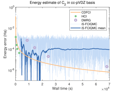
Figure 3: Convergence of ground state energy of C2 against wall clock time. Each point or curve represents one test as in Table 3. For iS-FCIQMC, the projected energy and its cumulative average from iteration $5000$ are plotted with target population $m=500000$.

Algorithm	Parameter	Energy	Error	Time(s)	CDFCI
					Time(s)	Ratio
CDFCI	$\varepsilon=5.0\times 10^{-7}$	-109.2721727	$1.0\times 10^{-2}$	$33.4$	-
		-109.2811727	$1.0\times 10^{-3}$	$752.6$	-
		-109.2820727	$1.0\times 10^{-4}$	$7892.6$	-
		-109.2821627	$1.0\times 10^{-5}$	$49862.6$	-
HCI	$\varepsilon_{1}=1.0\times 10^{-4}$	-109.2805259	$1.7\times 10^{-3}$	100.7	427.1	0.24x
	$\varepsilon_{1}=2.0\times 10^{-5}$	-109.2817822	$3.9\times 10^{-4}$	730.9	2107.4	0.35x
	$\varepsilon_{1}=1.0\times 10^{-5}$	-109.2819787	$1.9\times 10^{-4}$	1335.2	4266.8	0.31x
	$\varepsilon_{1}=5.0\times 10^{-6}$	-109.2820857	$8.7\times 10^{-5}$	3330.0	8920.3	0.37x
DMRG	$\max M=500$	-109.2809830	$1.2\times 10^{-3}$	9936	619.6	16.04x
	$\max M=1000$	-109.2818757	$3.0\times 10^{-4}$	17647	2806.7	6.29x
	$\max M=2000$	-109.2821098	$6.3\times 10^{-5}$	37549	11857.1	3.12x
	$\max M=4000$	-109.2821632	$9.5\times 10^{-6}$	85703	51574.7	1.66x
iS-FCIQMC	$m=10000$	-109.2818(4)	$5.2\times 10^{-4}$	235.7	1556.8	0.15x
	$m=50000$	-109.2822(3)	$2.6\times 10^{-4}$	1068.9	3161.5	0.34x
	$m=100000$	-109.2818(2)	$4.0\times 10^{-4}$	2090.5	2077.2	1.01x
	$m=500000$	-109.2822(1)	$1.2\times 10^{-4}$	9839.3	6832.6	1.44x
	$m=1000000$	-109.28214(5)	$5.0\times 10^{-5}$	18959.7	14510.0	1.31x

Table 4: Convergence of energy of N2. iS-FCIQMC runs for $10000$ iterations and reports the average of projected energy and standard error (in parenthesis) through block analysis. RMSE is reported as the error of iS-FCIQMC.

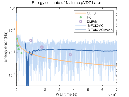
Figure 4: Convergence of ground state energy of N2 against wall clock time. Each point or curve represents one test as in Table 4. For iS-FCIQMC, the projected energy and its cumulative average from iteration $5000$ are plotted with target population $m=500000$.

Carbon dimer C2 and nitrogen dimer N2 are more challenging than H2O molecule since their correlation is stronger and the dimension $N_{\text{FCI}}$ is higher. The results of C2 are reported in Table 3 and Figure 3; and the results of N2 are reported in Table 4 and Figure 4. In general, C2 costs more time than H2O to converge to a fixed accuracy and N2 costs more time than C2, which agrees with their system complexities.

CDFCI shows similar convergence pattern for C2 and N2, with fast decay at the beginning followed by a slower but steady linear decay. It takes only several minutes to reach the chemical accuracy. Therefore, CDFCI is consistently efficient for different systems with different correlation strength.

HCI also shows similar convergence behavior for C2 and N2. It converges to chemical accuracy the fastest among tested algorithms. However, HCI can not converge to higher accuracy due to the memory limit of the implementation. Comparing to CDFCI in terms of the number of operations, however, CDFCI uses less operations and determinants than HCI to the same accuracy level, as in the case of H2O.

DMRG also performs similar for C2 and N2 but is significantly slower than CDFCI and HCI. One reason is that DMRG needs more iterations to converge due to the strong correlation. In this sense, determinant selecting algorithms are less affected by the correlation strength than DMRG.

iS-FCIQMC, however, has a different behavior for C2 and N2. While N2 is significantly harder than C2 for CDFCI, HCI and DMRG, iS-FCIQMC reaches a higher accuracy for N2 within $10000$ iterations, as shown by the data in Table 3 and Table 4. We point out that iS-FCIQMC performs quite well for N2, as it can reach $10^{-4}$ Ha error in a short time with only $m=10000$ or $m=50000$ walkers, whereas CDFCI takes more time to converge since the dimension of N2 is higher than H2O and C2. iS-FCIQMC seems to be less influenced by the increase of dimensionality.

In conclusion, as shown in both Section 4.1.1 and Section 4.1.2, CDFCI is efficient for both weakly-correlated and strongly-correlated systems. It can achieve chemical accuracy efficiently and is able to achieve higher accuracy in all tested molecules. HCI costs more operations than CDFCI to achieve the same accuracy but costs less time due to the different philosophies in implementations. Comparing to CDFCI and HCI, DMRG is less efficient for strongly-correlated systems. While similar as CDFCI, DMRG can also achieve much higher accuracy than the chemical accuracy. iS-FCIQMC is also efficient to reach chemical accuracy with a few walkers in short time for the testing molecules, but it may need much more time and walkers to reach higher accuracy.

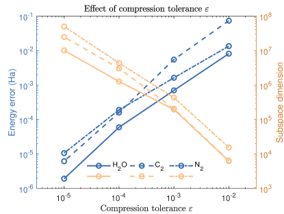
Figure 5: The effect of compression tolerance $\varepsilon$ in CDFCI. The figure shows the error of energy and the number of nonzeros entries in the vector $\boldsymbol{b}$ after convergence for differenct $\varepsilon$. By choosing differenct $\varepsilon$, we can easily balance between accuracy and memory cost.

In terms of the usability, CDFCI, HCI, and DMRG only have one single parameter to be tuned, whereas iS-FCIQMC has more parameters. The proper parameter in CDFCI can be revealed in a few minutes, judging from whether the stabilized vector $\boldsymbol{b}$ properly utilizes the given amount of memory. By choosing $\varepsilon$, we can easily balance between accuracy and memory cost, as shown in Figure 5. We conclude that CDFCI is an easy-to-use efficient algorithm for FCI problems.

4.2 Binding curve of N2

In this section, we benchmark the all-electron nitrogen binding curve using CDFCI under the Dunning’s cc-pVDZ basis. The nitrogen binding curve is a well-known difficult problem. When the nitrogen atoms are stretched away from the equilibrium geometry, Hartree-Fock theory no longer gives a good approximation and the system becomes multi-referenced due to the triple bond between the atoms. DMRG and coupled cluster theory, e.g., CCSD, CCSD(T), CCSDT, etc., have been tested on this problem, but only on 6 geometry configurations ²⁹. Here we show that CDFCI is capable to efficiently benchmark the all-electron nitrogen binding curve on a very fine grid of bond length and the variational energy converges to at least $10^{-3}$ mHa accuracy in each configuration.

In this problem, there are $14$ electrons and $28$ orbitals, and the dimension of the FCI space is about $N_{\text{FCI}}\approx 1.75\times 10^{11}$. In all configurations, $\varepsilon=10^{-6}$ is used in CDFCI for truncation. Here we use the same computing environment as in Section 4.1 but with OpenMP enabled with 5 threads. Each configuration on the bind curve results take roughly one day to achieve the $10^{-3}$ mHa accuracy. Figure 6 shows the binding curve and Table 7 and 8 in Appendix A list all converged variational energies for every configuration in the figure. In Table 5, we compare selected results obtained from CDFCI with that from other algorithms reported in Ref. 29.

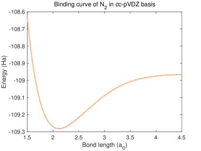
(a) Energy of N2

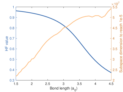
(b) Hartree-Fock value $\boldsymbol{c}_{\mathrm{HF}}/\norm{\boldsymbol{c}}$ and the number of nonzeros of $\boldsymbol{c}$ to reach $10^{-5}$ Ha energy error for CDFCI

Figure 6: Binding curve and the corresponding Hartree-Fock values and number of nonzeros in $\boldsymbol{c}$ of N2 under cc-pVDZ basis.

Bond Length	2.118$a_{0}$	2.4$a_{0}$	2.7$a_{0}$	3.0$a_{0}$	3.6$a_{0}$	4.2$a_{0}$
CDFCI	-109.282173	-109.241908	-109.163600	-109.089405	-108.998083	-108.970132
DMRG	-109.282157	-109.241886	-109.163572	-109.089380	-108.998052	-108.970090
CCSD	-109.267626	-109.219794	-109.131491	-109.052884	-108.975885	-108.960244
CCSDTQ	-109.281943	-109.241321	-109.162264	-109.086502	-108.993736	-108.968124
MRCISD	-109.275356	-109.234925	-109.156473	-109.082149	-108.990759	-108.963070
MRCCSD	-109.280646	-109.240362	-109.161969	-109.087613	-108.995885	-108.967865

Table 5: Nitrogen molecule ground state energy using CDFCI, DMRG ($\max M=4000$) and couple cluster theories. Slant digits indicate inaccurate digits. All results except CDFCI are from Ref. 29.

Several remarks are in order regarding the benchmark results. First, Figure 6 demonstrates a smooth standard shape binding curve. Different from the carbon binding curve ¹³, no jump is observed in our benchmark results, where $D_{2h}$ symmetry is used for all configurations. Second, Table 5 shows that CDFCI gives the lowest energy. CDFCI energy is accurate beyond the level of $10^{-3}$ mHa whereas DMRG is accurate up to $10^{-2}$ mHa. The DMRG results in Table 5 are taken from previous work ²⁹, which agree with the results obtained in Section 4.1.2. Other algorithms such as CCSDTQ are much less accurate. Third, the more the nitrogen dimer molecule is stretched from the equilibrium, the more determinants and iterations are needed for CDFCI to converge to $10^{-3}$ mHa accuracy. This is because Hartree-Fock theory only works well near equilibrium configuration. However, the number of determinants and iterations do not increase significantly, which shows the efficiency of CDFCI again. Other algorithms become less accurate for larger stretching distance.

4.3 All electron chromium dimer calculation

Chromium dimer is hard to compute due to its strong correlation. We calculate the all-electron molecule using CDFCI under the Ahlrichs VDZ basis with radius $r=1.5$Å. There are $48$ electrons and $42$ orbitals, and the dimension of the FCI space is about $2\times 10^{22}$. Many methods have been applied to this problem including DMRG ⁴ and HCI ¹³. Table 6 summarizes all results, including our CDFCI results and others from literature ^{4, 13}.

Algorithm	Energy (Ha)
HCI (variational)	$-2086.{\it 384}$
CCSD(T)	$-2086.4{\it 22229}$
CCSDTQ	$-2086.4{\it 30244}$
DMRG ($\max M=8000$)	$-2086.44{\it 3334}$
CDFCI	$-2086.443{\it 565}$
HCI (perturbed)	$-2086.444{\it 04}$
DMRG (extrapolated)	$-2086.444784$

Table 6: Energy of Cr2.

In this paper, we only consider variational ground state energy without any perturbation or extrapolation. Regarding the variational ground energy, CDFCI achieves lowest energy among all algorithms in one month running time on a machine with Intel Xeon CPU E5-1650 v3 @ 3.50GHz and 128GB memory. Both DMRG ($\max M=8000$) and CDFCI achieve the chemical accuracy if the energy of DMRG (extrapolated) is regarded as the ground truth. But HCI(variational) and coupled cluster theory cannot achieve chemical accuracy. HCI converges to $-2086.384$ Ha in about eight minutes ¹³, whereas CDFCI reaches the same accuracy in about twenty minutes, although different computing environments are used. As the dimension of the Hamiltonian becomes larger and the system becomes more correlated, HCI can only afford storing the submatrix in the main memory with very limited number of determinants and such a limited number cannot achieve higher accuracy in the variational phase. With perturbation phase enabled, HCI can achieve accuracy less than $1$ mHa. Similar perturbation phase can be adapted to CDFCI to further boost the accuracy or extend the applicability of our algorithm to larger systems.

5 Conclusion and discussion

The proposed coordinate descent FCI (CDFCI) is an easy-to-use, accurate, and efficient algorithm for full configuration interaction eigenvalue problems of quantum many-body systems, especially for strongly correlated systems. The only tuning parameter in CDFCI, $\varepsilon$, controls the trade-off between memory cost and accuracy. Given the fixed amount of memory, the “close-to-optimal” $\varepsilon$ can be determined within a few minutes without waiting for convergent results. Hence, we believe that CDFCI is one of the most easy-to-use algorithms among competitors. Besides the user friendly property, CDFCI performs competitively with many other methods, including heat-bath configuration interaction (HCI), density matrix renormalization group (DMRG), and full configuration interaction quantum Monte Carlo with initiator and semi-stochastic adaptation (iS-FCIQMC). The CDFCI can give the state-of-art results for many strongly correlated FCI problems.

There are a few immediate future work of CDFCI. Apply CDFCI to current examples with larger basis sets and other more challenging systems; add perturbation stage to further improve the accuracy; and, parallelize CDFCI in a distributed-memory setting. The earlier two can be accomplished directly, while the massive distributed-memory parallelization of CDFCI requires modification of the greedy determinant-select strategy. Hence FCIQMC type methods currently have some advantage in that regard. As discussed in our previous work ¹⁶, with a stochastic variant of the current determinant-select strategy, the asynchronized feature of coordinate descent methods can be enabled. Massive distributed-memory parallelized CDFCI is expected to achieve good performance. Besides these, we are also exploring (semi-)stochastic CDFCI to improve the parallelizability of the algorithm, and further accelerating the initial iterations. Replacing the current hash function with a more efficient one to fully utilize the memory hierarchy is also under investigation. It is also interesting to design an auto-tuning procedure for “close-to-optimal” $\varepsilon$ to remove the only tuning parameter in the algorithm.

Beyond ground state computation, CDFCI is also suitable for excited state computation. The extension of the optimization problem (4) to low-lying $k$ excited states can be achieved without orthogonality constraint, i.e.,

$$\min_{\boldsymbol{c}\in\mathbb{R}^{N_{\text{FCI}}\times k}}f(\boldsymbol{c})=\norm{H+\boldsymbol{c}\boldsymbol{c}^{\top}}_{F}^{2}.$$ (13)

This is favorable as it removes the expensive orthogonalization step for FCI wavefunctions during iterations. Hence extending CDFCI to solve low-lying excited states is another promising future direction to be explored.

The authors thank Qiming Sun for helpful discussions regarding PySCF and FCI calculations, Ali Alavi for insightful suggestions and for providing all configurations of NECI, and George Booth for helpful discussion on FCIQMC. The work is supported in part by the US National Science Foundation under awards DMS-1454939 and OAC-1450280 and by the US Department of Energy via grant DE-SC0019449.

Appendix A N2 Binding Curve

Figure 6 plots the binding curve of nitrogen dimer in cc-pVDZ basis with data given in Table 7 and Table 8. The bond length of nitrogen dimer in equilibrium geometry is $2.118a_{0}$. Table 7 and Table 8 list variational energies of nitrogen dimer produced by CDFCI with bond lengths smaller and larger than $2.118a_{0}$ respectively. In both tables, CDFCI used $\varepsilon=10^{-6}$ as the truncation threshold.

The bond lengths are selected through the following two steps. CDFCI first calculates energies for a vector of bond lengths linearly spaced between and including $1.50a_{0}$ and $4.50a_{0}$ with gap $0.10a_{0}$. Then, according to the initial rough binding curve, another vector of bond lengths is added to smooth out the curve. These added bond lengths are in the sharp changing range around the equilibrium setting.

Bond length ($a_{0}$)	Energy (Ha)
$1.50$	$-108.6300476$
$1.55$	$-108.7719968$
$1.60$	$-108.8888460$
$1.65$	$-108.9843136$
$1.70$	$-109.0615754$
$1.75$	$-109.1233484$
$1.80$	$-109.1719641$
$1.85$	$-109.2094264$
$1.90$	$-109.2374578$
$1.95$	$-109.2575411$
$2.00$	$-109.2709530$
$2.05$	$-109.2787896$
$2.10$	$-109.2819938$
$2.118$	$-109.2821727$

Table 7: Energy of nitrogen dimer with bond length smaller than that of equilibrium geometry. The energy refers to variational ground state energy calculated by CDFCI with $\varepsilon=10^{-6}$.

Bond length ($a_{0}$)	Energy (Ha)
$2.118$	$-109.2821727$
$2.15$	$-109.2813737$
$2.20$	$-109.2776211$
$2.25$	$-109.2713283$
$2.30$	$-109.2630013$
$2.35$	$-109.2530718$
$2.40$	$-109.2419079$
$2.45$	$-109.2298228$
$2.50$	$-109.2170830$
$2.60$	$-109.1905077$
$2.70$	$-109.1635998$
$2.80$	$-109.1373583$
$2.90$	$-109.1124729$
$3.00$	$-109.0894053$
$3.10$	$-109.0684502$
$3.20$	$-109.0497787$
$3.30$	$-109.0334619$
$3.40$	$-109.0194835$
$3.50$	$-109.0077466$
$3.60$	$-108.9980829$
$3.70$	$-108.9902691$
$3.80$	$-108.9840499$
$3.90$	$-108.9791625$
$4.00$	$-108.9753572$
$4.10$	$-108.9724102$
$4.20$	$-108.9701316$
$4.30$	$-108.9683664$
$4.40$	$-108.9669909$
$4.50$	$-108.9659102$

Table 8: Energy of nitrogen dimer with bond length larger than that of equilibrium geometry. The energy refers to variational ground state energy calculated by CDFCI with $\varepsilon=10^{-6}$.

References

- Knowles and Handy 1984 Knowles, P. J.; Handy, N. C. A new determinant-based full configuration interaction method. Chem. Phys. Lett. 1984, 111, 315–321
- White and Martin 1999 White, S. R.; Martin, R. L. Ab initio quantum chemistry using the density matrix renormalization group. J. Chem. Phys. 1999, 110, 4127
- Chan and Sharma 2011 Chan, G. K.-L.; Sharma, S. The density matrix renormalization group in quantum chemistry. Annu. Rev. Phys. Chem. 2011, 62, 465–481
- Olivares-Amaya \latinet al. 2015 Olivares-Amaya, R.; Hu, W.; Nakatani, N.; Sharma, S.; Yang, J.; Chan, G. K.-L. The ab-initio density matrix renormalization group in practice. J. Chem. Phys. 2015, 142, 034102
- Booth \latinet al. 2009 Booth, G. H.; Thom, A. J. W.; Alavi, A. Fermion Monte Carlo without fixed nodes: A game of life, death, and annihilation in Slater determinant space. J. Chem. Phys. 2009, 131, 054106
- Booth \latinet al. 2012 Booth, G. H.; Grüneis, A.; Kresse, G.; Alavi, A. Towards an exact description of electronic wavefunctions in real solids. Nature 2012, 493, 365–370
- Lu and Wang in press Lu, J.; Wang, Z. The full configuration interaction quantum Monte Carlo method in the lens of inexact power iteration. SIAM J. Sci. Comput. in press, available at http://arxiv.org/abs/1711.09153
- Cleland \latinet al. 2010 Cleland, D.; Booth, G. H.; Alavi, A. Communications: Survival of the fittest: Accelerating convergence in full configuration-interaction quantum Monte Carlo. J. Chem. Phys. 2010, 132, 041103
- Petruzielo \latinet al. 2012 Petruzielo, F. R.; Holmes, A. A.; Changlani, H. J.; Nightingale, M. P.; Umrigar, C. J. Semistochastic projector Monte Carlo method. Phys. Rev. Lett. 2012, 109, 230201
- Huron \latinet al. 1973 Huron, B.; Malrieu, J. P.; Rancurel, P. Iterative perturbation calculations of ground and excited state energies from multiconfigurational zeroth-order wavefunctions. J. Chem. Phys. 1973, 58, 5745–5759
- Schriber and Evangelista 2017 Schriber, J. B.; Evangelista, F. A. Adaptive configuration interaction for computing challenging electronic excited states with tunable accuracy. J. Chem. Theory Comput. 2017, 13, 5354–5366
- Tubman \latinet al. 2016 Tubman, N. M.; Lee, J.; Takeshita, T. Y.; Head-Gordon, M.; Whaley, K. B. A deterministic alternative to the full configuration interaction quantum Monte Carlo method. J. Chem. Phys. 2016, 145, 044112
- Holmes \latinet al. 2016 Holmes, A. A.; Tubman, N. M.; Umrigar, C. J. Heat-bath configuration interaction: An efficient selected configuration interaction algorithm inspired by heat-bath sampling. J. Chem. Theory Comput. 2016, 12, 3674–3680
- Sharma \latinet al. 2017 Sharma, S.; Holmes, A. A.; Jeanmairet, G.; Alavi, A.; Umrigar, C. J. Semistochastic heat-bath configuration interaction method: Selected configuration interaction with semistochastic perturbation theory. J. Chem. Theory Comput. 2017, 13, 1595–1604
- Lei \latinet al. 2016 Lei, Q.; Zhong, K.; Dhillon, I. S. Coordinate-wise power method. Adv. Neural Inf. Process. Syst. 29. 2016; pp 2064–2072
- Li \latinet al. 2018 Li, Y.; Lu, J.; Wang, Z. Coordinate-wise descent methods for leading eigenvalue problem. 2018; \urlhttp://arxiv.org/abs/1806.05647
- Lim and Weare 2017 Lim, L.-H.; Weare, J. Fast randomized iteration: Diffusion Monte Carlo through the lens of numerical linear algebra. SIAM Rev. 2017, 59, 547–587
- Cormen \latinet al. 2009 Cormen, T. H.; Leiserson, C. E.; Rivest, R. L.; Stein, C. Introduction to algorithms, 3rd ed.; The MIT Press, 2009
- Parrish \latinet al. 2017 Parrish, R. M.; Burns, L. A.; Smith, D. G. A.; Simmonett, A. C.; DePrince, A. E.; Hohenstein, E. G.; Bozkaya, U.; Sokolov, A. Y.; Di Remigio, R.; Richard, R. M.; Gonthier, J. F.; James, A. M.; McAlexander, H. R.; Kumar, A.; Saitow, M.; Wang, X.; Pritchard, B. P.; Verma, P.; Schaefer, H. F.; Patkowski, K.; King, R. A.; Valeev, E. F.; Evangelista, F. A.; Turney, J. M.; Crawford, T. D.; Sherrill, C. D. Psi4 1.1: An Open-Source Electronic Structure Program Emphasizing Automation, Advanced Libraries, and Interoperability. J. Chem. Theory Comput. 2017, 13, 3185–3197
- Spencer \latinet al. 2015 Spencer, J. S.; Blunt, N. S.; Vigor, W. A.; Malone, F. D.; Foulkes, M. C.; Shepherd, J. J.; Thom, A. J. W. Open-source development experiences in scientific software: The HANDE quantum Monte Carlo project. J. Open Res. Softw. 2015, 3
- Spencer \latinet al. in press Spencer, J. S.; Blunt, N. S.; Choi, S.; Etrych, J.; Filip, M.-A.; Foulkes, W. M. C.; Franklin, R. S. T.; Handley, W. J.; Malone, F. D.; Neufeld, V. A.; Di Remigio, R.; Rogers, T. W.; Scott, C. J. C.; Shepherd, J. J.; Vigor, W. A.; Weston, J.; Xu, R.; Thom, A. J. The HANDE-QMC project: open-source stochastic quantum chemistry from the ground state up. J. Chem. Theory Comput. in press, available at https://doi.org/10.1021/acs.jctc.8b01217
- Chan and Head-Gordon 2002 Chan, G. K.-L.; Head-Gordon, M. Highly correlated calculations with a polynomial cost algorithm: A study of the density matrix renormalization group. J. Chem. Phys. 2002, 116, 4462–4476
- Chan 2004 Chan, G. K.-L. An algorithm for large scale density matrix renormalization group calculations. J. Chem. Phys. 2004, 120, 3172–3178
- Ghosh \latinet al. 2008 Ghosh, D.; Hachmann, J.; Yanai, T.; Chan, G. K.-L. Orbital optimization in the density matrix renormalization group, with applications to polyenes and -carotene. J. Chem. Phys. 2008, 128, 144117
- Sharma and Chan 2012 Sharma, S.; Chan, G. K.-L. Spin-adapted density matrix renormalization group algorithms for quantum chemistry. J. Chem. Phys. 2012, 136, 124121
- Booth \latinet al. 2014 Booth, G. H.; Smart, S. D.; Alavi, A. Linear-scaling and parallelisable algorithms for stochastic quantum chemistry. Molecular Physics 2014, 112, 1855–1869
- Olsen \latinet al. 1998 Olsen, J.; Jørgensen, P.; Koch, H.; Balkova, A.; Bartlett, R. J. Full configuration-interaction and state of the art correlation calculations on water in a valence double-zeta basis with polarization functions. J. Chem. Phys. 1998, 104, 8007
- Sharma and Alavi 2015 Sharma, S.; Alavi, A. Multireference linearized coupled cluster theory for strongly correlated systems using matrix product states. J. Chem. Phys. 2015, 143, 102815
- Chan \latinet al. 2004 Chan, G. K.-L.; Kállay, M.; Gauss, J. State-of-the-art density matrix renormalization group and coupled cluster theory studies of the nitrogen binding curve. J. Chem. Phys. 2004, 121, 6110–6116
- Wright 2015 Wright, S. J. Coordinate descent algorithms. Math. Program. 2015, 151, 3–34
- Wang \latinet al. 2018 Wang, J.; Wang, W.; Garber, D.; Srebro, N. Efficient coordinate-wise leading eigenvector computation. Proc. Algorithmic Learn. Theory, PMLR. 2018; pp 806–820
- Sun \latinet al. 2018 Sun, Q.; Berkelbach, T. C.; Blunt, N. S.; Booth, G. H.; Guo, S.; Li, Z.; Liu, J.; McClain, J. D.; Sayfutyarova, E. R.; Sharma, S.; Wouters, S.; Chan, G. K.-L. PySCF: the python-based simulations of chemistry framework. Wiley Interdiscip. Rev. Comput. Mol. Sci. 2018, 8, e1340
Appendix A \chN2 Binding Curve