Scattering mechanisms and electrical transport near an Ising nematic quantum critical point

Abstract

Electrical transport properties near an electronic Ising-nematic quantum critical point in two dimensions are of both theoretical and experimental interest. In this work, we derive a kinetic equation valid in a broad regime near the quantum critical point using the memory matrix approach. The formalism is applied to study the effect of the critical fluctuations on the dc resistivity through different scattering mechanisms, including umklapp, impurity scattering, and electron-hole scattering in a compensated metal. We show that electrical transport in the quantum critical regime exhibits a rich behavior that depends sensitively on the scattering mechanism and the band structure. In the case of a single large Fermi surface, the resistivity due to umklapp scattering crosses over from $\rho\sim T^{2}$ at low temperature to sublinear at high temperature. The crossover temperature scales as $q_{0}^{3}$, where $q_{0}$ is the minimal wavevector for umklapp scattering. Impurity scattering leads to $\rho-\rho_{0}\sim T^{\alpha}$ ($\rho_{0}$ being the residual resistivity), where $\alpha$ is either larger than $2$ if there is only a single Fermi sheet present, or $4/3$ in the case of multiple Fermi sheets. Finally, in a perfectly compensated metal with an equal density of electrons and holes, the low temperature behavior depends strongly on the structure of “cold spots” on the Fermi surface, where the coupling between the quasiparticles and order parameter fluctuations vanishes by symmetry. In particular, for a system where cold spots are present on some (but not all) Fermi sheets, $\rho\sim T^{5/3}$. At higher temperatures there is a broad crossover regime where $\rho$ either saturates or $\rho\sim T$, depending on microscopic details. We discuss these results in the context of recent quantum Monte Carlo simulations of a metallic Ising nematic critical point, and experiments in certain iron-based superconductors.

I Introduction

Many strongly correlated materials, such as high temperature superconductors, exhibit electrical transport properties that are markedly different from those expected in a Fermi liquid. Most famously, in many systems, the electrical resistivity is a linear function of temperature. Interestingly, it is often in this regime where the highest superconducting transition temperature is observed. Understanding the role of strong electronic correlations in such systems is of utmost importance. A natural way to explain these properties is to consider a metallic system tuned near a quantum critical point (QCP), i.e., a “quantum critical metal”. This is further motivated by the observation that superconductivity is typically found near another electronically ordered phase Scalapino (2012). The electronic order is suppressed by varying an external parameter such as electron concentration or pressure, leading to a putative QCP. The critical fluctuations of the order parameter mediate long-range, dynamical interactions between electrons. These interactions can lead to a breakdown of Fermi liquid behavior at the longest length and timescales.

Of particular interest is the electrical transport properties near an Ising-nematic QCP in two spatial dimensions Dell’Anna and Metzner (2007); Hartnoll et al. (2014); Lederer et al. (2017); Maslov et al. (2011). An Ising nematic phase refers to a rotation-symmetry-breaking electronic order where the square lattice tetragonal symmetry is spontaneously broken down to orthorhombic. It has been observed in various condensed matter systems Fradkin et al. (2010), notably in various high $T_{c}$ superconductors, including iron pnictides Chu et al. (2010); Fernandes et al. (2014) and iron chalcogenides Hosoi et al. (2016); Coldea and Watson (2018). Evidence for nematic fluctuations has been found in the cuprate superconductors, as well Kohsaka et al. (2007); Daou et al. (2010). Recent experiments Kasahara et al. (2010); Reiss et al. (2017); Urata et al. (2016); Reiss et al. reported non-Fermi liquid transport in the vicinity of the nematic QCP.

On the theoretical front, several works have studied trasport near a nematic QCP Dell’Anna and Metzner (2007); Hartnoll et al. (2014); Maslov et al. (2011); Lederer et al. (2017), along with many other investigations of transport in different types of quantum critical metals Varma et al. (1989); Kim et al. (1995); Hlubina and Rice (1995); Rosch (1999); Syzranov and Schmalian (2012); Paul et al. (2013); Patel and Sachdev (2014); Chubukov et al. (2014); Chubukov and Maslov (2017). However, the general picture remains unclear. Naively, since the singular fluctuations of the nematic order parameter occur at small wavevectors, one may expect them not to strongly modify transport properties. Treating the order parameter fluctuations as an external “bath”, Ref. Dell’Anna and Metzner (2007) found a resistivity that varies as $T^{3/2}$ near the QCP. However, in an electronic nematic transition, the order parameter fluctuations are a collective mode of the same electrons that carry the current. This issue was addressed in Ref. Maslov et al. (2011), and the resistivity was found to vary as $T^{2}$ in the clean case, due to the long-wavelength nature of the nematic fluctuations. Ref. Hartnoll et al. (2014) treated the case where the main source of momentum relaxation is long-wavelength disorder that couples to the order parameter as a random field; a variety of behaviors was found depending on the dynamical critical exponent assumed for the QCP. Indications for non-Fermi liquid transport due to quantum critical nematic fluctuations were found in recent numerical simulations Lederer et al. (2017); however, these result suffer from the usual uncertainties associated with analytical continuation of numerical data, and need to be backed by analytical calculations. Clearly, a uniform theoretical framework to treat transport near an Ising-nematic QCP is highly desireable.

The situation is complicated by the fact that despite the substantial progress made  Metzner et al. (2003); Oganesyan et al. (2001); Rech et al. (2006); Lawler et al. (2006); Löhneysen et al. (2007); Lee (2009); Zacharias et al. (2009); Mross et al. (2010); Metlitski and Sachdev (2010); Dalidovich and Lee (2013); Holder and Metzner (2015); Klein et al. (2018a, b), the theory of Ising-nematic quantum criticality at asymptotically low energies is not well understood. However, as we argue below, there is a broad range of energy scales where the theory can be controlled; this “Hertz–Millis–Moriya” regime is described in terms of coherent electrons interacting with strongly renormalized, overdamped collective fluctuations of the order parameter Hertz (1976); Millis (1993); Moriya (1985). Evidence for the existence of such a regime has been found in recent quantum Monte Carlo simulations Schattner et al. (2016); Lederer et al. (2017); Berg et al. (2019). At lower temperatures, the theory becomes strongly coupled, with nematic-mediated superconducting fluctuations and strong non-Fermi liquid behavior onsetting at the same energy scale.

In this work, we develop a memory matrix approach for transport in the intermediate coherent electron regime. Transport in this regime can be described by a kinetic equation, where the effects of the quantum critical fluctuations are incorporated in the collision integral. At low temperatures (in the absence of a superconducting phase), the electrons become incoherent, and our approach breaks down; however, in the absence of a magnetic field, in this regime the system generically becomes a high $T_{c}$ superconductor mediated by the nematic fluctuations. Our theory is expected to hold down to temperatures of the order of $T_{c}$.

We apply our technique to study situations where different scattering mechanisms dominate the transport behavior, including umklapp scattering, impurity scattering, and momentum-conserving electron-hole scattering in a compensated metal. We find that depending on the relaxation mechanism, the electrical resistivity exhibits rich features, including several regimes beyond the ones discussed in Refs. Dell’Anna and Metzner (2007); Maslov et al. (2011). Our main results are summarized as follows:

1. In a clean system with a large, generic Fermi surface, umklapp scattering has a low-momentum threshold $q_{0}$ determined by the smallest distance between Fermi surfaces in different Brillouin zones. At low temperatures, $T\ll T_{0}\sim q_{0}^{3}$, the typical momentum of the quantum critical fluctuations is smaller than $q_{0}$. As a result, $\rho(T)\sim T^{2}$, as in a Fermi liquid, despite the proximity to the QCP Maslov et al. (2011). At higher temperatures, umklapp scattering is governed by critical fluctuations. In this regime, $\rho(T)$ is strongly enhanced, and the dynamics of the critical fluctuations is qualitatively modified by the umklapp processes, and deviates from the naive low-temperature scaling behavior (characterized by a $z=3$ dynamical critical exponent). As a result, $\rho(T)$ exhibits a smooth crossover from $T^{2}$ at $T\ll T_{0}$ to sublinear at higher temperatures.

2. In the presence of weak impurity scattering in a single electronic band and in the absence of umklapp scattering, the critical nematic fluctuations decouple from the transport properties to lowest order in temperature. This is since for a single convex Fermi surface, electron-electron scattering near the Fermi surface conserves the odd moments of the quasiparticle distribution function Maslov et al. (2011); Ledwith et al. (2017). Therefore, to lowest order, $\rho(T)=\rho_{0}$, and the correction scales as $T^{\beta}$ with $\beta>2$. However, for a generic multiband system, we find $\rho(T)-\rho_{0}\propto T^{4/3}$ due to quantum critical fluctuations.

3. For a clean compensated metal with an equal density of electrons and holes, the low-tempearture properties are strongly sensitive to the presence of “cold spots” on the Fermi sheets. At these points, the lowest-order coupling between the quasiparticles and the nematic fluctuations vanishes by symmetry. For instance, in the case of a $B_{1g}$ nematic order parameter (of $x^{2}-y^{2}$ symmetry), the cold spots occur at the intersection between the diagonals $k_{x}=\pm k_{y}$ and the Fermi surfaces. We show that the non-equilibrium distribution function displays a strongly non-harmonic form, changing abruptly at the cold spots. In the case where all the Fermi surfaces have cold spots, $\rho\sim T^{2}$; if only some of the Fermi surfaces have cold spots and others do not , then $\rho\sim T^{5/3}$. If none of the Fermi surfaces have cold spots, then $\rho\sim T^{4/3}$. At intermediate to strong coupling strengths , there is a broad crossover regime where the resistivity either saturates or is linear in temperatrure, depending on microscopic details. The crossover behavior is due to near elastic scattering of electrons by thermal nematic fluctuations.

The outline of the paper is given as follows. In Section II, we introduce a model Hamiltonian that realizes a metallic Ising-nematic QCP, and argue that there is a parametrically broad temperature regime where electrical transport can be described by kinetic theory. In Section III, we derive a memory matrix formalism for calculating the linearized collision integral, and discuss various conservation laws. In Section IV, we study the temperature dependence of dc electrical resistivity near the QCP originating from various current-relaxation mechanisms, including impurity scattering, umklapp scattering, and momentum conserving electron-hole scattering in a compensated metal. We conclude in Section V.

II Model

We consider a simple model on a two-dimensional square lattice that realizes a metallic Ising-nematic QCP. The Hamiltonian is given by

$$\begin{split}H=&\sum_{\mathbf{k},\alpha=1}^{N}\left(\varepsilon_{\mathbf{k}}-\mu\right)c_{\alpha\mathbf{k}}^{\dagger}c_{\alpha\mathbf{k}}-\frac{1}{2}\sum_{\mathbf{q}}U_{\mathbf{q}}Q_{\mathbf{q}}Q_{-\mathbf{q}}\end{split}$$ (1)

where

$$Q_{\mathbf{q}}=\sum_{\mathbf{k},\alpha}f_{\mathbf{k},\mathbf{k+q}}c_{\alpha\mathbf{k}+\mathbf{q}}^{\dagger}c_{\alpha\mathbf{k}}.$$ (2)

Here, $c_{\alpha\mathbf{k}}$ annihilates an electron of flavor $\alpha=1,\dots,N$ with momentum $\mathbf{k}$. $\varepsilon_{\mathbf{k}}$ is the electron’s energy dispersion, and $\mu$ is the chemical potential. Physically, $N=2$ (for the two spin flavors), but we will keep $N$ general – for some purposes it will be useful to consider the limit of large $N$. The nematic form factor $f_{\mathbf{k},\mathbf{k+q}}$ satisfies $f_{\mathbf{k},\mathbf{k+q}}=-f_{\mathcal{R}_{\pi/2}\mathbf{k},\mathcal{R}_{\pi/2}(\mathbf{k+q})}$, where $\mathcal{R}_{\pi/2}$ is a rotation by $\pi/2$ around the axis perpendicular to the plane. The interaction is written as $U_{\mathbf{q}}=\lambda^{2}D_{0,\mathbf{q}}/N$, where $\lambda$ is the coupling constant (the normalization by $N$ enables us to define the large-$N$ limit), and we choose $D_{0,\mathbf{q}}=1/[r_{0}+2(2-\cos q_{x}-\cos q_{y})]$ (the lattice constant is set to unity) . $r_{0}$ is a tuning parameter used to approach the QCP.

Following the standard procedure, we use a Hubbard-Stratonovich transformation with a real scalar field $\phi$ to decouple the interaction term, obtaining the Lagrangian

$$L=L_{0}+\frac{1}{2}\sum_{\mathbf{q}}D_{0,\mathbf{q}}^{-1}|\phi_{\mathbf{q}}|^{2}+\frac{\lambda}{\sqrt{N}}\sum_{\mathbf{q}}\phi_{-\mathbf{q}}Q_{\mathbf{q}},$$ (3)

where $L_{0}$ is a free fermion Lagrangian corresponding to the first term in Eq. (1). The field $\phi$ can be thought of as describing the spatial and temporal fluctuations of the nematic order parameter; in the nematic phase, $\langle\phi\rangle\neq 0$.

The low-energy continuum field theory governing the critical behavior has been studied extensively Metlitski and Sachdev (2010). Here we briefly summarize the physical picture in the vicinity of the QCP:

1. The nematic fluctuations become overdamped as a result of their coupling to electrons near the Fermi surface. To leading order in $\lambda$, $\phi$ acquires a self-energy of the form: $\Pi(\mathbf{q},i\nu_{n})\propto f_{\mathbf{q},\mathbf{q}}^{2}\frac{\gamma|\nu_{n}|}{|\mathbf{q}|}$, where $\nu_{n}=2\pi Tn$ is the bosonic Matsubara frequency and $\gamma\propto\lambda^{2}\varepsilon_{F}^{-2}$ is the Landau-damping coefficient ($\varepsilon_{F}$ is the Fermi energy). This leads to a quantum critical scaling with a dynamical critical exponent $z=3$.

2. The feedback of the Landau-damped critical fluctuations on the electrons near the Fermi surface leads, to one-loop order, to an electronic self-energy $\Sigma(\mathbf{k},i\omega_{n})\propto f_{\mathbf{k},\mathbf{k}}^{2}\varepsilon_{F}N^{-1}|\gamma\omega_{n}|^{2/3}$, where $\omega_{n}=2\pi T\left(n+\frac{1}{2}\right)$ is the fermionic Matsubara frequency. Below an energy scale $\Omega_{\text{NFL}}\propto\lambda^{4}\varepsilon_{F}^{-1}N^{-3}$, the self-energy becomes dominant over the bare $i\omega_{n}$ term in the electron propagator, and the electrons become strongly incoherent. This regime is currently not well understood theoretically. Within a large–$N$ expansion, terms which are naively of arbitrarily high order in $1/N$ turn out to be equally important as the leading ones in this regime. Superconducting fluctuations are also expected to become strong at the same energy scale, implying a nematic-mediated superconducting transition temperature $T_{c}\sim\Omega_{\text{NFL}}$. A dome-shaped superconducting phase with a maximum $T_{c}$ near the nematic QCP was indeed found in quantum Monte Carlo simulations Lederer et al. (2017); Berg et al. (2019).

These considerations suggest that in the weak coupling limit $\lambda^{2}\ll\varepsilon_{F}$ or in the large–$N$ limit, there is a broad regime of temperatures $\Omega_{\text{NFL}}\ll T\ll\varepsilon_{F}$ above the QCP where the system can be described in terms of Landau-damped nematic fluctuations coupled to coherent electrons. Evidence for the existence of such a regime, even at moderate values of the coupling constant, has been found in numerical simulations Schattner et al. (2016). In this regime, the use of a kinetic equation approach for computing transport properties is justified, with the effects of the scattering off critical fluctuations incorporated in the collision integral.

III Method

In the previous section, we argued that above an energy scale $\Omega_{\text{NFL}}$, the normal state transport is governed by a kinetic (Boltzmann) equation. Deriving the kinetic equation requires special care: while the Lagrangian in Eq. (3) describes electrons coupled to a fluctuating boson $\phi_{\mathbf{q}}$, it is important to keep track of the fact that the bosonic degrees of freedom do not act as a “bath” for the electrons; rather, they are collective modes of the same electron fluid [as is manifest in the original Hamiltonian in Eq. (1)]. Therefore, in the absence of an external momentum relaxation mechanism (such as umklapp or impurity scattering), the total electronic momentum is conserved.

In this section, we derive the kinetic equation based on the memory matrix method. This method has been applied widely for studying transport phenomena; see, e.g., Refs. Kadanoff and Martin (1963); Forster (March 8, 2018); Götze and Wölfle (1972); Rosch and Andrei (2000); Shimshoni et al. (2003); Jung and Rosch (2007); Mahajan et al. (2013); Lucas and Sachdev (2015); Hartnoll et al. (2018). It has the advantage that the “collision term” in the kinetic equation is formulated as a correlation function at equilibrium, that can be computed using standard perturbative techniques.

The dc resistivity can be calculated by taking the zero-frequency limit of the real part of optical conductivity, i.e., $\rho^{-1}=\lim_{\Omega\rightarrow 0}\text{Re}\sigma(\Omega)$. Within linear response, the optical conductivity is given by the retarded current-current correlation function: $\sigma(\Omega)=\frac{1}{i\Omega}\left[G_{J_{x}J_{x}}^{R}\left(\Omega\right)-G_{J_{x}J_{x}}^{R}\left(0\right)\right]$, where $\mathbf{J}$ is the electrical current operator corresponding to Eq. (1), obtained through replacing $c_{\alpha\mathbf{k}}\rightarrow c_{\alpha\mathbf{k}+e\mathbf{A}}$ and taking $\mathbf{J}=\partial H/\partial\mathbf{A}$. To lowest order in $\lambda$ or in $1/N$, $\mathbf{J}\approx\sum_{\mathbf{k,\alpha}}\mathbf{v}_{\mathbf{k}}c_{\alpha\mathbf{k}}^{\dagger}c_{\alpha\mathbf{k}}$ .

Within the memory matrix method, the dynamics is projected onto a set of “slow operators” that are nearly conserved by the Hamiltonian. We briefly review the method in Appendix A.1. In our model, the operators $n_{\alpha\mathbf{k}}=c_{\alpha\mathbf{k}}^{\dagger}c_{\alpha\mathbf{k}}$ are nearly-conserved in the limit of either small $\lambda$ or large $N$ . The optical conductivity can then be cast in the form:

$$\sigma(\Omega)=\sum_{\alpha,\beta,\mathbf{k},\mathbf{k^{\prime}}}\chi_{J_{x},\alpha\mathbf{k}}\left(\frac{1}{M(\Omega)-i\Omega\chi}\right)_{\alpha\mathbf{k},\mathbf{\beta k^{\prime}}}\chi_{\beta\mathbf{k}^{\prime},J_{x}}$$ (4)

where $\chi_{J_{x},\alpha\mathbf{k}}\equiv\int_{0}^{\beta}\mathrm{d}\tau\langle J_{x}(\tau)n_{\alpha\mathbf{k}}(0)\rangle$ and $\chi_{\alpha\mathbf{k},\beta\mathbf{k^{\prime}}}\equiv\int_{0}^{\beta}\mathrm{d}\tau\left[\langle n_{\alpha\mathbf{k}}(\tau)n_{\beta\mathbf{k^{\prime}}}(0)\rangle-\langle n_{\alpha\mathbf{k}}\rangle\langle n_{\beta\mathbf{k^{\prime}}}\rangle\right]$ are thermodynamic susceptibilities. The dynamical properties are encoded in the structure $\left[M(\Omega)-i\Omega\chi\right]^{-1}$, where $M_{\alpha\mathbf{k},\beta\mathbf{k}^{\prime}}(\Omega)$ is the “memory matrix”. To leading order in $1/N$, the memory matrix is given by:

$$M_{\alpha\mathbf{k},\beta\mathbf{k^{\prime}}}(\Omega)=\frac{1}{i\Omega}\left[G_{\dot{n}_{\alpha\mathbf{k}}\dot{n}_{\beta\mathbf{k}^{\prime}}}^{R}(\Omega)-G_{\dot{n}_{\alpha\mathbf{k}}\dot{n}_{\beta\mathbf{k}^{\prime}}}^{R}(0)\right]$$

where $\dot{n}_{\alpha\mathbf{k}}\equiv i[H,n_{\alpha\mathbf{k}}]$, and the correlation function $G_{\dot{n}_{\alpha\mathbf{k}}\dot{n}_{\beta\mathbf{k}^{\prime}}}^{R}(\Omega)$ is computed to order $1/N^{0}$. To perform the computations, it is convenient to write the equivalent Hamiltonian to Eq. (3) . $\dot{n}_{\alpha\mathbf{k}}$ is then given by

$$\begin{split}\dot{n}_{\alpha\mathbf{k}}&=\frac{i\lambda}{\sqrt{N}}\sum_{\mathbf{q}}\phi_{\mathbf{q}}\left(f_{\mathbf{k},\mathbf{k}-\mathbf{q}}c_{\alpha\mathbf{k}}^{\dagger}c_{\alpha\mathbf{k}-\mathbf{q}}-f_{\mathbf{k},\mathbf{k}+\mathbf{q}}c_{\alpha\mathbf{k}+\mathbf{q}}^{\dagger}c_{\alpha\mathbf{k}}\right).\end{split}$$ (5)

A diagrammatic representation of this operator is shown in Figure 1(a).

The real part of the memory matrix describes the scattering rate between different momentum states. Its eigenvalues are non-negative, and describes the decay rate of various collective modes on the Fermi surface. If there is a conserved mode, for example the total electron number, then the corresponding eigenvalue is zero. The memory matrix is related to the collision integral of the Boltzmann equation; as we demonstrate in Appendix F, the memory matrix formalism coincides with the standard Boltzmann kinetic equation away from the critical point (where the interactions between electrons can be treated as static), but incorporates more complicated scattering processes important near the QCP.

Below we first construct the memory matrix in the absence of any current-relaxing mechanisms, and study its structure and conservation laws. Next we will study how the memory matrix and the transport properties are affected by different scattering mechanisms.

III.1 Feynman diagrams and conservation laws

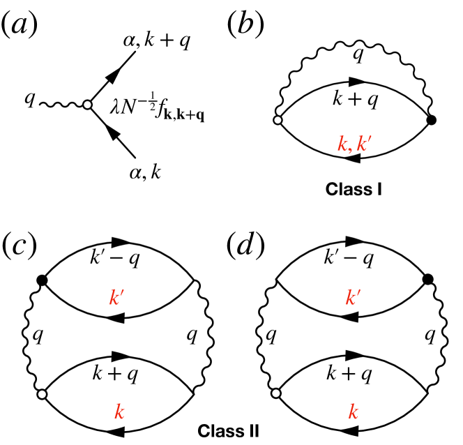
Figure 1: (a) Diagrammatic representation of $\dot{n}_{\alpha\mathbf{k}}(\Omega)$. The open/closed circles denote inflow/outflow of an external frequency $\Omega$. The vertex function changes sign depending on if the $\alpha\mathbf{k}$ state is an initial (final) state of the scattering. (b-d) Two class of diagrams for the memory matrix $M_{\alpha\mathbf{k},\beta\mathbf{k^{\prime}}}\left(\Omega\right)$. The red colored labels correspond to external momenta $\mathbf{k}$ and $\mathbf{k^{\prime}}$. For convenience we omitted the flavor index on the fermionic Green’s functions, and the summation over internal frequencies is implicit.

At temperatures $T\gg\Omega_{\text{NFL}}$, we compute $M_{\mathbf{\alpha k},\mathbf{\beta k}^{\prime}}$ in a $1/N$ expansion. Depending on the placement of the two momentum states $\mathbf{k}$ and $\mathbf{k}^{\prime}$, there are two classes of Feynman diagrams that contribute to leading order, as illustrated in Figure 1(b-d). In these diagrams, the nematic propagator includes the one-loop self energy: $D^{-1}(\mathbf{q},i\nu_{n})=D_{0}^{-1}-\Pi(\mathbf{q},i\nu_{n})$, where

$$\Pi(\mathbf{q},i\nu_{n})=-\lambda^{2}T\sum_{\omega_{m},\mathbf{k}}f_{\mathbf{k},\mathbf{k}+\mathbf{q}}^{2}G_{0}(\mathbf{k},i\omega_{m})G_{0}(\mathbf{k}+\mathbf{q},i\omega_{m}+i\nu_{n}),$$ (6)

whereas the fermion propagators $G_{0}(\mathbf{k},i\omega_{n})=1/(i\omega_{n}-\varepsilon_{\mathbf{k}})$ are the bare ones. At low frequencies, we write $D^{-1}(\mathbf{q},i\nu_{n})=r_{\mathbf{q}}+\gamma_{\mathbf{q}}|\nu_{n}|$, where $r_{\mathbf{q}}$ includes the renormalization effects from $\Pi(\mathbf{q},i\nu_{n}=0)$, and $\gamma_{\mathbf{q}}=\pi\lambda^{2}\sum_{\mathbf{k}}f_{\mathbf{k},\mathbf{k}+\mathbf{q}}^{2}\delta(\varepsilon_{\mathbf{k}})\delta(\varepsilon_{\mathbf{k}+\mathbf{q}})$.

A detailed derivation of the expressions corresponding to these Feynamn diagrams is presented in Appendix A.2. For class I [Fig. 1(b)], we obtain:

$$\begin{split}M_{\alpha\mathbf{k},\beta\mathbf{k^{\prime}}}^{(1)}(i\Omega_{n})=&\delta_{\alpha\beta}\frac{\lambda^{2}T}{N\Omega_{n}}\sum_{\mathbf{q},\nu_{n}}D_{\mathbf{q},\nu_{n}+\Omega_{n}}\\ \times&\sum_{\zeta=\pm 1}\left(\delta_{\mathbf{k}^{\prime}-\mathbf{k},\zeta\mathbf{q}}-\delta_{\mathbf{kk}^{\prime}}\right)f_{\mathbf{k},\mathbf{k+\zeta q}}^{2}R_{\mathbf{k},\mathbf{k+\zeta q},\zeta\nu_{n}}\end{split}$$

where $R_{\mathbf{k},\mathbf{k+q},\nu_{n}}$ is the polarization bubble summed over the internal fermionic Matsubara frequencies:

$$R_{\mathbf{k},\mathbf{k+q},\nu_{n}}=\frac{n_{F}\left(\varepsilon_{\mathbf{k+q}}\right)-n_{F}\left(\varepsilon_{\mathbf{k}}\right)}{\varepsilon_{\mathbf{k}}-\varepsilon_{\mathbf{k+q}}+i\nu_{n}}.$$ (7)

Here, $n_{F}(\varepsilon)$ is the Fermi function. Similarly, the expression for class II diagrams is

$$\begin{split}M_{\alpha\mathbf{k},\beta\mathbf{k^{\prime}}}^{(2)}(i\Omega_{n})&=-\frac{\lambda^{4}T}{N^{2}\Omega_{n}}\sum_{\mathbf{q},\nu_{n}}D_{\mathbf{q},\nu_{n}}D_{\mathbf{q},\nu_{n}+\Omega_{n}}\\ &\times\sum_{\zeta\zeta^{\prime}=\pm 1}\zeta\zeta^{\prime}f_{\mathbf{k},\mathbf{k}+\zeta\mathbf{q}}^{2}f_{\mathbf{k}^{\prime},\mathbf{k}^{\prime}+\zeta^{\prime}\mathbf{q}}^{2}R_{\mathbf{k},\mathbf{k}+\zeta\mathbf{q},\zeta\nu_{n}}\\ &\times\left[R_{\mathbf{k}^{\prime},\mathbf{k}^{\prime}+\zeta^{\prime}\mathbf{q},\zeta^{\prime}\nu_{n}}-R_{\mathbf{k}^{\prime},\mathbf{k}^{\prime}+\zeta^{\prime}\mathbf{q},\zeta^{\prime}\left(\nu_{n}+\Omega_{n}\right)}\right]\end{split}$$ (8)

For simplicity, we have omitted the static part $G_{\dot{n}_{\alpha\mathbf{k}}\dot{n}_{\beta\mathbf{k}^{\prime}}}^{R}(0)$ in the expressions. However, they are always subtracted in later calculations. The memory matrix are expressed in Matsubara frequencies. To obtain real-time dynamics, we perform an analytic continuation $i\Omega_{n}\rightarrow\Omega+i\delta$.

At high frequencies, these terms in the memory matrix reproduce the standard Feynman diagrams describing contributions to optical conductivity, namely Maki-Thompson (MT), Density of States (DOS) and Aslamazov-Larkin (AL) diagrams. This is shown in Appendix G. In particular, MT and DOS diagrams combine to give class I diagram, corresponding to the $\delta_{\mathbf{k^{\prime}-k},\mathbf{q}}$ and $\delta_{\mathbf{kk^{\prime}}}$ terms respectively. AL is equivalent to class II diagrams.

In the dc limit, our memory matrix approach is equivalent to the quantum Boltzmann equation discussed in the Kadanoff-Baym-Keldysh framework Kadanoff and Baym (1962); Rammer and Smith (1986); Kamenev (2011), and that conservation laws are explicitly built in. We discuss the conservation laws and their implications for the structure of the memory matrix. One can easily check that $\sum_{\alpha\mathbf{k}}M_{\alpha\mathbf{k},\beta\mathbf{k^{\prime}}}=0$, corresponding to electron number conservation. Note that the two class of diagrams separately conserve particle number. In Appendix B we show that in the absence of impurity and umklapp scattering, the total electronic momentum is conserved: $\sum_{\alpha\mathbf{k}}\mathbf{k}M_{\alpha\mathbf{k},\beta\mathbf{k^{\prime}}}=0$. Momentum conservation crucially relies on the fact that the nematic fluctuations gain their dynamics only as a result of their coupling to the electrons. As a result, they do not act as a “sink” for the total electronic momentum. It is worth noting that momentum is conserved only when the two classes of diagrams are combined, but not for each class separately.

III.2 Low temperature and dc limit

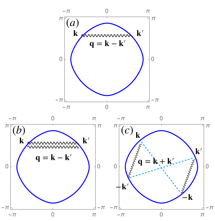
Figure 2: Three types of scattering processes when the relevant momentum states are in the vicinity of the Fermi surface. (a) class I diagram describes direct scattering between $\mathbf{k}$ and $\mathbf{k^{\prime}}$ mediated by exchanging an nematic boson $\phi_{\mathbf{q}}$ with $\mathbf{q}=\mathbf{k^{\prime}-k}$. (b) and (c) are two-electron scatterings mediated by two nematic bosons, described by class I diagram. (b) describes the momentum exchange scattering, where two electrons with momentum $\mathbf{k}$ and $\mathbf{k^{\prime}}$ exchange their momentum. (c) describes the head-on scattering, where two electrons located at $\mathbf{k}$ and $\mathbf{-k}$ are scattered into $\mathbf{k^{\prime}}$ and $-\mathbf{k^{\prime}}$.

At low temperatures compared to the Fermi energy $\varepsilon_{F}$, the dominant scattering processes occur in the vicinity of the Fermi surface. For two given momentum states on the Fermi surface $\mathbf{k}$ and $\mathbf{k^{\prime}}$, there are three types of processes described by class I and class II diagrams, as depicted in Figure 2. Class I diagram describes the direct scattering between $\mathbf{k}$ and $\mathbf{k^{\prime}}$ states mediated by a nematic boson with momentum $\mathbf{q}=\mathbf{k^{\prime}}-\mathbf{k}$. Class II diagram describes two-electron scattering which involves two additional momentum states $\mathbf{k+q}$ and $\mathbf{k^{\prime}\pm q}$. We consider a convex Fermi surface with inversion symmetry . Due to the one-dimensionality of the Fermi surface, there are only two allowed scattering processes which satisfy that all four momentum states are on the Fermi surface, as shown in Figs. 2(b) and (c). Panel (b) describes momentum exchange scattering, with $\mathbf{q=\mathbf{k^{\prime}-k}}$. Here two electrons at $\mathbf{k}$ and $\mathbf{k^{\prime}}$ are scattered into each other. (c) is a head-on collision, with $\mathbf{q=k+k^{\prime}}$. Here two electrons initially at $\mathbf{k}$ and $\mathbf{-k}$ are scattered into $\mathbf{k^{\prime}}$ and $-\mathbf{k^{\prime}}$.

Since the dominant contribution to the memory matrix comes from the vicinity of the Fermi surface, we can approximate $R$ defined in Eq. (7) as follows:

$$R_{\mathbf{k},\mathbf{k^{\prime}+q},\nu_{n}}\approx-\pi|\nu_{n}|\delta\left(\varepsilon_{\mathbf{k}}\right)\delta\left(\varepsilon_{\mathbf{k+q}}\right).$$ (9)

This approximation is justified in Appendix C. After performing summation over the bosonic Matsubara frequencies, we can simplify the memory matrix to be:

$$\begin{split}M_{\alpha\mathbf{k},\beta\mathbf{k^{\prime}}}^{(1)}&=\delta_{\alpha\alpha^{\prime}}\frac{2\pi\lambda^{2}}{N}\sum_{\mathbf{q}}V_{\mathbf{q}}(T)\left(\delta_{\mathbf{kk}^{\prime}}-\delta_{\mathbf{k}^{\prime}-\mathbf{k},\mathbf{q}}\right)\\ &\times f_{\mathbf{k},\mathbf{k+q}}^{2}\delta\left(\varepsilon_{\mathbf{k}}\right)\delta\left(\varepsilon_{\mathbf{k+q}}\right),\end{split}$$ (10)

and

$$\begin{split}M_{\alpha\mathbf{k},\beta\mathbf{k^{\prime}}}^{(2)}&=-\frac{2\pi^{2}\lambda^{4}}{N^{2}}\sum_{\mathbf{q}}\frac{V_{\mathbf{q}}(T)}{\gamma_{\mathbf{q}}}f_{\mathbf{k},\mathbf{k}+\mathbf{q}}^{2}\delta\left(\varepsilon_{\mathbf{k}}\right)\delta\left(\varepsilon_{\mathbf{k+q}}\right)\\ &\times\sum_{\zeta^{\prime}=\pm 1}\zeta^{\prime}f_{\mathbf{k}^{\prime},\mathbf{k}^{\prime}+\zeta^{\prime}\mathbf{q}}^{2}\delta\left(\varepsilon_{\mathbf{k^{\prime}}}\right)\delta\left(\varepsilon_{\mathbf{k^{\prime}+\zeta^{\prime}q}}\right),\end{split}$$ (11)

where we have defined

$$V_{\mathbf{q}}(T)\equiv\int_{-\infty}^{\infty}\frac{\mathrm{d}\omega}{\pi}\omega\text{Im}D_{\mathbf{q},\omega}\left(-\frac{\partial n_{B}(\omega)}{\partial\omega}\right),$$ (12)

The imaginary part of the nematic propagator is $\text{Im}D_{\mathbf{q},\omega}=\gamma_{\mathbf{q}}\omega/(r_{\mathbf{q}}^{2}+\gamma_{\mathbf{q}}^{2}\omega^{2})$, and $n_{B}(\omega)$ is the Bose-Einstein distribution function.

In the case of a single convex Fermi sheet with no umklapp scattering, there are additional conservation laws that emerge at low temperature. In particular, all the odd-parity deformations of the Fermi surface are quasi-conserved, in the sense that the lifetimes of these modes are parametrically larger than those of the even-parity modes Gurzhi et al. (1995); Maslov et al. (2011); Ledwith et al. (2017). This is because the only possible collisions on a one dimensional convex Fermi surface are either forward scattering or head-on collisions, and in both cases the odd moments of the distribution function do not change. These approximate conservation laws are manifest in the structure of the memory matrix, as demonstrated in Appendix D.

IV Current relaxation mechanisms and dc resistivity

We now turn to discuss how the quantum critical fluctuations manifest themselves in the temperature dependence of the dc resistivity, $\rho(T)$, through different current relaxation mechanisms. In a metal with a generic electron density, the electrical current cannot relax completely (and hence $\rho=0$) unless momentum conservation is violated. Having a non-zero resistivity therefore relies crucially on the momentum relaxation mechanism, either through impurity or umklapp scattering. In the special case of a compensated metal with an equal density of electrons and holes, the resistivity is finite even if the total momentum is conserved.

We note that in our calculation, the temperature dependence comes from the scattering rates, encoded in the memory matrix. The thermodynamic susceptibilities, $\chi_{J_{x},\alpha\mathbf{k}}$ and $\chi_{\alpha\mathbf{k},\beta\mathbf{k^{\prime}}}$, defined in Eq. (4), can be regarded as temperature independent. While this is not true for the Ising-nematic (B_1g) channel, where the thermodynamic susceptibility diverges at the QCP, this divergence does not affect the transport properties, since the current operator (as well as any other odd-partiy deformation of the Fermi surface) is orthogonal to the nematic order parameter.

We will present our results for $\rho(T)$ in dimensionless units. The temperature is rescaled by the energy scale set by the Landau damping term: $\Omega_{L}\equiv\varepsilon_{F}^{2}\lambda^{-2}$. As we discuss in Appendix A.2, the natural scale for the resistivity in our problem is $\rho_{L}\equiv\frac{\hbar}{e^{2}}\frac{\lambda^{4}}{\varepsilon_{F}^{2}}\frac{1}{N^{2}}$. Note that in the large-$N$ or weak coupling limits, where our approach is valid, $\rho_{L}$ is always much smaller than the quantum of resistance $\hbar/e^{2}$.

IV.1 Impurity scattering

We consider quenched disorder, modeled by a random potential: $H_{\text{imp}}=\frac{1}{\sqrt{N}}\sum_{\alpha\mathbf{r}}V_{\text{imp}}(\mathbf{r})c_{\alpha\mathbf{r}}^{\dagger}c_{\alpha\mathbf{r}}$, where $V_{\text{imp}}(\mathbf{r})$ has the following properties: $\overline{V_{\text{imp}}(\mathbf{r})}=0$ and $\overline{V_{\text{imp}}(\mathbf{r})V_{\text{imp}}(\mathbf{r^{\prime}})}=g_{\text{imp}}^{2}\delta\left(\mathbf{r-r^{\prime}}\right)$, where $\overline{\cdots}$ denotes disorder averaging. The time-derivative of the electron occupation number is given by $(\dot{n}_{\alpha\mathbf{k}})_{\text{imp}}=\frac{i}{\sqrt{N}}\sum_{\mathbf{q}}V_{\text{imp},\mathbf{q}}\left(c_{\alpha\mathbf{k}}^{\dagger}c_{\alpha\mathbf{k+q}}-c_{\alpha\mathbf{k-q}}^{\dagger}c_{\alpha\mathbf{k}}\right)$. As a result, for weak disorder strength, the leading correction to the memory matrix is given by

$$\begin{split}M_{\alpha\mathbf{k},\beta\mathbf{k^{\prime}}}^{\text{imp}}(i\Omega_{n})&=\delta_{\alpha\beta}\frac{1}{N\Omega_{n}}\sum_{\mathbf{q},i\nu_{n}}D_{\mathbf{q},\nu_{n}}^{\text{imp}}\sum_{\zeta=\pm 1}f_{\mathbf{k},\mathbf{k+\zeta q}}^{2}\\ &\times\left(\delta_{\mathbf{k}^{\prime}-\mathbf{k},\zeta\mathbf{q}}-\delta_{\mathbf{kk}^{\prime}}\right)R_{\mathbf{k},\mathbf{k+\zeta q},\zeta\nu_{n}+\zeta\Omega_{n},}\end{split}$$ (13)

where the correlator of the disorder potential is static and momentum-independent, i.e., $D_{\mathbf{q},\nu_{n}}^{\text{imp}}=g_{\text{imp}}^{2}\delta_{\nu_{n},0}$. To leading order in impurity strength, we neglect the cross-terms involving both impurity and quantum critical scattering . At low temperatures, $T\ll\varepsilon_{F}$, we project the processes onto the Fermi surface, and approximate $R(\mathbf{k},\mathbf{k+q},i\Omega_{n})\approx-\pi|\Omega_{n}|\delta\left(\varepsilon_{\mathbf{k}}\right)\delta\left(\varepsilon_{\mathbf{k+q}}\right)$. As a result, in the dc limit,

$$M_{\alpha\mathbf{k},\beta\mathbf{k^{\prime}}}^{\text{imp}}=\delta_{\alpha\beta}\frac{2\pi g_{\text{imp}}^{2}}{N}\sum_{\mathbf{q}}\left(\delta_{\mathbf{kk^{\prime}}}-\delta_{\mathbf{k^{\prime}-k,q}}\right)\delta\left(\varepsilon_{\mathbf{k}}\right)\delta\left(\varepsilon_{\mathbf{k+q}}\right).$$ (14)

One can verify that momentum is no longer conserved under impurity scattering, by observing that

$$\sum_{\alpha\mathbf{k}}\mathbf{k}M_{\alpha\mathbf{k},\beta\mathbf{k^{\prime}}}^{\text{imp}}=-2\pi g_{\text{imp}}^{2}\sum_{\mathbf{q}}\mathbf{q}\delta\left(\varepsilon_{\mathbf{k}^{\prime}}\right)\delta\left(\varepsilon_{\mathbf{k^{\prime}+q}}\right).$$ (15)

This expression does not vanish for a general value of $\mathbf{k^{\prime}}$, due to the asymmetry of momentum states $\mathbf{k^{\prime}\pm q}$.

We first show that when there is only a single convex electron Fermi surface, quantum critical scattering does not contribute to the dc resistivity within our lowest-order approximation in $T/\varepsilon_{F}$. In this case, $\rho\approx\rho_{0}\propto g^{2}\nu_{F}$ coming from impurity scattering, where $\nu_{F}$ is the density of states at the Fermi level. To see this, we work in the basis of Fermi surface harmonics, $e^{in\theta_{\mathbf{k}}}$, where $\theta_{\mathbf{k}}$ is the angle between a point $\mathbf{k}$ on the Fermi surface and the $x$ axis. Since our problem is inversion-symmetric on average, $M_{\alpha n,\beta m}^{\text{imp}}$ is non zero only if $m$ and $n$ have the same parity. Electron-electron scattering on a single, convex Fermi surface conserves all the odd-parity modes Gurzhi et al. (1995); Maslov et al. (2011); Ledwith et al. (2017) (See Appendix D). Since the electrical current is parity-odd, it is completely decoupled from the quantum critical scattering to lowest order in $T/\varepsilon_{F}$. Hence, to lowest order in $T/\varepsilon_{F}$, $\rho$ is temperature independent. Scattering processes away from the Fermi surface can give rise to $\rho(T)\sim T^{2+\alpha},$ with $\alpha=4/3$, as argued in Ref. Maslov et al. (2011).

Next, we study the case of multiple Fermi sheets. Different sheets generically have different energy dispersions and are separated in momentum space. The small-momentum nematic fluctuations induces intra-sheet scattering, while impurity scattering can be either intra- or inter-sheet. We write the electrical current operator as $\mathbf{J}=\sum_{i\mathbf{k}}\mathbf{v}_{i,\mathbf{k}}c_{i,\mathbf{k}}^{\dagger}c_{i\mathbf{k}}$, where $i$ is the sheet index. Due to differences in the Fermi velocities in each Fermi sheet, the current is not conserved by nematic scattering (unlike total momentum). As a result, the resistivity acquires a temperature-dependent correction $\sim T^{\alpha}$, whose exponent is determined by the decay of odd-parity modes on the Fermi surface. Scaling arguments suggest that nematic contrinbution to the current decay rate scales as $\bar{q}^{2}\tau_{\text{sp}}^{-1}$, where $\bar{q}\sim T^{1/3}$ is the typical momentum transfer following quantum critical scaling, and $\tau_{\text{sp}}^{-1}\sim T^{2/3}$ is the single-electron decay rate. As a result, for a multi-band system subject to impurity scattering, we expect that $\rho-\rho_{0}\propto T^{4/3}$ .

In Figure 3, we present a numerical calculation of $\rho(T)$ for system with either a single Fermi surface or multiple Fermi sheets, supporting the scaling argument discussed above. More details of the numerical procedure are given in Appendix J. In the single Fermi surface case, the resistivity is completely temperature-independent; we expect that inclusion of scattering processes away from the Fermi surface will give rise to a weak temperature dependence. In the multi-Fermi sheet case, we find a substantial temperature dependence. In panel (b) we show$\mathrm{d}\ln\left(\rho-\rho_{0}\right)/\mathrm{d}\ln T$ as a function of $T$ for the multi-sheet case. At low temperature, the exponent approaches $4/3$, as expected from the qualitative analysis above. However, at intermediate temperatures, the exponent drifts below $4/3$ and can even exhibit sublinear behavior. The cause of the drifting exponent will be discussed in Sec. IV.4.

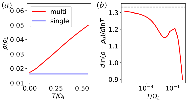
Figure 3: (a) Resistivity due to impurity scattering for a system with a single Fermi surface (blue) and multiple Fermi sheets (red) cases. In (b) we plot $d\ln\left(\rho-\rho_{0}\right)/d\ln T$ for multi-sheet case to extract the power-law dependence on temperature. The dashed line marks the value $4/3$. The dispersion used for one-band case is $\varepsilon_{\mathbf{k}}=-2t\left(\cos k_{x}+\cos k_{y}\right)-4t^{\prime}\cos k_{x}\cos k_{y}-\mu$ , with $t=1$, $t^{\prime}=-0.3$ and $\mu=-1$. In the multi-sheet case, we used three circularly-shaped Fermi pockets of equal size, with two electron-like and one hole-like dispersions. Impurity scattering strength is taken to be $g_{\text{imp}}=0.02\varepsilon_{F}$. The nematic-electronic coupling strength is $\lambda^{2}\approx 0.83\varepsilon_{F}$. The Fermi energy is defined as $\varepsilon_{F}=\langle v_{F}k_{F}\rangle_{\text{FS}}$.

IV.2 Umklapp scattering

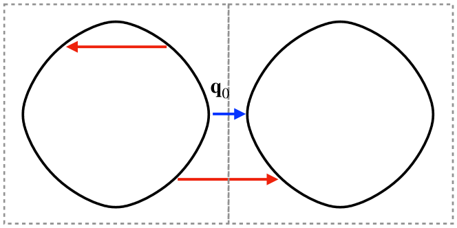
Figure 4: Two-particle collision involving a Umklapp process. One of the final states is a different Brillouin zone. Therefore, the total momentum changes by the crystal momentum $\mathbf{G}$. $\mathbf{q}_{0}$ is the minimal momentum transfer in an umklapp scattering event.

In the presence of an underlying lattice, the electronic momentum is only conserved up to a reciprocal lattice vector $\mathbf{G}$. In an umklapp scattering process, two of the initial states and one of the final states are on the Fermi surface in the first Brillouin zone, while the other final state is in a neighboring Brollouin zone. An umklapp scattering process on the Fermi surface involves a minimum momentum transfer $\mathbf{q}_{0}$ that depends on the geometry of the Fermi surface, as illustrated in Figure 4. Since the critical nematic fluctuations carry small momentum, they cannot induce umklapp scattering at asymptotically low temperatures. Therefore, below a characteristic temperature $T_{0}$ that depends on $\mathbf{q}_{0}$, we expect the dc transport to be governed by non-critical fluctuations. For $T\ll T_{0}$, the Fermi liquid behavior $\rho(T)\sim T^{2}$ behavior should be recovered Maslov et al. (2011). On scaling grounds, we expect $T_{0}\sim|\mathbf{q}_{0}|^{z}$, where $z$ is the dynamical critical exponent of the transition. At temperatures $T>T_{0}$ , there are two main factors determining the transport behavior: (1) As the typical wavevector for critical fluctuations $|\mathbf{q}|\sim T^{1/z}>|\mathbf{q}_{0}|$, critical fluctuations contribute to umklapp scattering and directly modify the dc transport properties. (2) The umklapp processes also modify the spectrum of the nematic critical fluctuations. In particular, they modify the coefficient $\gamma_{\mathbf{q}}$ of the Landau damping term in the bosonic self-energy, which depends on the angle between the Fermi velocities at the points $\mathbf{k}$ and $\mathbf{k}+\mathbf{q}$ on the Fermi surface. This can lead to a breakdown of the $z=3$ quantum critical scaling, which relies on the relation $\gamma_{\mathbf{q}}\sim 1/|\mathbf{q}|$.

We study $\rho(T)$ for a model with a generic, large Fermi surface, similar to the one shown in Fig. 4. This is done by numerically computing the memory matrix from Eqs. (10,11), including the effects of umklapp scattering, and inverting it to obtain the dc conductivity according to Eq. (4). In Fig. 5(a) and (c), we present $\rho(T)$ at and away from the Ising-nematic QCP, with a nematic correlation length $\xi^{-2}(T)=T+r-r_{c}$. Here, we assume that the at $r=r_{c}$, there is a “thermal mass” assumed to be proportional to $T$. The model parameters, listed in the caption of Fig. 5, are chosen to be similar to the ones used in the quantum Monte Carlo simulations in Ref. Schattner et al. (2016). Figure 5(b) shows $d\ln\rho/d\ln T$ as a function of $T$ and $r-r_{c}$. As expected, at sufficiently low temperatures, $\rho\sim T^{2}$. At higher temperature, $d\ln\rho/d\ln T$ decreases, becoming sublinear at temperatures of the order of $\Omega_{L}$. Defining $T_{0}$ as the temperature where $d\ln\rho/d\ln T=1.8$, we find that at the QCP, $T_{0}\propto|\mathbf{q}_{0}|^{3}$ [Fig. 5(d)]. Away from the QCP, the crossover to $T^{2}$ occurs at higher temperatures, and $T_{0}$ scales linearly with the distance to the QCP $r$.

Although for $r=r_{c}$ and $T>T_{0}$, there is a temperature window where $\rho(T)$ appears to be approximately linear (Fig. 5c), it is important to note that $d\ln\rho/d\ln T$ actually changes continuously in this regime. It is also worth noting that the dc resistivity obtained in our calculation reproduces many of the qualitative features observed in the QMC simulations of Ref. Schattner et al. (2016), including the broad quasi-linear regime near the QCP, and the gradual change of the slope of $\rho(T)$ as $r$ is tuned away from the QCP.

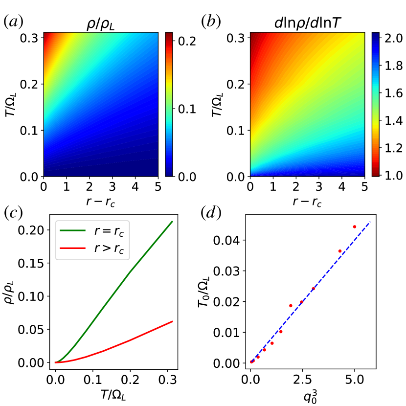
Figure 5: (a) Resistivity from umklapp scattering at and away near an Ising-nematic QCP, as a function of $r-r_{c}$ and $T$. Here, we use the same band dispersion studied for the single-band case for impurity scattering (see caption of Fig. 3). The coupling strength $\lambda^{2}=1.88\varepsilon_{F}$. (b) $d\ln\rho/d\ln T$ as a function of $r-r_{c}$ and $T$. (c) Temperature cuts at the QCP (green) and in the disordered state ($r>r_{c}$, red). (d) Crossover temperature to Fermi-liquid $T^{2}$ behavior as a function of the umklapp threshold wavevector $|\mathbf{q}_{0}|^{3}$. $\mathbf{q}_{0}$ was varied by changing the chemical potential $\mu$. We define $T_{0}$ as the temperature where $d\ln\rho/d\ln T=1.8$.

IV.3 Compensated metal

The mechanisms for current dissipation discussed so far rely on breaking the conservation of total electron momentum, either by impurity or by umklapp scattering. It is well-known that in a compensated metal with equal number of electron and hole-like charge carriers, electron-electron interactions alone can lead to a finite electrical resistivity, even in the absence of momentum relaxation (Baber and Mott, 1937). This is because scattering events between electrons and holes can relax the current, despite the fact that momentum is conserved. In a compensated metal, the electrical current and the total electronic momentum are orthogonal to each other: $\chi_{\mathbf{JP}}=0$, and the current dissipation is driven by relaxation of other odd-parity modes of the Fermi surface. For completeness, this result is re-derived in Appendix H.

Several of the iron-based superconductors known for exhibiting non-Fermi liquid transport, such as $\mathrm{FeSe_{1-x}S_{x}}$ Coldea and Watson (2018) and $\mathrm{BaFe_{2}(As_{1-x}P_{x})_{2}}$ Kasahara et al. (2010), are isovalently doped. These systems have multiple small Fermi surfaces (pockets) that are of either electron or hole character, with an equal density of electron and hole carriers. It is reasonable to assume that such materials are not far from being a compensated metal, and that normal electron-hole scattering mediated by quantum critical fluctuations plays an important role in their transport behavior.

In this Section, we study the temperature dependence of dc resistivity for a compensated metal near a nematic quantum critical point. Motivated by the case of the iron-based superconductors, we focus on the case where the electron and hole pockets are much smaller than the Brillouin zone size, such that umklapp scattering is negligible. Since the nematic critical fluctuations are centered at small momenta, we assume that they cannot scatter electrons from one pocket to the other. The Hamiltonian is given by

$$H=\sum_{i=1}^{n}\left(\sum_{\mathbf{k}}\varepsilon_{i\mathbf{k}}c_{i\mathbf{k}}^{\dagger}c_{i\mathbf{k}}+\lambda\sum_{\mathbf{kq}}\phi_{\mathbf{q}}f_{i,\mathbf{k,k+q}}c_{i\mathbf{k+q}}^{\dagger}c_{i\mathbf{k}}\right),$$ (16)

where $i=1,\dots,n$ is the pocket index, and the pocket dispersions $\varepsilon_{i\mathbf{k}}$ are assumed to be such that the total area enclosed by the electron-like pockets is equal to that of the hole-like pockets. $f_{i,\mathbf{k},\mathbf{k}+\mathbf{q}}$ is the Ising-nematic form factor of the $i$th pocket, centered at wavevector $\mathbf{Q}_{i}$. Importantly, depending on the position of the Fermi pocket in the Brillouin zone, the form factor may or may not contain “cold spots” – points on the Fermi pocket where the form factor vanishes. For example, a pocket centered at the $\Gamma$ point [$\mathbf{Q}_{i}=(0,0)$] has cold spots where the diagonals $k_{x}=\pm k_{y}$ intersect the Fermi surface. In contrast, a pocket at the $X$ or $Y$ points [$\mathbf{Q}_{i}=(\pi,0)$ or $(0,\pi)$, respectively] does not have any symmetry-imposed cold spots. The band structures of most of the iron-based superconductors contain pockets centered at both the $\Gamma$, $X$, and $Y$ points (in the one Fe per unit cell scheme). As we shall see below, the presence of cold spots on the Fermi pockets, and whether they occur on all or only some of the pockets, changes qualitatively transport behavior at low temperature.

We study $\rho(T)$ in four different scenarios: in a clean system where (1) all the pockets have cold spots, (2) the hole pockets have cold spots but the electron pockets do not, (3) no pockets have cold spots, and (4) a disordered system where all the pockets have cold spots. For simplicity, we considered a model with two circular pockets with identical radii, one electron-like and one hole-like. We do not expect the results to change qualitatively for pockets of a general shape, as long as the system is perfectly compensated (see Appendix I). The results are summarized in Fig. 6. In the case when cold spots are absent or if there is weak impurity scattering (Fig. 6 green and magenta lines), $\rho(T)-\rho_{0}\propto T^{4/3}$, which is the naive quantum critical scaling exponent discussed previously Löhneysen et al. (2007); Maslov et al. (2011). However, in a clean compensated metal with cold spots on one or both of the Fermi pockets, the asymptotic low-temperature behavior is different. When cold spots are present on some (but not all) of the pockets, $\rho\sim T^{5/3}$ (blue curve), whereas when cold spots are present on all the pockets, $\rho\sim T^{2}$ (red curve).

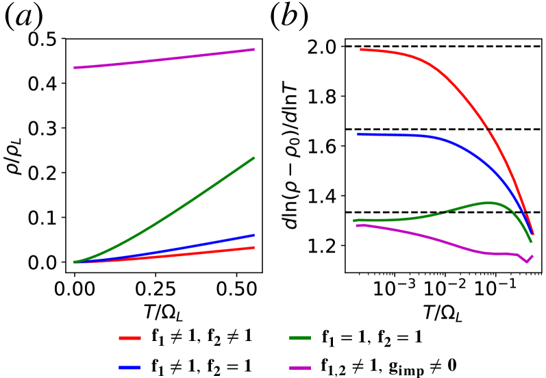
Figure 6: $\rho(T)$ and the log-derivative plot at the QCP in a perfectly compensated metal with different arrangements of cold spots on the Fermi pockets. The model consists of two circular pockets with equal radii, one electron-like and one hole-like. The nematic form factor is either taken to be $\cos 2\theta_{\mathbf{k}}$ when the corresponding pocket has cold spots, or unity for the case with no cold spots. The coupling constant is $\lambda^{2}\approx 0.84\varepsilon_{F}$. Red curve: both pockets have cold spots along the diagonals. Blue curve: cold spots on the hole pocket, but not the electron pocket. Green curve: neither pocket has cold spots. Magenta curve: both pockets have cold spots, but also subject to impurity scattering of strength $g_{\text{imp}}\approx 0.1\varepsilon_{F}$. The black dashed lines in (b) correspond to exponents of $4/3$, $5/3$ and $2$.

To understand the origin of the strong sensitivity of the low-temperature transport behavior to the presence of cold spots, we examine the non-equibrium distribution function in the presence of a current. It is convenient to parametrize the distribution function $\delta n_{i\mathbf{k}}$ in terms of another function $\Phi_{i\mathbf{k}}$ such that $\delta n_{\mathbf{k}}=\left[-\partial_{\varepsilon_{i\mathbf{k}}}n_{F}(\varepsilon_{i\mathbf{k}})\right]\Phi_{i\mathbf{k}}E_{x}$, where $i$ is the band index, $\mathbf{k}$ is a point on the Fermi surface and $\mathbf{E}=E_{x}\hat{x}$ is the electric field applied along the $x$ axis. $\Phi_{i\mathbf{k}}$ can be computed from the memory matrix according to: $\Phi_{i\mathbf{k}}=\left(M^{-1}\right)_{i\mathbf{k},j\mathbf{k^{\prime}}}\chi_{j\mathbf{k^{\prime}},J_{x}}$. More details on relation between our memory matrix approach and the non-equilibrium distribution function are given in Appendix F. Fig. 7(a) shows the clean case without hot spots. In this case, $\Phi_{1\theta_{\mathbf{k}}}=-\Phi_{2\theta_{\mathbf{k}}}=\cos\theta_{\mathbf{k}}$. However, when cold spots are present on at least one Fermi pocket, the distribution function on both pockets changes dramatically, as seen in Fig. 7(b) and (c). In this case, the distribution function is nearly constant on different quadrants of the Fermi surface, bounded by the cold spots. In the presence of disorder, the distribution function becomes more regular and approaches a cosine at low temperatures, as seen in Fig. 7(d).

Figure 7: The function $\Phi_{i,\theta_{\mathbf{k}}}\propto\delta n_{i,\theta_{\mathbf{k}}}$ on Fermi pocket $i=1,2$ in the presence of a current in the $x$ direction, for the same model as in Fig. 6. Here $\theta_{\mathbf{k}}$ is the angle measured with respect to the $x$-direction. The solid (dashed) curve is the distribution function on the electron (hole) pocket. The colors correspond to the same cases shown in Fig. 6. All four distribution functions are calculated at the same temperatures $T\approx 0.002\varepsilon_{F}$.

The shape of the non-equilibrium distribution function in the presence of cold spots can be understood qualitatively as follows: at low temperatures, the characteristic momentum transfer $q$ due to quantum critical scattering, $q\sim k_{F}\left(T/\Omega_{L}\right)^{1/3}$, is small. The scattering rate from a point $\mathbf{k}$ near one of the cold spots to a nearby point $\mathbf{k}+\mathbf{q}$ is suppressed by the nematic form factor. Therefore, the cold spots effectively cut the Fermi surface into four nearly-disconnected patches. The equilibration within each patch is much faster than the equilibration between patches (see Fig. 8). In this situation, the non-equilibrium distribution is nearly constant in each patch, and the bottleneck for current relaxation becomes the slow inter-patch scattering. As a result, the resistivity in the presence of cold spots is reduced than the resistivity with no cold spots. In Appendix I, we analyze the transport properties in the presence of cold spots, using a piecewise-constant distribution function of the form shown in Fig. 7(b,c) as a variational ansatz. We find that the power-law exponents observed in Figure 6 are exactly reproduced.

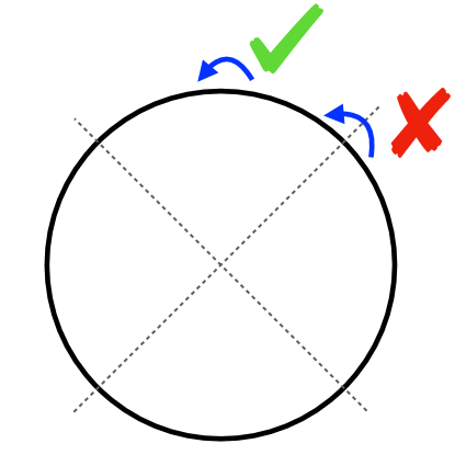
Figure 8: Electron scattering on the Fermi surface due to small wavevector nematic fluctuations. The intersection between the Fermi surface and the dashed lines are where the nematic form factor vanishes — the nematic “cold spots”. Small wavevector scattering across the cold spots are strongly suppressed by the nematic form factor.

IV.4 Quasi-elastic thermal fluctuations and intermediate temperature behavior

Having analyzed the asymptotic low-temperature behavior of the resistivity due to different scattering mechanisms, we turn to discuss the crossover behavior at higher temperatures. In particular, depending on microscopic parameters, there may be a regime where the temperature is comparable to or larger than the energy scale set by the Landau damping, $\Omega_{L}$, but still much smaller than the Fermi energy. Since $\Omega_{L}=\varepsilon_{F}^{2}/\lambda^{2}$, this regime is accessible within our model at strong coupling (or, equivalently, if the Fermi energy is small). Formally, the calculation in this regime can still be controlled in the large $N$ limit, as long as $T\gg\Omega_{\text{NFL}}$. As we shall now show, the resistivity is determined by quasi-elastic scattering of electrons off thermally excited nematic fluctuations. Depending on the evolution of the correlation length with temperature, this may lead to either $\rho\sim T$ or $\rho\sim\text{const.}$ in the crossover regime.

We begin by examining the temperature dependence of the scattering cross-section between electrons and nematic fluctuations, $V_{\mathbf{q}}(T)$ [see Eqs. (10–12)]. We write Eq. (12) as $V_{\mathbf{q}}(T)=\frac{1}{\gamma_{\mathbf{q}}}F\left(\frac{T}{\omega_{\mathbf{q}}}\right)$, where $\omega_{\mathbf{q}}\equiv r_{\mathbf{q}}\gamma_{\mathbf{q}}^{-1}$ (recall that the nematic propagator is written as $D_{\mathbf{q},\nu_{n}}^{-1}=r_{\mathbf{q}}+\gamma_{\mathbf{q}}|\nu_{n}|$) and

$$F\left(x\right)\equiv\frac{1}{x}\int_{-\infty}^{+\infty}\frac{\mathrm{d}u}{\pi}\frac{u^{2}}{1+u^{2}}\frac{1}{\sinh^{2}\left(\frac{u}{2x}\right)}.$$ (17)

$F\left(x\right)$ has the following asymptotic properties: for $x\ll 1$, $F(x)\approx\pi x^{2}/3$, whereas for $x\gg 1$, $F(x)\approx 4x$.

We can now estimate the resistivity in the regime $T\gg\Omega_{L}\sim\omega_{\mathbf{q}\sim k_{F}}$, that corresponds to $x\gg 1$ in Eq. (17). In this regime, the dominant contribution to $V_{\mathbf{q}}(T)$ is from energies $\omega\sim\omega_{\mathbf{q}}\ll T$, corresponding to quasi-elastic scattering of electrons off thermally excited nematic fluctuations. We focus on the case of a compensated metal, where momentum conservation does not limit the resistivity. At high temperatures, we do not expect the nematic form factor to have a strong effect on the results, and will henceforth neglect it. The resistivity can then be estimated by overlapping the memory matrix described by class I diagram with the current operator:

$$\rho(T)\propto\sum_{\mathbf{kk^{\prime}}}\left(\mathbf{v}_{\mathbf{k}}\cdot\mathbf{v}_{\mathbf{k^{\prime}}}\right)M_{\mathbf{kk^{\prime}}}^{(1)}\sim\int_{0}^{k_{F}}\mathrm{d}qq^{2}V_{\mathbf{q}}\left(T\right).$$ (18)

Placing both $\mathbf{k}$ and $\mathbf{k+q}$ on the Fermi surface (recall that we are still considering $T\ll\varepsilon_{F}$) constrains the allowed wave-vector $\mathbf{q}$ to a one-dimensional manifold. The first $q^{2}$ term in the integrand is the well-known transport factor that suppresses the contribution of small angle scattering. This factor arises from the term $\sum_{\mathbf{q,kk^{\prime}}}\left(\mathbf{v}_{\mathbf{k}}\cdot\mathbf{v}_{\mathbf{k^{\prime}}}\right)\left(\delta_{\mathbf{kk^{\prime}}}-\delta_{\mathbf{k^{\prime}-k,q}}\right)\sim\sum_{\mathbf{q,k}}\left(\mathbf{v}_{\mathbf{k}}-\mathbf{v}_{\mathbf{k+q}}\right)^{2}$ that appears when inserting Eq. (10) in Eq. (18).

When $T>\Omega_{L}$, nematic fluctuations with a large wavevector $q\sim k_{F}$ become thermally excited. From the discussion above [Eq. (17)], we find that in this regime $V_{\mathbf{q}}(T)\sim T/r_{\mathbf{q}}$, and hence

$$\rho(T)\propto T\int_{0}^{k_{F}}\mathrm{d}q\frac{q^{2}}{\xi^{-2}(T)+q^{2}}$$

where we have expressed $r_{\mathbf{q}}(T)=\xi^{-2}(T)+\mathbf{q}^{2}$. If $\xi\approx\xi_{0}$ is only weakly dependent on temperature, or if $\xi^{-1}\ll k_{F}$, then $\rho(T)\sim T$. In contrast, if $\xi^{-1}(T)\gg k_{F}$, then the behavior of $\rho(T)$ is determined by the temperature dependence of $\xi(T)$. For $\xi^{-2}\sim T$ (as was observed in the QMC simulations of Ref. Lederer et al. (2017), and experimentally in Ref. Böhmer and Meingast (2016)), $\rho(T)$ saturates to a constant at high temperature. In Figure 9, we illustrate both types of high temperature behavior for a compensated metal without cold spots, as discussed in the previous section.

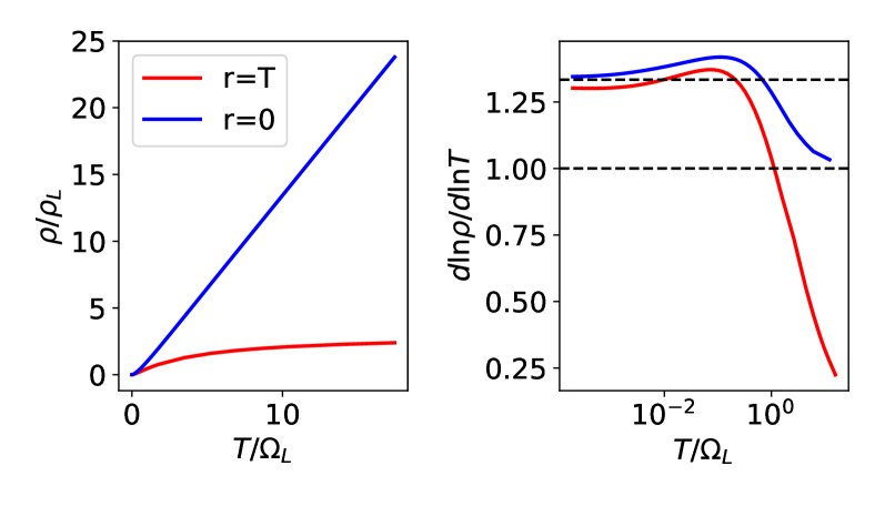
Figure 9: $\rho(T)$ in the high temperature regime $T>\Omega_{L}$, calculated for a compensated metal without cold spots. $r(T)\equiv\xi^{-2}(T)$ is the thermal mass for nematic fluctuations. The calculation assumes strong coupling $\lambda^{2}\gg\varepsilon_{F}$ and large fermion flavor $N$, so that $\Omega_{L}\ll\varepsilon_{F}$, and our memory matrix approach remains valid.

V Conclusion

In summary, we have developed a memory matrix approach to derive a kinetic equation applicable in a broad temperature regime near an Ising-nematic QCP. The formalism is applied to study the behavior of the dc resistivity in the vicinity of the QCP. The resistivity exhibits a rich behavior that depends on the dominant mechanism for current dissipation and on the structure of the Fermi surface.

We find several regimes where the resistivity is strongly affected by nematic critical fluctuations, despite their long–wavelength nature. As long as the Fermi surface is not very small compared to the size of the Brillouin zone, there is a broad temperature range where the resistivity is strongly enhanced near the QCP due to umklapp scattering; in this regime, the umklapp processes also modify the spectrum of the critical nematic fluctuations, and $z=3$ dynamical scaling does not hold. At asymptotically low temperatures, however, $z=3$ scaling is recovered, and $\rho\sim T^{2}$. In multi-band systems in the presence of impurities, $\rho-\rho_{0}\propto T^{4/3}$ down to the lowest temperatures, as anticipated from $z=3$ dynamical scaling. In a compensated metal with an equal density of electrons and holes, the quantum critical fluctuations can affect the resistivity even in the absence of impurities and at arbitrarily low temperatures. In this case we find that the dc resistivity is strongly affected by the presence of “cold spots” on the Fermi sheets, due to the symmetry of the nematic order parameter. In the clean limit, $\rho\sim T^{\alpha}$, where $\alpha=2$, $5/3$, or $4/3$, depending on whether there are cold spots on all the Fermi sheets, on some of the sheets, or on none, respectively.

It is important to note that we have assumed a purely electronic mechanism for the Ising-nematic QCP, and have neglected the effect of coupling to the lattice. This effect is known to change the properties of the QCP, quenching most of the long-wavelength nematic fluctuations and making the transition more mean-field like Zacharias et al. (2015); Karahasanovic and Schmalian (2016); Paul and Garst (2017). As a result, the effect of the critical fluctuations on the resistivity is suppressed, recovering Fermi liquid behavior $\rho-\rho_{0}\propto T^{2}$ at the lowest temperatures. The scale at which the crossover to Fermi liquid behavior occurs depends on the strength of the coupling to the lattice.

Our analysis can be extended straightforwardly to other metallic QCPs in $d=2$ dimensions that do not involve breaking of translational symmetry, such as ferromagnetic transitions. In the latter case, there are generically no cold spots on the Fermi surface.

The diversity of possible behaviors found in our study suggest that experiments in critical metals should be interpreted with great care. Nevertheless, it would be interesting to consider our results in the context of ongoing experiments Reiss et al. in $\mathrm{FeSe_{1-x}S_{x}}$, which is a compensated system that exhibits an apparent nematic QCP with no nearby magnetic phase.

Appendix A Memory matrix approach to transport properties

A.1 General formalism

In this section, we briefly review the memory matrix formalism and its application to transport. We then discuss the validity of the approach in the vicinity of a QCP.

We closely follow the discussion of the memory matrix approach in Ref. Hartnoll et al. (2018). To set up the formalism, we first define an inner product in the Hilbert space of operators. For two Hermitian operators $A$, $B$, the inner product is given by

$$(A|B)=T\int_{0}^{\beta}d\tau\left[\langle A(\tau)B\rangle-\langle A\rangle\langle B\rangle\right]\equiv T\chi_{AB}.$$ (19)

Here, $\chi_{AB}$ is a theormodynamic susceptibility relating the operators $A$ and $B$.

The Liouville “super operator” is defined as $\mathcal{L}=-[H,\cdot]$. The operators satisfy the Heiseberg equation of motion: $\dot{A}=i[H,A]=-i\mathcal{L}A$. We are interested in calculating a retarded correlation function of two operators, characterizing the response of the system. This can be done through the relation Hartnoll et al. (2018)

$$G_{AB}^{R}(t)\equiv i\Theta(t)\langle[A(t),B(0)]\rangle=-\frac{1}{T}\Theta(t)\partial_{t}C_{AB}(t),$$ (20)

where $C_{AB}(t)\equiv(A(t)|B)$. Fourier transforming both sides, we obtain

$$\widetilde{C}_{AB}(z)=\frac{T}{iz}\left[\tilde{G}_{AB}^{R}(z)-\tilde{G}_{AB}^{R}(0)\right],$$ (21)

where $\widetilde{C}_{AB}(z)\equiv\int_{0}^{\infty}e^{izt}C_{AB}(t)$, $z$ is a complex number in the upper half plane, and similarly for $\tilde{G}_{AB}^{R}(z)=\int_{0}^{\infty}e^{izt}G_{AB}^{R}(t)$. For example, the frequency-dependent conductivity can be written as

$$\sigma(\Omega)\equiv\frac{1}{i\Omega}\left[\tilde{G}_{J_{x}J_{x}}^{R}(\Omega)-\tilde{G}_{J_{x}J_{x}}^{R}(0)\right]=\frac{1}{T}\widetilde{C}_{J_{x}J_{x}}(z=\Omega+i0^{+}).$$ (22)

The key step in the memory matrix technique is to identify a set of slow (or nearly-conserved) operators, and project the dynamics onto these operators. We denote the set of slow operators by $|A_{\alpha})$. We assumne that the current is a linear combination of $|A_{\alpha})$’s. Then, to compute $\widetilde{C}_{J_{x}J_{x}}(z)$, it is sufficient to compute matrix elements of the resolvent (or Green’s function) $\hat{G}(z)=\frac{i}{z-\mathcal{L}}$ in the subspace of $|A_{\alpha})$. To do this, we define the projection operator

$$\hat{P}=\frac{1}{T}\sum_{\alpha,\beta}|A_{\alpha})(\chi^{-1})_{\alpha\beta}(A_{\beta}|$$ (23)

onto the slow subspace, and $\hat{Q}=1-\hat{P}$ is a projection onto the complementary subspace. The equation for the Green’s function $G$ is

$$\left(\begin{array}[]{cc}z\hat{P}-\hat{P}\mathcal{L}\hat{P}&-\hat{P}\mathcal{L}\hat{Q}\\ -\hat{Q}\mathcal{L}\hat{P}&z\hat{Q}-\hat{Q}\mathcal{L}\hat{Q}\end{array}\right)\left(\begin{array}[]{cc}\hat{P}\hat{G}\hat{P}&\hat{P}\hat{G}\hat{Q}\\ \hat{Q}\hat{G}\hat{P}&\hat{Q}\hat{G}\hat{Q}\end{array}\right)=\left(\begin{array}[]{cc}i&0\\ 0&i\end{array}\right).$$ (24)

From this we obtain the two equations

$$\left(z\hat{P}-\hat{P}\mathcal{L}\hat{P}\right)\hat{P}\hat{G}\hat{P}-\hat{P}\mathcal{L}\hat{Q}\left(\hat{Q}\hat{G}\hat{P}\right)=i,$$ (25)

$$\left(z\hat{Q}-\hat{Q}\mathcal{L}\hat{Q}\right)\hat{Q}\hat{G}\hat{P}-\hat{Q}\mathcal{L}\hat{P}\left(\hat{P}\hat{G}\hat{P}\right)=0.$$ (26)

Solving for $\hat{P}\hat{G}\hat{P}$, we arrive at

$$\hat{P}\hat{G}\hat{P}=\frac{i}{z\hat{P}-\hat{P}\mathcal{L}\hat{P}-\hat{P}\mathcal{L}\hat{Q}\left(z-\hat{Q}\mathcal{L}\hat{Q}\right)^{-1}\hat{Q}\mathcal{L}\hat{P}}.$$ (27)

The matrix elements of $\hat{G}$ between two operators in the slow subspace can then be written as

$$\widetilde{C}_{\alpha\beta}(z)=(A_{\alpha}|\frac{i}{z-\mathcal{L}}|A_{\beta})=T\chi\frac{1}{-iz\chi+N+M(z)}\chi,$$ (28)

where we have defined the matrices

$$N_{\alpha\beta}=\frac{i}{T}(A_{\alpha}|\mathcal{L}|A_{\beta}),$$ (29)

$$M_{\alpha\beta}(z)=\frac{i}{T}(A_{\alpha}|\mathcal{L}\hat{Q}\frac{1}{z-\hat{Q}\mathcal{L}\hat{Q}}\hat{Q}\mathcal{L}|A_{\delta}).$$ (30)

So far, the manipulations have all been exact - we have not used the fact that the operators $|A_{\alpha})$ are “slow”. The slowness of the operators $A_{\alpha}$ is typically employed when computing $M_{\alpha\beta}(z)$. We imagine that the Hamiltonian depends on a parameter $g$, such that to zeroth order in $g$, $\mathcal{L}(g=0)A_{\alpha}=0$. Then, to leading order in $g$, we can drop the factors of $\hat{Q}$ in the evaluation of the denominator in Eq. (30), and the memory matrix becomes an ordinary dynamical correlation function with $H(g=0)$.

A.2 Application to the quantum critical problem

In our quantum critical system, we choose the set of operators to be the occupations of particles per flavor in momentum space, $\{n_{\alpha\mathbf{k}}\}$. In order to evaluate the memory matrix, Eq. (30), we note that in the $N\rightarrow\infty$ limit, the operators $\{n_{\alpha\mathbf{k}}\}$ become conserved quantities. This is since

$$\dot{n}_{\alpha\mathbf{k}}=-i\mathcal{L}n_{\alpha\mathbf{k}}=\frac{i\lambda}{\sqrt{N}}\sum_{\mathbf{q}}\phi_{\mathbf{q}}\left(f_{\mathbf{k},\mathbf{k}-\mathbf{q}}c_{\alpha\mathbf{k}}^{\dagger}c_{\alpha\mathbf{k}-\mathbf{q}}-f_{\mathbf{k},\mathbf{k}+\mathbf{q}}c_{\alpha\mathbf{k}+\mathbf{q}}^{\dagger}c_{\alpha\mathbf{k}}\right).$$ (31)

We use a normalized set of operators, $|\widetilde{n_{\alpha\mathbf{k}}})=(n_{\alpha\mathbf{k}}|n_{\alpha\mathbf{k}})^{-1/2}|n_{\alpha\mathbf{k}})$. In the presence of time reversal and inversion symmetries, $(\widetilde{n_{\alpha\mathbf{k}}}|\mathcal{L}|\widetilde{n_{\alpha^{\prime}\mathbf{k}^{\prime}}})=0$. Consider the matrix element of $\mathcal{L}$ between $|\widetilde{n_{\alpha\mathbf{k}}})$ and the normalized operator $|\widetilde{\mathcal{L}n_{\alpha^{\prime}\mathbf{k}^{\prime}}})\equiv(\mathcal{L}n_{\alpha^{\prime}\mathbf{k}^{\prime}}|\mathcal{L}n_{\alpha^{\prime}\mathbf{k}^{\prime}})^{-1/2}|\mathcal{L}n_{\alpha^{\prime}\mathbf{k}^{\prime}})$:

$$(\widetilde{n_{\alpha\mathbf{k}}}|\mathcal{L}|\widetilde{\mathcal{L}n_{\alpha^{\prime}\mathbf{k}^{\prime}}})=-\frac{(\mathcal{L}n_{\alpha\mathbf{k}}|\mathcal{L}n_{\alpha^{\prime}\mathbf{k}^{\prime}})}{(n_{\alpha\mathbf{k}}|n_{\alpha\mathbf{k}})^{1/2}(\mathcal{L}n_{\alpha^{\prime}\mathbf{k}^{\prime}}|\mathcal{L}n_{\alpha^{\prime}\mathbf{k}^{\prime}})^{1/2}}.$$ (32)

We can easily check that $(\widetilde{n_{\alpha\mathbf{k}}}|\mathcal{L}|\widetilde{\mathcal{L}n_{\alpha^{\prime}\mathbf{k}^{\prime}}})=\mathcal{O}(N^{-1/2})$  .

This implies that, to leading order in $1/N$, the memory matrix can be written as

$$M_{\alpha\mathbf{k},\alpha^{\prime}\mathbf{k}^{\prime}}=\frac{i}{T}(\dot{n}_{\alpha\mathbf{k}}|\frac{1}{z-\mathcal{L}}|\dot{n}_{\alpha^{\prime}\mathbf{k}^{\prime}}),$$ (33)

where the correlation function is evaluated in the $N\rightarrow\infty$ limit. In this limit, $\mathcal{L}$ does not connect the slow operators $n_{\alpha\mathbf{k}}$ to other operators, and the projector $\hat{Q}$ in the denominator of Eq. (30) is automatically accounted for.

To compute the memory matrix, we use Eq. (21). The retarded response function can be computed from imaginary-time-ordered correlation function via analytic continuuation. In Matsubara frequency:

$$\mathcal{G}_{\alpha\mathbf{k},\alpha^{\prime}\mathbf{k}^{\prime}}(i\Omega_{n})=-\int_{0}^{\beta}\mathrm{d}\tau e^{i\Omega_{n}\tau}\langle\dot{n}_{\alpha\mathbf{k}}(\tau)\dot{n}_{\alpha^{\prime}\mathbf{k}^{\prime}}(0)\rangle.$$ (34)

Here $\dot{n}_{\alpha\mathbf{k}}\equiv-\left[H,n_{\alpha\mathbf{k}}\right]$ denotes imaginary-time derivative. Let us first observe the general structure of the response function by treating $\lambda$ as a small perturbation. To order $\mathcal{O}(\lambda^{2})$:

$$\begin{split}\mathcal{G}_{\alpha\mathbf{k},\alpha^{\prime}\mathbf{k}^{\prime}}^{(1)}(i\Omega_{n})&=\delta_{\alpha\alpha^{\prime}}\frac{\lambda^{2}}{N}\int_{\tau}e^{i\Omega_{n}\tau}\sum_{\mathbf{q}}D_{0}(\mathbf{q},\tau)\left\{\left(\delta_{\mathbf{k}^{\prime}-\mathbf{k},\mathbf{q}}-\delta_{\mathbf{kk}^{\prime}}\right)f_{\mathbf{k},\mathbf{k}+\mathbf{q}}^{2}G_{0}(\mathbf{k},\tau)G_{0}(\mathbf{k}+\mathbf{q},-\tau)+\left(\tau\leftrightarrow-\tau,\mathbf{q}\leftrightarrow-\mathbf{q}\right)\right\}\end{split}.$$ (35)

After Fourier transformation:

$$\mathcal{G}_{\alpha\mathbf{k},\alpha^{\prime}\mathbf{k}^{\prime}}^{(1)}(i\Omega_{n})=-\delta_{\alpha\alpha^{\prime}}\frac{\lambda^{2}T}{N}\sum_{\mathbf{q}\nu_{n}}D_{0}(\mathbf{q},i\nu_{n}+i\Omega_{n})\sum_{\zeta=\pm 1}\left(\delta_{\mathbf{k}^{\prime}-\mathbf{k},\mathbf{q}}-\delta_{\mathbf{kk}^{\prime}}\right)f_{\mathbf{k},\mathbf{k+\zeta q}}^{2}R\left(\mathbf{k},\mathbf{k+\zeta q},i\zeta\nu_{n}\right).$$ (36)

where we have defined

$$R(\mathbf{k},\mathbf{k}+\mathbf{q},i\nu_{n})\equiv-T\sum_{\omega_{k}}G_{0}(\mathbf{k},i\omega_{k})G_{0}(\mathbf{k}+\mathbf{q},i\omega_{k}+i\nu_{n}).$$ (37)

To the next order $\mathcal{O}(\lambda^{4})$, to see that

$$\begin{split}\mathcal{G}_{\alpha\mathbf{k},\alpha^{\prime}\mathbf{k^{\prime}}}^{(2)}(i\Omega_{n})&=-\frac{\lambda^{4}}{N^{2}T}\int_{\tau}e^{i\Omega_{n}\tau}\langle\phi_{\mathbf{q}}\phi_{\mathbf{q}_{1}}\phi_{\mathbf{q}_{2}}\phi_{\mathbf{q}^{\prime}}\rangle_{0}\langle\left(f_{\mathbf{k},\mathbf{k}-\mathbf{q}}c_{\mathbf{k}}^{\dagger}c_{\mathbf{k}-\mathbf{q}}-f_{\mathbf{k},\mathbf{k}+\mathbf{q}}c_{\mathbf{k}+\mathbf{q}}^{\dagger}c_{\mathbf{k}}\right)\left(f_{\mathbf{p}_{1},\mathbf{p}_{1}+\mathbf{q}_{1}}c_{\mathbf{p}_{1}+\mathbf{q}_{1}}^{\dagger}c_{\mathbf{p}_{1}}\right)\rangle_{0}\\ &\times\langle\left(f_{\mathbf{p}_{2},\mathbf{p}_{2}+\mathbf{q}_{2}}c_{\mathbf{p}_{2}+\mathbf{q}_{2}}^{\dagger}c_{\mathbf{p}_{2}}\right)\left(f_{\mathbf{k}^{\prime},\mathbf{k}^{\prime}-\mathbf{q}^{\prime}}c_{\mathbf{k}^{\prime}}^{\dagger}c_{\mathbf{k}^{\prime}-\mathbf{q}^{\prime}}-f_{\mathbf{k}^{\prime},\mathbf{k}^{\prime}+\mathbf{q}^{\prime}}c_{\mathbf{k}^{\prime}+\mathbf{q}^{\prime}}^{\dagger}c_{\mathbf{k}^{\prime}}\right)\rangle_{0}.\end{split}$$ (38)

Here for convenience we have omitted the summation over repeated indices. The connected random phase diagram has the structure shown in Fig. 3 (b,c) in the main text. The idea is to contract the electron momenta $\left\{\mathbf{k},\mathbf{p}_{1}\right\}$ and $\left\{\mathbf{k}^{\prime},\mathbf{p}_{2}\right\}$, and bosonic momenta as $\langle\phi_{\mathbf{q}}\phi_{\mathbf{q}^{\prime}}\rangle\langle\phi_{\mathbf{q}_{1}}\phi_{\mathbf{q}_{2}}\rangle$ (b) or $\langle\phi_{\mathbf{q}}\phi_{\mathbf{q}_{2}}\rangle\langle\phi_{\mathbf{q}^{\prime}}\phi_{\mathbf{q}_{1}}\rangle$. In either cases, we obtain:

$$\mathbf{q}=-\mathbf{q}_{1};\mathbf{q}^{\prime}=-\mathbf{q}_{2};\mathbf{q}^{\prime}=\pm\mathbf{q}.$$

After Fourier transformation:

$$\begin{split}\mathcal{G}_{\alpha\mathbf{k},\alpha^{\prime}\mathbf{k^{\prime}}}^{(2,b)}(i\Omega_{n})&=\frac{\lambda^{4}T}{N^{2}}\sum_{\mathbf{q},i\nu_{n}}\sum_{i\omega_{l},i\omega_{s}}D_{0}(\mathbf{q},i\nu_{n})D_{0}(\mathbf{q},i\nu_{n}+i\Omega_{n})\\ &\times\sum_{\zeta=\pm 1}\zeta f_{\mathbf{k},\mathbf{k}+\zeta\mathbf{q}}^{2}R\left(\mathbf{k},\mathbf{k+\zeta q},i\zeta\nu_{n}\right)\\ &\times\sum_{\zeta^{\prime}=\pm 1}\zeta^{\prime}f_{\mathbf{k}^{\prime},\mathbf{k}^{\prime}+\zeta^{\prime}\mathbf{q}}^{2}R\left(\mathbf{k}^{\prime},\mathbf{k^{\prime}+\zeta^{\prime}q},i\zeta^{\prime}\nu_{n}\right),\end{split}$$ (39)

and

$$\begin{split}\mathcal{G}_{\alpha\mathbf{k},\alpha^{\prime}\mathbf{k^{\prime}}}^{(2,c)}(i\Omega_{n})&=-\frac{\lambda^{4}T}{N^{2}}\sum_{q,i\nu}\sum_{i\omega_{l},i\omega_{s}}D_{0}(\mathbf{q},i\nu_{n})D_{0}(\mathbf{q},i\nu_{n}+i\Omega_{n})\\ &\times\sum_{\zeta=\pm 1}\zeta f_{\mathbf{k},\mathbf{k}+\zeta\mathbf{q}}^{2}R\left(\mathbf{k},\mathbf{k+\zeta q},i\zeta\nu_{n}\right)\\ &\times\sum_{\zeta^{\prime}=\pm 1}\zeta^{\prime}f_{\mathbf{k}^{\prime},\mathbf{k}^{\prime}+\zeta^{\prime}\mathbf{q}}^{2}R\left(\mathbf{k}^{\prime},\mathbf{k^{\prime}+\zeta^{\prime}q},i\zeta^{\prime}\nu_{n}+i\zeta^{\prime}\Omega_{n}\right)\end{split}$$ (40)

Within random phase approximation corresponding to leading order in $1/N$, we use the dressed nematic propagator to be $D^{-1}=D_{0}^{-1}-\Pi$, but keep the fermion Green’s function and the coupling vertex unrenormalized.

We obtain the following expression for the memory matrix within the random phase approximation:

$$\begin{split}M_{\alpha\mathbf{k},\alpha^{\prime}\mathbf{k^{\prime}}}^{(1)}(i\Omega_{n})&=\delta_{\alpha\alpha^{\prime}}\frac{\lambda^{2}T}{N\Omega_{n}}\sum_{\mathbf{q},\nu_{n}}\left\{D_{\mathbf{q},\nu_{n}+\Omega_{n}}\sum_{\zeta=\pm 1}\left(\delta_{\mathbf{k}^{\prime}-\mathbf{k},\zeta\mathbf{q}}-\delta_{\mathbf{kk}^{\prime}}\right)f_{\mathbf{k},\mathbf{k+\zeta q}}^{2}R\left(\mathbf{k},\mathbf{k+\zeta q},i\zeta\nu_{n}\right)\right\}\\ M_{\alpha\mathbf{k},\alpha^{\prime}\mathbf{k^{\prime}}}^{(2)}(i\Omega_{n})&=-\frac{\lambda^{4}T}{N^{2}\Omega_{n}}\sum_{\mathbf{q},\nu_{n}}D_{\mathbf{q},\nu_{n}}D_{\mathbf{q},\nu_{n}+\Omega_{n}}\sum_{\zeta\zeta^{\prime}=\pm 1}\zeta\zeta^{\prime}f_{\mathbf{k},\mathbf{k}+\zeta\mathbf{q}}^{2}f_{\mathbf{k}^{\prime},\mathbf{k}^{\prime}+\zeta^{\prime}\mathbf{q}}^{2}R(\mathbf{k},\mathbf{k}+\zeta\mathbf{q},i\zeta\nu_{n})\\ &\times\left[R(\mathbf{k}^{\prime},\mathbf{k}^{\prime}+\zeta^{\prime}\mathbf{q},i\zeta^{\prime}\nu_{n})-R(\mathbf{k}^{\prime},\mathbf{k}^{\prime}+\zeta^{\prime}\mathbf{q},i\zeta^{\prime}\nu_{n}+i\zeta^{\prime}\Omega_{n})\right].\end{split}$$ (41)

Here for simplicity of writing we have omitted the $\Omega_{n}=0$ term inside the brackets. However, in following calculations the static contribution is always subtracted. We refer to the two contributions to the memory matrix in Eq. (41) as class-I and class-II diagrams, respectively.

Naively, the class II diagrams are $\mathcal{O}(N^{-2})$ while the class I diagram is $\mathcal{O}(N^{-1})$, both contributions need to be kept when studying transport properties. This is because in class I, the flavor indices $\alpha,$ $\alpha^{\prime}$ are constrained to be the same, while in class II they are not.

In the $\left\{n_{\alpha\mathbf{k}}\right\}$ basis, the optical conductivity is expressed as:

$$\sigma(\Omega)=\sum_{\alpha,\beta,\mathbf{k},\mathbf{k^{\prime}}}\chi_{J_{x},\alpha\mathbf{k}}\left(\frac{1}{M(\Omega)-i\Omega\chi}\right)_{\alpha\mathbf{k},\mathbf{\beta k^{\prime}}}\chi_{\beta\mathbf{k}^{\prime},J_{x}}$$ (42)

where $\chi_{J_{x},\alpha\mathbf{k}}\equiv\int_{0}^{\beta}\mathrm{d}\tau\langle J_{x}(\tau)n_{\alpha\mathbf{k}}(0)\rangle$ and $\chi_{\alpha\mathbf{k},\beta\mathbf{k^{\prime}}}\equiv\int_{0}^{\beta}\mathrm{d}\tau\left[\langle n_{\alpha\mathbf{k}}(\tau)n_{\beta\mathbf{k^{\prime}}}(0)\rangle-\langle n_{\alpha\mathbf{k}}\rangle\langle n_{\beta\mathbf{k^{\prime}}}\rangle\right]$ are thermodynamic susceptibilities.

A straightforward analysis from Eq. (42) shows that $\sigma(\Omega)\sim\mathcal{O}\left(N^{2}\right)$, where one factor of $N$ comes from the number of conducting channels, and the other factor comes from the fact that the eigenvalues of the memory matrix relevant to transport scale as $\mathcal{O}\left(N^{-1}\right)$. As a result, the dc resistivity is $\rho\sim\mathcal{O}\left(N^{-2}\right)$ in the large $N$ limit, where our computation is formally justified.

Appendix B Momentum conservation

We now demonstrate that in absence of umklapp scattering and impurity scattering, the total electronic momentum is exactly conserved within our formalism. To derive momentum conservation, it is sufficient to show that $\sum_{\alpha^{\prime}\mathbf{k}^{\prime}}\mathbf{k}M_{\alpha\mathbf{k},\alpha^{\prime}\mathbf{k}^{\prime}}=0$. We first look at the class I diagram contribution:

$$\begin{split}\sum_{\alpha^{\prime}\mathbf{k}^{\prime}}\mathbf{k}^{\prime}M_{\alpha\mathbf{k},\alpha^{\prime}\mathbf{k}^{\prime}}^{(1)}&=\frac{\lambda^{2}T}{N\Omega_{n}}\sum_{\mathbf{k^{\prime}q}\nu_{n}}\mathbf{k}^{\prime}D_{\mathbf{q},\nu_{n}+\Omega_{n}}\sum_{\zeta=\pm 1}\left(\delta_{\mathbf{k^{\prime}-k,\zeta q}}-\delta_{\mathbf{kk^{\prime}}}\right)f_{\mathbf{k},\mathbf{k+\zeta q}}^{2}R\left(\mathbf{k},\mathbf{k+\zeta q},i\zeta\nu_{n}\right)\\ &=\frac{\lambda^{2}T}{N\Omega_{n}}\sum_{\mathbf{q}\nu_{n}}D_{\mathbf{q},\nu_{n}+\Omega_{n}}\sum_{\zeta=\pm 1}\zeta\mathbf{q}f_{\mathbf{k},\mathbf{k+\zeta q}}^{2}R\left(\mathbf{k},\mathbf{k+\zeta q},i\zeta\nu_{n}\right)\end{split}$$ (43)

Similarly the class II diagram contribution is:

$$\begin{split}\sum_{\alpha^{\prime}\mathbf{k}^{\prime}}\mathbf{k}^{\prime}M_{\alpha\mathbf{k},\alpha^{\prime}\mathbf{k^{\prime}}}^{(2)}(i\Omega_{n})&=-\frac{\lambda^{4}T}{N\Omega_{n}}\sum_{\mathbf{k^{\prime}q}\nu_{n}}\mathbf{k}^{\prime}D_{\mathbf{q},\nu_{n}}D_{\mathbf{q},\nu_{n}+\Omega_{n}}\sum_{\zeta\zeta^{\prime}=\pm 1}\zeta\zeta^{\prime}f_{\mathbf{k},\mathbf{k}+\zeta\mathbf{q}}^{2}f_{\mathbf{k}^{\prime},\mathbf{k}^{\prime}+\zeta^{\prime}\mathbf{q}}^{2}R(\mathbf{k},\mathbf{k}+\zeta\mathbf{q},i\zeta\nu_{n})\\ &\times\left[R(\mathbf{k}^{\prime},\mathbf{k}^{\prime}+\zeta^{\prime}\mathbf{q},i\zeta^{\prime}\nu_{n})-R(\mathbf{k}^{\prime},\mathbf{k}^{\prime}+\zeta^{\prime}\mathbf{q},i\zeta^{\prime}\nu_{n}+i\zeta^{\prime}\Omega_{n})\right].\end{split}$$ (44)

By change of variables $\mathbf{k}^{\prime}\rightarrow\mathbf{k}^{\prime}-\zeta^{\prime}\mathbf{q}$, and $\zeta^{\prime}\rightarrow-\zeta^{\prime}$, we get

$$\begin{split}\sum_{\alpha^{\prime}\mathbf{k}^{\prime}}\mathbf{k}^{\prime}M_{\alpha\mathbf{k},\alpha^{\prime}\mathbf{k^{\prime}}}^{(2)}(i\Omega_{n})&=-\frac{\lambda^{2}T}{N\Omega_{n}}\sum_{\mathbf{q}\nu_{n}}D_{\mathbf{q},\nu_{n}}D_{\mathbf{q},\nu_{n}+\Omega_{n}}\left(\Pi_{\mathbf{q},\nu_{n}+\Omega_{n}}-\Pi_{\mathbf{q},\nu_{n}}\right)\\ &\times\sum_{\zeta=\pm 1}\zeta\mathbf{q}f_{\mathbf{k},\mathbf{k}+\zeta\mathbf{q}}^{2}R(\mathbf{k},\mathbf{k}+\zeta\mathbf{q},i\zeta\nu_{n}),\end{split}$$ (45)

where

$$\Pi_{\mathbf{q},\nu_{n}}=\lambda^{2}\sum_{\mathbf{k}^{\prime}}f_{\mathbf{k^{\prime},k^{\prime}+q}}^{2}R\left(\mathbf{k^{\prime}},\mathbf{k^{\prime}+q},i\nu_{n}\right)$$ (46)

is the polarization bubble. Making use of Dyson’s equation $D^{-1}=D_{0}^{-1}-\Pi$, we obtain:

$$\begin{split}\sum_{\alpha^{\prime}\mathbf{k}^{\prime}}\mathbf{k}M_{\alpha\mathbf{k},\alpha^{\prime}\mathbf{k^{\prime}}}^{(2)}(i\Omega_{n})&=-\frac{\lambda^{2}T}{N\Omega_{n}}\sum_{\mathbf{q}\nu_{n}}\left(D_{\mathbf{q},\nu_{n}+\Omega_{n}}-D_{\mathbf{q},\nu_{n}}\right)\sum_{\zeta=\pm 1}\zeta\mathbf{q}f_{\mathbf{k},\mathbf{k}+\zeta\mathbf{q}}^{2}R(\mathbf{k},\mathbf{k}+\zeta\mathbf{q},i\zeta\nu_{n})\\ &-\frac{\lambda^{2}T}{N\Omega_{n}}\sum_{\mathbf{q}\nu_{n}}D_{\mathbf{q},\nu_{n}}D_{\mathbf{q},\nu_{n}+\Omega_{n}}\left(D_{0,\mathbf{q},\nu_{n}+\Omega_{n}}^{-1}-D_{0,\mathbf{q},\nu_{n}}^{-1}\right)\sum_{\zeta=\pm 1}\zeta\mathbf{q}f_{\mathbf{k},\mathbf{k}+\zeta\mathbf{q}}^{2}R(\mathbf{k},\mathbf{k}+\zeta\mathbf{q},i\zeta\nu_{n}).\end{split}$$ (47)

Summing up the two classes of diagrams:

$$\begin{split}\sum_{\alpha^{\prime}\mathbf{k}^{\prime}}\mathbf{k}^{\prime}M_{\alpha\mathbf{k},\alpha^{\prime}\mathbf{k^{\prime}}}^{(1+2)}(i\Omega_{n})&=\frac{\lambda^{2}T}{N\Omega_{n}}\sum_{\mathbf{q}\nu_{n}}D_{\mathbf{q},\nu_{n}}\sum_{\zeta=\pm 1}\zeta\mathbf{q}f_{\mathbf{k},\mathbf{k}+\zeta\mathbf{q}}^{2}R(\mathbf{k},\mathbf{k}+\zeta\mathbf{q},i\zeta\nu_{n})\\ &-\frac{\lambda^{2}T}{N\Omega_{n}}\sum_{\mathbf{q}\nu_{n}}D_{\mathbf{q},\nu_{n}}D_{\mathbf{q},\nu_{n}+\Omega_{n}}\left(D_{0,\mathbf{q},\nu_{n}+\Omega_{n}}^{-1}-D_{0,\mathbf{q},\nu_{n}}^{-1}\right)\sum_{\zeta=\pm 1}\zeta\mathbf{q}f_{\mathbf{k},\mathbf{k}+\zeta\mathbf{q}}^{2}R(\mathbf{k},\mathbf{k}+\zeta\mathbf{q},i\zeta\nu_{n}).\end{split}$$ (48)

The first term is the static contribution $\mathcal{G}_{\mathbf{\alpha k,\alpha^{\prime}k^{\prime}}}(\Omega_{n}=0)$ , and should be subtracted at the end of the computation. If the dynamics of nematic fluctuations is generated by coupling to the electrons, as discussed previously, then $D_{0}$ is frequency independent. In that case, the second term vanishes as well, and momentum is conserved. Whether nematic fluctuations can act as a “momentum sink” is fundamentally dependent on whether their propagator has its own independent dynamics.

Appendix C Low temperature and dc limit

We derive the expressions of the memory matrix in the dc limit and for temperature $T$ much smaller than the Fermi energy $\varepsilon_{F}$. It is convenient to invoke spectral representation for the nematic propagator. Define $D_{\mathbf{q},\nu_{n}}^{-1}\equiv r_{\mathbf{q}}+\gamma_{\mathbf{q}}|\nu_{n}|$, we have

$$D_{\mathbf{q},\nu_{n}}=\int\frac{\mathrm{d}\omega}{\pi}\frac{\text{Im}D_{\mathbf{q},\omega}}{\omega-i\nu_{n}},$$ (49)

where the spectral function is

$$\text{Im}D_{\mathbf{q},\omega}=\frac{\gamma_{\mathbf{q}}\omega}{r_{\mathbf{q}}^{2}+\gamma_{\mathbf{q}}^{2}\omega^{2}}.$$ (50)

For a given momentum transfer, the spectral function is peaked at $\omega_{\mathbf{q}}\equiv\frac{r_{\mathbf{q}}}{\gamma_{\mathbf{q}}}\sim\frac{\varepsilon_{F}^{2}}{\lambda^{2}}\left(\frac{|\mathbf{q}|}{k_{F}}\right)^{3}$. This can be interpreted as the dispersion relation of Landau-damped nematic fluctuations. At small wave-vectors, $\omega_{\mathbf{q}}\ll\varepsilon_{F}$.

First, consider the class I diagram. The sum over bosonic Matsubara frequency $\nu_{n}$ can be explicitly performed using spectral representation, giving rise to:

$$\begin{split}M_{\alpha\mathbf{k},\alpha^{\prime}\mathbf{k^{\prime}}}^{(1)}(i\Omega_{n})&=\delta_{\alpha\alpha^{\prime}}\frac{\lambda^{2}}{N\Omega_{n}}\sum_{\mathbf{q}}\left(\delta_{\mathbf{k}^{\prime}-\mathbf{k},\mathbf{q}}-\delta_{\mathbf{kk}^{\prime}}\right)f_{\mathbf{k},\mathbf{k+q}}^{2}\int\frac{\mathrm{d}\omega}{\pi}\text{Im}D_{\mathbf{q},\omega}\left(n_{F,\mathbf{k+q}}-n_{F,\mathbf{k}}\right)\\ &\times\left\{\frac{n_{B}\left(\omega\right)-n_{B}\left(\varepsilon_{\mathbf{k+q}}-\varepsilon_{\mathbf{k}}\right)}{\omega-i\Omega_{n}-\left(\varepsilon_{\mathbf{k+q}}-\varepsilon_{\mathbf{k}}\right)}+h.c.-\text{static part}\right\}\end{split}$$ (51)

where $n_{F,\mathbf{k}}$ is short for the Fermi-Dirac distribution function $n_{F}\left(\varepsilon_{\mathbf{k}}\right)$, and $n_{B}(\omega)$ is the Bose-Einstein distribution function. Following an analytic continuation $i\Omega_{n}\rightarrow\Omega+i\delta$, we obtain:

$$\begin{split}M_{\alpha\mathbf{k},\alpha^{\prime}\mathbf{k^{\prime}}}^{(1)}(\Omega+i\delta)&=-\frac{1}{i\Omega}\delta_{\alpha\alpha^{\prime}}\frac{\lambda^{2}}{N}\sum_{\mathbf{q}}\left(\delta_{\mathbf{k}^{\prime}-\mathbf{k},\mathbf{q}}-\delta_{\mathbf{kk}^{\prime}}\right)f_{\mathbf{k},\mathbf{k+q}}^{2}\int\frac{\mathrm{d}\omega}{\pi}\text{Im}D_{\mathbf{q},\omega}\left(n_{F,\mathbf{k+q}}-n_{F,\mathbf{k}}\right)\\ &\times\left\{\frac{n_{B}\left(\omega\right)-n_{B}\left(\varepsilon_{\mathbf{k+q}}-\varepsilon_{\mathbf{k}}\right)}{\omega-\left(\varepsilon_{\mathbf{k+q}}-\varepsilon_{\mathbf{k}}\right)-\Omega-i\delta}+\frac{n_{B}\left(\omega\right)-n_{B}\left(\varepsilon_{\mathbf{k+q}}-\varepsilon_{\mathbf{k}}\right)}{\omega-\left(\varepsilon_{\mathbf{k+q}}-\varepsilon_{\mathbf{k}}\right)+\Omega+i\delta}-\text{static part}\right\}\end{split}$$ (52)

Making use of $\frac{1}{\omega-i\delta}=\mathcal{P}\frac{1}{\omega}+i\pi\delta\left(\omega\right)$, and taking the dc limit $\Omega\rightarrow 0$, we observe that the principle part on the second line cancels the static part, and only the imaginary part contributes to the real frequency memory matrix. We obtain:

$$\begin{split}M_{\alpha\mathbf{k},\alpha^{\prime}\mathbf{k^{\prime}}}^{(1)}&\rightarrow\delta_{\alpha\alpha^{\prime}}\frac{2\pi\lambda^{2}}{N}\sum_{\mathbf{q}}\left(\delta_{\mathbf{k}^{\prime}-\mathbf{k},\mathbf{q}}-\delta_{\mathbf{kk}^{\prime}}\right)f_{\mathbf{k},\mathbf{k+q}}^{2}\left(n_{F,\mathbf{k+q}}-n_{F,\mathbf{k}}\right)\\ &\times\int\frac{\mathrm{d}\omega}{\pi}\text{Im}D_{\mathbf{q},\omega}\left(-\frac{\partial n_{B}}{\partial\omega}\right)\delta\left(\omega-\varepsilon_{\mathbf{k+q}}+\varepsilon_{\mathbf{k}}\right).\end{split}$$ (53)

This is equivalent to the linearized collision integral studied in many previous works, e.g. Ref. Hlubina and Rice (1995), where the class II diagrams were not considered. From the second line, we see that the leading contribution to the frequency integration comes from low frequencies, $\omega\sim\text{min}\left(\omega_{\mathbf{q}},T\right)\ll\varepsilon_{F}$. As a result, the above expression can be further simplified to be:

$$\begin{split}M_{\alpha\mathbf{k},\alpha^{\prime}\mathbf{k^{\prime}}}^{(1)}&\approx\delta_{\alpha\alpha^{\prime}}\frac{2\pi\lambda^{2}}{N}\sum_{\mathbf{q}}\left(\delta_{\mathbf{kk}^{\prime}}-\delta_{\mathbf{k}^{\prime}-\mathbf{k},\mathbf{q}}\right)f_{\mathbf{k},\mathbf{k+q}}^{2}V_{\mathbf{q}}\delta\left(\varepsilon_{\mathbf{k}}\right)\delta\left(\varepsilon_{\mathbf{k+q}}\right)\end{split},$$ (54)

where we have used $n_{F,\mathbf{k+q}}-n_{F,\mathbf{k}}\approx-\omega\delta\left(\varepsilon_{\mathbf{k}}\right)$, and defined

$$V_{\mathbf{q}}\equiv\int\frac{\mathrm{d}\omega}{\pi}\omega\text{Im}D_{\mathbf{q},\omega}\left(-\frac{\partial n_{B}}{\partial\omega}\right).$$ (55)

We see that the dominant processes contributing to class I diagram comes from the Fermi surface.

Next we derive the expression for class II diagrams in the dc limit. There are two terms shown in Eq. (41), corresponding to Figs. 1(c) and (d) of the main text. We discuss the (c) contribution first. We can rewrite the memory matrix in the following way:

$$\begin{split}M_{\alpha\mathbf{k},\alpha^{\prime}\mathbf{k^{\prime}}}^{(2,c)}(i\Omega_{n})&=-\frac{\lambda^{4}}{N^{2}}\sum_{\mathbf{q};\zeta\zeta^{\prime}=\pm 1}\zeta\zeta^{\prime}f_{\mathbf{k},\mathbf{k}+\zeta\mathbf{q}}^{2}f_{\mathbf{k}^{\prime},\mathbf{k}^{\prime}+\zeta^{\prime}\mathbf{q}}^{2}\left[\frac{T}{\Omega_{n}}\sum_{\nu_{n}}f\left(i\nu_{n}\right)g\left(i\nu_{n}+i\Omega_{n}\right)\right],\\ f\left(i\nu_{n}\right)&=D_{\mathbf{q},\nu_{n}}R(\mathbf{k},\mathbf{k}+\zeta\mathbf{q},i\zeta\nu_{n})R(\mathbf{k}^{\prime},\mathbf{k}^{\prime}+\zeta^{\prime}\mathbf{q},i\zeta^{\prime}\nu_{n}),\\ g\left(i\nu_{n}+i\Omega_{n}\right)&=D_{\mathbf{q},\nu_{n}+\Omega_{n}}.\end{split}$$ (56)

Here we defined two analytic functions $f$ and $g$. Both $f$ and $g$ are analytic everywhere except on the real axis. Hence, we can use a spectral representation for both functions, to obtain:

$$\begin{split}M_{\alpha\mathbf{k},\alpha^{\prime}\mathbf{k^{\prime}}}^{(2,c)}(i\Omega_{n})&=-\frac{\lambda^{4}}{N^{2}}\sum_{\mathbf{q};\zeta\zeta^{\prime}=\pm 1}\zeta\zeta^{\prime}f_{\mathbf{k},\mathbf{k}+\zeta\mathbf{q}}^{2}f_{\mathbf{k}^{\prime},\mathbf{k}^{\prime}+\zeta^{\prime}\mathbf{q}}^{2}\\ &\times\frac{1}{\Omega_{n}}\int\frac{\mathrm{d}\omega_{1}\mathrm{d}\omega_{2}}{\pi^{2}}\int\frac{\mathrm{d}z}{2\pi i}n_{B}\left(z\right)\frac{\text{Im}f\left(\omega_{1}\right)}{z-\omega_{1}}\frac{\text{Im}g\left(\omega_{2}\right)}{z-\omega_{2}+i\Omega_{n}}\end{split}$$ (57)

Carrying out the Matsubara sum:

$$\begin{split}M_{\alpha\mathbf{k},\alpha^{\prime}\mathbf{k^{\prime}}}^{(2,c)}(i\Omega_{n})&=-\frac{\lambda^{4}}{N^{2}}\sum_{\mathbf{q};\zeta\zeta^{\prime}=\pm 1}\zeta\zeta^{\prime}f_{\mathbf{k},\mathbf{k}+\zeta\mathbf{q}}^{2}f_{\mathbf{k}^{\prime},\mathbf{k}^{\prime}+\zeta^{\prime}\mathbf{q}}^{2}\\ &\times\frac{1}{\Omega_{n}}\int\frac{\mathrm{d}\omega_{1}\mathrm{d}\omega_{2}}{\pi^{2}}\text{Im}f\left(\omega_{1}\right)\text{Im}g\left(\omega_{2}\right)\frac{n_{B}\left(\omega_{2}\right)-n_{B}\left(\omega_{1}\right)}{\omega_{1}-\omega_{2}+i\Omega_{n}}\end{split}$$ (58)

Following an analytic continuation, $i\Omega_{n}\rightarrow\Omega+i\delta$, and taking the zero-frequency limit, we obtain:

$$\begin{split}M_{\alpha\mathbf{k},\alpha^{\prime}\mathbf{k^{\prime}}}^{(2,c)}(\Omega\rightarrow 0)&=\frac{\lambda^{4}}{N^{2}}\sum_{\mathbf{q};\zeta\zeta^{\prime}=\pm 1}\zeta\zeta^{\prime}f_{\mathbf{k},\mathbf{k}+\zeta\mathbf{q}}^{2}f_{\mathbf{k}^{\prime},\mathbf{k}^{\prime}+\zeta^{\prime}\mathbf{q}}^{2}\times\int\frac{\mathrm{d}\omega}{\pi}\text{Im}f\left(\omega\right)\text{Im}g\left(\omega\right)\left(-\frac{\partial n_{B}}{\partial\omega}\right).\end{split}$$ (59)

The imaginary part of the $f$ and $g$ functions are, respectively:

$$\begin{split}\text{Im}f\left(\omega\right)&=\text{Im}\left(DR_{1}R_{2}\right)\\ &=\text{Im}D\left(\text{Re}R_{1}\text{Re}R_{2}-\text{Im}R_{1}\text{Im}R_{2}\right)+\text{Re}D\left(\text{Re}R_{1}\text{Im}R_{2}+\text{Im}R_{1}\text{Re}R_{2}\right)\end{split}$$

and

$$\text{Im}g\left(\omega\right)=\text{Im}D$$

Here we have used a short-hand notation: $R_{1}=R(\mathbf{k},\mathbf{k}+\zeta\mathbf{q},i\zeta\nu_{n})$ and $R_{2}=R(\mathbf{k}^{\prime},\mathbf{k}^{\prime}+\zeta^{\prime}\mathbf{q},i\zeta^{\prime}\nu_{n})$.

Following a similar analysis, the second term in the bracket in the expression for $M^{(2)}$ [Eq. (41)] can also be carried out, except in this case,

$$\begin{split}\tilde{f}\left(i\nu_{n}\right)&=D_{\mathbf{q},\nu_{n}}R(\mathbf{k},\mathbf{k}+\zeta\mathbf{q},i\zeta\nu_{n}),\\ \tilde{g}\left(i\nu_{n}+i\Omega_{n}\right)&=D_{\mathbf{q},\nu_{n}+\Omega_{n}}R(\mathbf{k}^{\prime},\mathbf{k}^{\prime}+\zeta^{\prime}\mathbf{q},i\zeta^{\prime}\nu_{n}+i\zeta^{\prime}\Omega_{n}).\end{split}$$ (60)

As a result,

$$\begin{split}\text{Im}\tilde{f}\left(\omega\right)&=\text{Im}D\text{Re}R_{1}+\text{Re}D\text{Im}R_{1},\\ \text{Im}\tilde{g}\left(\omega\right)&=\text{Im}D\text{Re}R_{2}+\text{Re}D\text{Im}R_{2}.\end{split}$$ (61)

Combining the two contributions, we get the following expression for class II diagram in dc limit:

$$\begin{split}M_{\alpha\mathbf{k},\alpha^{\prime}\mathbf{k^{\prime}}}^{(2)}&=-\frac{\lambda^{4}}{N^{2}}\sum_{\mathbf{q};\zeta\zeta^{\prime}=\pm 1}\zeta\zeta^{\prime}f_{\mathbf{k},\mathbf{k}+\zeta\mathbf{q}}^{2}f_{\mathbf{k}^{\prime},\mathbf{k}^{\prime}+\zeta^{\prime}\mathbf{q}}^{2}\\ &\times\int\frac{\mathrm{d}\omega}{\pi}|D_{\mathbf{q},\omega}|^{2}\text{Im}R\left(\mathbf{k},\mathbf{k+\zeta q},\zeta\omega\right)\text{Im}R\left(\mathbf{k}^{\prime},\mathbf{k^{\prime}+\zeta^{\prime}q},\zeta^{\prime}\omega\right)\left(-\frac{\partial n_{B}}{\partial\omega}\right)\end{split},$$ (62)

where

$$\text{Im}R\left(\mathbf{k},\mathbf{k+\zeta q},\zeta\omega\right)=\text{Im}\frac{n_{F,\mathbf{p}}-n_{F,\mathbf{k}}}{\varepsilon_{\mathbf{k}}-\varepsilon_{\mathbf{k+\zeta q}}+\zeta\left(\omega+i\delta\right)}=-\pi\zeta\left(n_{F,\mathbf{k+\zeta q}}-n_{F,\mathbf{k}}\right)\delta\left(\varepsilon_{\mathbf{k}}-\varepsilon_{\mathbf{k+\zeta q}}+\zeta\omega\right),$$ (63)

and

$$\text{Im}R\left(\mathbf{k}^{\prime},\mathbf{k^{\prime}+\zeta^{\prime}q},\zeta^{\prime}\omega\right)=-\pi\zeta^{\prime}\left(n_{F,\mathbf{k^{\prime}+\zeta^{\prime}q}}-n_{F,\mathbf{k^{\prime}}}\right)\delta\left(\varepsilon_{\mathbf{k}^{\prime}}-\varepsilon_{\mathbf{k^{\prime}+\zeta^{\prime}q}}+\zeta^{\prime}\omega\right).$$ (64)

We see again that the frequency integration is constrained to be at small frequencies $\omega<\text{min}\left(T,\omega_{\mathbf{q}}\right)$. Approximating $-\pi\zeta\left(n_{F,\mathbf{k+\zeta q}}-n_{F,\mathbf{k}}\right)\approx\pi\omega\delta\left(\varepsilon_{\mathbf{k}}\right)$ and $-\pi\zeta^{\prime}\left(n_{F,\mathbf{k^{\prime}+\zeta^{\prime}q}}-n_{F,\mathbf{k^{\prime}}}\right)\approx\pi\omega\delta\left(\varepsilon_{\mathbf{k^{\prime}}}\right)$, we see that:

$$\begin{split}M_{\alpha\mathbf{k},\alpha^{\prime}\mathbf{k^{\prime}}}^{(2)}&=-\frac{\pi\lambda^{4}}{N^{2}}\sum_{\mathbf{q};\zeta\zeta^{\prime}=\pm 1}\zeta\zeta^{\prime}f_{\mathbf{k},\mathbf{k}+\zeta\mathbf{q}}^{2}f_{\mathbf{k}^{\prime},\mathbf{k}^{\prime}+\zeta^{\prime}\mathbf{q}}^{2}\delta\left(\varepsilon_{\mathbf{k}}\right)\delta\left(\varepsilon_{\mathbf{k^{\prime}}}\right)\\ &\times\int\mathrm{d}\omega\omega^{2}|D_{\mathbf{q},\omega}|^{2}\left(-\frac{\partial n_{B}}{\partial\omega}\right)\delta\left(\varepsilon_{\mathbf{k+\zeta q}}-\zeta\omega\right)\delta\left(\varepsilon_{\mathbf{k^{\prime}+\zeta^{\prime}q}}-\zeta^{\prime}\omega\right)\end{split}$$ (65)

Since the frequency is small compared to the Fermi energy, we can further approximate the two $\delta$-function constraints as $\delta\left(\varepsilon_{\mathbf{\mathbf{k+\zeta q}}}\right)\delta\left(\varepsilon_{\mathbf{k^{\prime}+\zeta^{\prime}q}}\right)$, placing all four momentum states on the Fermi surface. We then make use of the identity:

$$\int\mathrm{d}\omega\omega^{2}|D_{\mathbf{q},\omega}|^{2}\left(-\frac{\partial n_{B}}{\partial\omega}\right)=\frac{1}{\gamma_{\mathbf{q}}}\int\mathrm{d}\omega\omega\text{Im}D{}_{\mathbf{q},\omega}\left(-\frac{\partial n_{B}}{\partial\omega}\right)=\frac{\pi V_{\mathbf{q}}(T)}{\gamma_{\mathbf{q}}},$$ (66)

where $V_{\mathbf{q}}(T)$ is defined in Eq. (12). The final expression for class II contribution to the memory matrix is:

$$\begin{split}M_{\alpha\mathbf{k},\alpha^{\prime}\mathbf{k^{\prime}}}^{(2)}&\approx-\frac{2\pi^{2}\lambda^{4}}{N^{2}}\sum_{\mathbf{q};\zeta^{\prime}=\pm 1}\zeta^{\prime}\frac{V_{\mathbf{q}}}{\gamma_{\mathbf{q}}}f_{\mathbf{k},\mathbf{k}+\mathbf{q}}^{2}f_{\mathbf{k}^{\prime},\mathbf{k}^{\prime}+\zeta^{\prime}\mathbf{q}}^{2}\delta\left(\varepsilon_{\mathbf{k}}\right)\delta\left(\varepsilon_{\mathbf{k+q}}\right)\delta\left(\varepsilon_{\mathbf{k^{\prime}}}\right)\delta\left(\varepsilon_{\mathbf{k^{\prime}+\zeta^{\prime}q}}\right)\end{split}$$ (67)

Here we have made use of the invariance under $\left(\zeta,\zeta^{\prime}\right)\rightarrow\left(-\zeta,-\zeta^{\prime}\right)$ to eliminate $\zeta$ in the expression.

Appendix D Harmonic basis and additional conservation laws

In this section we show that in a two-dimensional system with a single, convex Fermi surface and with no umklapp scattering, there are additional approximately conserved modes that emerge at low temperatures and frequencies due to projection of scattering processes onto the Fermi surface.

We start from Eqs. (10) and (11) for the memory matrix in the dc limit. It is convenient to split $M_{\alpha\mathbf{k},\alpha^{\prime}\mathbf{k^{\prime}}}^{(2)}$ as follows:

$$\begin{split}M_{\alpha\mathbf{k},\alpha^{\prime}\mathbf{k^{\prime}}}^{(2,+)}&=-\frac{2\pi^{2}\lambda^{4}}{N^{2}}\sum_{\mathbf{q}}\frac{V_{\mathbf{q}}}{\gamma_{\mathbf{q}}}f_{\mathbf{k},\mathbf{k}+\mathbf{q}}^{2}f_{\mathbf{k}^{\prime},\mathbf{k}^{\prime}+\mathbf{q}}^{2}\delta\left(\varepsilon_{\mathbf{k}}\right)\delta\left(\varepsilon_{\mathbf{k+q}}\right)\delta\left(\varepsilon_{\mathbf{k^{\prime}}}\right)\delta\left(\varepsilon_{\mathbf{k^{\prime}+q}}\right),\\ M_{\alpha\mathbf{k},\alpha^{\prime}\mathbf{k^{\prime}}}^{(2,-)}&=\frac{2\pi^{2}\lambda^{4}}{N^{2}}\sum_{\mathbf{q}}\frac{V_{\mathbf{q}}}{\gamma_{\mathbf{q}}}f_{\mathbf{k},\mathbf{k}+\mathbf{q}}^{2}f_{\mathbf{k}^{\prime},\mathbf{k}^{\prime}-\mathbf{q}}^{2}\delta\left(\varepsilon_{\mathbf{k}}\right)\delta\left(\varepsilon_{\mathbf{k+q}}\right)\delta\left(\varepsilon_{\mathbf{k^{\prime}}}\right)\delta\left(\varepsilon_{\mathbf{k^{\prime}-q}}\right).\end{split}$$ (68)

The two class II terms are related to each other via

$$M_{\alpha\mathbf{k},\alpha^{\prime}\mathbf{k^{\prime}}}^{(2,+)}=-M_{\alpha\mathbf{k},\alpha^{\prime}-\mathbf{k^{\prime}}}^{(2,-)}.$$ (69)

The Landau damping parameter $\gamma_{\mathbf{q}}$ appearing in $M_{\alpha\mathbf{k},\alpha^{\prime}\mathbf{k^{\prime}}}^{(2,\pm)}$ is self-consistently calculated from the electron polarization bubble:

$$\gamma_{\mathbf{q}}=\pi\lambda^{2}\sum_{\mathbf{k}}f_{\mathbf{k},\mathbf{k+q}}^{2}\delta\left(\varepsilon_{\mathbf{k}}\right)\delta\left(\varepsilon_{\mathbf{k+q}}\right).$$ (70)

Note that $\gamma_{\mathbf{q}}\sim\mathcal{O}\left(N^{0}\right)$, since nematic boson can decay into all flavors of electrons.

We define memory matrix in the harmonic basis:

$$M_{\alpha n,\alpha^{\prime}m}\equiv\sum_{\mathbf{kk^{\prime}}}h_{n\mathbf{k}}^{*}h_{m\mathbf{k^{\prime}}}M_{\alpha\mathbf{k},\alpha^{\prime}\mathbf{k^{\prime}}},$$ (71)

where $h_{n\mathbf{k}}=\exp\left(in\theta_{\mathbf{k}}\right)$, and $h_{n,-\mathbf{k}}=\left(-1\right)^{n}h_{n\mathbf{k}}$. By introducing a short-hand notation $d_{n\mathbf{kk^{\prime}}}\equiv h_{n\mathbf{k}}-h_{n\mathbf{k^{\prime}}}$, Class I contribution becomes:

$$M_{\alpha n,\alpha^{\prime}m}^{(1)}=\delta_{\alpha\alpha^{\prime}}\frac{\pi\lambda^{2}}{N}\sum_{\mathbf{kk^{\prime}}}d_{n\mathbf{k}\mathbf{k^{\prime}}}^{*}d_{m\mathbf{kk^{\prime}}}f_{\mathbf{k},\mathbf{k^{\prime}}}^{2}V_{\mathbf{k^{\prime}-k}}\delta\left(\varepsilon_{\mathbf{k}}\right)\delta\left(\varepsilon_{\mathbf{k^{\prime}}}\right)$$ (72)

Here we made use of symmetry under $\mathbf{k\leftrightarrow-\mathbf{k^{\prime}}}$ to derive the above expression. Similarly, class II contributions can be shown to be of the form

$$\begin{split}M_{\alpha n,\alpha^{\prime}m}^{(2)}&=\frac{\pi^{2}\lambda^{4}}{N^{2}}\frac{1-\left(-1\right)^{n}}{2}\frac{1-\left(-1\right)^{m}}{2}\sum_{\mathbf{kq}}\frac{V_{\mathbf{q}}}{\gamma_{\mathbf{q}}}f_{\mathbf{k},\mathbf{k}+\mathbf{q}}^{2}\delta\left(\varepsilon_{\mathbf{k}}\right)\delta\left(\varepsilon_{\mathbf{k+q}}\right)\\ &\times\left[d_{n\mathbf{k}\mathbf{k^{\prime}}}^{*}\sum_{\mathbf{k^{\prime}}}h_{m\mathbf{k^{\prime}}}f_{\mathbf{k}^{\prime},\mathbf{k}^{\prime}-\mathbf{q}}^{2}\delta\left(\varepsilon_{\mathbf{k^{\prime}}}\right)\delta\left(\varepsilon_{\mathbf{k^{\prime}-q}}\right)\right]\end{split}$$ (73)

For a convex Fermi surface and a given momentum transfer $\mathbf{q}$, to place all four momentum states $\left\{\mathbf{k},\mathbf{k+q},\mathbf{k^{\prime}},\mathbf{k^{\prime}-q}\right\}$ on the Fermi surface implies that $\mathbf{k^{\prime}}=\mathbf{-k}$ or $\mathbf{k^{\prime}}=\mathbf{k+q}$. As a result, the bracket on the second line can be simplied to be

$$\frac{\gamma_{\mathbf{q}}}{2\pi\lambda^{2}}d_{n\mathbf{k}\mathbf{k^{\prime}}}^{*}\left(h_{m\mathbf{k+q}}+h_{m,-\mathbf{k}}\right).$$

By change of variables: $\mathbf{k+q}\rightarrow\mathbf{k^{\prime}}$, we can combine the two class of diagrams to arrive at the final expression for memory matrix in the harmonics basis:

$$\begin{split}M_{\alpha n,\alpha^{\prime}m}&=\frac{\pi\lambda^{2}}{N}\sum_{\mathbf{kk^{\prime}}}d_{n\mathbf{kk^{\prime}}}^{*}d_{m\mathbf{\mathbf{kk^{\prime}}}}V_{\mathbf{k^{\prime}-k}}f_{\mathbf{k},\mathbf{k}^{\prime}}^{2}\delta\left(\varepsilon_{\mathbf{k}}\right)\delta\left(\varepsilon_{\mathbf{k^{\prime}}}\right)\\ &\times\left[\delta_{\alpha\alpha^{\prime}}-\frac{1}{N}\frac{1-\left(-1\right)^{n}}{2}\frac{1-\left(-1\right)^{m}}{2}\right]\end{split}$$ (74)

Eq. (74) shows a dichotomy between even/odd parity modes. The second term in the bracket vanishes for even parity modes, and as a result, these modes are fast-relaxing from critical nematic fluctuations. In contrast, the relaxation of odd-parity modes is strongly renormalized by scattering processes described by class II diagrams. For a given pair of odd values of $\left\{n,m\right\}$, $M_{\alpha n,\alpha^{\prime}m}$ has a simple $N\times N$ matrix structure in the flavor basis, given by $1-\frac{1}{N}$ along the diagonal and $-\frac{1}{N}$ otherwise:

$$\left(\begin{array}[]{ccc}1-\frac{1}{N}&-\frac{1}{N}&\cdots\\ -\frac{1}{N}&1-\frac{1}{N}&\cdots\\ \vdots&\vdots&\ddots\end{array}\right)_{N\times N}$$

There is one zero mode associated with this matrix structure, with an eigenvector given by $\frac{1}{\sqrt{N}}\left(1,1,\cdots\right)$. This corresponds to a conservation of the generalized current $J_{n}\equiv\sum_{\alpha\mathbf{k}}h_{n\mathbf{k}}c_{\alpha\mathbf{k}}^{\dagger}c_{\alpha\mathbf{k}}$, whenever $n$ is odd. Note that the total electron momentum $\mathbf{P}$ can be represented as a linear combination of $J_{n}$, and therefore is also conserved.

We point out that except for momentum, all other odd-parity currents are only quasi-conserved. Scattering processes away from the Fermi surface will lift these zero modes to a decay rate which is $\mathcal{O}\left(T^{2}/\varepsilon_{F}^{2}\right)$ smaller than the relaxation of even-parity modes Maslov et al. (2011); Ledwith et al. (2017).

Appendix E Generalization to systems with multiple Fermi sheets

The generalization of the memory matrix to multiple electron bands is straightforward. For simplicity we omit the flavor index, and consider the case $N=1$. The generalization to the case of a general $N$ is straightforward. In addition, we assume that the critical nematic fluctuations can only scatter electrons within each band, since the fluctuations carry a small momentum. The Lagrangian is taken to be:

$$L_{\text{multi}}=L_{0,\text{multi}}+\lambda\sum_{i\mathbf{k}\mathbf{q}}\phi_{\mathbf{q}}f_{i,\mathbf{k,k+q}}c_{i\mathbf{k+q}}^{\dagger}c_{i\mathbf{k}}$$ (75)

where

$$L_{0,\text{multi}}=\sum_{i,\mathbf{k}}c_{i\mathbf{k}}^{\dagger}(\partial_{\tau}+\varepsilon_{i\mathbf{k}})c_{i\mathbf{k}}+\frac{1}{2}\sum_{\mathbf{q}}D_{0,\mathbf{q}}^{-1}|\phi_{\mathbf{q}}|^{2}.$$ (76)

Here $i=1\dots N_{\text{band}}$ is the band label, and $\varepsilon_{i\mathbf{k}}$ is the dispersion for the $i$-th electron band. The other terms in The derivation of the memory matrix parallels that of the multi-flavor, single-band scenario, with the only difference coming from different dispersions and form factors for different electron bands. There are two class of Feynman diagrams for the memory matrix, and at low temperatures and in the dc limit, the expressions for the two class of diagrams are:

$$\begin{split}M_{i\mathbf{k},j\mathbf{k^{\prime}}}^{(1)}&=\delta_{ij}2\pi\lambda^{2}\sum_{\mathbf{q}}\left(\delta_{\mathbf{kk}^{\prime}}-\delta_{\mathbf{k}^{\prime}-\mathbf{k},\mathbf{q}}\right)f_{i,\mathbf{k},\mathbf{k+q}}^{2}V_{\mathbf{q}}\delta\left(\varepsilon_{i\mathbf{k}}\right)\delta\left(\varepsilon_{i\mathbf{k+q}}\right),\\ M_{i\mathbf{k},j\mathbf{k^{\prime}}}^{(2,+)}&=-2\pi^{2}\lambda^{4}\sum_{\mathbf{q}}\frac{V_{\mathbf{q}}}{\gamma_{\mathbf{q}}}f_{i,\mathbf{k},\mathbf{k}+\mathbf{q}}^{2}f_{j,\mathbf{k}^{\prime},\mathbf{k}^{\prime}+\mathbf{q}}^{2}\delta\left(\varepsilon_{i\mathbf{k}}\right)\delta\left(\varepsilon_{i\mathbf{k+q}}\right)\delta\left(\varepsilon_{j\mathbf{k^{\prime}}}\right)\delta\left(\varepsilon_{j\mathbf{k^{\prime}+q}}\right),\\ M_{i\mathbf{k},j\mathbf{k^{\prime}}}^{(2,-)}&=2\pi^{2}\lambda^{4}\sum_{\mathbf{q}}\frac{V_{\mathbf{q}}}{\gamma_{\mathbf{q}}}f_{i,\mathbf{k},\mathbf{k}+\mathbf{q}}^{2}f_{j,\mathbf{k}^{\prime},\mathbf{k}^{\prime}-\mathbf{q}}^{2}\delta\left(\varepsilon_{i\mathbf{k}}\right)\delta\left(\varepsilon_{i\mathbf{k+q}}\right)\delta\left(\varepsilon_{j\mathbf{k^{\prime}}}\right)\delta\left(\varepsilon_{j\mathbf{k^{\prime}-q}}\right).\end{split}$$ (77)

The Landau damping coefficient describes a sum of scattering processes on each electron band:

$$\gamma_{\mathbf{q}}=\pi\lambda^{2}\sum_{i\mathbf{k}}f_{i,\mathbf{k},\mathbf{k+q}}^{2}\delta\left(\varepsilon_{i\mathbf{k}}\right)\delta\left(\varepsilon_{i\mathbf{k+q}}\right).$$ (78)

Similar to the discussion in Sec. IV, we can rewrite the memory matrix in the harmonics basis. Class I diagram can be shown to be:

$$M_{in,jm}^{(1)}=\delta_{ij}\pi\lambda^{2}\sum_{\mathbf{kk^{\prime}}}d_{in,\mathbf{kk^{\prime}}}^{*}d_{jm,\mathbf{kk^{\prime}}}f_{i,\mathbf{k},\mathbf{k^{\prime}}}^{2}V_{\mathbf{k^{\prime}-k}}\delta\left(\varepsilon_{i\mathbf{k}}\right)\delta\left(\varepsilon_{i\mathbf{k^{\prime}}}\right)$$ (79)

where we have defined a short-hand notation: $d_{in,\mathbf{kk^{\prime}}}=h_{in\mathbf{k}}-h_{in\mathbf{k^{\prime}}}$. Similarly, class II diagrams are expressed as:

$$\begin{split}M_{in,jm}^{(2)}&=\pi^{2}\lambda^{4}\frac{1-\left(-1\right)^{n}}{2}\frac{1-\left(-1\right)^{m}}{2}\sum_{\mathbf{kq}}\frac{V_{\mathbf{q}}}{\gamma_{\mathbf{q}}}f_{i,\mathbf{k},\mathbf{k}+\mathbf{q}}^{2}\delta\left(\varepsilon_{i\mathbf{k}}\right)\delta\left(\varepsilon_{i\mathbf{k+q}}\right)\\ &\times\left[d_{in,\mathbf{k}\mathbf{k^{\prime}}}^{*}\sum_{\mathbf{k^{\prime}}}h_{jm\mathbf{k^{\prime}}}f_{j,\mathbf{k}^{\prime},\mathbf{k}^{\prime}-\mathbf{q}}^{2}\delta\left(\varepsilon_{j\mathbf{k^{\prime}}}\right)\delta\left(\varepsilon_{j\mathbf{k^{\prime}-q}}\right)\right].\end{split}$$ (80)

The term on the second line evaluates to:

$$\frac{\gamma_{j\mathbf{q}}}{2\pi\lambda^{2}}d_{in,\mathbf{k}\mathbf{k^{\prime}}}^{*}\sum_{\mathbf{p}_{j}}h_{jm\mathbf{p}_{j}}$$ (81)

where $\gamma_{j\mathbf{q}}$ is the Landau damping due to $j$-th band, such that $\gamma_{\mathbf{q}}=\sum_{j}\gamma_{j\mathbf{q}}$. In Eq. (81), the $\mathbf{p}_{j}$’s are solutions of the two equations $\varepsilon_{j\mathbf{p}_{j}}=0$, $\varepsilon_{j\mathbf{p}_{j}-\mathbf{q}}=0$. Since the momentum is two-dimensional, there is a discrete set of such solutions. For a convex, inversion symmetric Fermi surface of the $j$th band, there are two solutions: $\mathbf{p}_{j}$ and $-\left(\mathbf{p}_{j}-\mathbf{q}\right)$. We perform change of variables $\mathbf{k^{\prime}}=\mathbf{k+q}$, and the terms corresponding to the two classes to obtain the final expression:

$$\begin{split}M_{in,jm}&=\pi\lambda^{2}\sum_{\mathbf{kk^{\prime}}}V_{\mathbf{k^{\prime}-k}}f_{i,\mathbf{k},\mathbf{k}^{\prime}}^{2}\delta\left(\varepsilon_{i\mathbf{k}}\right)\delta\left(\varepsilon_{i\mathbf{k^{\prime}}}\right)\\ &\times\left[\delta_{ij}d_{in,\mathbf{kk^{\prime}}}^{*}d_{jm,\mathbf{\mathbf{kk^{\prime}}}}+\frac{\gamma_{j\mathbf{k^{\prime}-k}}}{\gamma_{\mathbf{k^{\prime}-k}}}\frac{1-\left(-1\right)^{n}}{2}\frac{1-\left(-1\right)^{m}}{2}d_{in,\mathbf{k}\mathbf{k^{\prime}}}^{*}\sum_{\mathbf{p}_{j}}h_{jm\mathbf{p}_{j}}\right]\end{split}$$ (82)

It is easy to see how this reduces to the one band expression in Eq. (74). In that case, the solutions to the equations $\varepsilon_{\mathbf{p}}=\varepsilon_{\mathbf{p-q}}=0$ are $\mathbf{p}=-\mathbf{k}$ or $\mathbf{k^{\prime}}$. One for the second term in Eq. (82), we get:

$$\left[1-\frac{1-\left(-1\right)^{n}}{2}\frac{1-\left(-1\right)^{m}}{2}\right]d_{n,\mathbf{kk^{\prime}}}^{*}d_{m,\mathbf{\mathbf{kk^{\prime}}}}$$

which is the same expression compared to Eq. (74) in the case $N=1$.

Appendix F Connection to the Boltzmann equation and the non-equilibrium distribution function

Here we make explicit connection between our memory matrix approach with the familiar Boltzmann equation, and identify the non-equilibrium distribution function in the presence of an applied electric field within the memory function approach.

We begin with writing down the Boltzmann equation for the quasiparticle distribution function $\left\{n_{\alpha\mathbf{k}}(t)\right\}$:

$$\partial_{t}n_{\alpha\mathbf{k}}+eE_{x}\partial_{\mathbf{k}_{x}}n_{\alpha\mathbf{k}}=I_{\text{coll}}$$ (83)

In the absence of an electric field, the steady state is given by the equilibrium Fermi-Dirac distribution $n_{F,\alpha\mathbf{k}}$. When a small electric field $\mathbf{E}=E_{x}\hat{x}$ is applied, the distribution function deviates away from $n_{F,\alpha\mathbf{k}}$, with the dominant response occuring near the Fermi surface. We write $n_{\alpha\mathbf{k}}=n_{F,\alpha\mathbf{k}}+\left(\partial_{\varepsilon}n_{F,\alpha\mathbf{k}}\right)\tilde{\Phi}_{\alpha\mathbf{k}}$, and the linearized Boltzman equation for the non-equilibrium distribuion $\left\{\Phi_{\alpha\mathbf{k}}(t)\right\}$ has the form

$$\left(eE_{x}v_{\alpha\mathbf{k},x}\right)\left(\partial_{\varepsilon}n_{F,\alpha\mathbf{k}}\right)=-\left(\partial_{\varepsilon}n_{F,\alpha\mathbf{k}}\right)\partial_{t}\tilde{\Phi}_{\alpha\mathbf{k}}+\sum_{\alpha^{\prime}\mathbf{k^{\prime}}}\int_{t^{\prime}}W_{\alpha\mathbf{k},\alpha^{\prime}t^{\prime}}\left(t-t^{\prime}\right)\tilde{\Phi}_{\alpha^{\prime}\mathbf{k^{\prime}}}$$ (84)

Fourier transformation gives:

$$\left(-i\Omega\chi+W\right)\tilde{\Phi}=-e\chi V_{x}E_{x}$$ (85)

where

$$\chi_{\mathbf{\alpha k},\alpha^{\prime}\mathbf{k^{\prime}}}\equiv-\frac{\partial n_{F,\alpha\mathbf{k}}}{\partial\varepsilon_{\alpha\mathbf{k}}}\delta_{\alpha\alpha^{\prime}}\delta_{\mathbf{kk^{\prime}}}$$ (86)

is a thermodynamic susceptibility. $\tilde{\Phi}\equiv\left(\tilde{\Phi}_{\alpha_{1}\mathbf{k}_{1}},\tilde{\Phi}_{\alpha_{2}\mathbf{k}_{2}}\cdots\right)^{T}$ and $V_{x}\equiv\left(v_{\alpha_{1}\mathbf{k}_{1}x},v_{\alpha_{2}\mathbf{k}_{2}x}\cdots\right)^{T}$ are vectors. The electrical conductivity is given by

$$\sigma\left(\Omega\right)=\sum_{\alpha\mathbf{k}}ev_{\alpha\mathbf{k},x}\left(n_{\alpha\mathbf{k}}-n_{F,\alpha\mathbf{k}}\right)=e^{2}V_{x}^{T}\chi\Phi$$ (87)

where $\Phi=\tilde{\Phi}/E_{x}$. In matrix form, we get

$$\sigma\left(\Omega\right)=e^{2}V_{x}^{T}\chi\frac{1}{W-i\Omega\chi}\chi V_{x}$$ (88)

Comparison between Eq. (88) and Eq. (4) in the main text shows that our memory matrix $M$ corresponds to the collision kernel $W$ of the Boltzmann equation.

Due to the structure of the collision kernel, the non-equilibrium distribution function due to an applied electric field can be very different from the quasiparticle velocity vector $V_{x}$ . In particular we have shown that

$$\Phi=-\frac{1}{W-i\Omega\chi}e\chi V_{x}$$ (89)

In the main text, we address the functional form of $\Phi$ due to critical nematic fluctuations and how they lead to a temperature dependent resistivity very different than previously calculated.

Appendix G Connection to standard feynman diagrams for optical conductivity

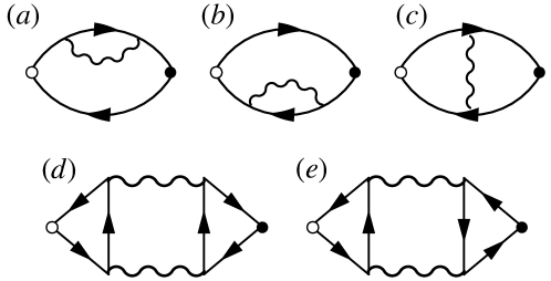
Figure 10: Interaction contributions to optical conductivity, to leading order in $1/N$. (a,b) are DOS diagrams, (c) is MT, and (d,e) are AL diagrams. The current vertices are labeled by circles. Open/solid circles represent the inflow/outflow of the external frequency $\Omega$.

In this section we show that at high external frequencies, our derivation of optical conductivity gives the same results as the standard perturbative calculation. From Kubo linear response theory, the dissipative part of optical conductivity is calculated from the imaginary part of the retarded current-current response function:

$$\sigma^{\prime}\left(\Omega\right)=\frac{1}{\Omega}\text{Im}\mathcal{G}_{JJ}\left(\Omega\right)$$ (90)

To leading order in $1/N$, there are three types of diagrams that contribute to $\sigma(\Omega)$, depicted in Figure 10(a-e). These are the so-called density of states (DOS), Maki-Thompson (MT), and Aslamazov-Larkin (AL) diagrams. We discuss these contributions in Matsubara frequency, and comment on the analytic continuation $i\Omega_{n}\rightarrow\Omega+i\delta$.

The DOS diagrams contribute two terms (a,b), related to each other by a change of $i\Omega_{n}\rightarrow-i\Omega_{n}$. They can be expressed as:

$$\begin{split}\mathcal{G}_{JJ}^{\text{DOS}}(i\Omega_{n})&=-\lambda^{2}T^{2}\sum_{\nu_{n}\omega_{n}}\sum_{\mathbf{k}\mathbf{q}}v_{\mathbf{k},x}^{2}f_{\mathbf{k,k+q}}^{2}D_{\mathbf{q},\nu_{n}}G_{\mathbf{k}+\mathbf{q},\omega_{n}+\nu_{n}}\\ &\times G_{\mathbf{k},\omega_{n}}^{2}\left(G_{\mathbf{k},\omega_{n}+\Omega_{n}}+G_{\mathbf{k},\omega_{n}-\Omega_{n}}\right).\end{split}$$ (91)

Here $G_{\mathbf{k},\omega_{n}}$ is short hand notation for the non-interacting fermionic Green’s function $G_{0}\left(\mathbf{k},i\omega_{n}\right)=\left(i\omega_{n}-\varepsilon_{\mathbf{k}}\right)^{-1}$. Making use of the identity $G_{\mathbf{k},\omega_{n}}G_{\mathbf{k},\omega_{n}+\Omega_{n}}=\frac{1}{i\Omega_{n}}\left(G_{\mathbf{k},\omega_{n}}-G_{\mathbf{k},\omega_{n}+\Omega_{n}}\right)$, it is straightforward to show:

$$\begin{split}\mathcal{G}_{JJ}^{\text{DOS}}(i\Omega_{n})&=\frac{\lambda^{2}T^{2}}{\Omega_{n}^{2}}\sum_{\nu_{n}\omega_{n}}\sum_{\mathbf{k}\mathbf{q}}v_{\mathbf{k},x}^{2}f_{\mathbf{k,k+q}}^{2}D_{\mathbf{q},\nu_{n}}G_{\mathbf{k}+\mathbf{q},\omega_{n}+\nu_{n}}\left(G_{\mathbf{k},\omega_{n}+\Omega_{n}}+G_{\mathbf{k},\omega_{n}-\Omega_{n}}\right)\\ &-\frac{\lambda^{2}T^{2}}{\Omega_{n}^{2}}\sum_{\nu_{n}\omega_{n}}\sum_{\mathbf{k}\mathbf{q}}v_{\mathbf{k},x}^{2}f_{\mathbf{k,k+q}}^{2}D_{\mathbf{q},\nu_{n}}G_{\mathbf{k}+\mathbf{q},\omega_{n}+\nu_{n}}G_{\mathbf{k},\omega_{n}}.\end{split}$$ (92)

The term on the second line does not contribute to $\sigma^{\prime}\left(\Omega\right)$, since following analytic continuation, it is the real part of the retarded response function. Focusing on the first term, by a suitable change of variables, the dependence on the external frequency can be shifted entirely into the nematic propagator:

$$\begin{split}\mathcal{G}_{JJ}^{\text{DOS}}(i\Omega_{n})&=-\frac{\lambda^{2}T}{\Omega_{n}^{2}}\sum_{\nu_{n}\omega_{n}}\sum_{\mathbf{k}\mathbf{q}}v_{\mathbf{k},x}^{2}\sum_{\zeta=\pm 1}f_{\mathbf{k,k+\zeta q}}^{2}D_{\mathbf{q},\nu_{n}+\Omega_{n}}R\left(\mathbf{k},\mathbf{k+\zeta q},i\zeta\nu_{n}\right)\end{split}$$ (93)

Here, as before $R\left(\mathbf{k},\mathbf{k+q},i\nu_{n}\right)\equiv-T\sum_{\omega_{n}}G_{\mathbf{k}+\mathbf{q},\omega_{n}+\nu_{n}}G_{\mathbf{k},\omega_{n}}$.

The MT term (c) can be expressed as:

$$\begin{split}\mathcal{G}_{JJ}^{\text{MT}}(i\Omega_{n})&=-\lambda^{2}T^{2}\sum_{\nu_{n}\omega_{n}}\sum_{\mathbf{k}\mathbf{k^{\prime}}\mathbf{q}}v_{\mathbf{k},x}v_{\mathbf{k^{\prime}},x}f_{\mathbf{k,k^{\prime}}}^{2}D_{\mathbf{q},\nu_{n}}\\ &\times G_{\mathbf{k},\omega_{n}}G_{\mathbf{k}+\mathbf{q},\omega_{n}+\Omega_{n}}G_{\mathbf{k}^{\prime},\omega_{n}+\nu_{n}+\Omega_{n}}G_{\mathbf{k}^{\prime},\omega_{n}+\nu_{n}}\end{split}$$ (94)

Following similar procedure as above, the MT contribution can be reduced to:

$$\mathcal{G}_{JJ}^{\text{MT}}(i\Omega_{n})=\frac{\lambda^{2}T}{\Omega_{n}^{2}}\sum_{\mathbf{kk^{\prime}}}v_{\mathbf{k},x}v_{\mathbf{k^{\prime}},x}\sum_{\mathbf{q}\nu_{n}}D_{\mathbf{q},\nu_{n}+\Omega_{n}}\sum_{\zeta=\pm 1}\delta_{\mathbf{k^{\prime}-k,\zeta q}}f_{\mathbf{k,k+\zeta q}}^{2}R\left(\mathbf{k},\mathbf{k+\zeta q},i\zeta\nu_{n}\right)$$ (95)

Eqs. (93) and (95) share a similar structure. The combination gives:

$$\begin{split}\mathcal{G}_{JJ}^{\text{DOS+MT}}\left(i\Omega_{n}\right)&=\frac{\lambda^{2}T}{\Omega_{n}^{2}}\sum_{\mathbf{kk^{\prime}}}v_{\mathbf{k},x}v_{\mathbf{k^{\prime}},x}\sum_{\mathbf{q}\nu_{n}}D_{\mathbf{q},\nu_{n}+\Omega_{n}}\\ &\times\sum_{\zeta=\pm 1}\left(\delta_{\mathbf{k^{\prime}-k,\zeta q}}-\delta_{\mathbf{kk^{\prime}}}\right)f_{\mathbf{k,k+\zeta q}}^{2}R\left(\mathbf{k},\mathbf{k+\zeta q},i\zeta\nu_{n}\right).\end{split}$$ (96)

The AL contribution (d,e) can be expressed as:

$$\begin{split}\mathcal{G}_{JJ}^{\text{AL}}(i\Omega_{n})&=\lambda^{4}T\sum_{\mathbf{q},\nu_{n}}D_{\mathbf{q},\nu_{n}}D_{\mathbf{q},\nu_{n}+\Omega_{n}}\\ &\times T\sum_{\mathbf{k}\omega_{n}}v_{\mathbf{k},x}G_{\mathbf{k},\omega_{n}-\Omega_{n}}G_{\mathbf{k},\omega_{n}}G_{\mathbf{k+q},\omega_{n}+\nu_{n}}\\ &\times T\sum_{\mathbf{k^{\prime}}\omega^{\prime}_{n}}v_{\mathbf{k^{\prime}},x}\left(G_{\mathbf{k^{\prime}},\omega^{\prime}_{n}-\Omega_{n}}G_{\mathbf{k^{\prime}},\omega^{\prime}_{n}}G_{\mathbf{k^{\prime}+q},\omega^{\prime}_{n}+\nu_{n}}+G_{\mathbf{k^{\prime}},\omega^{\prime}_{n}+\Omega_{n}}G_{\mathbf{k^{\prime}},\omega^{\prime}_{n}}G_{\mathbf{k^{\prime}-q},\omega^{\prime}_{n}-\nu_{n}}\right).\end{split}$$ (97)

Here the terms on the second and third lines represent the fermionic triangle. Similarly, it can be reduced to:

$$\begin{split}\mathcal{G}_{JJ}^{\text{AL}}(i\Omega_{n})&=-\frac{\lambda^{4}T}{\Omega_{n}^{2}}\sum_{\mathbf{k}\mathbf{k^{\prime}}}v_{\mathbf{k},x}v_{\mathbf{k^{\prime}},x}\sum_{\mathbf{q},\nu_{n}}D_{\mathbf{q},\nu_{n}}D_{\mathbf{q},\nu_{n}+\Omega_{n}}\\ &\times f_{\mathbf{k,k+q}}^{2}\left[R\left(\mathbf{k},\mathbf{k+q},i\nu_{n}\right)-R\left(\mathbf{k},\mathbf{k+q},i\nu_{n}+i\Omega_{n}\right)\right]\\ &\times\sum_{\zeta^{\prime}=\pm 1}f_{\mathbf{k^{\prime}},\mathbf{k^{\prime}+\zeta^{\prime}q}}^{2}\left[R\left(\mathbf{k^{\prime}},\mathbf{k^{\prime}}+\zeta^{\prime}\mathbf{q},i\zeta^{\prime}\nu_{n}\right)-R\left(\mathbf{k^{\prime}},\mathbf{k^{\prime}}+\zeta^{\prime}\mathbf{q},i\zeta^{\prime}\nu_{n}+i\zeta^{\prime}\Omega_{n}\right)\right].\end{split}$$ (98)

Comparing Eqs. (96) and (98) with our class I and class II diagrams for the memory matrix in Eqs (41), we see that DOS+MT correspond to class I diagram, and AL correspond to class II diagram. Specifically,

$$\begin{split}\mathcal{G}_{JJ}^{\text{DOS+MT}}\left(i\Omega_{n}\right)&=\frac{1}{\Omega_{n}^{2}}\sum_{\mathbf{kk^{\prime}}}v_{\mathbf{k},x}M_{\mathbf{kk^{\prime}}}^{(1)}\left(i\Omega_{n}\right)v_{\mathbf{k^{\prime}},x}\\ \mathcal{G}_{JJ}^{\text{AL}}\left(i\Omega_{n}\right)&=\frac{1}{\Omega_{n}^{2}}\sum_{\mathbf{kk^{\prime}}}v_{\mathbf{k},x}M_{\mathbf{kk^{\prime}}}^{(2)}\left(i\Omega_{n}\right)v_{\mathbf{k^{\prime}},x}\end{split}$$ (99)

We note, however, that $\sigma(i\Omega_{n})$ computed to lowest order in perturbation theory is equivalent to our memory matrix approach only at the high frequency limit. This is seen by expanding Eq. (42) to leading order in the memory matrix:

$$\begin{split}\sigma\left(i\Omega_{n}\right)&\approx\frac{1}{\Omega_{n}}\left(\chi_{J_{x}\mathbf{k}}\chi_{\mathbf{kk^{\prime}}}^{-1}\chi_{\mathbf{k}^{\prime}J_{x}}\right)-\frac{1}{\Omega_{n}^{2}}\chi_{J_{x}\mathbf{k}}\chi_{\mathbf{k}\mathbf{k}_{1}}^{-1}M_{\mathbf{k}_{1}\mathbf{k}_{2}}\chi_{\mathbf{k}_{1}\mathbf{k}^{\prime}}^{-1}\chi_{\mathbf{k}^{\prime}J_{x}}\\ &\approx\frac{1}{\Omega_{n}}\sum_{\mathbf{k}}v_{\mathbf{k},x}^{2}\frac{\partial n_{F}}{\partial\varepsilon_{\mathbf{k}}}-\frac{1}{\Omega_{n}^{2}}\sum_{\mathbf{kk^{\prime}}}v_{\mathbf{k},x}M_{\mathbf{kk^{\prime}}}(i\Omega_{n})v_{\mathbf{k}^{\prime},x}\end{split}$$ (100)

Repeated indices are summed over. In the second step we made use of $\mathbf{J}=\sum_{\mathbf{k}}\mathbf{v}_{\mathbf{k}}c_{\mathbf{k}}^{\dagger}c_{\mathbf{k}}$, and $\chi_{\mathbf{kk^{\prime}}}=\delta_{\mathbf{kk^{\prime}}}\left(-\partial_{\varepsilon_{\mathbf{k}}}n_{F}\right)$.

In the dc limit, $\sigma^{\prime}(\Omega\rightarrow 0)\propto M^{-1}$, which cannot be obtained perturbatively without resumming an infinite set of diagrams.

Appendix H Totally compensated metal

In a general band structure, the momentum and the current operators are not identical, and therefore electron-electron collisions can change the total current even if they conserve momentum. However, since the total electrical current has a finite overlap with the total momentum, meaning that the thermodynamic susceptibility $\chi_{\mathbf{JP}}\neq 0$, the dc resistivity is still zero as long as momentum is conserved, because then the current cannot relax to zero.

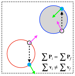
Figure 11: Sketch of a two-electron scattering process for compensated metal. Blue Fermi pockets are electron-like and red Fermi pocket is hole-like. The purple (green) arrows label the Fermi velocities in the initial (final) states. Such a process flips the direction of electrical current from upward to downward.

It is well-known, however, that this is not the case for a totally compensated metal, where the densities of electron and hole-like charge carriers are equal. This is because in a compensated metal, $\chi_{\mathbf{JP}}=0$. Below, we derive this result for completeness, first for non-interacting electrons and then a general interacting model. , As a result, in a compensated metal, the dc resistivity is non-zero even if momentum is perfectly conserved.

H.1 Non-interacting electrons

We consider a system with $i=1,\dots,l$ Fermi sheets. The current operator is given by $\mathbf{J}=-e\sum_{i\mathbf{k}}\mathbf{v}_{i\mathbf{k}}c_{i\mathbf{k}}^{\dagger}c_{i\mathbf{k}}$, where $\mathbf{v}_{ik}=\nabla_{\mathbf{k}}$$\varepsilon_{i\mathbf{k}}$, and $\varepsilon_{i\mathbf{k}}$ is the dispersion relation of the $i$th sheet, while the momentum operator is given by $\mathbf{P}=\sum_{i\mathbf{k}}\mathbf{k}c_{i\mathbf{k}}^{\dagger}c_{i\mathbf{k}}$. In the free electron limit, the thermodynamic susceptibility: $\chi_{\mathbf{JP}}=\int_{0}^{\beta}\mathrm{d}\tau\langle\mathbf{J}\left(\tau\right)\cdot\mathbf{P}(0)\rangle$ is given by:

$$\begin{split}\chi_{\mathbf{JP}}&=e\sum_{i\mathbf{k}}\mathbf{k}\cdot\mathbf{v}_{i\mathbf{k}}T\sum_{i\omega_{n}}G_{0i}^{2}\left(i\omega_{n},\varepsilon_{i\mathbf{k}}\right)\end{split}$$ (101)

Summing over Matsubara frequency gives $\frac{\partial n_{F}\left(\varepsilon_{i\mathbf{k}}\right)}{\partial\varepsilon_{i\mathbf{k}}}$. At temperatures much smaller than the Fermi energy of any of the Fermi sheets, we may approximate $\frac{\partial n_{F}\left(\varepsilon_{i\mathbf{k}}\right)}{\partial\varepsilon_{i\mathbf{k}}}\approx-\delta(\varepsilon_{\mathbf{k}})$. Then we have

$$\chi_{\mathbf{JP}} =-eL^{2}\sum_{i}\int\frac{d^{2}k}{\left(2\pi\right)^{2}}\mathbf{k}\cdot\mathbf{v}_{i\mathbf{k}}\delta(\varepsilon_{i\mathbf{k}})=-\frac{eL^{2}}{\left(2\pi\right)^{2}}\sum_{i}\oint_{FS}dk\mathbf{k}\cdot\hat{\mathbf{v}}_{i\mathbf{k}}.$$ (102)

Here, $L^{2}$ is the total area of the system. Note that $\oint_{FS}dk\mathbf{k}\cdot\hat{\mathbf{v}}_{i\mathbf{k}}$ is the area of the $i$th sheet in momentum space, with a positive sign if $\mathbf{v}_{i\mathbf{k}}$ is pointing outward (electron-like), and a negative sign if $\mathbf{v}_{i\mathbf{k}}$ is pointing inward (hole-like). Thus, by Eq. (102), $\chi_{\mathbf{JP}}$ is proportional to the total area of all the Fermi pockets, each weighted with a sign that corresponds to the type of carriers. In a compensated metal, this is zero by definition, and hence $\chi_{\mathbf{JP}}=0$.

H.2 Interacting compensated metal

We now derive this result in the presence of arbitrary interactions. We consider a general first-quantized Hamiltonian of the form

$$H=\sum_{j}\varepsilon_{j}\left(-i\nabla_{j}+q_{j}\mathbf{A}\right)+V(\{\mathbf{r}_{j}\})$$ (103)

where $\varepsilon_{j}(\mathbf{k})$ is the dispersion relation of the $j$th particle, and $V\left(\{\mathbf{r}_{j}\}\right)$ is an arbitrary interaction potential, assumed to be translationally invariant. Here, we have allowed for different types of carriers with different charges $q_{j}$. We would like to compute the overlap between the momentum and current operators:

$$\chi_{\mathbf{JP}}=\int_{0}^{\beta}\mathrm{d}\tau\left\langle\mathbf{P}(\tau)\cdot\left(\frac{\partial H}{\partial\mathbf{A}}\right)_{\mathbf{A}=0}\right\rangle$$ (104)

where $\mathbf{A}$ is spatially uniform. Since momentum is conserved, we can replace $\mathbf{P}(\tau)=\mathbf{P}(0)=\mathbf{P}.$ We write $\chi_{\mathbf{JP}}$ as

$$\begin{split}\chi_{\mathbf{JP}}&=\frac{1}{T}\frac{1}{Z}\text{Tr}\left[e^{-\beta H(\mathbf{A})}\left(\frac{\partial H}{\partial\mathbf{A}}\right)_{\mathbf{A}=0}\cdot\mathbf{P}\right]\\ &=-\frac{1}{T}\frac{1}{Z}\left\{\frac{\partial}{\partial\mathbf{A}}\cdot\text{Tr}\left[e^{-\beta H(\mathbf{A})}\mathbf{P}\right]\right\}_{\mathbf{A}=0}\\ &=-\frac{1}{T}\frac{1}{Z}\left\{\frac{\partial}{\partial\mathbf{A}}\cdot\text{Tr}\left[e^{-\beta H(\mathbf{A}=0)}(\mathbf{P}-\sum_{j}q_{j}\mathbf{A})\right]\right\}=\sum_{j}q_{j}\end{split}$$ (105)

where in the last line, we have performed a gauge transformation that shifts $-i\nabla_{j}\rightarrow-i\nabla_{j}-q_{j}\mathbf{A}$, and hence removes the $\mathbf{A}$ dependence from $H$ . In particular, if $\sum_{j}q_{j}=0$, i.e., in a totally compensated metal, then $\chi_{\mathbf{JP}}=0$. .

Appendix I Effect of the form factor and cold spots in compensated metal

In this Appendix, we derive the we derive the asymptotic behavior of $\rho(T)$ for a clean, compensated metal discussed in Sec. IV.3. As indicated in Fig. 7, the results depend qualitatively on the configuration of “cold spots” on the different Fermi sheets. Using a variational ansatz for the non-distribution function, we show that one can readily recover the different low-temperature exponents obtained numerically.

We use Eqs. (88,89) to write the dc resistivity as:

$$\rho(T)=\frac{\Phi^{T}M\Phi}{e^{2}(\Phi^{T}\chi V_{x})^{2}},$$ (106)

where, as before, we treat $\Phi$ as a vector in momentum, Fermi sheet, and flavor space. The computation of the resistivity can be treated as a minimization problem: $\Phi$ that satisfies Eq. (88) also minimizes the functional on the right hand side of Eq. (106) (Ziman, 1960). Hence, we can use Eq. (106) to bound the resistivity from above, by inserting a variational ansatz for $\Phi$. Crucially, for the ansatz we use below, the denominator of Eq. (106) will be essentially temperature independent. Hence, to find the temperature dependence of $\rho(T)$, we need to compute the numerator of (106) with our variational ansatz for $\Phi$.

From Eq. (82), we observe that

$$\begin{split}\rho\left(T\right)\propto&\lambda^{2}\sum_{ij;\mathbf{kk^{\prime}}}V_{\mathbf{k^{\prime}-k}}f_{i,\mathbf{k},\mathbf{k}^{\prime}}^{2}\delta\left(\varepsilon_{i\mathbf{k}}\right)\delta\left(\varepsilon_{i\mathbf{k^{\prime}}}\right)\\ &\times\left[\delta_{ij}\left(\Phi_{i\mathbf{k}}-\Phi_{i\mathbf{k^{\prime}}}\right)^{2}-\frac{\gamma_{j\mathbf{k^{\prime}-k}}}{\gamma_{\mathbf{k^{\prime}-k}}}\left(\Phi_{i\mathbf{k}}-\Phi_{i\mathbf{k}^{\prime}}\right)\left(\Phi_{j\mathbf{k}}-\Phi_{j\mathbf{k}^{\prime}}\right)\right]\end{split}$$ (107)

where $i,j$ are band labels, and we have replaced $h_{in\mathbf{k}}$ with $\Phi_{i\theta_{\mathbf{k}}}$, and replaced $d_{in,\mathbf{kk^{\prime}}}$ with $\Phi_{i\mathbf{k}}-\Phi_{i\mathbf{k}^{\prime}}$. By symmetry, $\Phi_{i\mathbf{k}}=-\Phi_{i,-\mathbf{k}}$. For concreteness, it is useful to consider a simple model with two circular Fermi pockets with opposite Fermi velocities; we will comment about the generalization to more generic situations below. In the two-pocket model, since the Fermi velocities of the two pockets are opposite, $\Phi_{1\mathbf{k}}=-\Phi_{2\mathbf{k}}$. Carrying out the summation over band as well as performing momentum integration along the direction perpendicular to the Fermi surface, we get:

$$\begin{split}\rho\left(T\right)\propto&\frac{k_{F}^{2}\lambda^{2}}{v_{F}^{2}}\oiint_{\theta\theta^{\prime}}\left(\Phi_{\theta}-\Phi_{\theta^{\prime}}\right)^{2}V_{\mathbf{k^{\prime}-k}}(T)\frac{f_{1\mathbf{k},\mathbf{k^{\prime}}}^{2}f_{2\mathbf{k},\mathbf{k^{\prime}}}^{2}}{f_{1\mathbf{k},\mathbf{k^{\prime}}}^{2}+f_{2\mathbf{k},\mathbf{k^{\prime}}}^{2}}\end{split}$$ (108)

Here, as before, $V_{\mathbf{q}}(T)=F(T/\omega_{\mathbf{q}})/\gamma_{\mathbf{q}}$, where $\omega_{\mathbf{q}}=r_{\mathbf{q}}/\gamma_{\mathbf{q}}$, $|\mathbf{k-k^{\prime}}|=2k_{F}\sin|\frac{\theta-\theta^{\prime}}{2}|$, and $F\left(x\right)=\frac{1}{x}\int_{-\infty}^{+\infty}\frac{\mathrm{d}u}{\pi}\frac{u^{2}}{1+u^{2}}\sinh^{-2}\left(\frac{u}{2x}\right)$. The asymptotic behavior of $F(x)$ is: for $x\ll 1$, $F\left(x\right)\propto x^{2}$; whereas for $x\gg 1$, $F\left(x\right)\propto x$.

Equation (108) forms the basis for carrying out scaling analysis. We analyze cases where either there are no cold spots on either pocket, a case with cold spots on both pockets, and a case where one pocket has cold spots and the other does not.

I.1 Absence of cold spots on either Fermi surface

In this case, we assume for simplicity that $f_{1}=f_{2}=1$. Since our the problem is rotationally invariant, the angular distribution function for an electric field in the $x$ direction is $\Phi_{\theta}=\cos\theta$ The dominant contribution to resistivity is due to small angle scattering. We define relative angle $\alpha\equiv|\theta-\theta^{\prime}|$, and the integrand of Eq. (108) for $\alpha\ll 1$:

$$\rho\left(T\right)\propto\int_{0}^{\theta_{0}}\mathrm{d}\alpha\alpha^{3}F\left(\frac{\theta_{T}}{\alpha{}^{3}}\right)$$ (109)

Here $\theta_{0}\sim 1$ is an upper cutoff. We defined $\theta_{T}\equiv T/\Omega_{L}$ to be a dimensionless temperature.

The integral is convergent both for $\alpha\rightarrow 0$ and $\alpha\rightarrow\infty$, due to the asymptotic behavior of the scaling function $F$ discussed above. Therefore, we can rescale $\tilde{\alpha}\equiv\alpha/\theta_{T}^{1/3}$, and extend the upper cutoff to infinity, resulting in $\rho(T)\propto\theta_{T}^{4/3}\sim T^{4/3}$.

I.2 Cold spots on both Fermi surfaces

As shown in Figs. 8(b) and (c), when cold spots are present, $\Phi_{\theta}$ deviates strongly from $\cos\theta$. In particular, $\Phi_{\theta}$ becomes nearly constant between each pair of cold spots. This motivates us to consider the following variational ansatz for $\Phi_{\theta}$:

$$\Phi_{\theta}\approx\begin{cases}1&\theta\in\left(-\frac{\pi}{4},\frac{\pi}{4}\right),\\ -1&\theta\in\left(\frac{3\pi}{4},\frac{5\pi}{4}\right),\\ 0&\text{elsewhere}.\end{cases}$$ (110)

The contribution to Eq. (108) then comes purely from scattering processes relating different angular regions. Let us consider the vicinity of the cold spot at $\theta=\frac{\pi}{4}$. Near the cold spot, we get:

$$\rho\left(T\right)\propto\int_{0}^{\theta_{0}}\alpha\mathrm{d}\alpha\int_{0}^{\alpha}\mathrm{d}\varphi F\left(\frac{\theta_{T}\varphi^{2}}{\alpha^{3}}\right).$$ (111)

Here we defined $\varphi\equiv\left|\frac{\theta+\theta^{\prime}}{2}-\frac{\pi}{4}\right|$ and $\alpha\equiv|\theta-\theta^{\prime}|$. Compared to the case when cold spots are absent, the scaling properties are not only determined the relative angle $\alpha$ between the momentum states, but also the average angle $\varphi$ with respect to the location of the cold spot. To extract the scaling of the resisitivity with $T$, we split the integration domain into two regions:

1. $\theta_{T}<\alpha<\theta_{0}$: Since in this regime the argument of $F$ in the integrand is smaller than unity, we estimate the integral by replacing $F(x)$ by its small $x$ behavior: $F\sim x^{2}$. The contribution of this regime is then estimated as $\Delta\rho_{2}\sim\int_{0}^{\theta_{0}}\alpha\mathrm{d}\alpha\int_{0}^{\alpha}\mathrm{d}\varphi\left(\theta_{T}\varphi^{2}\alpha^{-3}\right)^{2}\sim\theta_{0}\theta_{T}^{2}$. Notice that this contribution arises from large angle scattering, and hence it is proportional to $\theta_{0}$. This justifies considering $\alpha$ as much larger than $\theta_{T}$.

2. $0<\alpha<\theta_{T}$: in this regime, we perform a change of variables as follows: $\alpha=\tilde{\alpha}/\theta_{T}$, $\varphi=\tilde{\varphi}/\theta_{T}$. The integral becomes $\Delta\rho_{2}\sim\theta_{T}^{3}\int_{0}^{1}\tilde{\alpha}\mathrm{d}\tilde{\alpha}\int_{0}^{\tilde{\alpha}}\mathrm{d}\tilde{\varphi}F\left(\tilde{\varphi}^{2}\tilde{\alpha}^{-3}\right)\sim\theta_{T}^{3}$. This contribution is subleading compared to $\Delta\rho_{1}$.

As a result, at low temperatures and when the nematic cold spots are present on both Fermi surfaces, $\rho(T)\propto T^{2}$ due to scattering off non-critical nematic fluctuations carrying large momenta.

I.3 Cold spots on part of the Fermi surfaces

We consider a system with cold spots on the first Fermi sheet but not on the second. In this case, we may replace $f_{2}=1.$ For $\mathbf{q}$ pointing near the direction of the cold spots, the Landau damping coefficient $\gamma_{\mathbf{q}}\approx\gamma_{2,\mathbf{q}}$, and we can neglect its angular dependence. We use the same variational ansatz as for case B [Eq. (110)]. Again expanding near $\theta\left(\theta^{\prime}\right)\approx\frac{\pi}{4}$, we find that

$$\rho(T)\propto\int_{0}^{\theta_{0}}\alpha\mathrm{d}\alpha\int_{0}^{\alpha}\mathrm{d}\varphi\varphi^{2}F\left(\frac{\theta_{T}}{\alpha^{3}}\right),$$ (112)

where the factor of $\varphi^{2}$ comes from $f_{1}$ in Eq. (108). As a result, $\rho(T)\sim\int_{0}^{\theta_{0}}\alpha\mathrm{d}\alpha\int_{0}^{\alpha}\mathrm{d}\varphi\varphi^{2}F\left(\frac{\theta_{T}}{\alpha^{3}}\right)\sim\theta_{T}^{5/3}$. In this case, the resistivity comes mostly from small-angle scattering in the vicinity of $\theta\left(\theta^{\prime}\right)\approx\frac{\pi}{4}$.

We comment on the generalization for the more generic case with more two pockets, and where the shape of the pockets is non-circular. In this case, we use a variational ansatz where $\Phi$ is of the form (110) on the pockets with cold spots, and zero on the pockets where cold spots are absent. Evalutaing Eq. (107) along the same lines as above gives again $\rho(T)\sim\theta_{T}^{5/3}\sim T^{5/3}$, as in our two-pocket toy model. It is worth noting that this is an upper bound on the resistivity, and it only provides a lower bound on the resistivity exponent at low temperature. The numerical results for the two-pocket case [Fig. 6(b)] suggest the exponent is indeed $5/3$.

Appendix J Numerical construction of the memory matrix

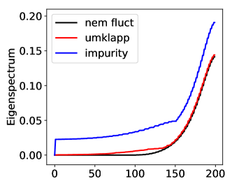
Figure 12: Eigenspectrum of the memory matrix $M_{\theta,\theta^{\prime}}$ for a single Fermi surface when only quantum critical scattering is considered (black), when umklapp scattering is included (red), and when quenched random impurity is included (blue). In this calculation, we used the dispersion $\varepsilon_{\mathbf{k}}=-2t\left(\cos k_{x}+\cos k_{y}\right)-4t^{\prime}\cos k_{x}\cos k_{y}-\mu$ , with $t=1$, $t^{\prime}=-0.3$ and $\mu=-1$. The nematic coupling strength is $\lambda^{2}\approx 2.62\varepsilon_{F}$, and impurity strength is $g_{\text{imp}}\approx 0.02\varepsilon_{F}$. The spectrum is obtained at temperature $T\approx 0.04\varepsilon_{F}$. We used 200 points to uniformly discretize the Fermi surface.

In this section we provide details on the construction of the memory matrix in the dc limit, as well as further numerical results.

We always work in the limit that temperature is much smaller than the Fermi energy. This allows us to project all scattering processes onto the Fermi surface, and perform integration over the momentum direction perpendicular to the Fermi surface. In practice, we use expressions in Eqs. (54) and (67) to construct the radially-integrated memory matrix. For a generic multi-Fermi surface system,

$$M_{i\theta,j\theta^{\prime}}=\int\frac{\mathrm{d}k_{i,\perp}\mathrm{d}k_{j,\perp}^{\prime}}{\left(2\pi\right)^{4}}M_{i\mathbf{k},j\mathbf{k^{\prime}}}$$ (113)

and the dc conductivity is calculated as

$$\sigma=\frac{e^{2}}{\hbar}\int\frac{\mathrm{d}k_{i,\parallel}\mathrm{d}k^{\prime}_{j,\parallel}}{\left(2\pi\right)^{4}}v_{i\mathbf{k}}M_{i\mathbf{\theta},j\theta^{\prime}}^{-1}v_{j\mathbf{k}^{\prime}}$$ (114)

Here $v_{i\mathbf{k}}$ is the Fermi velocity of the $i$th band, and $\theta$ is the angle of $\mathbf{k}$ with respect to the $x$ direction. $\mathrm{d}k_{i,\parallel}=k_{iF}(\theta)\mathrm{d}\theta$.

The off-diagonal elements ($\mathbf{\theta\neq\theta^{\prime}}$) of the memory matrix are constructed from Eqs. (77) by solving for the condition that all participating momentum states are on the Fermi surface. For class I diagram, the following expression is used:

$$\begin{split}M_{i\theta,j\theta^{\prime}}^{(1)}&=-\delta_{ij}\frac{\lambda^{2}}{8\pi^{3}}\frac{f_{i,\mathbf{k},\mathbf{k^{\prime}}}^{2}V_{\mathbf{k^{\prime}-k}}}{v_{i\mathbf{k}}v_{i\mathbf{k}^{\prime}}}\end{split}$$ (115)

where on the right hand side both $\mathbf{k}$ and $\mathbf{k^{\prime}}$ are taken to be on the Fermi surface. Class II diagrams are constructed using:

$$\begin{split}M_{i\theta,j\theta^{\prime}}^{(2,+)}&=-\frac{\lambda^{4}}{32\pi^{4}}\sum_{\mathbf{q}=\mathbf{q}_{c}}\frac{V_{\mathbf{q}}}{\gamma_{\mathbf{q}}}f_{i,\mathbf{k},\mathbf{k}+\mathbf{q}}^{2}f_{j,\mathbf{k}^{\prime},\mathbf{k}^{\prime}+\mathbf{q}}^{2}\frac{1}{v_{i\mathbf{k}}v_{j\mathbf{k^{\prime}}}}\frac{1}{\left|\mathbf{v}_{i\mathbf{k+q}}\times\mathbf{v}_{j\mathbf{k^{\prime}+q}}\right|},\\ M_{i\theta,j\theta^{\prime}}^{(2,-)}&=\frac{\lambda^{4}}{32\pi^{4}}\sum_{\mathbf{q}=\mathbf{q}_{c}}\frac{V_{\mathbf{q}}}{\gamma_{\mathbf{q}}}f_{i,\mathbf{k},\mathbf{k}+\mathbf{q}}^{2}f_{j,\mathbf{k}^{\prime},\mathbf{k}^{\prime}-\mathbf{q}}^{2}\frac{1}{v_{i\mathbf{k}}v_{j\mathbf{k^{\prime}}}}\frac{1}{\left|\mathbf{v}_{i\mathbf{k+q}}\times\mathbf{v}_{j\mathbf{k^{\prime}-q}}\right|}\end{split}$$ (116)

Here all four momentum states $\mathbf{k},\mathbf{k^{\prime}},\mathbf{k+q}_{c}$ and $\mathbf{k^{\prime}\pm q}_{c}$ are on the Fermi surface. Note that the head-on collisions (namely when $\mathbf{k^{\prime}}=-\mathbf{k}$) need to be treated differently, as in this case, there is a one-dimensional manifold of $\mathbf{q}_{c}$ satisfying the momentum-energy conservation constraints. Specifically, we incoporate these processes using the following expression:

$$M_{i\theta,i\left(\theta+\pi\right)}^{(2)}=\int\mathrm{d}k^{\prime}_{i,\parallel}M_{i\theta,i\theta^{\prime}}^{(2,+)}$$

Finally, the diagonal elements of the memory matrix are constructed from number conservation, namely,

$$M_{i\theta,i\theta}=\sum_{j}\int\mathrm{d}k^{\prime}_{j,\parallel}M_{i\theta,j\theta^{\prime}}$$

In numerical calculations, we discretize the angle along the Fermi surface. The number of points is usually taken to be 500. However, to extract proper scaling behavior at the lowest temperatures, we checked the convergence of the results for up to 2000 points.

In Figure 12, we illustrate the properties of the eigenvalues of the memory matrix for a single Fermi surface. We present the case when only quantum critical scattering is present, as well as when current-relaxing mechanisms such as impurity and umklapp processes are incorporated.

In the absence of impurity or umklapp, there is a large number of zero modes, corresponding to the conservation of total electron number as well as the conservation of all odd-parity modes. This is expected since we are projecting scattering processes onto the Fermi surface. When either impurity or umklapp scattering is added, all odd-parity modes (including momentum) are lifted from zero, and only total number is conserved. However, the way these zero modes get lifted is different depending on the mechanism. In the case of impurity scattering, all odd-parity modes gain a finite decay rate $\sim g_{\text{imp}}^{2}\nu_{F}$. However when umklapp scattering is dominant, the odd-parity modes are smoothly lifted from $0$, and form a continuous spectrum.

References

- Scalapino (2012) D. J. Scalapino, “A common thread: The pairing interaction for unconventional superconductors,” Rev. Mod. Phys. 84, 1383–1417 (2012).
- Dell’Anna and Metzner (2007) Luca Dell’Anna and Walter Metzner, “Electrical resistivity near pomeranchuk instability in two dimensions,” Phys. Rev. Lett. 98, 136402 (2007).
- Hartnoll et al. (2014) Sean A. Hartnoll, Raghu Mahajan, Matthias Punk, and Subir Sachdev, “Transport near the ising-nematic quantum critical point of metals in two dimensions,” Physical Review B 89 (2014).
- Lederer et al. (2017) Samuel Lederer, Yoni Schattner, Erez Berg, and Steven A Kivelson, “Superconductivity and non-fermi liquid behavior near a nematic quantum critical point,” Proceedings of the National Academy of Sciences , 201620651 (2017).
- Maslov et al. (2011) Dmitrii L. Maslov, Vladimir I. Yudson, and Andrey V. Chubukov, “Resistivity of a non-galilean–invariant fermi liquid near pomeranchuk quantum criticality,” Phys. Rev. Lett. 106, 106403 (2011).
- Fradkin et al. (2010) Eduardo Fradkin, Steven A. Kivelson, Michael J. Lawler, James P. Eisenstein, and Andrew P. Mackenzie, “Nematic fermi fluids in condensed matter physics,” Annual Review of Condensed Matter Physics 1, 153–178 (2010).
- Chu et al. (2010) Jiun-Haw Chu, James G. Analytis, Kristiaan De Greve, Peter L. McMahon, Zahirul Islam, Yoshihisa Yamamoto, and Ian R. Fisher, “In-plane resistivity anisotropy in an underdoped iron arsenide superconductor,” Science 329, 824–826 (2010).
- Fernandes et al. (2014) R. M. Fernandes, A. V. Chubukov, and J. Schmalian, “What drives nematic order in iron-based superconductors?” Nature Physics 10, 97–104 (2014).
- Hosoi et al. (2016) Suguru Hosoi, Kohei Matsuura, Kousuke Ishida, Hao Wang, Yuta Mizukami, Tatsuya Watashige, Shigeru Kasahara, Yuji Matsuda, and Takasada Shibauchi, “Nematic quantum critical point without magnetism in fese1- xsx superconductors,” Proceedings of the National Academy of Sciences 113, 8139–8143 (2016).
- Coldea and Watson (2018) Amalia I. Coldea and Matthew D. Watson, “The key ingredients of the electronic structure of fese,” Annual Review of Condensed Matter Physics 9, 125–146 (2018).
- Kohsaka et al. (2007) Y. Kohsaka, C. Taylor, K. Fujita, A. Schmidt, C. Lupien, T. Hanaguri, M. Azuma, M. Takano, H. Eisaki, H. Takagi, S. Uchida, and J.C. Davis, “An intrinsic bond-centered electronic glass with unidirectional domains in underdoped cuprates,” Science 315, 1380–1385 (2007).
- Daou et al. (2010) R. Daou, J. Chang, David LeBoeuf, Olivier Cyr-Choinière, Francis Laliberté, Nicolas Doiron-Leyraud, B. J. Ramshaw, Ruixing Liang, D. A. Bonn, W. N. Hardy, and et al., “Broken rotational symmetry in the pseudogap phase of a high-tc superconductor,” Nature 463, 519–522 (2010).
- Kasahara et al. (2010) S. Kasahara, T. Shibauchi, K. Hashimoto, K. Ikada, S. Tonegawa, R. Okazaki, H. Shishido, H. Ikeda, H. Takeya, K. Hirata, T. Terashima, and Y. Matsuda, “Evolution from non-fermi- to fermi-liquid transport via isovalent doping in superconductors,” Phys. Rev. B 81, 184519 (2010).
- Reiss et al. (2017) P. Reiss, M. D. Watson, T. K. Kim, A. A. Haghighirad, D. N. Woodruff, M. Bruma, S. J. Clarke, and A. I. Coldea, “Suppression of electronic correlations by chemical pressure from fese to fes,” Phys. Rev. B 96, 121103 (2017).
- Urata et al. (2016) Takahiro Urata, Yoichi Tanabe, Khuong Kim Huynh, Hidetoshi Oguro, Kazuo Watanabe, and Katsumi Tanigaki, “Non-fermi liquid behavior of electrical resistivity close to the nematic critical point in Fe1-xCoxSe and FeSe1-ySy,” arXiv:1608.01044 (2016).
- (16) P. Reiss, D. Graf, A. A. Haghighirad, W. Knafo, L. Drigo, M. Bristow, A. J. Schofield, and A. I. Coldea, “Quenched nematic criticality separating two superconducting domes in an iron-based superconductor under pressure,” To appear.
- Varma et al. (1989) CM Varma, P Be Littlewood, S Schmitt-Rink, E Abrahams, and AE Ruckenstein, “Phenomenology of the normal state of cu-o high-temperature superconductors,” Phys. Rev. Lett. 63, 1996 (1989).
- Kim et al. (1995) Yong Baek Kim, Patrick A. Lee, and Xiao-Gang Wen, “Quantum boltzmann equation of composite fermions interacting with a gauge field,” Phys. Rev. B 52, 17275–17292 (1995).
- Hlubina and Rice (1995) R. Hlubina and T. M. Rice, “Resistivity as a function of temperature for models with hot spots on the fermi surface,” Phys. Rev. B 51, 9253–9260 (1995).
- Rosch (1999) A. Rosch, “Interplay of disorder and spin fluctuations in the resistivity near a quantum critical point,” Phys. Rev. Lett. 82, 4280–4283 (1999).
- Syzranov and Schmalian (2012) S. V. Syzranov and J. Schmalian, “Conductivity close to antiferromagnetic criticality,” Phys. Rev. Lett. 109, 156403 (2012).
- Paul et al. (2013) I. Paul, C. Pépin, and M. R. Norman, “Equivalence of single-particle and transport lifetimes from hybridization fluctuations,” Phys. Rev. Lett. 110, 066402 (2013).
- Patel and Sachdev (2014) Aavishkar A. Patel and Subir Sachdev, “dc resistivity at the onset of spin density wave order in two-dimensional metals,” Phys. Rev. B 90, 165146 (2014).
- Chubukov et al. (2014) Andrey V. Chubukov, Dmitrii L. Maslov, and Vladimir I. Yudson, “Optical conductivity of a two-dimensional metal at the onset of spin-density-wave order,” Phys. Rev. B 89, 155126 (2014).
- Chubukov and Maslov (2017) Andrey V. Chubukov and Dmitrii L. Maslov, “Optical conductivity of a two-dimensional metal near a quantum critical point: The status of the extended drude formula,” Phys. Rev. B 96, 205136 (2017).
- Metzner et al. (2003) W. Metzner, D. Rohe, and S. Andergassen, “Soft fermi surfaces and breakdown of fermi-liquid behavior,” Phys. Rev. Lett. 91, 066402 (2003).
- Oganesyan et al. (2001) Vadim Oganesyan, Steven A. Kivelson, and Eduardo Fradkin, “Quantum Theory of a Nematic Fermi Fluid,” Phys. Rev. B 64, 195109 (2001).
- Rech et al. (2006) Jérôme Rech, Catherine Pépin, and Andrey V. Chubukov, “Quantum critical behavior in itinerant electron systems: Eliashberg theory and instability of a ferromagnetic quantum critical point,” Phys. Rev. B 74, 195126 (2006).
- Lawler et al. (2006) Michael J. Lawler, Daniel G. Barci, Victoria Fernández, Eduardo Fradkin, and Luis Oxman, “Nonperturbative behavior of the quantum phase transition to a nematic fermi fluid,” Phys. Rev. B 73, 085101 (2006).
- Löhneysen et al. (2007) Hilbert v. Löhneysen, Achim Rosch, Matthias Vojta, and Peter Wölfle, “Fermi-liquid instabilities at magnetic quantum phase transitions,” Rev. Mod. Phys. 79, 1015–1075 (2007).
- Lee (2009) Sung-Sik Lee, “Low-energy effective theory of fermi surface coupled with u(1) gauge field in dimensions,” Phys. Rev. B 80, 165102 (2009).
- Zacharias et al. (2009) Mario Zacharias, Peter Wölfle, and Markus Garst, “Multiscale quantum criticality: Pomeranchuk instability in isotropic metals,” Phys. Rev. B 80, 165116 (2009).
- Mross et al. (2010) David F. Mross, John McGreevy, Hong Liu, and T. Senthil, “Controlled expansion for certain non-fermi-liquid metals,” Phys. Rev. B 82, 045121 (2010).
- Metlitski and Sachdev (2010) Max A. Metlitski and Subir Sachdev, “Quantum phase transitions of metals in two spatial dimensions. i. ising-nematic order,” Phys. Rev. B 82, 075127 (2010).
- Dalidovich and Lee (2013) Denis Dalidovich and Sung-Sik Lee, “Perturbative non-fermi liquids from dimensional regularization,” Phys. Rev. B 88, 245106 (2013).
- Holder and Metzner (2015) Tobias Holder and Walter Metzner, “Anomalous dynamical scaling from nematic and u(1) gauge field fluctuations in two-dimensional metals,” Phys. Rev. B 92, 041112 (2015).
- Klein et al. (2018a) Avraham Klein, Samuel Lederer, Debanjan Chowdhury, Erez Berg, and Andrey Chubukov, “Dynamical susceptibility of a near-critical nonconserved order parameter and quadrupole raman response in fe-based superconductors,” Phys. Rev. B 98, 041101 (2018a).
- Klein et al. (2018b) Avraham Klein, Samuel Lederer, Debanjan Chowdhury, Erez Berg, and Andrey Chubukov, “Dynamical susceptibility near a long-wavelength critical point with a nonconserved order parameter,” Phys. Rev. B 97, 155115 (2018b).
- Hertz (1976) John A. Hertz, “Quantum critical phenomena,” Phys. Rev. B 14, 1165–1184 (1976).
- Millis (1993) A. J. Millis, “Effect of a nonzero temperature on quantum critical points in itinerant fermion systems,” Phys. Rev. B 48, 7183–7196 (1993).
- Moriya (1985) Tôru Moriya, “Spin fluctuations in itinerant electron magnetism,” Springer Series in Solid-State Sciences (1985).
- Schattner et al. (2016) Yoni Schattner, Samuel Lederer, Steven A. Kivelson, and Erez Berg, “Ising nematic quantum critical point in a metal: A monte carlo study,” Phys. Rev. X 6, 031028 (2016).
- Berg et al. (2019) Erez Berg, Samuel Lederer, Yoni Schattner, and Simon Trebst, “Monte carlo studies of quantum critical metals,” Annual Review of Condensed Matter Physics 10 (2019).
- Ledwith et al. (2017) Patrick J Ledwith, Haoyu Guo, Andrey V Shytov, and Leonid Levitov, “Tomographic dynamics and scale-dependent viscosity in two-dimensional electron systems,” arXiv:1708.02376 (2017).
- Note (1) This is the case, for instance, if the order parameter has symmetry and some of the Fermi pockets are centered away from the high symmetry points , in the Brillouin zone, as in many of the iron-based superconductors.
- Note (2) This regime is accessible, within our model, in the limit where the number of fermion flavors is large.
- Note (3) The expression for the bare propagator has lattice effects included, i.e., , where is any reciprocal lattice wavevector. Later on when we study transport properties of a compensated metal, we will instead use the continuous expression: .
- Kadanoff and Martin (1963) Leo P Kadanoff and Paul C Martin, “Hydrodynamic equations and correlation functions,” Annals of Physics 24, 419 – 469 (1963).
- Forster (March 8, 2018) D. Forster, Hydrodynamic Fluctuations, Broken Symmetry, And Correlation Functions (CRC Press; 1 edition, March 8, 2018).
- Götze and Wölfle (1972) W. Götze and P. Wölfle, “Homogeneous dynamical conductivity of simple metals,” Phys. Rev. B 6, 1226–1238 (1972).
- Rosch and Andrei (2000) A. Rosch and N. Andrei, “Conductivity of a clean one-dimensional wire,” Phys. Rev. Lett. 85, 1092–1095 (2000).
- Shimshoni et al. (2003) E. Shimshoni, N. Andrei, and A. Rosch, “Thermal conductivity of spin- chains,” Phys. Rev. B 68, 104401 (2003).
- Jung and Rosch (2007) Peter Jung and Achim Rosch, “Lower bounds for the conductivities of correlated quantum systems,” Phys. Rev. B 75, 245104 (2007).
- Mahajan et al. (2013) Raghu Mahajan, Maissam Barkeshli, and Sean A. Hartnoll, “Non-fermi liquids and the wiedemann-franz law,” Phys. Rev. B 88, 125107 (2013).
- Lucas and Sachdev (2015) Andrew Lucas and Subir Sachdev, “Memory matrix theory of magnetotransport in strange metals,” Phys. Rev. B 91, 195122 (2015).
- Hartnoll et al. (2018) Sean A. Hartnoll, Andrew Lucas, and Subir Sachdev, Holographic Quantum Matter (MIT Press, 2018).
- Note (4) Since the interaction is momentum dependent, it also contributes a term to the current operator. However, this term is subleading in and in , and will be neglected.
- Note (5) The precise meaning of these operators being nearly conserved is elaborated on in Appendix A.1.
- Note (6) To do this, one introduces a field which is the conjugate momentum of . The Hamilontian then contains a term , where the “mass” is taken to at the end of the calculation.
- Kadanoff and Baym (1962) Leo P Kadanoff and Gordon Baym, Quantum statistical mechanics (W A Benjamin, 1962).
- Rammer and Smith (1986) J. Rammer and H. Smith, “Quantum field-theoretical methods in transport theory of metals,” Rev. Mod. Phys. 58, 323–359 (1986).
- Kamenev (2011) Alex Kamenev, Field Theory of Non-equilibrium Systems (Cambridge University Press, 2011).
- Note (7) Complications due to non-convex Fermi surfaces Maslov et al. (2011) can easily be incorporated within the same formalism, but will not be considered here.
- Gurzhi et al. (1995) R. N. Gurzhi, A. N. Kalinenko, and A. I. Kopeliovich, “Electron-electron momentum relaxation in a two-dimensional electron gas,” Phys. Rev. B 52, 4744–4747 (1995).
- Note (8) The cross term is negligible as long as the disorder potential does not couple linearly to the nematic order parameter. Such coupling is generated at higher order in disorder, but we assume it to be small. Transport in the presence of “random field” disorder that couples linearly to the nematic order parameter was considererd in Ref. Hartnoll et al. (2014). At sufficiently low temperature, this type of disorder is likely to qualitatively modify the properties of the quantum critical point, as well as its transport properties.
- Baber and Mott (1937) W. G. Baber and N. F. Mott, “The contribution to the electrical resistance of metals from collisions between electrons,” Proc. Roy. Soc. London 158, 383 (1937) 158, 383–396 (1937).
- Böhmer and Meingast (2016) Anna E. Böhmer and Christoph Meingast, “Electronic nematic susceptibility of iron-based superconductors,” Comptes Rendus Physique 17, 90 – 112 (2016).
- Zacharias et al. (2015) Mario Zacharias, Indranil Paul, and Markus Garst, “Quantum critical elasticity,” Phys. Rev. Lett. 115, 025703 (2015).
- Karahasanovic and Schmalian (2016) U. Karahasanovic and J. Schmalian, “Elastic coupling and spin-driven nematicity in iron-based superconductors,” Phys. Rev. B 93, 064520 (2016).
- Paul and Garst (2017) I. Paul and M. Garst, “Lattice effects on nematic quantum criticality in metals,” Phys. Rev. Lett. 118, 227601 (2017).
- Note (9) To appreciate the significance of this point, it is useful to note that in contrast, the matrix element between the operator and is . This is because does not commute with the kinetic energy, and hence is not suppressed by a factor of .
- Note (10) There is a subtlety at this step: if we use periodic boundary conditions, then a gauge transformation can only shift the vector potential by integer multiples of , where is the system’s spatial dimention. This can be remedied by approximating, e.g., with , and taking the limit .
- Ziman (1960) J. M. Ziman, Electrons and phonons: the theory of transport phenomena in solids (Oxford Univ. Press, London and New York, 1960).