Neutrino Masses and Mixing: A Little History for a Lot of Fun

Abstract

In this talk I present my personal summary of the progress on the determination of the masses of the neutrinos and of the leptonic flavour mixing from the combined analysis of the experimental results.

1 Prologue: Perspective from Fall 2018

I start this talk on the piece of history that the organizers asked me to cover by describing the end of the history so far, ie the present, September 2018.

We stand here 50 years after the first results from the Chlorine experiment which measured a flux of $\nu_{e}$ from the Sun which came out to be a bit too small compared to the expectations [1] launching the neutrino flavour oscillation adventure. Since then we have been gathering data from a large number of neutrino experiments performed with a variety of neutrino sources, and covering a wide range of neutrino energies. The progress (which sometimes came with the associated confusion) on the experimental front has been covered in the talks of (in order of appearance) T. Kirsten [1], P. Lipari [2], J. Learned [3], P. Vogel [4], K. Kleinkecht [5], G. Feldman [6], T. Kajita [7], A. McDonald [8], and T. Lasierre [9]. From their results we have established with high or at least good precision that:

$\bullet$ Atmospheric $\nu_{\mu}$ and $\bar{\nu}_{\mu}$ disappear most likely converting to $\nu_{\tau}$ and $\bar{\nu}_{\tau}$. The results show an energy and distance dependence perfectly described by mass-induced oscillations.

$\bullet$ Accelerator $\nu_{\mu}$ and $\bar{\nu}_{\mu}$ disappear over distances of $\sim$ 200 to 700 Km. The energy spectrum of the results show a clear oscillatory behaviour also in accordance with mass-induced oscillations.

$\bullet$ Solar $\nu_{e}$ convert to $\nu_{\mu}$ and/or $\nu_{\tau}$. The observed energy dependence of the effect is well described by neutrino conversion in the Sun matter according to the MSW effect [10].

$\bullet$ Reactor $\bar{\nu}_{e}$ disappear over distances of $\sim$ 200 Km and $\sim$ 1.5 km with different probabilities. The observed energy spectra show two different mass-induced oscillation wavelengths: at short distances in agreement with the one observed in accelerator $\nu_{\mu}$ disappearance, and a long distance compatible with the required parameters for MSW conversion in the Sun.

$\bullet$ Accelerator $\nu_{\mu}$ and $\bar{\nu}_{\mu}$ appear as $\nu_{e}$ and $\bar{\nu}_{e}$ at distances $\sim$ 200 to 700 Km.

All these results imply that neutrinos are massive and there is physics beyond the Standard Model (SM). The logic behind this statement is that a fermion mass term couples right-handed and left-handed fermions. But the SM, a gauge theory based on the gauge symmetry $SU(3)_{\rm C}\times SU(2)_{\rm L}\times U(1)_{\rm Y}$ – spontaneously broken to $SU(3)_{\rm C}\times U(1)_{\rm EM}$ by the the vacuum expectation value of a Higgs doublet field $\phi$ –, contains three fermion generations which reside in the chiral representations of the gauge group required to describe their interactions. As such, right-handed fields are included for charged fermions since they are needed to build the electromagnetic and strong currents. But no right-handed neutrino is included in the model because neutrinos are neutral and colourless and therefore the right-handed neutrinos are singlets of the SM group (hence unrequired). This also implies that total lepton number ($L$) is a global a symmetry of the model. A symmetry which is non-anomalous. So within the framework of the SM no mass term can be built for the neutrinos at any order in perturbation theory neither from non-perturbative effects. This is, SM predicts that neutrinos are strictly massless. Consequently, there is neither mixing nor CP violation in the leptonic sector. Clearly this is in contradiction with the neutrino data as summarized above.

The fundamental question opened by those results is that of the underlying beyond the standard model theory for neutrino masses and P. Ramond [11] has discussed such theoretical implications. But as for the description of the data we can live with an effective model consisting of the Standard Model minimally extended to include neutrino masses. This minimal extension is what I call The New Minimal Standard Model (NMSM).

The two minimal extensions to give neutrino mass and explain the data are:

$\bullet$ Introduce $\nu_{R}$ and impose $L$ conservation so after spontaneuous electroweak symmetry breaking

$${\cal L}_{D}={\cal L}_{SM}-M_{\nu}\bar{\nu}_{L}\nu_{R}+h.c.$$ (1)

In this case mass eigenstate neutrinos are Dirac fermions, ie $\nu^{C}\neq\nu$.

$\bullet$ Construct a mass term only with the SM left-handed neutrinos by allowing $L$ violation

$${\cal L}_{M}={\cal L}_{SM}-\frac{1}{2}M_{\nu}\bar{\nu}_{L}\nu^{c}_{L}+h.c.$$ (2)

In this case the mass eigenstates are Majorana fermions, $\nu^{C}=\nu$. Furthermore the Majorana mass term above also breaks the electroweak gauge invariance. In this respect ${\cal L}_{M}$ can only be understood as a low energy limit of a complete theory while ${\cal L}_{D}$ is formally self-consistent.

Either way, in the NMSM flavour is mixed in the CC interactions of the leptons, and a leptonic mixing matrix appears analogous to the CKM matrix for the quarks. However the discussion of leptonic mixing is complicated by two factors. First the number massive neutrinos is unknown, since there are no constraints on the number of right-handed, SM-singlet, neutrinos. Second, since neutrinos carry neither color nor electromagnetic charge, they could be Majorana fermions. As a consequence the number of new parameters in the model depends on the number of massive neutrino states and on whether they are Dirac or Majorana particles.

In general, if we denote the neutrino mass eigenstates by $\nu_{i}$, $i=1,2,\ldots,n$, and the charged lepton mass eigenstates by $l_{i}=(e,\mu,\tau)$, in the mass basis, leptonic CC interactions are given by

$$-{\cal L}_{\rm CC}={g\over\sqrt{2}}\,\overline{{l_{i}}_{L}}\,\gamma^{\mu}\,U^{ij}\,\nu_{j}\;W_{\mu}^{+}+{\rm h.c.}.$$ (3)

Here $U$ is a $3\times n$ matrix which verifies $UU^{\dagger}=I_{3\times 3}$ but in general $U^{\dagger}U\neq I_{n\times n}$.

Assuming only three massive states, $U$ is a $3\times 3$ matrix which for Majorana (Dirac) neutrinos depends on six (four) independent parameters: three mixing angles and three (one) phases

$$U=\left(\begin{array}[]{ccc}1&0&0\\ 0&c_{23}&{s_{23}}\\ 0&-s_{23}&{c_{23}}\end{array}\right)\cdot\left(\begin{array}[]{ccc}c_{13}&0&s_{13}e^{-i\delta_{\rm CP}}\\ 0&1&0\\ -s_{13}e^{i\delta_{\rm CP}}&0&c_{13}\end{array}\right)\cdot\left(\begin{array}[]{ccc}c_{21}&s_{12}&0\\ -s_{12}&c_{12}&0\\ 0&0&1\end{array}\right)\cdot\left(\begin{array}[]{ccc}e^{i\eta_{1}}&0&0\\ 0&e^{i\eta_{2}}&0\\ 0&0&1\end{array}\right),$$ (4)

where $c_{ij}\equiv\cos\theta_{ij}$ and $s_{ij}\equiv\sin\theta_{ij}$. In addition to the Dirac-type phase $\delta_{\rm CP}$, analogous to that of the quark sector, there are two physical phases $\eta_{i}$ associated to the Majorana character of neutrinos.

A consequence of the presence of neutrino masses and the leptonic mixing is the possibility of mass-induced flavour oscillations of the neutrinos as described in the talks of S. Bilenky[12] and E. Akhmedov [13]. The flavour transition probability presents an oscillatory $L$ dependence with phases proportional to $\sim\Delta m^{2}L/E$ and amplitudes proportional to different elements of mixing matrix. So in what respects the information that the data give us on the new parameters in the model, neutrino oscillations are sensitive to mass squared differences and to the angles and phases in the mixing matrix, but do not give us information on the absolute value of the masses. Also the Majorana phases cancel in the oscillation probability.

As mentioned above, the observed energy and distance dependence of the data displays two distinctive oscillation wavelengths. Thus the minimum scenario requires the mixing between the three known flavour neutrinos of the standard model. There are several possible conventions for the ranges of the angles and ordering of the states. The community finally agreed to a convention in which the angles $\theta_{ij}$ are taken to lie in the first quadrant, $\theta_{ij}\in[0,\pi/2]$, and the phase $\delta_{\rm CP}\in[0,2\pi]$. Values of $\delta_{\rm CP}$ different from 0 and $\pi$ imply CP violation in neutrino oscillations in vacuum. In this convention the smallest mass splitting is taken to be $\Delta m^{2}_{21}$ and it is positive by construction. There are two possible non-equivalent orderings for the mass eigenvalues: $m_{1}\ll m_{2}<m_{3}$ so $\Delta m^{2}_{21}\ll\Delta m^{2}_{32}(\simeq\Delta m^{2}_{31}>0)$, refer to as Normal ordering (NO), and $m_{3}\ll m_{1}<m_{2}$ so $\Delta m^{2}_{21}\ll-(\Delta m^{2}_{31}\simeq\Delta m^{2}_{32}<0)$ refer to as Inverted ordering (IO).

In total the 3-$\nu$ oscillation analysis of the existing data involves six parameters: 2 mass differences (one of which can be positive or negative), 3 mixing angles, and the CP phase. I summarize in Table 1 the different experiments which dominantly contribute to the present determination of the different parameters in the chosen convention.

Table 1: Experiments contributing to the present determination of the oscillation parameters.

Experiment	Dominant	Important
Solar Experiments	$\theta_{12}$	$\Delta m^{2}_{21}$ , $\theta_{13}$
Reactor LBL (KamLAND)	$\Delta m^{2}_{21}$	$\theta_{12}$ , $\theta_{13}$
Reactor MBL (Daya-Bay, Reno, D-Chooz)	$\theta_{13}$, $|\Delta m^{2}_{31,32}|$
Atmospheric Experiments (SK)	$\theta_{23}$	$|\Delta m^{2}_{31,32}|$, $\theta_{13}$,$\delta_{\rm CP}$
Accel LBL $\nu_{\mu}$,$\bar{\nu}_{\mu}$, Disapp (K2K, MINOS, T2K, NO$\nu$A)	$|\Delta m^{2}_{31,32}|$	$\theta_{23}$
Accel LBL $\nu_{e}$,$\bar{\nu}_{e}$ App (MINOS, T2K, NO$\nu$A)	$\delta_{\rm CP}$	$\theta_{13}$ , $\theta_{23}$

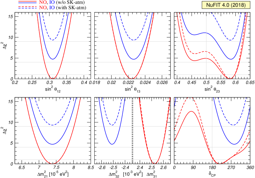
Figure 1: Global $3\nu$ oscillation analysis. The red (blue) curves are for Normal (Inverted) Ordering. Results for different assumptions concerning the analysis of data from reactor experiments are shown as explained in the text.

The table shows that the determination of the leptonic parameters requires global analysis of the data from the differnt experiments. Over the years these analysis have been in the hands of a few phenomenological groups. The results I summarize here are from the updated analysis in Ref. [14] . In Fig. 1 I show the determination of the six parameters from that analysis.

Defining the $3\sigma$ relative precision of the parameter by $2(x^{\rm up}-x^{\rm low})/(x^{\rm up}+x^{\rm low})$, where $x^{\rm up}$ ($x^{\rm low}$) is the upper (lower) bound on a parameter $x$ at the $3\sigma$ level, one reads the following $3\sigma$ relative precision (marginalizing over ordering) :

$$\begin{array}[]{l@{\,,\qquad}l@{\,,\qquad}l}14\%\,(\theta_{12})&8.9\%\,(\theta_{13})&27\,[24]\%\,(\theta_{23})\,,\\ 16\%\,(\Delta m^{2}_{21})&7.8\,[7.6]\%\,(|\Delta m^{2}_{3\ell}|)&100\,[92]\%\,(\delta_{\rm CP})\,,\\ \end{array}$$ (5)

where the numbers between brackets show the impact of including Super-Kamiokande atmospheric resutls (SK-atm) in the precision of that parameter determination (I will comment more on this point in Sec. 2.4). We notice that as $\Delta\chi^{2}$ shape for $\delta_{\rm CP}$ is clearly not gaussian this evaluation of its “precision” can only be taken as indicative. We see that the most unclear issues are: the mass ordering discrimination, the determination of $\sin^{2}\theta_{23}$, and the leptonic CP phase $\delta_{\rm CP}$. In brief:

$\bullet$ The best fit is for the normal mass ordering. Inverted ordering is disfavoured with a $\Delta\chi^{2}=4.7\,(9.3)$ without (with) SK-atm.

$\bullet$ Preference for the second octant of $\theta_{23}$, with the best fit point located at $\sin^{2}\theta_{23}=0.58$. Values with $\sin^{2}\theta_{23}\leq 0.5$ are disfavoured with $\Delta\chi^{2}=4.4\,(6.0)$ without (with) SK-atm.

$\bullet$ The best fit for the complex phase is at $\delta_{\rm CP}=215^{\circ}$. The CP conserving value of $180^{\circ}$, which now is only disfavoured with $\Delta\chi^{2}=1.5$ (1.8) without (with) SK-atm.

2 The Main Track History: Construction of the 3$\nu$ Paradigm

2.1 My Prehistory: Before mid 1990’s

After describing where we are at the present, we need to decide where we start our look to the past. The topic of my talk was the history of the determination of neutrino properties from combined data analysis. As for me the goal of such analysis is to provide that determination in a statistically meaningful manner, I searched for the first time in which neutrino flavour transition data was used in such a way, and the first mass-mixing allowed region were presented. The first paper I found with such a plot was Bellotti etal [15] from 1976 which, interpreting Gargamelle data in terms of the non observation of $\nu_{\mu}\rightarrow\nu_{e}$ oscillation (though this was not an article signed as the experimental collaboration), obtained an exclusion plot on some $\Delta m^{2}$ and mixing angle $\alpha$ with some CL, which I show in Fig. 2 (the main difference with our present plots is the use of the variables $M\equiv\sqrt{\Delta m^{2}}$ and $\sqrt{\sin^{2}2\alpha}$).

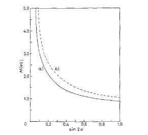
Figure 2: First oscillation parameter plot[15]? (the regions shown at 68% (a) and 95% (b) CL).

By the 80’s such plots had become customary to present the results of the reactor and neutrino fix target experiments. At that time the data was not precise enough to allow for what I would consider global analysis of the experimental results in the statistical sense I defined above. But that did not prevent phenomenologist of the time to search for possible values of neutrino parameters which could somehow describe the bulk of experimental results. I show in my slide in Fig. 3 two examples of such type of studies from Refs.[16, 17]. Besides the audacity behind these efforts, I found interesting that in both cases one of the mass differences pointed out towards ${\cal O}$ (eV) mass scale (see in particular the oscillation parameter region on the right). Looking at what experimental result was driving this, I found that already the early reactor neutrino data was interpreted as a hint (latter on withdraw [4]) of ${\cal O}$ (eV²) neutrino oscillations. In the last years a reactor neutrino anomaly has been suggested which points towards the same scale and it is one of the pillars of the present $eV$ sterile neutrino constructions which I will discuss in Sec. 3.3. There is nothing new under the Sun.

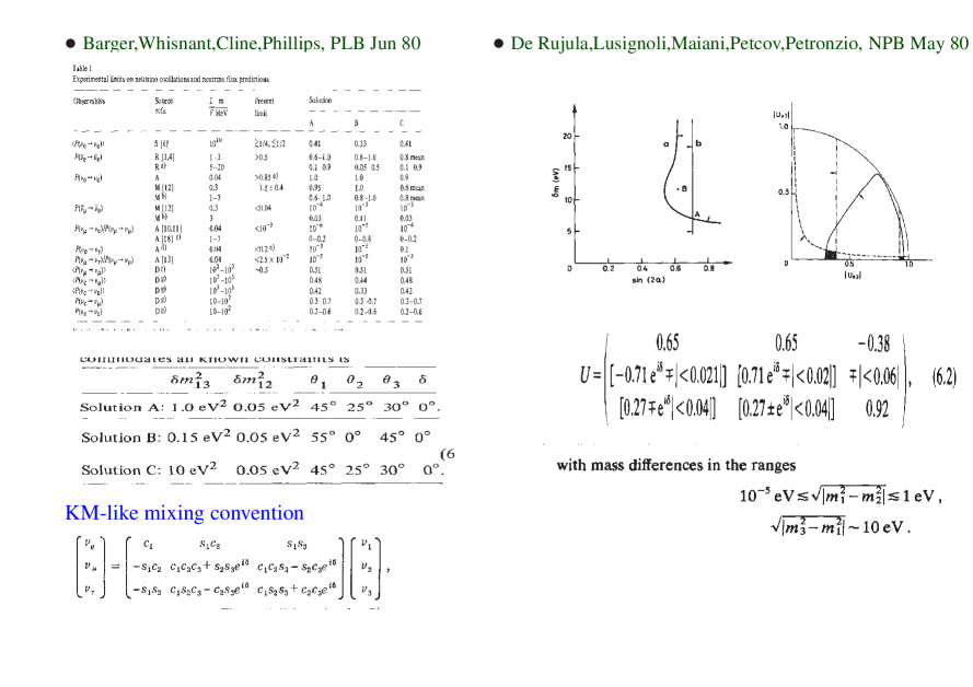
Figure 3: Examples of early global descriptions of oscillation results in Ref. [16] (left) and Ref. [17] (right).

As for what I would consider proper global/combined analysis, at the time I entered into the field, mid 90’s, the state of the art was the 3$\nu$ analysis of Fogli and Lisi [18] which I devotedly studied as my way of learning the subject .

I was lucky enough to enter into the field right at the time when the experimental results which established beyond doubt mass-induced neutrino oscillations started to pour in. In what follows I will try to illustrate the progress we made in the determination of the neutrino parameters as more data came in, by classifying the results by the parameter sectors in the 3$\nu$ oscillation framework.

2.2 Progress by Sectors: $\Delta m^{2}_{21}$ and $\theta_{12}$

As seen in table 1, within the convention we have chosen, $\Delta m^{2}_{12}$ and $\theta_{12}$ are dominantly determined by solar neutrino experiments and KamLAND long baseline reactor data. This is probably the sector where the historical progress in the parameter determination is more striking. I have plotted in the slide in Fig. 4 the parameter plots in this sector presented in a selection of consecutive references from different groups together with the data included in each analysis[21, 22, 23, 24, 25, 26, 27, 28, 29, 30].

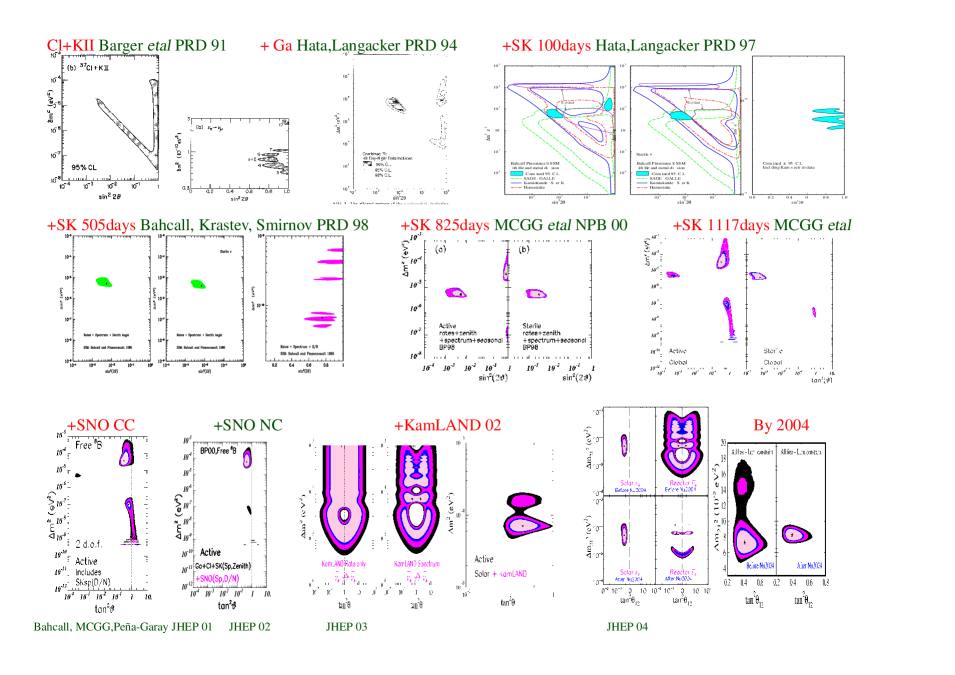
Figure 4: Slide with compilation of the parameter determination in the solar sector with figures taken from Refs. [21, 22, 23, 24, 25, 26, 27, 28, 29, 30]

From the top row we see how the four distinct parameter regions for $\nu_{e}$ oscillations into active neutrinos (any combination of $\nu_{\mu}$ and $\nu_{\tau}$) emerged in the analysis of the solar neutrino data at the time: small mixing angle (SMA, with $\Delta m^{2}\sim 10^{-5}$ eV², $\sin^{2}2\theta\sim 10^{-2}$–$10^{-3}$), large mixing angle (LMA, with $\Delta m^{2}\sim 10^{-4}$ eV², $\sin^{2}2\theta\sim 0.5$–$1$), low mass (LOW with $\Delta m^{2}\sim 10^{-7}$ eV², $\sin^{2}2\theta\sim 1$) and vacuum (or just-so, with $\Delta m^{2}\sim 10^{-10}$ eV², $\sin^{2}2\theta\sim 0.5$–$1$). Oscillations into pure sterile neutrinos were also considered. The modified matter potential for $\nu_{e}\rightarrow\nu_{s}$ implied that they only could lead to a good global description of the solar data with SMA parameters. With the arrival of Super-Kamiokande day-night and spectral data (see second row) the situation became a bit unclear for the first two years as first SMA seemed favoured but soon latter LMA started giving a better fit, more and more so as more statistics was accumulated. In the third row we see how SNO, first CC and then NC data – besides establishing in a total model independent way the solar neutrino flavour transition – when included in the global analysis definitively disfavoured SMA below 3$\sigma$ (and also $\nu_{e}$ oscillations into pure sterile states) allowing only for some small LOW and quasi-vacuum regions at that CL besides LMA. Along then came the first results from the long baseline reactor experiment KamLAND, and, as seen in the last plot, by 2004 a unique allowed range for these two parameters was well established.

Since 2004 the improvement in the determination of $\Delta m^{2}_{21}$ and $\theta_{12}$ has been comparatively modest. Historically, however the comparison of solar and KamLAND data also played a role as giving the first hint towards a non-zero value of $\theta_{13}$ [32] as I will discuss next.

2.3 Progress by Sectors: $\theta_{13}$

I have compiled in the slide in Fig. 5 some plots illustrating the time evolution of the determination of $\theta_{13}$.

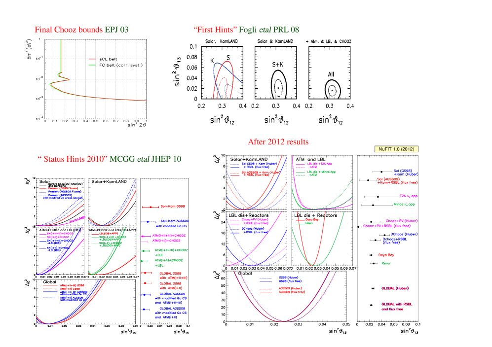
Figure 5: Slide illustrating the the determination of $\theta_{13}$ with figures taken from Refs. [31, 32, 33, 34].

For years our most precise information on $\theta_{13}$ was the upper bound derived from the non-observation of reactor $\bar{\nu}_{e}$ disappearance at short distances. The stringiest bound, shown in the first panel of that figure was provided by the CHOOZ experiment [31]. Within their precision the best fit corresponded to $\theta_{13}$=0. With the known hierarchy between the oscillation wavelengths, setting $\theta_{13}=0$ allowed for the simplification of the 3$\nu$ analysis. For example the survival probability of solar and KamLAND neutrinos in the framework of three neutrino oscillations can be written as:

$$P^{3\nu}_{ee}=\sin^{4}\theta_{13}+\cos^{4}\theta_{13}P^{2\nu}_{ee}(\Delta m^{2}_{21},\theta_{12})\,,$$ (6)

where we have used the fact that $L^{\text{osc}}_{31}=4\pi E/\Delta m^{2}_{31}$ is much shorter than the distance traveled by ether Solar or KamLAND neutrinos, and for solar neutrinos $P^{2\nu}_{ee}(\Delta m^{2}_{21},\theta_{12})$ should be calculated taking into account the evolution in an effective matter density $n^{\text{eff}}_{e}=n_{e}\cos^{2}\theta_{13}$. So for $\theta_{13}=0$ the results obtained within the 3$\nu$ mixing and 2$\nu$ mixing were exactly the same.

However with the more precise data from both solar and KamLAND experiments, the results obtained within the framework of 2$\nu$ oscillation started showing some mismatch between the best fit value of $\theta_{12}$ in solar analysis vs the one obtained in KamLAND which preferred a somewhat larger value. Agreement could be restored with a non-zero value of $\theta_{13}$ because $P^{2\nu}_{ee}(\Delta m^{2}_{21},\theta_{12})$ presents the following asymptotic behaviors

$$P^{2\nu}_{ee}(\Delta m^{2}_{21},\theta_{12}) \simeq 1-\frac{1}{2}\sin^{2}(2\theta_{12}) {\rm for\;solar\;with}\quad E_{\nu} \lesssim{\rm few}\times 100\leavevmode\nobreak\ {\rm KeV}$$

$$P^{2\nu}_{ee}(\Delta m^{2}_{21},\theta_{12}) \simeq\sin^{2}(\theta_{12}) {\rm for\;solar\;with}\quad E_{\nu} \gtrsim{\rm few}\times 1\leavevmode\nobreak\ {\rm MeV}$$

$$P_{ee}^{2\nu}(\Delta m^{2}_{21},\theta_{12}) =1-\frac{1}{2}\sin^{2}(2\theta_{12})\sin^{2}\frac{\Delta m^{2}_{21}L}{2E} {\rm for\;KamLAND}\quad\>.$$

So to obtain the same survival probability with a non-zero value of $\theta_{13}$ at KamLAND $\theta_{12}$ should shift to lower values while the solar region however remains pretty much at the same values of $\theta_{12}$. This is illustrated in the triptych on the upper right of Fig. 5 taken from Ref. [32]. In our 2010 analysis [33] we found that the effect was, however, not very statistically significant as seen in the compilation of the determination of $\theta_{13}$ in the lower left panels of Fig. 5.

The situation became totally clear by 2012 with the results from T2K and specially from the medium baseline reactor experiments, Daya-Bay, Reno and Double-Chooz. In these experiments the dominant oscillation has wavelength determined by $|\Delta m^{2}_{31}|$ and amplitude $\sin^{2}(2\theta_{13})$ (see Eq. (8)). As seen in the panels in the lower right of Fig. 5 [34] in less than one year of data from dedicated experiments the determination of a non-zero $\theta_{13}$ was an uncontroversial $\sim 10\sigma$ effect.

2.4 Progress by Sectors: $\Delta m^{2}_{23}$ and $\theta_{32}$

As seen in table 1, within the convention we have chosen, $|\Delta m^{2}_{23}|$ and $\theta_{23}$ are dominantly determined at present by a combination of atmospheric, LBL and most recently the MBL reactor experiments. I have illustrated in Fig. 6 how the allowed regions for these parameters have changed in the last 20 years.

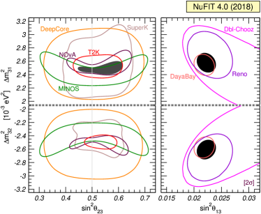
M.C G-G etal PRD Jun 98

Figure 6: Slide illustrating the parameter determination in the atmospheric sector.

The year 1998 holds a special historical significance for neutrino oscillation physics as it was the year in which Super-Kamiokande presented the first evidence of zenith (and therefore distance) dependence of atmospheric multi-GeV $\nu_{\mu}$ disappearance [7]. From the point of view of parameter determination, already with the data at the time it was possible to rule out $\nu_{\mu}\rightarrow\nu_{e}$ as the dominant oscillation channel for $\nu_{\mu}$ disappearance because its corresponding amplitude was determined by the $\theta_{13}$ angle which was already constrained to be too small by CHOOZ. The angular dependence of the event rates also disfavoured oscillations into sterile neutrinos for which matter effects yield a flatter zenith angle dependence. Consequently $\nu_{\mu}\rightarrow\nu_{\tau}$ was established as the dominant flavour transition channel observed in atmospheric oscillations. The relevant survival probability takes the form

$$P_{\mu\mu}\simeq 1-(c_{13}^{4}{\sin^{2}2\theta_{23}}+s_{23}^{2}\sin^{2}2\theta_{13})\sin^{2}\left(\frac{{\Delta m^{2}_{31}}L}{4E}\right)+{\cal O}(\Delta m^{2}_{21})\,.$$ (7)

Therefore in the limit $\theta_{13}=0$ and $\Delta m^{2}_{21}=0$ the atmospheric data analysis determines $|\Delta m^{2}_{31}|=|\Delta m^{2}_{32}|$ and $\sin^{2}(2\theta_{23})$ as shown in the left panels in Fig. 6. Experiments on the most left panel did not provided zenith angle dependence information and therefore the allowed region extended to arbitrary large $\Delta m^{2}$. At the time also some experiments reported an effect while others did not [2, 3].

In the early years of this century, long baseline accelerator experiments, starting with K2K and MINOS confirmed this picture. Furthermore the analysis of their $\nu_{\mu}$ disappearance energy spectrum provided us with the most precise determination of the mass splitting. Precision now is in hands of T2K and NO$\nu$A as seen in Fig. 5.

The latest contribution to the determination of this mass splitting has come in the last five years from the analysis of the spectrum of $\bar{\nu}_{e}$ disappearance in MBL reactor experiments. The relevant survival probability can be approximated as

$$P_{ee}\simeq 1-{\sin^{2}2\theta_{13}}\sin^{2}\left(\frac{{\Delta m^{2}_{ee}}L}{4E}\right)-c_{13}^{4}\sin^{2}2\theta_{12}\sin^{2}\left(\frac{\Delta m^{2}_{21}L}{4E}\right)\;\;$$ (8)

with $\Delta m^{2}_{ee}\simeq|{\Delta m^{2}_{32}}|\pm{c_{12}^{2}\Delta m^{2}_{21}}\simeq|{\Delta m^{2}_{32}}|$. As seen in Fig. 5 the precision attainable on the mass splitting from the analysis of $\bar{\nu}_{e}$ disappearance spectrum at MBL reactor experiments is at present comparable from that of $\nu_{\mu}$ disappearance at LBL accelerator experiments.

In what respects the determination of $\theta_{23}$, till recently it was dominated by the analysis of SK atmospheric neutrinos and it favoured maximal mixing. This changed with the increase precision of the LBL experiments though in not a totally consistent direction. The status on the maximality of $\theta_{23}$, or on the octact preference in case of not maximality, has varied over the last years as more data was gathered. This is still an unsettled issue.

2.5 Ordering and $\delta_{\rm CP}$

There is not much history on the determination of the mass ordering and the CP phase. It is being written as I type these proceedings. The measurement of a not-too-small $\theta_{13}$ made it possible to obtain some statistical significance on both from the analysis of $\nu_{e}$ and $\bar{\nu}_{e}$ appearance in the present LBL experiments, T2K and NO$\nu$A. The quest is on.

An additional issue which has come out over the recent years in this respect, is that of how to include in the global analysis the results of SK-atm on these effects. With the phenomenological tools developed to analyze the data and obtain the results on the dominant effects described above (ie on $\theta_{23}$ and $|\Delta m^{2}_{31}|$), very limited sensitivity to the $\theta_{13}$, the ordering and to $\delta_{\rm CP}$ is found. But the collaboration has developed a more sophisticated analysis method with the aim of constructing enriched samples which are most sensitive to these subdominant effects, and which cannot be technically reproduced outside of the collaboration. Super-Kamiokande has published the results of that analysis in the form of a tabulated $\chi^{2}$ map as a function of the four relevant parameters $\Delta m^{2}_{3\ell},\theta_{23},\theta_{13}$, and $\delta_{\rm CP}$. At the moment this is what is being blindly added in the combined phenomenological analysis. As seen in Fig. 1 this addition has a non-negligible impact on the statistical discrimination between orderings (and somewhat less on the determination of $\delta_{\rm CP}$).

2.6 The Neutrino Mass Scale

Oscillation experiments provide information on $\Delta m^{2}_{ij}$, and on the leptonic mixing angles, $U_{ij}$. But they are insensitive to the absolute mass scale for the neutrinos. Of course, the results of an oscillation experiment do provide a lower bound on the heavier mass in $\Delta m^{2}_{ij}$, $|m_{i}|\geq\sqrt{\Delta m^{2}_{ij}}$ for $\Delta m^{2}_{ij}>0$. But there is no upper bound on this mass. In particular, the corresponding neutrinos could be approximately degenerate at a mass scale that is much higher than $\sqrt{\Delta m^{2}_{ij}}$. Moreover, there is neither upper nor lower bound on the lighter mass $m_{j}$.

The only model independent information on the neutrino masses, rather than mass differences, can be extracted from kinematic studies of reactions in which a neutrino or an anti-neutrino is involved. Historically these bounds were labeled as limits on the mass of the flavour neutrino states corresponding to the charged flavour involved in the decay:
                    $m_{\nu_{e}}\leq 2.2\,{\rm eV}$ From ${\rm{}^{3}H\rightarrow\ ^{3}He+e^{-}+\overline{\nu}_{e}}$ [35]                     $m_{\nu_{\mu}}\leq 0.19\,{\rm MeV}$ From ${\rm\pi\rightarrow\mu+\nu_{\mu}}$ [36]                     $m_{\nu_{\tau}}\leq 10.2\,{\rm MeV}$ From ${\rm\tau\rightarrow{\rm N}\pi^{\prime}s+\nu_{\tau}}$ [36]

In the presence of mixing the bounded combinations are indeed

$$m_{\nu_{\alpha}}^{2}=\sum_{i}|U_{\alpha i}|^{2}m_{i}^{2}\;,$$ (9)

so with the values known of the mixing matrix elements the most relevant constraint comes from Tritium beta decay and it has been standing at the value of 2.2 eV for almost two decades. It is expected to be superseded by KATRIN which will improve the sensitivity by about one order of magnitude.

Model dependent information on neutrino masses can also be obtained from neutrinoless double beta decay $(A,Z)\rightarrow(A,Z+2)+e^{-}+e^{-}$. This process is the most sensitive test of the Dirac vs Majorana nature of the neutrinos. If they are Majorana particles and in the context of the NMSM (in which no other source of lepton number violation is present in the model) the rate of this process is proportional to the effective Majorana mass of $\nu_{e}$,

$$m_{ee}=\left|\ \ \sum_{i}m_{i}U_{ei}^{2}\ \ \right|$$ (10)

which, depends also on the three CP violating phases. Notice that in order to induce the $2\beta 0\nu$ decay, $\nu$’s must Majorana particles, thus if neutrinos are Dirac particles no information on their masses can be deduced from the non-observation of $2\beta 0\nu$ decay. As we heard in the talk of S. Petcov [37] at present the most stringent bounds are $m_{ee}\leq 0.06$–$0.4$ where the range spans over the nuclei involved as well as the expected uncertainty associated with the nuclear matrix model.

Neutrinos, like any other particles, contribute to the total energy density of the Universe and have impact in its evolution [38]. Within what we presently know of their masses, neutrinos are relativistic through most of the evolution of the Universe and being very weakly interacting they decoupled early in cosmic history. Depending on their exact masses they can impact the CMB spectra, in particular by altering the value of the redshift for matter-radiation equality. More importantly, their free streaming suppresses the growth of structures on scales smaller than the horizon at the time when they become non-relativistic and therefore affects the matter power spectrum which is probed from surveys of the LSS distribution. Within their present precision, cosmological observations are sensitive to neutrinos mostly via their contribution to the energy density in our Universe, $\Omega_{\nu}h^{2}=\sum_{i}m_{i}/(94\,{\rm eV})$. Therefore cosmological data mostly gives information on the sum of the neutrino masses and has very little to say on their mixing structure and on the ordering of the mass states. At present the most robust bounds come from the analysis of Planck results which within the $\Lambda$-CDM model imply $\sum_{i}m_{i}\leq 0.17-0.74$ eV where the range includes variations of the data sets included in the analysis. One must always keep in mind that these bounds apply within a given cosmological model. Variations of the model can relax the bounds.

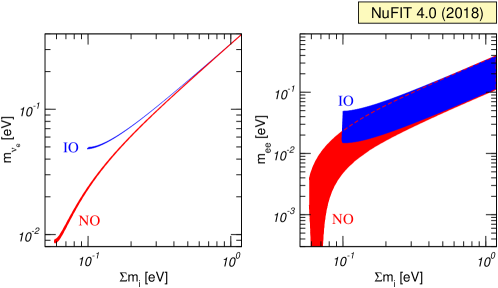
Figure 7: 95% allowed regions (for 2 dof) in the planes ($m_{\nu_{e}}$,$\sum m_{\nu}$) and ($m_{ee}$,$\sum m_{\nu}$) from the global analysis of oscillation data (full regions).

Within the 3$\nu$ scenario, correlated information on the three probes of neutrino masses can be obtained by mapping the results from the global analysis of oscillations presented in the previous section [39]. I show in Fig. 7 the updated status of this exercise. The narrow range observed in the left panel corresponds to the uncertainty associated with the present determination of oscillation parameters, which, as seen in the figure, is rather small. On the contrary the wide range observed in the right panel corresponds to the effect of the unknown Majorana phases. From the figure one can infer that a positive determination of two of these probes (or a sufficiently strong bound) could help to determine the ordering of the states, and give some information about the Majorana phases within the corresponding model assumptions. In this front, the quest is also ongoing with claims and disclaims on the significance of the effects being observed.

3 The Parallel Paths

While the consistency of the minimal picture of mass-induced 3$\nu$ oscillations was being established, other scenarios – either alternative or extentended – were proposed and as such were confronted with the data to learn about their relevant parameters. One can consider those scenarios as parallel paths that our history could have chosen to follow and in this section I am going to briefly describe some of them.

3.1 Alternative Scenarios for Flavour Conversion in Vacuum

Oscillations are not the only possible mechanism for neutrino flavour transitions and over the years alternative scenarios were proposed with nonstandard neutrino physics characterized by the presence of an unconventional interaction (other than the neutrino mass terms) that mixes neutrino flavours. From the point of view of neutrino oscillation phenomenology, a critical feature of these scenarios is a departure from the $\lambda\propto E/\Delta m^{2}$ dependence of the conventional oscillation wavelength and instead $\lambda\propto E^{-n}/\Delta\delta$ where $n$ and $\delta$ depends on the specific mechanism. Examples include:

$\bullet$ Violation of the equivalence principle [40], due to non- universal coupling of the neutrinos, $\gamma_{1}\neq\gamma_{2}$ to the local gravitational potential $\phi$, or breakdown of Lorentz invariance  [41, 42]resulting from different asymptotic values of the velocity of the neutrinos, $c_{1}\neq c_{2}$, for which $n=1$

$\bullet$ Non-universal coupling of the neutrinos, $k_{1}\neq k_{2}$ to a space-time torsion field $Q$ [43] or Violation of CPT resulting from Lorentz-violating effects such as the operator, $\bar{\nu}_{L}^{\alpha}b_{\mu}^{\alpha\beta}\gamma_{\mu}\nu_{L}^{\beta}$,  [44, 45, 46] which lead to an energy independent contribution to the oscillation wavelength.

Atmospheric neutrinos with their broad energy range and travel distances are the ideal probe for these type of scenarios and already with the early data from Super-Kamiokande it was possible to rule them out as the dominant mechanism responsible for the observed flavour transitions [47]. Furthermore as data from LBL experiments became available it was possible to constraint the subdominant contribution from these scenarios to the standard 3$\nu$ oscillation transitions and impose severe bounds on these extensions of the NMSM, for example[48]

$$\begin{array}[]{ll}\Delta\delta=2|\phi|(\gamma_{1}-\gamma_{2})\leq 1.6\times 10^{-24}\,,&\qquad{\rm for\,VEP}\\ \Delta\delta=(c_{1}-c_{2})\leq 1.6\times 10^{-24}\,,&\qquad{\rm for\,VLI}\\ \Delta\delta=Q(k_{1}-k_{2})\leq 6.3\times 10^{-23}\leavevmode\nobreak\ {\rm GeV}\,,&\qquad{\rm for\,coupling\,to\,torsion}\\ \Delta\delta=b_{1}-b_{2}\leq 5.0\times 10^{-23}\leavevmode\nobreak\ {\rm GeV}\,\,,&\qquad{\rm for\,\,\,/\!\!\!\!\!CPT\,,\,VLI}\;.\end{array}$$ (11)

3.2 Non-standard Neutrino Interactions

A mechanism for flavour transitions which is not fully described by the above formalism is that of non-standard neutrino interactions (NSI) with matter. In particular neutral current NSI’s can impact the coherent scattering of neutrinos in matter. Neutral current NSI’s can be parametrized by effective four-fermion operators of the form

$$\mathcal{L}_{\rm NSI}=-2\sqrt{2}G_{F}\varepsilon_{\alpha\beta}^{fP}(\bar{\nu}_{\alpha}\gamma^{\mu}L\nu_{\beta})(\bar{f}\gamma_{\mu}Pf)\,,$$ (12)

where $f=e,u,d$ is a charged fermion, $P=(L,R)$ and $\varepsilon_{\alpha\beta}^{fP}$ are dimensionless parameters encoding the deviation from standard interactions. These operators contribute to the effective matter potential in the Hamiltonian describing the evolution of the neutrino flavour state:

$$H_{\text{mat}}=\sqrt{2}G_{F}N_{e}(x)\begin{pmatrix}1+\epsilon_{ee}&\epsilon_{e\mu}&\epsilon_{e\tau}\\ \epsilon_{e\mu}^{*}&\epsilon_{\mu\mu}&\epsilon_{\mu\tau}\\ \epsilon_{e\tau}^{*}&\epsilon_{\mu\tau}^{*}&\epsilon_{\tau\tau}\end{pmatrix},\;\;{\rm with}\;\;\epsilon_{\alpha\beta}(x)=\sum_{f=e,u,d}\frac{N_{f}(x)}{N_{e}(x)}\epsilon_{\alpha\beta}^{f,V}\,,$$ (13)

with $N_{f}(x)$ being the density of fermion $f$ along the neutrino path. The “1” in the $ee$ entry in Eq. (13) corresponds to the standard MSW matter potential. Therefore, the effective NSI parameters entering oscillations, $\epsilon_{\alpha\beta}$, may depend on $x$ and will be generally different for neutrinos crossing the Earth or the solar medium and as such can be constrained by the global analysis of neutrino oscillation data (since oscillation experiments are only sensitive to differences between the diagonal terms in the matter potential).

The task becomes troubled by an intrinsic degeneracy in the Hamiltonian governing neutrino oscillations which is introduced by the NSI-induced matter potential. In general, CPT implies that neutrino evolution is invariant if the relevant Hamiltonian is transformed as $H\to-H^{*}$. In vacuum this transformation can be realized by changing the oscillation parameters as

$$\Delta m^{2}_{31}\to-\Delta m^{2}_{31}+\Delta m^{2}_{21}=-\Delta m^{2}_{32}\,,\;\;\;\sin\theta_{12}\leftrightarrow\cos\theta_{12}\,,\;\;\;\delta_{\rm CP}\to\pi-\delta_{\rm CP}\,.$$ (14)

In the standard 3$\nu$ oscillation scenario, this symmetry is broken by the standard matter effect, and this allows for the determination of the octant of $\theta_{12}$ and (in principle) of the sign of $\Delta m^{2}_{31}$. However, in the presence of NSI, the symmetry can be restored if in addition to the transformation Eq. (14), NSI parameters are transformed as

$$(\varepsilon_{ee}-\varepsilon_{\mu\mu})\to-(\varepsilon_{ee}-\varepsilon_{\mu\mu})-2\,,\;\;\;(\varepsilon_{\tau\tau}-\varepsilon_{\mu\mu})\to-(\varepsilon_{\tau\tau}-\varepsilon_{\mu\mu})\,,\;\;\;\varepsilon_{\alpha\beta}\to-\varepsilon_{\alpha\beta}^{*}\qquad(\alpha\neq\beta)\,.$$ (15)

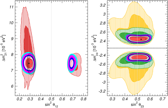
Figure 8: Two-dimensional projections of the allowed regions onto different vacuum parameters (on the right $\Delta m^{2}_{\mu\mu}\simeq\Delta m^{2}_{31}$) after marginalizing over the matter potential parameters and the undisplayed oscillation parameters. The solid colored regions correspond to the global analysis of all oscillation data, and show the $1\sigma$, 90%, $2\sigma$, 99% and $3\sigma$ CL allowed regions; the best fit point is marked with a star. The black void regions correspond to the analysis with the standard matter potential (i.e., without NSI) and its best fit point is marked with an empty dot. For comparison, in the left panel we show in red the 90% and $3\sigma$ allowed regions including only solar and KamLAND results, while in the right panels we show in green the 90% and $3\sigma$ allowed regions excluding solar and KamLAND data, and in yellow the corresponding ones excluding also IceCube and reactor data.

In Fig. 8 I show the two-dimensional projections of the allowed regions onto different sets of oscillation parameters from the global analysis in Ref. [49] in the presence of this generalized matter potential (13). These regions are obtained after marginalizing over the undisplayed vacuum parameters as well as the NSI couplings. For comparison its also shown as black-contour void regions the corresponding results with the standard matter potential, i.e., in the absence of NSI.

From the figure we read the following:

$\bullet$ The determination of the oscillation parameters discussed in the previous section is robust under the presence of NSI as large as allowed by the oscillation data itself with the exception of the octant of $\theta_{12}$. This result relies on the complementarity and synergies between the different data sets, which allows to constrain those regions of the parameter space where cancellations between standard and non-standard effects occur in a particular data set.

$\bullet$ A solution with $\theta_{12}>45^{\circ}$ still provides a good fit. This is the so-called LMA-D solution and it was first found in Ref. [50]. It is is a consequence of the intrinsic degeneracy in the Hamiltonian described above. Eq. (14) shows that this degeneracy implies a change in the octant of $\theta_{12}$ (as manifest in the LMA-D). As such it cannot be ruled out by oscillation data only. Scattering data, in particular from the finally-observed coherent scattering in nuclei [51] disfavoured it at more then 3$\sigma$ for NSI coupling neutrinos with either up or down quarks. But it is still allowed for more general NSI couplings [49].

LMA-D requires large $\varepsilon_{ee}-\varepsilon_{\mu\mu}\sim{\cal O}(2)$ which are therefore still allowed by the global analysis. But for all other couplings the same global analysis sets strong constrains on $\varepsilon_{\alpha\beta}$ yielding the most restrictive bounds on the NSI parameters, in particular those involving $\tau$ flavour.

3.3 Light Sterile Neutrinos

The vast majority of the neutrino data on flavour transitions accumulated over the years could be consistently described in the framework of three neutrino mixing. There appeared, however, a set of anomalies in neutrino data at relatively short-baselines (SBL) which could not. As mentioned before, in the early 1990’s LSND [19] reported the observation of $\nu_{\mu}\rightarrow\nu_{e}$ ( over the last decade it has been tested at MiniBooNE which also found an anomaly though not exactly as expected from LSND [52]). A few years latter it was also pointed out that the $\nu_{e}$ source experiments made to test the efficiency of gallium solar experiments did also saw a deficit compared with expectations [53]. The third set of anomalies arose in $\bar{\nu}_{e}$ reactor experiments as described in Laserre’s talk [9] and came out also as a deficit compared to theoretical expectations. If interpreted in terms of oscillations, each of these anomalies points out towards a $\Delta m^{2}\sim{\cal O}({\rm eV}^{2})$ and consequently cannot be described within the context of the 3$\nu$ mixing described in the previous section. They require, instead, the addition of one or more additional neutrinos which must be sterile, i.e. elusive to Standard Model interactions, to account for the constraint of the invisible $Z$ width which limits the number of light weak-interacting neutrinos to be $2.984\pm 0.008$.

The most immediate question as these anomalies were reported was whether they could all be consistently described in combination with the rest of the neutrino data if one adds those additional sterile states. Quantitatively one can start by adding a fourth massive neutrino state to the spectrum and perform a global analysis to answer this question. Although the answer is always the same the way to come about it depends on the way the massive states are ordered. In brief, there are six possible four-neutrino schemes which can in principle accommodate the results of solar+KamLAND and atmospheric+LBL neutrino experiments as well as the SBL result. They can be divided in two classes: (2+2) and (3+1). In the (3+1) schemes, there is a group of three close-by neutrino masses (as on the 3$\nu$ schemes described in the previous section) that is separated from the fourth one by a gap of the order of 1 ${\rm eV}^{2}$, which is responsible for the SBL oscillations. In (2+2) schemes, there are two pairs of close masses (one pair responsible for solar results and the other for atmospheric [20]) separated by the ${\cal O}({\rm eV}^{2})$ gap. The main difference between these two classes is the following: if a (2+2)-spectrum is realized in nature, the transition into the sterile neutrino is a solution of either the solar or the atmospheric neutrino problem, or the sterile neutrino takes part in both. This makes this spectrum easier to test as the required mixing of sterile neutrinos in either solar and/or atmospheric oscillations will modify their effective matter potential in the Sun and in the Earth and have observable effects in the data. As described in the previous section none of those effects were observed and oscillations into sterile neutrinos did not describe well neither solar nor atmospheric data. Consequently as soon as the early 2000’s 2+2 spectra could be ruled out already beyond 3-4 $\sigma$ as seen in the left panel in Fig. 9 taken from Ref.[54].

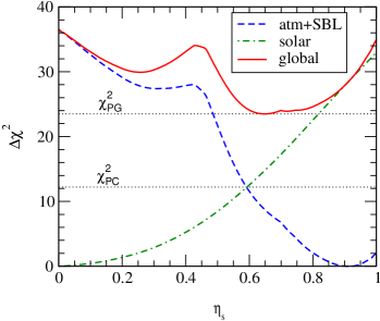
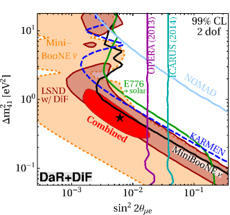
Figure 9: Left: Status of the 2+2 oscillation scenarios from Ref. [54] ($\eta_{S}=\displaystyle\sum_{i}|U_{is}|^{2}$ where $i$ runs over the two massive states mostly relevant for solar neutrino oscillations). Right: Present status of 3+1 oscillation scenarios from Ref. [55].

On the contrary, for a (3+1)-spectrum (indeed 3+N), the sterile neutrino(s) could be only slightly mixed with the active ones and mainly provide a description of the SBL results. Qualitatively the constraints on these scenarios come from the tension between the non-negligible mixing of both $\nu_{e}$ and $\nu_{\mu}$ with the additional massive states required to explain both the LSND/MiniBooNE appearance results and the $\nu_{e}$,$\bar{\nu}_{e}$ disappearance results from Gallium and reactor data, with the constraints on the same mixings from the rest of the data. Again, this is history written as I type with the upcoming of several reactor experiments designed specifically for testing these scenarios. The status of the global analysis of the available data at the time of this talk is illustrated in the right panel in Fig. 9 taken from Ref.[55] which concluded that 3+1 scenario is excluded at 4.7$\sigma$ level. Also quoting from that reference the tension cannot be eliminated by discarding any individual experiment.

4 Epilogue

Human history is mostly told by the winners. But in neutrino physics, and in science in general, I would like to think that we can all consider ourselves winners in one way or another. For me the prize of being an informed witness of the discovery of beyond the Standard Model Physics has certainly been worth the effort of countless white nights, stressful last minute talk updates, and the hundreds of life anecdotes they provoked.

And if that was not enough, it brought me to Paris for this conference to enjoy the company of great people. Above all the organizers to whom I remain indebted for their invitation.

References

References

- [1] T. Kirsten in these proceedings.
- [2] P. Lipari in these proceedings.
- [3] J. Learned in these proceedings.
- [4] P. Vogel in these proceedings.
- [5] K. Kleinkecht in these proceedings.
- [6] G. Feldman in these proceedings.
- [7] T. Kajita in these proceedings.
- [8] A. McDonald in these proceedings.
- [9] T. Laserre in these proceedings.
- [10] A. Smirnov in these proceedings.
- [11] P. Ramond in these proceedings.
- [12] S. Bilenky in these proceedings.
- [13] E. Akhmedov in these proceedings.
- [14] I. Esteban, M. C. Gonzalez-Garcia, A. Hernandez-Cabezudo, M. Maltoni and T. Schwetz, arXiv:1811.05487 [hep-ph].
- [15] E. Bellotti, D. Cavalli, E. Fiorini and M. Rollier, Lett. Nuovo Cim. 17, 553 (1976).
- [16] V. D. Barger, K. Whisnant, D. Cline and R. J. N. Phillips, Phys. Lett. 93B, 194 (1980).
- [17] A. De Rujula, M. Lusignoli, L. Maiani, S. T. Petcov and R. Petronzio, Nucl. Phys. B 168, 54 (1980).
- [18] G. L. Fogli, E. Lisi and D. Montanino, Phys. Rev. D 49, 3626 (1994).
- [19] A. Aguilar-Arevalo et al. [LSND Collaboration], Phys. Rev. D 64 (2001) 112007 [hep-ex/0104049].
- [20] J. J. Gomez-Cadenas and M. C. Gonzalez-Garcia, Z. Phys. C 71, 443 (1996).
- [21] V. D. Barger, R. J. N. Phillips and K. Whisnant, Phys. Rev. D 43, 1110 (1991).
- [22] N. Hata and P. Langacker, Phys. Rev. D 48, 2937 (1993)
- [23] N. Hata and P. Langacker, Phys. Rev. D 56, 6107 (1997)
- [24] J. N. Bahcall, P. I. Krastev and A. Y. Smirnov, Phys. Rev. D 58, 096016 (1998)
- [25] M. C. Gonzalez-Garcia, P. C. de Holanda, C. Pena-Garay and J. W. F. Valle, Nucl. Phys. B 573, 3 (2000)
- [26] M. C. Gonzalez-Garcia and C. Pena-Garay, Nucl. Phys. Proc. Suppl. 91, 80 (2001)
- [27] J. N. Bahcall, M. C. Gonzalez-Garcia and C. Pena-Garay, JHEP 0108, 014 (2001)
- [28] J. N. Bahcall, M. C. Gonzalez-Garcia and C. Pena-Garay, JHEP 0207, 054 (2002)
- [29] J. N. Bahcall, M. C. Gonzalez-Garcia and C. Pena-Garay, JHEP 0302, 009 (2003)
- [30] J. N. Bahcall, M. C. Gonzalez-Garcia and C. Pena-Garay, JHEP 0408, 016 (2004)
- [31] M. Apollonio et al. [CHOOZ Collaboration], Eur. Phys. J. C 27, 331 (2003)
- [32] G. L. Fogli, E. Lisi, A. Marrone, A. Palazzo and A. M. Rotunno, Phys. Rev. Lett. 101, 141801 (2008) [arXiv:0806.2649 [hep-ph]].
- [33] M. C. Gonzalez-Garcia, M. Maltoni and J. Salvado, JHEP 1004, 056 (2010)
- [34] M. C. Gonzalez-Garcia, M. Maltoni, J. Salvado and T. Schwetz, JHEP 1212, 123 (2012)
- [35] J. Bonn, et al., Nucl. Phys. Proc. Suppl. 91, 273 (2001); V.M. Lobashev, et al., Nucl. Phys. Proc. Suppl. 91, 280 (2001).
- [36] M. Tanabashi et al. [Particle Data Group], Phys. Rev. D 98, no. 3, 030001 (2018).
- [37] S. Petcov in these proceedings.
- [38] J. Rich in these proceedings.
- [39] G. L. Fogli et al., Phys. Rev. D 70 (2004) 113003
- [40] M. Gasperini, Phys. Rev. D 38 (1988) 2635; Phys. Rev. D 39, 3606 (1989);
- [41] S. Coleman and S.L. Glashow, Phys. Lett. B 405, 249 (1997).
- [42] S.L. Glashow, A. Halprin, P.I. Krastev, C.N. Leung, and J. Pantaleone, Phys. Rev. D 56, 2433 (1997).
- [43] V. De Sabbata and M. Gasperini, Nuovo Cimento A 65, 479 (1981).
- [44] D. Colladay and V.A. Kostelecky, Phys. Rev. D55, 6760 (1997).
- [45] S. Coleman and S.L. Glashow, Phys. Rev. D 59, 116008 (1999).
- [46] V. D. Barger, S. Pakvasa, T. J. Weiler and K. Whisnant, Phys. Rev. Lett. 85, 5055 (2000)
- [47] G. L. Fogli, E. Lisi, A. Marrone and G. Scioscia, Phys. Rev. D 60, 053006 (1999)
- [48] M. C. Gonzalez-Garcia and M. Maltoni, Phys. Rev. D 70, 033010 (2004).
- [49] I. Esteban, M. C. Gonzalez-Garcia, M. Maltoni, I. Martinez-Soler and J. Salvado, JHEP 1808, 180 (2018) [arXiv:1805.04530 [hep-ph]].
- [50] O. G. Miranda, M. A. Tortola and J. W. F. Valle, JHEP 0610, 008 (2006) [hep-ph/0406280].
- [51] D. Akimov et al. [COHERENT Collaboration], Science 357, no. 6356, 1123 (2017) [arXiv:1708.01294 [nucl-ex]].
- [52] A. A. Aguilar-Arevalo et al. [MiniBooNE DM Collaboration], Phys. Rev. D 98, no. 11, 112004 (2018) [arXiv:1807.06137 [hep-ex]].
- [53] M. A. Acero, C. Giunti and M. Laveder, Phys. Rev. D 78 (2008) 073009 [arXiv:0711.4222 [hep-ph]].
- [54] M. Maltoni, T. Schwetz, M. A. Tortola and J. W. F. Valle, Nucl. Phys. B 643, 321 (2002) [hep-ph/0207157].
- [55] M. Dentler, Á. Hernández-Cabezudo, J. Kopp, P. A. N. Machado, M. Maltoni, I. Martinez-Soler and T. Schwetz, JHEP 1808 (2018) 010 [arXiv:1803.10661 [hep-ph]].