The Fe II/Mg II flux ratio of low-luminosity quasars at z $\sim$3

Abstract

The Fe II/Mg II line flux ratio has been used to investigate the chemical evolution of high redshift active galactic nuclei (AGNs). No strong evolution has been found out to $z\sim 6$, implying that the type 1a supernova activity has been already occurred in early universe. However, the trend of no evolution can be caused by the sample selection bias since the previous studies have utilized mostly very luminous AGNs, which may be already chemically matured at the observed redshift. As motivated by the previously reported correlation between AGN luminosity and metallicity, we investigate the Fe II/Mg II flux ratio over a large dynamic range of luminosity, by adding a new sample of 12 quasars at $z\sim 3$, of which the lower luminosity limit is more than 1 dex smaller than that of the previously studied high-z quasars. Based on the Gemini/GNIRS observations, we find that the seven low-luminosity quasars with a mean bolometric luminosity log $L_{\rm bol}\sim 46.5\pm 0.2$ has an average Fe II/Mg II ratio of $0.68\pm 0.11$ dex. This ratio is comparable to that of high-luminosity quasars (log $L_{\rm bol}\sim 47.3\pm 0.3$) in our sample (i.e., Fe II/Mg II ratio of $0.59\pm 0.15$ dex) and that of the previously studied high-luminosity quasars at higher redshifts. One possible scenario is that the low-luminosity quasars in our sample are still relatively luminous and already chemically matured. To search for chemically-young AGNs, and fully understand the chemical evolution based on the Fe II/Mg II/ flux ratio, it is required to investigate much lower-luminosity AGNs.

I. INTRODUCTION

Chemical properties of galaxies are powerful diagnostics in understanding galaxy evolution since the chemical composition is determined by the star-formation history as well as the gas inflow and outflow. As the metallicity measurements of galaxies at high redshifts are particularly interesting for exploring the early phase of galaxy evolution, the gas phase metallicity of star-forming galaxies has been measured even at $z>3$ (e.g., Maiolino et al., 2008; Mannucci et al., 2009; Nagao et al., 2012; Amorín et al., 2014; Troncoso et al., 2014; Sanders et al., 2016; Onodera et al., 2016; Shapley et al., 2017). However, such metallicity measurements are generally very challenging due to the faintness of star-forming galaxies at high-z. Alternatively active galactic nuclei (AGNs) powered by a supermassive black hole (SMBH) have been utilized for inferring the chemical composition of galaxies in the early Universe, owing to their high apparent magnitude as well as numerous metallic emission lines seen in the rest-frame ultraviolet (UV) spectra.

It has been pointed out through theoretical simulations that various combinations of broad emission lines observed in the UV spectra of quasars (especially with the N V$\lambda$1240 line, i.e., N V$\lambda$1240/C IV$\lambda$1549 and N V$\lambda$1240/He II$\lambda$1640; hereafter N V/C IV and N V/He II) are useful to infer the gas metallicity of broad-line regions (BLRs) in quasars (e.g., Hamann & Ferland, 1992, 1993; Nagao et al., 2006b). By using these flux ratios, a positive correlation between AGN luminosity and the BLR metallicity has been reported (e.g., Hamann & Ferland, 1993; Shemmer & Netzer, 2002; Shemmer et al., 2004; Warner et al., 2004; Nagao et al., 2006b; Shin et al., 2013). This correlation can be interpreted as the result of the underlying correlation between the mass of SMBHs ($M_{\rm BH}$) and the BLR metallicity (Warner et al., 2003, 2004; Matsuoka et al., 2011b), at least in the high-redshift Universe as AGN luminosity roughly scales with $M_{\rm BH}$ (but see also Shin et al. 2013 for low-z AGNs). Since $M_{\rm BH}$ is tightly correlated with the mass of the spheroidal component of galaxies (e.g., Magorrian et al., 1998; Ferrarese & Merritt, 2000; Gebhardt et al., 2000; Marconi & Hunt, 2003; Häring & Rix, 2004; Kormendy & Ho, 2013; Woo et al., 2013, 2015), it is possible to interprete that the AGN luminosity-BLR metallicity correlation in quasars is caused by the mass-metallicity relation of galaxies (e.g., Lequeux et al., 1979; Tremonti et al., 2004). In other words, more massive galaxies with higher gas metallicity host more massive black holes, which are observed as on-average higher-luminosity AGNs, if we assume the Eddington ratio distribution is similar, regardless of the mass scale.

Surprisingly, studies of the BLR metallicity based on N V/C IV using quasars over a wide range of redshift have found no metallicity evolution out to $z\sim 4$ or even higher redshift (e.g., Nagao et al. 2006b; Matsuoka et al. 2011b; Xu et al. 2018 ; see also Juarez et al. 2009; De Rosa et al. 2014; Mazzucchelli et al. 2017). Note that the gas metallicity of narrow-line regions (NLRs) also shows no redshift evolution (e.g., Nagao et al., 2006a; Matsuoka et al., 2009, 2011a; Dors et al., 2014). These results are unexpected, because the mass-metallicity relation of star-forming galaxies shows a significant redshift evolution toward $z\sim 3$, even for the most massive galaxies (e.g., Maiolino et al. 2008; Troncoso et al. 2014; Onodera et al. 2016; see also Sommariva et al. 2012).

In investigating the chemical evolution of AGNs, the flux ratio of the UV Fe II multiplet emission to the Mg II$\lambda$2800 emission (hereafter Fe II/Mg II) measured from the UV spectra of quasars provides a more interesting diagnostic, since the timescale of the iron enrichment is much longer than other metallic elements. This is because the iron is mainly ejected from the type Ia super novae (SNIa) while the $\alpha$-elements including magnesium are produced mostly by the core-collapse super novae. Thus, the enrichment timescale of magnesium is much shorter than that of iron. Various attempts have been made to identify the redshift where a significant decrease of Fe II/Mg II flux ratio can be detected due to the decrease of the iron abundance relative to magnesium. However, no significant redshift evolution of Fe II/Mg II flux ratio has been observed out to $z\sim 7$ (e.g., Barth et al., 2003; Dietrich et al., 2003; Maiolino et al., 2003; Iwamuro et al., 2004; Jiang et al., 2007; Kurk et al., 2007; De Rosa et al., 2011; Mazzucchelli et al., 2017). One potential explanation of this mystery is the sample bias. The previous studies have used mainly high-luminosity quasars (i.e., $L_{\rm bol}\gtrsim 10^{47}$ erg s^-1) at high redshifts for investigating the Fe II/Mg II ratio evolution. Such very luminous quasars, with presumably high mass black holes, are likely to be already chemically matured, as expected from the mass-dependent evolution of galaxies (Juarez et al. 2009; see also Kawakatu et al. 2003).

To explore potential candidates of chemically young quasars, we focus on low-luminosity quasars, that have not been extensively investigated. By measuring the Fe II/Mg II flux ratio of low-luminosity quasars, we aim at shedding light on the chemical evolution of quasars in the early Universe. In §2, we describe the sample and observations. The analysis and results follow in §3 and §4. In §5, we provide the discussion based on the results. We adopt a cosmology of $H_{\rm 0}=70$ km s^-1 Mpc^-1, $\Omega_{\Lambda}=0.7$ and $\Omega_{\rm m}=0.3$.

Table 1Log of observations

Target	RA	Dec	Redshift	$m_{I}$	Observation Date	Exposure	Standard star
	(deg)	(deg)		(mag)		(sec)
(1)	(2)	(3)	(4)	(5)	(6)	(7)	(8)
SDSS J082854.44+571637.2	$127.22686$	$57.27702$	$3.383$	$20.20$	2012 Feb 09	$300\times 32$	HIP 42124 (A5V)
SDSS J124652.80+545140.6	$191.72000$	$54.86130$	$3.360$	$20.11$	2012 Feb 09	$300\times 24$	HIP 61510 (F0V)
SDSS J120308.69+552245.8	$180.78622$	$55.37941$	$3.355$	$20.15$	2012 Feb 09	$300\times 16$	HIP 63153 (F4V)
SDSS J081528.12+344737.0	$123.86720$	$34.79362$	$3.200$	$20.19$	2015 Mar 19	$140\times 36$	HIP 47631 (F3V)
SDSS J095617.14+373224.7	$149.07143$	$37.54022$	$3.245$	$20.38$	2015 Mar 19	$140\times 36$	HIP 51914 (F3V)
SDSS J133600.20+391826.2	$204.00087$	$39.30729$	$3.228$	$20.40$	2015 Mar 20	$140\times 36$	HIP 72469 (F2V)
SDSS J142903.86+062620.4	$217.26610$	$6.43901$	$3.268$	$20.49$	2015 Mar 22	$140\times 36$	HIP 77946 (F0V)
SDSS J010049.76+092936.1	$15.20736$	$9.49337$	$3.118$	$18.65$	2017 Nov 23	$300\times 8$	HIP 06373 (F4V)
SDSS J013735.46–004723.4	$24.39779$	$-0.78983$	$3.209$	$19.26$	2017 Nov 24	$300\times 20$	HIP 01964 (F3V)
SDSS J093514.41+343659.5	$143.81004$	$34.61654$	$3.227$	$18.40$	2017 Nov 24	$300\times 8$	HIP 49548 (F3V)
SDSS J223408.99+000001.6	$338.53748$	$0.00047$	$3.026$	$17.29$	2017 Nov 22	$248\times 4$	HIP 107167 (F2V)
SDSS J231934.77–104037.0	$349.89489$	$-10.67695$	$3.170$	$18.13$	2017 Nov 23	$300\times 8$	HIP 112782 (F0V)

Note. — Col. (4, 5): Redshift and $I$-band model magnitude are taken from SDSS DR12 (Alam et al., 2015). Col. (8): Standard stars used for the telluric absorption correction and the flux calibration. The spectral type is shown in the parenthesis.

II. Sample and Data

II.1. Sample selection and observations

To investigate the Fe II/Mg II ratio of low-luminosity quasars at redshift z$\sim$3, we selected seven quasars from the Sloan Digital Sky Survey (SDSS; York et al. 2000) Data Release 7 (DR7; Abazajian et al. 2009) quasar catalog (Schneider et al., 2010) and Data Release 9 (DR9; Ahn et al. 2012) quasar catalog (Pâris et al., 2012), with the $I$-band model magnitude in the range of 20.0–20.5, which is much fainter ($\sim$1 dex) than the sample of previous studies (i.e., Dietrich et al., 2003; Maiolino et al., 2003, hearafter D03 and M03). We limited the redshift range of the sample within $z=3.0-3.5$, in order to cover a wide-wavelength range (i.e., 2200–3090Å in the rest frame) of the Fe II multiplet and AGN continuum emission, and to avoid strong atmospheric absorptions, in the observed spectra. We conducted our observations with Gemini Near-Infrared Spectroscopy (GNIRS; Elias et al. 2006) on the Gemini North telescope, of which the cross-dispersed mode covers the wavelength range of $\sim$0.9–2.5 $\mu$m simultaneously. We observed three quasars on 2012 Feb. 9 (ID: 2012A-C-003, PI: T. Nagao) and four quasars on 2015 Mar. 19–22 (ID: 2015A-Q-203, PI. J. Shin). Additionally, we observed five high-luminosity quasars ($I$-band magnitude range of 17.0–19.0) on 2017 Nov 22–24 (ID: 2017B-Q-53, PI. J. Shin) as a comparison sample. We used the short camera (0.15″/pixel) and the grating of 31.7 l/mm along with a 0.675″-width slit by considering the typical seeing size at the Gemini North site ($\sim$0.6″ for 70%-ile), resulting in the spectral resolution of $R\sim 700$. The typical seeing size in our three observing runs was $\sim 0.7\arcsec$, $\sim 0.5\arcsec$, and $\sim 0.5\arcsec$, respectively. The data were obtained using so-called ABBA-pattern nodding. We present the basic information of our observations in Table 1.

In addition, we selected low-redshift quasars from the quasar property catalog of the SDSS DR7 quasars (Shen et al., 2011), in order to investigate the Fe II/Mg II of low-redshift quasars. We initially selected 4,351 quasars at $0.75<z<1.96$ with signal-to-noise ratio of $S/N>20$ at 3000Å. Then, we excluded 248 objects, which show strong absorption lines or weak Mg II line (i.e., amplitude-to-noise ratio is less than 3). Thus, the final sample of 4,103 low-redshift quasars is used for comparison.

II.2. Data reduction for Gemini/GNIRS dataset

The data were reduced by using IRAF Gemini/GNIRS package (Cooke & Rodgers, 2005). We followed the standard data reduction method, including the flat fielding, sky subtraction, wavelength calibration, spectrum extraction, and flux calibration. We extracted the one-dimensional spectrum by adopting an aperture size of 5 pixels ($\sim$0.75″). Then we corrected for the telluric absorption features and calibrated the flux, based on the spectra of standard stars listed in Table 1. We checked that our flux-calibrated spectra are consistent with the SDSS spectra at $\sim 9000$Å typically within $\sim 10\%$.

III. Analysis

In this section, we present the procedure of our fitting analysis for measuring spectral features, that are sensitive to chemical properties of BLRs. Specifically, we describe the fitting strategy for the spectral regions around Mg II, H$\beta$, and C IV, in the subsequent subsections. We note that we could not fit H$\beta$ and C IV for our low-redshift comparison sample, since their SDSS spectra only cover the Mg II region. During the fitting process, we adopted the redshift given in the SDSS database (see Table 1) as an initial parameter. However, the center of each spectral feature was allowed to change during the fitting, since emission lines from BLRs sometimes show a velocity shift due to outflows (e.g., Shin et al., 2017). Note that in this work we do not investigate any kinematical properties of emission lines since our immediate interest is the flux ratios of broad emission lines.

III.1. Mg II and Fe II

For investigating the Fe II/Mg II flux ratio, we need to measure the flux of the Mg II and Fe II emission lines. Since the Mg II is blended with the Fe II multiplet, we conducted multi-component fitting with Mg II, Fe II, and continuum components (power-law continuum and Balmer pseudo-continuum) rather than fitting the Mg II and Fe II lines separately, to minimize measurement uncertainties.

III.1.1 Continuum components

First of all, we considered two components in the continuum model: power-law component ($F_{\lambda}\propto\lambda^{\alpha}$), and Balmer pseudo continuum (Grandi, 1982), which is expressed as

$$F_{\lambda}^{\rm BaC}=F^{\rm BE}B_{\lambda}(T_{\rm e})(1-e^{-\tau_{\lambda}(\frac{\lambda}{\lambda_{\rm BE}})^{3}})$$ (1)

where $B_{\lambda}(T_{\rm e})$ is the Planck function at the electron temperature $(T_{\rm e})$. $\tau_{\lambda}$ is the optical depth at the Balmer edge; $\lambda_{\rm BE}=3646$Å. $F^{\rm BE}$ is the normalized flux density which is normally determined at $\lambda_{\rm BE}=3675$Å where the Fe II emission is not present. We used the same parameters (i.e., $T_{\rm e}=15,000$ K, $\tau_{\lambda}=1$, and $F^{\rm BE}$=0.3$\times$ $F^{\rm power-law}_{3675\AA\ }$) as adopted in the previous studies (Dietrich et al., 2003; Kurk et al., 2007; De Rosa et al., 2011) to avoid systematic difference in comparing with previous results.

III.1.2 MgII

In order to fit the line profile of Mg II  we adopted a single Gaussian model. We note that the single Gaussian profile usually does not perfectly reproduce the MgII line profile due to its intrinsically complex velocity profile. Instead, multiple Gaussian (double or triple) or the Gauss-Hermite (van der Marel & Franx, 1993) series has been used for the Mg II line fitting (e.g., McLure & Jarvis, 2002; McGill et al., 2008; Shen et al., 2011; Karouzos et al., 2015). For our sample of high-z quasars, the Gauss-Hermite series tends to fit the noise in the spectra due to the relatively low S/N. Thus, we simply adopted a single Gaussian profile. We also used a single Gaussian model for the comparison sample of low-z quasar for consistency. When we adopted a Gauss-Hermite model, the measured Fe II/Mg II flux ratio is on average 7% higher than the measurement based on the single Gaussian, suggesting that the choice of the fitting model does not significantly changes the results described in the following sections.

III.1.3 Iron templates

The Fe II multiplet emission seen in the rest-frame UV spectra is often fitted with an iron template. Previous studies on the Fe II/Mg II flux ratio commonly used two iron templates, respectively, provided by Vestergaard & Wilkes (2001, hearafter VW01) and Tsuzuki et al. (2006, hearafter T06) (e.g., Maiolino et al., 2003; Dietrich et al., 2003; Kurk et al., 2007; De Rosa et al., 2011; Dong et al., 2011; Sameshima et al., 2017). However, the VW01 template has no information of iron around Mg II (2770-2820Å) since the template was made by masking the Mg II region based on the spectrum of I Zwicky 1. To overcome this issue, Kurk et al. (2007) modified the VW01 template (hereafter the modified VW01 template) by adding a constant flux density, which is calculated as the average flux density at 2930–2970Å, to the Mg II window (2770–2820Å). On the other hand, T06 constructed a new iron template, which covers the Mg II region, using a photoionization modeling (Cloudy; Ferland et al., 1998). Using the two templates by VW01 and T06, Woo et al. (2018) compared Mg II and Fe II fitting results and found that the fitting result with the VW01 template tends to underestimate Fe II and overestimate Mg II fluxes, compared to the measurements using T06. To understand the effect of iron template for the Fe II/Mg II flux ratio, we adopted three iron templates; 1) the T06 template, 2) the VW01 template, and 3) the modified VW01 template for comparison.

III.1.4 Fitting procedure

In the fitting procedure, the iron template was convolved with a Gaussian kernel with a range of velocity dispersion 500–10000 km s^-1. In addition, to compare with the result of De Rosa et al. (2011), we also adopted the modified VW01 template with a fixed velocity dispersion at 1860 km/s.

Because of the similar ionization energies (15.03 eV for Mg⁺ and 16.18 eV for Fe⁺), we fixed the velocity shift of Mg II and Fe II to be the same, and limited the difference in their velocity dispersions within 10%. The Mg II and Fe II fluxes were then measured from the best-fit model. Especially, for the Fe II flux, we summed the total Fe II flux between 2200–3090Å, as conventionally used, for comparing with the previous studies.

Figure 1.— Fitting results with three iron templates for SDSS J0935+3436. Top: Fully reduced GNIRS spectra in the spectral region around the Mg II emission after 3 pixel smoothing, where the best-fit of power-law continuum+Balmer pseudo-continuum+Fe II are overlaid. Color represents each iron template used in fitting procedure (red: the T06 template, blue: the VW01 template, and green: the modified VW01 template). Bottom: Continuum and Fe II model subtracted residual which represents Mg II line. Colors are the same as in the top panel.

In Figure 1, we present an example of fitting results with three iron templates (i.e., the VW01 template, the modified VW01 template, and the T06 template). The VW01 template and the modified VW01 template are lacking the Fe II component at the wavelength range of the broad Mg II emission line, resulting in weaker Fe II and stronger Mg II flux than the fitting result with the T06 template. Thus, we decide to adopt the measurements based on the T06 template as our main result. However, to compare with previous studies, we also use the measurements with the VW01 template. We will discuss the effect of iron model for Fe II/Mg II flux ratio in §5.2.

The fitting results for our 12 targets based on the T06 template are shown in Figure 2. We note that the data around 3200Å are very noisy for SDSS J0956+3732, SDSS J1336+3918, and SDSS J1429+0626, due to the gap between the two orders of GNIRS. However, It does not affect the fitting process since they are out of the range of our interest. The measurement error is estimated through Monte-Carlo simulations by generating 1,000 mock spectra by randomizing the error of the raw spectra. We fitted the 1,000 mock spectra with the same constraints described above and adopted the mean and standard deviation of the distribution of the 1,000 measurements as the final measurement and uncertainty. The derived Fe II/Mg II ratio and their uncertainty, respectively with the four iron templates, are given in Table 2. We adopted 2 sigma upper limit of Fe II/Mg II for SDSS J0956+3732 due to the marginal detection of Fe II (see Figure 2).

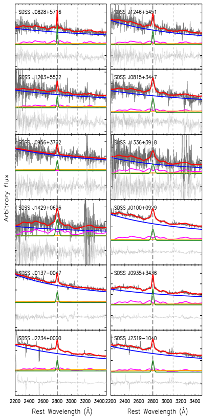
Figure 2.— Fully reduced GNIRS spectra of our targets in the spectral region around the Mg II emission after 3 pixel smoothing (gray solid line), where the best-fit results are overlaid. Total fit (red), power-law continuum (blue), Balmer-pseudo continuum (orange), Fe II (magenta), and Mg II (green) are shown respectively. The residual spectrum (thin gray solid line) is shown in the lower panel for each target.

III.2. H$\beta$ and AGN properties

We also measured AGN properties (i.e., $M_{\rm BH}$, luminosity, and Eddington ratio). The mass of SMBHs was calculated using the single-epoch method (Vestergaard, 2002; Wu et al., 2004; Vestergaard & Peterson, 2006; Park et al., 2012; Matsuoka et al., 2013; Karouzos et al., 2015) based on the dispersion of emission lines and continuum luminosity. Specifically, three emission lines have been often used, namely, H$\beta$ $\lambda$4861, Mg II, and C IV, combined with the continuum luminosity density at 5100, 2800, and 1350Å respectively. In this work, we used H$\beta$ with the continuum luminosity density at 5100Å for the high-z quasars since it is well calibrated compared to the other emission lines (e.g., Park et al., 2012). For low-redshift quasars, we used Mg II and the continuum luminosity density at 3000Å to measure the AGN properties since we have no H$\beta$ information.

For fitting the spectral region around the H$\beta$ emission, we took into account of a power-law continuum, [O III], and narrow- and broad- components of H$\beta$. No apparent signature of the Fe II multiplet and host galaxy stellar absorption lines are present in the rest-frame optical part of the spectra. Thus, we do not include the Fe II and stellar components in the fitting procedure. Note that it is a general trend that the Fe II multiplet emission in the rest-frame optical is weaker than that in the rest-frame UV (e.g., Tsuzuki et al., 2006).

We fitted each of the [O III]$\lambda\lambda$4959,5007 doublet with a double Gaussian model Similar to Mg II, the fit with the Gauss-Hermite series tends to be largely affected by noise and thus the Gauss-Hermite profile was not used for fitting the [O III] line. For the H$\beta$ emission, we adopted the line profile of [O III] as the H$\beta$ narrow component with a flux scaling, while we used a double Gaussian model to fit the broad H$\beta$ line. Note that the narrow component of the H$\beta$ to the [O III]  flux ratio is within the range of 5–40%, that is consistent with previous works (e.g., Park et al., 2012). Then we calculated $M_{\rm BH}$ using the velocity dispersion of the broad H$\beta$ broad line and the continuum luminosity density at 5100Å by adopting Equation 2 of Woo et al. (2015). Also, $M_{\rm BH}$ based on the velocity dispersion of Mg II and the continuum luminosity density at 3000Å was calculated using the equation given in Woo et al. (2018). The bolometric luminosity of AGNs was derived from the continuum luminosity density at 3000Å and 5100Å, by multiplying a bolometric correction factor of 5.15 (for 3000Å) and 9.26 (for 5100Å) given in Shen et al. (2008). The Eddington ratio was calculated by dividing the derived bolometric luminosity by the Eddington luminosity determined using $M_{\rm BH}$. The uncertainties of these AGN properties were estimated using Monte-Carlo simulations. The results are listed in Table 2.

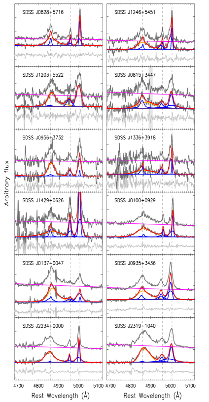
Figure 3.— Same as Figure 2 but for the spectral region around the H$\beta$ emission. Total fit (red), power-law continuum (magenta), and the [O III] and narrow H$\beta$ components (blue) are presented. Also, the broad component of H$\beta$ is shown in orange.

III.3. N V/C IV

As an another indicator of chemical properties of the BLR in quasars, we measured the N V/C IV flux ratio of our sample using the optical SDSS spectra. Since many UV emission lines are heavily blended (e.g., Ly$\alpha$$\lambda$1216 and N V), we conducted multi-component fitting analysis by adopting the same procedure as adopted by Shin et al. (2013). In the fitting, we divided broad emission lines into two groups based on the ionization potential of the corresponding ion (i.e., high- and low-ionization emission lines) assuming the same kinematics (the line shift and dispersion) for these emission lines in each group (see, e.g., McIntosh et al., 1999). We adopted a double Gaussian model for fitting the emission lines. Then, the N V/C IV flux ratio was calculated from the best fit model. Its uncertainties were estimated from the signal-to-noise ratio of the SDSS spectrum, and the derived flux ratio and its uncertainty are presented in Table 2.

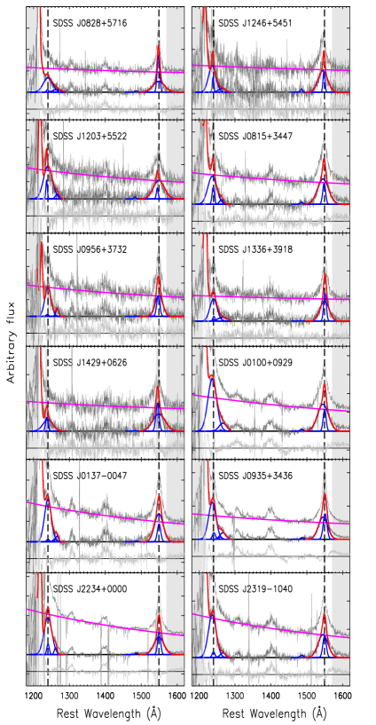
Figure 4.— SDSS spectra of our targets for the spectral region around the N V and C IV emission. Total fit (red), power-law continuum (magenta), and the N V and C IV components (blue) are shown respectively. The residual spectrum (thin gray solid line) is shown in the lower panel for each target.

Table 2Line flux ratios and AGN properties

Target	log FeII/MgII	log FeII/MgII	log FeII/MgII	log FeII/MgII	log NV/CIV	log $M_{\rm BH}/M_{\odot}$	log $L_{\rm Bol}$	log $L_{\rm Bol}/L_{\rm Edd}$
	(T06)	(VW01)	(mo_VW01)	(mo_VW011860)			(erg s-1)
(1)	(2)	(3)	(4)	(5)	(6)	(7)	(8)	(9)
SDSS J082854.44+571637.2	$0.79\pm 0.03$	$0.56\pm 0.03$	$0.60\pm 0.04$	$0.63\pm 0.04$	$-0.21\pm 0.10$	$9.08\pm 0.27$	$46.62\pm 0.00$	$-0.55\pm 0.28$
SDSS J124652.80+545140.6	$0.68\pm 0.06$	$0.42\pm 0.06$	$0.45\pm 0.06$	$0.46\pm 0.06$	$-0.04\pm 0.15$	$9.15\pm 0.22$	$46.65\pm 0.00$	$-0.59\pm 0.22$
SDSS J120308.69+552245.8	$0.66\pm 0.34$	$0.37\pm 0.36$	$0.40\pm 0.37$	$0.35\pm 0.42$	$0.15\pm 0.10$	$8.83\pm 0.22$	$46.62\pm 0.02$	$-0.30\pm 0.23$
SDSS J081528.12+344737.0	$0.47\pm 0.24$	$0.27\pm 0.20$	$0.28\pm 0.21$	$0.30\pm 0.20$	$-0.08\pm 0.06$	$9.15\pm 0.16$	$46.69\pm 0.01$	$-0.56\pm 0.17$
SDSS J095617.14+373224.7	$<0.45^{\ast}$	$<-0.20^{\ast}$	$<-0.19^{\ast}$	$<-0.33^{\ast}$	$-0.08\pm 0.09$	$8.39\pm 0.31$	$46.39\pm 0.01$	$-0.09\pm 0.31$
SDSS J133600.20+391826.2	$0.77\pm 0.23$	$0.46\pm 0.16$	$0.49\pm 0.17$	$0.46\pm 0.19$	$-0.17\pm 0.12$	$8.91\pm 0.31$	$46.20\pm 0.01$	$-0.81\pm 0.31$
SDSS J142903.86+062620.4	$0.69\pm 0.14$	$0.42\pm 0.13$	$0.44\pm 0.14$	$0.43\pm 0.14$	$-0.31\pm 0.16$	$9.06\pm 0.32$	$46.38\pm 0.02$	$-0.78\pm 0.34$
SDSS J010049.76+092936.1	$0.65\pm 0.02$	$0.42\pm 0.02$	$0.44\pm 0.02$	$0.43\pm 0.02$	$0.10\pm 0.03$	$9.55\pm 0.17$	$47.22\pm 0.00$	$-0.42\pm 0.17$
SDSS J013735.46-004723.4	$0.31\pm 0.06$	$0.04\pm 0.07$	$0.06\pm 0.07$	$0.05\pm 0.08$	$-0.01\pm 0.04$	$9.08\pm 0.05$	$46.97\pm 0.00$	$-0.21\pm 0.05$
SDSS J093514.41+343659.5	$0.66\pm 0.01$	$0.44\pm 0.01$	$0.47\pm 0.01$	$0.47\pm 0.01$	$-0.01\pm 0.03$	$9.23\pm 0.04$	$47.19\pm 0.00$	$-0.14\pm 0.05$
SDSS J223408.99+000001.6	$0.68\pm 0.01$	$0.43\pm 0.01$	$0.45\pm 0.01$	$0.46\pm 0.01$	$0.12\pm 0.01$	$9.42\pm 0.01$	$47.82\pm 0.00$	$0.29\pm 0.01$
SDSS J231934.77–104037.0	$0.63\pm 0.02$	$0.40\pm 0.01$	$0.42\pm 0.01$	$0.42\pm 0.02$	$0.07\pm 0.03$	$9.08\pm 0.09$	$47.39\pm 0.00$	$0.21\pm 0.09$

Note. — $\ast$: 2 sigma upper limit.

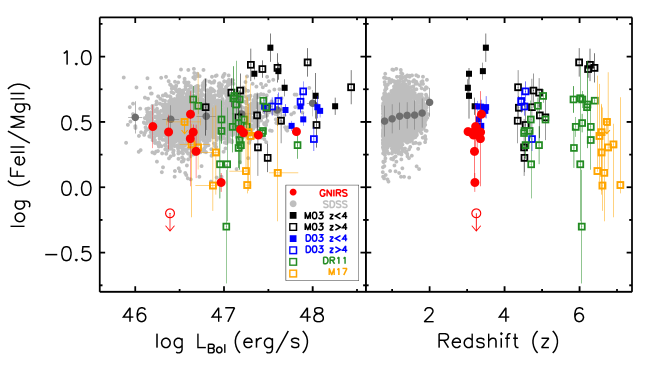
Figure 5.— Fe II/Mg II ratio as a function of AGN bolometric luminosity (left) and redshift (right). Our $z\sim 3$ sample (red) is compared to the samples from Maiolino et al. (2003, M03) (black), Dietrich et al. (2003, D03) (blue), De Rosa et al. (2011, DR11) (green), and Mazzucchelli et al. (2017, M17) (yellow). Our low-z SDSS sample is denoted with light-gray (each object) and dark-gray circles (binned data). Filled squares indicate the measurements for quasars at $z<4$, while open squares show the measurements for high-redshift ($>4$) quasars. One AGN with an upper limit of Fe II/MgII in our sample is denoted with an open red circle. Note that for comparing with the Fe II/Mg II ratio of the literature samples, we adopted the Fe II/Mg II ratio measurements based on the VW01 template (see Table 2).

IV. result

IV.1. Fe II/Mg II ratio

In Figure 5, we compare the Fe II/Mg II flux ratio of our quasar sample with the previous results from the literature (Maiolino et al., 2003; Dietrich et al., 2003; De Rosa et al., 2011; Mazzucchelli et al., 2017) as a function of the redshift and bolometric luminosity. We note that Maiolino et al. (2003) and Dietrich et al. (2003) provided only $L_{1450}$ and we converted it to bolometric luminosity using the bolometric correction factor of 4.2 (Runnoe et al., 2012). Here we present the Fe II/Mg II measurements based on the VW01 template in Figure 5 to be consistent with previous results (Maiolino et al., 2003; Dietrich et al., 2003; De Rosa et al., 2011; Mazzucchelli et al., 2017). Note that the Fe II/Mg II flux ratios based on VW01 and mo_VW01 (also mo_VW01_1860) are consistent within $\sim$0.025 dex ($\sim$ 6%) on average, and thus, this difference does not change any trend in Figure 5.

We find that, among our sample at $z\sim 3$, lower-luminosity quasars do not show lower Fe II/Mg II flux ratios than higher-luminosity quasars. In other words, the Fe II/Mg II flux ratio appears to be independent of the AGN luminosity for our quasars at $z\sim 3$ as they show similar values within the uncertainty except for two outliers (SDSS J0137–0047 and SDSS J0956+3732). In the case of the SDSS quasars at $z\lesssim 2$, while bolometric luminosity is similar to that of our sample, Fe II/Mg II flux ratio is similar to that of $z\sim 3$ quasars in our sample. We calculate the mean Fe II/Mg II flux ratio of the SDSS quasars in each luminosity/redshift bin and the uncertainties of them were taken from the standard deviation of the values in each bin. Even though the mean values of Fe II/Mg II show weak evolution as a function of redshift, they are consistent within the uncertainties. In contrast, our measurements of Fe II/Mg II flux ratio are significantly lower than those of Maiolino et al. (2003) at similar redshift ($z\sim 3$), indicating the effect of luminosity. We will discuss possible origins of this discrepancy in the next section.

We also find that there is no significant Fe II/Mg II evolution as a function of redshift. Even though there are systematic differences between each study, our result is consistent with previous works (e.g., De Rosa et al., 2011; Mazzucchelli et al., 2017). For assessing the statistical significance quantitatively, we performed Spearman’s lank-order statistical test for the relation between the Fe II/Mg II flux ratio and the redshift, and also between the Fe II/Mg II flux ratio and $L_{\rm Bol}$. The obtained correlation coefficients and Spearman’s lank-order probabilities for only high-z quasars (except for low-redshift SDSS quasars and SDSS J0956+3732) are 0.327 and 0.007 for $L_{\rm Bol}$, and 0.125 and 0.313 for the redshift. If we include low-z SDSS quasars, the coefficients become 0.166 and 3.87$\times 10^{-27}$ for $L_{\rm Bol}$, and 0.167 and 1.95 $\times 10^{-27}$ for the redshift. The results of Spearman’s lank-order statistical test infer a positive correlation between the Fe II/Mg II flux ratio and both redshift and luminosity, if quasars at all redshift ranges are considered, but this result is presumably mainly due to the objects with high-luminosity and high Fe II/MgII ratio from Maiolino et al. (2003). Since there is a large scatter of Fe II/Mg II flux ratio in each sample and in the total sample, it is difficult to confirm the correlation.

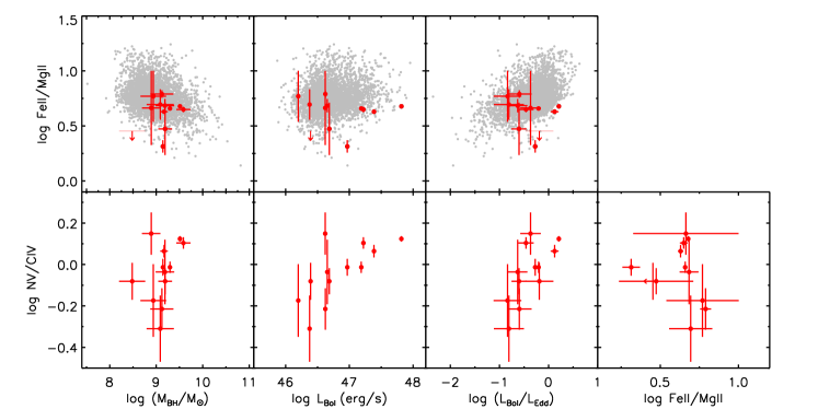
Figure 6.— Relation between two BLR emission-line flux ratios (Fe II/Mg II and N V/C IV in upper and lower panels respectively) and AGN properties (black hole mass, bolometric luminosity, and Eddington ratio, shown in left, middle, and right panels, respectively). Filled red and gray circles denote high-$z$ and low-$z$ samples of ours, respectively.

IV.2. The metallicity dependence on AGN properties

We investigate the dependency of the Fe II/Mg II (based on the T06 template) and N V/C IV flux ratios on the AGN properties, i.e., the black hole mass, bolometric luminosity, and Eddington ratio. In Figure 6, the relations between Fe II/Mg II and AGN properties of low-z quasars show similar trend with those in Dong et al. (2011) and Sameshima et al. (2017). In contrast, the Fe II/Mg II of our sample of 12 high-z quasars show no clear dependency on AGN properties, presumably due to the small sample size, while their flux ratios are consistent with those of low-z AGNs. Spearman’s correlation test confirms a strong correlation between Fe II/Mg II and AGN properties for the combined sample of low-redshift SDSS quasars and high-redshift quasars, while little correlation is found between AGN properties and Fe II/Mg II if we use only high-redshift quasars (see Table 3). In the case of the N V/C IV flux ratio, we find strong dependence on the AGN properties, i.e., luminosity, mass, and Eddington ratio (see, e.g., Matsuoka et al., 2011b). We also investigate the relation between Fe II/Mg II and N V/C IV, finding no clear correlation. As suggested for the relation between Fe II/Mg II and AGN properties in our sample, this non-correlation is presumably due to the limited sample size.

Table 3Results of Spearman’s Rank-order correlation test

	$M_{\rm BH}/M_{\odot}$	$L_{\rm Bol}/L_{\odot}$	$L_{\rm Bol}/L_{\rm Edd}$
(1)	(2)	(3)	(4)
Fe II/Mg II	$r_{s}$= –0.409	$r_{s}$= –0.582	$r_{s}$= –0.500
	$p$= 0.212	$p$= 0.060	$p$= 0.117
Fe II/Mg II w/ SDSS	$r_{s}$= –0.309	$r_{s}$= 0.189	$r_{s}$= 0.486
	$p$= 0.000	$p$= 0.000	$p$= 0.000
N V/C IV	$r_{s}$= 0.400	$r_{s}$= 0.670	$r_{s}$= 0.642
	$p$= 0.197	$p$= 0.017	$p$= 0.024

V. Discussion

V.1. No Fe II/Mg II evolution of BLR in quasars

As discussed in Section 1, it is expected that low-luminosity quasars at high-z may show signatures of variations in the chemical composition traced by the Fe II/Mg II flux ratio, compared to low-z quasars (Kawakatu et al., 2003; Juarez et al., 2009). However, the observed Fe II/Mg II ratio of low-luminosity quasars (log $L_{\rm bol}\sim 46.5$) at z$\sim 3$ is comparable to those of low-z quasars and those of high-luminosity quasars (log $L_{\rm bol}\sim 47.5$) at similar redshift. Also, the Fe II/Mg II ratios in high-$z$ quasars (regardless of the bolometric luminosity) are similar to those in low-$z$ quasars. This suggests that there is no significant redshift evolution in the Fe/Mg abundance ratio. Though the N V/C IV flux ratio in our high-$z$ quasar sample show a clear dependence on the bolometric luminosity, the dependence does not show any redshift evolution (see Nagao et al. 2006b; Matsuoka et al. 2011b). Therefore, we conclude that there is no chemical evolution including the Fe/Mg abundance ratio, in quasars for a wide redshift range, i.e., $0\lesssim z\lesssim 3$. In other words, observed quasars are already matured chemically, even for high-$z$ low-luminosity quasars.

There are two exceptions showing a low Fe II/Mg II flux ratio (SDSS J0137–0047 and SDSS J0956+3732), which may imply that they are in a chemically young phase. However, since one of the two quasars, SDSS J0137–0047, has relatively high luminosity ($L_{\rm bol}=47.0$ erg s^-1), it does not support the idea that low-luminosity quasars are in a chemically young phase. One possible interpretation for the no evolution of Fe II/Mg II flux ratio is that our targets are still too luminous to look at quasars in a chemically-young phase. Maiolino et al. (2008) showed that the metallicity evolution of massive galaxies ($M_{\ast}/M_{\odot}\sim\ 10^{11}$) is less prominent than that of low-mass galaxies $M_{\ast}/M_{\odot}<10^{10}$ for $0<z<3$. Since the black hole mass of our high-$z$ quasar sample is typically $\sim$10⁹ $M_{\odot}$ (Table 2), the mass of their host galaxies is inferred to be $\sim$10${}^{11-12}\ M_{\odot}$ by assuming the $M_{\rm BH}$-to-stellar mass ratio to be $0.001-0.01$ Thus, our results suggest that our targets are already chemically evolved with the previous type 1a SN activities. To search for chemically-young quasars, it is necessary to use lower-luminosity quasars, whose $M_{\rm BH}$ is expected to be on average lower.

V.2. Fe II/Mg II and AGN properties

In Figure 6, the Fe II/Mg II ratios of low-redshift quasars show negative (positive) correlation with black hole mass (Eddington ratio) as reported by Dong et al. (2011). Since galaxy mass correlates with the Mg/Fe abundance ratio (e.g., Thomas et al., 2005; Johansson et al., 2012; Conroy et al., 2014) as well as galaxy black hole mass (e.g., Magorrian et al., 1998; Ferrarese & Merritt, 2000; Gebhardt et al., 2000; Marconi & Hunt, 2003; Häring & Rix, 2004; Kormendy & Ho, 2013; Woo et al., 2013, 2015), the correlation between the Fe II/Mg II flux ratio and $M_{\rm BH}$ is naturally expected, if the Fe II/Mg II flux ratio is a good indicator of the Fe/Mg abundance ratio.

On the other hand, Dong et al. (2011) also reported that the Fe II/Mg II flux ratio shows a stronger dependency on the Eddington ratio than on the black hole mass, suggesting that the Fe II/Mg II flux ratio is more likely governed by the gas density of the BLR, rather than the Fe/Mg abundance ratio (see also Sameshima et al., 2017). Using the photoionization code, Cloudy (Ferland et al., 1998), several theoretical works also showed that the Fe II/Mg II flux ratio depends on various physical parameters such as the turbulence and the BLR gas density (e.g., Verner et al., 2003; Baldwin et al., 2004; Sameshima et al., 2017). To investigate the Fe II/Mg II correlation with Eddington ratio, Sameshima et al. (2017) hypothesized that gas density correlates with Eddington ratio and discussed the possibility of the BLR radius-Eddington ratio relation (Rees et al., 1989), while the origin of gas density-Eddington ratio relation has not been discussed. By proposing the correction for the gas density dependence, they discussed the intrinsic Fe/Mg abundance ratio. Note that using the correction method (Eq. 12 of Sameshima et al. 2017), we find only 0.02 dex difference in the Fe II/Mg II flux ratio for our high-z quasars.

While the 12 high-z quasars in our sample have similar AGN properties compare to the low-z quasars, we do not find clear relations with AGN properties, presumably due to the relatively large error of the Fe II/Mg II flux ratio and the small sample size. To better understand these relations for high-z quasars, a large spectroscopic sample is needed.

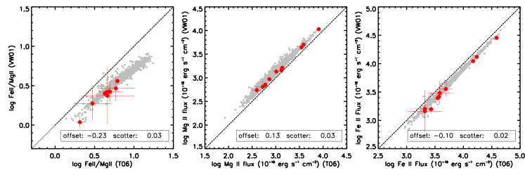
Figure 7.— Comparison of the measurement results by adopting different iron templates. Measurements with the T06 template and the VW01 template are shown in X-axis and Y-axis, respectively. Symbols are the same as in Figure 5.

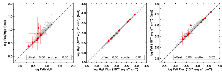
Figure 8.— Comparison of the measurement results with/without velocity constraint. Original measurements (with velocity constraint) presented in Table 2 are shown in X-axis, while the results without velocity constraint are shown in Y-axis. Symbols are the same as in Figure 5.

V.3. Systematic uncertainties of the Fe II/Mg II flux ratio

There is a discrepancy of the Fe II/Mg II flux ratio measurements among various studies as shown in Figure 5. For example, for one target in our sample SDSS J2234+0000, Maiolino et al. (2003) reported the Fe II/Mg II ratio as $5.77\pm 0.86$ while our measurement is $2.68\pm 0.06$, showing a factor of $\sim 2$ difference. Kurk et al. (2007) discussed several factors (e.g., the adopted iron template and the fitting method) that can severely affect the measurement of the Fe II/Mg II flux ratio, and found that such effects can result in a large difference in the measured Fe II/Mg II flux ratio by a factor of up to 2.

In order to investigate the systematic uncertainty in the Fe II/Mg II measurement, we conducted a couple of tests using the combined sample of 11 high-z quasars and $\sim$4000 low-z quasars. Note that we exclude SDSS J0956+3732 since its Fe II emission is not clearly detected in our observation (Section 4.1). First, we investigate the effect of the iron templates. As shown in Figure 1, the T06 template successfully recovers Fe II around the Mg II emission at 2800Å, which is not recovered by the VW01 template. We compare the Fe II/Mg II flux ratios along with the fluxes of Mg II, and Fe II, based on the templates of VW01 or T06 in Figure 7. We find that the T06 template provides an average higher Mg II flux (0.13 dex), lower Fe II flux (–0.10 dex), and higher Fe II/Mg II flux ratio (0.23 dex) than the VW01 template. This result indicates that the Fe II/Mg II flux ratio is underestimated when the VW01 template is adopted. If we use the modified VW01 template or the modified VW01 template with a fixed velocity dispersion, the Fe II/Mg II measurements are similar to those based on the VW01 template.

Second, we test the effect caused various fitting constraints, using the T06 template for the fitting. As shown in Figure 2, the Mg II emission is clearly present in the spectra while the excess of the Fe II emission above the continuum is not very significant in many cases. Therefore the measurement of the Fe II flux can be sensitive to the details of the fitting method. As described in Section 3.1, we used the full wavelength range of 2200–3090Å for the Fe II fitting with a constraint of the same velocity dispersion between the Mg II and Fe II emission. We test the Fe II/Mg II measurements with (1) no velocity dispersion constraint, (2) a narrower fitting range, and (3) a degraded spectral resolution as shown in Figures 7–9.

While Fe II and Mg II have similar ionization energies, using the same velocity dispersion between them may introduce a systematic uncertainty if the kinematics of the two ions are different. To examine this effect, we fit the spectra without tying the velocity dispersion between the Fe II and Mg II emission. We find that the Fe II/Mg II flux ratio with and without the velocity dispersion constraint are consistent to each other within 7%, implying that the constraint on the velocity dispersion produces no significant difference (see Figure 7).

For investigating the effect of the fitting range, we fit the spectra with a narrower fitting range of 2600–3050Å  instead of the range of 2200–3090Å (Figure 9). We find that the measurements from the two fitting ranges are consistent within 0.02 dex ($5\%$), with a scatter of 0.09 dex ($23\%$). The scatter is mainly due to the measurements of Fe II, rather than those of Mg II (see the middle and right panels in Figure 9). It is possible that the iron model is not perfect over the large fitting range. Thus, the measurements vary depending on the fitting range. Data quality is another cause of the scatter since there is an offset of 0.02 dex for the low-flux subsample (i.e., $<$ $10^{-14}\rm\ erg\ s^{-1}\ cm^{-2}$) while the higher-flux quasars show no offset (see the right panel in Figure 9).

We then test the effect of the spectral resolution. In Figure 5, we show that the measured Fe II/Mg II flux ratios by Maiolino et al. (2003) are systematically higher those in other studies (Dietrich et al. 2003 and this work). Maiolino et al. (2003) used the low spectral resolution, which was R$\sim$75 corresponding to 4000 km s^-1 in the velocity resolution. This low resolution may be a source of systematic uncertainties of the Fe II/ Mg II. To examine the spectral resolution effect, we smooth our spectra down to $R\sim 75$ and measure the Fe II/Mg II flux ratio in the smoothed spectra. The measured Fe II/Mg II ratios before and after the smoothing are compared in Figure 10, which shows a 0.09 dex scatter.

In summary, we find that adopting a proper iron template is the most important in measuring Fe II and Mg II fluxes. While the velocity dispersion constraint no significantly affect the Fe II and Mg II flux measurement, the fitting range and the spectral resolution introduces non-negligible uncertainties. For the investigation of the Fe II/Mg II flux ratio, a sufficiently large sample is necessary to overcome the systematic uncertainties and avoid the sample selection bias.

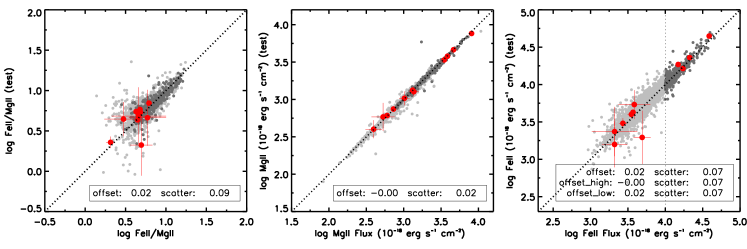
Figure 9.— Comparison of the measurement results by adopting two different fitting ranges. Our original measurements based on the fit for the range of 2200–3090Å and the measurements with a narrower fitting range of 2600–3050Å are shown in X- and Y- axes, respectively. Filled red and light gray circles denote high-$z$ and low-$z$ samples of ours, respectively. Dark gray circles denote low-$z$ sample with high flux ($\rm{\it F}_{Fe~{}{\sevenrm II}}$ ¿ $10^{-14}\ \rm erg\ s^{-1}\ cm^{-2}$).

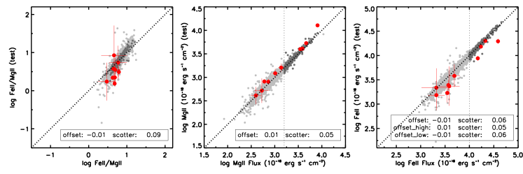
Figure 10.— Comparison between fittings with different resolution. Our original measurements and measurements from the spectrum with $R\sim$75 are shown in X- and Y- axes. Filled red and light gray circles denote high-$z$ and low-$z$ samples of ours, respectively. Dark gray circles shows low-$z$ sample with high flux ($\rm{\it F}_{Fe~{}{\sevenrm II}}$ ¿ $10^{-14}\ \rm\ erg\ s^{-1}\ cm^{-2}$ and $\rm{\it F}_{Mg~{}{\sevenrm II}}$ ¿ $10^{-14.8}\ \rm\ erg\ s^{-1}\ cm^{-2}$).

VI. Summary

We present the analysis of the Fe II/Mg II flux ratio measurements for a sample of quasars at z$\sim 3$, based on the NIR spectrum obtained with the Gemini/GNIRS. The sample with an order of magnitude lower luminosity than the quasars at similar redshift studied in the previous works, is selected to investigate the evolution of Fe II/Mg II at high redshift $z\sim$3–6, since the low-luminosity quasars may show a signature of chemically young status. We find that the low-luminosity quasars (log $L_{\rm bol}\sim 46.5$) show similar Fe II/Mg II ratios compared to those of high-luminosity quasars (log $L_{\rm bol}\sim 47.5$) at similar redshift, implying that even the low-luminosity quasars in our sample are already matured. To search for chemically young quasars with low Fe II/MgII ratios, quasars with much lower luminosity (i.e., log $L_{\rm bol}<46$) are necessary to study with upcoming extremely large telescopes. We find that the Fe II/Mg II flux ratio correlates with black hole mass and Eddington ratio, which is consistent with the previous results in the literature. By testing with various iron templates, fitting parameters, fitting range, we investigated systematic uncertainties, concluding that a consistent method for measuring the Fe II/Mg II flux ratio is required to compare with other works in investigating the evolution of the ratio.

References

- Abazajian et al. (2009) Abazajian, K. N., Adelman-McCarthy, J. K., Agüeros, M. A., et al. 2009, ApJS, 182, 543
- Ahn et al. (2012) Ahn, C. P., Alexandroff, R., Allende Prieto, C., et al. 2012, ApJS, 203, 21
- Alam et al. (2015) Alam, S., Albareti, F. D., Allende Prieto, C., et al. 2015, ApJS, 219, 12
- Amorín et al. (2014) Amorín, R., Grazian, A., Castellano, M., et al. 2014, ApJ, 788, L4
- Baldwin et al. (2004) Baldwin, J. A., Ferland, G. J., Korista, K. T., Hamann, F., & LaCluyzé, A. 2004, ApJ, 615, 610
- Barth et al. (2003) Barth, A. J., Martini, P., Nelson, C. H., & Ho, L. C. 2003, ApJ, 594, L95
- Conroy et al. (2014) Conroy, C., Graves, G. J., & van Dokkum, P. G. 2014, ApJ, 780, 33
- Cooke & Rodgers (2005) Cooke, A., & Rodgers, B. 2005, in Astronomical Society of the Pacific Conference Series, Vol. 347, Astronomical Data Analysis Software and Systems XIV, ed. P. Shopbell, M. Britton, & R. Ebert, 514
- De Rosa et al. (2011) De Rosa, G., Decarli, R., Walter, F., et al. 2011, ApJ, 739, 56
- De Rosa et al. (2014) De Rosa, G., Venemans, B. P., Decarli, R., et al. 2014, ApJ, 790, 145
- Dietrich et al. (2003) Dietrich, M., Hamann, F., Appenzeller, I., & Vestergaard, M. 2003, ApJ, 596, 817
- Dong et al. (2011) Dong, X.-B., Wang, J.-G., Ho, L. C., et al. 2011, ApJ, 736, 86
- Dors et al. (2014) Dors, O. L., Cardaci, M. V., Hägele, G. F., & Krabbe, Â. C. 2014, MNRAS, 443, 1291
- Elias et al. (2006) Elias, J. H., Joyce, R. R., Liang, M., et al. 2006, in Proc. SPIE, Vol. 6269, Society of Photo-Optical Instrumentation Engineers (SPIE) Conference Series, 62694C
- Ferland et al. (1998) Ferland, G. J., Korista, K. T., Verner, D. A., et al. 1998, PASP, 110, 761
- Ferrarese & Merritt (2000) Ferrarese, L., & Merritt, D. 2000, ApJ, 539, L9
- Gebhardt et al. (2000) Gebhardt, K., Bender, R., Bower, G., et al. 2000, ApJ, 539, L13
- Grandi (1982) Grandi, S. A. 1982, ApJ, 255, 25
- Hamann & Ferland (1992) Hamann, F., & Ferland, G. 1992, ApJ, 391, L53
- Hamann & Ferland (1993) —. 1993, ApJ, 418, 11
- Häring & Rix (2004) Häring, N., & Rix, H.-W. 2004, ApJ, 604, L89
- Iwamuro et al. (2004) Iwamuro, F., Kimura, M., Eto, S., et al. 2004, ApJ, 614, 69
- Jiang et al. (2007) Jiang, L., Fan, X., Vestergaard, M., et al. 2007, AJ, 134, 1150
- Johansson et al. (2012) Johansson, J., Thomas, D., & Maraston, C. 2012, MNRAS, 421, 1908
- Juarez et al. (2009) Juarez, Y., Maiolino, R., Mujica, R., et al. 2009, A&A, 494, L25
- Karouzos et al. (2015) Karouzos, M., Woo, J.-H., Matsuoka, K., et al. 2015, ApJ, 815, 128
- Kawakatu et al. (2003) Kawakatu, N., Umemura, M., & Mori, M. 2003, ApJ, 583, 85
- Kormendy & Ho (2013) Kormendy, J., & Ho, L. C. 2013, ARA&A, 51, 511
- Kurk et al. (2007) Kurk, J. D., Walter, F., Fan, X., et al. 2007, ApJ, 669, 32
- Lequeux et al. (1979) Lequeux, J., Peimbert, M., Rayo, J. F., Serrano, A., & Torres-Peimbert, S. 1979, A&A, 80, 155
- Magorrian et al. (1998) Magorrian, J., Tremaine, S., Richstone, D., et al. 1998, AJ, 115, 2285
- Maiolino et al. (2003) Maiolino, R., Juarez, Y., Mujica, R., Nagar, N. M., & Oliva, E. 2003, ApJ, 596, L155
- Maiolino et al. (2008) Maiolino, R., Nagao, T., Grazian, A., et al. 2008, A&A, 488, 463
- Mannucci et al. (2009) Mannucci, F., Cresci, G., Maiolino, R., et al. 2009, MNRAS, 398, 1915
- Marconi & Hunt (2003) Marconi, A., & Hunt, L. K. 2003, ApJ, 589, L21
- Matsuoka et al. (2009) Matsuoka, K., Nagao, T., Maiolino, R., Marconi, A., & Taniguchi, Y. 2009, A&A, 503, 721
- Matsuoka et al. (2011a) —. 2011a, A&A, 532, L10
- Matsuoka et al. (2011b) Matsuoka, K., Nagao, T., Marconi, A., Maiolino, R., & Taniguchi, Y. 2011b, A&A, 527, A100
- Matsuoka et al. (2013) Matsuoka, K., Silverman, J. D., Schramm, M., et al. 2013, ApJ, 771, 64
- Mazzucchelli et al. (2017) Mazzucchelli, C., Bañados, E., Venemans, B. P., et al. 2017, ApJ, 849, 91
- McGill et al. (2008) McGill, K. L., Woo, J.-H., Treu, T., & Malkan, M. A. 2008, ApJ, 673, 703
- McIntosh et al. (1999) McIntosh, D. H., Rix, H.-W., Rieke, M. J., & Foltz, C. B. 1999, ApJ, 517, L73
- McLure & Jarvis (2002) McLure, R. J., & Jarvis, M. J. 2002, MNRAS, 337, 109
- Nagao et al. (2012) Nagao, T., Maiolino, R., De Breuck, C., et al. 2012, A&A, 542, L34
- Nagao et al. (2006a) Nagao, T., Maiolino, R., & Marconi, A. 2006a, A&A, 447, 863
- Nagao et al. (2006b) Nagao, T., Marconi, A., & Maiolino, R. 2006b, A&A, 447, 157
- Onodera et al. (2016) Onodera, M., Carollo, C. M., Lilly, S., et al. 2016, ApJ, 822, 42
- Pâris et al. (2012) Pâris, I., Petitjean, P., Aubourg, É., et al. 2012, A&A, 548, A66
- Park et al. (2012) Park, D., Woo, J.-H., Treu, T., et al. 2012, ApJ, 747, 30
- Peng et al. (2006) Peng, C. Y., Impey, C. D., Rix, H.-W., et al. 2006, ApJ, 649, 616
- Rees et al. (1989) Rees, M. J., Netzer, H., & Ferland, G. J. 1989, ApJ, 347, 640
- Runnoe et al. (2012) Runnoe, J. C., Brotherton, M. S., & Shang, Z. 2012, MNRAS, 422, 478
- Sameshima et al. (2017) Sameshima, H., Yoshii, Y., & Kawara, K. 2017, ApJ, 834, 203
- Sanders et al. (2016) Sanders, R. L., Shapley, A. E., Kriek, M., et al. 2016, ApJ, 825, L23
- Schneider et al. (2010) Schneider, D. P., Richards, G. T., Hall, P. B., et al. 2010, AJ, 139, 2360
- Schramm et al. (2008) Schramm, M., Wisotzki, L., & Jahnke, K. 2008, A&A, 478, 311
- Schulze & Wisotzki (2014) Schulze, A., & Wisotzki, L. 2014, MNRAS, 438, 3422
- Shapley et al. (2017) Shapley, A. E., Sanders, R. L., Reddy, N. A., et al. 2017, ArXiv e-prints
- Shemmer & Netzer (2002) Shemmer, O., & Netzer, H. 2002, ApJ, 567, L19
- Shemmer et al. (2004) Shemmer, O., Netzer, H., Maiolino, R., et al. 2004, ApJ, 614, 547
- Shen et al. (2008) Shen, Y., Greene, J. E., Strauss, M. A., Richards, G. T., & Schneider, D. P. 2008, ApJ, 680, 169
- Shen et al. (2011) Shen, Y., Richards, G. T., Strauss, M. A., et al. 2011, ApJS, 194, 45
- Shin et al. (2017) Shin, J., Nagao, T., & Woo, J.-H. 2017, ApJ, 835, 24
- Shin et al. (2013) Shin, J., Woo, J.-H., Nagao, T., & Kim, S. C. 2013, ApJ, 763, 58
- Sommariva et al. (2012) Sommariva, V., Mannucci, F., Cresci, G., et al. 2012, A&A, 539, A136
- Thomas et al. (2005) Thomas, D., Maraston, C., Bender, R., & Mendes de Oliveira, C. 2005, ApJ, 621, 673
- Tremonti et al. (2004) Tremonti, C. A., Heckman, T. M., Kauffmann, G., et al. 2004, ApJ, 613, 898
- Troncoso et al. (2014) Troncoso, P., Maiolino, R., Sommariva, V., et al. 2014, A&A, 563, A58
- Tsuzuki et al. (2006) Tsuzuki, Y., Kawara, K., Yoshii, Y., et al. 2006, ApJ, 650, 57
- van der Marel & Franx (1993) van der Marel, R. P., & Franx, M. 1993, ApJ, 407, 525
- Verner et al. (2003) Verner, E., Bruhweiler, F., Verner, D., Johansson, S., & Gull, T. 2003, ApJ, 592, L59
- Vestergaard (2002) Vestergaard, M. 2002, ApJ, 571, 733
- Vestergaard & Peterson (2006) Vestergaard, M., & Peterson, B. M. 2006, ApJ, 641, 689
- Vestergaard & Wilkes (2001) Vestergaard, M., & Wilkes, B. J. 2001, ApJS, 134, 1
- Warner et al. (2003) Warner, C., Hamann, F., & Dietrich, M. 2003, ApJ, 596, 72
- Warner et al. (2004) —. 2004, ApJ, 608, 136
- Woo et al. (2018) Woo, J.-H., Le, H. A. N., Karouzos, M., et al. 2018, ApJ, 859, 138
- Woo et al. (2013) Woo, J.-H., Schulze, A., Park, D., et al. 2013, ApJ, 772, 49
- Woo et al. (2015) Woo, J.-H., Yoon, Y., Park, S., Park, D., & Kim, S. C. 2015, ApJ, 801, 38
- Wu et al. (2004) Wu, X.-B., Wang, R., Kong, M. Z., Liu, F. K., & Han, J. L. 2004, A&A, 424, 793
- Xu et al. (2018) Xu, F., Bian, F., Shen, Y., et al. 2018, MNRAS, 480, 345
- York et al. (2000) York, D. G., Adelman, J., Anderson, Jr., J. E., et al. 2000, AJ, 120, 1579