Output-Feedback Boundary Control of a Heat PDE Sandwiched Between Two ODEs

Abstract

We present designs for exponential stabilization of an ODE-heat PDE-ODE coupled system where the control actuation only acts in one ODE. The combination of PDE backstepping and ODE backstepping is employed in a state-feedback control law and in an observer that estimates PDE and two ODE states only using one PDE boundary measurement. Based on the state-feedback control law and the observer, the output-feedback control law is then proposed. The exponential stability of the closed-loop system and the boundedness and exponential convergence of the control law are proved via Lyapunov analysis. Finally, numerical simulations validate the effectiveness of this method for the “sandwiched” system.

I Introduction

Control of parabolic PDEs

Parabolic partial differential equations (PDEs) are predominately used in describing fluid, thermal, and chemical dynamics, including many applications of sea ice melting and freezing [28], continuous casting of steel [20] and lithium-ion batteries [15]. These therefore give rise to related important control and estimation problems, i.e., the boundary control and state observation of parabolic PDEs in [11, 14, 6, 19, 5, 7, 8, 18] and [2, 22, 23] respectively.

Control of parabolic PDE-ODE systems

In addition to the aforementioned works on parabolic PDEs, topics concerning parabolic PDE-ODE coupled systems are also popular, which have rich physical background such as coupled electromagnetic, coupled mechanical, and coupled chemical reactions [25]. Using the backstepping method, state-feedback and output-feedback control designs of a class of heat PDE-ODE couled systems were presented in [24, 26, 25]. The problem of state-observation is addressed for some parabolic PDE-ODE models in [1, 27]. The sliding model control was proposed to achieve boundary feedback stabilization of a heat PDE-ODE cascade system with external disturbances in [29].

Control of ODE-PDE-ODE systems

All aforementioned works consider actuation of PDE boundaries and ignore the dynamics of the actuator. However, sometimes the actuator dynamics may not be neglected, especially when dominant time constants of the actuator are closed to those of the plant. Considering the parabolic PDE-ODE coupled system with ODE actuator dynamics, it gives rise to a more challenging control/estimation problem of an ODE-PDE-ODE “sandwiched” system. Fewer attempts have been made on the boundary control of such an ODE-PDE-ODE system or PDE systems following ODE actuator dynamics where the controller acts. The boundary control of a viscous Burgers’ equation with an integration at the input, which is regarded as a first-order linear ODE in the input channel, was considered in [17]. Backstepping state-feedback control design for a transport PDE-ODE system where an integration at the input of the transport PDE was proposed in [9]. The control problem of an ODE with input delay and unmodeled bandwidth-limiting actuator dynamics, which is represented by an ODE-transport PDE-ODE system where the input ODE is first order, is successfully addressed in [13]. Stabilization of $2\times 2$ coupled linear first-order hyperbolic PDEs sandwiched around two ODEs was also achieved in [30].

In this paper, we use the combination of ODE backstepping and PDE backstepping methods to exponentially stabilize an ODE-heat PDE-ODE coupled system where the two ODEs are of arbitrary orders. An observer is designed to estimate all PDE and ODE states only using one PDE boundary value and then the observer-based output feedback control law is proposed.

Main contributions

• This is the first result of stabilizing such an ODE-parabolic PDE-ODE “sandwiched” system where the control action only acts in one ODE.

• Compared with our previous work [30] where a state-feedback control law was designed to stabilize the ODE-hyperbolic PDE-ODE system with the second-order input ODE and only a sketch of the design and analysis for an arbitrary-order input ODE was provided, in the present paper we extend the hyperbolic PDE to a parabolic PDE, where challenges appear because of the higher order spatial derivative and the inconformity between the orders of time and spatial derivatives. In addition, we design an observer to estimate all the states of the ODE-PDE-ODE system only using one PDE boundary value, and an output-feedback control law is proposed. Moreover, more detailed control design and stability analysis of the system where arbitrary-order ODEs sandwich around the PDE are presented.

• Compared with the previous results about stabilizing ODE-transport PDE-ODE systems where both ODEs are first order [9, 13, 4], in addition to replacing the transport PDE by a heat PDE, we achieve a more challenging and general result where the orders of both ODEs sandwiching the PDE are arbitrary.

Organization

The rest of the paper is organized as follows. The concerned model is presented in Section II. The state-feedback control design combining the PDE backstepping and ODE backstepping is shown in Section III. The observer design and the output-feedback control law with stability analysis of the closed-loop system are proposed in Section IV. The simulation results are provided in Section V. The conclusion and future work are presented in Section VI.

Throughout this paper, the partial derivatives and total derivatives are denoted as:

$${f_{x}}(x,t)= \frac{{\partial f}}{{\partial x}},~{}~{}\quad{f_{t}}(x,t)=\frac{{\partial f}}{{\partial t}},$$

$$\partial_{x}^{m}f(x,t) =\frac{{\partial^{m}f}}{{\partial x^{m}}},~{}~{}\partial_{t}^{m}f(x,t)=\frac{{\partial^{m}f}}{{\partial t^{m}}},$$

$$f^{\prime}(x)= \frac{{df}}{{dx}},\quad\dot{f}(t)=\frac{{df}}{{dt}},$$

$$d_{x}^{m}f(x) =\frac{{d^{m}f}}{{dx^{m}}},~{}~{}d_{t}^{m}f(t)=\frac{{d^{m}f}}{{dt^{m}}}.$$

II Problem statement

We consider the following system where two ODEs sandwich around a heat PDE as,

$$\dot{X}(t) =AX(t)+B{u_{x}}(0,t),$$ (1)

$${u_{t}}(x,t) =q{u_{xx}}(x,t),$$ (2)

$$u(0,t) ={C_{X}}X(t),$$ (3)

$$u(1,t) ={C_{z}}Z(t),$$ (4)

$$\dot{Z}(t) ={A_{z}}Z(t)+{B_{z}}U(t),$$ (5)

$\forall(x,t)\in[0,1]\times[0,\infty)$, where $X(t)\in\mathbb{R}^{n\times 1}$, $Z(t)\in\mathbb{R}^{m\times 1}$ are ODE states, $n,m\in N^{*}$, $N^{*}$ denoting positive integers. $u(x,t)\in R$ are states of the PDE. $\emph{A}\in\mathbb{R}^{n\times n}$, $\emph{B}\in\mathbb{R}^{n\times 1}$ satisfy that the pair $[A,B]$ is controllable. ${C_{X}}\in\mathbb{R}^{1\times n}$ and $q\in R$ are arbitrary. $A_{z}\in\mathbb{R}^{m\times m}$ is

$${A_{z}}=\left[{\begin{array}[]{*{20}{c}}0&1&0&0&\cdots&0\\ 0&0&1&0&\cdots&0\\ {}\hfil&{}\hfil&\vdots&{}\hfil&{}\hfil&{}\hfil\\ 0&0&0&0&\cdots&1\\ {{\bar{a}_{1}}}&{{\bar{a}_{2}}}&{{\bar{a}_{3}}}&\cdots&{{\bar{a}_{m-1}}}&{{\bar{a}_{m}}}\end{array}}\right]_{m\times m},$$ (11)

where $\bar{a}_{1},\cdots,\bar{a}_{m}$ are arbitrary constants. $B_{z}=[0,0,\cdots,1]^{T}\in\mathbb{R}^{m\times 1}$, $C_{z}=[1,0,\cdots,0]\in\mathbb{R}^{1\times m}$. Note that $(A_{z},B_{z})$ and $(A_{z},C_{z})$ are in the controllability normal form and observability normal form respectively. $U(t)$ is the control input to be designed.

The control objective is to exponentially stabilize all ODE states $Z(t),X(t)$ and PDE states $u(x,t)$ by designing a control input $U(t)$ in one ODE, and control input itself should be guaranteed exponentially convergent as well.

The control design in this paper can be applied in the Stefan problem describing the melting or solidification mechanism with liquid-solid dynamics [16], i.e., heat PDE-ODE , driven by a thermal actuator described by an ODE at the boundary of the liquid phase.

III State-Feedback Design

In this section, we combine the PDE backstepping (Section III-A) and the ODE backstepping (Section III-B) to design a state-feedback control law. Exponential stability of the state-feedback closed-loop system is proved in Section III-C. The boundedness and exponential convergence of the state-feedback control law is proved in Section III-D.

III-A Backstepping for PDE-ODE

We would like to use the infinite-dimensional backstepping transformations [12]:

$$w(x,t)=u(x,t)-\int_{0}^{x}{{\phi}}(x,y)u(y,t)dy-{\Phi}(x)X(t),$$ (12)

with the inverse transformation as

$$u(x,t)=w(x,t)-\int_{0}^{x}{{\psi}}(x,y)w(y,t)dy-{\Gamma}(x)X(t),$$ (13)

to convert the original system (1)-(3) to

$$\dot{X}(t) =(A+BK)X(t)+B{w_{x}}(0,t),$$ (14)

$${w_{t}}(x,t) =q{w_{xx}}(x,t),$$ (15)

$$w(0,t) =0,$$ (16)

where the right boundary condition $w(1,t)$ will be given later. $A+BK$ is Hurwitz by choosing the control parameter $K$ since $(A,B)$ is assumed controllable.

Mapping the original system (1)-(3) and the system (14)-(16) via the transformations (12)-(13), the explicit solutions of kernels in (12)-(13) can be obtained as

$${\phi}(x,y) =\left[C_{X},K-C_{X}BC_{X}\right]e^{D(x-y)}\left[\begin{array}[]{c}I\\ 0\end{array}\right]B,$$ (19)

$$\Phi(x) =\left[C_{X},K-C_{X}BC_{X}\right]e^{D(x-y)}\left[\begin{array}[]{c}I\\ 0\end{array}\right],$$ (22)

$$\psi(x,y) =\left[C_{X},K\right]e^{E(x-y)}\left[\begin{array}[]{c}I\\ 0\end{array}\right]B,$$ (25)

$$\Gamma(x) =\left[C_{X},K\right]e^{E(x-y)}\left[\begin{array}[]{c}I\\ 0\end{array}\right],$$ (28)

$0\leq y\leq x\leq 1$, where the matrix $I$ denotes the identity matrix of the appropriate dimension and $D,E$ are

$$D=\left(\begin{array}[]{cc}0&A\\ I&-BC_{X}\\ \end{array}\right),~{}~{}E=\left(\begin{array}[]{cc}0&A+BK\\ I&0\\ \end{array}\right),$$ (33)

which ensures the invertibility and boundedness of the backstepping transformation (12)-(13). The detailed calculations of the kernels are shown in [25]. Note that dealing with the right boundary condition in the following steps will not affect determination of the kernels in (12)-(13).

Let us now calculate the right boundary condition $w(1,t)$ of (14)-(16). The right boundary condition $w(1,t)$ can be obtained by taking the $m$-order time derivative of the transformation (12) at $x=1$, inserting the original right boundary condition and the inverse transformation (13).

Considering (4)-(5) with (11), the right boundary condition of the original system can be written as

$$\partial_{t}^{m}u(1,t) =\bar{a}_{1}u(1,t)+\sum_{k=1}^{m-1}\bar{a}_{k+1}\partial_{t}^{k}u(1,t)+U(t)$$

$$=\bar{a}_{1}u(1,t)+\sum_{k=1}^{m-1}\bar{a}_{k+1}q^{k}\partial_{x}^{2k}u(1,t)+U(t).$$ (34)

Taking the $m$ times derivative in $t$ of (12) at $x=1$, we have

$$\partial_{t}^{m}w(1,t)=\partial_{t}^{m}u(1,t)-{q^{m}}\int_{0}^{1}{\partial_{y}^{2m}\phi(1,y)u(y,t)}dy$$

$$+q^{m}\sum\limits_{i=1}^{2m}{}{(-1)^{i}}\partial_{y}^{i-1}\phi(1,1)\partial_{x}^{2m-i}u(1,t)$$

$$-\Phi(1){A^{m}}X(t)-\bigg{(}q^{m}\sum\limits_{i=1}^{2m}{}{(-1)^{i}}\partial_{y}^{i-1}\phi(1,0)\partial_{x}^{2m-i}$$

$$+\Phi(1)\sum\limits_{i=1}^{m}{}{A^{i-1}}B{q^{m-i}}\partial_{x}^{2(m-i)+1}\bigg{)}u(0,t),$$ (35)

for $m\in N^{*}$, where

$$\partial_{x}^{k}u(1,t)\triangleq\partial_{x}^{k}u(x,t)|_{x=1},~{}\partial_{x}^{k}u(0,t)\triangleq\partial_{x}^{k}u(x,t)|_{x=0}.$$

Insert (34) into (35) to replace $\partial_{t}^{m}u(1,t)$. Then rewrite $u$ in (35) as $w$ via the inverse transformation (13), where the $k$-order derivative of the inverse transformation (13) in $x$ would be used:

$$\partial_{x}^{k}u(x,t) =\partial_{x}^{k}\bigg{(}w(x,t)-\int_{0}^{x}{{\psi}}(x,y)w(y,t)dy-{\Gamma}(x)X(t)\bigg{)}$$

$$=\partial_{x}^{k}w(x,t)-\partial_{x}^{k}\bigg{(}\int_{0}^{x}{{\psi}}(x,y)w(y,t)dy\bigg{)}$$

$$\quad-d_{x}^{k}{\Gamma}(x)X(t)$$

$$=\partial_{x}^{k}w(x,t)-\int_{0}^{x}{\partial_{x}^{k}{\psi}(x,y)w(y,t)dy}$$

$$\quad-\sum\limits_{j=0}^{k-1}{}{\chi_{k\_j}}(x)\partial_{x}^{k-j-1}w(x,t)-d_{x}^{k}{\Gamma}(x)X(t)$$ (36)

for $k\in N^{*}$, where ${\chi_{k\_j}}(x)$ denoting the sum of $j$-order derivatives of $\psi(x,x)$ with respect to $x$, results from calculating $\partial_{x}^{k}(\int_{0}^{x}{{\psi}}(x,y)w(y,t)dy)$, as following

$${\chi_{k\_j}}(x)=\sum_{i=0}^{j}\bar{\eta}_{k\_j\_i}\partial_{x}^{i}\partial_{y}^{j-i}\psi(x,y)|_{(x,y)=(x,x)},$$ (37)

where constant coefficients $\bar{\eta}_{k\_j\_i}$ can be easily determined by calculating $\partial_{x}^{k}(\int_{0}^{x}{{\psi}}(x,y)w(y,t)dy)$ under some specific $k$ according to the order of the plant.

Through plugging (13), (36) into (35) where $\partial_{t}^{m}u(1,t)$ has been replaced by (34), the right boundary condition of the system-$w$ is obtained as:

$$\quad\partial_{t}^{m}w(1,t)$$

$$={{\bar{a}}_{1}}w(1,t)-{{\bar{a}}_{1}}\int_{0}^{1}{{\psi}(1,y)w(y,t)dy-{{\bar{a}}_{1}}{\Gamma}(1)X(t)}$$

$$\quad+\sum\limits_{k=1}^{m-1}{{{\bar{a}}_{k+1}}}{q^{k}}\bigg{(}\partial_{x}^{2k}w(1,t)-\int_{0}^{1}{\partial_{x}^{2k}}{\psi}(1,y)w(y,t)dy$$

$$\quad-\sum\limits_{j=0}^{2k-1}{{\chi_{2k\_j}}}(1)\partial_{x}^{2k-j-1}w(1,t)-d_{x}^{2k}{\Gamma}(1)X(t)\bigg{)}$$

$$\quad-{q^{m}}\int_{0}^{1}\partial_{y}^{2m}\phi(1,y)\bigg{(}w(y,t)-\int_{0}^{y}{\psi}(y,z)w(z,t)dz$$

$$\quad-{\Gamma}(y)X(t)\bigg{)}dy+{q^{m}}\sum\limits_{i=1}^{2m}{(-1)^{i}}\partial_{y}^{i-1}\phi(1,1)$$

$$\quad\times\bigg{(}\partial_{x}^{2m-i}w(1,t)-\int_{0}^{1}{\partial_{x}^{2m-i}}{\psi}(1,y)w(y,t)dy$$

$$\quad-\sum\limits_{j=0}^{2m-i-1}{{\chi_{2m-i\_j}}}(1)\partial_{x}^{2m-i-j-1}w(1,t)$$

$$\quad-d_{x}^{2m-i}{\Gamma}(1)X(t)\bigg{)}-\Phi(1){A^{m}}X(t)$$

$$\quad-{q^{m}}\sum\limits_{i=1}^{2m}{(-1)^{i}}\partial_{y}^{i-1}\phi(1,0)\bigg{(}\partial_{x}^{2m-i}w(0,t)$$

$$\quad-\sum\limits_{j=0}^{2m-i-1}{{\chi_{2m-i\_j}}}(0)\partial_{x}^{2m-i-j-1}w(0,t)$$

$$\quad-d_{x}^{2m-i}{\Gamma}(0)X(t)\bigg{)}+\Phi(1)\sum\limits_{i=1}^{m}{}{A^{i-1}}B{q^{m-i}}\bigg{(}\partial_{x}^{2(m-i)+1}w(0,t)$$

$$\quad-\sum\limits_{j=0}^{2(m-i)+1-1}{{\chi_{2(m-i)+1\_j}}}(0)\partial_{x}^{2(m-i)+1-j-1}w(0,t)$$

$$\quad-d_{x}^{2(m-i)+1}{\Gamma}(0)X(t)\bigg{)}+U(t)$$

$$=\bigg{[}{{\bar{a}}_{1}}+\sum\limits_{k=1}^{m-1}{{{\bar{a}}_{k+1}}}{q^{k}}\partial_{x}^{2k}-\sum\limits_{k=1}^{m-1}{{{\bar{a}}_{k+1}}}{q^{k}}\sum\limits_{j=0}^{2k-1}{{\chi_{2k\_j}}}(1)\partial_{x}^{2k-j-1}$$

$$\quad+{q^{m}}\sum\limits_{i=1}^{2m}{}{(-1)^{i}}\partial_{y}^{i-1}\phi(1,1)\partial_{x}^{2m-i}$$

$$\quad-{q^{m}}\sum\limits_{i=1}^{2m}{}{(-1)^{i}}\partial_{y}^{i-1}\phi(1,1)\sum\limits_{j=0}^{2m-i-1}{{\chi_{2m-i\_j}}}(x)\partial_{x}^{2m-i-j-1}\bigg{]}w(1,t)$$

$$\quad+\bigg{[}-{q^{m}}\sum\limits_{i=1}^{2m}{(-1)^{i}}\partial_{y}^{i-1}\phi(1,0)\partial_{x}^{2m-i}$$

$$\quad+{q^{m}}\sum\limits_{i=1}^{2m}{}{(-1)^{i}}\partial_{y}^{i-1}\phi(1,0)\sum\limits_{j=0}^{2m-i-1}{{\chi_{2m-i\_j}}}(0)\partial_{x}^{2m-i-j-1}$$

$$\quad+\Phi(1)\sum\limits_{i=1}^{m}{A^{i-1}}B{q^{m-i}}\partial_{x}^{2(m-i)+1}-\Phi(1)\sum\limits_{i=1}^{m}{A^{i-1}}B{q^{m-i}}$$

$$\quad\quad\times\sum\limits_{j=0}^{2(m-i)+1-1}{{\chi_{2(m-i)+1\_j}}}(0)\partial_{x}^{2(m-i)+1-j-1}\bigg{]}w(0,t)$$

$$\quad-\int_{0}^{1}{\bigg{[}{q^{m}}\sum\limits_{i=1}^{2m}{}{{(-1)}^{i}}\partial_{y}^{i-1}\phi(1,1)\partial_{x}^{2m-i}}{\psi}(1,y)+{{\bar{a}}_{1}}{\psi}(1,y)$$

$$\quad+\sum\limits_{k=1}^{m-1}{{{\bar{a}}_{k+1}}}{q^{k}}\partial_{x}^{2k}{\psi}(1,y)+{q^{m}}\partial_{y}^{2m}\phi(1,y)$$

$$\quad-{q^{m}}\int_{y}^{1}{\partial_{y}^{2m}\phi(1,z){\psi}(z,y)dz}\bigg{]}w(y,t)dy$$

$$\quad+\bigg{[}{q^{m}}\sum\limits_{i=1}^{2m}{}{(-1)^{i}}\partial_{y}^{i-1}\phi(1,0)d_{x}^{2m-i}{\Gamma}(0)-\Phi(1){A^{m}}$$

$$\quad-\Phi(1)\sum\limits_{i=1}^{m}{}{A^{i-1}}B{q^{m-i}}d_{x}^{2(m-i)+1}{\Gamma}(0)$$

$$\quad-{q^{m}}\sum\limits_{i=1}^{2m}{}{(-1)^{i}}\partial_{y}^{i-1}\phi(1,1)d_{x}^{2m-i}{\Gamma}(1)$$

$$\quad-\sum\limits_{k=1}^{m-1}{{{\bar{a}}_{k+1}}}{q^{k}}d_{x}^{2k}{\Gamma}(1)-{{\bar{a}}_{1}}{\Gamma}(1)$$

$$\quad+{q^{m}}\int_{0}^{1}{\partial_{y}^{2m}\phi(1,y){\Gamma}(y)}dy\bigg{]}X(t)+U(t),$$ (38)

where some typical operators are

$$\partial_{x}^{k}w(1,t)\triangleq\partial_{x}^{k}w(x,t)|_{x=1},~{}\partial_{x}^{k}w(0,t)\triangleq\partial_{x}^{k}w(x,t)|_{x=0},$$

$$\partial_{y}^{k}\phi(1,1)\triangleq\partial_{y}^{k}\phi(x,y)|_{(x,y)=(1,1)},~{}d_{x}^{k}\Gamma(0)\triangleq d_{x}^{k}\Gamma(x)|_{x=0}.$$

(38) is a $m$ order ODE system-$w(1,t)$ with a number of PDE state perturbation terms. For clarity, (38) can be written as

$$\partial_{t}^{m}w(1,t) =\mathcal{B}w(1,t)+\mathcal{C}w(0,t)$$

$$\quad-\int_{0}^{1}\mathcal{D}(y)w(y,t)dy+\mathcal{E}X(t)+U(t).$$ (39)

Note that (39) is the right boundary condition of the system (14)-(16). $\mathcal{B},\mathcal{C},\mathcal{D},\mathcal{E}$ in (39) correspond to the parts including derivative operators in the square brackets before $w(1,t)$, $w(0,t)$, $w(y,t)$, $X(t)$ in (38). $\mathcal{D}(y)$ is a function of $y$ and $\mathcal{E}$ is a constant vector. Note that

$$\mathcal{B}w(1,t)\triangleq(\mathcal{B}w(x,t))|_{x=1},~{}~{}\mathcal{C}w(0,t)\triangleq(\mathcal{C}w(x,t))|_{x=0}.$$

Theorem 1.

Considering the system (1)-(11) and the backstepping transformation (12)-(13), (38) holds for $m\in N^{*}$ which is the order of the ODE (5).

Proof.

According to the derivation of (38), i.e., (35)-(38), we know (38) is obtained by inserting the plant dynamics (34) and (36) into (35) straightforwardly, so the correctness of (38) depends on that of (36) and (35). Next, we prove the correctness of (36) and (35) by induction. In detail, in order to prove the statement that (35) and (36) hold for arbitrary positive integers $m,k$, we first prove (35) and (36) are true in the initial cases $m=1,2$, $k=1,2$, and then assume they are true for $m={\bar{n}}$, $k={\bar{n}}$ and show they hold for $m={\bar{n}}+1$, $k={\bar{n}}+1$ respectively where ${\bar{n}}$ is a positive integer.

Proof of correctness of (35) by induction:

a). Checking the initial cases $m=1,2$. It is easily to see that (35) is true when $m=1$. Here we show the checking for the case $m=2$.

Taking twice time derivatives of (12), we have

$${w_{tt}}(1,t)= {u_{tt}}(1,t)-{q^{2}}\phi(1,1){u_{xxx}}(1,t)+{q^{2}}\phi(1,0){u_{xxx}}(0,t)$$

$$+{q^{2}}{\phi_{y}}(1,1){u_{xx}}(1,t)-{q^{2}}{\phi_{y}}(1,0){u_{xx}}(0,t)$$

$$-{q^{2}}{\phi_{yy}}(1,1){u_{x}}(1,t)+{q^{2}}{\phi_{yy}}(1,0){u_{x}}(0,t)$$

$$+{q^{2}}{\phi_{yyy}}(1,1)u(1,t)-{q^{2}}{\phi_{yyy}}(1,0)u(0,t)$$

$$-{q^{2}}\int_{0}^{1}{{\phi_{yyyy}}(1,y)u(y,t)}dy-\Phi(1){A^{2}}X(t)$$

$$-\Phi(1)AB{u_{x}}(0,t)-\Phi(1)B{u_{xt}}(0,t).$$ (40)

Setting $m=2$ in (35), we obtain

$$\partial_{t}^{2}w(1,t)=\partial_{t}^{2}u(1,t)-{q^{2}}\int_{0}^{1}{\partial_{y}^{4}\phi(1,y)u(y,t)}dy$$

$$+q^{2}\sum\limits_{i=1}^{4}{}{(-1)^{i}}\partial_{y}^{i-1}\phi(1,1)\partial_{x}^{4-i}u(1,t)$$

$$-\Phi(1){A^{2}}X(t)-q^{2}\sum\limits_{i=1}^{4}{}{(-1)^{i}}\partial_{y}^{i-1}\phi(1,0)\partial_{x}^{4-i}u(0,t)$$

$$+\Phi(1)\sum\limits_{i=1}^{2}{}{A^{i-1}}B{q^{2-i}}\partial_{x}^{2(2-i)}u_{x}(0,t),$$ (41)

where ${q^{2-i}}\partial_{x}^{2(2-i)}u_{x}(0,t)=\partial_{t}^{(2-i)}u_{x}(0,t)$ is used. It can be seen that (41) is equal to (40), so (35) is true when $m=2$.

b). Under the induction hypothesis that (35) holds for $m={\bar{n}}$, show it also holds for $m={\bar{n}}+1$.

Then we can assume (35) is true for $m={\bar{n}}$ which is a positive integer and next prove (35) also holds for $m={\bar{n}}+1$.

Taking the time derivative of (35) with setting $m={\bar{n}}$ we have

$$\quad\partial_{t}^{{\bar{n}}+1}w(1,t)$$

$$=\partial_{t}^{{\bar{n}}+1}u(1,t)-{q^{{\bar{n}}}}\int_{0}^{1}{\partial_{y}^{2{\bar{n}}}\phi(1,y){u_{t}}(y,t)}dy$$

$$\quad-\Phi(1){A^{{\bar{n}}}}\dot{X}(t)+\sum\limits_{i=1}^{2{\bar{n}}}{{q^{{\bar{n}}}}}{(-1)^{i}}\partial_{y}^{i-1}\phi(1,1)\partial_{xt}^{2{\bar{n}}-i}u(1,t)$$

$$\quad-\bigg{[}\sum\limits_{i=1}^{2{\bar{n}}}{{q^{{\bar{n}}}}}{(-1)^{i}}\partial_{y}^{i-1}\phi(1,0)\partial_{x}^{2{\bar{n}}-i}$$

$$\quad+\Phi(1)\sum\limits_{i=1}^{{\bar{n}}}{}{A^{i-1}}B{q^{{\bar{n}}-i}}\partial_{x}^{2({\bar{n}}-i)+1}\bigg{]}{u_{t}}(0,t)$$

$$=\partial_{t}^{{\bar{n}}+1}u(1,t)-{q^{{\bar{n}}+1}}\int_{0}^{1}{\partial_{y}^{2{\bar{n}}}\phi(1,y){u_{xx}}(y,t)}dy$$

$$\quad-\Phi(1){A^{{\bar{n}}+1}}X(t)-\Phi(1){A^{{\bar{n}}}}B{u_{x}}(0,t)$$

$$\quad+\sum\limits_{i=1}^{2{\bar{n}}}{{q^{{\bar{n}}+1}}}{(-1)^{i}}\partial_{y}^{i-1}\phi(1,1)\partial_{x}^{2({\bar{n}}+1)-i}u(1,t)$$

$$\quad-\bigg{[}\sum\limits_{i=1}^{2{\bar{n}}}{{q^{{\bar{n}}}}}{(-1)^{i}}\partial_{y}^{i-1}\phi(1,0)\partial_{x}^{2{\bar{n}}-i}$$

$$\quad+\Phi(1)\sum\limits_{i=1}^{{\bar{n}}}{}{A^{i-1}}B{q^{{\bar{n}}-i}}\partial_{x}^{2({\bar{n}}-i)+1}\bigg{]}q{u_{xx}}(0,t)$$

$$=\partial_{t}^{{\bar{n}}+1}u(1,t)-{q^{{\bar{n}}+1}}\partial_{y}^{2{\bar{n}}}\phi(1,1){u_{x}}(1,t)$$

$$\quad+{q^{{\bar{n}}+1}}\partial_{y}^{2{\bar{n}}}\phi(1,0){u_{x}}(0,t)$$

$$\quad+{q^{{\bar{n}}+1}}\partial_{y}^{2{\bar{n}}+1}\phi(1,1)u(1,t)-{q^{{\bar{n}}+1}}\partial_{y}^{2{\bar{n}}+1}\phi(1,0)u(0,t)$$

$$\quad-{q^{{\bar{n}}+1}}\int_{0}^{1}{\partial_{y}^{2({\bar{n}}+1)}\phi(1,y)u(y,t)}dy$$

$$\quad-\Phi(1){A^{{\bar{n}}+1}}X(t)-\Phi(1){A^{{\bar{n}}}}B{u_{x}}(0,t)$$

$$\quad+\sum\limits_{i=1}^{2{\bar{n}}}{{q^{{\bar{n}}+1}}}{(-1)^{i}}\partial_{y}^{i-1}\phi(1,1)\partial_{x}^{2({\bar{n}}+1)-i}u(1,t)$$

$$\quad-\bigg{[}\sum\limits_{i=1}^{2{\bar{n}}}{{q^{{\bar{n}}}}}{(-1)^{i}}\partial_{y}^{i-1}\phi(1,0)\partial_{x}^{2{\bar{n}}-i}$$

$$\quad+\Phi(1)\sum\limits_{i=1}^{{\bar{n}}}{}{A^{i-1}}B{q^{{\bar{n}}-i}}\partial_{x}^{2({\bar{n}}-i)+1}\bigg{]}q{u_{xx}}(0,t)$$

$$=\partial_{t}^{{\bar{n}}+1}u(1,t)+{q^{{\bar{n}}+1}}\partial_{y}^{2{\bar{n}}}\phi(1,0){u_{x}}(0,t)$$

$$\quad-{q^{{\bar{n}}+1}}\partial_{y}^{2{\bar{n}}+1}\phi(1,0)u(0,t)$$

$$\quad-{q^{{\bar{n}}+1}}\int_{0}^{1}{\partial_{y}^{2({\bar{n}}+1)}\phi(1,y)u(y,t)}dy$$

$$\quad-\Phi(1){A^{{\bar{n}}+1}}X(t)-\Phi(1){A^{{\bar{n}}}}B{u_{x}}(0,t)$$

$$\quad+\sum\limits_{i=1}^{2({\bar{n}}+1)}{{q^{{\bar{n}}+1}}}{(-1)^{i}}\partial_{y}^{i-1}\phi(1,1)\partial_{x}^{2({\bar{n}}+1)-i}u(1,t)$$

$$\quad-\bigg{[}\sum\limits_{i=1}^{2{\bar{n}}}{{q^{{\bar{n}}+1}}}{(-1)^{i}}\partial_{y}^{i-1}\phi(1,0)\partial_{x}^{2{\bar{n}}-i+2}$$

$$\quad+\Phi(1)\sum\limits_{i=1}^{{\bar{n}}}{}{A^{i-1}}B{q^{{\bar{n}}-i+1}}\partial_{x}^{2({\bar{n}}-i)+2+1}\bigg{]}u(0,t),$$ (42)

where $-{q^{\bar{n}+1}}\partial_{y}^{2\bar{n}}\phi(1,1){u_{x}}(1,t)$,${q^{\bar{n}+1}}\partial_{y}^{2\bar{n}+1}\phi(1,1)u(1,t)$ are combined into $\sum_{i=1}^{2(\bar{n}+1)}{{q^{\bar{n}+1}}}{(-1)^{i}}\partial_{y}^{i-1}\phi(1,1)\partial_{x}^{2(\bar{n}+1)-i}u(1,t)$ as the terms $i=2\bar{n}+1$ and $i=2\bar{n}+2$ respectively.

Combining ${q^{\bar{n}+1}}\partial_{y}^{2\bar{n}}\phi(1,0){u_{x}}(0,t)$,$-{q^{\bar{n}+1}}\partial_{y}^{2\bar{n}+1}\phi(1,0)u(0,t)$ into $\sum_{i=1}^{2(\bar{n}+1)}{{q^{\bar{n}+1}}}{(-1)^{i}}\partial_{y}^{i-1}\phi(1,0)\partial_{x}^{2(\bar{n}+1)-i}u(0,t)$ as the terms $i=2\bar{n}+1$ and $i=2\bar{n}+2$ respectively, combining $-\Phi(1){A^{\bar{n}}}B{u_{x}}(0,t)$ into $-\Phi(1)\sum_{i=1}^{\bar{n}+1}{}{A^{i-1}}B{q^{\bar{n}+1-i}}\partial_{x}^{2(\bar{n}+1-i)+1}u(0,t)$ as the term $i=\bar{n}+1$, from (42) we have

$$\quad\partial_{t}^{\bar{n}+1}w(1,t)$$

$$=\partial_{t}^{\bar{n}+1}u(1,t)-{q^{\bar{n}+1}}\int_{0}^{1}{\partial_{y}^{2(\bar{n}+1)}\phi(1,y)u(y,t)}dy$$

$$\quad+{{q^{\bar{n}+1}}}\sum\limits_{i=1}^{2(\bar{n}+1)}{(-1)^{i}}\partial_{y}^{i-1}\phi(1,1)\partial_{x}^{2(\bar{n}+1)-i}u(1,t)$$

$$\quad-\Phi(1){A^{\bar{n}+1}}X(t)$$

$$\quad-{{q^{\bar{n}+1}}}\bigg{[}\sum\limits_{i=1}^{2(\bar{n}+1)}{(-1)^{i}}\partial_{y}^{i-1}\phi(1,0)\partial_{x}^{2(\bar{n}+1)-i}$$

$$\quad+\Phi(1)\sum\limits_{i=1}^{\bar{n}+1}{}{A^{i-1}}B{q^{\bar{n}+1-i}}\partial_{x}^{2(\bar{n}+1-i)+1}\bigg{]}u(0,t).$$ (43)

Compare (43) with (35) where $m=\bar{n}$, we prove (35) is true for $m\in N^{*}$.

Proof of correctness of (36) by induction:

a). Checking the initial cases $k=1,2$. It is easily to see that (36) is true when $k=1$. Here we show the checking for the case $k=2$.

Taking twice time derivatives of (13), we have

$$u_{xx}(x,t)= w_{xx}(x,t)-\int_{0}^{x}\partial_{xx}{\psi}(x,y)w(y,t)dy$$

$$-{{\psi}_{x}}(x,x)w(x,t)-{{\psi}_{y}}(x,x)w(x,t)$$

$$-{{\psi}}(x,x)w_{x}(x,t)-{\Gamma}^{\prime\prime}(x)X(t).$$ (44)

Setting $k=2$ in (36)

$$\partial_{x}^{2}u(x,t) =\partial_{x}^{2}w(x,t)-\int_{0}^{x}{\partial_{x}^{2}{\psi}(x,y)w(y,t)dy}$$

$$\quad-\sum\limits_{j=0}^{1}{\chi_{2\_j}}(x)\partial_{x}^{1-j}w(x,t)-d_{x}^{2}{\Gamma}(x)X(t),$$ (45)

where $\sum\limits_{j=0}^{1}{\chi_{2\_j}}(x)\partial_{x}^{1-j}w(x,t)={\chi_{2\_0}}(x)w_{x}(x,t)+{\chi_{2\_1}}(x)w(x,t)$ can be written as $-{{\psi}}(x,x)w_{x}(x,t)+{{\psi}_{x}}(x,x)w(x,t)-{{\psi}_{y}}(x,x)w(x,t)$ with $\bar{\eta}_{2\_0\_0}=1$, $\bar{\eta}_{2\_1\_0}=1$ and $\bar{\eta}_{2\_1\_1}=1$, according to the definition of ${\chi_{k\_j}}(x)$ (37).

Comparing (44) with (45), we know (36) is true when $k=2$.

b). Under the induction hypothesis that (36) holds for $k=\bar{n}$, show it also holds for $k=\bar{n}+1$.

Taking the derivative of (36) with setting $k=\bar{n}$ in $x$, we have

$$\quad\partial_{x}^{\bar{n}+1}u(x,t)$$

$$=\partial_{x}^{\bar{n}+1}w(x,t)-\int_{0}^{x}{\partial_{x}^{\bar{n}+1}{\psi}(x,y)w(y,t)dy}$$

$$\quad-\partial_{x}^{\bar{n}}{\psi}(x,x)w(x,t)-\sum\limits_{j=0}^{\bar{n}-1}{}{\chi_{{\bar{n}\_j}}}^{\prime}(x)\partial_{x}^{\bar{n}-j-1}w(x,t)$$

$$\quad-\sum\limits_{j=0}^{\bar{n}-1}{}{\chi_{\bar{n}\_j}}(x)\partial_{x}^{\bar{n}+1-j-1}w(x,t)-d_{x}^{\bar{n}+1}{\Gamma}(x)X(t)$$

$$=\partial_{x}^{\bar{n}+1}w(x,t)-\int_{0}^{x}{\partial_{x}^{\bar{n}+1}{\psi}(x,y)w(y,t)dy}$$

$$\quad-\sum\limits_{j=0}^{\bar{n}}{}{\chi_{\bar{n}+1\_j}}(x)\partial_{x}^{\bar{n}+1-j-1}w(x,t)-d_{x}^{\bar{n}+1}{\Gamma}(x)X(t),$$ (46)

where

$$\quad\sum\limits_{j=0}^{\bar{n}}{}{\chi_{{\bar{n}+1}\_j}}(x)\partial_{x}^{\bar{n}+1-j-1}w(x,t)$$

$$=-\partial_{x}^{\bar{n}}{\psi}(x,x)w(x,t)-\sum\limits_{j=0}^{\bar{n}-1}{}{\chi_{\bar{n}\_j}}^{\prime}(x)\partial_{x}^{\bar{n}-j-1}w(x,t)$$

$$\quad-\sum\limits_{j=0}^{\bar{n}-1}{}{\chi_{\bar{n}\_j}}(x)\partial_{x}^{\bar{n}+1-j-1}w(x,t)$$ (47)

with

$${\chi_{{\bar{n}+1}\_{\bar{n}}}}(x) =-\partial_{x}^{\bar{n}}{\psi}(x,x)+{\chi_{\bar{n}\_{\bar{n}-1}}}^{\prime}(x),$$

$${\chi_{{\bar{n}+1}\_0}}(x) ={\chi_{\bar{n}\_0}}(x),$$

$${\chi_{{\bar{n}+1}\_j}}(x) ={\chi_{\bar{n}\_{j-1}}}^{\prime}(x)+{\chi_{\bar{n}\_j}}(x),~{}~{}j=1,\cdots,\bar{n}-1.$$

Comparing (46) with (36) where $k=\bar{n}$, we prove (36) is true for $k\in N^{*}$.

Because (35), (36) are true for $m,k\in N^{*}$ respectively, we can conclude (38) is true because (38) is obtained by inserting (36) into (35). The proof is completed. ∎

III-B Backstepping for input ODE with PDE state perturbations

The following backstepping transformation [30] for the system-$\left(w(1,t),w_{t}(1,t),\cdots,\partial_{t}^{m-1}w(1,t)\right)$ (38) is made:

$$y_{1}(t) =w(1,t),$$ (48)

$$y_{2}(t) =w_{t}(1,t)+\tau_{1}[w(1,t)],$$ (49)

$$\cdots$$

$$y_{m}(t) =\partial_{t}^{m-1}w(1,t)$$

$$\quad+\tau_{m-1}[w(1,t),\cdots,\partial_{t}^{m-2}w(1,t)],$$ (50)

where $\tau_{1},\cdots,\tau_{m-1}$ defined in the following steps are the virtual controls in the ODE backstepping method.

Step.1 We consider a Lyapunov function candidate as

$$V_{y1}=\frac{1}{2}y_{1}(t)^{2}.$$ (51)

Taking the derivative of (51), we obtain $\dot{V}_{y1}=-c_{1}y_{1}(t)^{2}+y_{1}(t)y_{2}(t)$ with the choice of $\tau_{1}=c_{1}y_{1}(t)$, where $c_{1}$ is a positive constant to be determined later.

Step.2 A Lyapunov function candidate is considered as

$$V_{y2}=V_{y1}+\frac{1}{2}y_{2}(t)^{2}=\frac{1}{2}y_{1}(t)^{2}+\frac{1}{2}y_{2}(t)^{2}.$$ (52)

Taking the derivative of (52), we have

$$\dot{V}_{y2}=-c_{1}y_{1}(t)^{2}+y_{1}(t)y_{2}(t)+y_{2}(t)(y_{3}(t)-\tau_{2}+\dot{\tau}_{1}).$$

Choosing $\tau_{2}=\dot{\tau}_{1}+y_{1}(t)+c_{2}y_{2}(t)$ , we have

$$\dot{V}_{y2}=-c_{1}y_{1}(t)^{2}-c_{2}y_{2}(t)^{2}+y_{2}(t)y_{3}(t).$$ (53)

Step.3 $\cdots$ Step.m-1

Step.m Similarly, a Lyapunov function candidate is considered as

$$V_{ym} =V_{y_{m-1}}+\frac{1}{2}y_{m}(t)^{2}=\frac{1}{2}y_{1}(t)^{2}+\frac{1}{2}y_{2}(t)^{2}$$

$$\quad+\cdots+\frac{1}{2}y_{m-1}(t)^{2}+\frac{1}{2}y_{m}(t)^{2}.$$ (54)

Taking the derivative of (54), we have

$$\dot{V}_{ym} =-c_{1}y_{1}(t)^{2}-c_{2}y_{2}(t)^{2}-\cdots-c_{m-1}y_{m-1}(t)^{2}$$

$$\quad+y_{m-1}(t)y_{m}(t)+y_{m}(t)\dot{y}_{m}(t).$$ (55)

Considering (50) and (39), (55) can be rewritten as

$$\dot{V}_{ym}=-c_{1}y_{1}(t)^{2}-c_{2}y_{2}(t)^{2}-\cdots-c_{m-1}y_{m-1}(t)^{2}$$

$$+y_{m-1}(t)y_{m}(t)+y_{m}(t)\bigg{(}U(t)+\mathcal{B}w(1,t)$$

$$+\mathcal{C}w(0,t)-\int_{0}^{1}\mathcal{D}(y)w(y,t)dy+\mathcal{E}X(t)+\dot{\tau}_{m-1}\bigg{)},$$ (56)

where

$$\tau_{m-1} =c_{1}y_{1}^{m-2}(t)+y_{1}^{m-3}(t)+c_{2}y_{2}^{m-3}(t)+y_{2}^{m-4}(t)$$

$$\quad+\cdots+c_{m-1}y_{m-1}(t),~{}~{}\forall m\geq 4.$$ (57)

Note $y_{i}^{n}(t)$ denotes $n$ order derivative of $y_{i}(t),~{}\forall i=1,\cdots,m$.

Design the control input as:

$$U(t) =-\mathcal{B}w(1,t)-\mathcal{C}w(0,t)$$

$$\quad-y_{m-1}(t)-\dot{\tau}_{m-1}-c_{m}y_{m}(t).$$ (58)

Recalling (57) and (48)-(50), we know

$$y_{m-1}(t)+\dot{\tau}_{m-1}=\sum\limits_{i=0}^{m-1}\alpha_{i}(c_{1},\cdots,c_{m-1})\partial_{t}^{i}w(1,t),$$ (59)

$$c_{m}y_{m}(t)=c_{m}\sum\limits_{i=0}^{m-1}\beta_{i}(c_{1},\cdots,c_{m-1})\partial_{t}^{i}w(1,t),$$ (60)

where $\alpha_{i},\beta_{i}$ are constants depending on $c_{1},\cdots,c_{m-1}$.

The control law (58) then can be expressed as

$$U(t)= \mathcal{L}w(1,t)-\mathcal{C}w(0,t),$$ (61)

where

$$\mathcal{L}=-\mathcal{B}-\sum\limits_{i=0}^{m-1}q^{i}(\alpha_{i}+c_{m}\beta_{i})\partial_{x}^{2i}.$$ (62)

Submitting (58) into (56), we get

$$\dot{V}_{ym} =-c_{1}y_{1}(t)^{2}-c_{2}y_{2}(t)^{2}-\cdots-c_{m}y_{m}(t)^{2}$$

$$\quad+y_{m}(t)\bigg{(}-\int_{0}^{1}\mathcal{D}(y)w(y,t)dy+\mathcal{E}X(t)\bigg{)},$$ (63)

where $c_{1},\cdots,c_{m}$ are positive constants to be determined later.

III-C Control law and stability analysis

Substituting the backstepping transformation (12) into (61), we get the control input expressed by the original states:

$$U(t) =\mathcal{L}u(1,t)-\left(\mathcal{L}\Phi(1)-\mathcal{C}\Phi(0)\right)X(t)-\mathcal{C}u(0,t)$$

$$\quad-\mathcal{L}\int_{0}^{1}{{\phi}}(1,y)u(y,t)dy$$

$$\quad+\bar{F}\left(u(0,t),\cdots,\partial_{x}^{2m-2}u(0,t)\right),$$ (64)

where the function $\bar{F}$ is obtained from

$$\bar{F}=\left(\mathcal{C}\int_{0}^{x}{{\phi}}(x,y)u(y,t)dy\right)\bigg{|}_{x=0}$$ (65)

with $\mathcal{C}$ including differential operators $\sum_{i=0}^{2m-1}\partial_{x}^{i}$ defined before. The pending control parameters $c_{1},\cdots,c_{m}$ included in $\mathcal{L}$ will be determined in the following stability analysis. According to the operators $\mathcal{L}$, $\mathcal{C}$, we know the signals used in the control law (64)-(65) are $\sum_{i=0}^{2m-1}\partial_{x}^{i}u(1,t)$, $\sum_{i=0}^{2m-1}\partial_{x}^{i}u(0,t)$, $X(t)$ and $u(x,t)$. In order to ensure the control law is sufficiently regular, we will require the initial value $u(x,0)$ to be in $H^{2m}(0,1)$ which is defined as $H^{2m}(0,1)=\{u|u\in L^{2}(0,1),u_{x}\in L^{2}(0,1),\cdots,\partial_{x}^{2m-1}u\in L^{2}(0,1),\partial_{x}^{2m}u\in L^{2}(0,1)\}$ for $m\geq 1$, where $L^{2}(0,1)$ is the usual Hilbert space.

Theorem 2.

Consider the closed-loop system consisting of the plant (1)-(5) and the control law (64)-(65) with some control parameters $c_{1},\cdots,c_{m}$, and initial values $u(x,0)\in H^{2m}(0,1)$. There exist constants $\Upsilon_{s}>0$, $\lambda_{s}>0$ such that

$$\Theta(t)\leq\Upsilon_{s}\Theta(0)e^{-\lambda_{s}t},$$ (66)

where

$$\Theta(t)=\left(\|{{u}(\cdot,t)}\|^{2}+\|{{u_{x}}(\cdot,t)}\|^{2}+{\left|{Z(t)}\right|^{2}}+{\left|{X(t)}\right|^{2}}\right)^{\frac{1}{2}}.$$ (67)

$\left\|\cdot\right\|$ denotes the norm on $L^{2}(0,1)$, i.e., $\left\|u\right\|=\sqrt{\int_{0}^{1}u(x,t)^{2}dx}$ and $|\cdot|$ denotes the Euclidean norm.

Proof.

We start from studying the stability of the target system. The equivalent stability property between the target system and the original system is ensured due to the invertibility of the PDE backstepping transformation (12) and the ODE backstepping transformation (48)-(50).

First, we study the stability of the PDE-ODE subsystem in the target system via Lyapunov analysis. Second, considering the Lyapunov analysis of the input ODE in Section III-B, Lyapunov analysis of the overall ODE-PDE-ODE system is provided, where the control parameters $c_{1},c_{2},\cdots,c_{m}$ in the control law (64) are determined.

III-C1 Lyapunov analysis for the PDE-ODE system

Defining

$$\Omega_{0}(t) =\left\|{{w}(\cdot,t)}\right\|^{2}+\left\|{{w_{x}}(\cdot,t)}\right\|^{2}+\left|{X(t)}\right|^{2},$$ (68)

consider now a Lyapunov function

$$V_{1}(t) ={{X}^{T}}(t)PX(t)+\frac{a_{0}}{2}\|{w{{(\cdot,t)}}}\|^{2}+\frac{a_{1}}{2}\|{w_{x}{{(\cdot,t)}}}\|^{2}$$ (69)

where the matrix $P={P^{T}}>0$ is the solution to the Lyapunov equation $P(A+BK)+{(A+BK)^{T}}P=-Q$, for some $Q={{Q}^{T}}>0$. The positive parameters $a_{0},a_{1}$ are to be chosen later.

From (68), we have

$$\theta_{01}\Omega_{0}(t)\leq V_{1}(t)\leq\theta_{02}\Omega_{0}(t),$$ (70)

where ${\theta_{01}}=\min\left\{{\lambda_{\min}}(P),\frac{a_{0}}{2},\frac{a_{1}}{2}\right\}>0$, ${\theta_{02}}=\max\left\{{\lambda_{\max}}(P),\frac{a_{0}}{2},\frac{a_{1}}{2}\right\}>0$.

Applying Agmon’s inequality, Young’s inequality and Cauchy-Schwarz inequality, taking the derivative of $V_{1}(t)$ along the trajectories of (14)-(16), we have

$$\dot{V}_{1}(t)\leq-\bigg{(}\frac{{{a_{1}}q}}{2}-\frac{{4|PB{|^{2}}}}{{{\lambda_{\min}}(Q)}}-\left(\frac{1}{{4{r_{0}}}}a_{0}q+\frac{1}{{4{r_{1}}}}{a_{1}}\right)\bigg{)}{w_{x}}(0,t)^{2}$$

$$-\bigg{(}(a_{0}-{a_{1}})q-\left(\frac{1}{{4{r_{0}}}}a_{0}q+\frac{1}{{4{r_{1}}}}{a_{1}}\right)\bigg{)}{\left\|{{w_{x}}}\right\|^{2}}$$

$$-\bigg{(}\frac{1}{2}{a_{1}}q-\left(\frac{1}{{4{r_{0}}}}a_{0}q+\frac{1}{{4{r_{1}}}}{a_{1}}\right)\bigg{)}{\left\|{{w_{xx}}}\right\|^{2}}$$

$$-\frac{3}{4}{\lambda_{\min}}(Q)|X{(t)|^{2}}+{r_{0}}a_{0}qw{(1,t)^{2}}+{r_{1}}{a_{1}}{w_{t}}{(1,t)^{2}},$$ (71)

where $-\|w_{xx}\|^{2}\leq 2\|w_{x}\|^{2}-w_{x}(0,t)^{2}$ obtained from Agmon’s inequality [24, 25] is used. $r_{0},r_{1}$ are positive constants to be chosen later from Young’s inequality.

Choosing parameters $a_{0},a_{1}$ to satisfy

$$a_{1}>\frac{{8|PB{|^{2}}}}{q{{\lambda_{\min}}(Q)}},~{}a_{0}>a_{1},$$ (72)

with sufficiently large $r_{0},r_{1}$ in (71), we arrive at

$$\dot{V}_{1}(t)\leq-\bigg{(}(a_{0}-{a_{1}})q-\left(\frac{1}{{4{r_{0}}}}a_{0}q+\frac{1}{{4{r_{1}}}}{a_{1}}\right)\bigg{)}{\left\|{{w_{x}}}\right\|^{2}}$$

$$-\frac{3}{4}{\lambda_{\min}}(Q)|X(t)|^{2}-\bar{\xi}_{a}w_{x}(0,t)^{2}$$

$$+{r_{0}}a_{0}qw{(1,t)^{2}}+{r_{1}}{a_{1}}{w_{t}}{(1,t)^{2}},$$ (73)

where $\bar{\xi}_{a}>0$.

Using Poincar$\acute{e}$ inequality, we obtain

$$\quad\dot{V}_{1}(t)$$

$$\leq-\frac{1}{5}\bigg{(}(a_{0}-{a_{1}})q-\left(\frac{1}{{4{r_{0}}}}a_{0}q+\frac{1}{{4{r_{1}}}}{a_{1}}\right)\bigg{)}{\left\|{{w_{x}}}\right\|^{2}}$$

$$\quad-\frac{4}{5}\bigg{(}(a_{0}-{a_{1}})q-\left(\frac{1}{{4{r_{0}}}}a_{0}q+\frac{1}{{4{r_{1}}}}{a_{1}}\right)\bigg{)}{\left\|{{w_{x}}}\right\|^{2}}$$

$$\quad-\frac{3}{4}{\lambda_{\min}}(Q)|X{(t)|^{2}}-\bar{\xi}_{a}w_{x}(0,t)^{2}$$

$$\quad+{r_{0}}a_{0}qw{(1,t)^{2}}+{r_{2}}{a_{1}}{w_{t}}{(1,t)^{2}}$$

$$\leq-\frac{1}{5}\bigg{(}(a_{0}-{a_{1}})q-\left(\frac{1}{{4{r_{0}}}}a_{0}q+\frac{1}{{4{r_{1}}}}{a_{1}}\right)\bigg{)}({\left\|{{w_{x}}}\right\|^{2}}+{\left\|{{w}}\right\|^{2}})$$

$$\quad-\frac{3}{4}{\lambda_{\min}}(Q)|X{(t)|^{2}}-\bar{\xi}_{a}w_{x}(0,t)^{2}$$

$$\quad+{r_{0}}a_{0}qw{(1,t)^{2}}+{r_{1}}{a_{1}}{w_{t}}{(1,t)^{2}}$$

$$\leq-\lambda_{1}V_{1}(t)-\bar{\xi}_{a}w_{x}(0,t)^{2}$$

$$\quad+{r_{0}}a_{0}qw{(1,t)^{2}}+{r_{1}}{a_{1}}{w_{t}}{(1,t)^{2}},$$ (74)

for some positive $\lambda_{1}$.

III-C2 Lyapunov analysis for the overall ODE-PDE-ODE system

Recalling (69),(54), and define a Lyapunov function

$$V(t)=V_{1}(t)+{R_{y}}V_{ym}(t).$$ (75)

where $R_{y}>0$ is to be determined later.

Defining

$$\Omega(t) =\left\|{w(\cdot,t)}\right\|^{2}+\left\|{w_{x}(\cdot,t)}\right\|^{2}+\left|{X(t)}\right|^{2}$$

$$\quad+y_{1}(t)^{2}+\cdots+y_{m}(t)^{2},$$ (76)

we have

$$\theta_{1}\Omega(t)\leq V(t)\leq\theta_{2}\Omega(t)$$ (77)

with positive constants ${\theta_{1}},{\theta_{2}}$.

Taking the derivative of (75) and using (74) and (63), we get

$$\dot{V} \leq-\lambda_{1}V_{1}(t)-\bar{\xi}_{a}w_{x}(0,t)^{2}+{r_{0}}a_{0}qw{(1,t)^{2}}+{r_{1}}{a_{1}}{w_{t}}{(1,t)^{2}}$$

$$\quad-{R_{y}}c_{1}y_{1}(t)^{2}-{R_{y}}c_{2}y_{2}(t)^{2}-\cdots-{R_{y}}c_{m}y_{m}(t)^{2}$$

$$\quad+{R_{y}}y_{m}(t)\bigg{(}-\int_{0}^{1}{\mathcal{D}(x){w}(x,t)dx}+{\mathcal{E}}X(t)\bigg{)}.$$ (78)

Substituting (48)-(49) into (78), applying Young’s inequality, Cauchy-Schwarz inequality, we have

$$\dot{V} \leq-\frac{\lambda_{1}}{2}V_{1}(t)-\left(\frac{1}{2}\lambda_{1}\theta_{01}-{R_{y}}\bar{r}_{3}\left|\mathcal{E}\right|^{2}\right){\left|{X(t)}\right|^{2}}$$

$$\quad-\left(\frac{1}{2}\lambda_{1}\theta_{01}-{R_{y}}\bar{r}_{4}\max\limits_{0\leq x\leq 1}\{|{\mathcal{D}}(x)|\}\right)\int_{0}^{1}{{w}{{(x,t)}^{2}}}dx$$

$$\quad-\left({R_{y}}c_{1}-2{r_{1}}{a_{1}}c_{1}^{2}-{r_{0}}a_{0}q\right)y_{1}(t)^{2}-\left({R_{y}}c_{2}-2{r_{1}}{a_{1}}\right)y_{2}(t)^{2}$$

$$\quad-{R_{y}}c_{3}y_{3}(t)^{2}-\cdots-{R_{y}}c_{m-1}y_{m-1}(t)^{2}$$

$$\quad-{R_{y}}\bigg{(}c_{m}-\frac{1}{4\bar{r}_{3}}-\frac{1}{4\bar{r}_{4}}\bigg{)}y_{m}(t)^{2}-\bar{\xi}_{a}w_{x}(0,t)^{2}.$$ (79)

Positive constants $\bar{r}_{3},\bar{r}_{4}$ should satisfy

$$\bar{r}_{3}<\frac{\lambda_{1}\theta_{01}}{2{R_{y}}\left|\mathcal{E}\right|^{2}},~{}\bar{r}_{4}<\frac{\lambda_{1}\theta_{01}}{2{R_{y}}\max\limits_{0\leq x\leq 1}\{|{\mathcal{D}}(x)|\}}.$$ (80)

Choose the control parameter $c_{m}$ in the control law (64) as

$$c_{m}>\frac{1}{4\bar{r}_{3}}+\frac{1}{4\bar{r}_{4}},$$ (81)

for $m>2$, where ${R_{y}}$ should be chosen as

$$R_{y}>\max\bigg{\{}\frac{2{r_{1}}{a_{1}}c_{1}^{2}+{r_{0}}a_{0}q}{c_{1}},\frac{2r_{1}a_{1}}{c_{2}}\bigg{\}}.$$ (82)

$c_{1},\cdots,c_{m-1}$ can be arbitrary positive constants. If $m=2$, $c_{m}$ should be chosen as

$$c_{m}>\frac{2r_{1}a_{1}}{R_{y}}+\frac{1}{4\bar{r}_{3}}+\frac{1}{4\bar{r}_{4}}$$

for $m=2$, with choosing $R_{y}>\max\bigg{\{}\frac{2{r_{1}}{a_{1}}c_{1}^{2}+{r_{0}}a_{0}q}{c_{1}}\bigg{\}}$.

We thus achieve

$$\dot{V}\leq-\lambda V-\bar{\xi}_{a}w_{x}(0,t)^{2},$$ (83)

for some positive $\lambda$.

Note that $m\geq 2$ in the above-mentioned proof because $w_{t}(1,t)^{2}$ is represented by $y_{1}(t)^{2},y_{2}(t)^{2}$ in (79). If $m=1$, the following procedure can be adopt to deal with $w_{t}(1,t)^{2}$. Substituting (61)-(62) into (39), we have

$$\partial_{t}^{m}w(1,t) =-\int_{0}^{1}\mathcal{D}(y)w(y,t)dy+\mathcal{E}X(t)$$

$$\quad-\sum\limits_{i=0}^{m-1}(\alpha_{i}+c_{m}\beta_{i})\partial_{t}^{i}w(1,t),$$ (84)

where $q^{i}\partial_{x}^{2i}=\partial_{t}^{i}$ is used according to (15). Applying Cauchy-Schwarz inequality and $m=1$, we have

$$\left|\partial_{t}w(1,t)\right|^{2}\leq\xi_{a}\|w\|^{2}+\xi_{a}|X(t)|^{2}+\xi_{a}\left|w(1,t)\right|^{2},$$ (85)

for some positive $\xi_{a}$. Therefore, $r_{1}a_{1}w_{t}(1,t)^{2}$ can be represented by $r_{1}a_{1}\xi_{a}\|w\|^{2}$+$r_{1}a_{1}\xi_{a}|X(t)|^{2}$+$r_{1}a_{1}\xi_{a}w(1,t)^{2}$, where $r_{1}a_{1}\xi_{a}|X(t)|^{2}$, $r_{1}a_{1}\xi_{a}\|w\|^{2}$ can be “incorporated” by $-|X(t)|^{2}$, $-\|w\|^{2}$ in $\dot{V}_{1}$, and $(r_{0}a_{0}q+r_{1}a_{1}\xi_{a})w(1,t)^{2}=(r_{0}a_{0}q+r_{1}a_{1}\xi_{a})y_{1}(t)^{2}$ (plus another term $r_{0}a_{0}qw(1,t)^{2}$) can be “incorporated” by $-c_{1}y_{1}(t)^{2}$ in $\dot{V}_{ym}$ with large enough ${c_{1}}$. (83) can then be obtained as well in the case of $m=1$.

From (76)-(77) and (83), we can obtain the exponential stability result in the sense of $\Omega(t)^{\frac{1}{2}}\leq\Upsilon_{\Omega}\Omega(0)^{\frac{1}{2}}e^{-\lambda_{\Omega}t}$ with some positive $\Upsilon_{\Omega},\lambda_{\Omega}$. Moreover, through further analysis, the exponential stability result in the sense of higher-order norms up to $\|\partial_{x}^{2m}w(\cdot,t)\|$ also can be obtained, which can be clearly seen in the proof of the next lemma.

Using the invertibility between $(y_{1}(t),\cdots,y_{m}(t))$ and $(w(1,t),w_{t}(1,t),\cdots,\partial_{t}^{m-1}w(1,t))$ via the backstepping transformation (48)-(50), and the invertibility between the target system-$(w(x,t),X(t))$ and the original system $(u(x,t),X(t))$ via the backstepping transformation (12), recalling (4)-(11), we can conclude that the $(u(x,t),X(t),Z(t))$ system is exponentially stable in the sense of (66)-(67).

The proof of Theorem 2 is completed. ∎

III-D Boundedness and Exponential convergence of the control input $U(t)$

In the last subsections, we have proposed the state-feedback control law and proved all PDE and ODE states are exponentially stable in the origin in the state-feedback closed-loop system. In this subsection, we would like to prove the exponential convergence and boundedness of the control input $U(t)$ (64) in the closed-loop system.

To investigate the boundedness and exponential convergence of the control input (64) where the highest-order-derivative terms are $\partial_{x}^{2m-1}u(0,t)$, $\partial_{x}^{2m-1}u(1,t)$, we propose a lemma first, where we estimate the $L_{2}$ norm of the states up to $2m$-order spatial derivatives $\partial_{x}^{2m}u(x,t)$.

Lemma 1.

Consider the closed-loop system consisting of the plant (1)-(5) and the control input (64)-(65) with some control parameters $c_{1},\cdots,c_{m}$, and initial values $u(x,0)\in H^{2m}(0,1)$.

i) There exist constants $\Upsilon_{2,3}>0$ and $\lambda_{2,3}>0$ such that

$$\left(\|\partial_{x}^{2}u(\cdot,t)\|^{2}+\|\partial_{x}^{3}u(\cdot,t)\|^{2}\right)^{\frac{1}{2}}\leq\Upsilon_{2,3}e^{-\lambda_{2,3}t},$$ (86)

where $\Upsilon_{2,3}$ only dependents on initial values. Note that if $m=1$, the initial value $u(x,0)$ should be in $H^{3}(0,1)$ considering (86). Using the above result, we can then obtain the following result:

ii) There exist constants $\Upsilon_{2m}>0$ and $\lambda_{2m}>0$ such that

$$\sum_{i=2}^{2m}\|\partial_{x}^{i}u(\cdot,t)\| \leq\Upsilon_{2m}e^{-\lambda_{2m}t},$$ (87)

where $\Upsilon_{2m}$ only depends on initial values.

Proof.

The proof is shown in the Appendix, where the exponential stability estimates of the target system in the sense of higher-order norms up to $\|\partial_{x}^{2m}w(\cdot,t)\|$ are obtained via Lyapunov analysis, and only (12)-(16), (48)-(50), (76)-(77), (83)-(85) in the main body are used. ∎

We then prove the exponential convergence and boundedness of the control input $U(t)$ (64) in the following theorem.

Theorem 3.

In the closed-loop system including the plant (1)-(5) and the control input $U(t)$ (64), $|U(t)|$ is bounded by ${\Upsilon_{sf}}$ and is exponentially convergent to zero in the sense of $|U(t)|\leq{\Upsilon_{sf}}e^{-{\lambda_{sf}}t}$ with the positive constants $\lambda_{sf}$ and $\Upsilon_{sf}$ which only depends on initial values of the system.

Proof.

Recalling Theorem 2 and Lemma 1, we have the exponential stability estimates in the sense of the norm $\sum_{i=0}^{2m}\|\partial_{x}^{i}u(\cdot,t)\|$. Using Sobolev inequality, we obtain the exponential stability estimate in the sense of the norm $\|u(\cdot,t)\|_{C_{2m-1}}$, which gives the boundedness and exponential convergence of $U(t)$ by recalling Theorem 2. Proof of Theorem 3 is completed. ∎

Note that when we mention the exponential stability result/estimate in the sense of the norm $N_{0}(t)$, it means there exist positive constants $\bar{\Upsilon}>0$ and $\bar{\lambda}>0$ such that $N_{0}(t)\leq\bar{\Upsilon}e^{-\bar{\lambda}t}$ where $\bar{\Upsilon}$ only depends on initial values.

Brief summary: The backstepping approach [10] has been verified as a useful and new method for boundary control of distributed parameter systems. In the proposed method, a PDE backstepping transformation (12) is used to convert the original system to the system-$(w(x,t),X(t))$ (14)-(16) and (39), where the state matrix $A+BK$ in (14) is Hurwitz and the left boundary condition is $w(0,t)=0$, which are “stable like”, but the right boundary condition (39) being a $m$ order ODE-$w(1,t)$ with a number of PDE state perturbations. In order to form an exponentially stable target system, a ODE backstepping transformation (48)-(50) is adopted to convert the ODE states $w(1,t),\cdots,\partial_{t}^{m-1}w(1,t)$ at the right boundary to $y_{1}(t),\cdots,y_{m}(t)$, to build an exponentially stable system-($w(x,t),X(t),y_{1}(t),\cdots,y_{m}(t)$) under some control parameters $c_{1},\cdots,c_{m}$ determined by Lyapunov analysis. Through the PDE backstepping and ODE backstepping transformations, the target system and the control law are obtained.

Comparing with a more naive approach, which is to design an intermediate control law for the PDE-ODE system and the intermediate control law to act as a reference to be tracked by the input ODE dynamics with $m$-order relative degree, the merit of the proposed design is avoiding taking $m$ time derivatives of the “intermediate control law” and producing high-order-time-derivatives of the state in the control law, especially high-order-time-derivatives of boundary states.

IV Output-feedback control design

In Section III, a state-feedback control law at the input ODE is designed to exponentially stabilize the original ODE-PDE-ODE “sandwiched” system. However, the designed state-feedback control law requires the distributed states $u(x,t)$ in a whole domain, which are always difficult to obtain in practice. In this section, we propose an observer-based output feedback control law which requires only one boundary value as the measurement. An observer is designed to reconstruct the distributed states $u(x,t)$ and two ODE states $Z(t),X(t)$ using only one boundary measurement $u_{x}(0,t)$ in Section IV-A. The observer-based output feedback control law and the stability analysis of the output feedback closed-loop system are presented in Section IV-B.

IV-A Observer design

Suppose only one boundary value $u_{x}(0,t)$ is available for measurement, an observer is designed to reconstruct the states $u(x,t),Z(t),X(t)$ in this section.

Consider the observer

$$\dot{\hat{X}}(t)=A\hat{X}(t)+B{u_{x}}(0,t)+P_{0}(u_{x}(0,t)-\hat{u}_{x}(0,t)),$$ (88)

$${\hat{u}_{t}}(x,t)=q{\hat{u}_{xx}}(x,t)+p_{1}(x)(u_{x}(0,t)-\hat{u}_{x}(0,t)),$$ (89)

$$\hat{u}(0,t)={C_{X}}\hat{X}(t),~{}\hat{u}(1,t)={C_{z}}\hat{Z}(t),$$ (90)

$$\dot{\hat{Z}}(t)={A_{z}}\hat{Z}(t)+{B_{z}}U(t)+P_{2}(u_{x}(0,t)-\hat{u}_{x}(0,t)),$$ (91)

where the constant vectors $P_{0},P_{2}$ and the function $p_{1}(x)$ are to be determined.

Define the observer error as

$$\left(\tilde{u}(x,t),\tilde{Z}(t),\tilde{X}(t)\right)= (u(x,t),Z(t),X(t))$$

$$-\left(\hat{u}(x,t),\hat{Z}(t),\hat{X}(t)\right).$$ (92)

From (1)-(5) and (88)-(91), then the observer error system can be written as

$$\dot{\tilde{X}}(t) =A\tilde{X}(t)-P_{0}\tilde{u}_{x}(0,t),$$ (93)

$${\tilde{u}_{t}}(x,t) =q{\tilde{u}_{xx}}(x,t)-p_{1}(x)\tilde{u}_{x}(0,t),$$ (94)

$$\tilde{u}(0,t) ={C_{X}}\tilde{X}(t),~{}\tilde{u}(1,t)={C_{z}}\tilde{Z}(t),$$ (95)

$$\dot{\tilde{Z}}(t) ={A_{z}}\tilde{Z}(t)-P_{2}\tilde{u}_{x}(0,t).$$ (96)

We propose a transformation

$$\tilde{w}(x,t)=\tilde{u}(x,t)+\vartheta(x)\tilde{Z}(t)+\theta(x)\tilde{X}(t),$$ (97)

where the row vectors $\vartheta(x)$ and $\theta(x)$ are to be determined, to convert the error system (93)-(96) to the target error system:

$${\tilde{w}_{t}}(x,t) =q{\tilde{w}_{xx}}(x,t),$$ (98)

$$\tilde{w}(0,t) =0,~{}~{}\tilde{w}(1,t)=0,$$ (99)

$$\left[{\begin{array}[]{*{20}{c}}{\dot{\tilde{Z}}(t)}\\ {\dot{\tilde{X}}(t)}\end{array}}\right] =\bigg{(}\left[{\begin{array}[]{*{20}{c}}{{A_{z}}}&0\\ 0&A\end{array}}\right]+\left[{\begin{array}[]{*{20}{c}}{{P_{2}}}\\ {{P_{0}}}\end{array}}\right]\left[{\begin{array}[]{*{20}{c}}{\vartheta^{\prime}(0)}\\ {\theta^{\prime}(0)}\end{array}}\right]^{T}\bigg{)}\left[{\begin{array}[]{*{20}{c}}{\tilde{Z}(t)}\\ {\tilde{X}(t)}\end{array}}\right]$$ (110)

$$\quad-\left[{\begin{array}[]{*{20}{c}}{{P_{2}}}\\ {{P_{0}}}\end{array}}\right]{{\tilde{w}}_{x}}(0,t).$$ (113)

By mapping (93)-(96) and (98)-(113), ${\vartheta(x)},\theta(x)$ should satisfy the following two ODEs:

$$\vartheta(x){A_{z}}-q\vartheta^{\prime\prime}(x)=0,$$ (114)

$$\vartheta(0)=0,\vartheta(1)=-{C_{z}},$$ (115)

$$\theta(x)A-q\theta^{\prime\prime}(x)=0,$$ (116)

$$\theta(0)=-{C_{X}},\theta(1)=0,$$ (117)

and $p_{1}(x)$ should be chosen as

$$p_{1}(x)=-\vartheta(x){P_{2}}-\theta(x){P_{0}}.$$ (118)

Conditions (114), (116), (118) come from achieving (98) via (97) from (93)-(96). Conditions (115) and (117) result from (99).

The solution to (114)-(115) can be represented by

$$\vartheta(x)=\left[0,\vartheta^{\prime}(0)\right]e^{Fx}\left[\begin{array}[]{c}I\\ 0\end{array}\right],$$ (121)

with $F=[0,\frac{A_{z}}{q};I,0]$ and $I$ being an identity matrix with the appropriate dimension. Especially, for $x=1$, it holds that

$$\vartheta(1)=\left[0,\vartheta^{\prime}(0)\right]e^{F}\left[\begin{array}[]{c}I\\ 0\end{array}\right]=-{C_{z}}.$$ (124)

According to Lemma 1 in [25], when if the matrix $A_{z}$ has no eigenvalues of the form $-\bar{k}^{2}\pi^{2}$ for $\bar{k}\in N$,

$$G=[0,I]e^{F}[I,0]^{T}$$ (125)

is a nonsingular matrix. We then have $\vartheta^{\prime}(0)=-C_{z}G^{-1}$.

Therefore the solution (121) is

$$\vartheta(x)=\left[0,-C_{z}G^{-1}\right]e^{Fx}\left[\begin{array}[]{c}I\\ 0\end{array}\right].$$ (128)

Similarly, we can obtain the solution of (116)-(117) as

$$\theta(x)=\left[-C_{X},C_{X}\left[\begin{array}[]{cc}I&0\\ \end{array}\right]e^{F_{1}}\left[\begin{array}[]{c}I\\ 0\end{array}\right]G_{1}^{-1}\right]e^{F_{1}x}\left[\begin{array}[]{c}I\\ 0\end{array}\right]$$ (134)

where $G_{1}=[0,I]e^{F_{1}}[I,0]^{T}$ and $F_{1}=[0,\frac{A}{q};I,0]$.

Let $P_{0},P_{2}$ to be chosen so that the matrix

$$\bar{A}=A_{a}+\left[{\begin{array}[]{*{20}{c}}{{P_{2}}}\\ {{P_{0}}}\end{array}}\right]B_{a}$$ (137)

is Hurwitz, where

$$A_{a}=\left[{\begin{array}[]{*{20}{c}}{{A_{z}}}&0\\ 0&A\end{array}}\right],~{}B_{a}=\left[{\begin{array}[]{*{20}{c}}{\vartheta^{\prime}(0)}\\ {\theta^{\prime}(0)}\end{array}}\right]^{T},$$ (142)

$(A_{a},B_{a})$ being supposed observable.

Thus, all the quantities needed to implement the observer (88)-(91) are determined. We then give the following theorem which means the observer can effectively track the actual states in the plant (1)-(5).

Theorem 4.

Supposing that the matrices $A,A_{z}$ have no eigenvalues of the form $-\bar{k}^{2}\pi^{2}$, for $\bar{k}\in N$, consider the observer error system (93)-(96) obtained from the observer (88)-(91) and the plant (1)-(5) with initial values $\hat{u}(x,0)\in H^{{2m}}(0,1)$ and $u(x,0)\in H^{{2m}}(0,1)$. Then, there exist constants $\Upsilon_{e}>0$ and $\lambda_{e}>0$ such that

$$\Theta_{e}(t)\leq \Upsilon_{e}\bigg{(}\Theta_{e}(0)^{2}+\tilde{u}_{x}(0,0)^{2}\bigg{)}^{\frac{1}{2}}e^{-\lambda_{e}t},$$ (143)

where

$$\Theta_{e}(t)=\left(\sum\limits_{i=0}^{2m}\left\|\partial_{x}^{i}\tilde{u}(\cdot,t)\right\|^{2}+\left|\tilde{Z}(t)\right|^{2}+\left|\tilde{X}(t)\right|^{2}\right)^{\frac{1}{2}}.$$ (144)

Proof.

The proof is shown in the Appendix. ∎

IV-B Observer-based output-feedback control law

Replacing the states $u(x,t),X(t)$ in (64) as $\hat{u}(x,t),\hat{X}(t)$ defined through the observer (88)-(91), we obtain the output feedback control law:

$$U_{of}(t) =\mathcal{L}\hat{u}(1,t)-\mathcal{C}\hat{u}(0,t)-\left(\mathcal{L}\Phi(1)-\mathcal{C}\Phi(0)\right)\hat{X}(t)$$

$$\quad-\mathcal{L}\int_{0}^{1}{{\phi}}(1,y)\hat{u}(y,t)dy$$

$$\quad+\hat{F}\left(\hat{u}(0,t),\cdots,\partial_{x}^{2m-2}\hat{u}(0,t)\right),$$ (145)

where $\hat{F}=\left(\mathcal{C}\int_{0}^{x}{{\phi}}(x,y)\hat{u}(y,t)dy\right)|_{x=0}$.

Under the proposed output-feedback control law, the closed-loop system which is shown in Fig. 1 is built. The exponential stability results of the closed-loop system are given in the following theorem.

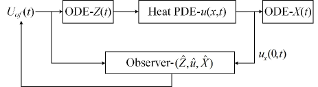
Figure 1: The output-feedback closed-loop system consisting of the plant (1)-(5), observer (88)-(91) and control input (145).

Theorem 5.

Suppose that the matrices $A,A_{z}$ have no eigenvalues of the form $-\bar{k}^{2}\pi^{2}$, for $\bar{k}\in N$. For any initial value $(u(x,0),\hat{u}(x,0))\in H^{{2m}}(0,1)\times H^{{2m}}(0,1)$, the output-feedback closed-loop system consisting of the plant-$(u(x,t),X(t),Z(t))$ (1)-(5), the observer-$(\hat{u}(x,t),\hat{X}(t),\hat{Z}(t))$ (88)-(91) and the control input (145) has the following properties:

$i$). There exist positive constants $\Upsilon_{all}$ and $\lambda_{all}$ such that

$$\bar{\Omega}(t)\leq\Upsilon_{all}\left(\bar{\Omega}(0)^{2}+|\delta(0)|^{2}+\tilde{u}_{x}(0,0)^{2}\right)^{\frac{1}{2}}e^{-\lambda_{all}t}$$ (146)

where

$$\bar{\Omega}(t)=\bigg{(}\|{{u}(\cdot,t)}\|^{2}+\|{u_{x}}(\cdot,t)\|^{2}+{\left|{X(t)}\right|^{2}}+\left|{Z(t)}\right|^{2}$$

$$+\|{{\hat{u}}(\cdot,t)}\|^{2}+\|{\hat{u}_{x}}(\cdot,t)\|^{2}+{\left|{\hat{X}(t)}\right|^{2}}+\left|{\hat{Z}(t)}\right|^{2}\bigg{)}^{\frac{1}{2}},$$ (147)

and $\delta(t)$ will be shown later.

$ii$). The output-feedback control law (145), $|U_{of}(t)|$ is bounded by ${\Upsilon_{of}}$ and is exponentially convergent to zero in the sense of $|U_{of}(t)|\leq{\Upsilon_{of}}e^{-{\lambda_{of}}t}$ with positive constants $\lambda_{of}$ and $\Upsilon_{of}$ which only depends on initial values of the system.

Proof.

Proof of property $i$): Inserting the output-feedback control law (145) into (5), adding and subtracting terms, we have

$$\dot{Z}(t) ={A_{z}}Z(t)+{B_{z}}U(t)+B_{z}\delta(t),$$ (148)

where

$$\delta(t)= \mathcal{L}\tilde{u}(1,t)-\mathcal{C}\tilde{u}(0,t)-\left(\mathcal{L}\Phi(1)-\mathcal{C}\Phi(0)\right)\tilde{X}(t)$$

$$-\mathcal{L}\int_{0}^{1}{{\phi}}(1,y)\tilde{u}(y,t)dy$$

$$+\tilde{F}\left(\tilde{u}(0,t),\cdots,\partial_{x}^{2m-2}\tilde{u}(0,t)\right)$$ (149)

with $\tilde{F}=\left(\mathcal{C}\int_{0}^{x}{{\phi}}(x,y)\tilde{u}(y,t)dy\right)|_{x=0}$, and $U(t)$ is in the state-feedback form (64).

Recalling Theorem 4, we have $\delta(t)$ (149) is exponentially convergent to zero. Together with Theorem 2, we obtain the exponential stability result as

$$\quad\|u(\cdot,t)\|^{2}+\|u_{x}(\cdot,t)\|^{2}+|X(t)|^{2}+|Z(t)|^{2}$$

$$\leq\|u(\cdot,t)\|^{2}+\|u_{x}(\cdot,t)\|^{2}+|X(t)|^{2}+|Z(t)|^{2}+|\delta(t)|^{2}$$

$$\leq\Upsilon_{uo}\bigg{(}\|u(\cdot,0)\|^{2}+\|u_{x}(\cdot,0)\|^{2}+|X(0)|^{2}$$

$$\quad+|Z(0)|^{2}+|\delta(0)|^{2}\bigg{)}e^{-\lambda_{uo}t},$$ (150)

for some positive $\Upsilon_{uo},\lambda_{uo}$.

Recalling Theorem 4 and (92), we obtain

$$\|\hat{u}(\cdot,t)\|^{2}+\|\hat{u}_{x}(\cdot,t)\|^{2}+|\hat{X}(t)|^{2}+|\hat{Z}(t)|^{2}$$

$$\leq \hat{\xi}_{0}\bigg{(}\|u(\cdot,t)\|^{2}+\|u_{x}(\cdot,t)\|^{2}+|X(t)|^{2}+|Z(t)|^{2}$$

$$+\|\tilde{u}(\cdot,t)\|^{2}+\|\tilde{u}_{x}(\cdot,t)\|^{2}+|\tilde{X}(t)|^{2}+|\tilde{Z}(t)|^{2}\bigg{)}$$

$$\leq \Upsilon_{\hat{u}}\bigg{(}\|u(\cdot,0)\|^{2}+\|u_{x}(\cdot,0)\|^{2}+|X(0)|^{2}+|Z(0)|^{2}+|\delta(0)|^{2}$$

$$+\|\tilde{u}(\cdot,0)\|^{2}+\|\tilde{u}_{x}(\cdot,0)\|^{2}+|\tilde{X}(0)|^{2}+|\tilde{Z}(0)|^{2}$$

$$+\tilde{u}_{x}(0,0)^{2}\bigg{)}e^{-\lambda_{\hat{u}}t},$$ (151)

for some positive $\hat{\xi}_{0},\Upsilon_{\hat{u}},\lambda_{\hat{u}}$. With representing the initial values $\|\tilde{u}(\cdot,0)\|^{2}+\|\tilde{u}_{x}(\cdot,0)\|^{2}+|\tilde{X}(0)|^{2}+|\tilde{Z}(0)|^{2}$ as $\|u(\cdot,0)\|^{2}+\|u_{x}(\cdot,0)\|^{2}+|X(0)|^{2}+|Z(0)|^{2}$+$\|\hat{u}(\cdot,0)\|^{2}+\|\hat{u}_{x}(\cdot,0)\|^{2}+|\hat{X}(0)|^{2}+|\hat{Z}(0)|^{2}$ by recalling (92) and using Cauchy-Schwarz inequality, Property $i$) can then be proved.

Proof of property $ii$): Recalling the exponential stability estimates $\sum_{i=0}^{2m}\|\partial_{x}^{i}u(\cdot,t)\|$ and $\sum_{i=0}^{2m}\|\partial_{x}^{i}\tilde{u}(\cdot,t)\|$ proved by Theorem 2, Lemma 1 and Theorem 4, we have the exponential stability estimate in the sense of the norm $\sum_{i=0}^{2m}\|\partial_{x}^{i}\hat{u}(\cdot,t)\|$. Using Sobolev inequality, we obtain the exponential stability estimate in term of the norm $\|\hat{u}(\cdot,t)\|_{C_{2m-1}}$, together with the property $i$), which give the exponential convergence of $U_{of}(t)$ which uses the signals $\sum_{i=0}^{2m-1}\partial_{x}^{i}\hat{u}(1,t)$, $\sum_{i=0}^{2m-1}\partial_{x}^{i}\hat{u}(0,t)$, $\hat{X}(t)$ and $\hat{u}(x,t)$.

The proof of Theorem 5 is completed. ∎

V Simulation

Consider the simulation example where the plant coefficients in (1)-(5) are $A=[1,1;1,0.5]$, $A_{z}=[0,1;1,1]$, $B_{z}=B=[0,1]^{T}$, $C_{X}=C_{z}=[1,0]^{T}$ and $q=1$. Two ODEs sandwiching the heat PDE are considered as two-order systems here, i.e., $m=2$ in the above design and analysis, because the second-order ODE is a classic system which can describe many actuator and sensor dynamics. The simulation is conducted based on the finite difference method with dividing the spatial and time domains into a grid as $x_{0},\cdots,x_{f}$ and $t_{0},\cdots,t_{n^{*}}$ respectively, where the time step and space step sizes are $0.001$ and $0.05$. The initial conditions of the plant are defined as $u(x,0)=\sin(2\pi x)$, $X(0)=[x_{1}(0),x_{2}(0)]^{T}=[u(0,0),0]^{T}$, $Z(0)=[z_{1}(0),z_{2}(0)]^{T}=[u(1,0),0]^{T}$. The initial conditions of the observer (88)-(91) are $\hat{u}(x,0)=0$, $\hat{X}(0)=\hat{Z}(0)=[0,0]^{T}$. Choose the control parameters $c_{1}=c_{2}=3$, $K=[-10,-5]$, $P_{0}=[-2,-4]^{T}$ and $P_{2}=[-4,-12]^{T}$. Apply the output-feedback control law (145) with $m=2$, which is constructed by the states $\sum_{i=0}^{3}\partial_{x}^{i}\hat{u}(1,t)$, $\sum_{i=0}^{3}\partial_{x}^{i}\hat{u}(0,t)$, $\hat{X}(t)$ and $\hat{u}(x,t)$ of the observer (88)-(91) built using the measurement $u_{x}(0,t)$, into the plant (1)-(5). Note that the third-order spatial derivatives are determined by finite difference method such as

$$\quad\hat{u}_{xxx}(1,t_{j})$$

$$=\frac{\hat{u}(x_{f},t_{j})-3\hat{u}(x_{f-1},t_{j})+3\hat{u}(x_{f-2},t_{j})-\hat{u}(x_{f-3},t_{j})}{\Delta h^{3}},$$ (152)

where $\Delta h$ is spatial step size and $t_{j}$ is the current time point. $\hat{u}_{xxx}(1,t_{j})$ is used to determine $U(t_{j+1})$.

The responses of the output-feedback closed-loop system are shown following.

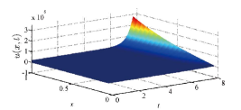
(a) uncontrolled case.

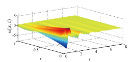
(b) controlled case.

Figure 2: Responses of the heat PDE states $u(x,t)$ in the uncontrolled case and under the output-feedback control law (145).

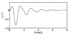
(a) $x_{1}(t)$.

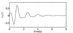
(b) $x_{2}(t)$.

Figure 3: Responses of the ODE state $X(t)$ under the output-feedback control law (145).

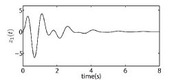
(a) $z_{1}(t)$.

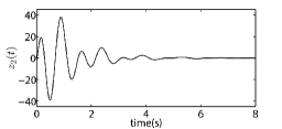
(b) $z_{2}(t)$.

Figure 4: Responses of the ODE state $Z(t)$ under the output-feedback control law (145).

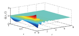
(a) observer error.

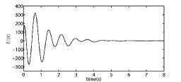
(b) control input.

Figure 5: a) Observer errors $\tilde{u}=u-\hat{u}$ of the observer (88)-(91). b) The output-feedback control input (145).

As Fig.2 shows, the response $u(x,t)$ of the heat PDE exhibits unstable behaviour in the uncontrolled case while the convergent manner of the response $u(x,t)$ is achieved when we apply the proposed output feedback control law (145). Similarly, Figs. 3-4 show the ODE states $X(t)=[x_{1}(t),x_{2}(t)]^{T}$ and $Z(t)=[z_{1}(t),z_{2}(t)]^{T}$ are also convergent to zero in the output-feedback closed-loop system. It can be seen in Fig. 5 a) that the observer errors $\tilde{u}(x,t)=u(x,t)-\hat{u}(x,t)$ also converge fast to zero in the closed-loop system. Moreover, Fig. 5 b) shows the output-feedback control input are bounded and convergent to zero.

VI Conclusion and Future work

In this paper, we present a methodology combining PDE backstepping and ODE backstepping to stabilize a parabolic PDE sandwiched between two arbitrary-order ODEs. An observer is also designed only using one PDE boundary value $u_{x}(0,t)$ to reconstruct all PDE and ODE states. The observer-based output-feedback control law is proposed and the exponential stability of the closed-loop system is proved via Lyapunov analysis. Moreover, the boundedness and exponential convergence of the designed control input is also proved in this paper. These theoretical results are verified via the simulation as well. In the future work, more general ODE dynamics in the input channel will be considered in the control design.

VII Appendix

Proof of Lemma 1:

VII-1 Proof of i)

Taking 2 and 3 times derivative of (15) with respect to $x$ respectively, we have

$$w_{txx}(x,t)=q\partial_{x}^{4}w(x,t),$$ (153)

$$w_{txxx}(x,t)=q\partial_{x}^{5}w(x,t).$$ (154)

Define a Lyapunov function

$$V_{2}(t)=R_{0}V(t)+\frac{a_{2}}{2}\|\partial_{x}^{2}w(\cdot,t)\|^{2}+\frac{a_{3}}{2}\|\partial_{x}^{3}w(\cdot,t)\|^{2},$$ (155)

where $a_{2},a_{3}$ are positive constants to be determined later.

Defining

$$\Omega_{1}(t)=\Omega(t)+\|\partial_{x}^{2}w(\cdot,t)\|^{2}+\|\partial_{x}^{3}w(\cdot,t)\|^{2}.$$ (156)

We have

$$\theta_{11}\Omega_{1}(t)\leq V_{2}(t)\leq\theta_{12}\Omega_{1}(t),$$ (157)

for some positive $\theta_{11},\theta_{12}$.

Taking the derivative of (155) along (153)-(154) and (16), recalling (83), applying Agmon’s inequality, Young’s inequality and Cauchy-Schwarz inequality, yields

$$\dot{V}_{2}(t)$$

$$\leq -R_{0}\lambda V(t)-\left(\frac{{{a_{3}}q}}{2}-\frac{1}{{4{r_{2}}}}{a_{2}}-\frac{1}{{4{r_{3}}}}\frac{{a_{3}}}{q}\right){w_{xxx}}(0,t)^{2}$$

$$-\left(({a_{2}}-{a_{3}})q-\frac{1}{{4{r_{2}}}}{a_{2}}-\frac{1}{{4{r_{3}}}}\frac{{a_{3}}}{q}\right){\left\|{{w_{xxx}}}\right\|^{2}}$$

$$-\left(\frac{1}{2}{a_{3}}q-\frac{1}{{4{r_{2}}}}{a_{2}}-\frac{1}{{4{r_{3}}}}\frac{{a_{3}}}{q}\right){\left\|{{w_{xxxx}}}\right\|^{2}}$$

$$+{r_{2}}{a_{2}}{w_{t}}{(1,t)^{2}}+{r_{3}}\frac{{a_{3}}}{q}{w_{tt}}{(1,t)^{2}}-R_{0}\bar{\xi}_{a}w_{x}(0,t)^{2},$$ (158)

where $r_{2},r_{3}$ are positive constants from Young’s inequality to be chosen later.

Recalling (48)-(50) and (76)-(77), considering the case of $m\geq 3$, we have

$$\dot{V}_{2}(t)\leq -\frac{R_{0}}{2}\lambda V(t)$$

$$-\left(\frac{{{a_{3}}q}}{2}-\frac{1}{{4{r_{2}}}}{a_{2}}-\frac{1}{{4{r_{3}}}}\frac{{a_{3}}}{q}\right){w_{xxx}}(0,t)^{2}$$

$$-\left(({a_{2}}-{a_{3}})q-\frac{1}{{4{r_{2}}}}{a_{2}}-\frac{1}{{4{r_{3}}}}\frac{{a_{3}}}{q}\right){\left\|{{w_{xxx}}}\right\|^{2}}$$

$$-\left(\frac{1}{2}{a_{3}}q-\frac{1}{{4{r_{2}}}}{a_{2}}-\frac{1}{{4{r_{3}}}}\frac{{a_{3}}}{q}\right){\left\|{{w_{xxxx}}}\right\|^{2}}$$

$$-\left(\frac{R_{0}}{2}\lambda\theta_{1}-2{r_{2}}{a_{2}}c_{1}^{2}-3{r_{3}}\frac{1}{q}{a_{3}}(c_{1}^{2}-1)^{2}\right)y_{1}(t)^{2}$$

$$-\left(\frac{R_{0}}{2}\lambda\theta_{1}-3{r_{3}}\frac{1}{q}{a_{3}}(c_{1}+c_{2})^{2}-2{r_{2}}{a_{2}}\right)y_{2}(t)^{2}$$

$$-\left(\frac{R_{0}}{2}\lambda\theta_{1}-3{r_{3}}\frac{1}{q}{a_{3}}\right)y_{3}(t)^{2}.$$ (159)

Choosing $a_{2}>a_{3}$ and sufficiently large ${r_{2}}$, ${r_{3}}$, $R_{0}$, we arrive at

$$\dot{V}_{2}(t)\leq -\frac{R_{0}}{2}\lambda V(t)$$

$$-\frac{1}{5}\left(({a_{2}}-{a_{3}})q-\frac{1}{{4{r_{2}}}}{a_{2}}-\frac{1}{{4{r_{3}}}}\frac{{a_{3}}}{q}\right)$$

$$\quad\times\left({\left\|{{w_{xx}}}\right\|^{2}}+{\left\|{{w_{xxx}}}\right\|^{2}}\right),$$ (160)

where Poincar$\acute{e}$ inequality is used. Therefore, we obtain

$$\dot{V}_{2}(t)\leq-\lambda_{2}V_{2}(t)$$ (161)

for some positive $\lambda_{2}$. Recalling (157) and invertibility of the backstepping transformations, we obtain $i)$ in Lemma 1.

In the case of $m=2$: (84) and Cauchy-Schwarz inequality can be used to rewrite $\frac{{r_{3}}{a_{3}}}{q}w_{tt}(1,t)^{2}$ in (159) as $\frac{{r_{3}}a_{3}}{q}{}(\xi_{b}w(1,t)^{2}$+$\xi_{b}w_{t}(1,t)^{2}$+$\xi_{b}|X(t)|^{2}$+$\xi_{b}\|w\|^{2})$ with some positive $\xi_{b}$, where $-\frac{R_{0}}{2}\lambda\theta_{1}(y_{1}(t)^{2}+y_{2}(t)^{2})$ and $-\frac{R_{0}}{2}\lambda\theta_{1}(|X(t)|^{2}+\|w\|^{2})$ derived from $-\frac{R_{0}}{2}\lambda V(t)$ with large enough $R_{0}$ can “cancel” $\frac{{r_{3}}a_{3}}{q}\xi_{b}w(1,t)^{2}$, $(\frac{{r_{3}}a_{3}}{q}\xi_{b}+r_{2}a_{2})w_{t}(1,t)^{2}$ according to (48)-(49), and $\frac{{r_{3}}a_{3}}{q}\xi_{b}|X(t)|^{2}$, $\frac{{r_{3}}a_{3}}{q}\xi_{b}\|w\|^{2}$ respectively. (161) can then also be obtained.

In the case of $m=1$: substituting $m=1$ into (84) and taking the time derivative, applying Cauchy-Schwarz inequality and recalling (85), we have

$$w_{tt}(1,t)^{2} =\xi_{c}\|w_{xx}\|^{2}+\xi_{c}|X(t)|^{2}+\xi_{c}w_{x}(0,t)^{2}$$

$$\quad+\xi_{c}w(1,t)^{2}+\xi_{c}\|w\|^{2}.$$ (162)

Substituting (85) and (162) with (48) into (158), we can obtain

$$\dot{V}_{2}(t)\leq-\frac{R_{0}}{2}\lambda V(t)-\left(R_{0}\bar{\xi}_{a}-\frac{{r_{3}}{a_{3}}\xi_{c}}{q}\right)w_{x}(0,t)^{2}$$

$$-\left(\frac{{{a_{3}}q}}{2}-\frac{1}{{4{r_{2}}}}{a_{2}}-\frac{1}{{4{r_{3}}}}\frac{{a_{3}}}{q}\right){w_{xxx}}(0,t)^{2}$$

$$-\left(({a_{2}}-{a_{3}})q-\frac{1}{{4{r_{2}}}}{a_{2}}-\frac{1}{{4{r_{3}}}}\frac{{a_{3}}}{q}\right){\left\|{{w_{xxx}}}\right\|^{2}}$$

$$-\left(\frac{1}{2}{a_{3}}q-\frac{1}{{4{r_{2}}}}{a_{2}}-\frac{1}{{4{r_{3}}}}\frac{{a_{3}}}{q}\right){\left\|{{w_{xxxx}}}\right\|^{2}}$$

$$-\left(\frac{R_{0}}{2}\lambda\theta_{1}-{r_{2}}{a_{2}}\xi_{a}-\frac{{r_{3}}{a_{3}}\xi_{c}}{q}\right)y_{1}(t)^{2}$$

$$-\left(\frac{R_{0}}{2}\lambda\theta_{1}-{r_{2}}{a_{2}}\xi_{a}-\frac{{r_{3}}{a_{3}}\xi_{c}}{q}\right)|X(t)|^{2}$$

$$-\left(\frac{R_{0}}{2}\lambda\theta_{1}-{r_{2}}{a_{2}}\xi_{a}-\frac{{r_{3}}{a_{3}}\xi_{c}}{q}\right)\|w\|^{2}+\frac{{r_{3}}{a_{3}}\xi_{c}}{q}\|w_{xx}\|^{2}.$$ (163)

Choosing sufficiently large $R_{0}$ and using Poincar$\acute{e}$ inequality, we have

$$\dot{V}_{2}(t)\leq-\frac{R_{0}}{2}\lambda V(t)$$

$$-\left(\frac{{{a_{3}}q}}{2}-\frac{1}{{4{r_{2}}}}{a_{2}}-\frac{1}{{4{r_{3}}}}\frac{{a_{3}}}{q}\right)({w_{xxx}}(0,t)^{2}+\|w_{xxxx}\|^{2})$$

$$-\left(\frac{1}{5}({a_{2}}-{a_{3}})q-\frac{1}{{20{r_{2}}}}{a_{2}}-\frac{1}{{20{r_{3}}}}\frac{{a_{3}}}{q}\right){\left\|{{w_{xxx}}}\right\|^{2}}$$

$$-\left(\frac{1}{5}({a_{2}}-{a_{3}})q-\frac{1}{{20{r_{2}}}}{a_{2}}-\frac{1}{{20{r_{3}}}}\frac{{a_{3}}}{q}-\frac{{r_{3}}{a_{3}}\xi_{c}}{q}\right)\|w_{xx}\|^{2}.$$ (164)

In order to make the coefficients before $w_{xxx}(0,t)^{2}+\|w_{xxxx}\|^{2}$, $\|w_{xxx}\|^{2}$ and $\|w_{xx}\|^{2}$ positive, $a_{2},a_{3}$ and $r_{2},r_{3}$ should be chosen satisfying

$$\frac{\frac{q}{5}+\frac{1}{20r_{3}q}+\frac{r_{3}\xi_{c}}{q}}{\frac{q}{5}-\frac{1}{20r_{2}}}a_{3}<a_{2}<4r_{2}\left(\frac{q}{2}-\frac{1}{4qr_{3}}\right)a_{3},$$ (165)

$$r_{3}>\frac{1}{2q^{2}},~{}~{}r_{2}>\frac{\frac{1}{4}+\frac{1}{16r_{3}q^{2}}+\frac{5r_{3}\xi_{c}}{4q^{2}}}{\frac{q}{2}-\frac{1}{4qr_{3}}}+\frac{1}{4q}.$$ (166)

(161) is thus obtained as well in the case of $m=1$.

Therefore, (161) can be obtained when $m\geq 1$. The proof of the first result in Lemma 1 is completed.

VII-2 Proof of ii)

Through similar processes from (153) to (161), we can obtain the exponential stability estimates in the sense of $(\|\partial_{x}^{4}w(\cdot,t)\|^{2}+\|\partial_{x}^{5}w(\cdot,t)\|^{2})^{\frac{1}{2}}$, $(\|\partial_{x}^{6}w(\cdot,t)\|^{2}+\|\partial_{x}^{7}w(\cdot,t)\|^{2})^{\frac{1}{2}}$ and so on, i.e., the exponential stability estimates in the sense of $(\|\partial_{x}^{4}u(\cdot,t)\|^{2}+\|\partial_{x}^{5}u(\cdot,t)\|^{2})^{\frac{1}{2}}$, $(\|\partial_{x}^{6}u(\cdot,t)\|^{2}+\|\partial_{x}^{7}u(\cdot,t)\|^{2})^{\frac{1}{2}}$ and so on, because of the invertibility of the backstepping transformation.

Next, we prove the exponential stability estimate in the sense of $(\|\partial_{x}^{2m-2}u(\cdot,t)\|^{2}+\|\partial_{x}^{2m-1}u(\cdot,t)\|^{2})^{\frac{1}{2}}$.

Taking $2m-2$ and $2m-1$ times derivative of (15) with respect to $x$ respectively, we have

$$\partial_{x}^{2m-2}w_{t}(x,t) =q\partial_{x}^{2m}w(x,t),$$ (167)

$$\partial_{x}^{2m-1}w_{t}(x,t) =q\partial_{x}^{2m+1}w(x,t).$$ (168)

Apply a Lyapunov function

$${V_{{\rm{2m-2}}}}(t)=\frac{{{a_{2m-2}}}}{2}\|{\partial_{x}^{2m-2}{w}}(\cdot,t)\|^{2}+\frac{{{a_{2m-1}}}}{2}\|{\partial_{x}^{2m-1}{w}}(\cdot,t)\|^{2}.$$ (169)

Taking the derivative of (169), we have

$${{\dot{V}}_{2m-2}}(t)$$

$$\leq -\bigg{(}\frac{{{a_{2m-1}}q}}{2}-\frac{{a_{2m-2}}}{{4q^{m-2}{r_{2m-2}}}}$$

$$\quad-\frac{{a_{2m-1}}}{{4q^{m-1}{r_{2m-1}}}}\bigg{)}{\partial_{x}^{2m-1}w(0,t)}^{2}$$

$$-\bigg{(}({a_{2m-2}}-{a_{2m-1}})q-\frac{{a_{2m-2}}}{{4q^{m-2}{r_{2m-2}}}}$$

$$\quad-\frac{{a_{2m-1}}}{{4q^{m-1}{r_{2m-1}}}}\bigg{)}{\left\|{\partial_{x}^{2m-1}w}\right\|^{2}}$$

$$-\bigg{(}\frac{{a_{2m-1}}q}{2}-\frac{{a_{2m-2}}}{{4q^{m-2}{r_{2m-2}}}}-\frac{{a_{2m-1}}}{{4q^{m-1}{r_{2m-1}}}}\bigg{)}{\left\|{\partial_{x}^{2m}w}\right\|^{2}}$$

$$+\frac{{r_{2m-2}}{a_{2m-2}}}{{{q^{m-2}}}}{\partial_{t}^{m-1}{w}(1,t)}^{2}+\frac{{r_{2m-1}}{a_{2m-1}}}{{{q^{m-1}}}}{\partial_{t}^{m}w(1,t)}^{2}.$$

Note that ${\partial_{x}^{2m-1}w(0,t)}^{2}\triangleq(\partial_{x}^{2m-1}w(x,t)|_{x=0})^{2}$ and ${\partial_{t}^{m}w(1,t)}^{2}\triangleq(\partial_{t}^{m}w(x,t)|_{x=1})^{2}$.

We choose $a_{2m-2}>a_{2m-1}$ and sufficiently large ${r_{2m-2}}$, ${r_{2m-1}}$ to make

$$\quad\dot{V}_{2m-2}(t)$$

$$\leq-\frac{1}{5}\bigg{(}({a_{2m-2}}-{a_{2m-1}})q-\frac{{a_{2m-2}}}{{4q^{m-2}{r_{2m-2}}}}$$

$$\quad-\frac{{a_{2m-1}}}{{4q^{m-1}{r_{2m-1}}}}\bigg{)}\left({\left\|{\partial_{x}^{2m-1}w}\right\|^{2}}+\left\|{\partial_{x}^{2m-2}w}\right\|^{2}\right)$$

$$\quad+\frac{{r_{2m-2}}{a_{2m-2}}}{{{q^{m-2}}}}{\partial_{t}^{m-1}{w}(1,t)}^{2}+\frac{{r_{2m-1}}{a_{2m-1}}}{{{q^{m-1}}}}{\partial_{t}^{m}w(1,t)}^{2}$$

$$\leq-\bar{\lambda}_{2m-2}V_{2m-2}(t)+\frac{{r_{2m-2}}{a_{2m-2}}}{{{q^{m-2}}}}{\partial_{t}^{m-1}{w}(1,t)}^{2}$$

$$\quad+\frac{{r_{2m-1}}{a_{2m-1}}}{{{q^{m-1}}}}{\partial_{t}^{m}w(1,t)}^{2},$$ (170)

for some positive $\lambda_{2m-2}$, where Poincar$\acute{e}$ inequality is used.

Applying Cauchy-Schwarz inequality into (84), we have

$$\left|\partial_{t}^{m}w(1,t)\right|^{2}\leq\xi\|w\|^{2}+\xi|X(t)|^{2}+\xi\sum_{i=0}^{m-1}\left|\partial_{t}^{i}w(1,t)\right|^{2}$$ (171)

with some positive $\xi$. By recalling (48)-(50), (76)-(77) and (83), we obtain the exponential convergence of $\partial_{t}^{m}w(1,t)$ via (171), i.e.,

$$\left|\partial_{t}^{m}w(1,t)\right|\leq\bar{\Upsilon}_{m}e^{-\xi_{1}t}=\eta_{m}(t),$$ (172)

for some positive $\bar{\Upsilon}_{m}$ and $\xi_{1}$.

Define a Lyapunov function

$${V_{u1}}(t) =V_{2m-2}(t)+\bar{R}_{0}V(t)+\frac{\bar{R}_{1}}{2}\eta_{m}(t)^{2},$$ (173)

where $\bar{R}_{0},\bar{R}_{1}$ are positive constants to be determined later.

Taking the derivative of (173) and recalling (83), (170), (172), we have

$$\dot{V}_{u1}(t)\leq-\bar{\lambda}_{2m-2}V_{2m-2}(t)+\frac{{r_{2m-2}}{a_{2m-2}}}{{{q^{m-2}}}}{\partial_{t}^{m-1}{w}(1,t)}^{2}$$

$$\quad-\left(\bar{R}_{1}\xi_{1}-\frac{{r_{2m-1}}{a_{2m-1}}}{{{q^{m-1}}}}\right)\eta_{m}(t)^{2}-\bar{R}_{0}\lambda V(t).$$ (174)

Choosing large enough $\bar{R}_{0},\bar{R}_{1}$, we obtain

$$\dot{V}_{u1}(t)\leq-\lambda_{u1}V_{u1}(t)$$ (175)

for some positive $\lambda_{u1}$, where $-y_{1}^{2},\cdots,-y_{m}^{2}$ in $-\frac{\bar{R}_{0}}{2}\lambda V(t)$ extracted from $-{\bar{R}_{0}}\lambda V(t)$ are used to “cancel” ${\partial_{t}^{m-1}{w}(1,t)}^{2}$ by recalling (76)-(77) and (48)-(50).

Therefore, we obtain the exponential stability estimate in the sense of $(\|\partial_{x}^{2m-2}u(\cdot,t)\|^{2}+\|\partial_{x}^{2m-1}u(\cdot,t)\|^{2})^{\frac{1}{2}}$ by recalling (175), (173), (169) and the invertibility of the backstepping transformation.

Next, we prove the exponential stability estimate in the sense of $(\|\partial_{x}^{2m}u(\cdot,t)\|^{2}+\|\partial_{x}^{2m+1}u(\cdot,t)\|^{2})^{\frac{1}{2}}$.

Taking $2m$ and $2m+1$ times derivative of (15) with respect to $x$ respectively, we have

$$\partial_{x}^{2m}w_{t}(x,t) =q\partial_{x}^{2m+2}w(x,t),$$ (176)

$$\partial_{x}^{2m+1}w_{t}(x,t) =q\partial_{x}^{2m+3}w(x,t).$$ (177)

Consider now a Lyapunov function

$${V_{{\rm{2m}}}}(t)=\frac{{{a_{2m}}}}{2}\|{\partial_{x}^{2m}{w}}(\cdot,t)\|^{2}+\frac{{{a_{2m+1}}}}{2}\|{\partial_{x}^{2m+1}{w}}(\cdot,t)\|^{2},$$

where the positive parameters $a_{2m},a_{2m+1}$ are to be chosen later. Taking the derivative of $V_{2m}(t)$ along the (176)-(177) as

$$\dot{V}_{2m}(t)\leq-\bigg{(}({a_{2m}}-{a_{2m+1}})q-\frac{{a_{2m}}}{{4{q^{m-1}}{r_{2m}}}}$$

$$\quad-\frac{{a_{2m+1}}}{{4{q^{m}}{r_{2m+1}}}}\bigg{)}{\left\|{\partial_{x}^{2m+1}w}\right\|^{2}}-\bigg{(}\frac{1}{2}{a_{2m+1}}q$$

$$\quad-\frac{{a_{2m}}}{{4{q^{m-1}}{r_{2m}}}}-\frac{{a_{2m+1}}}{{4{q^{m}}{r_{2m+1}}}}\bigg{)}{\left\|{\partial_{x}^{2m+2}w}\right\|^{2}}$$

$$\quad-\bigg{(}\frac{{{a_{2m+1}}q}}{2}-\frac{{a_{2m}}}{{4{q^{m-1}}{r_{2m}}}}-\frac{{a_{2m+1}}}{{4{q^{m}}{r_{2m+1}}}}\bigg{)}{\partial_{x}^{2m+1}{w}(0,t)}^{2}$$

$$\quad+\frac{{r_{2m}}{a_{2m}}}{{{q^{m-1}}}}{\partial_{t}^{m}w(1,t)}^{2}+\frac{{r_{2m+1}}{a_{2m+1}}}{{{q^{m}}}}{\partial_{t}^{m+1}w(1,t)}^{2}.$$

We choose $a_{2m}>a_{2m+1}$ and sufficiently large ${r_{2m}}$, ${r_{2m+1}}$ to make

$$\dot{V}_{2m}(t)\leq-\frac{1}{5}\bigg{(}({a_{2m}}-{a_{2m+1}})q-\frac{{a_{2m}}}{{4{q^{m-1}}{r_{2m}}}}$$

$$\quad-\frac{{a_{2m+1}}}{{4{q^{m}}{r_{2m+1}}}}\bigg{)}\left({\left\|{\partial_{x}^{2m}w}\right\|^{2}}+{\left\|{\partial_{x}^{2m+1}w}\right\|^{2}}\right)$$

$$\quad+\frac{{r_{2m}}{a_{2m}}}{{{q^{m-1}}}}{\partial_{t}^{m}w(1,t)}^{2}+\frac{{r_{2m+1}}{a_{2m+1}}}{{{q^{m}}}}{\partial_{t}^{m+1}w(1,t)}^{2},$$

where Poincar$\acute{e}$ inequality is used.

We thus have

$$\dot{V}_{2m}(t) \leq-\bar{\lambda}_{2m}V_{2m}(t)+\frac{{r_{2m}}{a_{2m}}}{{{q^{m-1}}}}{\partial_{t}^{m}w(1,t)}^{2}$$

$$\quad+\frac{{r_{2m+1}}{a_{2m+1}}}{{{q^{m}}}}{\partial_{t}^{m+1}w(1,t)}^{2},$$ (178)

for some positive $\bar{\lambda}_{2m}$.

Taking the time derivative of (84) and using Cauchy-Schwarz inequality, we have

$$\left|\partial_{t}^{m+1}w(1,t)\right|^{2}\leq \xi_{0}\|w_{xx}(\cdot,t)\|^{2}+\xi_{0}|X(t)|^{2}$$

$$+\xi_{0}w_{x}(0,t)^{2}+\xi_{0}\sum_{i=1}^{m}\left|\partial_{t}^{i}w(1,t)\right|^{2}$$ (179)

for some positive $\xi_{0}$, where (14) is used. Recalling (76), (156)-(157), (161), we have the exponential stability estimate in the sense of $\sum_{i=0}^{2}\|\partial_{x}^{i}w(\cdot,t)\|$. Using Sobolev inequality, we obtain the exponential stability estimate in term of the norm $\|w(\cdot,t)\|_{C_{1}}$. Together with (48)-(50), (76), (156)-(157), (161) and (172), we have the exponential convergence of $\partial_{t}^{m+1}w(1,t)$ via (179), i.e.,

$$\left|\partial_{t}^{m+1}w(1,t)\right|\leq\bar{\Upsilon}_{m+1}e^{-\xi_{2}t}=\eta_{m+1}(t),$$ (180)

for some positive $\bar{\Upsilon}_{m+1}$ and $\xi_{2}$.

Define a Lyapunov function

$${V_{u}}(t) =V_{2m}(t)+\frac{R_{1}}{2}\eta_{m}(t)^{2}+\frac{R_{2}}{2}\eta_{m+1}(t)^{2},$$ (181)

where $R_{1},R_{2}$ are positive constants to be determined later.

Defining

$$\Omega_{m}(t) =\|\partial_{x}^{2m}w(\cdot,t)\|^{2}+\|\partial_{x}^{2m+1}w(\cdot,t)\|^{2}$$

$$\quad+\eta_{m}(t)^{2}+\eta_{m+1}(t)^{2},$$ (182)

we have

$$\theta_{m1}\Omega_{m}(t)\leq V_{u}(t)\leq\theta_{m2}\Omega_{m}(t),$$ (183)

where ${\theta_{m1}}=\min\left\{\frac{a_{2m}}{2},\frac{a_{2m+1}}{2},\frac{R_{1}}{2},\frac{R_{2}}{2}\right\}$, ${\theta_{m2}}=\max\left\{\frac{a_{2m}}{2},\frac{a_{2m+1}}{2},\frac{R_{1}}{2},\frac{R_{2}}{2}\right\}$.

Taking the derivative of (181), recalling (178), (172), (180), we obtain

$$\dot{V}_{u}(t) \leq-\bar{\lambda}_{2m}V_{2m}(t)-\bigg{(}R_{1}\xi_{1}-\frac{{r_{2m}}{a_{2m}}}{{{q^{m-1}}}}\bigg{)}\eta_{m}(t)^{2}$$

$$\quad-\bigg{(}R_{2}\xi_{2}-\frac{{r_{2m+1}}{a_{2m+1}}}{{{q^{m}}}}\bigg{)}\eta_{m+1}(t)^{2}.$$ (184)

Choosing large sufficiently $R_{1},R_{2}$, we arrive at

$$\dot{V}_{u}(t)\leq-\lambda_{u}V_{u}(t)$$ (185)

for some positive $\lambda_{u}$.

Now we obtain the exponential stability estimate in the sense of the norm $\Omega_{m}(t)^{\frac{1}{2}}$ recalling (182)-(183). Using the invertibility of (12), we obtain the exponential stability estimate in the sense of $(\|\partial_{x}^{2m}u(\cdot,t)\|^{2}+\|\partial_{x}^{2m+1}u(\cdot,t)\|^{2})^{\frac{1}{2}}$.

Therefore, using the result in the subsection $1)$ and the above proof in the subsection $2)$, we obtain $ii)$ of Lemma 1.

The proof of Lemma 1 is completed.

Proof of Theorem 4: Define a Lyapunov function

$$V_{w}(t)=\sum\limits_{i=0}^{2m}\|\partial_{x}^{i}\tilde{w}(\cdot,t)\|^{2}.$$ (186)

Taking $i$ times derivative of (98) with respect to $x$,

$$\partial_{x}^{i}\tilde{w}_{t}(x,t)=q\partial_{x}^{i}\tilde{w}_{xx}(x,t),$$ (187)

where $i=1,\cdots,2m$. Taking the derivative of (186) along (98)-(99) and (187), applying Poincar$\acute{e}$ inequality, yields

$$\dot{V}_{w}(t) =-q\sum\limits_{i=1}^{2m+1}\|\partial_{x}^{i}\tilde{w}(\cdot,t)\|^{2}$$

$$\leq-\frac{1}{5}q\sum\limits_{i=0}^{2m}\|\partial_{x}^{i}\tilde{w}(\cdot,t)\|^{2}\leq-\lambda_{w}V_{w}(t),$$ (188)

for some positive $\lambda_{w}$.

We thus obtain

$$\sum_{i=0}^{2m}\|\partial_{x}^{i}\tilde{w}(\cdot,t)\|^{2}\leq \Upsilon_{\tilde{w}}\bigg{(}\sum_{i=0}^{2m}\|\partial_{x}^{i}\tilde{u}(\cdot,0)\|^{2}$$

$$+\left|\tilde{Z}(0)\right|^{2}+\left|\tilde{X}(0)\right|^{2}\bigg{)}e^{-\lambda_{\tilde{w}}t},$$ (189)

with $\Upsilon_{\tilde{w}},\lambda_{\tilde{w}}$ are some positive constants, where (97) is used to replace $\sum_{i=0}^{2m}\|\partial_{x}^{i}\tilde{w}(\cdot,0)\|^{2}$.

Especially from the exponential stability result of $\sum_{i=0}^{2}\|\partial_{x}^{i}\tilde{w}(\cdot,t)\|$ and using Sobolev inequality, we can obtain the exponential stability estimate in term of the norm $\|\tilde{w}(\cdot,t)\|_{C_{1}}$, which gives the exponential convergence of $\tilde{w}_{x}(0,t)$. Considering (113), because $\bar{A}$ (137) is Hurwitz and $\tilde{w}_{x}(0,t)$ is exponentially convergent, $|\tilde{Z}(t)|,|\tilde{X}(t)|$ are exponentially convergent in the sense of

$$\quad|\tilde{Z}(t)|^{2}+|\tilde{X}(t)|^{2}$$

$$\leq\Upsilon_{ZX}\left(|\tilde{Z}(0)|^{2}+|\tilde{X}(0)|^{2}+\tilde{u}_{x}(0,0)^{2}\right)e^{-\lambda_{ZX}t}$$ (190)

with $\Upsilon_{ZX},\lambda_{ZX}$ being some positive constants, where (97) is used to replace $\tilde{w}_{x}(0,0)^{2}$.

Recalling (97) and applying Cauchy-Schwarz inequality, we have

$$\sum_{i=0}^{2m}\|\partial_{x}^{i}\tilde{u}(\cdot,t)\|^{2}\leq 3\sum_{i=0}^{2m}\|\partial_{x}^{i}\tilde{w}(\cdot,t)\|^{2}+3\sum_{i=0}^{2m}\|\partial_{x}^{i}\vartheta(\cdot)\|^{2}\left|\tilde{Z}(t)\right|^{2}$$

$$+3\sum_{i=0}^{2m}\|\partial_{x}^{i}\theta(\cdot)\|^{2}\left|\tilde{X}(t)\right|^{2}.$$ (191)

Because $\sum_{i=0}^{2m}\|\partial_{x}^{i}\vartheta(\cdot)\|^{2}$ and $\sum_{i=0}^{2m}\|\partial_{x}^{i}\vartheta(\cdot)\|^{2}$ are bounded gains according to (128)-(134), applying (189)-(190), we obtain (143)-(144).

References

- [1] T. Ahmed-Ali, F. Giri, M. Krstic, F. Lamnabhi-Lagarrigue, “Observer design for a class of nonlinear ODE-PDE cascade systems”, Syst. Control Lett., 83, pp:19-27, 2015.
- [2] T. Ahmed-Ali, F. Giri, M. Krstic, F. Lamnabhi-Lagarrigue and L. Burlion, “Adaptive observer for a class of parabolic PDEs”, IEEE Trans. Autom. Control, 61(10), pp:3083-3090, 2016.
- [3] T. Ahmed-Ali, F. Giri, M. Krstic, L. Burlion and F. Lamnabhi-Lagarrigue, “Adaptive observer design with heat PDE sensor”, Automatica, 82, pp.93-100, 2017.
- [4] H. Anfinsen, O.M. Aamo, “Stabilization of a linear hyperbolic PDE with actuator and sensor dynamics”, Automatica, 95, 104-111, 2018.
- [5] A. Baccoli, A. Pisano and Y. Orlov. “Boundary control of coupled reaction-diffusion processes with constant parameters”, Automatica, 54, pp. 80-90, 2015.
- [6] M. B. Cheng, V. Radisavljevic, C. C. Chang, C. F. Lin and W. C. Su, “A sampled-data singularly perturbed boundary control for a heat conduction system with noncollocated observation”, IEEE Trans. Autom. Control, 54(6), 1305-1310, 2009.
- [7] J. Deutscher, “A backstepping approach to the output regulation of boundary controlled parabolic PDEs”, Automatica, 57, 56-64, 2015.
- [8] J. Deutscher,“Backstepping Design of Robust Output Feedback Regulators for Boundary Controlled Parabolic PDEs”, IEEE Trans. Autom. Control, 61(8), 2288-2294, 2016.
- [9] M. Krstic, “Lyapunov tools for predictor feedbacks for delay systems: Inverse optimality and robustness to delay mismatch”, Automatica, 44(11), pp.2930-2935, 2008.
- [10] M. Krstic and A. Smyshlyaev, Boundary control of PDEs: A course on backstepping designs. Singapore:Siam, 2008.
- [11] M. Krstic and A. Smyshlyaev. “Adaptive boundary control for unstable parabolic PDEs-Part I: Lyapunov design”, IEEE Trans. Autom. Control, 53, pp:1575-1591, 2008.
- [12] M. Krstic, “Compensating actuator and sensor dynamics governed by diffusion PDEs”, Syst. Control Lett., 58(5), pp. 372-377, 2009.
- [13] M. Krstic, “Compensation of infinite-dimensional actuator and sensor dynamics: Nonlinear and delay-adaptive systems”, IEEE Control Syst. Mag., 30, pp. 22-41, 2010.
- [14] T. Meurer, A. Kugi, “Tracking control for boundary controlled parabolic PDEs with varying parameters: Combining backstepping and differential flatness” Automatica vol. 45, pp. 1182-1194, 2009.
- [15] S. Koga, L. Camacho-Solorio and M. Krstic, “State Estimation for Lithium Ion Batteries With Phase Transition Materials”, ASME 2017 Dynamic Systems and Control Conference (pp.V003T43A002-V003T43A002).
- [16] S. Koga, M. Diagne, S.-X. Tang and M. Krstic, “Backstepping control of the one-phase stefan problem”, American Control Conference (ACC), pp.2548-2553, 2016.
- [17] W.J. Liu and M. Krstic, “Backstepping boundary control of Burgers’ equation with actuator dynamics”, Syst. Control Lett., 41, pp.291-303, 2000.
- [18] Y. Orlov, A. Pisano, A. Pilloni, E. Usai,“Output feedback stabilization of coupled reaction-diffusion processes with constant parameters” SIAM Journal on Control and Optimization, ,55(6), 4112-4155, 2017.
- [19] A. Pisano and Y. Orlov. “Boundary second-order sliding-mode control of an uncertain heat process with unbounded matched perturbation”, Automatica vol. 48, pp. 1768-1775, 2012.
- [20] B. Petrus, J. Bentsman, and B.G. Thomas, “Enthalpy-based feedback control algorithms for the Stefan problem”, Decision and Control (CDC), IEEE 51st Annual Conference on, pp. 7037-7042, 2012.
- [21] B. Ren, J.M. Wang and M. Krstic, “Stabilization of an ODE-Schrdinger cascade”, Syst. Control Lett., 62(6), pp.503-510,2013.
- [22] A. Smyshlyaev and M. Krstic, “Backstepping observers for a class of parabolic PDEs”, Syst. Control Lett., 54, pp. 613-725, 2005.
- [23] A. Smyshlyaev, Y. Orlov, and M. Krstic, “Adaptive identification of two unstable PDEs with boundary sensing and actuation”, Int. J. Adapt. Control and Signal Process., 23, pp. 131-149, 2009.
- [24] G.A. Susto and M. Krstic, “Control of PDE-ODE cascades with neumann interconnections”, J. Franklin Inst., 347(1), pp. 284-314, 2010.
- [25] S.-X. Tang and C. Xie, “State and output feedback boundary control for a coupled PDE-ODE system,” Syst. Control Lett., 60, pp. 540-545, 2011.
- [26] S.-X. Tang and C. Xie, “Stabilization for a coupled PDE-ODE control system”, J. Franklin Inst., 348(8), pp. 2142-2155, 2011.
- [27] S.-X. Tang, L. Camacho-Solorio, Y. Wang and M. Krstic, “State-of-Charge estimation from a thermal-electrochemical model of lithium-ion batteries”, Automatica, 83, pp.206-219, 2017.
- [28] J.S. Wettlaufer, “Heat flux at the ice-ocean interface”, Journal of Geophysical Research: Oceans, 96, pp. 7215-7236, 1991.
- [29] J.M. Wang, J.J. Liu, B. Ren, and J. Chen, “Sliding mode control to stabilization of cascaded heat PDE-ODE systems subject to boundary control matched disturbance”, Automatica, 52, pp.23-34, 2015.
- [30] J. Wang, M. Krstic and Y. Pi, “Control of a Coupled Linear Hyperbolic System Sandwiched Between Two ODEs”, Int. J. Robust Nonlin., 28, pp. 3987-4016, 2018.