Collective modes for helical edge state interacting with quantum light

Abstract

We investigate the light-matter interaction between the edge state of a 2D topological insulator and quantum electromagnetic field. The interaction originates from the Zeeman term between the spin of the edge electrons and the magnetic field, and also through the Peierls substitution. The continuous U(1) symmetry of the system in the absence of the vector potential reduces into discrete time reversal symmetry in the presence of the vector potential. Due to light-matter interaction, a superradiant ground state emerges with spontaneously broken time reversal symmetry, accompanied by a net photocurrent along the edge, generated by the vector potential of the quantum light. The spectral function of the photon field reveals polariton continuum excitations above a threshold energy, corresponding to a Higgs mode and another low energy collective mode due to the phase fluctuations of the ground state. This collective mode is a zero energy Goldstone mode that arises from the broken continuous U(1) symmetry in the absence of the vector potential, and acquires finite a gap in the presence of the vector potential. The optical conductivity of the edge electrons is calculated using the random phase approximation by taking the fluctuation of the order parameter into account. It contains the collective modes as a Drude peak with renormalized effective mass, which moves to finite frequencies as the symmetry of the system is lowered by the inclusion of the vector potential.

I Introduction

Interaction between light and matter are the basis of wide range modern technologies, including lasers, LEDs and computers. From a theoretical point of view, even the simplest quantum optical models describing light-matter interaction, like the Dicke modeldicke , offer a variety of interesting phenomena such as quantum phase transitions and quantum chaosemarybrandes . In the Dicke model a single mode of electromagnetic field interacts with an ensemble of two level atoms. The ground state of such a system is composed of unexcited atoms and an unpopulated photon mode at weak coupling. However at a critical coupling strength the atoms are collectively excited and the photon mode becomes macroscopically populated, coined superradiance. The recent realizations of this phase transition has opened a way to studying other relating phenomenabaumann ; exp1 ; exp2 in the controlled environment of cold atomic physics.

Subjecting quantum gases to cavity modes can produce remarkable changes in both the atomic gas and the cavity field. For instance, a driven Bose–Einstein condensate placed in a cavity undergoes a quantum phase transition that corresponds to the self-organization of atoms from homogeneous into a periodically patterned distribution above a critical driving strength and the cavity field acquires a nonzero expectation valuenagy ; domokos ; piazza2 ; bosee1 . Due to cavity-induced long-range interactions between atoms the Bose–Hubbard model inside a cavity exhibits a rich phase diagram, the interacting bosons transition from a normal phase to a superfluid phase and at even stronger pumping a self-organized Mott insulator phasebaki ; landig . Many different proposals have been put forward to realize the self-organization of more complex quantum phases reaching from the Mott-insulator and disordered structures to phases with spin-orbit couplingboseglass ; zhangdicke ; cikk1 ; cikk2 . Fermionic quantum gases inside a cavity can also exhibit superradiant phenomena and can self-organize into topologically non-trivial phasesfermioncav . The superradiant light generation in the transversely driven cavity mode induces a cavity-assisted spin-orbit coupling and opens a bulk gap at half filling for a degenerate Fermi gas in a cavity. This mechanism can simultaneously drive a topological phase transition in the system, yielding a topological superradiant statetopferm ; trif ; piazza1 .

In a topological phase, matter possesses exceptional properties such as edge or surface states that are protected from small external perturbationshasankane ; bulk . These protected edge states of topological insulators (TI) can serve as building blocks of upgrading conventional computer physical memory, a variety of spintronics devices and most of all realising practical quantum computersqcomp .

In the present work we are combining TIs with cavity physics and investigate the interaction between a spin polarized edge state of a quantum spin Hall insulator with linear dispersion and a single mode of circularly polarized quantum electromagnetic field inside a cavity. The spin Hall insulator can be realized using either condensed matterhasankane or cold atomic settinggoldman . The coupling between a condensed matter realized topological insulator edge state and quantum light field includes the Zeeman term and Peierls substitution. However, in ultracold bose and fermi gases, the charge neutrality of the atoms requires to engineer artificial vector potentials, which act similarly to magnetic fields for charged particlessynt ; artmag1 ; artmag2 ; artmag3 . A single photon mode with fixed helicity can be realized by selection from a ladder of cavity modes by placing a dispersive element into the cavity such as a prism or nonlinear dielectric material. The system might also be implemented using circuit quantum electrodynamical systemscqed .

The structure of this paper is as follows: in section II, we introduce the Hamiltonian of our system, illustrate its properties and then use mean field theory to determine its ground state. In section III, we focus on the photon field, calculate its spectral function by taking Gaussian fluctuations into account on top of the mean field solutions and discuss its properties. In the last section we investigate the frequency dependent optical conductivity along the edge to reveal the subtle effect of light-matter interaction on electronic transport.

II The model

Our system consists of spin-momentum locked edge electrons of a quantum spin Hall insulator with linear momentum and a single mode of circularly polarized quantum electromagnetic field of a cavity. Treating the cavity field as having its own quantum dynamics enables us to describe the system in equilibrium and such the use of concepts like the existence of a ground state are justifiedtrif .

The light-matter interaction originates from the Zeeman term between the edge spins and magnetic field and from another term through the Peierls substitution. The full Hamiltonian of the system is

$$H=\omega a^{\dagger}a+\sum_{p}2vpS_{p}^{z}+\frac{g_{A}}{\sqrt{L}}\sum_{p}\left(a+a^{\dagger}\right)S_{p}^{z}$$

$$+\frac{g}{\sqrt{L}}\sum_{p}\left(aS_{p}^{+}+a^{\dagger}S_{p}^{-}\right),$$ (1)

where the first term is the energy of the cavity mode: $\omega$ being the photon frequency, $a^{\dagger}$ creates a photon with positive helicity. The second term of Eq. (1) describes the spin polarized edge electrons with $S_{p}^{z}=\frac{1}{2}(c^{\dagger}_{p\uparrow}c_{p\uparrow}-c^{\dagger}_{p\downarrow}c_{p\downarrow})$, where $c^{\dagger}_{p\sigma}$ creates an edge electron with momentum $p$ and spin $\sigma=(\uparrow,\downarrow)$, $v$ is the Fermi velocity $(\hbar=1)$. Since the edge Hamiltonian is linear in momentum the the electromagnetic field’s vector potential appears due to the Peierls substitution which is characterized by the third term with $g_{A}=\frac{ev}{\sqrt{\omega\varepsilon_{0}}}=\sqrt{\frac{\tilde{g}_{A}}{\omega}}$ the coupling strength of this interaction and $L$ being the dimensionless length of the edge, which is defined as the number of edge sites times the lattice constant which is taken to be unity. The number of electrons that occupy the edge state and interact with the quantum light is therefore proportional to $L$. The last one is the Zeeman term with $g=\frac{g_{e}\mu_{B}}{2c}\sqrt{\frac{\omega}{\epsilon_{0}}}=\sqrt{\tilde{g}\omega}$, where $g_{e}$ is the effective g-factor of the edge electrons, $\mu_{B}$ is the Bohr magneton, $c$ the speed of light, $\epsilon_{0}$ is the vacuum permittivity and finally, $S_{p}^{+}=~{}c^{\dagger}_{p\uparrow}c_{p\downarrow},S_{p}^{-}=~{}c^{\dagger}_{p\downarrow}c_{p\uparrow}$. A detailed derivation of the Hamiltonian is done in the Appendix. We assume that the Zeeman coupling is always stronger than the vector potential interaction: $g_{A}<g$, which is satisfied if the photon frequency is $\omega>m_{eff}cv$, with $m_{eff}$ effective edge electron mass. The topological insulator that supports our linear edge state must have a band gap $W$, and throughout the calculations we assume the energies to be much smaller than this band gap so the effects of the insulator’s bulk states can be neglected. It is important to remark, that the absence of a counter rotating termemarybrandes in Eq. (1) is the result of the electromagnetic field being circularly polarized. Furthermore, the wave vector of the cavity mode is assumed to be perpendicular to the direction of the topological insulator’s edge state. A term identical to the vector potential term can also be generated if the propagation direction of the quantum light has an angle of incidence $\theta$ with the edge state. The coupling strength of this term is then $g\sin\theta$ and the coupling strength of the Zeeman term becomes $g\cos\theta$.

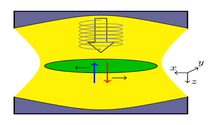
Figure 1: Schematic illustration of a quantum spin Hall insulator with spin filtered edge state placed inside an optical cavity. The green ellipse-like object represents the quantum spin Hall insulator that supports the edge states, while the blue and red arrows the spin-momentum locked electrons on the edge. The wave vector of the cavity mode is perpendicular to the direction of the edge electrons.

Let us first discuss the case when $g_{A}=0$, which makes Eq. (1) an inhomogeneous Dicke modelinhom . Without $g_{A}$ the Hamiltonian exhibits U(1) symmetry, indeed $e^{i\phi(a^{\dagger}a+\sum_{p}S_{p}^{z})}$ leaves the Hamiltonian invariant and the total number of excitations $N=a^{\dagger}a+\sum_{p}S_{p}^{z}$ is a constant of motion. Time reversal is the other symmetry of the system without $g_{A}$, using $\mathcal{T}=e^{i\pi(a^{\dagger}a+\sum_{p}S_{p}^{y})}\mathcal{K}$, where $\mathcal{K}$ is complex conjugation, the Hamiltonian is unchanged:

$$\mathcal{T}(a,a^{\dagger},p,S_{p}^{\pm},S_{p}^{z})\mathcal{T}^{-1}=(-a,-a^{\dagger},-p,-S_{p}^{\pm},-S_{p}^{z}).$$

Reintroducing $g_{A}$ destroys the U(1) symmetry which means that the total number of excitations are no longer conserved. Since $\mathcal{T}$ leaves the vector potential term invariant, the sole symmetry of the full system is time reversal. Furthermore, the system is integrable when U(1) symmetry is present and its mean field solution coincides with the exact solutioneastlittle . One can argue that if we integrate out the photon degree of freedom, the resulting effective electron-electron interaction has the form $-\tilde{g}L^{-1}\sum_{p,p^{\prime}}S^{+}_{p}S^{-}_{p^{\prime}}$ which describes an infinite range and constant strength interaction that makes the mean field results in the thermodynamic limit ($L\to\infty$) exact. The same argument holds when $g_{A}\neq 0$. After integrating out the photon field it yields an effective interaction:

$$H_{eff}=-\frac{\tilde{g}}{L}\sum_{p,p^{\prime}}S^{+}_{p}S^{-}_{p^{\prime}}$$

$$-\frac{\sqrt{\tilde{g}\tilde{g_{A}}}}{\omega L}\sum_{p,p^{\prime}}\left(S^{+}_{p}S^{z}_{p^{\prime}}+S^{z}_{p}S^{-}_{p^{\prime}}\right)-\frac{\tilde{g_{A}}}{\omega^{3}L}\sum_{p,p^{\prime}}S_{p}^{z}S_{p^{\prime}}^{z},$$ (2)

which also describes infinite range and constant strength interactions between electrons, therefore the mean field solution in the thermodynamic limit is still exact. The last term in Eq. (2) is a ferromagnetic coupling between electron spins mediated by the vector potential of the cavity field, as we will see this results in a generated photocurrent along the edges.

II.1 Mean field theory

In the thermodynamic limit the photon field becomes macroscopically occupiedemaryprl : $\langle a\rangle=\sqrt{nL}e^{i\varphi}$, the system is in a superradiant phase. The mean field description means that we replace the bosonic operators with their mean value and then the Hamiltionian in Eq. (1) becomes:

$$H_{MF}=\omega nL+\sum_{p}\begin{pmatrix}c^{\dagger}_{p\uparrow}&c^{\dagger}_{p\downarrow}\end{pmatrix}\begin{pmatrix}\varepsilon_{p}&\Delta\\ \Delta^{*}&-\varepsilon_{p}\end{pmatrix}\begin{pmatrix}c_{p\uparrow}\\ c_{p\downarrow}\end{pmatrix},$$ (3)

where $\varepsilon_{p}=vp+g_{A}\sqrt{n}\cos\varphi$ and $\Delta=g\sqrt{n}e^{i\varphi}$. Eq. (3) is easily diagonalized by the Bogoliubov transformation:

$$\begin{pmatrix}c_{p\uparrow}\\ c_{p\downarrow}\end{pmatrix}=\begin{pmatrix}\cos\vartheta&e^{i\varphi}\sin\vartheta\\ -e^{-i\varphi}\sin\vartheta&\cos\vartheta\end{pmatrix}\begin{pmatrix}d_{p+}\\ d_{p-}\end{pmatrix},$$ (4)

where $\tan 2\vartheta=-|\Delta|/\varepsilon_{p}$ and Eq. (3) becomes:

$$H_{MF}=\omega nL+\sum_{p,\alpha}E_{\alpha}(p)d^{\dagger}_{p\alpha}d_{p\alpha}.$$ (5)

Here, $\alpha=\pm 1$ and $E_{\alpha}(p)=\alpha E_{p}$ with:

$$E_{p}=\sqrt{(vp+g_{A}\sqrt{n}\cos\varphi)^{2}+g^{2}n}.$$ (6)

The mean field parameters $(n,\varphi)$ which are understood as the mean photon number density and the phase of the order parameter, respectively, can be calculated by minimizing the total ground-state energy $(E_{gs})$. At half filling the $\alpha=-1$ band is fully populated and the ground-state energy with $W$ cutoff energy and $\rho=1/v\pi$ 1D density of states is:

$$\frac{E_{gs}}{L}=\omega n-\frac{1}{L}\sum_{p}\sqrt{\varepsilon_{p}^{2}+|\Delta|^{2}}=$$ (7)

$$-\frac{\rho W^{2}}{2}+\left(\omega-\frac{\rho g_{A}^{2}}{2}\cos^{2}\varphi\right)n-\frac{\rho|\Delta|^{2}}{4}\left(1+\ln\frac{4W^{2}}{|\Delta|^{2}}\right)$$

With $g_{A}=0$ the energy exhibits a mexican hat structure in the Re$\langle a\rangle-$Im$\langle a\rangle$ space, see Fig. 2., the phase remains undetermined and the ground-state is infinitely degenerate due to U(1) symmetry. When $g_{A}\neq 0$ the mexican hat structure developes two minima along Re$\langle a\rangle$ and the minimum energy appears when $\cos^{2}\varphi=1$. The ground-state is now doubly degenerate due to time reversal symmetry which is spontaneously broken in the emerging superradiant phase.

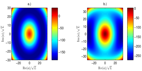
Figure 2: The contourplot for the total ground-state energy. In panel a.) $g_{A}=0$, the energy exhibits a mexican hat structure with $\varphi\in[0,2\pi]$ one can sweep through the ground-state manifold with no energy cost. In panel b.) $\rho g_{A}=0.1$ the minimum bends toward the real axis when $\varphi=0$ and $\pi$, so tunneling between the two degenerate ground-state will require a finite amount of energy. The other parameters used: $\rho W=100$, $\rho\omega=1$, $\rho g=1$.

By carrying out the minimalization of Eq. (7) we find the phase and mean photon number density to be:

$$\varphi=m\pi,\quad m\in\mathbb{Z}\quad\quad\quad$$

$$n=\frac{4W^{2}}{g^{2}}\exp\left(\frac{2\rho g_{A}^{2}-4\omega}{\rho g^{2}}\right).$$ (8)

The mean photon number density as the function of the Zeeman coupling $g$ is always strictly positive: $n(g)>0$. Since we assume the vector potential coupling strength is always smaller than the Zeeman coupling ($g>g_{A}$), the photon number density has a maxima at $\rho g_{max}=\sqrt{4\rho\omega-2\rho^{2}g_{A}^{2}}$ with $n_{max}=2\rho W^{2}\exp(-1)/(2\omega-\rho g_{A}^{2})$, see Fig. 3. Detecting the photon number can be achieved by various quantum nondemolition measurementsfdet1 ; fdet2 , for example subjecting the field to a quasiresonant beam of Rydberg atoms and measuring the resulting phase shift of the atomic wave functionfotondet .

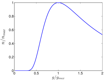
Figure 3: The mean photon number density as the function of the Zeeman coupling. The parameters used: $\rho\omega=1$, $\rho g_{A}=0.1$.

The conventional Dicke model of two level atoms predicts a phase transition at a critical coupling constantemarybrandes . On the other hand, considering the effects of the vector potential as a diamagnetic term, it can be shown that the condition for a stable superradiant phase is never satisfied due to the Thomas–Reiche–Kuhn sum rule for atomic systemsnogo ; unstab ; polini . This is known as a no-go theorem. The main differences between our model and the conventional Dicke model is that the edge electrons have linear dispersion while the Dicke two level atoms have a constant energy difference between levels and the fact that here the vector potential appears as a linear term while the diamagnetic term is quadratic. The Dicke critical coupling constant is proportional to the square root of the energy difference between the atomic levels, for linearly dispersive two level systems this critical value reduces to zero. Eq. (8) shows us that for arbitrary small $g>0$ and for every $g_{A}$ the photon states are macroscopically occupied: $\langle a^{\dagger}a\rangle=nL$, thus our system is always in its superradiant phase as nothing prevents the phase transition from occuring.

II.1.1 Properties of the ground-state

In the emerging superradiant ground-state time reversal symmetry is spontaneously broken. This fact is proven by the magnetic properties of this state. Indeed using the Bogoliubov transformation, we get the spin expectation values as

$$\langle S^{x}\rangle=\frac{1}{L}\sum_{p}\langle S_{p}^{x}\rangle=-\frac{1}{2L}\sum_{p}\frac{|\Delta|\cos\varphi}{\sqrt{\varepsilon_{p}^{2}+|\Delta|^{2}}},$$

$$\langle S^{y}\rangle=\frac{1}{L}\sum_{p}\langle S_{p}^{y}\rangle=\frac{1}{2L}\sum_{p}\frac{|\Delta|\sin\varphi}{\sqrt{\varepsilon_{p}^{2}+|\Delta|^{2}}},$$ (9)

$$\langle S^{z}\rangle=\frac{1}{L}\sum_{p}\langle S_{p}^{z}\rangle=-\frac{1}{2L}\sum_{p}\frac{\varepsilon_{p}}{\sqrt{\varepsilon_{p}^{2}+|\Delta|^{2}}}.$$

The magnetization along the $x$ and $z$ axis are nonzero and their measured value would determine $\varphi$. The calculations show us that the magnetization is proportional to the gap $|\Delta|$:

$$\langle S^{x}\rangle=-\frac{\rho}{2}|\Delta|\ln\frac{2W}{|\Delta|}\cos\varphi,$$

$$\langle S^{y}\rangle=0,$$ (10)

$$\langle S^{z}\rangle=-\rho|\Delta|\frac{g_{A}}{2g}\cos\varphi.$$

The finite $\langle S^{z}\rangle$ also means that a net photocurrent is generated along the edge through the magnetoelectric effectsajat . Using the edge Hamiltonian $H=\sum_{p}2vpS_{p}^{z}$ and introducing a vector potential $A$ to the momentum as an external drive, we can determine by varying $H$ with respect to $A$ that the current density operator is:

$$j(q)=\sum_{p,q}ev(c^{\dagger}_{p+q\uparrow}c_{p\uparrow}-c^{\dagger}_{p+q\downarrow}c_{p\downarrow})e^{-iqr}.$$ (11)

The current operator for $q=0$ is $j=2ev\sum_{p}S_{p}^{z}$, hence:

$$\langle j\rangle=2ev\langle S^{z}\rangle=-ev\rho|\Delta|\frac{g_{A}}{g}\cos\varphi.$$ (12)

The photocurrent is zero when $g_{A}=0$ which means that the vector potential generates it. This follows from the fact that in Eq. (1) the vector potential term is similar to an effective magnetic field. Furthermore, we showed earlier that after integrating out the photon field it yields us a vector potential mediated ferromagnetic coupling between spins, which leads to nonzero expectation value for the magnetization . The direction of the photocurrent is determined by the phase $\varphi$, with $\cos\varphi~{}=~{}(-1)^{m}$.

III Photon Field

After detailing the effects of the cavity on the material, now we turn to the photon field and how it changes due to the interaction with the edge electrons. To this end, we will study the fluctuations over the mean field parameters which conveniently reveals the validity range of the mean field resultseastham . We previously presented a physical argument for this, as the effective interactions between electrons have infinite range the mean field results must be exact. Now we make a quantitative argument as well. Following Ref.[eastham, ] and making use of coherent state path integral formalism we introduce $\phi$ as a complex field for the photons and $\psi_{p\sigma}$ Grassmann fields for the edge electrons. The partition function can be computed as

$$Z=\text{Tr}e^{-\beta H}=\int\mathcal{D}\phi\int\mathcal{D}\psi\text{ }e^{-S}$$ (13)

with action

$$S=\int_{0}^{\beta}d\tau\bar{\phi}(\partial_{\tau}+\omega)\phi+\sum_{p}\bar{\eta}_{p}M_{p}\eta_{p}=S_{ph}+S_{el}$$

where $\bar{\eta}_{p}=\left(\bar{\psi}_{p\uparrow}\text{ }\bar{\psi}_{p\downarrow}\right)$ is a spinor and the matrix

$$M_{p}=\begin{pmatrix}\partial_{\tau}+vp+\frac{g_{A}}{\sqrt{L}}\text{Re}\phi&\frac{g}{\sqrt{L}}\phi\\ \frac{g}{\sqrt{L}}\bar{\phi}&\partial_{\tau}-vp-\frac{g_{A}}{\sqrt{L}}\text{Re}\phi\end{pmatrix}.$$

Because of superradiance we rescale the photon field $\phi\to\sqrt{L}\phi$ and integrate out the electron fields. The partition function becomes

$$Z=\int\mathcal{D}\phi\int\mathcal{D}\psi\text{ }e^{-S}=\int\mathcal{D}\phi\text{ }e^{-LS_{eff}}$$ (14)

with effective action

$$S_{eff}=\int_{0}^{\beta}d\tau\bar{\phi}(\partial_{\tau}+\omega)\phi-\frac{1}{L}\ln\left(\int\mathcal{D}\psi\text{ }e^{-S_{el}}\right).$$ (15)

If we proceed and try to find the minima of this action ($S_{0}$) with $\delta S_{eff}/\delta\bar{\phi}=0$ we arrive at the mean field results Eq. (8) as $\phi=\sqrt{n}e^{i\varphi}$. The next step is expanding the effective action around the mean field results to second order which is equivalent to studying the fluctuations around the mean field parameters: $S_{eff}=S_{0}+S_{2}(\delta\bar{\phi},\delta\phi)$. With this expansion the partition function becomes

$$Z=\int\mathcal{D}\phi\text{ }e^{-LS_{eff}}=e^{-LS_{0}}\int\mathcal{D}\phi\text{ }e^{-LS_{2}}.$$ (16)

Here the $e^{-LS_{O}}$ term contributes to the mean field result for the free energy. The remaining functional integral gives us the second order correction to the free energy:

$$F\propto\ln Z=F_{MF}+\frac{1}{L}\ln\det\mathcal{D}^{-1},$$ (17)

where $\mathcal{D}^{-1}$ is the inverse of the Green’s function of the photons. It appears because it is the kernel of the action correction $S_{2}$ and the determinant appears because the functional integral has a simple Gaussian integral form. Since the mean field parameters minimize the effective action this means that $\det\mathcal{D}^{-1}$ should be positive. In the thermodynamic limit ($L\to\infty$) the correction vanishes thus making the mean field results exact and the superradiant phase as the ground state stable. We will see that $\mathcal{D}^{-1}$ has zero eigenvalues which describe the Goldstone modes of this systemgoldhiggs , however these modes do not contribute to the free energy in the thermodynamic limit.

III.1 Green’s function of the photons

Instead of calculating the kernel of the second order correction to the effective action, we construct the photon Green’s function with diagram technique. Introducing the fluctuations over the mean field parameters we modify Eq. (3) with $a\to\langle a\rangle+a$:

$$H=\omega a^{\dagger}a+\sum_{p}\begin{pmatrix}c^{\dagger}_{p\uparrow}&c^{\dagger}_{p\downarrow}\end{pmatrix}\begin{pmatrix}\varepsilon_{p}&\Delta\\ \Delta^{*}&-\varepsilon_{p}\end{pmatrix}\begin{pmatrix}c_{p\uparrow}\\ c_{p\downarrow}\end{pmatrix}$$

$$+\frac{g_{A}}{\sqrt{L}}\sum_{p}\left(a+a^{\dagger}\right)S_{p}^{z}+\frac{g}{\sqrt{L}}\sum_{p}\left(aS_{p}^{+}+a^{\dagger}S_{p}^{-}\right)$$ (18)

where the first row is the unperturbed mean field Hamiltonian and the second row is understood as the perturbation. In the Nambu space $\left(a\text{ }a^{\dagger}\right)$ the photon Green’s function is

$$\mathcal{D}(\tau)=-\left\langle T_{\tau}\begin{pmatrix}a(\tau)a^{\dagger}(0)&&a^{\dagger}(\tau)a^{\dagger}(0)\\ a(\tau)a(0)&&a^{\dagger}(\tau)a(0)\end{pmatrix}\right\rangle.$$ (19)

The appearance of anomalous terms are evident from the perturbation as it contains single creation and annihilation photon operators. Because of this, first order diagrams have no contribution and the first non vanishing terms come from second order diagrams, which are single fermion loops.

Evaluating these loops in Matsubara frequency space using Dyson’s equation we arrive at the inverse Green’s function for the photons:

$$\mathcal{D}^{-1}(i\omega_{n})=\mathcal{D}^{-1}_{0}(i\omega_{n})-\Sigma=\begin{pmatrix}K_{1}&&K_{2}\\ K_{2}^{*}&&K_{1}^{*}\end{pmatrix},$$

$$K_{1}=i\omega_{n}-\omega+\frac{1}{L}\sum_{p}\Bigg{[}\frac{4g_{A}^{2}|\Delta|^{2}+g^{2}(i\omega_{n}\varepsilon_{p}+\varepsilon_{p}^{2}+E_{p}^{2})}{E_{p}(4E_{p}^{2}+\omega_{n}^{2})}$$

$$-\frac{2gg_{A}|\Delta|(2\varepsilon_{p}-i\omega_{n})}{E_{p}(4E_{p}^{2}+\omega_{n}^{2})}\Bigg{]}\tanh\left(\frac{\beta E_{p}}{2}\right),$$

$$K_{2}=\frac{1}{L}\sum_{p}\frac{4g_{A}^{2}|\Delta|^{2}-g^{2}\Delta^{2}-2gg_{A}\Delta\varepsilon_{p}}{E_{p}(4E_{p}^{2}+\omega_{n}^{2})}\tanh\left(\frac{\beta E_{p}}{2}\right).$$

Since we are interested in the properties of the ground state of this system we make the $T\to 0$ limit and obtain the retarded Green’s function as the analytic continuation of Eq. (III.1).

III.2 Photon spectral function

The spectral function, defined as the complex part of the trace of the retarded Green’s function, is:

$$A(\Omega)=-\frac{1}{\pi}\text{ImTr}\mathcal{D}(\Omega).$$ (21)

Carrying out the analytic continuation of Eq. (III.1) ($i\omega_{n}~{}\to~{}\Omega~{}+~{}i\eta$, with $\eta=0^{+}$) yields us the following integrals:

$$\frac{1}{L}\sum_{p}\frac{-4|\Delta|^{2}}{E_{p}((\Omega+i\eta)^{2}-4E_{p}^{2})}=\rho f_{0}(\Omega),$$

$$\frac{1}{L}\sum_{p}\frac{\varepsilon_{p}}{E_{p}((\Omega+i\eta)^{2}-4E_{p}^{2})}=0,$$ (22)

$$\frac{1}{L}\sum_{p}\frac{\varepsilon_{p}^{2}}{E_{p}((\Omega+i\eta)^{2}-4E_{p}^{2})}=\displaystyle{\frac{\rho}{4}f_{2}(\Omega)-\frac{\omega}{2g^{2}}+\frac{\rho g_{A}^{2}}{4g^{2}}}.$$

The complete forms of $f_{0}$ and $f_{2}$ are given in the Appendix. The properties of these complex valued functions reveal information about the nature of the photon spectral function in Eq. (21). The real parts of $f_{0}$ and $f_{2}$ go to unity when $\Omega$ tends to zero: $\lim_{\Omega\to 0}f_{0,2}(\Omega)=1$. Furthermore, they have vanishing imaginary part when $\Omega<2|\Delta|$ and this sets the threshold energy for continuum polariton excitations for $\Omega>2|\Delta|$. Indeed, using the integrals in Eq. (22) the resulting spectral function is zero for frequencies below $2|\Delta|$, except for a well defined $\Omega_{0}$ value:

$$A(\Omega<2|\Delta|)\propto\text{Im}(F(\Omega)-i\eta)^{-1}=\pi|F^{\prime}(\Omega_{0})|^{-1}\delta(\Omega-\Omega_{0}).$$

Here $\Omega_{0}$ is the real root of the function $F(\Omega)$ defined as:

$$F(\Omega)=\left(\frac{\rho g_{A}^{2}}{2}-\rho g_{A}^{2}f_{0}(\Omega)+\frac{\rho g^{2}}{2}f_{2}(\Omega)-\frac{\rho g^{2}}{4}f_{0}(\Omega)\right)^{2}$$

$$-\left(\rho g_{A}^{2}f_{0}(\Omega)-\frac{\rho g^{2}}{4}f_{0}(\Omega)\right)^{2}-\Omega^{2}\left(1-\frac{\rho gg_{A}}{2|\Delta|}f_{0}(\Omega)\right)^{2}.$$

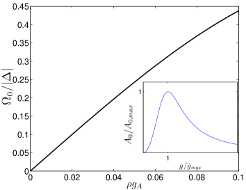
Figure 4: The real root of $F(\Omega_{0})=0$ as the function of increasing vector potential coupling strength ($g_{A}$). This is understood as the energy requirement for phase fluctuations and as the energy of the gapped Goldstone mode. The parameters used: $\rho\omega=1$, $\rho g=0.4$. The inset figure is the spectral weight of the Goldstone mode as the function of the Zeeman coupling with parameters: $\rho W=100$, $\rho\omega=1$.

Taking $g_{A}\to 0$ in $F(\Omega)$ results in $\Omega_{0}=0$. When $g_{A}=0$ the ground state is infinitely degenerate as seen in Fig 2. due to U(1) symmetry and one can sweep through this ground state manifold with no energy cost. This gives rise to a zero energy Goldstone mode which is understood as the phase fluctuation of the superradiant condensate and this appears in the spectral function:

$$A(\Omega<2|\Delta|)=\frac{6\rho g^{2}|\Delta|^{2}}{12|\Delta|^{2}+(\rho g^{2})^{2}}\delta^{\prime}(\Omega)=A_{0}\delta^{\prime}(\Omega).$$ (24)

The spectral weight of the Goldstone mode vanishes with $g$. Since the gap depends on $g$ according to Eq. (8) it has a maxima ($A_{0,max}$) at the solution of $\ln\frac{48W^{2}}{x(x-\omega)}=\frac{4\omega}{x}$ for $x=\rho\hat{g}_{max}^{2}$ and vanishes as $g$ increases. This is shown in the inset of Fig. 4. In the presence of a nonzero $g_{A}$ phase fluctuations will require finite amount of energy, thus making the Goldstone mode gapped which is described in $\Omega_{0}$, see Fig 4.

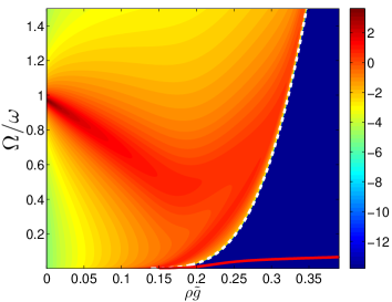
Figure 5: The contour plot of the spectral function $\ln(\omega A(\Omega))$ as the function of the Zeeman coupling $\rho\tilde{g}$ with $g_{A}=0.1$. The energy of the Goldstone mode $\Omega_{0}$ is shown as the red solid line in the $\Omega<2|\Delta|$ regime. The white dashed line denotes the minimum excitation energy $2|\Delta|$, above which the polariton continuum is formed. The parameters used: $\rho W=100$, $\rho\omega=1$.

In the $\Omega>2|\Delta|$ case the complex part of the functions $f_{0}$ and $f_{2}$ are nonzero and we get the polariton excitations and their spectral weight in the spectral function $A(\Omega>2|\Delta|)$, which is measurable by the absorption coefficient of the cavity. Without interactions the spectral function has the form $A(\Omega)=\delta(\Omega-\omega)$ with the bare $\omega$ cavity mode. On Fig. 5. it is noticable that this mode is shifted down from $\omega$ because of $g_{A}$ and with increasing $g$ it gets damped as $\sim\rho g^{2}$. Eventually it renormalizes into smaller frequencies before hitting the optical gap at $\Omega=2|\Delta|$, where the spectral function exhibits a square root singularity. Apart from shifting $\omega$ for small $g$ the vector potential coupling does not have significant contribution to the nature of the polariton continuum.

IV Conductivity along the edge

Equipped with the photon Green’s function, we can evaluate the Kubo formula for the frequency dependent optical conductivity along the edge. The density-density correlation function, which is readily related to the optical conductivity, can be investigated by shot noise measurements. In addition, the optical conductivity can directly be probed by the amplitude or phase modulation of the optical latticeoptcond ; optcond1 , that realizes the spin Hall insulator of our system.

The response for an external drive have two contributions:

$$\sigma=\sigma_{Kubo}+\sigma_{dia}.$$ (25)

The first is the direct result for the conductivity computed from the Kubo formula:

$$\sigma_{Kubo}=\frac{\chi(\Omega)}{i\Omega},$$ (26)

where $\chi$ is the current-current correlation function.

$$\chi(\tau)=\langle T_{\tau}j(\tau)j(0)\rangle=4e^{2}v^{2}\sum_{p}\langle T_{\tau}S_{p}^{z}(\tau)S_{p}^{z}(0)\rangle.$$ (27)

The second term in Eq. (25) is a diamagnetic term. By diagonalising the Hamiltonian in the presence of an external vector potential, the resulting spinor wavefunctions will depend on the vector potential through the Peierls substitution. Calculating the expectation value of the current operator to first order in the vector potential gives us the diamagnetic contribution in the conductivity formula: $\sigma_{dia}=-\rho e^{2}v^{2}/(i\Omega)$. This is akin to the origin of a diamagnetic term in graphene where the energy dispersion is also lineargeimgraf ; condgraf .

We calculate the correlation function in Eq. (27) diagramatically in Matsubara frequency space. The diagrams we need to consider are a single fermion loop and a collective mode diagramlee . Evaluation of the single fermion loop gives us:

$$\Pi_{zz}^{0}(i\omega_{n})=-\frac{T}{L}\sum_{p,\nu_{n}}\text{Tr}[\sigma^{z}\mathcal{G}(i\nu_{n})\sigma^{z}\mathcal{G}(i\nu_{m}-i\omega_{n})].\text{ }$$ (28)

Here $\mathcal{G}$ is the electron Green’s function, using Eq. (4) and Eq. (5) this reads as:

$$\mathcal{G}(p,i\nu_{n})=\frac{1}{(i\nu_{n})^{2}-E_{p}^{2}}\begin{pmatrix}i\nu_{n}+\varepsilon_{p}&&\Delta\\ \Delta^{*}&&i\nu_{n}-\varepsilon_{p}\end{pmatrix}.$$ (29)

The term $\Pi_{zz}$ is related to the correlation function in Eq. (27) as $\chi=v^{2}\Pi$. Summing over the frequencies and momenta in Eq. (28) and taking the temperature to zero, we get:

$$\Pi_{zz}^{0}(\Omega)=\rho f_{0}(\Omega).$$ (30)

To evaluate the collective diagram we need to construct the RPA equations. Instead of using $\mathcal{D}_{0}$ the unperturbed photon propagator and consider a connected RPA system of equations, we follow here a different approach. Since we already calculated the full photon propagator in Eq. (III.1), we sum up all the possible combinations that would appear from the interaction term of Eq. (III.1). This immediately gives us the correlation function:

$$\Pi_{zz}=\Pi_{zz}^{0}-g^{2}\left(\Pi_{z+}^{0}\mathcal{D}_{aa}\Pi_{+z}^{0}+\Pi_{z+}^{0}\mathcal{D}_{aa^{\dagger}}\Pi_{-z}^{0}+\Pi_{z-}^{0}\mathcal{D}_{a^{\dagger}a}\Pi_{+z}^{0}+\Pi_{z-}^{0}\mathcal{D}_{a^{\dagger}a^{\dagger}}\Pi_{-z}^{0}\right)$$

$$-g_{A}^{2}\left(\Pi_{zz}^{0}\mathcal{D}_{aa}\Pi_{zz}^{0}+\Pi_{zz}^{0}\mathcal{D}_{aa^{\dagger}}\Pi_{zz}^{0}+\Pi_{zz}^{0}\mathcal{D}_{a^{\dagger}a}\Pi_{zz}^{0}+\Pi_{zz}^{0}\mathcal{D}_{a^{\dagger}a^{\dagger}}\Pi_{zz}^{0}\right)$$

$$-gg_{A}\left(\Pi_{z+}^{0}\mathcal{D}_{aa}\Pi_{zz}^{0}+\Pi_{z+}^{0}\mathcal{D}_{aa^{\dagger}}\Pi_{zz}^{0}+\Pi_{z-}^{0}\mathcal{D}_{a^{\dagger}a}\Pi_{zz}^{0}+\Pi_{z-}^{0}\mathcal{D}_{a^{\dagger}a^{\dagger}}\Pi_{zz}^{0}\right)$$

$$-g_{A}g\left(\Pi_{zz}^{0}\mathcal{D}_{aa}\Pi_{+z}^{0}+\Pi_{zz}^{0}\mathcal{D}_{aa^{\dagger}}\Pi_{-z}^{0}+\Pi_{zz}^{0}\mathcal{D}_{a^{\dagger}a}\Pi_{+z}^{0}+\Pi_{zz}^{0}\mathcal{D}_{a^{\dagger}a^{\dagger}}\Pi_{-z}^{0}\right).$$ (31)

The minus signs in front of the couplings come from the definition of the photon propagator in Eq. (19). In Eq. (31) there are four more frequency sums:

$$\Pi_{ab}^{0}(i\omega_{n})=-\frac{T}{L}\sum_{p,\nu_{n}}\text{Tr}[\sigma^{a}\mathcal{G}(i\nu_{n})\sigma^{b}\mathcal{G}(i\nu_{m}-i\omega_{n})],$$

with $a$ and $b$ are $z$ or $\pm$. Doing the same procedure as in Eq. (28) these cross correlations are:

$$\Pi_{\pm z}^{0}(\Omega)=\mp\Pi_{z\mp}^{0}(\Omega)=\pm\frac{\rho\Omega}{4|\Delta|}f_{0}(\Omega).$$

To summarize Eq. (31) we gather every term into a single function:

$$\Pi_{zz}(\Omega)=\rho\left[f_{0}(\Omega)-C(\Omega)f_{0}(\Omega)\right],$$ (32)

and we arrive at the full optical conductivity formula:

$$\sigma(\Omega)=\frac{\rho e^{2}v^{2}}{i\Omega}\left[f_{0}(\Omega)-1-C(\Omega)f_{0}(\Omega)\right].$$ (33)

This expression is very similar to other conductivity formulas for electron-phonon coupled systems calculated with RPAvirobacsi ; vanyolos2 .

Let us first examine the properties of the conductivity through the function $C$ when $g_{A}=0$. In this case we need to condsider the first row of Eq. (31), the function $C$ has the form:

$$C(\Omega)=-\frac{\Omega^{2}}{4|\Delta|^{2}}\frac{f_{0}(\Omega)f_{2}(\Omega)}{f_{2}(\Omega)(f_{2}(\Omega)-f_{0}(\Omega))-\frac{4}{\rho^{2}g^{4}}\Omega^{2}-i\eta}.$$

When $\Omega\to 0$, $C(0)=\rho^{2}g^{4}/(\rho^{2}g^{4}+16|\Delta|^{2})$. By the Kramers–Kronig relation, this implies a Dirac delta function at the origin of the real part of the conductivity. Indeed making the $\eta\to 0^{+}$ limit we get the Dirac delta in accordance with Kramers–Kronig. This result clearly comes from the full photon propagator and is absent from the single particle contribution to the optical response, therefore the Goldstone mode manifests itself in the conductivity formula as a Drude peak:

$$\sigma_{Goldstone}=\pi\rho e^{2}v^{2}\frac{\rho^{2}g^{4}}{\rho^{2}g^{4}+16|\Delta|^{2}}\delta(\Omega).$$ (34)

If we take the $g\to 0$ then $\sigma_{Goldstone}=\pi\rho e^{2}v^{2}\delta(\Omega)$, so it becomes the conventional Drude weightdrude . This allows us to introduce an effective mass due to light-matter interaction. The Drude weight of the non-interacting system reads as $n_{e}e^{2}/m$, where $n_{e}$ is the particle number density of the edge electrons and $m$ is their mass. In the presence of interaction, we rewrite the Goldstone conductivity as

$$\sigma_{Goldstone}=\frac{\pi n_{e}e^{2}}{m^{*}}\delta(\Omega),$$ (35)

with effective mass:

$$\frac{m}{m^{*}}=\frac{\rho^{2}g^{4}}{\rho^{2}g^{4}+16|\Delta|^{2}}.$$ (36)

The $C$ function is a combination of the previously defined $f_{0,2}$ functions, which indicates that the real part of the conductivity must be zero for frequencies below $2|\Delta|$. The behaviour of Re$(\sigma)$ is shown in Fig. 6., with $C=0$ the single particle term has a square root singularity at frequency twice the gap. Considering the collective modes the square root singularity still remains, however a portion of the weight of the conductivity is transferred into the weight of the Goldstone mode, so that the conductivity sum rule is not violated, indeed:

$$\int_{0}^{\infty}\text{d}\Omega\text{ Re}(\sigma(\Omega))=\frac{\pi}{2}\rho e^{2}v^{2}.$$ (37)

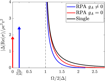
Figure 6: The frequency dependent conductivity of the edges. The solid black is the single particle result, the red contains the collective terms with $\rho g_{A}=0$ and the blue contains all terms with $\rho g_{A}=0.1$. The Goldstone peaks are also depicted, as $g_{A}$ is nonzero the peak moves to frequency $\Omega_{0}$ and its weight increases. Further parameters: $\rho\omega=1,\rho W=100,\rho g=0.4$.

Turning now to the case when $g_{A}$ is nonzero the function $C$ is given by Eq. (31). Notice that in Eq. (27) for convenience we used a time ordered product instead of a commutator in the Kubo formula. Unless the current operator possess a nonzero expectation valueelectronliquid , these two approaches give the same result. However, in Eq. (12), the current operator has a finite expectation value in the ground-state, which means that our result contains an extra term in Eq. (31), which is only present in the time ordered product but should be absent from the commutator:

$$-\frac{\rho^{2}g_{A}^{4}f_{0}(\Omega)}{F(\Omega)-i\eta}.$$ (38)

This we must neglectelectronliquid . The correct expression, in accordance with the linear response commutator from the Kubo formula, is:

$$C(g_{A},\Omega)=-\frac{\rho f_{0}(\Omega)}{F(\Omega)-i\eta}\Big{[}\frac{g^{2}\Omega^{2}}{16|\Delta|^{2}}\big{(}\rho g_{A}^{2}-4\rho g_{A}^{2}f_{0}(\Omega)$$

$$+\rho g^{2}f_{2}(\Omega)\big{)}+\rho g_{A}^{2}g^{2}(f_{2}(\Omega)-f_{0}(\Omega))$$

$$+\frac{gg_{A}\Omega^{2}}{|\Delta|}\left(1-\frac{\rho gg_{A}}{2|\Delta|}f_{0}(\Omega)\right)\Big{]}.$$ (39)

When $\Omega\to 0$ Eq. (39) vanishes and thus the Drude peak disappears. However, the real part of the conductivity still has a Dirac delta at the frequency where $F(\Omega)=0$, which corresponds to the gapped Goldstone mode energy $\Omega_{0}$:

$$\sigma_{Goldstone}=\frac{\pi n_{e}e^{2}}{m^{*}}\delta(\Omega-\Omega_{0}),$$ (40)

with effective mass that depends on the energy of the gapped Goldstone mode:

$$\frac{m}{m^{*}}=\frac{\Omega_{0}f_{0}(\Omega_{0})^{2}}{16|\Delta|^{2}|F^{\prime}(\Omega_{0})|}\bigg{[}\rho^{2}g^{4}f_{2}(\Omega_{0})+16\rho gg_{A}|\Delta|$$

$$+\rho^{2}g^{2}g_{A}^{2}\big{(}1-16f_{0}(\Omega_{0}))\big{)}\bigg{]}.$$ (41)

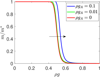
Figure 7: The effective mass as the function of the Zeeman interaction strength is plotted and it resembles a step function. The arrow indicates that the increase of $g_{A}$ shifts this step, thus the effective mass becomes infinite at larger Zeeman coupling strength. This means that the interaction involving the vector potential is making the collective modes more stable at larger $g$. The parameters used: $\rho\omega=1,\rho W=100.$

Instead of a dc conductivity we get a low frequency ac one at $\Omega_{0}$. These results are very similar to the interband conductivity obtained when studying electron interaction with Fröhlich phonons, there the resulting dc conductivity becomes a low frequency ac due to Coulomb interactionslee .

In the absence of interactions, the real part of the conductivity of the edge electrons consists of only the bare Drude peak with mass $m$. As the Zeeman interaction appears the weight of this Drude peak decreases ($m^{*}$ increases) and the real part of the conductivity is now nonzero for frequencies over $2|\Delta|$. As $g$ grows so does the effective mass and when the coupling strength $g$ is comparable with the photon frequency ($g\approx\omega$) the effective mass renormalizes to nearly infinity, see Fig. 7, thus making the collective modes in the conductivity disappear. This means that the single particle description of the conductivity is sufficient in this parameter range. In addition to shifting the Drude peak to frequency $\Omega_{0}$, the appearance of $g_{A}$ also decreases the effective mass $m^{*}$. This can be seen on Fig. 6., as the conductivity curve when $g_{A}$ is nonzero is always under the curve of the zero $g_{A}$ case. The missing weight is transfered into the the weight of the Goldstone mode, due to the conductivity sum rule in Eq. (37), $m^{*}$ must decrease. This means that the vector potential interaction stabilizes the collective modes at stronger Zeeman couplings. Fig. 7. also supports this idea.

V Conclusion

Interaction between a circularly polarized quantum photon field and spin Hall edge electrons leads to a stable superradiant ground state at arbitrary Zeeman interaction strength. This ground state spontanously breaks time reversal symmetry and a net photocurrent or equivalently magnetization along axis-z through the magnetoelectric coupling, is generated by the vector potential part of the electromagnetic field. Above a threshold energy, corresponding to a Higgs mode, a continuum polariton excitations emerge from the single cavity mode and below the threshold a Goldstone mode arises from the phase fluctuations of the ground state. Without the coupling to the vector potential this mode sits at zero energy due to the broken continuous U(1) symmetry. The introduction of the vector potential decreases the symmetry of the system into discrete time reversal. This results in a gapped Goldstone mode as phase fluctuations require a finite amount of energy to connect the symmetry broken ground states. In an external classical electromagnetic field, this Goldstone mode manifests itself in the frequency dependent conductivity along the edges and produces a low frequency dc/ac conductivity, depending on the absence/presence of the vector potential term, respectively. When the Zeeman coupling becomes comparable with the photon frequency, these conductivity structures only survive if the interaction involving the vector potential is present. For larger frequencies, the conductivity is zero for frequencies smaller than twice the gap, and has a characteristic square root singularity at the Higgs mode, $\Omega=2|\Delta|$ and vanishes for increasing frequencies. Finally, we remark that the requirement for the observation of the superradiant phase that the temperature should be well below the gap size. Similarly to other predictions made by mean field theory, the transition temperature is always comparable to the gap sizebruus and as such for temperatures $T\ll\Delta$ the effects detailed above should be observable.

VI Appendix

VI.1 Derivation of the Hamiltonian in Eq. (1)

Our system involves spin-momentum locked edge electrons with linear momentum: $\varepsilon_{\sigma}(p)=\sigma vp,\,\sigma=\pm 1$ and $v$ is the Fermi velocity. With the definition of $c^{\dagger}_{p,\sigma}$ which creates an edge electron with momentum $p$ and spin $\sigma$, we have:

$$H_{edge}=\sum_{p,\sigma}\varepsilon_{\sigma}(p)c_{p\sigma}^{\dagger}c_{p\sigma}=\sum_{p}vp(c_{p\uparrow}^{\dagger}c_{p\uparrow}-c_{p\downarrow}^{\dagger}c_{p\downarrow}).$$ (42)

The edge electrons are placed inside a cavity (Fig. 1), that is having its own quantum dynamics. We are interested in the interaction of the edge electrons and a single mode of quantum light with fixed helicity. The energy of the mode is: $H_{field}=\omega a^{\dagger}a$, where $\omega$ and $a$ denote the frequency and annihilation operator of a photon with positive helicity, respectively. The interaction arises from the magnetic part of the electromagnetic field that interacts with the spin of an edge electron. This is a Zeeman interaction:

$$H_{Z}=\sum_{\alpha,\beta}\int\mathrm{d}^{3}r\,\Psi^{\dagger}_{\alpha}(\mathbf{r})\left(g_{e}\mu_{B}\mathbf{S}\cdot\mathbf{B}(\mathbf{r})\right)\Psi_{\beta}(\mathbf{r})$$

$$=\frac{g}{\sqrt{L}}\sum_{p}\left(aS_{p}^{+}+a^{\dagger}S_{p}^{-}\right).$$ (43)

Here $g=\frac{g_{e}\mu_{B}}{2c}\sqrt{\frac{\omega}{\varepsilon_{0}}}\equiv\sqrt{\tilde{g}\omega}$ is the coupling constant of the Zeeman term, we used:

$$\Psi_{\sigma}(\mathbf{r})=\frac{1}{\sqrt{L}}\sum_{p}c_{p\sigma}e^{ipr},$$

$$\mathbf{B}(\mathbf{r})=\frac{i}{c}\sqrt{\frac{\omega}{2\varepsilon_{0}L}}\left(\left(\mathbf{e}_{z}\times\mathbf{e}_{+}\right)ae^{ikr}-\left(\mathbf{e}_{z}\times\mathbf{e}_{+}^{*}\right)a^{\dagger}e^{-ikr}\right)$$

$$\mathbf{S}=\frac{1}{2}(\sigma^{x}\,\sigma^{y}\,\sigma^{z})^{T},\,\,S_{p}^{\pm}=\frac{1}{2}\sum_{\alpha,\beta}c^{\dagger}_{p,\alpha}\left(\sigma^{x}_{\alpha,\beta}\pm i\sigma^{y}_{\alpha,\beta}\right)c_{p,\beta}.$$ (44)

There is another interaction term present from the vector potential of the quantum electromagnetic field due to the Peierls substitution $(p\to p+eA)$:

$$H_{A}=\sum_{\alpha,\beta}\int\mathrm{d}^{3}r\,\Psi^{\dagger}_{\alpha}(\mathbf{r})\left(ev\sigma_{\alpha,\beta}^{z}A_{x}(\mathbf{r})\right)\Psi_{\beta}(\mathbf{r})$$

$$=\frac{g_{A}}{\sqrt{L}}\sum_{p}\left(a+a^{\dagger}\right)S_{p}^{z},$$ (45)

The final Hamiltonian in Eq. (1) is therefore:

$$H=H_{field}+H_{edge}+H_{A}+H_{Z}$$ (46)

VI.2 The complete forms of the functions $f_{0;2}$ in Eq. (22)

The functions $f_{0}$ and $f_{2}$ can be calculated from Eq. (22) with Eq. (6):

$$f_{0}(\Omega)=\frac{1}{\rho L}\sum_{p}\frac{-4|\Delta|^{2}}{E_{p}((\Omega+i\eta)^{2}-4E_{p}^{2})}=$$

$$-2v|\Delta|^{2}\int_{-W}^{W}\text{d}p\frac{1}{E_{p}((\Omega+i\eta)^{2}-4E_{p}^{2})}$$ (47)

and

$$f_{2}(\Omega)=\frac{2\omega}{\rho g^{2}}+\frac{g_{A}^{2}}{g^{2}}+\frac{1}{\rho L}\sum_{p}\frac{4\varepsilon_{p}^{2}}{E_{p}((\Omega+i\eta)^{2}-4E_{p}^{2})}=$$

$$\frac{2\omega}{\rho g^{2}}+\frac{g_{A}^{2}}{g^{2}}+2v\int_{-W}^{W}\text{d}p\frac{\varepsilon_{p}^{2}}{E_{p}((\Omega+i\eta)^{2}-4E_{p}^{2})}.$$ (48)

By carrying out the integration with respect to the momentum $p$ and disregard terms that is the order or lower than $W^{-1}$, we get the complete forms of $f_{0}$ and $f_{2}$ with $\Theta(x)$ Heaviside functions:

$$f_{0}(\Omega)=\frac{\Theta(2|\Delta|-\Omega)4|\Delta|^{2}}{\Omega\sqrt{4|\Delta|^{2}-\Omega^{2}}}\text{arctg}\frac{\Omega}{\sqrt{4|\Delta|^{2}-\Omega^{2}}}+\Theta(\Omega-2|\Delta|)\left[\frac{2i\pi|\Delta|^{2}}{\Omega\sqrt{\Omega^{2}-4|\Delta|^{2}}}-\frac{4|\Delta|^{2}}{\Omega\sqrt{\Omega^{2}-4|\Delta|^{2}}}\text{arth}\frac{\sqrt{\Omega^{2}-4|\Delta|^{2}}}{\Omega}\right]$$

$$f_{2}(\Omega)=\Theta(2|\Delta|-\Omega)\frac{\sqrt{4|\Delta|^{2}-\Omega^{2}}}{\Omega}\text{arctg}\frac{\Omega}{\sqrt{4|\Delta|^{2}-\Omega^{2}}}+\Theta(\Omega-2|\Delta|)\left[\frac{\sqrt{\Omega^{2}-4|\Delta|^{2}}}{\Omega}\text{arth}\frac{\sqrt{\Omega^{2}-4|\Delta|^{2}}}{\Omega}-\frac{i\pi\sqrt{\Omega^{2}-4|\Delta|^{2}}}{2\Omega}\right]$$

References

- (1) R. H. Dicke, Coherence in spontaneous radiation processes, Phys. Rev. 93, 99 (1954).
- (2) C. Emary and T. Brandes, Chaos and the quantum phase transition in the Dicke model, Phys. Rev. E 67, 066203 (2003).
- (3) K. Baumann, C. Guerlin, F. Brennecke, and T. Esslinger, Nature 464, 1301 (2010).
- (4) H. Keßler, J. Klinder, M. Wolke, and A. Hemmerich, Steering matter wave superradiance with an ultranarrow-band optical cavity, Phys. Rev. Lett. 113, 070404 (2014).
- (5) K. J. Arnold, M. P. Baden, and M. D. Barrett, Self-organization threshold scaling for thermal atoms coupled to a cavity, Phys. Rev. Lett. 109, 153002 (2012).
- (6) D. Nagy, G. Kónya, G. Szirmai, and P. Domokos, Dicke-model phase transition in the quantum motion of a Bose-Einstein condensate in an optical cavity, Phys. Rev. Lett. 104, 130401 (2010).
- (7) P. Domokos and H. Ritsch, Collective cooling and self-organization of atoms in a cavity, Phys. Rev. Lett. 89, 253003 (2002).
- (8) F. Mivehvar, F. Piazza, and H. Ritsch, Disorder-driven density and spin self-ordering of a Bose-Einstein condensate in a cavity, Phys. Rev. Lett. 119, 063602 (2017).
- (9) A. U. J. Lode and C. Bruder, Fragmented superradiance of a Bose-Einstein condensate in an optical cavity, Phys. Rev. Lett. 118, 013603 (2017).
- (10) M. R. Bakhtiari, A. Hemmerich, H. Ritsch, and M. Thorwart, Nonequilibrium phase transition of interacting bosons in an intra-cavity optical lattice, Phys. Rev. Lett. 114, 123601 (2015).
- (11) R. Landig, L. Hruby, N. Dogra, M. Landini, R. Mottl, T. Donner, and T. Esslinger, Quantum phases from competing short- and long-range interactions in an optical lattice, Nature 532, 476 (2016).
- (12) H. Habibian, A. Winter, S. Paganelli, H. Rieger, and G. Morigi, Bose-glass phases of ultracold atoms due to cavity backaction, Phys. Rev. Lett. 110, 075304 (2013).
- (13) X.-F. Zhang, Q. Sun, Y.-C. Wen, W.-M. Liu, S. Eggert, and A.-C. Ji, Rydberg polaritons in a cavity: A superradiant solid, Phys. Rev. Lett. 110, 090402 (2013).
- (14) A. Janot, T. Hyart, P. R. Eastham, and B. Rosenow, Superfluid stiffness of a driven dissipative condensate with disorder, Phys. Rev. Lett. 111, 230403 (2013).
- (15) Y. Deng, J. Cheng, H. Jing, and S. Yi, Bose-Einstein condensates with cavity-mediated spin-orbit coupling, Phys. Rev. Lett. 112, 143007 (2014).
- (16) Y. Chen, Z. Yu, and H. Zhai, Superradiance of degenerate Fermi gases in a cavity, Phys. Rev. Lett. 112, 143004 (2014).
- (17) J.-S. Pan, X.-J. Liu, W. Zhang, W. Yi, and G.-C. Guo, Topological superradiant states in a degenerate Fermi gas, Phys. Rev. Lett. 115, 045303 (2015).
- (18) M. Trif and Y. Tserkovnyak, Resonantly tunable Majorana polariton in a microwave cavity, Phys. Rev. Lett. 109, 257002 (2012).
- (19) F. Mivehvar, H. Ritsch, and F. Piazza, Superradiant topological Peierls insulator inside an optical cavity, Phys. Rev. Lett. 118, 073602 (2017).
- (20) M. Z. Hasan and C. L. Kane, Rev. Mod. Phys. 82, 3045 (2010).
- (21) Y. Hatsugai, Chern number and edge states in the integer quantum Hall effect, Phys. Rev. Lett. 71, 3697 (1993).
- (22) C. Nayak, S. H. Simon, A. Stern, M. Freedman, and S. Das Sarma, Non-abelian anyons and topological quantum computation, Rev. Mod. Phys. 80, 1083 (2008).
- (23) N. Goldman, I. Satija, P. Nikolic, A. Bermudez, M. A. Martin-Delgado, M. Lewenstein, and I. B. Spielman, Realistic time-reversal invariant topological insulators with neutral atoms, Phys. Rev. Lett. 105, 255302 (2010).
- (24) Y.-J. Lin, R. L. Compton, K. Jiménez-García, J. V. Porto, and I. B. Spielman, Synthetic magnetic fields for ultracold neutral atoms, Nature 462, 628 EP (2009).
- (25) C. Kollath, A. Sheikhan, S. Wolff, and F. Brennecke, Ultracold fermions in a cavity-induced artificial magnetic field, Phys. Rev. Lett. 116, 060401 (2016).
- (26) J. Dalibard, F. Gerbier, G. Juzeliūnas, and P. Öhberg, Colloquium: Artificial gauge potentials for neutral atoms, Rev. Mod. Phys. 83, 1523 (2011).
- (27) A. Sheikhan, F. Brennecke, and C. Kollath, Cavity-induced chiral states of fermionic quantum gases, Phys. Rev. A 93, 043609 (2016).
- (28) A. Baksic and C. Ciuti, Controlling discrete and continuous symmetries in “superradiant” phase transitions with circuit QED systems, Phys. Rev. Lett. 112, 173601 (2014).
- (29) W. Pogosov, D. Shapiro, L. Bork, and A. Onishchenko, Exact solution for the inhomogeneous Dicke model in the canonical ensemble: Thermodynamical limit and finite-size corrections, Nuclear Physics B 919, 218 (2017).
- (30) P. R. Eastham and P. B. Littlewood, Finite-size fluctuations and photon statistics near the polariton condensation transition in a single-mode microcavity, Phys. Rev. B 73, 085306 (2006).
- (31) C. Emary and T. Brandes, Quantum chaos triggered by precursors of a quantum phase transition: The Dicke model, Phys. Rev. Lett. 90, 044101 (2003).
- (32) M. Brune, S. Haroche, J. M. Raimond, L. Davidovich, and N. Zagury, Manipulation of photons in a cavity by dispersive atom-field coupling: Quantum-nondemolition measurements and generation of “Schrödinger cat” states, Phys. Rev. A 45, 5193 (1992).
- (33) J. M. Raimond, M. Brune, and S. Haroche, Manipulating quantum entanglement with atoms and photons in a cavity, Rev. Mod. Phys. 73, 565 (2001).
- (34) M. Brune, S. Haroche, V. Lefevre, J. M. Raimond, and N. Zagury, Quantum nondemolition measurement of small photon numbers by rydberg-atom phase-sensitive detection, Phys. Rev. Lett. 65, 976 (1990).
- (35) K. Rzażewski, K. Wódkiewicz, and W. Żakowicz, Phase transitions, two-level atoms, and the term, Phys. Rev. Lett. 35, 432 (1975).
- (36) P. Nataf and C. Ciuti, No-go theorem for superradiant quantum phase transitions in cavity QED and counter-example in circuit QED, Nature Communications 1, 72 EP (2010).
- (37) L. Chirolli, M. Polini, V. Giovannetti, and A. H. MacDonald, Drude weight, cyclotron resonance, and the Dicke model of graphene cavity QED, Phys. Rev. Lett. 109, 267404 (2012).
- (38) B. Gulácsi and B. Dóra, From Floquet to Dicke: Quantum spin Hall insulator interacting with quantum light, Phys. Rev. Lett. 115, 160402 (2015).
- (39) P. R. Eastham and P. B. Littlewood, Bose condensation of cavity polaritons beyond the linear regime: the thermal equilibrium of a model microcavity, Phys. Rev. B 64, 235101 (2001).
- (40) Y. Yi-Xiang, J. Ye, and W.-M. Liu, Goldstone and Higgs modes of photons inside a cavity, Scientific reports 3, 3476 (2013).
- (41) A. Tokuno and T. Giamarchi, Spectroscopy for cold atom gases in periodically phase-modulated optical lattices, Phys. Rev. Lett. 106, 205301 (2011).
- (42) R. Anderson, F. Wang, P. Xu, V. Venu, S. Trotzky, F. Chevy, and J. H. Thywissen, Conductivity spectrum of ultracold atoms in an optical lattice, Phys. Rev. Lett. 122, 153602 (2019).
- (43) T. Stauber, N. M. R. Peres, and A. K. Geim, Optical conductivity of graphene in the visible region of the spectrum, Phys. Rev. B 78, 085432 (2008).
- (44) G. L. Klimchitskaya, V. M. Mostepanenko, and V. M. Petrov, Conductivity of graphene in the framework of Dirac model: Interplay between nonzero mass gap and chemical potential, Phys. Rev. B 96, 235432 (2017).
- (45) P. Lee, T. Rice, and P. Anderson, Conductivity from charge or spin density waves, Solid State Communications 14(8), 703 (1974).
- (46) A. Bácsi and A. Virosztek, Low-frequency optical conductivity in graphene and in other scale-invariant two-band systems, Phys. Rev. B 87, 125425 (2013).
- (47) A. Ványolos, B. Dóra, and A. Virosztek, Unconventional charge-density waves driven by electron-phonon coupling, Phys. Rev. B 73, 165127 (2006).
- (48) S. H. Abedinpour, G. Vignale, A. Principi, M. Polini, W.-K. Tse, and A. H. MacDonald, Drude weight, plasmon dispersion, and ac conductivity in doped graphene sheets, Phys. Rev. B 84, 045429 (2011).
- (49) G. Giuliani and G. Vignale, Quantum Theory of the Electron Liquid (Cambridge University Press, 2005).
- (50) H. Bruus and K. Flensberg, Many-body quantum theory in condensed matter physics (Oxford University Press, 2003).