Abstract.

We consider the classical problem of building an arbitrage-free implied volatility surface from bid-ask quotes. We design a fast numerical procedure, for which we prove the convergence, based on the Sinkhorn algorithm that has been recently used to solve efficiently (martingale) optimal transport problems.

1. Introduction

Building arbitrage-free implied volatility surfaces from bid-ask quotes is a long-standing issue. In particular, this is needed for market-makers in equity Vanillas. This is also needed for pricing exotic options when using risk-neutral models calibrated to Vanillas, as for the local volatility model [10] or for local stochastic volatility models [20]. In this purpose, various approaches have been considered. We review in the next section some of them and highlight their main drawbacks. A good method should be able to:

1. produce calendar/butterfly arbitrage-free surfaces.

2. fit market quotes perfectly within bid/ask spreads.

3. fit smiles before earnings (with Mexican hat-shape curves).

4. fit quickly.

1.1. Review of literature

In the following, for ease of notations, we assume zero rates/dividends (see however remark (2.4) for explanations how to include exactly cash/yield dividends (and deterministic rates) in this framework). For completeness, we recall that the market price of a call option ${\cal C}(T,K)\in[(S_{0}-K)_{+},S_{0}]$ with maturity $T$ and strike $K$ is quoted in terms of an implied volatility $\sigma_{\mathrm{BS}}(T,K)$ defined as the constant volatility $\sigma_{\mathrm{BS}}(T,K):=\sigma$ such that ${\cal C}(T,K)=\mathrm{BS}(S_{0},K,\sigma\sqrt{T})$ where $S_{0}$ is the spot price value at $t=0$ and $\mathrm{BS}$ denotes the Black-Scholes formula:

$$\mathrm{BS}(S_{0},K,\omega):=S_{0}N(d_{+})-KN(d_{-}).$$

Here $d_{\pm}=\frac{\ln\left(\frac{S_{0}}{K}\right)}{\omega}\pm\frac{\omega}{2}$ and $N(x)$ is the standard normal cumulative distribution function. As $\mathrm{BS}\in[(S_{0}-K)_{+},S_{0}]$ is strictly increasing in $\omega$, the implied volatility is unique.

1.1.1. SVM-based parameterization

We consider the implied volatility associated to a stochastic volatility model (in short SVM), depending on some parameters: initial volatility, spot-volatility correlation, volatility-of-volatility, etc…. For example, one can consider an SVM, defined by an homogeneous Itô diffusion:

$$dS_{t}=C(S_{t})a_{t}dW_{t},\quad da_{t} = (\cdots)dt+\sigma(a_{t})dZ_{t},\quad d\langle Z,W\rangle_{t}=\rho dt.$$

As coming from a risk-neural model (i.e., $S_{\cdot}$ is a (local) martingale – see [15] for sufficient and necessary conditions on the coefficients of the diffusion with $C(s):=s$ for imposing that $S$ is not only a local martingale but a true martingale), the resulting implied volatility $,\sigma_{\mathrm{BS}}(\cdot,\cdot)$, for which ${\mathbb{E}}[(S_{T}-K)_{+}]=\mathrm{BS}(S_{0},K,\sigma_{\mathrm{BS}}(T,K)\sqrt{T})$, is arbitrage-free. In practice, the implied volatility can not be derived in closed-form and therefore the calibration of the parameters of the SVM on market prices can be quite time-consuming. In order to speed up this optimization, one can rely on the approximation of the implied volatility in the short-maturity regime. At the first-order in the maturity $T$, one can derive a generic formula [15], obtained by using short-time asymptotics of the heat kernel on Cartan-Hadamard manifolds, for which the cut-locus is empty:

$$\sigma_{\mathrm{BS}}(T,K) \underset{T\rightarrow 0}{\sim} \frac{\ln\frac{K}{S_{0}}}{\int_{S_{0}}^{K}\frac{dx}{a^{*}(x)}}\left(1+a_{1}(K)T+O(T^{2})\right),$$

(1.1) $$\quad a^{*}(x) := \mathrm{argmin}_{a}d_{\mathrm{geo}}(x,a|S_{0},a_{0}),$$

where the geodesic distance $d_{\mathrm{geo}}$ is

$$d_{\mathrm{geo}}(y_{2},x_{2}|y_{1},x_{1}):=\int_{y_{1}}^{y_{2}}\frac{F(y^{\prime})}{\sqrt{F(y^{\prime})-C^{2}}}dy^{\prime},$$

with $C$ defined by the equation $x_{2}-x_{1}=\int_{y_{1}}^{y_{2}}\frac{C}{\sqrt{F(y^{\prime})-C^{2}}}dy^{\prime}$, and $F(y):=\frac{2}{a(y)^{2}(1-\rho^{2})}$, with the new coordinates $x:=\int_{S_{0}}^{S}\frac{dz}{C(z)}-\rho\int_{a_{0}}^{a}\frac{u}{\sigma(u)}du$ and $y:=\sqrt{1-\rho^{2}}\int_{a_{0}}^{a}\frac{u}{\sigma(u)}du$. The lengthly expression for $a_{1}(K)$ is not reported and can be found in [15]. As an example, one can cite the SABR parameterization for which $C(S):=S^{\beta}$ with $\beta\in[0,1)$ and $a_{t}$ is a log-normal process. The resulting manifold is the $2d$ hyperbolic space ${\mathbb{H}}^{2}$. Let us remark that similar formulas can be also derived using large deviations (see [11] for extensive references).

By construction, the implied volatility is arbitrage-free in strike as the parametrization comes from a risk-neutral model. However, the maturity $T$ should be “small” in order to preserve the validity of our approximate formula (1.1). The arbitrability in maturity is not ensured as the calibration is performed by considering separately each time slice. Moreover, as our formula depends on a finite number of parameters, it is not possible to match exactly market prices. From a numerical point of view, the calibration involves a non-convex optimization, which is not guaranteed to converge. This solution only solves (4) and partially (1).

1.1.2. Parametric form

Another approach is to start directly with a parametrization of the implied volatility. As an example, commonly used by practitioners, we have the SVI parametrization [13]

$$\sigma_{BS}(T,K)=a+b\left(\rho(k-m)+\sqrt{(k-m)^{2}+\sigma^{2}}\right),$$

depending on five parameters $a,b,\rho,m$ and $\sigma$. Note that this parametrization can be linked with the large maturity limit of the implied volatility in the Heston model. Despite its simplicity, the arbitrage-freeness in strike and maturity is not guaranteed, see however [12] for some conditions on the term-structures of the parameters (in maturity) which ensure an arbitrage-free surface [13]. These limitations restrict the space of admissible parameters and therefore this solution only solves (4) and partially (1).

1.1.3. Discrete local volatility

One approach to impose the arbitrage-freeness in strike and maturity is to start (again) with a non-homogenous risk-neutral model. One can use a discrete local volatility [1]. Given a time grid of expiries $0:=t_{0}<t_{1}<\cdots<t_{n}$, call prices $c(t_{i},\cdot)$ at time $t_{i+1}$ are then taken to be solutions of the ODE:

$$\left[1-\frac{1}{2}\Delta t_{i}\sigma_{i}(k)^{2}\partial_{k}^{2}\right]c(t_{i+1},k)=c(t_{i},k),\quad c(0,k)=(S_{0}-k)_{+}.$$

By using for $\sigma_{i}(\cdot)$ a piecewise constant function, we can try to match market prices of call options. As pointed in [19], “this method uses a fully implicit finite-difference scheme to compute the probability density of the underlying, stepping forward in time and calibrating model parameters by a least-squares algorithm. Since the size of time step is determined by market quotes, it cannot be reduced arbitrarily, so that, while very instructive, this method clearly has limited accuracy”. For example, with this algorithm, we were not able to calibrate equity Vanillas exhibiting a Mexican hat form (see Figure 1), just before earning dates. Some improvements have been considered in [19].

1.1.4. Sinkhorn algorithm

This algorithm [24] has been popularized recently for solving quickly optimal transportation problems by [8]. This algorithm consists in solving an optimal transport problem by including an entropy term in order to make it strictly convex, and then the dual of this entropic optimal transport problem is solved by doing alternatively projections on the marginal distributions of the two measures transported on each other. It has been a quite hot research topic lately, (see for example [22], [21], or [23] for amazing practical approaches). A Sinkhorn’s algorithm including the martingale constraint was introduced by [14] in one dimension, and [9] in multi-dimensions with practical approaches. In these works, a third projection on the martingale constraint is introduced and allows to quickly solve the martingale optimal transport problem.

1.2. Contents

In this paper, we will build a solution satisfying (1-2-3-4) by construction. The conditions (1-2-3) are automatically (and exactly) satisfied as we construct a non-parametric density fitting the Vanillas. Our approach is close in spirit to the “Weighted Monte-Carlo approach” based on an entropic penalisation as introduced in [3]. However, our approach use a non-degeneracy hypothesis in order to prove the existence of smooth fitting probability. We introduce the framework and the goal in Section 2 to help the reader accommodate with the concepts. Then in Section 3, we prove the appropriate theoretical results to show the shape of the fitting model we build, and then we provide an algorithm to obtain it in practice. The convergence of our algorithm is then proved (see Theorem 3.4) with a fast decay rate and therefore our numerical scheme solves (4). We finally in Subsection 3.3 show under which condition we can extend the construction from two times to a higher number of times. We conclude with numerous examples of fitting to Equity Vanillas for various stocks and indices in Section 4. Then Section 5 is dedicated to the proofs of the technical results.

2. Axiomatics: Formulation

Prices of call options for different maturities $t_{1}<\cdots<t_{n}$ and different strikes are quoted on the market. We denote by ${\cal C}_{i}^{K}$ the market prices of maturity $t_{i}$ and strike $K\in{\cal K}_{i}$. The set ${\cal K}_{i}$ corresponds to the strikes $K_{i}^{1}<\cdots<K_{i}^{n_{i}}$. We denote ${\cal P}({\cal X})$ the probability measures on a set ${\cal X}$. Building an arbitrage-free implied volatility is equivalent to finding a martingale probability measure $\mathbb{P}^{*}\in{\cal P}({\mathbb{R}}_{+}^{n})$ that matches (exactly) this market prices: $\mathbb{P}^{*}$ should belong to the convex set

$${\cal M}_{n}=\left\{\mathbb{P}\;:\;{\mathbb{E}}^{\mathbb{P}}[(S_{t_{i}}-K)_{+}]={\cal C}_{i}^{K},\quad\forall K\in{\cal K}_{i},\;{\mathbb{E}}^{\mathbb{P}}[S_{t_{i}}|S_{0},\cdots,S_{t_{i-1}}]=S_{t_{i-1}},\quad i=1,\cdots,n\right\}.$$

For use below, we set ${\cal C}_{i}^{j}:={\cal C}_{i}^{K_{i}^{j}}$ and define the prices of Vertical Spreads (VS), Calendar Vertical Spreads (CVS), and Calendar Butterfly Spreads (CBS):

$$\mathrm{VS}_{i}^{j} := \frac{{\cal C}_{i}^{j-1}-{\cal C}_{i}^{j}}{K_{i}^{j}-K^{j-1}_{i}}\quad 1\leq j\leq n_{i},$$

$$\mathrm{VS}_{i}^{0} := 1,$$

$$\mathrm{CVS}_{i_{1},i_{2}}^{j_{1},j_{2}} := C_{i_{2}}^{j_{2}}-C_{i_{1}}^{j_{1}},$$

$$\mathrm{CBS}_{i,i_{1},i_{2}}^{j,j_{1},j_{2}} := \frac{CVS_{i_{1},i}^{j_{1},j}}{K_{i_{1}}^{j_{1}}-K_{i}^{j}}-\frac{CVS_{i,i_{2}}^{j,j_{2}}}{K_{i}^{j}-K_{i_{2}}^{j_{2}}}.$$

For completeness, we cite the following result that gives necessary and sufficient conditions for arbitrage-freeness:

Lemma 2.1 (see [6, 7] for proofs).

${\cal M}_{n}$ is non-empty if and only if for all $i=1,\cdots,n$

(1)

$${\cal C}_{i}^{j}\geq 0,\quad 0\leq j\leq n_{i},$$

$$\mathrm{VS}_{i}^{j}\in[0,1],\quad 1\leq j\leq n_{i},$$

$$\mathrm{VS}_{i}^{j}>0\quad\;\mathrm{if}\quad\forall\;1\leq j\leq n_{i},\mbox{ we have }C^{j-1}_{i}>0.$$

(2) $\forall i_{1},i_{2}\in[1,n]$ s.t. $i_{1}<i_{2}$, $\forall j_{1}\in[0,n_{i_{1}}]$, $\forall j_{2}\in[0,n_{i_{2}}]$

$$\mathrm{CVS}_{i_{1},i_{2}}^{j_{1},j_{2}}\geq 0,\quad\mathrm{if}\quad K_{i_{1}}^{j_{1}}\geq K_{i_{2}}^{j_{2}},$$

$$\mathrm{CVS}_{i_{1},i_{2}}^{j_{1},j_{2}}>0,\quad\mathrm{if}\;K_{i_{1}}^{j_{1}}>K_{i_{2}}^{j_{2}}\;\mathrm{and}\;{\cal C}^{j_{1}}_{i_{1}}>0.$$

(3) $\forall i,i_{1},i_{2}\in[1,n]$ s.t. $i\leq i_{1}$ and $i\leq i_{2}$, $\forall j\in[0,n_{i}]$, $\forall j_{1}\in[0,n_{i_{1}}]$ , $\forall j_{2}\in[0,n_{i_{2}}]$ s.t. $K_{i_{1}}^{j_{1}}<K_{i}^{j}<K_{i_{2}}^{j_{2}}$:

$$\mathrm{CBS}^{j,j_{1},j_{2}}_{i,i_{1},i_{2}}\geq 0.$$

Markovian solutions

As a simplification, we could assume that $\mathbb{P}^{*}$ should satisfy a Markov property and therefore belongs instead to the subset of ${\cal M}_{n}$:

$${\cal M}^{\mathrm{Markov}}_{n}=\{\mathbb{P}\in{\cal P}^{\mathrm{Markov}}(\mathbb{R}^{n}_{+})\,:\,{\mathbb{E}}^{\mathbb{P}}[(S_{t_{i}}-K)_{+}]={\cal C}_{i}^{K},\;\forall K\in{\cal K}_{i},\;{\mathbb{E}}^{\mathbb{P}}[S_{t_{i}}|S_{t_{i-1}}]=S_{t_{i-1}},\;i=1,\cdots,n\}.$$

Where ${\cal P}^{\mathrm{Markov}}(\mathbb{R}^{n}_{+})$ is the set of probability measures of ${\cal P}(\mathbb{R}^{n}_{+})$ that satisfy the Markov property.

Lemma 2.2.

${\cal M}^{\mathrm{Markov}}_{n}$ is non-empty if and only ${\cal M}_{n}$ is non-empty. In particular if the market data $({\cal C}_{i})_{1\leq i\leq n}$ are arbitrage-free, they can be attained by a martingale measure in ${\cal M}^{\mathrm{Markov}}_{n}$.

Proof.

$\Longrightarrow$: obvious.

$\Longleftarrow$ Take $\mathbb{P}\in{\cal M}_{n}$. Then by disintegration, define the marginals $\mathbb{P}^{i-1}$ and $\mathbb{P}^{i}$, which are in the convex order. From Strassen theorem [25], we can build a martingale measure $\mathbb{P}^{i-1,i}$ with marginals $\mathbb{P}^{i-1}$ and $\mathbb{P}^{i}$ (see e.g. [17], or [18] for an explicit construction). By gluing these measures, we get an element in ${\cal M}^{\mathrm{Markov}}_{n}$. $\Box$

2.1. Sequential construction

From the Markov property, an element $\mathbb{P}\in{\cal M}^{\mathrm{Markov}}_{n}$ could be written as

$$\mathbb{P}(ds_{1},\cdots,ds_{n})=\mathbb{P}^{0,1}(ds_{1})\prod_{i=2}^{n}\mathbb{P}^{i-1,i}(ds_{i}|s_{i-1}),$$

where the probability $\mathbb{P}^{0,1}$ and $(\mathbb{P}^{i-1,i})_{i=1,\cdots,n}$ are constructed as follows:

(1) We choose a $\mathbb{P}^{0,1}\in{\cal M}^{\mathrm{Markov}}_{1}$ with

$${\cal M}^{\mathrm{Markov}}_{1}:=\{\mathbb{P}\in{\cal P}(\{S_{0}\}\times\mathbb{R}_{+})\; : \;{\mathbb{E}}^{\mathbb{P}}[(S_{t_{1}}-K)_{+}]={\cal C}_{1}^{K},\quad\forall K\in{\cal K}_{1},\quad{\mathbb{E}}^{\mathbb{P}}[S_{t_{1}}|S_{0}]=S_{0}\}.$$

(2) We choose a $\mathbb{P}^{1,2}\in{\cal M}^{\mathrm{Markov}}_{1,2}$ with

$${\cal M}^{\mathrm{Markov}}_{1,2}(\mathbb{P}^{1}):=\{\mathbb{P}\in{\cal P}(\mathbb{R}^{2}_{+})\;:\;S_{t_{1}}\overset{\mathbb{P}}{\sim}\mathbb{P}^{0,1},\quad{\mathbb{E}}^{\mathbb{P}}[(S_{t_{2}}-K)_{+}]={\cal C}_{2}^{K},\quad{\mathbb{E}}^{\mathbb{P}}[S_{t_{2}}|S_{t_{1}}]=S_{t_{1}}\}.$$

From $\mathbb{P}^{1,2}\in{\cal M}^{\mathrm{Markov}}_{1,2}$, we define $\mathbb{P}^{2}$ as

$$\mathbb{P}^{2}(ds_{2})=\int\mathbb{P}^{1,2}(ds_{1},ds_{2}).$$

(3) We iterate step (2) to obtain $(\mathbb{P}^{i-1,i})_{i=3,\cdots,n}$.

Remark 2.3.

Notice that the probability measures in ${\cal M}^{\mathrm{Markov}}_{1}$ and ${\cal M}^{\mathrm{Markov}}_{1,2}({\mathbb{P}}^{1})$ are trivially Markov, as they are on two times.

2.2. Adding bid-ask prices

In practice, market prices are quoted with bid-ask prices. Our discussion can be generalized to this case by replacing ${\cal M}^{\mathrm{Markov}}_{1}$, ${\cal M}^{\mathrm{Markov}}_{1,2}$, and ${\cal M}^{\mathrm{Markov}}_{n}$ by

$$\widetilde{\cal M}^{\mathrm{Markov}}_{1} := \{\mathbb{P}\in{\cal P}(\{S_{0}\}\times\mathbb{R}_{+})\,:\,{\cal C}^{K,\mathrm{bid}}_{1}\leq{\mathbb{E}}^{\mathbb{P}}[(S_{t_{1}}-K)_{+}]\leq{\cal C}^{K,\mathrm{ask}}_{1},\;$$

$$\forall K\in{\cal K}_{1},\;{\mathbb{E}}^{\mathbb{P}}[S_{t_{1}}|S_{0}]=S_{0}\}.$$

$$\widetilde{\cal M}^{\mathrm{Markov}}_{1,2}(\mathbb{P}^{0,1}) := \{\mathbb{P}\,:\,S_{t_{1}}\overset{\mathbb{P}}{\sim}\mathbb{P}^{0,1},\;{\mathbb{E}}^{\mathbb{P}}[S_{t_{2}}|S_{t_{1}}]=S_{t_{1}},\;{\cal C}^{K,\mathrm{bid}}_{2}\leq{\mathbb{E}}^{\mathbb{P}}[(S_{t_{2}}-K)_{+}]\leq{\cal C}^{K,\mathrm{ask}}_{2},\;$$

$$\forall K\in{\cal K}_{2}\}.$$

$$\widetilde{\cal M}^{\mathrm{Markov}}_{n} := \{\mathbb{P}\in{\cal P}^{\mathrm{Markov}}(\mathbb{R}^{n}_{+})\,:\,{\cal C}^{K,\mathrm{bid}}_{i}\leq{\mathbb{E}}^{\mathbb{P}}[(S_{t_{i}}-K)_{+}]\leq{\cal C}^{K,\mathrm{ask}}_{i},\;\forall K\in{\cal K}_{i},\;$$

$${\mathbb{E}}^{\mathbb{P}}[S_{t_{i}}|S_{t_{i-1}}]=S_{t_{i-1}},\;i=1,\cdots,n\}.$$

We consider this setup in the next sections. The arbitrage-free conditions, which ensure that $\widetilde{\cal M}^{\mathrm{Markov}}_{1,2}(\mathbb{P}^{0,1})$ is non-empty, are given in [7]: we can take the same conditions than in Lemma 2.1 with redefining

$$\mathrm{VS}_{i}^{j} := \frac{{\cal C}_{i}^{K_{j-1},\mathrm{bid}}-{\cal C}_{i}^{K_{j},\mathrm{ask}}}{K_{i}^{j}-K^{j-1}_{i}}\quad 1\leq j\leq n_{i},$$

$$\mathrm{CVS}_{i_{1},i_{2}}^{j_{1},j_{2}} := C_{i_{2}}^{K_{j_{2}},\mathrm{ask}}-C_{i_{1}}^{K_{j_{1}},\mathrm{bid}},$$

$$\mathrm{CBS}_{i,i_{1},i_{2}}^{j,j_{1},j_{2}} := \frac{C_{i}^{K_{j},\mathrm{ask}}-C_{i_{1}}^{K_{j_{1}},\mathrm{bid}}}{K_{i_{1}}^{j_{1}}-K_{i}^{j}}-\frac{C_{i_{2}}^{K_{j_{2}},\mathrm{bid}}-C_{i}^{K_{j},\mathrm{ask}}}{K_{i}^{j}-K_{i_{2}}^{j_{2}}}.$$

Remark 2.4 (Cash/yield dividends).

We assume here that the spot process $S_{t}$ jumps down by the dividend amounts $D_{i}(S_{\tau_{i}^{-}})=\beta_{i}\,S_{\tau_{i}^{-}}+\alpha_{i}$, paid at the dates $0<\tau_{1}<\dots\tau_{n}<T$, and that between dividend dates it follows a diffusion. By setting $S_{t}=A(t)+B(t)X_{t}$ (see [16] for formulas for $A$ and $B$ as functions of $(\alpha_{i},\beta_{i})$), one obtains that $X_{t}$ is a martingale. Call options on $S$ can therefore be written as call options on $X$. One can then apply our construction to $X$ and deduce then call options on $S$. Using this mapping, we will assume no dividends/zero rates in the following.

3. Building an element in $\widetilde{\cal M}^{\mathrm{Markov}}_{n}$

3.1. Existence of the solution between two times

As explained in Subsection 2.1, the goal is to first build a coupling ${\mathbb{P}}^{i-1,i}$ between each consecutive maturities of the call options.

3.1.1. Notation

For this purpose we introduce generic notation: let $S_{1}$ and $S_{2}$ be two real random variables. Let $0<K_{1}<...<K_{k}$, ${\cal K}:=\{K_{i}:1\leq i\leq k\}$, $\left({\cal C}^{K,{\rm bid/ask}}\right)_{K\in{\cal K}}\in\mathbb{R}^{2k}$, and ${\mathbb{P}}^{1}$ a probability distribution on $\mathbb{R}$ with a finite support ${\rm supp}({\mathbb{P}}^{1})$, where for any probability ${\mathbb{P}}$ we denote by ${\rm supp}({\mathbb{P}})$ its support. The goal is to build a coupling in

$$\widetilde{\cal M}\left({\mathbb{P}}^{1},\left({\cal C}^{K,{\rm bid/ask}}\right)_{K\in{\cal K}}\right) := \left\{\mathbb{P}\,:\,S_{1}\overset{\mathbb{P}}{\sim}\mathbb{P}^{1},\;{\mathbb{E}}^{\mathbb{P}}[S_{2}|S_{1}]=S_{1},\right.$$

$${\cal C}^{K,\mathrm{bid}}\leq{\mathbb{E}}^{\mathbb{P}}[(S_{2}-K)_{+}]\leq{\cal C}^{K,\mathrm{ask}},\;\left.\forall K\in{\cal K}\right\}$$

For the sake of simplicity, in the rest of the paper, we denote $\widetilde{\cal M}:=\widetilde{\cal M}\left({\mathbb{P}}^{1},\left({\cal C}^{K,{\rm bid/ask}}\right)_{K\in{\cal K}}\right)$.

3.1.2. Optimisation problem approach

An element $\mathbb{P}^{*}\in\widetilde{\cal M}$ can be obtained by minimizing a convex lower semi-continuous functional ${{\cal F}}$:

(3.2) $$\inf_{\mathbb{P}\in\widetilde{\cal M}}{{\cal F}}(\mathbb{P})={{\cal F}}(\mathbb{P}^{*}),\quad\mathbb{P}^{*}\in\widetilde{\cal M}.$$

Then an optimisation of the dual problem associated will allow to obtain explicitly this optimizer, hence allowing to obtain an element in $\widetilde{\cal M}$.

3.1.3. Choice of ${\cal F}_{1}$

Let $m_{0}$ be a prior measure on $\mathbb{R}^{2}$. We choose $(\omega_{K})_{K\in{\cal K}_{1}}\in{\mathbb{R}}^{n_{1}}_{+}$ and consider the regularized Kullback-Leibler functional:

$${{\cal F}}(\mathbb{P}):={\mathbb{E}}^{\mathbb{P}}\left[\ln\frac{d\mathbb{P}}{d{m_{0}}}-1\right]{+\sum_{K\in{\cal K}}\frac{1}{2\omega_{K}}\big{(}{\mathbb{E}}^{\mathbb{P}}[(S_{1}-K)_{+}]-{\cal C}^{K,\mathrm{mid}}_{1}\big{)}^{2}},$$

where we denote ${\cal C}^{K,\mathrm{mid}}:=\frac{{\cal C}^{K,\mathrm{bid}}+{\cal C}^{K,\mathrm{ask}}}{2}$. This equation depends on a prior measure ${m_{0}}$ on ${\mathbb{R}}_{+}$, left unspecified for the moment. Notice that by introducing dual variables $v_{K}\in{\mathbb{R}}$, for each $K\in{\cal K}$, therefore ${{\cal F}}$ may also be written as

$${{\cal F}}(\mathbb{P}):={\mathbb{E}}^{\mathbb{P}}\left[\ln\frac{d\mathbb{P}}{d{m_{0}}}-1\right]-{\inf_{v\in{\mathbb{R}}^{{\cal K}}}\sum_{K\in{\cal K}}v_{K}\left({\cal C}^{K,\mathrm{mid}}-{\mathbb{E}}^{\mathbb{P}}[(S_{1}-K)_{+}]\right)+\frac{1}{2}v_{K}^{2}\omega_{K}}.$$

Notice that we choose the form ${\mathbb{E}}^{\mathbb{P}}\left[\ln\frac{d\mathbb{P}}{d{m_{0}}}-1\right]$ over ${\mathbb{E}}^{\mathbb{P}}\left[\ln\frac{d\mathbb{P}}{d{m_{0}}}\right]$ because it gives exactly the same solutions, but with simpler formulas.

3.1.4. Existence theorem

The following condition will guarantee the existence of solutions for 3.2.

Definition 3.1.

We say that $\left(m_{0},{\mathbb{P}}^{1},\left({\cal C}^{K,{\rm bid/ask}}\right)_{K\in{\cal K}}\right)$ is non-degenerate if up to denoting $K_{0}:=0$ and $K_{k+1}:=\infty$, and setting ${\cal C}^{0,{\rm bid}}:={\cal C}^{0,{\rm ask}}:=\mathbb{E}^{{\mathbb{P}}}[S_{1}]$ and ${\cal C}^{\infty,{\rm bid}}:={\cal C}^{\infty,{\rm ask}}:=1$, we may find ${\cal C}\in\mathbb{R}^{k+2}$ such that for all $0\leq l\leq k+1$, we have

(i) ${\cal C}^{K_{l},{\rm bid}}\leq{\cal C}_{l}\leq{\cal C}^{K_{l},{\rm ask}}$,

(ii) $(M_{\rm call}^{-1}{\cal C})_{l}>0$,

(iii) ${\cal C}_{l}>\mathbb{E}^{{\mathbb{P}}^{1}}[(S_{1}-K_{l})_{+}]$, if $1\leq l\leq k$,

(iv) the projection of $m_{0}$ on $S_{1}$ has support ${\rm supp}({\mathbb{P}}^{1})$, which is a finite support.

(v) $m_{0}[\{s\}\times(K_{l},K_{l+1})]>0$, for $s\in{\rm supp}({\mathbb{P}}^{1})$ if $l\leq k$,

(vi) $m_{0}[\{s\}\times(-\infty,s)]>0$ and $m_{0}[\{s\}\times(s,\infty)]>0$, for $s\in{\rm supp}({\mathbb{P}}^{1})$,

where $M_{\rm call}:=\big{(}(K_{l_{2}}-K_{l_{1}})_{+}\big{)}_{0\leq l_{1},l_{2}\leq k+1}$, with the convention $(K_{k+1}-K_{l})_{+}:=(K_{l}-K_{k+1})_{+}:=1$ for all $l$.

Remark 3.2.

Notice that (ii) in Definition 3.1 is equivalent to a kind of no-arbitrage condition: it is equivalent to the fact that if we define a non-negative payoff $f(s):=\sum_{i=0}^{k+1}\lambda_{i}(s-K_{i})_{+}\geq 0$, then we have $\sum_{i=0}^{k+1}\lambda_{i}{\cal C}_{i}\geq 0$, with equality if and only if $\lambda_{0}=...=\lambda_{k+1}=0$.

Theorem 3.3.

We assume that $\left(m_{0},{\mathbb{P}}^{1},\left({\cal C}^{K,{\rm bid/ask}}\right)_{K\in{\cal K}}\right)$ is non-degenerate.

Then the minimization (3.2) is attained by $\mathbb{P}^{*}\in\widetilde{\cal M}$ with

$$\mathbb{P}^{*}(ds_{1},ds_{2})={m_{0}}(ds_{1},ds_{2})e^{-\sum_{K\in{\cal K}}V_{K}^{*}(s_{2}-K)_{+}-u^{*}(s_{1})-h^{*}(s_{1})(s_{2}-s_{1})},$$

where $u^{*}$, $h^{*}$, and $V^{*}$ solve the strictly convex unconstrained minimization:

$$\inf_{V\in{\mathbb{R}}^{{\cal K}},u,h\in{\mathrm{L}}^{1}(\mathbb{P}^{1})} {\cal G}(u,h,V),$$

where

$${\cal G}(u,h,V) := {\mathbb{E}}^{\mathbb{P}^{1}}[u(S_{1})]+\sum_{K\in{\cal K}}f^{K,\mathrm{bid}/\mathrm{ask}}(V_{K},\omega_{K})+\sum_{K\in{\cal K}}V_{K}{\cal C}^{K,\mathrm{mid}}$$

$$+{\mathbb{E}}^{{m_{0}}}\left[e^{-\sum_{K\in{\cal K}}V_{K}(S_{2}-K)_{+}-u(S_{1})-h(S_{1})(S_{2}-S_{1})}\right].$$

$$\mbox{and}\quad f^{K,\mathrm{bid}/\mathrm{ask}}(V,\omega):= \frac{V^{2}\omega}{2}, \mbox{if }\Delta{\cal C}^{K,\mathrm{bid}}\leq V\omega\leq\Delta{\cal C}^{K,\mathrm{ask}}$$

$$:= \Delta{\cal C}^{K,\mathrm{ask}}V-\frac{(\Delta{\cal C}^{K,\mathrm{ask}})^{2}}{2\omega}, \mbox{if }\Delta{\cal C}^{K,\mathrm{ask}}<V\omega$$

$$:= \Delta{\cal C}^{K,\mathrm{bid}}V-\frac{(\Delta{\cal C}^{K,\mathrm{bid}})^{2}}{2\omega}, \mbox{if }\Delta{\cal C}^{K,\mathrm{bid}}>V\omega.$$

Here $\Delta{\cal C}^{\mathrm{bid}/\mathrm{ask}}:={\cal C}^{\mathrm{bid}/\mathrm{ask}}-{\cal C}^{\mathrm{mid}}$.

The proof of Theorem 3.3 is reported to Section 5.

3.1.5. Dependence on the prior

We consider two prior densities $\mathbb{P}_{0}$ and $\mathbb{P}_{0}^{\prime}$. By definition, the vanillas constructed using the two priors satisfy the equations for all $K\in{\cal K}_{1}$:

$${\cal C}^{K,\mathrm{mid}}_{1}+\partial_{V}f(V_{K},\omega_{K})-{\cal C}^{\mathrm{model}}(K,\mathbb{P}_{0})=0$$

$${\cal C}^{K,\mathrm{mid}}_{1}+\partial_{V}f(V^{\prime}_{K},\omega_{K})-{\cal C}^{\mathrm{model}}(K,\mathbb{P}_{0}^{\prime})=0$$

By taking the difference, we get

$$|{\cal C}^{\mathrm{model}}(K,\mathbb{P}^{\prime}_{0})-{\cal C}^{\mathrm{model}}(K,\mathbb{P}_{0})| = |\partial_{V}f(V^{\prime}_{K},\omega_{K})-\partial_{V}f(V_{K},\omega_{K})|$$

$$\leq \omega_{K}|V^{\prime}_{K}-V_{K}|.$$

3.2. Sinkhorn’s algorithm to find the solution between two times

3.2.1. Solutions to partial optimisation of ${\cal G}$

Let $s_{1}\in{\rm supp}({\mathbb{P}}^{1})$, the zero of the gradient with respect to $u$ is given by the equation:

(3.3) $$e^{-u(s_{1})}=\frac{\mathbb{P}^{1}(s_{1})}{I_{u}(h(s_{1}),V(\cdot),s_{1})}$$

where we have set

$$I_{u}(\theta,V,s_{1}):=\int e^{-\sum_{K\in{\cal K}}V_{K}(s_{2}-K)_{+}-\theta(s_{2}-s_{1})}m_{0}(s_{1},ds_{2})=e^{u(s_{1})}\partial_{u(s_{1})}{\cal G}(u,h,V),$$

The zero of the gradient with respect to $h(s_{1})$ is given by the equation: $h(s_{1}):=\theta$ is the unique zero of

(3.4) $$I_{h}(\theta,V,s_{1}):=0,$$

where

$$I_{h}(\theta,V,s_{1}):=\int e^{-\sum_{K\in{\cal K}}V_{K}(s_{2}-K)_{+}-\theta(s_{2}-s_{1})}(s_{2}-s_{1}){m_{0}}(s_{1},ds_{2})=e^{u(s_{1})}\partial_{h(s_{1})}{\cal G}(u,h,V).$$

In practice, this may be done thanks to a 1D Newton algorithm on the function $h(s_{1})\mapsto\min_{h(s_{1})}{\cal G}(u,h,V)$, see Subsections 3.3.3 and 3.3.5 in [9].

For use below, we also introduce for all $Q\in{\cal K}$:

$$I_{Q}(h,V,s_{1}):=\int(s_{2}-Q)_{+}e^{-\sum_{K\in{\cal K}}V_{K}(s_{2}-K)_{+}-h(s_{2}-s_{1})}{m_{0}}(s_{1},ds_{2})=e^{u(s_{1})}\partial_{V_{Q}}{\cal G}(u,h,V).$$

3.2.2. Sinkhorn’s algorithm in a nutshell

1. Start with $h:=0$, $u:=0$ and $V_{K}:=0$ for all $K\in{\cal K}$.

2. Projection on $(u,h)$: Solve equations (3.3) and (3.4) for all $s_{1}\in{\rm supp}({\mathbb{P}}^{1})$.

3. Solve the strictly convex smooth finite-dimensional unconstrained minimization over $V$:

   $$\inf_{V_{K}\in{\mathbb{R}}} {\cal G}(u,h,V),$$

   with

   $${\cal G}(u,h,V) := \mathbb{E}^{{\mathbb{P}}^{1}}[u]+\sum_{K\in{\cal K}}f_{2}^{K,\mathrm{bid}/\mathrm{ask}}(V_{K},\omega_{K})+\sum_{K\in{\cal K}}V_{K}{\cal C}^{K,\mathrm{mid}}$$

   $$+{\mathbb{E}}^{{m_{0}}}\left[e^{-\sum_{K\in{\cal K}}V_{K}(S_{2}-K)_{+}-h(S_{1})(S_{2}-S_{1})-u(S_{1})}\right].$$

   Notice that we provide a practical approach for this step in Subsection 4.1.

4. Iterate steps (II)-(III) until convergence.

3.2.3. Convergence

Notice that as $u,h\in{\mathrm{L}}^{1}(\mathbb{P}^{1})$ can be identified with vectors in $\mathbb{R}^{|{\rm supp}({\mathbb{P}}^{1})|}$ as ${\mathbb{P}}^{1}$ has finite support. We will abuse notation and do this confusion in the rest of the paper.

Theorem 3.4 (Convergence rate).

The map ${\cal G}$ reaches a minimum ${\cal G}^{*}$ at some $x^{*}\in\mathbb{R}^{2|{\rm supp}({\mathbb{P}}^{1})|+|{\cal K}|}$ if and only if $\left({\mathbb{P}}^{1},\left({\cal C}^{K,{\rm bid/ask}}\right)_{K\in{\cal K}}\right)$ is non-degenerate.

In this case, let $x_{0}=(u_{0},h_{0},V_{0})\in\mathbb{R}^{2|{\rm supp}({\mathbb{P}}^{1})|+|{\cal K}|}$, and for $n\geq 0$, let the $n^{th}$ iteration of the well-defined martingale Sinkhorn algorithm:

$$x_{n+1/2} := \left(u_{n},h_{n},V_{n+1}:=\operatornamewithlimits{argmin}_{\psi}{\cal G}(u_{n},h_{n},\cdot)\right),$$

$$x_{n+1} := \left(u_{n+1}:=\operatornamewithlimits{argmin}_{u}{\cal G}(\cdot,\cdot,V_{n+1}),h_{n+1}:=\operatornamewithlimits{argmin}_{h}{\cal G}(\cdot,\cdot,V_{n+1}),V_{n+1}\right).$$

Then ${\mathbb{P}}_{n}(ds_{1},ds_{2}):={m_{0}}(ds_{1},ds_{2})e^{-\sum_{K\in{\cal K}}V_{K}^{n}(s_{2}-K)_{+}-u^{n}(s_{1})-h^{n}(s_{1})(s_{2}-s_{1})}$ is a martingale probability with marginal ${\mathbb{P}}^{1}$ on $S_{1}$ and we may find $0<\lambda<1$, and $M>0$ such that

$${\cal G}(x_{n})-{\cal G}^{*}\leq\lambda^{n}\big{(}{\cal G}(x_{0})-{\cal G}^{*}\big{)} \max_{K\in{\cal K}}{\rm dist}_{[{\cal C}^{K,{\rm bid}},{\cal C}^{K,{\rm ask}}]}\left(\mathbb{E}^{{\mathbb{P}}_{n}}[(S_{2}-K_{i})_{+}]\right)\leq M\sqrt{\lambda}^{n},$$ and

for all $n\geq 0$.

The proof of Theorem 3.4 is reported to Section 5.

Remark 3.5.

Notice that

$$\nabla{\cal G} = \sum_{s_{1}\in{\rm supp}({\mathbb{P}}^{1})}\left({\mathbb{P}}^{1}[\{s_{1}\}]-{\mathbb{P}}\circ(S_{1})^{-1}[\{s_{1}\}]\right)e_{s_{1}}+\sum_{s_{1}\in{\rm supp}({\mathbb{P}}^{1})}\left(\mathbb{E}^{\mathbb{P}}[S_{2}-s_{1},S_{1}=s_{1}]\right)e_{|{\rm supp}({\mathbb{P}}^{1})|+s_{1}}$$

$$+ \sum_{i=1}^{k}\left(C_{K}-\mathbb{E}^{\mathbb{P}}[(S_{2}-K_{i})_{+}]\right)e_{2|{\rm supp}({\mathbb{P}}^{1})|+i},$$

where $C_{K}\in[{\cal C}^{K,{\rm bid}},{\cal C}^{K,{\rm ask}}]$, and $(e_{i})_{1\leq i\leq 2|{\rm supp}({\mathbb{P}}^{1})|+|{\cal K}|}$ is the canonical basis. Therefore, this gradient is a crucial estimate of the mismatch of ${\mathbb{P}}$ in terms of first marginal, martingale property, and correctness of the call prices it gives.

Remark 3.6.

We might obtain better stability and speed of convergence for the minimising of ${\cal G}$ by using an implied Newton minimization algorithm (see 3.3.5. in [9]). This algorithm consists of applying a truncated Newton algorithm on $\widetilde{{\cal G}}(V):=\min_{u,h}{\cal G}(u,h,V)$ which is strongly convex and smooth like ${\cal G}$, see Proposition 3.2 in [9]. This algorithm would have the same complexity, as we use a Newton algorithm of the same dimension $|{\cal K}|$ for the partial minimization in $V$ during phase (III) of the Sinkhorn algorithm, and the partial minimisation of ${\cal G}$ in $u$ and $h$ would be equivalent to steps (I) and (II). However, we can see from [9] that the convergence is much faster.

Remark 3.7.

Even though the criterion from Definition 3.1 may not be easy to compute, trying to solve the entropic minimization reveals if a solution exists as otherwise the map ${\cal G}$ diverges to $-\infty$. In this case there is an arbitrage between the call prices and ${\mathbb{P}}^{1}$.

3.3. Extension to all the maturities

Recall that we have maturities $0<t_{1}<...<t_{n}$, and for $1\leq i\leq n$, call strikes ${\cal K}_{i}$ and their bid/ask spread $({\cal C}^{K,\mathrm{bid/ask}}_{i})_{K\in{\cal K}_{i}}$. In order to state a result for all the maturities and build an element from $\widetilde{\cal M}^{\mathrm{Markov}}_{n}$, we need to define a new global non-degeneracy condition. We look for the solution with a prior measure

$$m_{n}(s_{0},...,s_{n}):=m^{-1,0}(s_{0})\displaystyle\prod_{i=1}^{n}m^{i-1,i}(ds_{i}|s_{i-1})$$

with $m^{-1,0}:=\delta_{S_{0}}$, and measures with finite supports $m^{i-1,i}$ for $1\leq i\leq n$. Also similar to for Definition 3.1, we index the call strikes for convenience: $(K^{i}_{l})_{1\leq l\leq k_{i}}:={\cal K}_{i}$, where $k_{i}:=|{\cal K}_{i}|$ for $1\leq i\leq n$.

Definition 3.8.

We say that $\left(m_{n},\left({\cal C}^{K,{\rm bid/ask}}_{i}\right)_{1\leq i\leq n,K\in{\cal K}_{i}}\right)$ is non-degenerate if up to denoting $K^{i}_{0}:=0$ and $K^{i}_{k+1}:=\infty$, and setting ${\cal C}^{0,{\rm bid}}_{i}:={\cal C}^{0,{\rm ask}}_{i}:=S_{0}$ and ${\cal C}^{\infty,{\rm bid}}_{i}:={\cal C}^{\infty,{\rm ask}}_{i}:=1$ for $1\leq i\leq n$, we may find ${\cal C}^{i}\in\mathbb{R}^{k_{i}+2}$ such that for all $1\leq i\leq n$ and $0\leq l\leq k_{i}+1$, we have

(i) ${\cal C}^{K^{i}_{l},{\rm bid}}_{i}\leq{\cal C}^{i}_{l}\leq{\cal C}^{K^{i}_{l},{\rm ask}}_{i}$,

(ii) $(M_{\rm call}^{-1}{\cal C}^{i})_{l}>0$,

(iii) ${\cal C}^{K^{i}_{l},\rm bid}_{i}>{\cal C}^{K^{i-1}_{l^{\prime}},\rm ask}_{i-1}+(K^{i-1}_{l^{\prime}}-K^{i}_{l})_{+}$, for some $1\leq l^{\prime}\leq k_{i-1}$, if $1\leq i\leq k$,

(iv) the supports ${\rm supp}(m^{i-2,i-1})\circ S_{t_{i-1}}$ and ${\rm supp}(m^{i-1,i})\circ S_{t_{i-1}}^{-1}$ are equal and finite,

(v) $m^{i-1,i}[\{s\}\times(K^{i}_{l},K^{i}_{l+1})]>0$, for $s\in{\rm supp}(m^{i-1,i})\circ S_{t_{i-1}}^{-1}$ if $l\leq k_{i}$,

(vi) $m_{0}[\{s\}\times(-\infty,s)]>0$ and $m_{0}[\{s\}\times(s,\infty)]>0$, for $s\in{\rm supp}(m^{i-1,i})\circ S_{t_{i-1}}^{-1}$,

where $M_{\rm call}:=\big{(}(K^{i}_{l_{2}}-K^{i}_{l_{1}})_{+}\big{)}_{0\leq l_{1},l_{2}\leq k_{i}+1}$, with the convention $(K^{i}_{k_{i}+1}-K^{i}_{l})_{+}:=(K^{i}_{l}-K^{i}_{k_{i}+1})_{+}:=1$ for all $l$.

Theorem 3.9.

We assume that $\left(m_{n},\left({\cal C}^{K,{\rm bid/ask}}_{i}\right)_{1\leq i\leq n,K\in{\cal K}_{i}}\right)$ is non-degenerate.

Then we may find ${\mathbb{P}}_{0},...,{\mathbb{P}}_{n-1}\in{\cal P}(\mathbb{R}_{+}^{*})$ such that for all $1\leq i\leq n$, the minimization

$$\inf_{\mathbb{P}\in\widetilde{\cal M}\left({\mathbb{P}}^{i-1},\left({\cal C}^{K,{\rm bid/ask}}\right)_{K\in{\cal K}_{i}}\right)}{{\cal F}}(\mathbb{P})={{\cal F}}(\mathbb{P}^{i-1,i}).$$

is attained by $\mathbb{P}^{i-1,i}\in\widetilde{\cal M}\left({\mathbb{P}}^{i-1},\left({\cal C}^{K,{\rm bid/ask}}\right)_{K\in{\cal K}_{i}}\right)$ with

$$\mathbb{P}^{i-1,i}(ds_{1},ds_{2})={m^{i-1,i}}(ds_{1},ds_{2})e^{-\sum_{K\in{\cal K}_{i}}V_{K}^{i}(s_{i}-K)_{+}-u^{i-1}(s_{i-1})-h^{i-1}(s_{i-1})(s_{i}-s_{i-1})},$$

where $u^{i-1}$, $h^{i-1}$, and $V^{i}$ solve the strictly convex unconstrained minimization:

$$\inf_{V^{i}\in{\mathbb{R}}^{{\cal K}_{i}},u,h\in{\mathrm{L}}^{1}(\mathbb{P}_{i-1})} {\cal G}_{i-1,i}(u,h,V),$$

where

$${\cal G}_{i-1,i}(u,h,V) := {\mathbb{E}}^{\mathbb{P}_{i-1}}[u(S_{t_{i-1}})]+\sum_{K\in{\cal K}_{i}}f_{i}^{K,\mathrm{bid}/\mathrm{ask}}(V_{K},\omega_{K})+\sum_{K\in{\cal K}_{i}}V_{K}{\cal C}^{K,\mathrm{mid}}_{i}$$

$$+{\mathbb{E}}^{{m^{i-1,i}}}\left[e^{-\sum_{K\in{\cal K}_{i}}V_{K}(S_{t_{i}}-K)_{+}-u(S_{t_{i-1}})-h(S_{t_{i-1}})(S_{t_{i}}-S_{t_{i-1}})}\right].$$

$$\mbox{and}\quad f_{i}^{K,\mathrm{bid}/\mathrm{ask}}(V,\omega):= \frac{V^{2}\omega}{2}, \mbox{if }\Delta{\cal C}_{i}^{K,\mathrm{bid}}\leq V\omega\leq\Delta{\cal C}_{i}^{K,\mathrm{ask}}$$

$$:= \Delta{\cal C}_{i}^{K,\mathrm{ask}}V-\frac{(\Delta{\cal C}_{i}^{K,\mathrm{ask}})^{2}}{2\omega}, \mbox{if }\Delta{\cal C}_{i}^{K,\mathrm{ask}}<V\omega$$

$$:= \Delta{\cal C}_{i}^{K,\mathrm{bid}}V-\frac{(\Delta{\cal C}_{i}^{K,\mathrm{bid}})^{2}}{2\omega}, \mbox{if }\Delta{\cal C}_{i}^{K,\mathrm{bid}}>V\omega.$$

Here $\Delta{\cal C}_{i}^{\mathrm{bid}/\mathrm{ask}}:={\cal C}_{i}^{\mathrm{bid}/\mathrm{ask}}-{\cal C}_{i}^{\mathrm{mid}}$.

Finally, we have that

(3.5) $$m_{n}(ds_{0},...,ds_{n})e^{-\sum_{i=0}^{n-1}\left(u(s_{i-1})+h(s_{i-1})(s_{i}-s_{i-1})+\sum_{K\in{\cal K}_{i+1}}V_{K}^{i}(s_{i+1}-K)_{+}\right)}\in\widetilde{\cal M}^{\mathrm{Markov}}_{n}.$$

The proof of Theorem 3.9 is reported to Section 5.

Remark 3.10.

Theorem 3.9 allows to have an algorithm to compute by recurrence all the probabilities ${\mathbb{P}}_{1},...,{\mathbb{P}}_{n_{1}}$ starting at ${\mathbb{P}}_{0}:=\delta_{0}$, and then build the probability in $\widetilde{\cal M}^{\mathrm{Markov}}_{n}$ thanks to applying $n$ times the Sinkhorn’s algorithm.

Remark 3.11.

Finding a model generating volatility splines that is Markovian allows to have an approach that is computationally efficient. However, by duality, it might still generate models that hold arbitrages, indeed in (3.5), the hedges $h^{i}$ are only dependent on the latest value of the asset $S_{t}$ in order to be Markovian. Therefore there might be arbitrages exploiting path-dependent hedges $h(s_{t_{1}},s_{t_{2}},...,S_{t})$. In order to handle them, we should consider them as argument of ${\cal G}$ however it makes the computational cost explode, as for one Sinkorn projection we need to take into consideration $size_{g}rid^{n}$ values of $h^{n}(S_{t_{1}},...,S_{t_{n}})$.

Remark 3.12.

As we solve the problem building ${\mathbb{P}}^{i,i+1}$ after having built ${\mathbb{P}}^{i-1,i}$, we needed (iii) from Definition 3.8 to prevent a situation in which the probability ${\mathbb{P}}_{i}$ might not fit the condition (iii) of Definition 3.1 because of the call prices available in the intervals $[{\cal C}^{K,\rm bid},{\cal C}^{K,\rm ask}]$. This situation might happen in tail prices where the bid-ask spread if large like we can see on Figure 1. In this case we could solve a global entropic optimal transport problem, by projecting on all the times iteratively, like it is done in [5]. Then we would have a Sinkorn’s algorithm with $2n$ projections instead of $2$. Another simpler solution would be to select in advance call prices in the bid-ask spreads that have no arbitrage. We have not encountered this situation in our numerical experiments using real market data.

4. Numerical experiments

4.1. Speed-up: Choice of a prior

We take ${m_{0}}(ds_{1},ds_{2})=\mathbf{1}_{s_{1}\geq 0}\mathbb{P}_{\sigma_{0}}(ds_{1})\mathbb{P}(ds_{2}|s_{1})$ where $\mathbb{P}_{\sigma_{0}}(ds_{1})$ is the discrete approximation of a normal density with volatility $\sigma_{0}$ and under $\mathbb{P}$:

$$S_{2}=S_{1}+\sigma(S_{1})\sqrt{t_{2}-t_{1}}Z,\quad Z\in\mathrm{N}(0,1),\quad\sigma(S_{1})=\sigma_{0}S_{1}^{\beta},$$

where $\sigma_{0}$ and $\beta$ are two parameters. We choose $\sigma_{0}$ and $\beta$ by minimizing the least-square problem:

$$\inf_{\sigma_{0},\beta}\sum_{K\in{\cal K}}\left({\mathbb{E}}^{{m_{0}}}[(S_{2}-K)_{+}]-{\cal C}^{K,\mathrm{mid}}\right)^{2}$$

$$= \inf_{\sigma_{0},\beta}\sum_{K\in{\cal K}}\left({\mathbb{E}}^{\mathbb{P}_{\sigma_{0}}}[\mathrm{B}(S_{1},t_{2}-t_{1},K,\sigma_{0}S_{1}^{\beta})]-{\cal C}^{K,\mathrm{mid}}\right)^{2},$$

with

$$\mathrm{B}(s,t,K,\sigma):=\frac{1}{2}(s-K)\text{erf}\left(\frac{K-s}{\sqrt{2}\sigma\sqrt{t}}\right)+\frac{\sigma\sqrt{t}e^{-\frac{(K-s)^{2}}{2\sigma^{2}t}}}{\sqrt{2\pi}}.$$

Notice that by the fact that $S_{2}$ is normally-distributed when conditioned on $S_{1}$, the integration over $s_{2}$ can be performed exactly thanks to the definition of the functions $I_{u}$, $I_{h}$ and $I_{Q}$, defined above. These functions’ values can be written in closed-form.

Remark 4.1 (Explicit formulas).

For completeness, we give the formulas, obtained with Mathematica, that we use in our numerical implementation. Let $A:=\frac{K_{1}-s_{1}}{\sigma}$, $B:=\frac{K_{2}-s_{1}}{\sigma}$ and $\sigma:=\sigma(s_{1})\sqrt{t_{2}-t_{1}}$. We have

$$\int_{K_{1}}^{K_{2}}e^{\alpha s_{2}}\mathbb{P}(ds_{2}|s_{1})=\frac{1}{2}e^{\frac{\alpha^{2}\sigma^{2}}{2}+\alpha s_{1}}\left(\text{erf}\left(\frac{B-\alpha\sigma}{\sqrt{2}}\right)-\text{erf}\left(\frac{A-\alpha\sigma}{\sqrt{2}}\right)\right).$$

$$2\sqrt{2\pi}\int_{K_{1}}^{K_{2}}e^{\alpha s_{2}}(s_{2}-s_{1})\mathbb{P}(ds_{2}|s_{1})=\sigma e^{\alpha s_{1}}\left(2e^{A\alpha\sigma-\frac{A^{2}}{2}}-\sqrt{2\pi}\alpha\sigma e^{\frac{\alpha^{2}\sigma^{2}}{2}}\text{erf}\left(\frac{A-\alpha\sigma}{\sqrt{2}}\right)\right.$$

$$\left.+\sqrt{2\pi}\alpha\sigma e^{\frac{\alpha^{2}\sigma^{2}}{2}}\text{erf}\left(\frac{B-\alpha\sigma}{\sqrt{2}}\right)-2e^{\alpha B\sigma-\frac{B^{2}}{2}}\right).$$

$$2\sqrt{2\pi}\int_{K_{1}}^{K_{2}}e^{\alpha s_{2}}(s_{2}-K)\mathbb{P}(ds_{2}|s_{1})=e^{\alpha s_{1}}\left(2\sigma e^{A\alpha\sigma-\frac{A^{2}}{2}}-\sqrt{2\pi}e^{\frac{\alpha^{2}\sigma^{2}}{2}}\text{erf}\left(\frac{A-\alpha\sigma}{\sqrt{2}}\right)\left(\alpha\sigma^{2}-K+s_{1}\right)\right.$$

$$\left.+\sqrt{2\pi}e^{\frac{\alpha^{2}\sigma^{2}}{2}}\text{erf}\left(\frac{B-\alpha\sigma}{\sqrt{2}}\right)\left(\alpha\sigma^{2}-K+s_{1}\right)-2\sigma e^{\alpha B\sigma-\frac{B^{2}}{2}}\right).$$

$$2\sqrt{2\pi}\int_{K_{1}}^{K_{2}}e^{\alpha(s_{2}-s_{1})}(s_{2}-K)(s_{2}-Q)\mathbb{P}(ds_{2}|s_{1})=2\sigma\left(e^{\alpha A\sigma-\frac{A^{2}}{2}}(\sigma(\alpha\sigma+A)-K-Q+2s_{1})\right.$$

$$\left.+e^{-\frac{1}{2}B(B-2\alpha\sigma)}(-\sigma(\alpha\sigma+B)+K+Q-2s_{1})\right)$$

$$+\sqrt{2\pi}e^{\frac{\alpha^{2}\sigma^{2}}{2}}\left(\text{erf}\left(\frac{B-\alpha\sigma}{\sqrt{2}}\right)-\text{erf}\left(\frac{A-\alpha\sigma}{\sqrt{2}}\right)\right)\left(\sigma^{2}-\left(-\alpha\sigma^{2}+K-s_{1}\right)\left(\alpha\sigma^{2}-Q+s_{1}\right)\right).$$

The last formula is used for computing the hessian $\partial_{V}^{2}{\cal G}_{12}$.

Remark 4.2 (Other formulas).

Note that we have

$${\mathbb{E}}^{{m_{0}}}\left[e^{-\sum_{K\in{\cal K}}V_{K}(S_{2}-K)_{+}-h(S_{1})(S_{2}-S_{1})-u(S_{1})}\right]={\mathbb{E}}^{\mathbb{P}_{\sigma_{0}}}\left[I_{u}(h(S_{1}),V(\cdot),S_{1})e^{-u(S_{1})}\right].$$

and

$${\mathbb{E}}^{\mathbb{P}_{\sigma_{0}}}\left[(S_{2}-Q)_{+}e^{-\sum_{K\in{\cal K}}V_{K}(S_{2}-K)_{+}-h(S_{1})(S_{2}-S_{1})-u(S_{1})}\right]={\mathbb{E}}^{\mathbb{P}_{\sigma_{0}}}\left[I_{Q}(h(S_{1}),V(\cdot),S_{1})e^{-u(S_{1})}\right].$$

From Remark 4.2, (III) can be written exactly as

$${\cal G}(u,h,V) = \mathbb{E}^{{\mathbb{P}}^{1}}[u]+\sum_{K\in{\cal K}}f^{K,\mathrm{bid}/\mathrm{ask}}(V_{K},\omega_{K})+\sum_{K\in{\cal K}}V_{K}{\cal C}^{K,\mathrm{mid}}$$

$$+{\mathbb{E}}^{\mathbb{P}_{\sigma_{0}}}\left[I_{u}(h(S_{1}),V,S_{1})e^{-u(S_{1})}\right].$$

The gradients with respect to $V_{K}$ can also be written as

$$\partial_{V_{K}}f^{K,\mathrm{bid}/\mathrm{ask}}(V_{K},\omega_{K})+{\cal C}^{K,\mathrm{mid}}-{\mathbb{E}}^{\mathbb{P}_{\sigma_{0}}}\left[I_{K}(h(S_{1}),V,S_{1})e^{-u(S_{1})}\right].$$

And the hessians with respect to $V_{K_{1}}$ and $V_{K_{2}}$ are given by

$$\delta_{K_{1}=K_{2}}\partial^{2}_{V_{K_{1}}^{2}}f^{K_{1},\mathrm{bid}/\mathrm{ask}}(V_{K_{1}},\omega_{K_{1}})+{\cal C}^{K,\mathrm{mid}}-{\mathbb{E}}^{{\mathbb{P}}}\left[(S_{2}-K_{1})_{+}(S_{2}-K_{2})_{+}\right].$$

With ${\mathbb{P}}:=e^{-\sum_{K\in{\cal K}}V_{K}(S_{2}-K)_{+}-h(S_{1})(S_{2}-S_{1})-u(S_{1})}\mathbb{P}_{\sigma_{0}}$.

These formulas may be used to do the partial minimisation in $V$ with a "pure" Newton method, or with a quasi-Newton method which only requires the gradient.

4.2. Numerical examples

In practice, we take $\omega_{K}=\Lambda|{\cal C}^{K,\mathrm{ask}}_{1}-{\cal C}^{K,\mathrm{bid}}_{1}|$ with $\Lambda=0.1$ in our numerical examples. The minimization over $V$ is performed using a modified Newton method and a user-supplied Hessian. In order to have easier computations thanks to the closed formulas displayed in Remark 4.1, we use as a reference measure $m_{0}(ds_{1}):={\mathbb{P}}_{0}(ds_{1})\mathbf{1}_{s_{1}\geq 0}$, where ${\mathbb{P}}_{0}$ is the Gaussian measure ${\cal N}(S_{0},\sigma_{0}^{2}t_{1})$, properly normalized on ${\mathbb{R}}_{+}$, and where $\sigma_{0}$ is chosen to minimize the criterion:

$$\inf_{\sigma_{0}}\sum_{K\in{\cal K}_{1}}\left({\mathbb{E}}^{\mathbb{P}_{0}}[(S_{1}-K)_{+}]-{\cal C}^{K,\mathrm{mid}}_{1}\right)^{2}=\inf_{\sigma_{0}}\sum_{K\in{\cal K}_{1}}\left(\mathrm{B}(S_{0},t_{1},K,\sigma_{0})-{\cal C}^{K,\mathrm{mid}}_{1}\right)^{2},$$

with

$$\mathrm{B}(s,t,K,\sigma):=\frac{1}{2}(s-K)\text{erf}\left(\frac{K-s}{\sqrt{2}\sigma\sqrt{t}}\right)+\frac{\sigma\sqrt{t}e^{-\frac{(K-s)^{2}}{2\sigma^{2}t}}}{\sqrt{2\pi}}.$$

In Figure 1, we show examples of calibration with two stocks (Google & Amazon) near earnings. By construction, the fit is perfect (within the bid/ask spread) and arbitrage-free. In Figure 2, we consider two indices (Dax & Euro Stoxx 50).

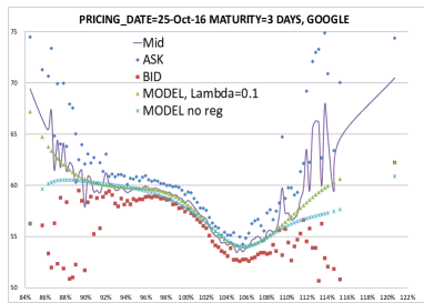
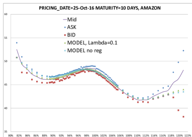
Figure 1. Computational time = 0.1 s. Left: GOOGLE. Right: AMAZON. The plots denoted “Model no reg” mean that we have chosen $\Lambda=\infty$.

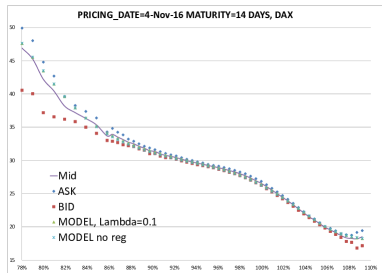
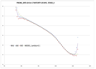
Figure 2. Computational time = 0.1 s. Left: DAX. Right: EURO STOXX 50.

Below, we list some numerical examples involving numerous equity stocks/indices with various liquidity/maturities: Société Générale, Danone, Apple, SP500.

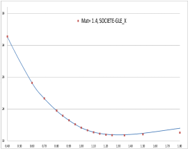
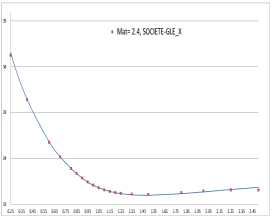
Figure 3. SOCIETE-GENERALE.

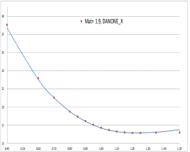
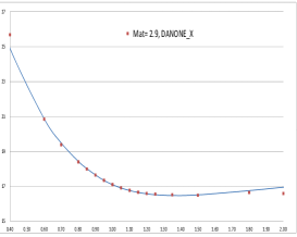
Figure 4. DANONE.

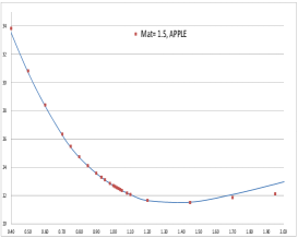
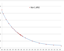
Figure 5. APPLE.

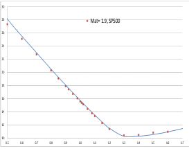
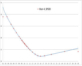
Figure 6. SP500.

5. Proofs of the results.

Lemma 5.1.

Let $(u^{*},h^{*},V^{*})$ be a minimiser of ${\cal G}$, then if we define

$$\mathbb{P}^{*}(ds_{1},ds_{2}) := {m_{0}}(ds_{1},ds_{2})e^{-\sum_{K\in{\cal K}}V_{K}^{*}(s_{2}-K)_{+}-u^{*}(s_{1})-h^{*}(s_{1})(s_{2}-s_{1})},$$

We have $\mathbb{P}^{*}\in\widetilde{\cal M}$.

Proof. The constraints are given by the Lagrange equations. For $s_{1}\in{\rm supp}({\mathbb{P}}^{1})$, the fact that ${\mathbb{P}}^{*}(S_{1}=s_{1})={\mathbb{P}}^{1}[s_{1}]$ is given by the equation $\partial_{u(s_{1})}{\cal G}(u^{*},h^{*},V^{*})$. The fact that $\mathbb{E}^{{\mathbb{P}}^{*}}[S_{2}|S_{1}=s_{1}]=s_{1}$ is given by the equation $\partial_{h(s_{1})}{\cal G}(u^{*},h^{*},V^{*})=0$. Finally, ${\cal C}^{K,{\rm bid}}\leq\mathbb{E}^{{\mathbb{P}}^{*}}[(S_{2}-K)_{+}]\leq{\cal C}^{K,{\rm ask}}$ is given by the equation $\partial_{V_{K}}{\cal G}(u^{*},h^{*},V^{*})=0$. $\Box$

Lemma 5.2.

The map ${\cal G}$ reaches a minimum ${\cal G}^{*}$ at some $x^{*}\in{\mathrm{L}}^{1}(\mathbb{P}^{1})^{2}\times\mathbb{R}^{|{\cal K}|}$ if and only if $\left(m_{0},{\mathbb{P}}^{1},\left({\cal C}^{K,{\rm bid/ask}}\right)_{K\in{\cal K}}\right)$ is non-degenerate.

Proof. Recall that as $u,h\in{\mathrm{L}}^{1}(\mathbb{P}^{1})$ can be identified with vectors in $\mathbb{R}^{|{\rm supp}({\mathbb{P}}^{1})|}$ as ${\mathbb{P}}^{1}$ has finite support.

Step 1: We assume that $\left(m_{0},{\mathbb{P}}^{1},\left({\cal C}^{K,{\rm bid/ask}}\right)_{K\in{\cal K}}\right)$ is non-degenerate. Let ${\cal C}\in\mathbb{R}^{|{\cal K}|}$ be a valid call prices vector. Let us prove that ${\cal G}$ reaches a minimum at some $x^{*}\in\mathbb{R}^{2|{\rm supp}({\mathbb{P}}^{1})|+|{\cal K}|}$. First we prove that $\lim_{|x|\to\infty}{\cal G}(x)=\infty$. Let $(x_{n})_{n\geq 0}\subset\mathbb{R}^{2|{\rm supp}({\mathbb{P}}^{1})|+|{\cal K}|}$ such that $|x_{n}|\longrightarrow\infty$. We assume for contradiction that up to replacing $x_{n}$ by a subsequence, ${\cal G}(x_{n})$ is bounded from above by $A>0$. Then up to taking a subsequence of $(x_{n})$, we may assume that $\frac{x_{n}}{|x_{n}|}$ converges to some $x\in{\cal U}:=\big{\{}x^{\prime}\in\mathbb{R}^{2|{\rm supp}({\mathbb{P}}^{1})|+|{\cal K}|}\big{\}}$. Now let the random vector

$$\Delta := \big{(}(\delta_{S_{1}=s_{1}})_{s_{1}\in{\rm supp}({\mathbb{P}}^{1})},(\delta_{S_{1}=s_{1}}(S_{2}-S_{1}))_{s_{1}\in{\rm supp}({\mathbb{P}}^{1})},((S_{2}-K)_{+})_{K\in{\cal K}}\big{)},$$

so that for $\big{(}(x_{1,s_{1}})_{s_{1}\in{\rm supp}({\mathbb{P}}^{1})},(x_{2,s_{1}})_{s_{1}\in{\rm supp}({\mathbb{P}}^{1})},(x_{3,K})_{K\in{\cal K}}\big{)}:=x\in\mathbb{R}^{2|\mathcal{X}_{1}|+|{\cal K}|}$, we have

$$x\cdot\Delta = x_{1,S_{1}}+x_{2,S_{1}}(S_{2}-S_{1})+\sum_{K\in{\cal K}}x_{3,K}(S_{2}-K)_{+}.$$

and

$${\cal G}(x) = \sum_{s_{1}\in{\rm supp}({\mathbb{P}}^{1})}x_{1,s_{1}}{\mathbb{P}}^{1}[s_{1}]+\sum_{K\in{\cal K}}f_{2}^{K,\mathrm{bid}/\mathrm{ask}}(x_{3,K},\omega_{K})+\sum_{K\in{\cal K}}x_{3,K}{\cal C}^{K,\mathrm{mid}}+\int e^{-x\cdot\Delta}d{m_{0}}.$$

Notice that as ${\cal C}^{K_{i},{\rm bid}}\leq{\cal C}_{i}\leq{\cal C}^{K_{i},{\rm ask}}$ for $1\leq i\leq k$, we have that $({\cal C}_{i})_{1\leq i\leq k}$ is the subgradient of $V\longmapsto\sum_{K\in{\cal K}}f_{2}^{K,\mathrm{bid}/\mathrm{ask}}(V_{K},\omega_{K})+\sum_{K\in{\cal K}}V_{K}{\cal C}^{K,\mathrm{mid}}$ at some point $V^{0}\in\mathbb{R}^{|{\cal K}|}$. Then if we denote $b:=\sum_{K\in{\cal K}}f_{2}^{K,\mathrm{bid}/\mathrm{ask}}(V^{0}_{K},\omega_{K})+\sum_{K\in{\cal K}}V^{0}_{K}{\cal C}^{K,\mathrm{mid}}$ and $a:=\big{(}({\mathbb{P}}^{1}[s_{1}])_{s_{1}\in{\rm supp}({\mathbb{P}}^{1})},0,({\cal C}_{i})_{1\leq i\leq k}\big{)}$, we have

(5.6) $${\cal G}(x)\geq a\cdot x+b+\int e^{-x\cdot\Delta}d{m_{0}}.$$

Case 1: We may find $(s_{1},s_{2})\in{\rm supp}({\mathbb{P}}^{1})\times\mathbb{R}_{+}$ such that $x\cdot\Delta(s_{1},s_{2})<0$. As $x\cdot\Delta(s_{1},\cdot)$ is affine by parts, we may find $\varepsilon>0$ and an open interval $s_{2}\in I\subset\mathbb{R}$ such that $x\cdot\Delta(s_{1},\cdot)\leq-\varepsilon$ on $I$. Then for $x^{\prime}$ close enough to $x$, we have $x^{\prime}\cdot\Delta(s_{1},\cdot)\leq-\frac{1}{2}\varepsilon$ on $I$. Then by (5.6), for $n$ large enough we have

$${\cal G}(x_{n}) \geq a\cdot x_{n}+b+\int e^{-x_{n}\cdot\Delta}d{m_{0}}$$

$$\geq a\cdot x_{n}+b+{m_{0}}[\{y_{1}\}\times I]e^{|x_{n}|\frac{1}{2}\varepsilon}.$$

Therefore, by the fact that ${m_{0}}[\{s_{1}\}\times I]>0$, we have that ${\cal G}(x_{n})$ diverges to $\infty$ as $|x_{n}|\longrightarrow\infty$, a contradiction.

Case 2: $x\cdot\Delta\geq 0$ on ${\rm supp}({\mathbb{P}}^{1})\times\mathbb{R}_{+}$. Then ${\cal G}(x_{n})\geq a\cdot x_{n}+b=|x_{n}|a\cdot\frac{x_{n}}{|x_{n}|}+b$. As we assumed that ${\cal G}(x_{n})$ is bounded and $\frac{x_{n}}{|x_{n}|}$ converges to $x$, we have

(5.7) $$a\cdot x\leq 0.$$

We denote $(u,h,V):=x$, identifying $u$ and $h$ as functions ${\rm supp}({\mathbb{P}}^{1})\longrightarrow\mathbb{R}$, and we have

$$x\cdot\Delta=u(S_{1})+h(S_{1})(S_{2}-S_{1})+\sum_{K\in{\cal K}}V_{K}(S_{2}-K)_{+}.$$

Let $\psi:=s\mapsto\sum_{K\in{\cal K}}V_{K}(s-K)_{+}$. We have $\psi(S_{2})\geq-u(S_{1})-h(S_{1})(S_{2}-S_{1})$. Then if we denote $f$, the convex hull of $\psi$ on $\mathbb{R}_{+}$, we have $\psi\geq f$ and for all $s_{1}\in\mathcal{X}_{1}$, we have $f(S_{2})\geq-u(s_{1})-h(s_{1})\cdot(S_{2}-s_{1})$. Therefore, $f\geq-u$ from last functional inequality computed in $S_{2}=s_{1}$. By the fact that $f$ is the convex hull of $\psi$, which is piecewise affine, $f$ is also piecewise affine on the same intervals. Therefore, by using the notation ${\cal K}=(K_{i})_{1\leq i\leq k}$ from Definition 3.1, we may find $\lambda_{i}\geq 0$ for all $1\leq i\leq k$ such that $f=s\mapsto f(0)+\nabla f(0)s+\sum_{i=1}\lambda_{i}(s-K_{i})_{+}$. Recall that by Definition 3.1 we have that ${\cal C}_{0}=\mathbb{E}^{{\mathbb{P}}_{1}}[S_{1}]$, and ${\cal C}_{k+1}=1$, thus we have

$$a\cdot x = \mathbb{E}^{{\mathbb{P}}^{1}}[u+f]+\sum_{i=0}^{k}\mu_{i}{\cal C}_{i}+\sum_{i=1}^{k+1}\lambda_{i}\big{(}{\cal C}_{i}-\mathbb{E}^{{\mathbb{P}}^{1}}[(S_{2}-K_{i})_{+}]\big{)},$$

where $\mu_{0}:=-\nabla f(0)$, $\mu_{k+1}:=-f(0)$, and $\mu_{i}:=V_{K_{i}}-\lambda_{i}$ for $1\leq i\leq k$ are the unique coefficients such that

(5.8) $$(\psi-f)(S_{2})=\sum_{i=0}^{k}\mu_{i}(S_{2}-K_{i})_{+}.$$

Notice that $(\psi-f)\geq 0$, therefore for all $0\leq i\leq k+1$, $\gamma_{i}:=(\psi-f)(K_{i+1})=(M_{\rm call}^{t}\mu)_{i}\geq 0$ by evaluating (5.8) in each $K_{i}$, where recall the definition of $M_{\rm call}$ and the conventions on $i=k+1$ from Definition 3.1. Then $\mu=(M_{\rm call}^{t})^{-1}\gamma$, and $\mu\cdot{\cal C}=(M_{\rm call}^{-1}{\cal C})\cdot\gamma$. Finally,

$$a\cdot x=\mathbb{E}^{{\mathbb{P}}^{1}}[u+f]+(M_{\rm call}^{-1}{\cal C})\cdot\gamma+\sum_{i=1}^{k}\lambda_{i}\big{(}{\cal C}_{i}-\mathbb{E}^{{\mathbb{P}}^{1}}[(S_{2}-K_{i})_{+}]\big{)}.$$

By (5.7), $a\cdot x$ is non-positive, therefore, the non-degeneracy of ${\cal C}$ gives that $\lambda_{1}=...=\lambda_{k}=0$, $\gamma=0$, and $u+f=0$. Therefore $\mu=0$, $f=0$, $u=-f=0$, $V=0$. Therefore, $x\cdot\Delta=h(S_{1})(S_{2}-S_{1})$. By the fact that $x\cdot\Delta\geq 0$, $m_{0}-$a.e., (vi) from Definition 3.1 implies that we have that $h=0$. Finally $x\cdot\Delta=0$ on $\mathcal{X}_{1}\times\mathbb{R}_{+}$, and finally $x=0$, which is a contradiction as $x\in{\cal U}$.

We proved that $\lim_{|x|\to\infty}{\cal G}(x)=\infty$. As ${\cal G}$ is convex, it reaches a minimum at some $x^{*}\in\mathbb{R}^{2|{\rm supp}({\mathbb{P}}^{1})|+|{\cal K}|}$.

Step 2: Now we assume that ${\cal G}$ reaches a minimum. Let us denote $x^{*}$ this minimum and let $\mathbb{P}^{*}(ds_{1},ds_{2})={m_{0}}(ds_{1},ds_{2})e^{-\sum_{K\in{\cal K}}V_{K}^{*}(s_{2}-K)_{+}-u^{*}(s_{1})-h^{*}(s_{1})(s_{2}-s_{1})}$. By Lemma 5.1, we have that ${\mathbb{P}}^{*}\in\widetilde{\cal M}$. Notice also that the measure ${\mathbb{P}}^{*}$ is equivalent to the measure $m_{0}$. Therefore, for all $i$ the map $\theta_{i}:=(S_{2}-K_{i})_{+}-(S_{1}-K_{i})_{+}-\mathbf{1}_{S_{1}\geq K_{i}}(S_{2}-S_{1})$ is non-negative and non-(zero ${\mathbb{P}}^{*}-$a.e.). Therefore $\mathbb{E}^{{\mathbb{P}}^{*}}[\theta_{i}]>0$. Finally we observe that if we denote ${\cal C}_{i}:=\mathbb{E}^{{\mathbb{P}}^{*}}[(S_{2}-K)_{+}]$, then we have $\mathbb{E}^{{\mathbb{P}}^{*}}[\theta_{i}]={\cal C}_{i}-\mathbb{E}^{{\mathbb{P}}^{1}}[(S_{1}-K)_{+}]$ from the martingale property of ${\mathbb{P}}^{*}$, and ${\cal C}^{K_{i},{\rm bid}}\leq{\cal C}_{i}\leq{\cal C}^{K_{i},{\rm ask}}$ as ${\mathbb{P}}^{*}\in\widetilde{\cal M}$. Now for $1\leq i\leq k$, let $f_{i}$ the piecewise affine map such that $f$ is zero on $[0,K_{i-1}]$, with $f(K_{i})=1$, affine on $[K_{i-1},K_{i}]$, $[K_{i},K_{i+1}]$, and $[K_{i+1},\infty)$, if $i\neq k$, and $f_{k}$ is constant equal to $1$ on $[K_{k},\infty]$. We observe that for all $i$, $f_{i}$ is non-negative and non-zero ${\mathbb{P}}^{*}-$a.e. Furthermore, $0<\mathbb{E}^{{\mathbb{P}}^{*}}[f_{i}]=(M_{\rm call}^{-1}{\cal C})_{i}$. We proved that $\left(m_{0},{\mathbb{P}}^{1},\left({\cal C}^{K,{\rm bid/ask}}\right)_{K\in{\cal K}}\right)$ is non-degenerate as the other properties are obvious. $\Box$

Proof of Theorem 3.3 By introducing dual variables $u^{\rm bid},u^{\rm ask}\in({\mathbb{R}}_{+})^{{\cal K}}$ for the inequalities for the call prices at bid and at ask, $\inf{\cal G}$ may be written as

$$\inf{\cal G} = -\inf_{u^{\rm bid},u^{\rm ask}\in({\mathbb{R}}_{+})^{{\cal K}},v_{K}\in{\mathbb{R}},u,h\in{\mathbb{R}}^{{\rm supp}({\mathbb{P}}^{1})}}\mathbb{E}^{{\mathbb{P}}^{1}}[u(S_{1})]+\sum_{K\in{\cal K}_{1}}u_{K}^{\rm ask}{\cal C}^{\mathrm{ask}}_{K}-u_{K}^{\rm bid}{\cal C}^{\mathrm{bid}}_{K}+v_{K}{\cal C}^{\mathrm{mid}}_{K}$$

$$+\frac{1}{2}v_{K}^{2}\omega_{K}+{\mathbb{E}}^{{m_{0}}}\left[e^{-\sum_{K\in{\cal K}}(u_{K}^{\rm ask}-u_{K}^{\rm bid}+v_{K})(S_{1}-K)_{+}-u(S_{1})-h(S_{1})(S_{2}-S_{1})}\right].$$

By setting $v:=V-u^{\rm ask}+u^{\rm bid}$, the function, to be minimized, is equivalent to

$$\mathbb{E}^{{\mathbb{P}}^{1}}[u(S_{1})]+\sum_{K\in{\cal K}_{1}}u^{\rm ask}_{K}({\cal C}_{1}^{K,\mathrm{ask}}-{\cal C}_{1}^{K,\mathrm{mid}})-u^{\rm bid}_{K}({\cal C}_{1}^{K,\mathrm{bid}}-{\cal C}_{1}^{K,\mathrm{mid}})+V_{K}{\cal C}_{1}^{K,\mathrm{mid}}$$

$$+ \frac{1}{2}(V-u^{\rm ask}+u^{\rm bid})^{2}\cdot\omega+{\mathbb{E}}^{{m_{0}}}\left[e^{-\sum_{K\in{\cal K}}V_{K}(S_{1}-K)_{+}-u(S_{1})-h(S_{1})(S_{2}-S_{1})}\right].$$

We observe that the minimization over $u^{\rm ask}$ and $u^{\rm bid}$ can be exactly performed and we obtain finally an unconstrained optimization over $V$.

By Lemma 5.2, the non degeneracy of $\left(m_{0},{\mathbb{P}}^{1},\left({\cal C}^{K,{\rm bid/ask}}\right)_{K\in{\cal K}}\right)$ implies that ${\cal G}$ reaches a minimum. Let $\mathbb{P}^{*}\in\widetilde{\cal M}$ from Lemma 5.1, ${\mathbb{P}}^{*}$ is the optimiser of (3.2) from Proposition 1 in [2]. $\Box$

Proof of Theorem 3.4 The first equivalence is given by Lemma 5.2.

Step 1: The convergence result stems from an indirect application of Theorem 5.2 in [4]. By a direct application of this theorem we get that

(5.9) $${\cal G}(x_{k})-{\cal G}(x^{*})\leq\left(1-\frac{\sigma}{\min(L_{1},L_{2})}\right)^{n-1}\big{(}{\cal G}(x_{0})-{\cal G}(x^{*})\big{)},$$

with $L_{1}$ (resp. $L_{2}$) is the Lipschitz constant of the $V-$gradient (resp. $(u,h)-$gradient) of ${\cal G}$, and $\sigma$ is the strong convexity parameter of ${\cal G}$. Furthermore, the strong convexity gives that

(5.10) $$|x_{k}-x^{*}|\leq\sqrt{\frac{2}{\sigma}}\big{(}{\cal G}(x_{k})-{\cal G}(x^{*})\big{)}^{\frac{1}{2}}.$$

Finally, by definition of $L_{1}$ and $L_{2}$, we have

(5.11) $$|\nabla{\cal G}(x_{k})|\leq(L_{1}+L_{2})|x_{k}-x^{*}|.$$

These inequalities would prove the theorem with

$$\lambda=1-\frac{\sigma}{\min(L_{1},L_{2})} M=(L_{1}+L_{2}+1)\sqrt{\frac{2}{\sigma}}.$$ and

However the gradient $\nabla{\cal G}$ is locally but not globally Lipschitz, nor ${\cal G}$ strongly convex. Therefore we need to refine the theorem by looking carefully at where these constants are used in its proof.

Step 2: The constant $L_{1}$ is used for Lemma 5.1 in [4]. We need for all $k\geq 0$ to have ${\cal G}(x_{k})-{\cal G}(x_{k+1/2})\geq\frac{1}{2L_{1}}|\nabla{\cal G}(x_{k})|^{2}$. We want to find $C,L>0$ such that ${\cal G}(x_{k})-{\cal G}\big{(}x_{k}-C\nabla{\cal G}(x_{k})\big{)}\geq\frac{1}{2L}|\nabla{\cal G}(x_{k})|$, then $L$ may be use to replace $L_{1}$ in the final step of the proof of Lemma 5.1 in [4]. By the fact that $\lim_{|x|\to\infty}{\cal G}(x)=\infty$, the set ${\mathfrak{C}}(x_{0}):=\{x\in\mathbb{R}^{2|{\rm supp}({\mathbb{P}}^{1})|+|{\cal K}|}:{\cal G}(x)\leq{\cal G}(x_{0})\}$ is compact. Then $\nabla{\cal G}$ is bounded on ${\mathfrak{C}}(x_{0})$. Therefore we may find $M_{1}>0$ such that for all $k$, we have $|\nabla{\cal G}(x_{k})\cdot\Delta|\leq M_{1}(1+|S_{2}|)$ where we denote $\Delta$ the random vector

$$\Delta := \big{(}(\delta_{S_{1}=s_{1}})_{s_{1}\in{\rm supp}({\mathbb{P}}^{1})},(\delta_{S_{1}=s_{1}}(S_{2}-S_{1}))_{s_{1}\in{\rm supp}({\mathbb{P}}^{1})},((S_{2}-K)_{+})_{K\in{\cal K}}\big{)}.$$

Furthermore, let $F(C):=\sup_{(u,x)\in{\cal U}\times{\mathfrak{C}}(x_{0})}\int_{0}^{1}\int(u\cdot\Delta)e^{-x\cdot\Delta}e^{tCM_{1}(1+|S_{2}|)}dm_{0}dt$. We have

$${\cal G}(x_{k})-{\cal G}\big{(}x_{k}-C\nabla{\cal G}(x_{k}),h_{k}\big{)} = \nabla{\cal G}(x_{k})\cdot\big{(}-C\nabla{\cal G}(x_{k})\big{)}$$

$$-C^{2}\int_{0}^{1}(1-t)D^{2}{\cal G}\big{(}x_{k}-tC\nabla{\cal G}(x_{k})\big{)}\big{(}\nabla{\cal G}(x_{k})\big{)}^{2}dt$$

$$= C|\nabla{\cal G}(x_{k})|^{2}$$

$$-C^{2}\int_{0}^{1}(1-t)\int(\nabla{\cal G}(x_{k})\cdot\Delta)^{2}e^{-x_{k}\cdot\Delta}e^{tC\nabla{\cal G}(x_{k})\cdot\Delta}dm_{0}dt$$

$$\geq C|\nabla{\cal G}(x_{k})|^{2}-C^{2}|\nabla{\cal G}(x_{k})|^{2}F(C)$$

$$= \big{(}C-C^{2}F(C)\big{)}|\nabla{\cal G}(x_{k})|^{2}.$$

As $F$ is non-decreasing finite, then when $C\longrightarrow 0$ we have $\frac{C-C^{2}F(C)}{C}\longrightarrow 1$. Then for $C$ small enough, let $L:=\frac{1}{2\big{(}C-C^{2}F(C)\big{)}}>0$. We get

$${\cal G}(x_{k})-{\cal G}\big{(}x_{k}-C\nabla{\cal G}(x_{k})\big{)}\geq\frac{1}{2L}|\nabla{\cal G}(x_{k})|^{2}.$$

Step 3: The constant $\sigma$ is used to get the result from (3.21) in [4]. Then we just need the inequality

(5.12) $${\cal G}(y)\geq{\cal G}(x)+\nabla{\cal G}(x)\cdot(y-x)+\frac{\sigma}{2}|y-x|^{2},$$

to hold for some $y=x^{*}$ and $x=x_{k}$ for all $k\geq 0$. Now we give a lower bound for $\sigma$. The map $(u,x)\longmapsto D^{2}{\cal G}(x)u^{2}=\int(u\cdot\Delta)^{2}e^{-x\cdot\Delta}dm_{0}>0$ is continuous on ${\cal U}\times{\mathfrak{C}}(x_{0})$ compact, therefore it has a lower bound $\sigma>0$. This constant also works for (5.10). Similar, $\sup_{(u,x)\in{\cal U}\times{\mathfrak{C}}(x_{0})}D^{2}{\cal G}(x)u^{2}$ may replace $L_{1}+L_{2}$ from (5.11).

Step 4: Finally, as we focus on the $L_{1}$ optimization phase, we may replace $n-1$ by $n$ in the convergence formula (5.9), see the proof of Theorem 5.2 in [4].

Now the existence of $M>0$ stems from the facts that ${\cal G}(x_{k})-{\cal G}(x^{*})\geq\frac{1}{2}\sigma|x_{k}-x^{*}|^{2}$, and $|\nabla{\cal G}(x_{k})|\leq L|x_{k}-x^{*}|$.

Step 5: Now we just use the fact that

$$\nabla{\cal G} = \sum_{s_{1}\in{\rm supp}({\mathbb{P}}^{1})}\left({\mathbb{P}}^{1}[\{s_{1}\}]-{\mathbb{P}}_{n}\circ(S_{1})^{-1}[\{s_{1}\}]\right)e_{s_{1}}$$

$$+\sum_{s_{1}\in{\rm supp}({\mathbb{P}}^{1})}\left(\mathbb{E}^{{\mathbb{P}}_{n}}[S_{2}-s_{1},S_{1}=s_{1}]\right)e_{|{\rm supp}({\mathbb{P}}^{1})|+s_{1}}$$

$$+\sum_{i=1}^{k}\left(C_{K}-\mathbb{E}^{{\mathbb{P}}_{n}}[(S_{2}-K_{i})_{+}]\right)e_{2|{\rm supp}({\mathbb{P}}^{1})|+i},$$

where $C_{K}\in[{\cal C}^{K,{\rm bid}},{\cal C}^{K,{\rm ask}}]$, and $(e_{i})_{1\leq i\leq 2|{\rm supp}({\mathbb{P}}^{1})|+|{\cal K}|}$ is the canonical basis. Therefore, this gradient is a crucial estimate of the mismatch of ${\mathbb{P}}$ in terms of first marginal, martingale property, and correctness of the call prices it gives. However, as we consider $x_{n}$ after the Bregman projection from the Sinkorn’s algorithm on $u_{n}$ and $h_{n}$, ${\mathbb{P}}_{n}$ is martingale as minimal in $h_{n}$, and has marginal ${\mathbb{P}}^{1}$ on $S_{1}$ as minimal in $u_{n}$. Then $\nabla{\cal G}=\sum_{i=1}^{k}\left(C_{K}-\mathbb{E}^{{\mathbb{P}}_{n}}[(S_{2}-K_{i})_{+}]\right)e_{2|{\rm supp}({\mathbb{P}}^{1})|+i}$. We obtain the inequality by taking the infinite norm on this vector, that is equivalent to any other as we are in finite dimensions. Therefore up to raising $M>0$, the result is proved. $\Box$

Proof of Theorem 3.9 We build the probabilities ${\mathbb{P}}_{i}$ by induction. We first set ${\mathbb{P}}_{0}:=\delta_{S_{0}}$.

Now let $1\leq i\leq n-1$ we assume that ${\mathbb{P}}_{0},...,{\mathbb{P}}_{i-1}$ are created, that the results of the Theorem is proved for them, and that they satisfy that $\left(m^{j-1,j},{\mathbb{P}}_{j-1},\left({\cal C}^{K,{\rm bid/ask}}\right)_{K\in{\cal K}_{j}}\right)$ is non-degenerate for $j\leq i-1$.

We first prove the non-degeneracy of $\left(m^{i-1,i},{\mathbb{P}}_{i-1},\left({\cal C}^{K,{\rm bid/ask}}\right)_{K\in{\cal K}_{i}}\right)$. For this we need to prove (i) to (vi) from Definition 3.1. Thanks to the non-degeneracy of $\left(m_{n},\left({\cal C}^{K,{\rm bid/ask}}_{i}\right)_{1\leq i\leq n,K\in{\cal K}_{i}}\right)$, we set ${\cal C}:={\cal C}^{i}$ from Definition 3.8.

(i) holds by (i) of Definition 3.8 for $1\leq l\leq k$. For $l=0$, if $i=1$, the result is trivial as $\mathbb{E}^{{\mathbb{P}}_{0}}[S_{0}]=S_{0}$. For $i\geq 1$, we have that $\mathbb{E}^{{\mathbb{P}}_{i-2}}[S_{t_{i-1}}]=S_{0}$ by induction assumption, then as ${\mathbb{P}}_{i-1}={\mathbb{P}}_{i-2}{\mathbb{P}}^{i-2,i-1}(ds_{i-1}|s_{i-2})$ with ${\mathbb{P}}^{i-2,i-1}$ martingale by induction assumption together with Definition 3.8, we have

$${\cal C}^{0,{\rm bid}}_{i}={\cal C}^{0,{\rm ask}}_{i}=\mathbb{E}^{{\mathbb{P}}_{i-1}}[S_{t_{i-1}}]=S_{0}=\mathbb{E}^{{\mathbb{P}}_{i-2}}[S_{t_{i-1}}]=S_{0}.$$

The case $l=k+1$ is also trivial from Definition 3.8.

(ii) holds by (ii) of Definition 3.8.

(iii) Let $1\leq l\leq k$, we have that $(S_{t_{i-1}}-K_{l})_{+}\leq(S_{t_{i-1}}-K^{i-1}_{l^{\prime}})_{+}+(K^{i-1}_{l^{\prime}}-K_{l})_{+}$ where we take $K^{i-1}_{l^{\prime}}$ from (iii) in Definition 3.8. Then we have thanks to (iii) in Definition 3.8:

$$\mathbb{E}^{{\mathbb{P}}_{i-1}}[(S_{t_{i-1}}-K_{l})_{+}] \leq \mathbb{E}^{{\mathbb{P}}_{i-1}}[(S_{t_{i-1}}-K^{i-1}_{l^{\prime}})_{+}]+(K^{i-1}_{l^{\prime}}-K_{l})_{+}$$

$$\leq {\cal C}^{K^{i-1}_{l^{\prime}},\rm ask}_{i-1}+(K^{i-1}_{l^{\prime}}-K_{l})_{+}$$

$$< {\cal C}^{K_{l},\rm bid}$$

$$\leq {\cal C}_{l}.$$

(iii) is proved.

(iv) As by induction assumption, $\frac{d{\mathbb{P}}^{i-2,i-1}}{dm^{i-2,i-1}}>0$, $dm^{i-2,i-1}-$a.s. Therefore,

$${\rm supp{\mathbb{P}}^{i-1}} = {\rm supp{\mathbb{P}}^{i-2,i-1}\circ S_{t_{i-1}}^{-1}}$$

$$= {\rm suppm^{i-2,i-1}\circ S_{t_{i-1}}^{-1}}$$

$$= {\rm suppm^{i-1,i-2}\circ S_{t_{i-1}}^{-1}}.$$

by (iv) of Definition 3.8. (iv) is proved.

(v) holds by (v) of Definition 3.8.

(vi) holds by (vi) of Definition 3.8.

The non degeneracy of $\left(m^{i-1,i},{\mathbb{P}}_{i-1},\left({\cal C}^{K,{\rm bid/ask}}\right)_{K\in{\cal K}_{i}}\right)$ allows to apply Theorem 3.3, which gives the rest of the result of the Theorem for $i-1$. The Theorem is then proved by induction. $\Box$

References

• [1] Jesper Andreasen and Brian Huge. Expanded forward volatility. Risk, 26(1):101, 2013.
• [2] M Avellaneda. Minimum entropy calibration of asset pricing models, internat. J. Theoret. Appl. Finance, 1:447472, 1998.
• [3] Marco Avellaneda, Robert Buff, Craig Friedman, Nicolas Grandechamp, Lukasz Kruk, and Joshua Newman. Weighted monte carlo: a new technique for calibrating asset-pricing models. International Journal of Theoretical and Applied Finance, 4(01):91–119, 2001.
• [4] Amir Beck and Luba Tetruashvili. On the convergence of block coordinate descent type methods. SIAM journal on Optimization, 23(4):2037–2060, 2013.
• [5] Jean-David Benamou, Guillaume Carlier, Marco Cuturi, Luca Nenna, and Gabriel Peyré. Iterative bregman projections for regularized transportation problems. SIAM Journal on Scientific Computing, 37(2):A1111–A1138, 2015.
• [6] Peter Carr and Dilip B Madan. A note on sufficient conditions for no arbitrage. Finance Research Letters, 2(3):125–130, 2005.
• [7] Laurent Cousot. Conditions on option prices for absence of arbitrage and exact calibration. Journal of Banking & Finance, 31(11):3377–3397, 2007.
• [8] Marco Cuturi. Sinkhorn distances: Lightspeed computation of optimal transport. In Advances in neural information processing systems, pages 2292–2300, 2013.
• [9] Hadrien De March. Entropic resolution for multi-dimensional optimal transport. arXiv preprint arXiv:1812.11104, 2018.
• [10] Bruno Dupire. Pricing and hedging with smiles. Mathematics of derivative securities, 1(1):103–111, 1997.
• [11] Peter K Friz, Jim Gatheral, Archil Gulisashvili, Antoine Jacquier, and Josef Teichmann. Large deviations and asymptotic methods in finance, volume 110. Springer, 2015.
• [12] Jim Gatheral and Antoine Jacquier. Convergence of heston to svi. Quantitative Finance, 11(8):1129–1132, 2011.
• [13] Jim Gatheral and Antoine Jacquier. Arbitrage-free svi volatility surfaces. Quantitative Finance, 14(1):59–71, 2014.
• [14] Gaoyue Guo and Jan Obloj. Computational methods for martingale optimal transport problems. arXiv preprint arXiv:1710.07911, 2017.
• [15] Pierre Henry-Labordère. Analysis, geometry, and modeling in finance: Advanced methods in option pricing. Chapman and Hall/CRC, 2008.
• [16] Pierre Henry-Labordere. Calibration of local stochastic volatility models to market smiles: A monte-carlo approach. 2009.
• [17] Pierre Henry-Labordere and Nizar Touzi. An explicit martingale version of brenier’s theorem. 2013.
• [18] Sigrid Källblad, Xiaolu Tan, Nizar Touzi, et al. Optimal skorokhod embedding given full marginals and azéma–yor peacocks. The Annals of Applied Probability, 27(2):686–719, 2017.
• [19] Alex Lipton and Artur Sepp. Filling the gaps. 2011.
• [20] Alexander Lipton. Masterclass with deutsche bank. the vol smile problem. RISK-LONDON-RISK MAGAZINE LIMITED-, 15(2):61–66, 2002.
• [21] Quentin Mérigot. A multiscale approach to optimal transport. In Computer Graphics Forum, volume 30, pages 1583–1592. Wiley Online Library, 2011.
• [22] Gabriel Peyré, Marco Cuturi, et al. Computational optimal transport. Technical report, 2017.
• [23] Bernhard Schmitzer. Stabilized sparse scaling algorithms for entropy regularized transport problems. arXiv preprint arXiv:1610.06519, 2016.
• [24] Richard Sinkhorn and Paul Knopp. Concerning nonnegative matrices and doubly stochastic matrices. Pacific Journal of Mathematics, 21(2):343–348, 1967.
• [25] Volker Strassen. The existence of probability measures with given marginals. The Annals of Mathematical Statistics, pages 423–439, 1965.