Solar wind charge exchange in cometary atmospheres

Abstract

Context. Solar wind charge-changing reactions are of paramount importance to the physico-chemistry of the atmosphere of a comet. The ESA/Rosetta mission to comet 67P/Churyumov-Gerasimenko (67P) provides a unique opportunity to study charge-changing processes in situ.

Aims. To understand the role of these reactions in the evolution of the solar wind plasma and interpret the complex in situ measurements made by Rosetta, numerical or analytical models are necessary.

Methods. We used an extended analytical formalism describing solar wind charge-changing processes at comets along solar wind streamlines. The model is driven by solar wind ion measurements from the Rosetta Plasma Consortium-Ion Composition Analyser (RPC-ICA) and neutral density observations from the Rosetta Spectrometer for Ion and Neutral Analysis-Comet Pressure Sensor (ROSINA-COPS), as well as by charge-changing cross sections of hydrogen and helium particles in a water gas.

Results. A mission-wide overview of charge-changing efficiencies at comet 67P is presented. Electron capture cross sections dominate and favor the production of He and H energetic neutral atoms (ENAs), with fluxes expected to rival those of H⁺ and He²⁺ ions.

Conclusions. Neutral outgassing rates are retrieved from local RPC-ICA flux measurements and match ROSINA estimates very well throughout the mission. From the model, we find that solar wind charge exchange is unable to fully explain the magnitude of the sharp drop in solar wind ion fluxes observed by Rosetta for heliocentric distances below $2.5$ AU. This is likely because the model does not take the relative ion dynamics into account and to a lesser extent because it ignores the formation of bow-shock-like structures upstream of the nucleus. This work also shows that the ionization by solar extreme-ultraviolet radiation and energetic electrons dominates the source of cometary ions, although solar wind contributions may be significant during isolated events.

1 Introduction

Between August 2014 and its controlled end-of-mission crash on 30 September 2016, the European Space Agency mission Rosetta accompanied comet 67P/Churyumov-Gerasimenko (67P) on its journey toward the inner solar system, through perihelion at $1.24$ astronomical units (AU), and back out again (Jones et al., 2017; Taylor et al., 2017). During this period, Rosetta monitored in situ the neutral and plasma environment of the comet and its interaction with the solar wind, using dedicated instruments (Glassmeier, 2017).

A relevant process in the collisional interaction between a neutral environment and the solar wind is charge exchange (see Dennerl, 2010). In the following, ”charge exchange” and ”charge transfer” are used interchangeably to denote electron capture reactions only, whereas charge-changing collisions encompass both electron capture and stripping reactions. In cometary or planetary atmospheres, charge-exchange reactions, such as single or multiple electron captures, result in the creation of slow cometary ions, arising from collisions between fast solar wind ions and the slow-moving neutral gas. In the process, solar wind ions may become excited and emit radiation in the form of soft X-rays (see Cravens & Gombosi, 2004, and references therein). For a solar wind made of Xⁱ⁺ ions impacting a neutral gas species M, the electron capture of $q$ electrons is

$$\textnormal{X}^{i+}+\textnormal{M} \longrightarrow\textnormal{X}^{(i-q)+}+[\textnormal{M}]^{q+},$$ (1)

with ”[M]” referring to the possibility for compound M to undergo, in the process, dissociation, excitation, and ionization, or a combination of these processes. Such a reaction for the solar wind is referred to as ”solar wind charge exchange”, abbreviated SWCX, to distinguish it from other charge-exchange processes involving, for instance, fast cometary ions and the slow-moving neutral gas. In the latter case, in the inner coma of a comet, where the solar wind is expected to be significantly slowed down as is the case for high-activity comets (such as 1P/Halley), charge exchange between cometary ions and neutrals may also play a role in converting fast cometary ions, which have been accelerated by local electric fields, into slow ones, potentially ensuring that the cometary plasma moves with the neutrals.

Because the neutral atmosphere of a comet is in expansion and may extend to millions of kilometers in space (Combi et al., 2004), SWCX reactions may strongly affect the solar wind mass-loading upstream of the nucleus, and thus the formation and dynamics of bow shock and cometopause structures (Gombosi, 1987; Simon Wedlund et al., 2017), and around the diamagnetic cavity (Ip, 1990). Moreover, the projectile solar wind ion is usually much faster ($\sim 400$ km s^-1) than the neutral species it hits ($\sim 1$ km s^-1), with the result that the charge-exchanged species mostly keep their initial kinetic energy (Simon Wedlund et al., 2019b). Momentum transfer due to charge exchange between ion projectiles and neutral targets may also take place, and dominates at low impact energies the total momentum transfer cross sections (Banks & Kockarts, 1973; Ip, 1990).

As solar wind H⁺ and He²⁺ ions impinge upon an atmosphere, charge-changing reactions start fractionating the initial charge state distribution into a mixture of H⁺, H⁰ and H^- on the one hand, and of He²⁺, He⁺ and He⁰ species on the other (Simon Wedlund et al., 2019a). This effectively results in the production of fast energetic neutral atoms (ENAs), which are not bound to the plasma, but may interact further with the atmosphere downstream of the SWCX collision (see Fig. 1).

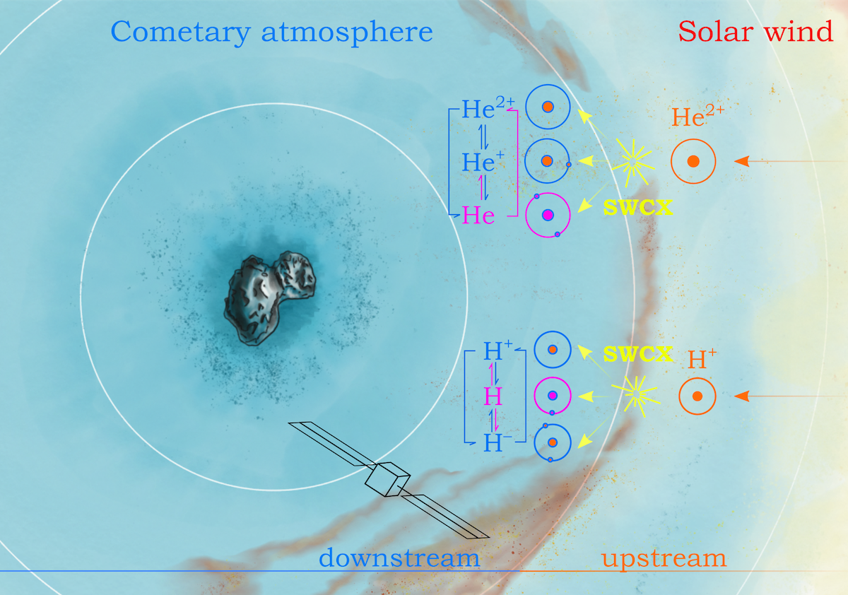
Figure 1: Sketch of solar wind charge-exchange interactions (SWCX) at comet 67P for a heliocentric distance of about $2$ AU. The upstream solar wind, composed of H⁺ and He²⁺ ions, experiences charge-changing collisions when impacting the comet’s neutral atmosphere, producing a mixture of charged states downstream of the collision. ENAs are depicted in pink. An increasingly deep blue color denotes a correspondingly denser atmosphere. SWCX plays a major role at and around the bow shock-like structure, depicted in shades of red, where the solar wind is heated and deflected.

A spacecraft such as Rosetta, which carried neutral, ion, and electron spectrometers deep in the atmosphere of comets or planets, can measure particle fluxes of individual charge states in situ (see Nilsson et al., 2007; Burch et al., 2007). One such instrument is, for example, the Rosetta Plasma Consortium Ion Composition Analyser (RPC-ICA) on board Rosetta. RPC-ICA is a top-hat mass spectrometer capable of simultaneously measuring the angular distribution of H⁺, He²⁺ , and He⁺ ion fluxes with good temporal resolution (Nilsson et al., 2015a, b; Behar et al., 2016b, a, 2017). A wide range of studies has been performed with it and includes: evidence of SWCX and a simple analytical model (Simon Wedlund et al., 2016), mass-loading of the solar wind (Behar et al., 2016a, b), characterization of the solar wind ion cavity (Behar et al., 2017), high temporal resolution of ion dynamics (Stenberg Wieser et al., 2017), cometary ion dynamics (Berčič et al., 2018), characterization of tail plasma (Behar et al., 2018a), and evidence for cometary bow shock detections (Gunell et al., 2018; Alho et al., 2019).

Another plasma instrument on board Rosetta capable of studying SWCX reactions is the RPC Ion and Electron Sensor (RPC-IES, Burch et al., 2007). Burch et al. (2015) detected H^- negative ions in the early phase of the mission for the first time. They were confirmed to be arising from two consecutive single-electron captures from the initial solar wind protons (Burch et al., 2015; Simon Wedlund et al., 2019a).

Complementing the pure plasma measurements, the neutral environment of the comet was probed using the mass spectrometers as part of the Rosetta Orbiter Spectrometer for Ion and Neutral Analysis (ROSINA, Balsiger et al., 2007). This instrument package measured the precise neutral composition of the cometary atmosphere, linked it to precise outgassing regions on the nucleus (Fougere et al., 2016; Läuter et al., 2019), and painted a picture of the complex interplay between the main species at the comet, namely H₂O, CO₂, CO, and O₂ (Bieler et al., 2015b, a). Its ion channel was also able to distinguish among heavy ions (e.g., H₂O⁺, H₃O⁺, CO${}_{2}^{+}$, and NH${}_{4}^{+}$) in the ionosphere (Fuselier et al., 2015, 2016; Beth et al., 2016).

The present work is the third of a series of studies on charge-changing reactions in cometary atmospheres, with application to the Rosetta datasets. It consists of three parts that we briefly describe below.

Simon Wedlund et al. (2019b) (hereafter Paper I) presented a review of currently available experimental charge-changing and ionization cross sections of hydrogen and helium species in a water gas, with recommended low-energy values for typical solar wind energies. As H₂O is the most abundant cometary neutral species during most of the Rosetta mission (Läuter et al., 2019), only this species was considered. Laboratory data needs were identified, which are required to bridge the gaps in the current experimental results. Polynomial fits for the systems $(\textnormal{H}^{+},\textnormal{H},\textnormal{and H}^{-})-\textnormal{H}_{2}\textnormal{O}$ and $(\textnormal{He}^{2+},\textnormal{He}^{+},\textnormal{and He})-\textnormal{H}_{2}\textnormal{O}$ were proposed. This cross section review is therefore not confined to comet-solar wind plasma interactions, but may hold interest for the astrophysics, biophysics, and atomic/molecular physics communities.

Simon Wedlund et al. (2019a) (hereafter Paper II) developed a general analytical solution of the three-species system of helium and hydrogen, with implications specific to comets. The forward model expressions were given, and two inversions, one for deriving the outgassing rate of the comet, one for estimating the upstream solar wind flux from in situ ion observations, were proposed. Using the recommended cross sections of Paper I, the dependence on heliocentric distance, cometocentric distance, and solar wind speed was explored. From geometrical considerations alone, predictions for the charge state distribution at comet 67P at the location of Rosetta were given.

In the present study, we apply the analytical forward and inverse models of Paper II to Rosetta’s ion and neutral observations. From local RPC-ICA ion flux measurements, we then retrieve the total neutral outgassing rate of comet 67P, which we compare to ROSINA neutral measurements. We also attempt to derive an estimate of the upstream solar wind flux from local ion measurements, with a comparison to solar wind flux estimates propagated from Mars and Earth. Finally, we present a mission overview of local ion productions due to SWCX and compare them to photoionization and electron impact ionization. In the closing paragraphs, we give mission-wide predictions on the ENA environment at the comet.

2 Model description

In order to describe how charge-transfer and stripping reactions impacted the solar wind plasma when it encountered the neutral environment of 67P during the Rosetta mission, we developed in Paper II a general 1D analytical solution of the three-charge component fluid system of hydrogen and helium solar wind particles impacting a neutral atmosphere. We briefly summarize the salient points of interest for this study here and refer to Paper I (Simon Wedlund et al., 2019b) and Paper II (Simon Wedlund et al., 2019a) for details.

The model is based on the fluid continuity equation for solar wind ions. Several simplifying assumptions were made: (i) stationarity, (ii) all particles are moving along the solar wind velocity, and (iii) all charge states of a solar wind particle have the same speed and path.

Inputs of the forward analytical model include charge-changing cross sections and cometary neutral density. Velocity-dependent charge-changing (and ionization) cross sections are tabulated in Paper I for hydrogen and helium projectiles impinging on an H₂O gas target (six charge-changing reactions are taken into account per projectile species). For simplicity, only H₂O neutral targets are considered in the model, although, as emphasized in the preceding section, CO₂ became the more abundant species after March 2016. Because CO₂ and H₂O have commensurate electron capture cross sections (of about a factor $2$ , see Bodewits et al., 2006, and Paper II), choosing one neutral target over the other or a mix of them does not result in drastically different results, especially when the total outgassing rate is determined.

With these assumptions, the calculation of the charge state distribution at any cometocentric distance $r$ is found to only depend on the column density of the atmosphere, noted $\eta$ (Beth et al., 2016):

$$\begin{split}\eta(r,\chi)&=\int_{r\cos\chi}^{+\infty}n_{n}(s)\,\mathop{}\!\mathrm{d}s=\frac{Q_{0}}{4\pi\varv_{0}\ r}\frac{\chi}{\sin\chi}=n_{n}(r)\,r\,\frac{\chi}{\sin\chi},\end{split}$$ (2)

where $n_{n}(r)=Q_{0}/\left(4\pi\,\varv_{0}\,r^{2}\right)$ is the local neutral density in the hypothesis of a collisionless spherically symmetric neutral outgassing (Haser, 1957, when neglecting photodestruction processes), $Q_{0}$ is the cometary neutral outgassing rate, $\varv_{0}$ is the speed of the neutrals, and $\chi$ is the solar zenith angle. The column density can be expressed as $\eta(r,\chi)=\frac{Q_{0}}{\varv_{0}}\ \epsilon(r,\chi)$, with $\epsilon=\chi/\left(4\pi\,r\sin\chi\right)$ a function of the observation geometry only. Quantities $Q_{0}$ and $\varv_{0}$ can be derived from local observations made by instruments on board Rosetta, such as ROSINA-COPS (Hansen et al., 2016; Fougere et al., 2016).

Because of its simple analytical form, inversions of the three-component six-reaction model are also possible. Two such formulas are given in Paper II to determine (i) the total neutral outgassing rate from local measurements of the $\textnormal{He}^{+}/\textnormal{He}^{2+}$ ion flux ratio $\mathcal{R}$, and (ii) the solar wind upstream density from ion measurements. Their form is recalled below for convenience. For outgassing rate $Q_{0}$, using particle flux ratio $\mathcal{R}(r_{\textnormal{pos}})=F(\textnormal{He}^{+})/F(\textnormal{He}^{2+})=F_{1}/F_{2}$ measured at position $r_{\textnormal{pos}}$, we have

$$Q_{0} =\frac{\varv_{0}}{\epsilon(r,\chi)}\frac{\ln\left(\frac{N_{1}-\mathcal{R}N_{2}}{P_{1}-\mathcal{R}P_{2}}\right)}{2q},$$ (3)

where $(P_{1},N_{1})$, $(P_{2},N_{2})$, and $q$ are all functions of the six charge-changing cross sections $\sigma_{ij}(U_{i})$, with $i$ and $j$ the initial and final charge states and $U_{i}$ the mean ion speed of species $i$. In the case of helium particles, subscripts $1$ and $2$ refer to charge states He⁺ and He²⁺, respectively. This formula is marginally similar to that derived in Simon Wedlund et al. (2016), when only one electron capture process (He${}^{2+}\rightarrow$He⁺, cross section $\sigma_{21}$) was taken into account:

$$Q_{0} =\frac{\varv_{0}}{\epsilon(r,\chi)}\frac{\ln\left(1+\mathcal{R}\right)}{\sigma_{21}}.$$ (4)

This is itself a particular case of the electron loss-free solution presented in Appendix B of Paper II:

$$Q_{0} =\frac{\varv_{0}}{\epsilon(r,\chi)}\ \frac{\ln\left(1+\frac{\sigma_{21}+\sigma_{20}-\sigma_{10}}{\sigma_{21}}\,\mathcal{R}\right)}{\sigma_{21}+\sigma_{20}-\sigma_{10}}.$$ (5)

Differences between outgassing rates calculated from Eqs. (3), (4), and (5) are discussed in Sect. 4.

For the solar wind upstream particle flux retrieval $F_{i}^{\textnormal{sw}}$, we recall the general solution for the full system:

$$F_{i}^{\textnormal{sw}}=\frac{F_{i}(r_{\textnormal{pos}})}{F_{i}^{\infty}+\frac{1}{2q}\left(P_{i}\ e^{q\eta}-N_{i}\ e^{-q\eta}\right)\ e^{-\frac{1}{2}\sum{\sigma_{ij}(U_{i})}\,\eta}},$$ (6)

where $F_{i}^{\infty}$ is the equilibrium flux or charge state $i$ and $F_{i}(r_{\textnormal{pos}})$ the ion flux measured locally. Subscript $i$ may refer here to H⁺ (charge state $1$) or He²⁺ (charge state $2$). The explicit parameterizations are given in Sects. 2.2 and 2.3 of Paper II.

In agreement with Simon Wedlund et al. (2016), the locally measured He⁺/He²⁺ particle flux ratio is a good proxy of the SWCX efficiency in a cometary coma. The two inversions using RPC-ICA ion instrument flux measurements are presented in Sect. 4, which are then compared to total outgassing rates from ROSINA-COPS and to interplanetary solar wind measurements from the satellites ACE and Mars Express.

In Paper II, the sensitivity study to cometary parameters showed that single-electron capture of protons and $\alpha$ particles was the dominant process for typical solar wind speeds ($400-800$ km s^-1), with double-electron capture of He²⁺ playing the major role below $200$ km s^-1 however. Moreover, solar wind Maxwellian temperature effects start to play a role for temperatures above about $3\times 10^{6}$ K. For high outgassing rates at a constant $400$ km s^-1 solar wind speed, this would result in substantially enhanced fluxes of H⁺ (SWCX is less efficient), whereas the opposite trend holds for He²⁺ ions (SWCX becomes more efficient).

The model validity, depending on cometocentric and heliocentric distance, was discussed in Paper II. It was estimated to range from a few tens of kilometers from the nucleus to large cometocentric distances, and depends on the actual cometary and solar parameters. Parameters such as outgassing rate, neutral density distributions, solar extreme-ultraviolet (EUV) flux, and solar wind parameters, as well as the position of Rosetta during its orbit phase around comet 67P, varied greatly throughout the mission. In particular, the spatial asymmetry of the neutral environment and that of the plasma may both combine to alter where the model is expected to be valid or not. For case studies with quantitative comparison on the temporal scales of the cometary rotation period, these intricacies would need to be carefully examined. However, in the interpretation of charge-changing and ionization processes during the Rosetta mission, as presented in this study, we show that the model may give access to reasonable estimates of the neutral outgassing rates and of the ENA environment.

3 Rosetta solar wind measurements

We present here the Rosetta ion and total neutral density measurement, which we use in the forward and inverse analytical models.

3.1 Rosetta Ion Composition Analyser

The RPC Ion Composition Analyser (RPC-ICA) was a top-hat ion mass spectrometer on board Rosetta designed to image the 3D velocity distribution function of positive ions (solar wind and cometary) from $10$ eV/charge to $40$ keV/charge in $96$ channels ($\Delta E/E=0.07$) (Nilsson et al., 2007). For a description of the instrument capabilities and results during the Rosetta mission, we refer to Nilsson et al. (2015a, b) (pre-perihelion solar wind and cometary ion mission overview) and Nilsson et al. (2017) (full mission overview of the cometary plasma environment). The instrument had a $90^{\circ}\times 360^{\circ}$ field of view and performed a complete angular scan in $192$ s, which thus corresponds to the maximum temporal resolution of the instrument in the full energy mode.

During the Rosetta mission and approaching perihelion, the solar wind experienced an increased angular deflection with respect to the Sun-comet line, defining the formation of a so-called solar wind ion cavity, or SWIC (Behar et al., 2017). This cavity, mostly free of solar wind ions, is thought to arise because of greater cometary outgassing activity and mass loading; in the Rosetta RPC-ICA and RPC-IES datasets, it lasted from May to December 2015, in which almost no ions of solar wind origin could be detected. The cavity position with respect to the spacecraft is expected to be highly dynamic because of the solar wind variability and dynamics. Thus, throughout the Rosetta mission and outside of the SWIC, RPC-ICA routinely detected three main solar wind ions: H⁺, He²⁺, and charge-exchanged He⁺ ions.

Solar wind characteristics. Solar wind velocity distribution moments are described in Behar et al. (2017). The ion density $n_{\mathrm{sw}}$ is the moment of order 0, and the ion bulk velocity $\@vec{u}_{\mathrm{sw}}$ (a vector) appears in the moment of order 1, the flux density $n_{\mathrm{sw}}\ \underline{\mathbf{u}_{\mathrm{sw}}}$. The bulk speed can be defined as the norm of the bulk velocity, that is, $u_{\mathrm{sw}}=|\underline{\@vec{u}_{\mathrm{sw}}}$—. However, this bulk speed is representative of single-particle speeds as long as the velocity distribution function is compact (e.g., a Maxwellian distribution). Complex velocity distribution functions were observed by RPC-ICA within the atmosphere of 67P. For instance, partial ring distributions were frequently observed for solar wind protons at intermediate heliocentric distances, when the spacecraft approached the SWIC (Behar et al., 2017). To illustrate the effect of such distorted distributions, a perfect ring (or shell) distribution centered on the origin of the plasma reference frame can be imagined, in which all particles have the same speed of $400$ km s^-1. The norm of the bulk velocity in this case would be $0$ km s^-1, whereas the mean speed of the particles is $400$ km s^-1, which is the relevant speed for SWCX processes. This mean speed, noted $U_{\mathrm{sw}}$, of the particles is calculated by first summing the differential number flux over all angles, and then taking the statistical average (Behar, 2018). Over the entire mission, the deceleration of the solar wind using the mean speed of the particles is much more limited than the deceleration shown by the norm of the bulk velocity (Behar et al., 2017): there is more kinetic energy in the solar wind than the bulk velocity vector would let us think. This is the main difference with the paradigm used at previously studied (and more active) comets (Behar et al., 2018b). These complex, nonthermal velocity distribution functions also prevent us from reducing the second-order moment (the stress tensor) to a single scalar value, which, for a Maxwellian distribution, could be identified with a plasma temperature. In the context of 67P and for an important part of the cometary orbit around the Sun, the temperature of the solar wind proton has no formal definition.

Solar wind ion fluxes were for the first time calculated self-consistently as $F_{\textnormal{sw}}=n_{\textnormal{sw}}\,U_{\textnormal{sw}}$ , where $U_{\textnormal{sw}}$ is the mean solar wind speed; they are in excellent agreement with the integrated ion fluxes directly measured by RPC-ICA ($\sim 10-15\%$ difference on average).

Figure 2 presents the RPC-ICA day-averaged densities (moment of order 0) (A), mean ion speeds $U_{\mathrm{sw}}$ (B), and ion fluxes $F_{\mathrm{sw}}$ (C) for H⁺, He²⁺, and He⁺. Averages over $24$ h are expected to remove variations due the rotation of the nucleus ($\sim 12.4$ h). Protons were usually the most abundant ions throughout the Rosetta mission; they reached densities of $10^{5}$ m^-3 on average until January 2015, whereas the helium species were one to two orders of magnitude less dense. After March 2015, a pronounced density decrease can be seen for H⁺ and He²⁺, which indicates that the spacecraft entered the SWIC. This is marked as a gray-shaded region in the figure. In a mirror-like behavior, when the spacecraft left the SWIC in December 2015, densities started to increase again by about two orders of magnitude to their pre-SWIC levels, which are close to undisturbed solar wind levels at large heliocentric distances. This behavior was seen to a much lesser extent for He⁺ ions, especially in the post-perihelion time frame, which is in part due to a much less favorable signal-to-noise ratio (and larger day-to-day fluctuations) for this somewhat scarce species. One question is thus whether charge-exchange reactions might be responsible for such a large decrease in particle flux and density when closing in on the SWIC. This question is further discussed in Sect. 4.2.2, when we retrieve the solar wind upstream conditions.

Mean ion speeds have all very similar values. The variations extend from $250$ km s^-1 to $650$ km s^-1 on average for all species, and proton speeds are marginally lower than those of helium particles.

Because the mean speeds of all ions are in agreement, a similar assessment can be made for the calculated ion fluxes as for the densities: a decrease of one to two magnitudes in fluxes when the spacecraft approached the SWIC, which was mirrored by a similar flux increase when Rosetta exited it.

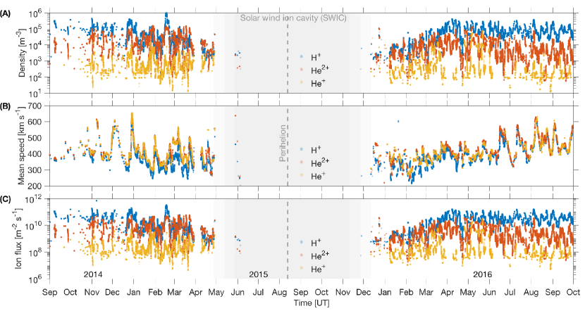
Figure 2: RPC-ICA-derived characteristics of the local solar wind ion distribution functions at comet 67P during the Rosetta mission (2014-2016) for H⁺, He²⁺ , and He⁺. (A) Density $n_{i}$, (B) mean ion speed $U_{i}$, and (C) ion flux $F_{i}$. The SWIC is approximately indicated as a gradually deeper gray region; its position with respect to the spacecraft is likely highly variable. All quantities have been submitted to a one-day moving average to remove variations due to the nucleus rotation. Increasingly intense colors indicate an increasing number of data points.

3.2 ROSINA-COPS

The Rosetta Orbiter Spectrometer for Ion and Neutral Analysis (ROSINA) is a suite of neutral and ion sensors (Balsiger et al., 2007). It consists of three instruments, one of which is the COmet Pressure Sensor (COPS), itself consisting of a nude and a ram gauge measuring the density and dynamic of the outflowing neutral gas, regardless of the composition (Bieler et al., 2015b). Another instrument of ROSINA is the Double Focusing Mass Spectrometer (DFMS): during the Rosetta mission, it measured the abundance of cometary volatiles (Fougere et al., 2016). By analyzing DFMS and COPS data with a 3D Monte Carlo direct simulation model, Hansen et al. (2016) developed an empirical model of the neutral coma; they also performed fits on the water production rate $Q_{0}$ for inbound (pre-perihelion) and outbound (post-perihelion) portions of the orbit around the Sun, corrected for seasonal effects (due to the changing latitude/longitude coverage of the spacecraft). Their finding is recalled here.

$$Q_{0}=\begin{cases}(2.58\pm 0.12)\times 10^{28}\ R_{\textnormal{Sun}}^{-5.10\pm 0.05}\ \textnormal{s}^{-1}\quad\text{inbound},\\ (1.58\pm 0.09)\times 10^{29}\ R_{\textnormal{Sun}}^{-7.15\pm 0.08}\ \textnormal{s}^{-1}\quad\text{outbound}.\end{cases}$$ (7)

Recently, Läuter et al. (2019) studied the temporal evolution of the H₂O, CO₂, CO, and O₂ neutral densities and outgassing rates using COPS and DFMS. In accordance with Fougere et al. (2016), they showed that H₂O dominated the neutral production in the coma during most of the mission, except after the post-perihelion equinox (March 2016, around $2.5$ AU), when CO₂ became the main outgassed species.

In the simple assumption of a spherically expanding cometary atmosphere (following Haser, 1957), the equivalent local outgassing rate inferred from ROSINA-COPS can be calculated as

$$Q_{\textnormal{ROS}} =4\pi\ \varv_{0}\ r^{2}\ n_{\textnormal{ROS}},$$ (8)

with $n_{\textnormal{ROS}}$ the neutral gauge density in m^-3 measured by ROSINA-COPS at the location of the spacecraft, $\varv_{0}$ the speed of the neutral gas in m s^-1, and $r$ Rosetta’s cometocentric distance in m. In the remaining study and for simplicity, we use the empirically determined analytical function of Hansen et al. (2016) to calculate the radial speed of the neutral gas $\varv_{0}$, in m s^-1:

$$\varv_{0} =\left(m_{R}R_{\textnormal{Sun}}+b_{R}\right)\ \left(1+0.171\ e^{-\frac{R_{\textnormal{Sun}}-1.24}{0.13}}\right),$$ (9)

$$\textnormal{with}\quad m_{R} =-55.5\quad\textnormal{and}\quad b_{R}=771.0,$$

where $m_{R}$ and $b_{R}$ are fitting parameters, and $R_{\textnormal{Sun}}$ is the heliocentric distance, expressed in AU.

The total ROSINA-COPS outgassing rate $Q_{\textnormal{ROS}}$, regardless of species involved, is shown in Fig. 5 (black line). The inbound/outbound fits of Hansen et al. (2016) are shown as an orange line in the same plot.

The total neutral column density $\eta$, empirical gas speeds $\varv_{0}$ , and outgassing rate $Q_{0}$ from ROSINA-COPS are shown in Fig. 3A and C throughout the Rosetta mission. To calculate $\eta$, we used Eq. (2), as in Beth et al. (2016). Periods when the spacecraft was in ”safe mode” ($1-10$ April 2016), as well as the two excursions at large cometocentric distance, one in late-September to mid-October 2015 (dayside excursion) and another in late-March to early-April (cometary tail excursion), are shown (Fig. 3B). These periods correspond to times when ROSINA measurements yielded large uncertainties or when the sensor was turned off. These periods are ignored in our interpretation. The column density varies by two orders of magnitude between perihelion ($1.24$ AU, $\eta\approx 2\times 10^{19}$ m^-2) and large heliocentric distances ($3$ AU, $\eta\approx 3\times 10^{17}$ m^-2), depending on Rosetta’s location at the comet throughout the mission. Oscillations in the column density, which for instance appear on a monthly basis after perihelion, are due to spacecraft latitudinal changes and different nucleus activities between the northern and southern hemispheres (see Heritier et al., 2018). Predictably, neutral speeds vary between about $550$ and $850$ m s^-1, and outgassing rates vary between about $10^{25}$ and $3\times 10^{28}$ s^-1, with maxima reached around perihelion.

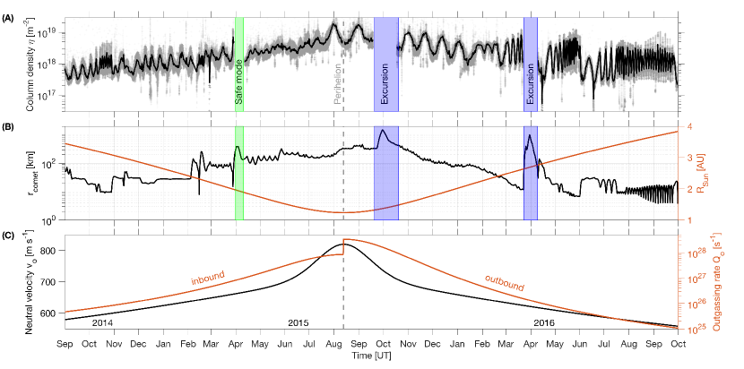
Figure 3: ROSINA-COPS-derived local neutral measurements at comet 67P during the Rosetta mission. (A) Time series of the local estimated ”upstream” column density of neutral species (gray crosses) from Eq. (2), and 24h moving-averaged values (black line). (B) Cometocentric distance of Rosetta (left), and heliocentric distance of comet 67P during the mission. (C) Empirically derived neutral outgassing speed (left axis) and outgassing rate (right axis) from Eqs. (9) and (7). Safe mode and excursions are indicated.

4 Results and discussion

The helium and hydrogen charge state distributions can be reconstructed using the analytical model presented in Paper II and based on the charge-changing and ionization cross section survey presented in Paper I. Such a reconstruction is used to help interpret the mission-wide ion spectrometer datasets. It was made in two steps: (i) the solar wind mean ion speed measured at the comet by RPC-ICA was used to derive the relevant energy-dependent cross sections throughout the mission, (ii) using the analytical model in forward or in inverse mode, the neutral outgassing rate and the upstream solar wind conditions may be successively inferred, and serve as tests of the validity of the model. Other interesting points, such as a summary of all ionization processes at the comet and an overview of the ENA environment of comet 67P can be derived, and are finally presented.

4.1 Local cross sections during the mission

In this study, charge-changing cross sections are presented for helium and hydrogen during the Rosetta mission. They are based on the careful survey made in Paper I and on our recommended velocity-dependent polynomial fits. We calculated the cross sections using the mean ion speed measured by RPC-ICA (Sect. 3.1 and Fig. 2B). For protons, we used $U_{\textnormal{sw}}(\textnormal{H}^{+})$. For all helium ions, we used for simplicity $U_{\textnormal{sw}}(\textnormal{He}^{2+})$, because $U_{\textnormal{sw}}(\textnormal{He}^{2+})$ and $U_{\textnormal{sw}}(\textnormal{He}^{+})$ have similar values and variations throughout the mission. The obtained charge-changing cross-section uncertainties varied with the charged state considered: they were $<25\%$ for He²⁺ and He⁺, but were $>75\%$ for He. Cross sections for hydrogen particles have large uncertainties on average, usually $>50\%$. For a thorough discussion of uncertainties and the reliability of the polynomial fits, we refer to Paper I.

Figure 4 shows the monochromatic charge-changing cross sections calculated at the mean speed of the solar wind, measured by RPC-ICA. Because no significant deceleration of the solar wind is seen in the RPC-ICA data throughout the mission, the thermal speed of the solar wind can be considered negligible with respect to the solar wind speed (equivalent to $T=0$ K).

Of all charge-changing processes, single-electron captures by He²⁺ and H⁺ have the largest cross section throughout the mission, with values $\gtrsim 10^{-19}$ m². For helium, two other processes have high cross sections ($\gtrsim 4\times 10^{-20}$ m²): the single-electron capture by He⁺ ($\sigma_{10}^{\textnormal{He}}$), and the double-electron capture of He²⁺ ($\sigma_{20}^{\textnormal{He}}$), especially between January 2015 and March 2016, when the heliocentric distance is shorter than $\sim 2.5$ AU. This results in the efficient conversion of He²⁺ ions into He ENAs. For hydrogen, the single-electron loss of H^- also has a large cross section, with $\sigma_{-10}^{\textnormal{H}}\approx 8\times 10^{-20}$ m², which is a factor of about $2$ lower than $\sigma_{10}^{\textnormal{H}}$. All other processes involving hydrogen particles have almost negligible cross sections in comparison; this preferentially creates H ENAs from solar wind protons, with these ENAs only undergoing a few losses to H⁺ or to H^-.

During most of the mission, solar wind ion speeds did not vary much, with an average speed around $400$ km s^-1, and they never dropped to below $250$ km s^-1. This implies that processes other than electron capture did not contribute much to changes in the charge state distribution. Consequently, when a Maxwellian-like solar wind is taken into account (with $T=40\times 10^{6}$ K for maximum effect, see Paper I and Paper II for a theoretical discussion), only minor changes are expected in the cross-section magnitudes, with the exception of ionization cross sections. In the following, we therefore only consider ”monochromatic” cross sections, and not Maxwellian-averaged cross sections, unless specified otherwise.

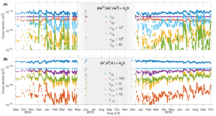
Figure 4: Monochromatic charge-changing cross sections during the Rosetta mission (2014-2016). (A) Helium species. (B) Hydrogen species. Cross sections are calculated using the mean solar wind ion speed of particles measured by RPC-ICA, with a solar wind temperature of $T=0$ K. A one-day moving average was performed for clarity. The solar wind ion cavity is indicated as a gray-shaded region.

4.2 Mission-wide inversions of Rosetta datasets

In this section, we present two inversions of the RPC-ICA datasets using our solar wind charge-changing analytical model. One results in the retrieval of the total cometary outgassing rate, the other in the reconstruction of solar wind upstream densities and fluxes.

4.2.1 Cometary outgassing rate

The inversion of our analytical model to retrieve the neutral outgassing rate from RPC-ICA ion flux data follows three steps: (i) calculation of $\mathcal{R}=F$(He⁺)/$F$(He²⁺) ion flux ratio measured by RPC-ICA locally, (ii) calculation of the geometrical quantity $\epsilon(r,\chi)=\chi/\left(4\pi\,\sin\chi\right)$ from the spacecraft position, and (iii) final inversion using expression (3) for $Q_{0}$. In this step, we assume that the atmosphere is solely composed of H₂O. Consequently, we adopt the velocity-dependent charge-changing cross sections in H₂O from Paper I, with solar wind speeds for hydrogen particles taken as $U_{i}=U_{\textnormal{H}^{+}}$ and for helium particles as $U_{i}=U_{\textnormal{He}^{2+}}$.

Figure 5A presents the local H₂O outgassing rate derived from in situ RPC-ICA measurements of ion flux ratios and compares it to those retrieved from ROSINA-COPS measurements using Eq. (8). We also superimpose the geometry-corrected fits of Hansen et al. (2016) for pre- and post-perihelion Rosetta datasets. For reference, the cometocentric and heliocentric distance variations are included in Fig. 5B.

For the ROSINA-COPS and RPC-ICA measurements, we performed $24$h moving averages to suppress variations due to the rotation of the cometary nucleus. Outgassing rates from ROSINA-COPS and from RPC-ICA are in very good agreement throughout the mission, and the neutral atmosphere variations are convincingly captured. On average, when a running average over 14 days is applied to study long-term trends, the RPC-ICA-derived rates are lower by a factor of about $1.3$ than those from ROSINA-COPS. Local differences between the two estimates may arise, for example, (i) from the ion dynamics and the increasing deflection and energy spread of solar wind ions, and (ii) from the assumption of a spherically symmetric outgassing used in this work. Such effects would need to be examined case by case and are therefore beyond the scope of this study. However, the improvement over past studies in the outgassing rate retrieval is clear; in comparison, using the simple inversion of Simon Wedlund et al. (2016) and Eq. (4) when one electron capture reaction is taken into account, the division factor stated above for 14-day running averages reaches about $1.8$ throughout the mission, in agreement with the results of Simon Wedlund et al. (2016). This indicates how relatively efficient other processes such as double-electron capture of He²⁺ and single-electron capture of He⁺ may become, depending on solar wind speed and cometocentric distance. Expression (5) for the outgassing rate, when no electron losses (no stripping reactions) are taken into account, most of the time yields results in between those from Eqs. (3) and (4): from January 2015 to June 2016, it remains within about $10\%$ of the full six-reaction model. Stripping reactions (especially $\sigma_{01}$ for He) are found to play an increasingly important role at large heliocentric distances (small cometocentric distances, at the validity limit of the model), where the no-electron-loss model produces outgassing rates that are on average $>30\%$ lower than the result of the full six-reaction model.

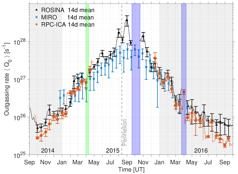
Figure 6: Local 14-day averaged water outgassing rate of comet 67P during the Rosetta mission (2014-2016) as measured by ROSINA-COPS (black line and triangles), MIRO (blue crosses, from Marshall et al., 2017), and retrieved from RPC-ICA (red line and circles, tabulated in Table 1). Error bars correspond to the median absolute standard deviations. Colored regions denote spacecraft excursions and safe modes, as in Fig. 5.

To examine the long-term trends of our retrievals in detail, the 14-day moving average of the RPC-ICA-derived local H₂O outgassing rates, $\langle Q_{0}\rangle$, is tabulated in Table 1 and plotted in Fig. 6. Strong fluctuations of the measured RPC-ICA signal result in large standard deviations that at times exceed $30\%$. We compare these rates to the $14$-day moving averages of the local H₂O outgassing rates of Marshall et al. (2017) (see their Table 1) using the Microwave Instrument for the Rosetta Orbiter (MIRO): these averages have errors larger than $30\%$ at large cometocentric distances and reach about $50\%$ at perihelion. The RPC-ICA rates compare well with those of MIRO in their common temporal coverage, as well as with those of ROSINA-COPS (black triangles in the figure). At large heliocentric distances, especially after July 2016 (post-perihelion), large differences between ROSINA-COPS and RPC-ICA can be seen: they coincide with Rosetta’s increasingly deep dips into the inner cometary atmosphere around and below $10$ km cometocentric distance. As recalled in Sect. 2, this distance corresponds to the lower validity limit of the analytical model, and may at those times explain in part the poor quality of our outgassing rate retrieval.

Table 1: Local water outgassing rates $\langle Q_{0}\rangle$ derived from RPC-ICA charge-exchange analysis of solar wind ion fluxes, with a $14$-day moving average applied to the full dataset, as shown in Fig. 6. $R_{\mathrm{Sun}}$ is the heliocentric distance.

Date	Heliocentric distance	Local average outgassing rate
[UT]	$R_{\mathrm{Sun}}$ [AU]	$\langle Q_{0}\rangle$ [$\times 10^{26}$ s-1]
	Pre-perihelion
01-10-2014	3.26	$0.28\pm 0.02$
15-10-2014	3.16	$0.32\pm 0.10$
01-11-2014	3.06	$0.40\pm 0.10$
15-11-2014	2.96	$0.65\pm 0.20$
01-12-2014	2.86	$1.00\pm 0.21$
15-12-2014	2.75	$0.86\pm 0.19$
01-01-2015	2.65	$1.30\pm 0.39$
15-01-2015	2.54	$1.20\pm 0.19$
01-02-2015	2.42	$4.30\pm 0.66$
15-02-2015	2.31	$4.80\pm 0.70$
01-03-2015	2.21	$5.70\pm 0.64$
15-03-2015	2.10	$8.50\pm 1.00$
01-04-2015	1.99	$8.00\pm 2.10$
15-04-2015	1.85	$17.00\pm 5.00$
	Post-perihelion
15-12-2015	1.91	$36.00\pm 15.00$
01-01-2016	2.01	$14.00\pm 2.70$
15-01-2016	2.12	$8.30\pm 1.70$
01-02-2016	2.25	$12.00\pm 1.90$
15-02-2016	2.37	$5.60\pm 1.10$
01-03-2016	2.48	$2.10\pm 0.42$
15-03-2016	2.58	$2.10\pm 0.77$
01-04-2016	2.70	$4.60\pm 0.67$
15-04-2016	2.80	$0.96\pm 0.16$
01-05-2016	2.91	$1.30\pm 0.43$
15-05-2016	3.00	$0.81\pm 0.49$
01-06-2016	3.12	$0.76\pm 0.23$
01-07-2016	3.30	$0.30\pm 0.02$
15-07-2016	3.39	$0.72\pm 0.15$
01-08-2016	3.50	$0.32\pm 0.06$
15-08-2016	3.58	$0.26\pm 0.06$
01-09-2016	3.67	$0.18\pm 0.02$
15-09-2016	3.75	$0.27\pm 0.04$

Other sources of errors in our retrievals are present. The charge-changing cross-section uncertainties are usually larger than $25\%$ (see Paper I); propagating these uncertainties in the model would result in different outgassing rate retrievals. Because of the number of involved cross sections and associated errors, and because of fluctuations in the RPC-ICA moment-derived fluxes in the first place, outgassing rate retrievals may change by an estimated $50\%$. This is arguably much less than the daily fluctuations of the signal, which can reach $>100\%$ because of varying solar wind and plasma conditions encountered at the comet.

We described above that although CO₂ becomes the main neutral cometary species after March 2016, the retrieval of the total outgassing rate from RPC-ICA is in rather good agreement with that of ROSINA-COPS until the end of the mission, with an underestimation of the RPC-ICA outgassing rate after July 2016. Because charge-changing cross sections in H₂O and CO₂ only differ by a factor $2$ at most, this underestimate can thus be ascribed to at least two supplementary factors: (i) the changing composition of the atmosphere, and (ii) the fast-varying column densities encountered by Rosetta at that time (see Fig. 3A).

Least-square fits of the form $\alpha\,R_{\textnormal{Sun}}^{-\beta}$ were performed on the one-day averaged RPC-ICA data, with the following results:

$$Q_{\textnormal{ICA}}=\begin{cases}(1.16\pm 0.04)\times 10^{29}\ R_{\textnormal{Sun}}^{-7.00\pm 0.03}\ \textnormal{s}^{-1}\quad\text{inbound},\\ (7.21\pm 0.14)\times 10^{28}\ R_{\textnormal{Sun}}^{-6.29\pm 0.02}\ \textnormal{s}^{-1}\quad\text{outbound}.\end{cases}$$ (10)

The errors correspond to the mean one-day variations of the signal and therefore do not include the instrument uncertainty. These fits are shown in Fig. 5 (blue lines). At perihelion, our inbound and outbound fits connect rather well, with only a slight discontinuity. Although on average these fits do bear similarities with the season-corrected fits of Hansen et al. (2016), they do differ, predominantly outside of times when observations from RPC-ICA and ROSINA-COPS were simultaneously available, which is expected. Except for the temporal coverage, one main difference is that Hansen et al. (2016) first corrected the ROSINA-COPS data for seasonal effects by applying their DSMC model before they performed the fits. Our approach is much simplified in comparison, as only $24$-hour means (almost two nucleus rotations) were made on the RPC-ICA data before the fits were performing. For the later part of the mission (after the second large-distance excursion), our fits are arguably in better agreement with ROSINA-COPS data than the empirical fits of Hansen et al. (2016): the reason is that the post-excursion observations were not yet available at the time of publication of the Hansen et al. (2016) study. A reverse conclusion holds for example in the early stages of the mission (before October 2014), when RPC-ICA could not detect He⁺ ions because of poor temporal coverage due to instrument problems (Nilsson et al., 2015a, 2017). In that period, our fit therefore substantially underestimates the measured ROSINA-COPS outgassing, which is better captured by the model of Hansen et al. (2016).

We note that our inbound fit parameterization is coincidentally very close to the value determined by Simon Wedlund et al. (2016) ($1.14\times 10^{29}\,R_{\textnormal{Sun}}^{-7.06}$), where events were manually selected and particle fluxes were energy-summed individually (instead of calculating the moments of the ion distribution functions), and where only one charge-exchange reaction was used to invert the particle flux ratios. When this one-reaction simplification is applied to our current moment-based dataset, the fit becomes $Q_{0}=1.39\times 10^{29}\,R_{\textnormal{Sun}}^{-7.58}$ for the inbound leg, which is a factor $1.5$ to $2$ lower for $R_{\textnormal{Sun}}>2.5$ AU (when Rosetta orbited at cometocentric distances smaller $50$ km) than our current estimate with the full analytical six-reaction model. A similar conclusion befits the outbound leg data, for which the simple one-reaction model yields $Q_{0}=1.58\times 10^{29}\,R_{\textnormal{Sun}}^{-7.44}$ (factor $1.4$ to $2.2$ lower for $R_{\textnormal{Sun}}>2.5$ AU), which is caused by the progressively closer probing of Rosetta to the nucleus after May 2016. In agreement with Paper II, this result indicates that other processes than single-electron capture by He²⁺ became more and more important at orbits that lay deeper inside the coma.

Obtaining a lower limit estimate of the outgassing rate is, in principle, possible by studying the appropriate ion cyclotron wave (ICW) activity at the comet with the use of a magnetometer, as demonstrated by Huddleston et al. (1998) and Volwerk et al. (2001, 2013b, 2013a). Such a magnetometer is present on board Rosetta as part of the Rosetta Plasma Consortium, the RPC-MAG fluxgate magnetometer (Glassmeier et al., 2007). Because of the low-frequency nature of these waves, $5\times 10^{-3}\leavevmode\nobreak\ \leq\leavevmode\nobreak\ f_{\rm c,H2O}\leavevmode\nobreak\ \sim\leavevmode\nobreak\ 2\times 10^{-2}$ Hz and the strong compressional wave power, detection is difficult. A detailed study is currently under way.

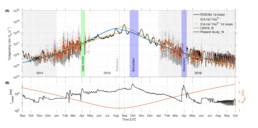
Figure 5: (A) Local water outgassing rate of comet 67P during the Rosetta mission (2014-2016), as measured by ROSINA (black line, one-day moving average) and retrieved from RPC-ICA. RPC-ICA one-day moving averages are presented as red circles, whereas the full non-averaged time series is shown as gray pluses. Safe mode and excursions are indicated: at these dates, the outgassing rate from ROSINA-COPS yields unreliable results. Inbound and outbound fits to the ROSINA data of Hansen et al. (2016) (orange line, corrected for latitude/longitude effects) and to the RPC-ICA data (blue line, this study) are shown. (B) Cometocentric (left axis) and heliocentric distances (right axis) during the mission. Instrumental uncertainties are estimated to be $15\%$ for ROSINA-COPS.

4.2.2 Upstream solar wind

As discussed in Paper II, SWCX is responsible for the conversion of upstream solar wind He²⁺ ions into a mixture of He²⁺, He⁺ , and He⁰ particles: this is expected to result in the local decrease of solar wind He²⁺ ion fluxes measured deep in the cometary coma. The question now is to quantify this decrease. In Sect. 2 we recalled that it is possible to retrieve the upstream solar wind fluxes from local RPC-ICA measurements of H⁺ and He²⁺ fluxes. For this purpose, we inverted the analytical model and used Eq. (6). To be consistent in our approach, we used as inputs the locally measured He²⁺ fluxes, the RPC-ICA-derived outgassing rates retrieved in the previous section, and the neutral velocity reported by Hansen et al. (2016).

Figure 7A presents the results of the inversion for He²⁺ ions measured by RPC-ICA in the inner coma. We compared our retrieved solar wind He²⁺ particle flux, $F^{\textnormal{sw}}_{\alpha}$ with measurements made at Earth (by the satellites ACE an WIND) and at Mars (by the satellite Mars Express, or MEX), and time- and angle-propagated to the position of comet 67P, assuming a simple Parker-spiral ballistic propagation model (for details, see Behar, 2018). The ion spectrometer ASPERA-3 IMA on board MEX (Barabash et al., 2006) that we used here was built by the same institute as that of RPC-ICA: thus, both spectrometers are almost identical. ACE measurements (from the Solar Wind Electron, Proton, and Alpha Monitor, SWEPAM electrostatic analyzer) were obtained from the ACE Science Center (McComas et al., 1998). In the figure, we plot the daily average for clarity, combining MEX and ACE data. We conservatively assumed that the solar wind contained about $4\%$ of He²⁺ ions (Slavin & Holzer, 1981), and hence the proton flux $F^{\textnormal{sw}}_{p}$ measured by ACE and MEX is $F^{\textnormal{sw}}_{\alpha}=\nicefrac{{1}}{{24}}\,F^{\textnormal{sw}}_{p}$.

Despite strong fluctuations in the cometary data, the daily averages from RPC-ICA and MEX-ACE are in relatively good agreement throughout the mission, until about April 2015, and after February 2016. As pointed out earlier, a clear decrease in flux is seen at these times in the local RPC-ICA data (black line in Fig. 7). According to our model calculations, this cannot be explained by an increased efficiency of charge-changing reactions: the retrieved upstream particle flux (red line) is only marginally higher than the local flux during these periods, with an increase of a factor of $2$ on average, which is far different from the expected fluxes from MEX-ACE. We note, however, that this efficiency level of charge-changing reactions is in agreement with the conclusions reached in Paper II for a synthetic test case applied to Rosetta: SWCX effects were mostly expected around perihelion, when the neutral density reached sufficiently high levels (see also Appendix B of Paper II on charge-exchange collision depth).

The discrepancy may stem from at least two immediate issues that we describe below.

• Instrumental bias. The RPC-ICA field of view is only about $2.8\pi$ sr, therefore the instrument may have missed several detections of ions, which may have led to an underestimation of the local solar wind ion flux. This in turn would lead in the model to an underestimation of the upstream solar wind flux, especially since the latter is derived from He²⁺ local fluxes alone. When we used He⁺ ions to derive the upstream solar wind He²⁺ flux, differences of up to a factor $2-5$ between the two retrievals were obtained, which points to the problem of defining the initial conditions in the model. When the outgassing rate was derived (previous section), this problem was circumvented by the use of a ratio of ion fluxes.

• Model bias. In the model, the dynamics of solar wind ions is not self-consistently taken into account: for instance, their cycloidal paths and observed deflection (Behar et al., 2017) may substantially increase the path of the ions in the atmosphere, and hence the total column density traversed. When we multiply by $4$ the path traversed by the ions, as may be expected from half an arc length in a typical cycloidal motion, we witness a dramatic increase in the retrieved ion flux below $2.5$ AU that reaches up to a factor $10$ and matches the levels expected from MEX-ACE measurements.

Moreover, the model does not assume any formation of boundaries upstream of the nucleus, contrary to observational evidence (Gunell et al., 2018). Following Paper II, we investigated the effect of high Maxwellian temperatures, that is, $T\leavevmode\nobreak\ =\leavevmode\nobreak\ 40$ MK ($\varv_{\textnormal{th}}\,=\,500$ km s^-1), on the retrieval of upstream solar wind fluxes. Differences of less than $10\%$ between the two retrieved fluxes were found, in agreement with the findings of Paper II, which is marginal in comparison to geometrical effects (e.g., the path length). In Fig. 7B the solar wind ions measured by RPC-ICA do not display any significant slowing-down throughout the mission: they are in good agreement with ACE/MEX upstream measurements, with only an indication of a $50$ km s^-1 deceleration from December 2015 to February 2016. This decrease in speed is small enough to affect the cross section values very little (see Paper I). Consequently, the current balance between all cross sections is expected to remain mostly unaffected. For example, an increase in double-electron capture cross sections for He²⁺ would be expected if solar wind single particle speeds were to drop below $200$ km s^-1, which was never the case during the mission.

The main discrepancy between upstream-retrieved and Rosetta-propagated fluxes requires further investigation at this stage. It would also benefit from the use of self-consistent models such as hybrid models (Koenders et al., 2016; Simon Wedlund et al., 2017). This is left for a future study.

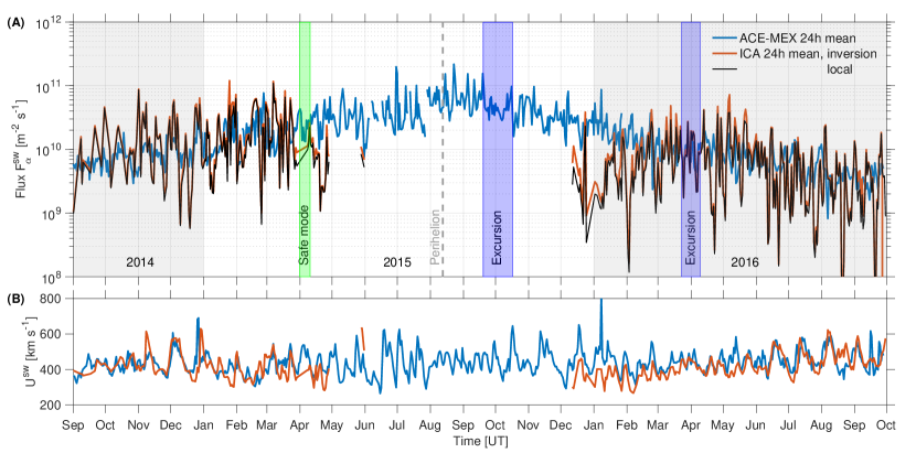
Figure 7: Upstream ’undisturbed’ and locally measured solar wind parameters during the Rosetta mission (2014-2016), averaged over one day. (A) Solar wind He²⁺ flux, noted $F^{\textnormal{sw}}_{\alpha}$, from ACE-MEX (blue line), and retrieved from RPC-ICA local measurements at comet 67P (red line). Local RPC-ICA fluxes are shown in black for comparison. (B) Solar wind speed measured by ACE-Mars Express (H⁺, blue line) and by RPC-ICA (He²⁺, red line).

4.3 Ionization processes at comet 67P

Heritier et al. (2018) compared photoionization (PI) frequencies with electron-impact ionization (EI) frequencies, showing that EI played a major role at large heliocentric distances ($>2.8$ AU) in the creation of new plasma. Although charge-transfer reactions may not always result in the net creation of ions, they contribute nonetheless to the general ionization of the coma by adding heavy cometary ions to the cometary plasma. Moreover, solar wind ions are also capable of ionizing the neutral cometary atmosphere to produce new ions due to their high kinetic energies.

We present in this section the in situ ionization frequency due to SWCX and solar wind impact ionization (SWI), and compare them to PI and EI rates. The results of Heritier et al. (2018) (see their Fig. $16$) for the PI and EI frequencies are reproduced in Fig. 8 with a brief summary below. PI frequencies for an H₂O coma at the location of Rosetta were estimated from the daily EUV solar fluxes measured at Earth by the Thermosphere Ionosphere Mesosphere Energetics and Dynamics-Solar EUV experiment (TIMED-SEE, Woods et al., 2005), phase- and time-shifted to the position of comet 67P and scaled to its heliocentric distance ($\propto 1/R_{\textnormal{Sun}}^{2}$). EI frequencies were calculated using electron fluxes above about $12.5$ eV from the Rosetta Ion and Electron Sensor (RPC-IES, Burch et al., 2007). Daily standard deviations are given in Heritier et al. (2018).

The SWCX and SWI processes were calculated locally from RPC-ICA solar wind ion particle fluxes $F_{i}$ (units of m^-2 s^-1), with subscript $i=p$, $i=\alpha$, and $i=\textnormal{He}^{+}$ for H⁺, He²⁺ , and He⁺, respectively. The total SWCX frequencies $\sum_{i}f^{\textnormal{swcx}}_{i}$ expressed in s^-1 are thus

$$f^{\textnormal{swcx}}_{\textnormal{tot}} =f^{\textnormal{swcx}}_{p}+f^{\textnormal{swcx}}_{\alpha}+f^{\textnormal{swcx}}_{\textnormal{He}^{+}},$$ (11)

with

$$\begin{cases}f^{\textnormal{swcx}}_{p}=\left(\sigma_{10}(U_{p})+\sigma_{1-1}(U_{p})\right)\ F_{p}\\ f^{\textnormal{swcx}}_{\alpha}=\left(\sigma_{21}(U_{\alpha})+\sigma_{20}(U_{\alpha})\right)\ F_{\alpha}\quad.\\ f^{\textnormal{swcx}}_{\textnormal{He}^{+}}=\sigma_{10}(U_{\textnormal{He}^{+}})\ F_{\textnormal{He}^{+}}\end{cases}$$

Hydrogen and helium cross sections $\sigma_{ij}$ were taken at the ion speed $U_{i}$ measured by RPC-ICA. Similarly, the total solar wind impact ionization frequencies $\sum_{i}f^{\textnormal{swi}}_{i}$ in s^-1 were calculated as

$$f^{\textnormal{swi}}_{\textnormal{tot}} =f^{\textnormal{swi}}_{p}+f^{\textnormal{swi}}_{\alpha}+f^{\textnormal{swi}}_{\textnormal{He}^{+}},$$ (12)

with

$$\begin{cases}f^{\textnormal{swi}}_{p}=\sigma_{11}(U_{p})\ F_{p}\\ f^{\textnormal{swi}}_{\alpha}=\sigma_{22}(U_{\alpha})\ F_{\alpha}\quad.\\ f^{\textnormal{swi}}_{\textnormal{He}^{+}}=\sigma_{11}(U_{\textnormal{He}^{+}})\ F_{\textnormal{He}^{+}}\end{cases}$$

For ionization by protons and $\alpha$ particles, the average energy of the ejected electrons at solar wind energies is expected to be about $5$ eV (Uehara et al., 2000; Uehara & Nikjoo, 2002).

Figure 8 presents a comparison of all ionization channels at comet 67P, assuming only water as neutral constituent of the coma: daily averaged PI (gray line) and EI (pink circles), as well as non-averaged SWCX (blue) and SWI (red). Daily averaged SWCX and SWI frequencies are plotted as black lines overlaid on the non-averaged data; this demonstrates the extreme variability of fluxes measured at Rosetta during the mission. During the early mission and toward its end, electron ionization often becomes the largest contribution (Galand et al., 2016; Heritier et al., 2018) that even exceeds PI, whereas PI remains dominant in the so-called solar wind ion cavity between May and December 2015.

On average, SWCX is a factor $5$ lower than PI at large heliocentric distances (early and late mission, coinciding with cometocentric distances $<50$ km, see Fig. 5B). After January 2015 ($R_{\textnormal{Sun}}<2.8$ AU), this factor reaches $10$ on average, until the substantial drop in solar wind flux after March 2015 ($R_{\textnormal{Sun}}<2.4$ AU), where SWCX becomes $100$ times less efficient than PI. A similar trend is seen for the outbound leg, with an average factor $5$ between PI and SWCX reached after April 2016 ($R_{\textnormal{Sun}}>2.8$ AU). This heliocentric distance coincides on the inbound and outbound legs with the sudden drop in solar wind ion fluxes, a prelude to the formation of the solar wind ion cavity (Behar et al., 2017).

Occasionally, SWCX ionization frequencies can become higher than PI frequencies and rival EI rates, as is the case in November 2014, at the end of February 2015, and frequently toward the end of the mission. This is the result of increased fluxes that may be related to solar wind transient events such as interplanetary coronal mass ejections (ICMEs) or corotating interaction regions (CIRs). The October-November 2014 SWCX frequency increases coincide for example with the occurrence of several CIRs, as described in Edberg et al. (2016). Similarly, Hajra et al. (2018) studied CIR events between June and September 2016: their impact at the comet correlated relatively well with sudden increases in charge-exchange rates; the authors used the same calculation method as presented here. Because of the large daily variations in the flux, however, case-by-case studies must be performed to study in more detail how SWCX rates compare with EI.

Throughout the mission, SWI is a constant $50$ times lower than SWCX, which makes it a negligible plasma source in comparison to ionization by electron impact and solar EUV radiation. This is stemming from ionization cross sections, which peak at velocities above $1000$ km s^-1, and are thus small in the typical solar wind velocity ranges (see Paper I for details). However, this assessment may change if the solar wind is substantially heated, as would be expected with the formation of boundaries and bow shock-like structures upstream. For example, as shown in Paper I, total proton ionization cross sections may be multiplied by about a factor $10$ at $400$ km s^-1 solar wind speed: such an increase in SWI cross sections would significantly narrow the gap with the SWCX frequency. However, in order to match the levels of PI, an even larger increase in cross section would be necessary (e.g., a factor $100-500$), which may occur for a significant slowing-down of the solar wind (below $200$ km s^-1). Although this condition is not met at comet 67P during the Rosetta mission, such a large deceleration is expected at high-activity comets such as comet 1P/Halley.

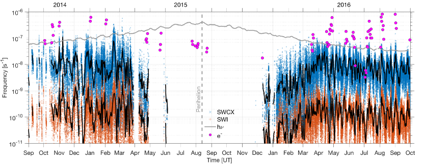
Figure 8: Local ionization production frequencies at comet 67P during the Rosetta mission (2014-2016). The contribution of SWCX (blue line), SWI (red lines), PI or $(h\nu$, $24$h average, gray line), and EI (or $e^{-}$, $24$h average, pink circles) to the local production of ions is displayed. The black continuous lines are the $24$h averaged SWCX and SWI frequencies. When Rosetta was inside the solar wind ion cavity (May-December 2015), no solar wind fluxes could be routinely measured.

4.4 ENA environment: predictions from RPC-ICA data

From SWCX reactions, ENAs such as He⁰ and H⁰ can be efficiently produced. Our analytical model of charge-changing processes at the comet is able to reproduce their distribution throughout the Rosetta mission (see also Paper II) using He⁺-to-He²⁺ particle flux ratios to calibrate our model to the observations. For inputs, we used here cross sections at the mean speed of the solar wind measured by RPC-ICA, the column density derived from ROSINA, and, as previously, the neutral outgassing velocity from the Hansen et al. (2016) empirical formula.

Figure 9A shows first the reconstructed in situ He⁺/He²⁺ particle flux ratios (in blue, noted $\mathcal{R}_{\textnormal{He}^{+}}$ in the following) as compared to those measured locally by RPC-ICA (in black). Excellent agreement between the two curves is achieved throughout the mission, which a posteriori is another confirmation of the accuracy of the outgassing retrieval performed in Section 4.2.1 when the RPC-ICA flux ratio is used to estimate it. This enables us to derive with confidence the corresponding local flux ratio for the production of helium ENAs He⁰/He²⁺, noted $\mathcal{R}_{\textnormal{He}}$. At the beginning of the mission, the ENA He⁰ flux at Rosetta is expected to be about a factor $2$ lower than that of He⁺. When the He⁺ flux starts to drop in March 2015 (see Fig. 2), this factor is closer to one, meaning that in the denser atmosphere of this time period, there would be as many He⁺ ions than He ENAs at Rosetta’s location. The tendency is identical after perihelion for the outbound leg, where ENAs and He⁺ ions are in the same proportion in the solar wind plasma until March 2016. After this, He⁺ ion fluxes routinely become $2-3$ times as high as He ENAs. In extremely rare events, we predict that ENAs can come to $50\%$ of He²⁺ and dominate over He⁺ ions: this occurs once on 24 April 2015, and after perihelion on 12 and 31 December 2015, and on 6-7 February 2016. A detailed study of such events is beyond the scope of this paper, but may be tentatively linked to sudden changes in the upstream solar wind plasma, driven by solar transients such as CIRs (Hajra et al., 2018).

We calculated the ENA ratio for hydrogen and show it in Fig. 9B. Because of high proton fluxes outside of the solar wind ion cavity, the proportion of H ENAs is expectedly large throughout the mission; the ENA flux may even become higher than the proton flux in very rare events (ratio above $1$, as in February and March 2015, and after perihelion in December 2015, occasionally in January and February 2016, and large periods of time in March and May 2016). The highest predicted ENA fluxes are immediately after Rosetta exited the SWIC. Correspondingly, the proportion of H^- negative ions is predicted to be no more than $0.01\%$ of the proton flux throughout most of the mission, reaching higher levels in the same transient events as for H ENAs.

These ratios can in turn be used to predict the total fluxes of ENAs that could have been measured had Rosetta included an ENA detector. For helium ENAs,

$$F_{\textnormal{He}} =\mathcal{R}_{\textnormal{He}}\ F_{\alpha}^{\textnormal{ica}}=\frac{\mathcal{R}_{\textnormal{He}}}{\mathcal{R}_{\textnormal{He}^{+}}^{\textnormal{ica}}}F_{\textnormal{He}^{+}}^{\textnormal{ica}},$$ (13)

$$\textnormal{with}\quad\mathcal{R}_{\textnormal{He}}=\frac{F_{\textnormal{He}}}{F_{\alpha}}\quad\textnormal{and}\quad\mathcal{R}_{\textnormal{He}^{+}}^{\textnormal{ica}}=\frac{F_{\textnormal{He}^{+}}}{F_{\alpha}}.$$

Ion fluxes for He²⁺ and He⁺, noted $F_{\alpha}^{\textnormal{ica}}$ and $F_{\textnormal{He}^{+}}^{\textnormal{ica}}$, and the particle flux ratio $\mathcal{R}_{\textnormal{He}^{+}}^{\textnormal{ica}}$ are here measured by RPC-ICA, whereas the ratio $\mathcal{R}_{\textnormal{He}}$ is calculated in Fig. 9 by the analytical model, using ROSINA-COPS data for the neutral atmosphere. To better constrain the model with the flux ratio $\mathcal{R}_{\textnormal{He}^{+}}$ measured by RPC-ICA (in an attempt to ignore fluctuating upstream solar wind conditions), we chose the second expression in Eq. (13), which multiplies the ratio of flux ratios by the measured He⁺ flux, acting as a calibration factor for the model.

For hydrogen ENAs and negative ions H^-, a similar development yields

$$F_{\textnormal{H}} =\mathcal{R}_{\textnormal{H}}\ F_{p}^{\textnormal{ica}},$$ (14)

$$F_{\textnormal{H}^{-}} =\mathcal{R}_{\textnormal{H}^{-}}\ F_{p}^{\textnormal{ica}},$$ (15)

with $$\quad\mathcal{R}_{\textnormal{H}}=\frac{F_{\textnormal{H}}}{F_{p}}\quad\textnormal{and}\quad\mathcal{R}_{\textnormal{H}^{-}}=\frac{F_{\textnormal{H}^{-}}}{F_{p}},$$

with $F_{p}^{\textnormal{ica}}$ the flux of protons measured by RPC-ICA. All other quantities were calculated by the model.

Figures 10A and B present the synoptic summary of daily averaged fluxes of solar wind origin at comet 67P at the position of Rosetta. He²⁺, He⁺, and H⁺ fluxes are all measured by RPC-ICA, whereas all other particles fluxes are predicted by the model. We note, as before, that He⁺ and He ENAs have similar levels throughout the mission, with occasional spikes in magnitude that propel them to the levels of He²⁺ ions. This suggests that most of the time, Rosetta orbited at a cometocentric distance where He⁺ and He⁰ charge states were equally distributed (see Paper II for cometocentric profiles).

Regarding hydrogen particles, it is clear from Fig. 10B that H ENAs and protons have similar flux levels throughout the mission, except at its very beginning, and, marginally, at its very end. Possible effects of an increased ENA environment are discussed in Ip (1990) for comet 1P/Halley and include heating of the cometary ions. H^- anions have very low fluxes throughout the mission; despite this, Burch et al. (2015) found evidence of H^- in the early RPC-IES datasets, which persisted up to January 2015. Our model predicts the most favorable detection conditions for H^- in December 2015, around mid-March 2016 and in May 2016. This would need to be investigated further with RPC-IES: flux ratios could give an indication of charge-exchange efficiencies, which could easily be compared with our model to RPC-IES and RPC-ICA datasets for helium.

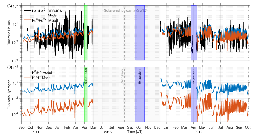
Figure 9: Particle flux ratios during the Rosetta mission 2014-2016. (A) Helium species. The 1h averaged He⁺/He²⁺ ratio measured by RPC-ICA (black) is compared to the daily averaged analytical forward model solution (blue), with mean speed $U_{\textnormal{sw}}=U_{\textnormal{ICA}}$(He²⁺). The column density is derived from ROSINA data. Modeled He⁰/He²⁺ flux ratios are shown in red. (B) Hydrogen species, with modeled H⁰/H⁺ (blue) and H^-/H⁺ (red) ratios for a solar wind mean speed $U_{\textnormal{sw}}=U_{\textnormal{ICA}}$(H⁺). The solar wind ion cavity is indicated as a gradually denser gray-shaded region. Safe mode and excursions where ROSINA data were excluded from the analysis are indicated.

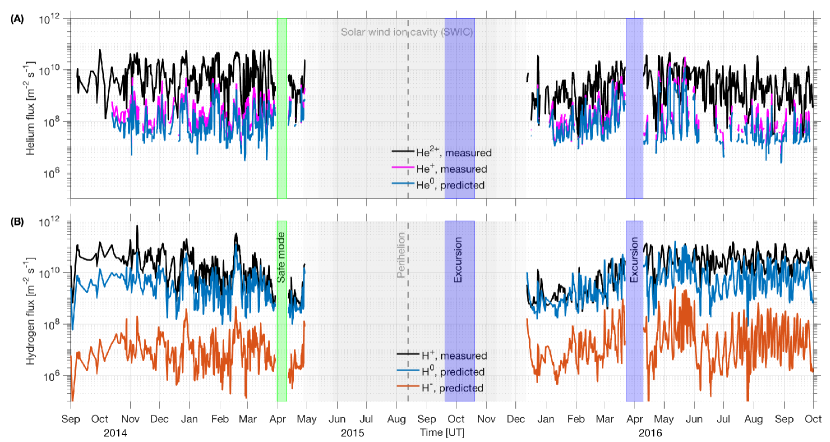
Figure 10: Solar wind ion and ENA fluxes during the Rosetta mission 2014-2016. The fluxes are measured when available by RPC-ICA, and when unavailable, are predicted by the analytical model using ROSINA-COPS and RPC-ICA data. All fluxes are averaged over $24$ h. (A) Helium species. (B) Hydrogen species. ENA fluxes are drawn in blue for clarity. The solar wind ion cavity is indicated as a gray-shaded region. Safe mode and excursions where ROSINA data were excluded from the analysis are indicated.

5 Conclusions

This study is the culmination of our investigation of charge-changing reactions in cometary atmospheres. Simon Wedlund et al. (2019b) (Paper I) made a careful survey of available velocity-dependent charge-changing and ionization cross sections in H₂O. Simon Wedlund et al. (2019a) (Paper II) developed a new analytical model of charge-changing reactions in comets based on these cross sections, with a systematic exploration of the parameter space (heliocentric and cometocentric distances) of our simulations. In this study, we have applied this model to the complex datasets of the cornerstone ESA-Rosetta mission to comet 67P/Churyumov-Gerasimenko. We have provided mission-wide interpretations of the RPC-ICA ion spectrometer data and attempted to place them in the larger context of cometary plasma physics. More specifically, we have shown the following.

1. Single-electron and double-electron capture cross sections dominate for H⁺ and He²⁺ solar wind ions interacting with a H₂O 67P-like coma. Electron stripping may have played a role at 67P for large heliocentric and small cometocentric distances.

2. Remote sensing of the cometary neutral atmosphere from local ion measurements is possible. Outgassing rates derived from the local He⁺/He²⁺ flux ratio were well within a factor $2$ of the neutral pressure sensor estimates: 14-day averages between January 2015 and June 2016 were within $10\%$ of each other and the MIRO estimates. Our fitted production rates agree well with those of Hansen et al. (2016).

3. Solar wind upstream retrievals from local ion measurements are difficult, especially for high solar wind ion deflections when closing in on the SWIC. The model was not able to explain the sharp drop in flux in this region, which may either indicate that other mechanisms are at work or that our current approach has problems in taking charge exchange into account. The latter may stem from limiting assumptions in the analytical model (e.g., it does not take the dynamics of individual ions into account), and possibly from RPC-ICA missing detecting ions in the pre-SWIC region. It is not known at this stage if an additional constraint on the observed downstream fluxes would yield a better estimate in the model.

4. Charge-exchange reactions play an important role in the inner coma of comet 67P. A comparative summary of all ionization processes, PI, EI, SWCX, and SWI during the Rosetta mission was presented. We identified periods when SWCX may for a short time rival electron ionization frequencies in the production of ions. Throughout the mission, SWI played only a minor role, except when significant solar wind heating and strong deceleration of the solar wind flow were concomitantly present; these conditions may be best simultaneously fulfilled for high-activity comets such as comet 1P/Halley.

5. Hydrogen and helium ENAs are expected to play an important role in the inner coma, with modeled fluxes predicted to match and occasionally even exceed the levels of protons and $\alpha$ particles during the Rosetta mission. Enhanced ENA fluxes may in turn lead to localized heating in the coma.

Our approach may be improved in two main directions. On the one hand, the model inputs could be better constrained: a better determination of charge-changing cross sections or a complementary use of truly 3D ion and ENA measurements to determine the flux ratios would help decrease the errors in the retrievals. On the other hand, improvements on the physics of the model are clearly possible, but would come at the expense of the simplicity and portability of our initial approach: they include the addition of a realistic solar wind ion dynamics (gyromotion and deflection), or that of a more realistic neutral atmosphere (asymmetric outgassing), for example.

As it stands, our analytical model may readily be coupled with test particle simulations using electromagnetic fields calculated by hybrid models to investigate the charge-state distribution of ions in a cometary atmosphere. As a simple tool to interpret usually complex datasets, it can also deliver charge-exchange diagnoses in a wide variety of environments, ranging from astrophysical environments (interstellar medium, etc.) to planetary atmospheres.