On non-linear Schrödinger equations for open quantum systems

Abstract

Recently two generalized nonlinear Schrödinger equations have been proposed by Chavanis [Eur. Phys. J. Plus 132 (2017) 286] by applying Nottale’s theory of scale relativity relying on a fractal space-time to describe dissipation in quantum systems. Several existing nonlinear equations are then derived and discussed in this context leading to a continuity equation with an extra source/sink term which violates Ehrenfest theorem. An extension to describe stochastic dynamics is also carried out by including thermal fluctuations or noise of the environment. These two generalized nonlinear equations are analyzed within the Bohmian mechanics framework to describe the corresponding dissipative and stochastic dynamics in terms of quantum trajectories. Several applications of this second generalized equation which can be considered as a generalized Kostin equation have been carried out. The first application consists of the study of the position-momentum uncertainty principle in a dissiaptive dynamics. After, the so-called Brownian-Bohmian motion is investigated by calculating classical and quantum diffusion coefficients. And as a third example, transmission through a transient (time dependent) parabolic repeller is studied where the interesting phenomenon of early arrival is observed even in the stochastic dynamics although the magnitude of early arrival is reduced by friction.

I Introduction

Since perfect isolation of quantum systems is not possible, any realistic quantum system is influenced by its environment. By taking into account the interaction of the system with its environment, the corresponding dynamics becomes stochastic. There are three main approaches in the literature to study dissipative and stochastic effects in open quantum systems NaMi-book-2017 : (i) the system-plus-environment approach leading to master equations describing the reduced density matrix for the system, (ii) explicitly time-dependent Hamiltonians, simple but problematic since, for example, the Heisenberg uncertainty principle is violated and (iii) non-linear Schrödinger equations. Seven of such non-linear Schrödinger equations have been analyzed in BaNa-JAMA-2012 by providing the corresponding Feynman propagators: the Bialynicki-Birula and Mycielski (BBM) equation BBMy-AP-1976 , the Bateman-Caldirola-Kanai equation Bateman ; Caldirola ; Kanai , the Diósi-Halliwell-Nassar equation Diosi ; BaNa-JAMA-2012 , the Kostin equation Ko-JCP-1972 , the Schuch-Chung-Hartmann (SCH) equation ScChHa-JMP-1983 ; Sc-IJQC-1999 , the Süssmann-Hasse-Albretch-Kostin-Nassar equation Sussmann ; Hasse ; Albrecht ; Kostin ; Nassar1 and the Schrödinger-Nassar equation Nassar2 . Among these equations, the most popular and important one is maybe the so-called Schrödinger-Langevin equation or Kostin equation which was derived heuristically by Kostin from the Heisenberg-Langevin equation for the momentum operator.

Recently, a non-linear Schrödinger equation was also proposed by Nassar and Miret-Artés (NM) NaMi-PRL-2013 to describe the continuous measurement of the position of a quantum particle interacting with its environment. More recently, Chavanis Ch-EPJP-2017 derived two other non-linear equations using the theory of scale relativity No-book-2011 . In this way, he generalized the Nottale’s approach by including a damping force in the fundamental equation of dynamics. If a friction force $-\gamma\mathbf{U}$ is naively introduced in the scale-covariant equation of dynamics then a damped generalized Schrödinger equation is obtained that violates local conservation of the normalization condition. Thus, in order to obtain an equation which maintains local conservation of probability density, he took into account the friction via introducing Re$(-\gamma\mathbf{U})$ in Newton’s law of motion. When written in polar form the wave function, the former generalized Schrödinger equation reduces to the Schuch-Chung-Hartman equation for real friction coefficient. But, one should note that an additional condition supplies the SCH equation. It is seen that the SCH equation is a special case of the NM equation in their polar forms. The later generalized Schrödinger equation reduces to BBM equation BBMy-AP-1976 for imaginary friction coefficient while it is equivalent to the Kostin equation Ko-JCP-1972 , without noise and for a real friction coefficient. A different generalized Schrödinger-Langevin equation has been proposed in the literature for nonlinear interaction providing a state-dependent dissipation process exhibiting multiplicative noise BaMi-AOP-2014 . This equation was after extended to a non-Markovian problem VaMoBa-AOP-2015 .

In this work, the two proposed generalized nonlinear equations by Chavanis have been extended to describe stochastic dynamics by including thermal fluctuations or noise of the environment. Both generalized nonlinear equations are analyzed within the context of Bohmian mechanics to describe the corresponding dissipative and stochastic dynamics in terms of quantum trajectories. The first generalized Schrödinger equation is also shown to violate Ehrenfest theorem as well as the SCH and NM equations due to the fact that they lead to a continuity equation with an extra source/sink term. On the contrary, the second generalized Schrödinger equation preserves local conservation of probability density. Finally, several applications of this second generalized equation which can be considered as a generalized Kostin equation have been carried out. The first application consists of the study of the position-momentum uncertainty principle in a dissiaptive dynamics. After, the so-called Brownian-Bohmian motion is investigated by calculating classical and quantum diffusion coefficients. And as a third example, transmission through a transient (time dependent) parabolic repeller is studied where the interesting phenomenon of early arrival is observed even in the stochastic dynamics although the magnitude of early arrival is reduced by friction.

II Derivation of the generalized Schrödinger equation

In this section we summarise Chavanis’ work Ch-EPJP-2017 in deriving a generalized Schrödinger equation for open quantum systems and extend its range of applicability to take into account stochasticity in addition to dissipation by including the random force $\mathbf{F}_{r}(t)$ in the fundamental equation of motion. The classical Langevin equation for a particle in three dimensions reads as

$$\frac{d\mathbf{u}}{dt} = -\frac{1}{m}\nabla(V+V_{r})-\gamma\mathbf{u}$$ (1)

where $\mathbf{u}$ is the velocity of the particle, $m$ its mass, $V$ is the interaction potential and

$$V_{r}(\mathbf{r},t) = \mathbf{r}\cdot\mathbf{F}_{r}(t)$$ (2)

being the random potential which is linear with the position. The random force $\mathbf{F}_{r}(t)$ is a time dependent function and $\gamma$ is a friction coefficient which is assumed to be real.

Based on Nottale’s theory Ch-EPJP-2017 ; No-book-2011 , the quantum equation of motion can be derived by replacing the standard velocity $\mathbf{u}$ by the complex velocity $\mathbf{U}$ and the standard time derivative $d/dt$ by the complex one according to

$$\frac{D}{Dt} = \frac{\partial}{\partial t}+\mathbf{U}\cdot\nabla-i\mathcal{D}\nabla^{2}$$ (3)

with $\mathcal{D}$ playing the role of a diffusion coefficient which will be determined later on. Following Chavanis and taking eq. (1) as the fundamental equation of motion, according to Nottale’s approach we have

$$\frac{D\mathbf{U}}{Dt} = -\frac{1}{m}\nabla(V+V_{r})-\gamma\mathbf{U}$$ (4)

where the friction coefficient $\gamma$ is taken to be a complex quantity Ch-EPJP-2017 . Then, the complex impulse $\mathbf{P}=m\mathbf{U}$ and the complex energy

$$\mathbf{P} = \nabla\mathcal{S},\qquad\mathcal{E}=-\frac{\partial\mathcal{S}}{\partial t}$$ (5)

are introduced in the Lagrangian formalism where $\mathcal{S}(\mathbf{r},t)$ is the complex action. The complex velocity field is then

$$\mathbf{U} = \frac{\nabla\mathcal{S}}{m}.$$ (6)

By using eqs. (3) and (6), eq. (4) can be recast as

$$\nabla\left\{\frac{\partial\mathcal{S}}{\partial t}+\frac{1}{2m}(\nabla\mathcal{S})^{2}-i\mathcal{D}\nabla^{2}\mathcal{S}+V+V_{r}+\gamma\mathcal{S}\right\} = 0$$ (7)

which after integrating over space, the Hamilton-Jacobi equation

$$\frac{\partial\mathcal{S}}{\partial t}+\frac{1}{2m}(\nabla\mathcal{S})^{2}-i\mathcal{D}\nabla^{2}\mathcal{S}+V+V_{r}+\gamma\mathcal{S}+f(t) = 0$$ (8)

is obtained where $f(t)$ is the constant of integration which will be determined later on. By introducing now the wave function as follows

$$\mathcal{S} = -2im\mathcal{D}\ln\psi,$$ (9)

eq. (8) can be rewritten as

$$2im\mathcal{D}\frac{\partial\psi}{\partial t} = (-2m\mathcal{D}^{2}\nabla^{2}+V+V_{r}-2im\mathcal{D}\gamma\ln\psi+f(t))\psi$$ (10)

and defining the diffusion coefficient after Nelson Ne-PR-1966 as

$$\mathcal{D} = \frac{\hbar}{2m}$$ (11)

eq. (10) leads to a generalized nonlinear Schrödinger equation

$$i\hbar\frac{\partial}{\partial t}\psi(\mathbf{r},t) = \left\{-\frac{\hbar^{2}}{2m}\nabla^{2}+V+V_{r}-i\gamma_{R}\hbar(\ln\psi-\langle\ln\psi\rangle)+\hbar\gamma_{I}(\ln\psi-\langle\ln\psi\rangle)\right\}\psi(\mathbf{r},t)$$ (12)

where $\gamma_{R}$ and $\gamma_{I}$ are the real and imaginary parts of the complex friction $\gamma$ playing the role of classical and quantum friction coefficients, respectively. The imaginary part has been related to an effective temperature $T_{e}$ (positive or negative) through $2k_{B}T_{e}/\hbar$ where $k_{B}$ is the Boltzmann constant Ch-EPJP-2017 . When considering an ensemble of particles, the symmetry of the wave function is responsible for the appearance of what is called statistical potential Pathria which can be attractive or repulsive. The term accompanying $\gamma_{I}$ in eq. (12) can then be considered as a statistical potential leading to under certain conditions the Gross-Pitaevskii equation Ch-EPJP-2017 . The integration constant $f(t)$ has been set in such a way that the expectation value of the friction term proportional to $\gamma_{R}$ is zero.

If the wave function is now expressed in polar form as

$$\psi(\mathbf{r},t) = |\psi(\mathbf{r},t)|e^{iS(\mathbf{r},t)/\hbar}$$ (13)

and substituted into eq. (12) then the real and imaginary parts of the resulting equations yield to

$$-\frac{\partial S}{\partial t}=\frac{1}{2m}(\nabla S)^{2}+V+V_{r}+Q+\gamma_{R}(S-\langle S\rangle)+\frac{\hbar\gamma_{I}}{2}(\ln\rho-\langle\ln\rho\rangle)$$ (14)

$$\frac{\partial\rho}{\partial t}+\nabla\cdot\left(\rho\frac{\nabla S}{m}\right)=-\gamma_{R}\rho(\ln\rho-\langle\ln\rho\rangle)+\frac{2\gamma_{I}}{\hbar}\rho(S-\langle S\rangle)$$ (15)

respectively, where $\rho=|\psi|^{2}$ is the probability density and

$$Q(\mathbf{r},t) = -\frac{\hbar^{2}}{2m}\frac{\nabla^{2}|\psi|}{|\psi|}$$ (16)

is the so-called quantum potential. Eqs. (14) and (15) can be seen as the generalized Hamilton-Jacobi and continuity equations. The corresponding continuity equation with two source/sink terms clearly shows that eq. (12) violates the local conservation of probability density. However, the integration over the whole space of eq. (15) reveals the correct global conservation of the normalization. The partial derivative with respect to the space coordinate of eq. (14) yields

$$\left(\frac{\partial}{\partial t}+\frac{1}{m}\nabla S\cdot\nabla\right)\nabla S = -\nabla\left(V+V_{r}+Q\right)-\gamma_{R}\nabla S-\frac{\hbar\gamma_{I}}{2\rho}\nabla\rho$$ (17)

II.1 Gaussian wave packet dynamics

For simplicity, we now consider the one-dimensional dissipative motion, $V_{r}=0$, and solve eq. (12) or equivalently eqs. (15) and (17) by means of a time-dependent Gaussian ansatz for the probability density NaMi-book-2017

$$\rho(x,t) = \frac{1}{\sqrt{2\pi}\sigma(t)}\exp\left[-\frac{(x-q(t))^{2}}{2\sigma^{2}(t)}\right],$$ (18)

where $q(t)=\int dx~{}x\rho(x,t)$ is the expectation value of the position operator giving the center of the corresponding Gaussian wave packet, $\sigma(t)$ being its width. For this goal, we first divide eq. (15) by $\rho$ and then derive the resulting equation with respect to $x$ to have just some derivatives of $S$. In this way, we obtain

$$\frac{\partial^{3}S}{\partial x^{3}}+\frac{1}{\rho}\frac{\partial\rho}{\partial x}\frac{\partial^{2}S}{\partial x^{2}}+\left[-\frac{2m\gamma_{I}}{\hbar}-\frac{1}{\rho^{2}}\left(\frac{\partial\rho}{\partial x}\right)^{2}+\frac{1}{\rho}\frac{\partial^{2}\rho}{\partial x^{2}}\right]\frac{\partial S}{\partial x}+\frac{m}{\rho}\left(\gamma_{R}\frac{\partial\rho}{\partial x}-\frac{1}{\rho}\frac{\partial\rho}{\partial x}\frac{\partial\rho}{\partial t}+\frac{\partial^{2}\rho}{\partial x\partial t}\right) = 0.$$ (19)

This equation can be solved by the linear (in space) ansatz

$$\frac{\partial S}{\partial x} = a(t)(x-q(t))+b(t)$$ (20)

and then by introducing ansatzs (18) and (20) into eq. (19) the corresponding time dependent coefficients $a(t)$ and $b(t)$ are given by

$$a(t) = m\frac{\dot{\sigma}(t)-\frac{\gamma_{R}}{2}\sigma(t)}{\sigma(t)\left(1+\frac{m\gamma_{I}}{\hbar}\sigma(t)^{2}\right)}$$ (21)

$$b(t) = m\frac{\dot{q}(t)}{1+\frac{2m\gamma_{I}}{\hbar}\sigma(t)^{2}}$$ (22)

where the linear independence of different powers of $x-q(t)$ has been used. Thus, we have that

$$S(x,t) = \frac{m}{2}\frac{\dot{\sigma}(t)-\frac{\gamma_{R}}{2}\sigma(t)}{\sigma(t)\left(1+\frac{m\gamma_{I}}{\hbar}\sigma(t)^{2}\right)}(x-q(t))^{2}+m\frac{\dot{q}(t)}{1+\frac{2m\gamma_{I}}{\hbar}\sigma(t)^{2}}(x-q(t))+g(t)$$ (23)

where $g(t)$ is the constant of integration which can be determined by eq. (14), its explicit form being not important for us since $S$ always appears together with its average as $S-\langle S\rangle$. The center of the wave packet $q(t)$ and its width $\sigma(t)$ are obtained by introducing eq. (23) into eq. (17) and using the wave packet approximation and expanding the interaction potential $V(x)$ around $q(t)$ up to second order we have that

$$\left(1+\frac{m\gamma_{I}\sigma(t)^{2}}{\hbar}\right)\ddot{\sigma}(t)-\frac{3m\gamma_{I}\sigma(t)}{\hbar}\dot{\sigma}(t)^{2}+\frac{2m\gamma_{I}\gamma_{R}\sigma(t)^{2}}{\hbar}\dot{\sigma}(t)+\frac{mV_{2}\gamma_{I}^{2}}{\hbar^{2}}\sigma(t)^{5}$$ (24)

$$+\frac{\gamma_{I}}{2\hbar}\left(4V_{2}-m\gamma_{I}^{2}-m\gamma_{R}^{2}\right)\sigma(t)^{3}+\left(\frac{V_{2}}{m}-\frac{\gamma_{R}^{2}+5\gamma_{I}^{2}}{4}\right)\sigma(t)-\frac{\gamma_{I}\hbar}{m\sigma(t)}-\frac{\hbar^{2}}{4m^{2}\sigma(t)^{3}}=0$$

and

$$\left[1+\gamma_{I}\left(\frac{3m\sigma(t)^{2}}{\hbar}+\frac{2m^{2}\gamma_{I}\sigma(t)^{4}}{\hbar^{2}}\right)\right]\ddot{q}(t)$$ (25)

$$+\left[\gamma_{R}+\gamma_{I}\left(\frac{4m\gamma_{R}\sigma(t)^{2}}{\hbar}+\frac{4m^{2}\gamma_{I}\gamma_{R}\sigma(t)^{4}}{\hbar^{2}}-\frac{6m\sigma(t)\dot{\sigma}(t)}{\hbar}-\frac{8m^{2}\gamma_{I}\sigma(t)^{3}\dot{\sigma}(t)}{\hbar^{2}}\right)\right]\dot{q}(t)$$

$$=-\frac{V_{1}}{m}\left[1+\gamma_{I}\left(\frac{5m\sigma(t)^{2}}{\hbar}+\frac{8m^{2}\gamma_{I}\sigma(t)^{4}}{\hbar^{2}}+\frac{4m^{3}\gamma_{I}^{2}\sigma(t)^{6}}{\hbar^{3}}\right)\right]$$

where

$$V_{1} = \frac{\partial V}{\partial x}\bigg{|}_{x=q(t)}~{}\mbox{and}~{}~{}~{}~{}V_{2}=\frac{\partial^{2}V}{\partial x^{2}}\bigg{|}_{x=q(t)}$$ (26)

and the linear independency of different powers of $x-q(t)$ has been again used. Within this approximation which is exact for potentials of at most second order in space coordinates, one should expect that the center of the wave packet follows a classical trajectory. However, eq. (25) explicitly shows that $q(t)$ does not follow a classical trajectory. The wave property of the particle (its width) is involved in the equation of motion for the center of the wave packet. On the other hand, this width is only ruled by eq. (24). For the special case of a real friction coefficient, $q(t)$ follows the classical equation of motion and the differential equation for the width is the well-known dissipative Pinney equation NaMi-book-2017 .

II.2 Ehrenfest relations

We have seen in the previous section that Ehrenfert’s theorem is not fulfilled for complex frictions. As is well known, Ehrenfest’s relations are given by

$$\frac{d}{dt}\langle\hat{\mathbf{r}}\rangle=\frac{\langle\hat{\mathbf{p}}\rangle}{m}$$ (27)

$$\frac{d}{dt}\langle\hat{\mathbf{p}}\rangle=-\langle\nabla V\rangle-\gamma_{R}\langle\hat{\mathbf{p}}\rangle$$ (28)

and required for the correspondence principle. For interaction potentials of at most second order in space coordinates where $\langle\nabla V(\mathbf{r})\rangle=\nabla V(\langle\mathbf{r}\rangle)$, after eq. (27), the second Ehrenfest relation (28) can be written as

$$m\frac{d^{2}}{dt^{2}}\langle\hat{\mathbf{r}}\rangle = -\nabla V(\langle\mathbf{r}\rangle)-\gamma_{R}\langle\hat{\mathbf{p}}\rangle$$ (29)

which is just the classical equation of motion for the expectation value of the position operator. This result is known as the Ehrenfest theorem BaYaZi-PRA-1994 . One can see that the standard continuity equation i.e., the continuity equation without source/sink terms, which preserves local conservation of normalization, is a sufficient condition for fulfilment of the Ehrenfest relation (27).

We now show that the generalized Schrödinger equation (12) violates both Ehrenfest relations in general. The time-derivative of the expectation value of the position operator is given by

$$\frac{d}{dt}\langle\hat{\mathbf{r}}\rangle = \int d^{3}x\frac{\partial\rho}{\partial t}\mathbf{r}=\frac{\langle\hat{\mathbf{p}}\rangle}{m}-\gamma_{R}\big{\langle}\hat{\mathbf{r}}(\ln\rho-\langle\ln\rho\rangle)\big{\rangle}+\frac{2\gamma_{I}}{\hbar}\big{\langle}\hat{\mathbf{r}}(S-\langle S\rangle)\big{\rangle}$$ (30)

where we have used eq. (15), the technique of integration by parts and the relation $\langle\hat{\mathbf{p}}\rangle=\langle\nabla S\rangle$. Eq. (30) explicitly shows violation of (27). For the Gaussian solution (18) where $S$ is given by eq. (20), eq. (30) can be used to deduce the coefficient $b(t)$ from which eq. (22) is obtained.

On the other hand, the second Ehrenfest relation (28) is also violated. To this end, we multiply both sides of eq. (17) by $\rho$. Then by taking into account the continuity equation (15) we obtain

$$\frac{\partial(\rho\nabla S)}{\partial t}+\sum_{i}\mathbf{e}_{i}\nabla\cdot\left(\rho\frac{\nabla_{i}S}{m}\nabla S\right)+\nabla S\left(\gamma_{R}\rho(\ln\rho-\langle\ln\rho\rangle)-\frac{2\gamma_{I}}{\hbar}\rho(S-\langle S\rangle)\right)$$ (31)

$$=-\rho\nabla(V+Q)-\gamma_{R}\rho\nabla S-\frac{\hbar\gamma_{I}}{2}\nabla\rho$$

where $\mathbf{e}_{i}$ denotes the unit vector along $x_{i}$ direction . Now by integrating both sides of this equation over the whole space and noting that $\langle\nabla Q\rangle=0$, it yields

$$\frac{d}{dt}\langle\nabla S\rangle = -\langle\nabla V\rangle-\gamma_{R}\langle\nabla S\rangle-\gamma_{R}\bigg{\langle}\nabla S(\ln\rho-\langle\ln\rho\rangle)\bigg{\rangle}+\frac{2\gamma_{I}}{\hbar}\bigg{\langle}\nabla S(S-\langle S\rangle)\bigg{\rangle}$$ (32)

For solutions such that the phase of the wave function is linear in space, $\nabla S$ is only a function of time. Thus, the last two terms of RHS of eq. (32) becomes zero. In such a case, Ehrenfest relation is fulfilled. Note that for the Gaussian solution (18) where $S$ is given by (23), $\nabla S$ depends linearly on the space coordinate. In this case, the middle term in RHS of eq. (32) is zero but not the last term, $\langle\nabla S(S-\langle S\rangle)\rangle=2a(t)b(t)\sigma(t)^{2}$ (it is worth mentioning that in all of the above proofs we have repeatedly used the technique of integration by parts and set all resultant boundary terms equal to zero).

II.3 The SCH and NM equations

Schuch, Chung and Hartman (SCH) proposed the logarithmic non-linear equation ScChHa-JMP-1983 ; Sc-IJQC-1999

$$i\hbar\frac{\partial}{\partial t}\psi(\mathbf{r},t) = \left[-\frac{\hbar^{2}}{2m}\nabla^{2}+V(\mathbf{r},t)-i\hbar\gamma\left(\ln\psi-\langle\ln\psi\rangle\right)\right]\psi(\mathbf{r},t)$$ (33)

with real $\gamma$ for the description of frictional effects in dissipative systems with the additional condition

$$-\gamma\rho(\ln\rho-\langle\ln\rho\rangle) = D(t)\nabla^{2}\rho$$ (34)

with $D(t)$ playing the role of a time-dependent diffusion coefficient. It is seen that this restricting condition is automatically fulfilled for the Gaussian solution (18). The interesting point about eq. (12) is that for $\gamma_{I}=0$, the SCH equation (33) is recovered. By replacing $\gamma_{R}$ by $\gamma$, eqs. (30) and (32) take the form

$$\frac{d}{dt}\langle\hat{\mathbf{r}}\rangle=\frac{\langle\hat{\mathbf{p}}\rangle}{m}-\gamma\big{\langle}\hat{\mathbf{r}}(\ln\rho-\langle\ln\rho\rangle)\big{\rangle}$$ (35)

$$\frac{d}{dt}\langle\hat{\mathbf{p}}\rangle=-\langle\nabla V\rangle-\gamma\langle\nabla S\rangle-\gamma\langle\nabla S(\ln\rho-\langle\ln\rho\rangle)\rangle$$ (36)

in the framework of the SCH equation. According to eq. (34), the second term of the RHS of eq. (35) vanishes which demonstrates the fulfilment of the first Ehrenfest relation by the SCH equation. Although, the last term of eq. (36) is zero for the Gaussian solution, it is not generally zero revealing the violation of the second Ehrenfest relation by the SCH equation.

The SCH equation is a special case of the more general nonlinear Schrödinger equation NaMi-PRL-2013

$$i\hbar\frac{\partial}{\partial t}\psi(\mathbf{r},t) = \left[-\frac{\hbar^{2}}{2m}\nabla^{2}+V+V_{r}(\mathbf{r},t)+i\hbar(W_{\text{c}}(\mathbf{r},t)+W_{\text{f}}(\mathbf{r},t))\right]\psi(\mathbf{r},t)$$ (37)

with

$$W_{\text{c}}(\mathbf{r},t) = -\kappa(\ln|\psi|^{2}-\langle\ln|\psi|^{2}\rangle)$$ (38)

$$W_{\text{f}}(\mathbf{r},t) = -\frac{\gamma}{2}\left(\ln\frac{\psi}{\psi^{*}}-\left\langle\ln\frac{\psi}{\psi^{*}}\right\rangle\right)$$ (39)

with real $\gamma$ and $\kappa$ proposed by Nassar and Miret-Artés (NM) to describe continuous measurements. Here, $\kappa$ plays the role of the resolution of the continuous measurement. For the special case $\kappa=\gamma/2$, it reduces to the SCH equation. If the polar form of the wave function (13) is substituted into eq. (37), the resulting equations for the real and imaginary parts are expressed as

$$-\frac{\partial S}{\partial t}=\frac{1}{2m}(\nabla S)^{2}+V+V_{r}(\mathbf{r},t)+Q+\gamma(S-\langle S\rangle)$$ (40)

$$\frac{\partial\rho}{\partial t}+\nabla\cdot\left(\rho\frac{\nabla S}{m}\right)=-2\kappa\rho(\ln\rho-\langle\ln\rho\rangle)$$ (41)

where $Q$ is defined by eq. (16). Comparison of eq. (14) with eq. (40) and eq. (15) with eq. (41) reveals that when $\gamma_{I}=0$ and $\gamma_{R}=2\kappa$, the generalized Schrödinger equation (12) is equivalent to the NM equation (37). However, it should be noted that the NM equation is more general than eq. (12) with a real friction coefficient since it also takes into consideration the continuous measurement process.

For the Gaussian wave packet (18) which is valid for simple potentials, the RHS of eq. (41) reduces to

$$-2\kappa\rho(\ln\rho-\langle\ln\rho\rangle) = \kappa\sigma^{2}(t)\nabla^{2}\rho$$ (42)

and the probability density conserves locally with the velocity field

$$\mathbf{v}(\mathbf{r},t) = \frac{\nabla S}{m}-\kappa\sigma^{2}(t)\frac{1}{\rho}\nabla\rho.$$ (43)

With this field as the Bohmian velocity field, the Bohmian trajectory approach Holland-book-1993 coincides with those of standard quantum mechanics. On the contrary, if the continuity equation with a source/sink term is used for the standard velocity field of Bohmian mechanics , $\nabla S/m$, the well known quantum equivariance property DuGoZa-JSP-1992 is not fulfilled.

III A generalized equation fulfilling local conservation of probability density

In the previous section we showed that the generalized Schrödinger equation (12) violates local conservation of the probability density function. Thus, following Chavanis Ch-EPJP-2017 we now include the friction force as Re$(-\gamma\mathbf{U})$ instead of $-\gamma\mathbf{U}$ in eq. (4). Following the same steps as previously, the new generalized equation is given by

$$i\hbar\frac{\partial\psi}{\partial t} = \left\{-\frac{\hbar^{2}}{2m}\nabla^{2}+V+V_{r}+\hbar\gamma_{I}\ln(|\psi|)+\frac{\hbar}{2i}\gamma_{R}\left[\ln\left(\frac{\psi}{\psi^{*}}\right)-\left\langle\ln\left(\frac{\psi}{\psi^{*}}\right)\right\rangle\right]\right\}\psi.$$ (44)

It is worth mentioning that Chavanis Ch-EPJP-2017 introduced the new notation $\gamma_{I}=2k_{B}T_{\text{eff}}/\hbar$ to relate the imaginary part of the friction coefficient to an effective temperature and found a form of fluctuation-dissipation theorem between real and imaginary parts of the friction coefficient. For real frictions, $\gamma_{I}=0$, eq. (44) reduces to the well known Schrödinger-Langevin equation derived by Kostin Ko-JCP-1972 . But, for an imaginary friction coefficient, it reduces to Bialynicki-Birula and Mycielski equation BBMy-AP-1976 which possesses soliton-like solutions of Gaussian shape. Because of this property, eq. (44) could also be proposed to describe continuous measurements in dissipative media as an alternative to the NM equation.

III.1 Bohmian formulation

By using the polar form of the wave function (13) in eq. (44), it yields to

$$-\frac{\partial S}{\partial t}=\frac{1}{2m}(\nabla S)^{2}+V+V_{r}+\gamma_{R}(S-\langle S\rangle)-\frac{\hbar^{2}}{2m}\frac{\nabla^{2}|\psi|}{|\psi|}+\hbar\gamma_{I}\ln|\psi|$$ (45)

$$\frac{\partial\rho}{\partial t}+\nabla\cdot\left(\rho\frac{\nabla S}{m}\right)=0.$$ (46)

These equations are the modified Hamilton-Jacobi and continuity equations, respectively. The space derivative of eq. (45) yields

$$\left(\frac{\partial}{\partial t}+\frac{1}{m}\nabla S\cdot\nabla\right)\nabla S = -\nabla\left(V+V_{r}-\frac{\hbar^{2}}{2m}\frac{\nabla^{2}|\psi|}{|\psi|}+\hbar\gamma_{I}\ln|\psi|\right)-\gamma_{R}\nabla S$$ (47)

and comparison with the classical equation of motion suggests us to define a (Bohmian) velocity field as Holland-book-1993

$$\mathbf{v}(\mathbf{r},t) = \frac{\nabla S}{m}$$ (48)

from which (47) recasts

$$\frac{d\mathbf{v}}{dt} = -\frac{1}{m}\nabla(V+Q)-\gamma_{R}\mathbf{v}+\frac{1}{m}\mathbf{F}_{r}(t)-\frac{\hbar\gamma_{I}}{2m}\nabla\ln\rho$$ (49)

where $Q$ is again the quantum potential (16). One should note that the new term $\frac{\hbar\gamma_{I}}{2}\ln\rho$ is actually an additional contribution to the usual quantum potential $Q$. It is assumed that Bohmian particles are distributed according to the Born rule. Thus, Bohmian results for average values of physical quantities are just quantum expectation values.

The energy of the Bohmian particle is defined as

$$E(\mathbf{r},t) = \frac{1}{2m}(\nabla S)^{2}+V+V_{r}+Q+\frac{\hbar\gamma_{I}}{2}\ln\rho=-\frac{\partial S}{\partial t}-\gamma_{R}(S-\langle S\rangle)$$ (50)

where in the second equality eq. (45) has been used. Thus, its average is

$$\langle E\rangle = \int d^{3}x~{}|\psi(\mathbf{r},t)|^{2}E(\mathbf{r},t)$$ (51)

$$= \frac{1}{2m}\int d^{3}x~{}(|\psi|^{2}(\nabla S)^{2}+\hbar^{2}(\nabla|\psi|)^{2})+\int d^{3}x~{}|\psi|^{2}(V+V_{r}+\hbar\gamma_{I}\ln|\psi|)$$ (52)

$$= \frac{\langle\hat{\mathbf{p}}^{2}\rangle}{2m}+\langle V\rangle+\langle V_{r}\rangle+\frac{\hbar\gamma_{I}}{2}\langle\ln\rho\rangle.$$ (53)

As a consistency check of this result, we note that the energy expectation value calculated by Ko-JCP-1972

$$\langle E\rangle = \int d^{3}x~{}\psi^{*}i\hbar\frac{\partial}{\partial t}\psi$$ (54)

leads to the same result. The rate of change of the energy expectation value with time can be known if we recall that for any arbitrary function $A(\mathbf{r},t)$ we have,

$$\frac{d}{dt}\langle A\rangle = \int d^{3}x\frac{\partial}{\partial t}(A|\psi|^{2})=\left\langle\frac{dA}{dt}\right\rangle$$ (55)

where in the second equality eq. (46) and an integration by parts have been used. Thus, the scalar product of the momentum $m\mathbf{v}$ with the equation of motion (49) and eqs. (50) and (55) yields Ko-JPA-2007

$$\frac{d}{dt}\langle E\rangle = -\gamma_{R}\frac{1}{m}\langle(\nabla S)^{2}\rangle+\left\langle\frac{\partial V}{\partial t}\right\rangle+\left\langle\mathbf{r}\cdot\frac{d\mathbf{F}_{r}(t)}{dt}\right\rangle$$ (56)

where $\langle\partial Q/\partial t\rangle=0=\langle\partial\ln\rho/\partial t\rangle$ has been used.

III.2 Gaussian wave packet solution and Bohmian trajectories

In this section, for simplicity, we restrict ourselves to the one dimensional motion. We solve eqs. (46) and (49) by the time-dependent Gaussian ansatz (18) for the probability density. This Gaussian ansatz satisfies eq. (46) provided that the velocity field is given by

$$v(x,t) = \frac{{\dot{\sigma}(t)}}{\sigma(t)}(x-q(t))+\dot{q}(t)$$ (57)

from which Bohmian trajectories are easily extracted from the following expression

$$x(x^{(0)},t) = q(t)+(x^{(0)}-q(0))\frac{\sigma(t)}{\sigma(0)}$$ (58)

where $x^{(0)}$ and $q(0)$ are the initial conditions for $x(x^{(0)},t)$ and $q(t)$, respectively. Eqs. (57) and (58) display the standard dressing scheme where the Bohmian velocity and position are formed by the classical counterpart due to the center of the wave packet (particle property) plus a term involving its width (wave property) NaMi-book-2017 .

Introducing now ansatz (18) and eq. (57) into the equation of motion (49), one obtains

$$\ddot{q}(t)+\gamma_{R}\dot{q}(t)+\frac{1}{m}\frac{\partial V}{\partial x}\bigg{|}_{x=q(t)}=F_{r}(t),$$ (59)

$$\ddot{\sigma}(t)+\gamma_{R}\dot{\sigma}(t)-\frac{\hbar^{2}}{4m^{2}\sigma(t)^{3}}-\frac{\hbar\gamma_{I}}{2m}\frac{1}{\sigma(t)}+\sigma(t)\frac{1}{m}\frac{\partial^{2}V}{\partial x^{2}}\bigg{|}_{x=q(t)}=0$$ (60)

where we have used the wave packet approximation to expand the interaction potential around the classical path $q(t)$ up to second order. As can be seen, $q(t)$ is ruled by the classical Langevin equation of motion and $\sigma(t)$ by a generalized Pinney equation; the new term accompanying $\gamma_{I}$ and going as $\sigma(t)^{-1}$ provides the extension of the standard dissipative Pinney equation NaMi-book-2017 ; MoMi-submitted-2019 . The Pinney equation is also known as Ermakov equation and appears, for example, in the process of cooling down atoms in a harmonic trap Mu-PRL . It is notable that the differential equations governed by $q(t)$ and $\sigma(t)$ are not coupled each other; the width is not influenced by the random force. Chavanis Ch-EPJP-2017 mentions that in cosmology the so-called Hubble parameter which can be defined as the ratio $\dot{\sigma}/\sigma$, the corresponding width also follows eq. (60). In any case, this generalized Pinney equation has not been reported in the literature within this context. He also speaks about the quantum damped isothermal Euler equation since the imaginary part of the friction coefficient is related to a statistical potential. For time-independent quadratic potentials there is a soliton-like solution for (60) where the width of the wave packet remains constant, $\dot{\sigma}=0$,

$$\gamma_{I} = -\frac{\hbar}{2m\sigma_{0}^{2}}+\frac{2\sigma_{0}^{2}}{\hbar}V_{2}$$ (61)

where $V_{2}=d^{2}V(x)/dx^{2}$ is a constant for time-independent quadratic potentials. One can rewrite this equation as a condition for the initial value of the width to have a soliton-like solution. Eq. (61) reveals that for free particles $\gamma_{I}$ must be negative in order to have a soliton-like solution. For such a solution quantum diffusion coefficient is the same as that of the classical mechanics MoMi-submitted-2019 .

IV Results

The generalized Schrödinger equation (44) is going to be the starting point of the dissipative and stochastic dynamics analyzed here for simple systems, that is, the motion of a single particle immerse in a given environment. For this purpose, $\gamma_{R}$ and $\gamma_{I}$ are considered as two parameters of the theory. As mentioned before, the Gaussian solution of this equation leads to eqs. (59) and (60) responsible respectively for the center and the width of the Gaussian wave packet. For analytical and numerical calculations of this section, we take the random force a delta-correlated Gaussian white noise with average zero,

$$\langle F_{r}(t)\rangle=0,$$ (62)

$$\langle F_{r}(0)F_{r}(t)\rangle=2m\gamma k_{B}T\delta(t)$$ (63)

where $T$ is the bath temperature and $\delta(t)$ is the Dirac delta function.

IV.1 The position-momentum uncertainty relation for free dissipative dynamics

As is known, the expectation values of the momentum operator and its square are given by

$$\langle\hat{p}\rangle = -i\hbar\int dx~{}\psi^{*}(x,t)\frac{\partial}{\partial x}\psi(x,t)=\int dx~{}\rho\frac{\partial S}{\partial x}$$ (64)

$$\langle\hat{p}^{2}\rangle = \hbar^{2}\int dx~{}\left|\frac{\partial\psi(x,t)}{\partial x}\right|^{2}=\int dx~{}\rho(x,t)\left(\frac{\partial S}{\partial x}\right)^{2}+\hbar^{2}\int dx~{}\left(\frac{\partial|\psi|}{\partial x}\right)^{2}$$ (65)

where in the second equation we have used the square-integrable property of the wave function. From the Gaussian ansatz (18) and velocity field (57), one obtains

$$\langle\hat{p}\rangle = p(t),$$ (66)

$$\langle\hat{p}^{2}\rangle = p(t)^{2}+m^{2}\dot{\sigma}(t)^{2}+\frac{\hbar^{2}}{4\sigma^{2}(t)}$$ (67)

with $p(t)=m\dot{q}(t)$. Thus, with respect to the position uncertainty $\Delta x(t)=\sigma(t)$ we have that

$$U(t) \equiv \Delta x(t)\Delta p(t)=\sqrt{\frac{\hbar^{2}}{4}+m^{2}\sigma(t)^{2}\dot{\sigma}(t)^{2}}\geq\frac{\hbar}{2}$$ (68)

for the uncertainty product where $\Delta p(t)=\sqrt{\langle\hat{p}^{2}\rangle-\langle\hat{p}\rangle^{2}}$ is the uncertainty in momentum.

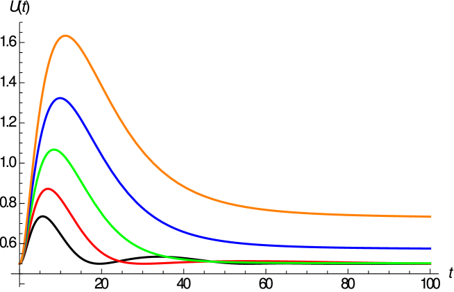
Figure 1: The uncertainty product versus time for a free dissipative dynamics: $\gamma_{I}=-0.1$ (black curve), $\gamma_{I}=-0.05$ (red curve), $\gamma_{I}=0$ (green curve), $\gamma_{I}=0.05$ (blue curve) and $\gamma_{I}=0.1$ (orange curve). For numerical calculations we have used $m=1$, $\hbar=1$, $\sigma_{0}=1$, $q(0)=-20$, $\dot{q}(0)=4$ and $\gamma_{R}=0.1$.

In Figure 1, the uncertainty product is plotted for a free dissipative dynamics ($V=0$ and $F_{r}=0$) and for a given $\gamma_{R}$ but different values of $\gamma_{I}$: $\gamma_{I}=-0.1$ (black curve), $\gamma_{I}=-0.05$ (red curve), $\gamma_{I}=0$ (green curve), $\gamma_{I}=0.05$ (blue curve) and $\gamma_{I}=0.1$ (orange curve). For numerical calculations we have used $m=1$, $\hbar=1$, $\sigma_{0}=1$, $q(0)=-20$, $\dot{q}(0)=4$ and $\gamma_{R}=0.1$. One clearly sees that the uncertainty product increases first and after reaching a maximum value depending on $\gamma_{I}$, it decreases smoothly except for $\gamma_{I}=-0.1$ which another maximum is seen. Note that for the soliton-like solution (61) with $\gamma_{I}=-0.5$, the uncertainty product is independent of time and has the minimum value $0.5$. The asymptotic values observed for each case are greater than 0.5, increasing with the imaginary part of the friction coefficient.

IV.2 Diffusion coefficient for the Brownian-Bohmian motion

In this subsection we are going to take into account the effect of thermal fluctuations in the environment ($F_{r}\neq 0$). The simplest system is the Brownian motion of a particle subject only to a Gaussian white noise. When considering this motion in the Bohmian framework, we talk about the Brownian-Bohmian motion NaMi-book-2017 . For free propagation ($V=0$) solution of the classical Langevin equation (59) is given by MoMi-submitted-2019

$$q(t) = q(0)+\dot{q}(0)\frac{1}{\gamma}(1-e^{-\gamma t})+\frac{1}{m\gamma}\int_{0}^{t}d\tau F_{r}(\tau)e^{-\gamma(t-\tau)}.$$

Then from the properties (62) and (63) of the random force and the Maxwell-Boltzmann distribution for the initial velocities, $f_{T}(\dot{q}(0))=\sqrt{\frac{m}{2\pi k_{B}T}}\exp\left[-\frac{m\dot{q}(0)^{2}}{2k_{B}T}\right]$, one obtains

$$\langle\langle(q(t)-q(0))^{2}\rangle\rangle = 2\frac{k_{B}T}{m\gamma_{R}}\left(t-\frac{1-e^{-\gamma_{R}t}}{\gamma_{R}}\right)$$ (69)

for the mean squared displacement (MSD) where the double averaging implies average over the noise and the initial velocities which are distributed according to the Maxwell-Boltzmann distribution function, $\langle\langle\cdots\rangle\rangle=\int d\dot{q}(0)~{}f_{T}(\dot{q}(0))~{}\langle\cdots\rangle$.

Eq. (69) implies that in the diffusion regime $t\gg\gamma^{-1}_{R}$, MSD is proportional to time with a constant given by $2D$ where $D=k_{B}T/m\gamma_{R}$ is the diffusion constant (Einstein’s law). A time-dependent diffusion coefficient $D(t)$ can be defined as the ratio of MSD over $2t$ MoMi-submitted-2019 . From eqs. (58) and (69), MSD $\langle\langle(x(x^{(0)},t)-x^{(0)})^{2}\rangle\rangle$ of Bohmian stochastic trajectories averaged over initial Bohmian positions $x^{(0)}$ according to the Born distribution rule gives MoMi-submitted-2019

$$D_{\text{q}}(t) = D_{\text{cl}}(t)+\frac{1}{2t}(\sigma(t)-\sigma(0))^{2},\qquad D_{\text{cl}}(t)=\frac{k_{B}T}{m\gamma_{R}}\left(1-\frac{1-e^{-\gamma_{R}t}}{\gamma_{R}t}\right)$$ (70)

for the quantum diffusion coefficient where $D_{\text{cl}}(t)$ is the corresponding classical quantity. For the soliton-like solution (61), quantum diffusion coefficient is exactly the same as that of classical mechanics which leads to the same diffusion constant for both classical and quantum mechanics.

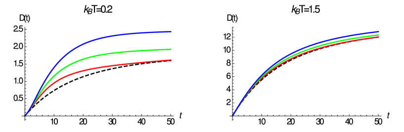
Figure 2: Classical diffusion coefficient (dashed black curves) and quantum diffusion coefficients versus time for $k_{B}T=0.2$ (left panel) and $k_{B}T=1.5$ (right panel) for Brownian-Bohmian motion for $\gamma_{I}=-0.1$ (red curves), $\gamma_{I}=0$ (green curves) and $\gamma_{I}=0.1$ (blue curves). Other parameters are the same as those of Fig. 1.

In Fig. 2, the classical (dashed black curves) and quantum diffusion coefficients (color curves) versus time are plotted for $k_{B}T=0.2$ (left panel) and $k_{B}T=1.5$ (right panel) for the Brownian-Bohmian motion with $\gamma_{I}=-0.1$ (red curves), $\gamma_{I}=0$ (green curves) and $\gamma_{I}=0.1$ (blue curves). Other parameters are the same as those of Fig. 1. It is clearly seen in both panels that eah curve tends to an asymptotic value from which the corresponding diffusion constant can be extracted. As expected from Einstein’s relation, this constant is greater for higher temperatures. Even more, quantum constants are always greater than classical ones due to the width contribution of the wave packet after eq. (70). It should be again emphasized here that $q(t)$ follows a classical Langevin equation with friction $\gamma_{R}$ and $\sigma(t)$ depends on $\gamma_{R}$ and $\gamma_{I}$ at the same time according to the generalized Pinney equation (60).

IV.3 Stochastic transmission through a transient parabolic repeller. Early arrivals

A number of interesting phenomena are seen in time-dependent quantum systems. Among these, one can mention the phenomenon of early arrivals HoMaMa-JPA-2012 ; superarrivals which has been reported in the scattering of wave packets from time-dependent barriers for isolated systems. Before the transmission probability reaches its stationary value, there is a time-interval where an enhancement of this probability with time is seen as compared to the case of free wave packet propagation. Early arrivals refer to this early increase (relative to the free case) in the transmission probability. It is then very illustrative to study this effect for open quantum systems. To this end we consider stochastic transmission from a time-dependent barrier

$$V(x,t) = -\frac{1}{2}m\omega^{2}e^{-g(t-t_{B})^{2}}x^{2}$$ (71)

which corresponds to the appearance of a parabolic repeller during a short time interval by choosing a Gaussian form for the time window, with the parameters $t_{B}$ and $g$ displaying the peak time and inverse width of the window, respectively. Here, $\omega$ characterizes the strength of the barrier. Let us consider a wave packet initially well localized in the left side of the barrier which is sent towards the barrier. The transmission probability is given by

$$P_{\text{tr}}(t) = \int_{x_{d}}^{\infty}dx~{}\rho(x,t)=\frac{1}{2}\mbox{erfc}\left[\frac{x_{d}-q(t)}{\sqrt{2}\sigma(t)}\right]$$ (72)

where $x_{d}$ is the detector location and in the second equality we have used the Gaussian ansatz (18). For the pure dissipative dynamics, we fix $t_{B}$ by $q_{f}(t_{B})=0$ where $f$ denotes the free case i.e., the strength of the barrier is maximum when the center of the free Gaussian packet arrives at the top of the barrier. Thus, from the solution of eq. (59) for the free dissipative dynamics we have

$$t_{B} = -\frac{1}{\gamma_{R}}\ln\left(1+\gamma_{R}\frac{q(0)}{\dot{q}(0)}\right).$$ (73)

Noting the negative sign of $q(0)$ and positive $\dot{q}(0)$ and in order to have a positive time $t_{B}$ we must impose the condition

$$\gamma_{R}\frac{|q(0)|}{\dot{q}(0)} < 1.$$ (74)

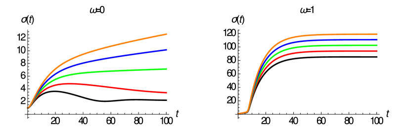
Figure 3: Width of the wave packet versus time for a dissipative dynamics in free motion, $\omega=0$ (left panel), and $\omega=1$ (right panel) for different values of the imaginary part of the friction coefficient: $\gamma_{I}=-0.1$ (black curves), $\gamma_{I}=-0.05$ (red curves), $\gamma_{I}=0$ (green curves), $\gamma_{I}=0.05$ (blue curves) and $\gamma_{I}=0.1$ (orange curves). For numerical calculations we have used $g_{0}=1$ and $x_{d}=20$. Other parameters are the same as those used in Fig. 1.

In Figure 3, the width of the wave packet is plotted versus time for the free dissipative case, $\omega=0$ (left panel), and $\omega=1$ (right panel) for different values of the imaginary part of the friction coefficient: $\gamma_{I}=-0.1$ (black curves), $\gamma_{I}=-0.05$ (red curves), $\gamma_{I}=0$ (green curves), $\gamma_{I}=0.05$ (blue curves) and $\gamma_{I}=0.1$ (orange curves). For numerical calculations, $g_{0}=1$ and $x_{d}=20$ have been chosen. Other parameters are the same as those of Fig. 1. These results show that the width increases globally with the strength of the barrier and with $\gamma_{I}$ and its asymptotic value is rapidly reached for the highest strength case. Furthermore, negative values of $\gamma_{I}$ lead to narrower widths, being the time dependence not so regular. This behavior is in accord to the results of Ref. BBMy-AP-1976 where a logarithmic potential added to the usual linear Schrödinger equation converts it to a non-linear equation and acts against the spreading of the wave packet.

Concerning transmission probability, since $t_{B}$ and $q(t)$ are dependent on $\gamma_{R}$ and not on $\gamma_{I}$ after the behavior of the complementary error function, it is concluded that this probability should increase with the imaginary part of the friction coefficient when its real part remains constant. In Figure 4, the transmission probability (72) versus time is plotted for a non-dissipative dynamics (left panel) and different dissipative dynamics (right panel) for a fixed value of $\gamma_{R}$ but different values of $\gamma_{I}$ and barrier’s strengths. In particular, the following values have been used: $\gamma=0.1(1-i)$ (dotted curves), $\gamma=0.1$ (solid curves) and $\gamma=0.1(1+i)$ (dashed curves) for different values of barrier strengths: $\omega=0$ (black curves), $\omega=0.8$ (red curves) and $\omega=1.5$ (green curves). Other parameters are the same as those used in Fig. 3. In both dynamics, the stationary value of transmission probability decreases with the barrier strength. In the dissipative case and for a given $\omega$, transmission increases with $\gamma_{I}$ keeping $\gamma_{R}$ fixed. Furthermore, there is always a time interval during which the time-dependent transmission probability is higher for the interacting case than for the free case. This is the so-called superarrivals or early arrivals phenomenon which is seen in transmission through transient barriers HoMaMa-JPA-2012 ; superarrivals . A possible application for a key generation and a procedure to speed-up entanglement between two qubits has been proposed elsewhere HoMaMa-JPA-2012 . Early arrival can be quantified by the ratio HoMaMa-JPA-2012 ; superarrivals

$$\eta_{\omega} = \frac{I_{\omega}-I_{f}}{I_{f}}$$ (75)

where

$$I_{\omega} = \int_{t_{d}}^{t_{c}}dt~{}P_{\text{tr},\omega}(t);\qquad I_{f}=\int_{t_{d}}^{t_{c}}dt~{}P_{\text{tr},f}(t)$$ (76)

are respectively the surface below the time-dependent transmission probability in the interacting and free cases during the time interval $\Delta t=t_{c}-t_{d}$ over which superarrival takes place. At time $t_{d}$ the curve of transmission probability for the interacting case deviates from the corresponding curve for the free case while at $t_{c}$ both curves cross. Now, we examine the magnitude of early arrival for the given value $\omega=1.5$ of the barrier strength. From the information contained in Figure 4 and by using equation (75) Table 1 is obtained.

	$~{}~{}t_{d}~{}~{}$	$t_{c}$	$I_{f}$	$I_{1.5}$	$\eta_{{}_{1.5}}$
$\gamma=0$	5.2	8.8912	0.0814939	0.377325	3.6301
$\gamma=0.1(1+i)$	6.8	26.235	2.71907	6.28026	1.30971
$\gamma=0.1$	6.9	27.74212	2.52066	6.37009	1.52715
$\gamma=0.1(1-i)$	7	32.835	2.71218	7.36953	1.71719

Table 1: Early arrival characterization from the ratio defined in eq. 75.

In this Table, we have chosen the deviation time $t_{d}$ in a way that transmission probability at this time is of the order of $10^{-4}$ for the interacting case while it is $\sim 10^{-11}$ for the free propagation. At the cross time $t_{c}$ transmission time for both free and interacting case are the same to four digits decimals. It should be mentioned that the choice zero as the lower limit of integrals in (76) instead of $t_{d}$ has negligible effect on the above results. In any case, we see that the magnitude of early arrival reduces for dissipative dynamics and for such a dynamics early arrival is higher for negative $\gamma_{I}$.

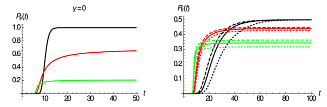
Figure 4: Time-dependent transmission probability for non-dissipative dynamics (left panel) and dissipative dynamics (right panel) with $\gamma=0.1(1-i)$ (dotted curves), $\gamma=0.1$ (solid curves) and $\gamma=0.1(1+i)$ (dashed curves) for different values of barrier’s strength $\omega=0$ (black curves), $\omega=0.8$ (red curves) and $\omega=1.5$ (green curves). Other parameters are the same as those of Fig. 3.

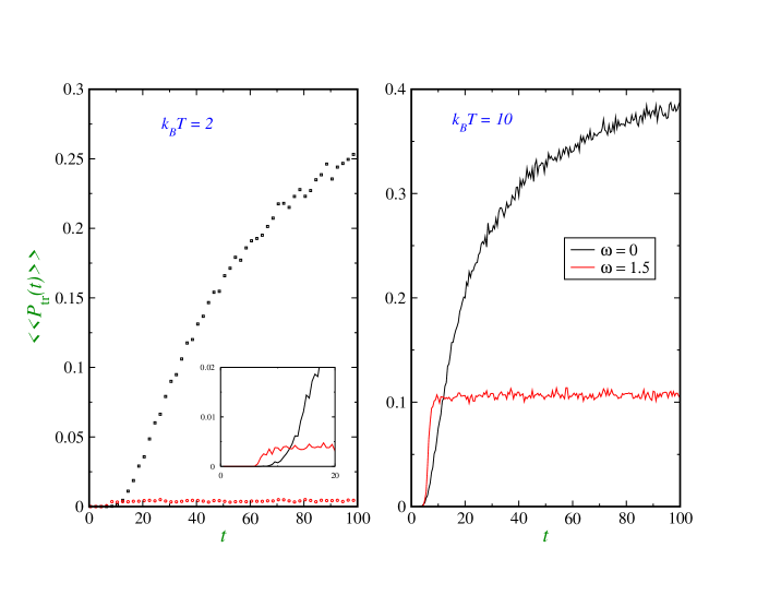
Figure 5: Time-dependent transmission probability in the presence of noise for $k_{B}T=2$ (left panel) and $k_{B}T=10$ (right panel) and for $\gamma_{I}=0$ for different values of barrier’s strength $\omega=0$ (black curves) and $\omega=1.5$ (red curves). Other parameters are the same as those used in Fig. 3. The inset in the left panel clearly displays the early arrival phenomenon.

Finally, in Figure 5, the time-dependent transmission probability under the presence of thermal fluctuations or noise are plotted. The Langevin equation (59) is solved by using an algorithm proposed in VaCi-CPL-2006 with initial conditions $q(t)|_{t=0}=q(0)$ and $\dot{q}(t)|_{t=0}=\dot{q}(0)$ where $\dot{q}(0)$ has a Maxwell-Boltzmann distribution. Then for the thermal transmission probability we have

$$\langle\langle P_{\text{tr}}(t)\rangle\rangle = \sum_{i=1}^{n_{\text{tra}}}P_{\text{tr},i}(t)=\frac{1}{2}\sum_{i=1}^{n_{\text{tra}}}\mbox{erfc}\left[\frac{x_{d}-q_{i}(t)}{\sqrt{2}\sigma(t)}\right]$$ (77)

where in the second equality we have used relation (72) and $q_{i}(t)$ refers to the $i-$th trajectory. For the number of trajectories used to produce a Maxwell-Boltzmann distribution for initial velocities we use $n_{\text{tra}}=10000$. Two different temperatures $k_{B}T=2$ (left panel) and $k_{B}T=10$ (right panel) are used for $\gamma_{R}=0.1$ and $\gamma_{I}=0$. In each panel, two different values of barrier’s strength $\omega=0$ (black curves) and $\omega=1.5$ (red curves) are showed. Here, we have set $t_{B}$ in eq. (71) as $t_{B}=3t_{b}$ where $t_{b}=2m\sigma_{0}^{2}/\hbar$ is the time-scale appearing in the relation of freely propagating Gaussian wave packet in a non-dissipative medium. Again, the phenomenon of early arrivals is seen in this stochastic dynamics. One clearly sees that temperature enhances transmission probability. We observe similar behaviors for non-zero values of $\gamma_{I}$.

V Concluding remarks

Recently, Chavanis has proposed two generalized Schrödinger equations for quantum dissipative systems which although both globally conserve probability density only one fulfills local conservation of the normalization. In both equations, friction coefficient is a complex quantity which the imaginary part (quantum friction) is interpreted as an effective temperature leading to a statisitcal potential when considering an ensemble of particles. Within the Bohmian mechanical framework, both equations have been analyzed in terms of quantum trajectories by considering a Gaussian ansatz for the probability density and simple systems. In the first equation, the center of the wave packet does not follow a classical trajectory revealing that Ehrenfest theorem is violated. We also show contrary to some claims that the SCH equation violates Ehrenfest theorem. The SCH equation is a special case of the NM equation proposed for continuous measurements. For the Gaussian solution, we have also showed by a correct velocity field this equation preserves equivariance property needed for equivalence between results of Bohmian mechanics with those of standard quantum theory.

The second generalized equation is equivalent to the Kostin equation for real frictions while reduces to Bialynicki-Birula and Mycielski equation for imaginary frictions. From this equivalence, we have interpreted the imaginary part of the complex friction coefficient as a factor responsible for soliton-like solutions. In fact, we have observed that for a given negative $\gamma_{I}$, the width of the Gaussian wave packet remains constant in its free propagation. With a Gaussian ansatz for the probability density, Bohmian stochastic trajectories are again obtained.

Acknowledgement

SVM acknowledges support from the University of Qom and SMA support from the Ministerio de Ciencia, Innovación y Universidades (Spain) under the Project FIS2017-83473-C2-1-P.

References

- (1) A. B. Nassar and S. Miret-Artés, Bohmian Mechanics, Open Quantum Systems and Continuous Measurements (Springer, 2017).
- (2) J. M. F. Bassalo, D. G. da Silva, A. B. Nassar and M. S. D. Cattani, J. Adv. Math. Appl. 1 (2012) 1.
- (3) I. Bialynicki-Birula and J. Mycielski, Ann. Phys. 100 (1976) 62.
- (4) H. Bateman, Phys. Rev. 38 (19319) 815.
- (5) P. Caldirola, Nuovo Cimento 18 (1941) 393.
- (6) E. Kanai, Prog. Theor. Phys. 3 (1948) 440.
- (7) L. Diósi and J. J. Halliwell, Phys. Rev. Lett. 81 (1998) 2846.
- (8) M. D. Kostin, J. Chem. Phys. 57 (1972) 3589.
- (9) D. Schuch, K.-M. Chung and H. Hartmann, J. Math. Phys 24 (1983) 1652.
- (10) D. Schuch, Int. J. Quantum Chem. 72 (1999) 537
- (11) D. Süssmann, Seminar Talk at Los Alamos (1973).
- (12) R. W. Hasse, J. Math. Phys. 16 (1975) 2005.
- (13) K. Albrecht, Phys. Lett. B56 (1975) 127.
- (14) M. D. Kostin, J. Stat. Phys. 12 (1975) 146.
- (15) A. B. Nassar, J. Math. Phys. 27 (1986) 2949.
- (16) A. B. Nassar, Int. J. Theor. Phys. 46 (2007) 548.
- (17) A. B. Nassar and S. Miret-Artés, Phys. Rev. Lett. 111 (2013) 150401.
- (18) P.H. Chavanis, Eur. Phys. J. Plus 132 (2017) 286.
- (19) L. Nottale, Scale Relativity and Fractal Space-Time (Imperial College Press, 2011).
- (20) P. Bargueño and S. Miret-Artés, Ann. Phys. 346 (2014) 59.
- (21) A. F. Vargas, N. Morales-Durán and P. Bargueño, Ann. Phys. 356 (2015) 498.
- (22) E. Nelson, Phys. Rev. 150, 1079 (1966).
- (23) R. K. Pathria, Statistical Mechanics, Pergamon Press, Toronto, 1972.
- (24) L. E. Ballentine, Yumin Yang and J. P. Zibin, Phys. Rev. A 50 (1994) 2854.
- (25) P. R. Holland, The Quantum Theory of Motion (Cambridge University Press, 1993).
- (26) D. Dürr, S. Goldstein and N. Zanghi, J. Stat. Phys. 68 (1992) 259.
- (27) D. H Kobe, J. Phys. A: Math. Theor. 40 (2007) 5155.
- (28) S. V. Mousavi and S. Miret-Artés, accepted for publication in EPJ Plus; arXiv:1902.02147
- (29) X. Chen, A. Ruschhaupt, S. Schmidt, A. del Campo, D. Guéry-Odelin and J. G. Muga, Phys. Rev. Lett. 104 (2010) 063002.
- (30) D. Home, A. S. Majumdar and A. Matzkin, J. Phys. A: Math. Theor. 45 (2012) 295301.
- (31) S. Bandyopadhyay, A.S. Majumdar, and D. Home. Phys. Rev. A 65 (2002) 052718; Ali Md Manirul, A. S. Majumdar and D. Home, Phys. Lett. A 304 (2002) 61; H. Karami and S. V. Mousavi, Can. J. Phys. 93 (2015) 413.
- (32) E. Vanden-Eijnden and G. Ciccotti, Chemical Physics Letters 429 (2006) 310–316.