Multi-Component Dark Matter in a Non-Abelian Dark Sector

Abstract

In this paper, we explore a dark sector scenario with a gauged $SU(2)_{{}_{R}}$ and a global $U(1)_{{}_{X}}\times\mathbb{Z}_{2}$, where the continuous symmetries are spontaneously broken to a global $U(1)_{\text{D}}$. We show that in various regions of the parameter space we can have two, or three dark matter candidates, where these dark matter particles are either a Dirac fermion, a dark gauge boson, or a complex scalar. The phenomenological implications of this scenario are vast and interesting. We identify the parameter space that is still viable after taking into account the constraints from various experiments. We, also, discuss how this scenario can explain the recent observation by DAMPE in the electron-positron spectrum. Furthermore, we comment on the neutrino mass generation through non-renormalizable interactions between the standard model and the dark sector.

I Introduction

Despite the numerous successes of the Standard Model (SM) in describing the observed phenomena, there are still intriguing questions that wait to be answered. Arguably, the most important one among them is the nature and origin of dark matter (DM). For some decades, the leading theory was a single component thermal relic with weak size couplings and mass, commonly known as Weakly Interacting Massive Particle. With the advancement of experiments, however, most of the parameter space of a single-component thermal relic has been excluded. Therefore, we are compelled to examine more complex structures of dark sectors. Among the proposed scenarios, multi-component dark matter (MCDM) has attracted a lot of attentions Dienes:2011ja ; Dienes:2011sa ; Bian:2013wna ; Duda:2001ae ; Duda:2002hf ; Profumo:2009tb ; Gao:2010pg ; Feldman:2010wy ; Baer:2011hx ; Aoki:2012ub ; Chialva:2012rq ; Bhattacharya:2013hva ; Esch:2014jpa ; Bian:2014cja ; YaserAyazi:2018lrv ; Ahmed:2017dbb ; DuttaBanik:2016jzv ; DiFranzo:2016uzc ; Dienes:2013xff ; Biswas:2015sva ; Herrero-Garcia:2018qnz ; Karam:2016rsz ; Bhattacharya:2018cgx ; Bhattacharya:2016ysw ; Dev:2016qeb ; Khlopov:1995pa ; Bhattacharya:2017fid ; Huang:2015wts . In these scenarios, the total relic abundance of dark matter is due to the existence of multiple dark matter species. Given the rather complex structure of the SM, it should not be surprising if the dark sector has multiple species as well, but to further motivate MCDM scenarios, the extra degrees of freedom in the dark sector are usually employed to explain some other shortcomings of the SM.

The most common approach in MCDM models is assuming one or multiple symmetries in the dark sector. MCDM models with a gauged $U(1)$ extension or a conserved non-abelian gauge symmetries have already received some attention Ahmed:2017dbb ; DuttaBanik:2016jzv ; Karam:2016rsz ; Bhattacharya:2018cgx ; Bhattacharya:2016ysw ; Davoudiasl:2013jma ; Barman:2018esi ; Gross:2015cwa ; Yamanaka:2015tba ; Dev:2016xcp . In this paper, we focus on a gauged $SU(2)_{{}_{R}}$ times a global $U(1)_{{}_{X}}$ that are spontaneously broken to a global $U(1)_{D}$, once a scalar $\phi$ – a doublet of $SU(2)_{{}_{R}}$ with a non-zero charge under $U(1)_{{}_{X}}$– acquires a vacuum expectation value (vev). Due to this breaking, we have three massive gauge bosons ($W_{{}_{R}}^{\mu}$). We further assume that dark sector respects a $\mathbb{Z}_{2}$ symmetry that stays conserved after the spontaneous symmetry breaking. This $\mathbb{Z}_{2}$ symmetry becomes crucial in making sure we have multiple DM species in various regions of the parameter space. To extend the dynamics of the dark sector, we assume there exists another scalar ($\eta$), and two Dirac Fermions ($\chi_{1}$ and $\chi_{2}$), some of which have the potential to be a dark matter candidate.

The communication of dark sector with the SM content can occur through various means (e.g., kinetic mixing, scalar portal, etc). The kinetic mixing of non-abelian symmetries with any of the SM gauge symmetries is usually non-renormalizable, leading to small interaction between the particles in the two sectors. Therefore, we mainly focus on the scalar portal induced by $\phi$ and the SM Higgs acquiring vevs. This is in many ways similar to a simple Higgs portal model; however, it has some extra advantages that are listed below:

• Large self-interactions between some of the DM candidates: Even though collision-less cold dark matter is successful in describing large scale structures Blumenthal:1984bp , it faces some difficulty describing small scale structures. N-body simulations have shown that Self-Interacting DM can alleviate the small scale structure problems Tulin:2017ara ; Balducci:2018dms . On the other hand, from direct detection experiments, we are led to believe that DM has negligible interactions with nucleons Messina:2018fmz . Therefore, the dark sector could have a non-trivial structure, where it can allow strong self-interaction, while the portal between the dark sector and SM is rather weak. This is easily achieved in our model.

• The extra bosonic degrees of freedom can be used to alleviate the Higgs Hierarchy problem Bian:2013wna ; Chakraborty:2012rb ; Grzadkowski:2009mj ; Karahan:2014ola ; Antipin:2013exa ; Craig:2013xia ; Farina:2013ssa , rescue the vacuum instability Bian:2013wna ; Gonderinger:2009jp ; Drozd:2011aa ; Baek:2012se ; Gabrielli:2013hma ; Hambye:2013sna allow strong first order phase transition, which is needed to prevent baryonic asymmetry from washing out after its generation  Noble:2007kk ; Damgaard:2013kva ; Profumo:2014opa .

• Recently, the DArk Matter Particle Explorer (DAMPE) collaboration released their new measurement of the electron-positron flux in the energy range 25 GeV to 4.6 TeV  Ambrosi:2017wek . The results show a sharp peak above the background around 1.4 $\mathrm{TeV}$. The sharpness of the peak suggests that DM from a nearby source is annihilating to $e^{+}e^{-}$ Yuan:2017ysv ; Fan:2017sor ; Duan:2017pkq ; Gu:2017gle ; Cao:2017ydw ; Liu:2017rgs ; Tang:2017lfb ; Chao:2017yjg ; Gu:2017bdw ; Duan:2017qwj ; Jin:2017qcv ; Niu:2017hqe ; Li:2017tmd ; Gu:2017lir ; Nomura:2017ohi ; Ghorbani:2017cey ; Yang:2017cjm ; Ding:2017jdr ; Liu:2017rgs ; Okada:2017pgr ; Yao:2018ewe ; Beck:2018hau ; Wang:2018pcc ; Balducci:2018dms ; Cao:2017sju ; Cao:2017rjr ; Huang:2015wts . Assuming that the excess is indeed due to the interaction of DM with electrons, to achieve the height of the resonance, the annihilation cross section needs to be much larger than that of the canonical single component thermal relic. To enhance the cross section of dark matter candidates with electrons, we also charge right-handed electron under $SU(2)_{{}_{R}}\times U(1)_{{}_{X}}$. Even though the main motivation for distinguishing right-handed electron is the results of the DAMPE experiment, the annihilation of dark matter candidates to a pair of electron-positron plays a crucial role in setting the relic abundance.

• Neutrino mass generation: Another important observation that cannot be justified within the context of the SM is the mass of neutrinos. In the most minimalistic scenario, we can use the Weinberg operator: $(LH)^{2}/\Lambda$ Weinberg:1979sa , where $\Lambda$ refers to the mass of a heavy Majorana Fermion. A simple calculation reveals that $\Lambda$ has to be bigger than $10^{14}\ \text{GeV}$ Mohapatra:1979ia , which is larger than the Landau pole, and in the regime where we cannot trust the SM framework. With a more complex dark sector, we can connect the mass of neutrinos to some of the degrees of freedom in the dark sector. We still use non-renormalizable operators to get a neutrino mass; however, we find a smaller value for the cut-off scale.

In the following section, we explain the model in greater details and introduce the dark matter candidates. In section III, we find the relic abundance of each DM particles and identify the constraints coming from DM detection experiments. Some comments about neutrino mass generation are given in section III.4. Finally, the concluding remarks are presented in Section IV.

II Model

We study a new physics scenario where the standard model gauge symmetries are augmented by a gauged $SU(2)_{{}_{R}}$ and a global $U(1)_{{}_{X}}\times\mathbb{Z}_{2}$. We supplement the scalar content by two SM singlet scalars: $\phi$ which is a doublet of $SU(2)_{{}_{R}}$:

$$\phi=\begin{pmatrix}\frac{1}{\sqrt{2}}(G_{\phi}^{1}+iG_{\phi}^{2})\\ \\ \varphi^{0}+iG_{\phi}^{3}\end{pmatrix},$$ (1)

with $G^{i}$ being the goldstone bosons, and $\eta$ which is a singlet of $SU(2)_{{}_{R}}$; both $\phi$ and $\eta$ have non-zero charges under $U(1)_{{}_{X}}$. We also extend the Fermionic fields by a doublet $X_{{}_{R}}=(\chi_{2}\leavevmode\nobreak\ \leavevmode\nobreak\ \leavevmode\nobreak\ \chi_{1})^{T}_{{}_{R}}$, and two singlets ($X_{{}_{L}}=\chi_{1}^{L},\chi_{2}^{L})$ of $SU(2)_{{}_{R}}$. These fields are complete singlets of the SM gauge symmetries, but they have a non-zero $U(1)_{{}_{X}}\times\mathbb{Z}_{2}$ charges to avoid mixing with left-handed neutrinos.

Motivated by the DAMPE excess, we also assume right-handed electron is charged under $SU(2)_{{}_{R}}$. For the notation, we use $E_{R}=\left(e^{\prime}\leavevmode\nobreak\ \leavevmode\nobreak\ \leavevmode\nobreak\ e\right)^{T}_{{}_{R}}$, where $e$ is the familiar SM electron, and $e^{\prime}$ is a particle with exactly the same quantum numbers as the right-handed electron. The list of the new particles and their charges is presented in Table 1.

Particles		$SU(2)_{{}_{R}}$		$U(1)_{X}$		$\mathbb{Z}_{2}$		$SU(3)_{C}\times SU(2)_{{}_{L}}\times U(1)_{Y}$
$W_{{}_{R}\mu}$		3		$0$		+		(1     ,   1   ,     0)
$\phi$		2		1/2		+		(1     ,   1   ,     0)
$\eta$		1		2		–		(1     ,   1   ,     0)
$\chi^{1}_{{}_{L}}$		1		1		–		(1     ,   1   ,     0)
$\chi^{2}_{{}_{L}}$		1		2		–		(1     ,   1   ,     0)
$X_{{}_{R}}$		2		3/2		–		(1     ,   1   ,     0)
$E_{{}_{R}}$		2		1/2		+		$\left(1\leavevmode\nobreak\ \leavevmode\nobreak\ \leavevmode\nobreak\ \leavevmode\nobreak\ \leavevmode\nobreak\ ,\leavevmode\nobreak\ \leavevmode\nobreak\ \leavevmode\nobreak\ 1\leavevmode\nobreak\ \leavevmode\nobreak\ \leavevmode\nobreak\ ,\leavevmode\nobreak\ \leavevmode\nobreak\ -1\right)$

Table 1: The quantum numbers of the newly introduced particles under the dark symmetries ($SU(2)_{{}_{R}}\times U(1)_{{}_{X}}\times\mathbb{Z}_{2}$) and the SM symmetries are presented in this table.

In the interaction basis, the Lagrangian of the relevant fields has the following form:

$$\mathcal{L}=\mathcal{L}_{{}_{\text{SM}}}+\mathcal{L}_{{}_{\text{kin}}}+\mathcal{L}_{{}_{\text{Yuk}}}+\mathcal{L}_{{}_{\text{int}}}-V(H,\phi,\eta),$$ (2)

where,

$$\mathcal{L}_{{}_{\text{kin}}} =\frac{1}{4}W^{a}_{{}_{R}\mu\nu}W^{a\mu\nu}_{{}_{R}}+\sum_{i=1,2}\bar{\chi^{i}_{{}_{L}}}(\imath\partial\!\!\!/)\chi^{i}_{{}_{L}}+\bar{X_{{}_{R}}}(\imath D\!\!\!/)X_{{}_{R}}+\bar{E_{{}_{R}}}(\imath D\!\!\!/)E_{{}_{R}}$$

$$+(D_{\mu}\phi)^{\dagger}(D^{\mu}\phi)+(\partial_{\mu}\eta)^{\dagger}(\partial^{\mu}\eta),$$

$$\mathcal{L}_{{}_{\text{Y}}}\ =\tilde{Y}_{1}\bar{X}_{{}_{R}}\phi\chi^{1}_{{}_{L}}+\tilde{Y}_{2}\bar{X}_{{}_{R}}\tilde{\phi}\chi^{2}_{{}_{L}}+\frac{y_{e}}{\Lambda}(\bar{L}H)(\phi^{\dagger}E_{{}_{R}})+h.c.,$$

$$\mathcal{L}_{{}_{\text{int}}} =\frac{y_{\chi_{L}}}{\Lambda^{\prime}}(\bar{L^{c}}\tilde{H}^{\star})(\eta^{\star}\chi^{{}^{L}}_{2})+h.c.$$ (3)

In the kinetic Lagrangian, $D_{\mu}=\partial_{\mu}+ig_{{}_{R}}\frac{\tau^{a}}{2}W_{{}_{R}\mu}^{a}+ig_{{}_{Y}}B_{{}_{\mu}}$, with $g_{{}_{R}}$ being the coupling of the $SU(2)_{{}_{R}}$, and $g_{{}_{Y}}$ is the hypercharge value. The $SU(2)_{{}_{R}}$ field tensor is shown by $W^{\mu\nu}_{{}_{R}}=\partial^{\mu}W_{{{}_{R}}}^{\nu}-\partial^{\nu}W_{{{}_{R}}}^{\mu}-ig_{{}_{R}}[W_{{}_{R}}^{\mu},W_{{}_{R}}^{\nu}]$. In this Lagrangian, $\tilde{Y}_{i}$ are the Yukawa coupling between $\chi_{i}$ and $\phi$, $\tilde{\phi}=\imath\tau^{2}\phi^{\star}$ and $\tilde{H}=\imath\tau^{2}H^{\star}$. The last term in the Yukawa Lagrangian is the electron Yukawa interaction which due to the charge of $E_{{}_{R}}$ under $SU(2)_{{}_{R}}$ becomes non-renormalizable. Another higher dimensional operator that becomes important in figuring out the dynamics of the dark sector is shown in $\mathcal{L}_{{}_{\text{int}}}$. The cut-off scale appearing in $\mathcal{L}_{{}_{\text{int}}}$ does not have to be the same as the one appearing in the electron Yukawa (e.g, $\Lambda\neq\Lambda^{\prime}$), and so we distinguish between them.

To write the scalar potential, $V(H,\phi,\eta)$, we first need to comment on whether the new symmetries stay conserved or are broken. To ensure massive gauge bosons and fermions in the dark sector, we assume $\phi$ acquires a vacuum expectation value (vev) and thus breaks the $SU(2)_{{}_{R}}\times U(1)_{{}_{X}}$ at the scale $v_{\phi}$. Consequently, the scalar potential becomes

$$V(H,\phi,\eta) =-\mu_{{}_{H}}^{2}H^{\dagger}H-\mu_{{}_{\phi}}^{2}\phi^{\dagger}\phi+\mu_{{}_{\eta}}^{2}\eta^{\dagger}\eta$$

$$+\lambda_{{}_{H}}(H^{\dagger}H)^{2}+\lambda_{{}_{\phi}}(\phi^{\dagger}\phi)^{2}+\lambda_{{}_{\eta}}(\eta^{\dagger}\eta)^{2}$$

$$+\xi_{{}_{H\phi}}(H^{\dagger}H)(\phi^{\dagger}\phi)+\xi_{h}(H^{\dagger}H)(\eta^{\dagger}\eta)+\xi_{\phi}(\phi^{\dagger}\phi)(\eta^{\dagger}\eta).$$ (4)

Note that since $\phi$ is even under the $\mathbb{Z}_{2}$ symmetry, the $\mathbb{Z}_{2}$ symmetry stays conserved after the spontaneous symmetry breaking (SSB). Before moving on to the phenomenological effects of the $SU(2)_{{}_{R}}\times U(1)_{{}_{X}}$ and the Electroweak SSB, we note that the stability of the vacuum puts some constraints on the couplings of the scalar potential Kannike:2012pe

$$\lambda_{H},\lambda_{\phi},\lambda_{\eta}>0,\hskip 14.45377pt\xi_{H\phi}>-2\sqrt{\lambda_{H}\lambda_{\phi}},\hskip 14.45377pt\xi_{h}>-2\sqrt{\lambda_{H}\lambda_{\eta}},\hskip 14.45377pt\xi_{\phi}>-2\sqrt{\lambda_{\phi}\lambda_{\eta}},$$

$$\sqrt{\lambda_{H}\lambda_{\phi}\lambda_{\eta}}+\xi_{H\phi}\sqrt{\lambda_{\eta}}+\xi_{h}\sqrt{\lambda_{\phi}}+\xi_{\phi}\sqrt{\lambda_{H}}\geqslant 0,$$

$$\lambda_{H}\lambda_{\phi}\lambda_{\eta}-(\xi_{H\phi}^{2}\lambda_{\eta}+\xi_{h}^{2}\lambda_{\phi}+\xi_{\phi}^{2}\lambda_{H})+2\xi_{H\phi}\xi_{h}\xi_{\phi}\geqslant 0.$$

From minimizing the potential, we can find the values of the vevs:

$$v_{h}^{2}=\frac{4\lambda_{{}_{\phi}}\mu_{{}_{H}}^{2}-2\xi_{{}_{H\phi}}\mu_{{}_{\phi}}^{2}}{4\lambda_{{}_{H}}\lambda_{{}_{\phi}}-\xi_{{}_{H\phi}}^{2}},\hskip 14.45377ptv_{\phi}^{2}=\frac{4\lambda_{{}_{H}}\mu_{{}_{\phi}}^{2}-2\xi_{{}_{H\phi}}\mu_{{}_{H}}^{2}}{4\lambda_{{}_{H}}\lambda_{{}_{\phi}}-\xi_{{}_{H\phi}}^{2}}.$$ (5)

One of the most important consequences of the $SU(2)_{{}_{R}}\times U(1)_{{}_{X}}$ and Electroweak SSB is the inducement of the scalar portal. That is the mixing between the neutral CP-even component of the Higgs field and that of the $\phi$ field. As a result of this mixing, we have two scalars in the mass basis that interact with both the SM sector and dark sector as a function of the mixing angle $\alpha$. That is

$$\begin{pmatrix}h\\ \varphi\end{pmatrix}=\begin{pmatrix}c_{\alpha}&-s_{\alpha}\\ s_{\alpha}&c_{\alpha}\end{pmatrix}\begin{pmatrix}h^{0}\\ \varphi^{0}\end{pmatrix},$$ (6)

where $h^{0}$ and $\varphi^{0}$ are the CP-even component of the Higgs and $\phi$ doublet, respectively, and $h$ and $\varphi$ are the physical fields in the mass basis. We have used $c_{\alpha}=\cos\alpha$ and $s_{\alpha}=\sin\alpha$, with $\alpha$ being

$$\alpha=\frac{1}{2}\tan^{-1}\frac{\xi_{{}_{H\phi}}v_{h}v_{\phi}}{v_{h}^{2}\lambda_{{}_{H}}-v_{\phi}^{2}\lambda_{{}_{\phi}}}.$$

The masses of the scalars are, therefore,

$$m_{h}^{2} =v_{h}^{2}\lambda_{{}_{H}}+v_{\phi}^{2}\lambda_{{}_{\phi}}-(v_{\phi}^{2}\lambda_{{}_{\phi}}-v_{h}^{2}\lambda_{{}_{H}})/\cos(2\alpha),$$

$$m_{\phi}^{2} =v_{h}^{2}\lambda_{{}_{H}}+v_{\phi}^{2}\lambda_{{}_{\phi}}+(v_{\phi}^{2}\lambda_{{}_{\phi}}-v_{h}^{2}\lambda_{{}_{H}})/\cos(2\alpha),$$

$$m_{\eta}^{2} =\mu_{\eta}^{2}+\xi_{h}v_{h}^{2}+\xi_{\phi}v_{\phi}^{2}.$$

Similarly, we can find the masses of the dark gauge bosons and the fermions:

$$m_{{}_{W_{{}_{R}}}}=\frac{g_{{}_{R}}v_{\phi}}{\sqrt{2}},\hskip 21.68121ptm_{\chi_{i}}=\frac{y_{\chi_{i}}v_{\phi}}{\sqrt{2}}.$$ (7)

One important difference between this symmetry breaking and the EW symmetry breaking is that $U(1)_{{}_{X}}$ is global, and thus does not effect the covariant derivative. Hence, the masses of all of the three gauge bosons associated with $SU(2)_{{}_{R}}$ ($W_{{}_{R}}$) are the same.

In this article, we are interested in the phenomenology of the dark matter candidates, and thus it is important to figure out which dark sector particles are cosmologically stable. Given that $SU(2)_{{}_{R}}\times U(1)_{{}_{X}}$ is broken, we need to revisit the conserved symmetries at low scales. Studying the Lagrangian after the SSB, we can convince ourselves that there is a residual $U(1)_{\text{D}}$ symmetry along with the original $\mathbb{Z}_{2}$ symmetry, which leads to the stability of at least two particles in the dark sector. The charges of various particles under the $U(1)_{\text{D}}\times\mathbb{Z}_{2}$ symmetry is shown in Table 2, where the $U(1)_{\text{D}}$ charges are simply $(I_{3})_{{}_{R}}+X$, with $X$ being their charges under $U(1)_{{}_{X}}$.

As $e^{\prime}$ has electromagnetic charge, it is not a good dark matter candidate. Therefore, we must assume $m_{e^{\prime}}\gg m_{W_{{}_{R}}}$. Among the other particles listed in Table 2, $W^{3}_{{}_{R}}$ is also not a DM candidate because it is not charged under either of the $U(1)_{\text{D}}\times\mathbb{Z}_{2}$ symmetries. More specifically, as long as $m_{W_{{}_{R}}}>2m_{e}$ (which as we will show later, the collider constraints require this condition to be true), we can always have the decay of $W^{3}_{{}_{R}}\to e^{+}e^{-}$. The rest of the particles mentioned in Table 2 are connected through the Feynman diagram shown in Fig. 1. Depending on the masses of the dark sector particles, they can decay to each other. For simplicity, we will assume $m_{\chi_{2}}$ is considerably larger than the rest of them, so the true players in the DM phenomenology are $\chi_{1}$, $W^{\pm}_{{}_{R}}$ and $\eta$.

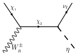
Figure 1: Dark matter candidates $(\chi_{1},W^{\pm}_{{}_{R}},\eta)$ are connected to each other through these diagrams.

		$\hskip 36.135pt\mathbb{Z}_{2}\hskip 36.135pt$			$\hskip 36.135ptU(1)_{\text{D}}\hskip 36.135pt$
$\chi_{2}$		–			2
$\chi_{1}$		–			1
$e^{\prime}$		+			1
$W_{{}_{R}}^{\pm}$		+			$\pm 1$
$W_{{}_{R}}^{3}$		+			0
$\eta$		–			2

Table 2: The charges of the newly introduced particles under the $U(1)_{D}\times\mathbb{Z}_{2}$ symmetries which are the left over symmetries after the SSB. The lightest particle charged under either of the $U(1)_{\text{D}}$ and $\mathbb{Z}_{2}$ symmetries are dark matter candidates.

Collecting the relevant free prameters of our model, we can categorize them into

$$\text{Scales}:v_{\phi},m_{\eta},y_{\chi_{L}}/\Lambda^{\prime},$$

$$\text{Couplings}:g_{{}_{R}},y_{\chi_{i}},\xi_{h},\xi_{\phi},$$

$$\text{Mixing Angles}:\alpha.$$

Particles in the dark sector can interact with SM particles via the scalar portal as well as the direct coupling of the right-handed electrons to dark gauge bosons. In the following section, we first identify the dark matter candidates in each region of the parameter space and then find their relic abundance. We also explain the constraints various experiments impose on the parameter space. However, before diving into the phenomenology, we first address the issue of gauge anomaly that is present in the model.

II.1 Anomaly

The gauged $SU(2)_{{}_{R}}$ symmetry we have introduced is anomalous. Since gauge anomalies are dangerous, we need to extend the model to cancel the anomalies.

• 1) Among the triangle diagrams, $SU(2)_{{}_{R}}^{3}$ is also anomaly free, due to the traceless-ness of the $SU(2)$ symmetries.

• 2) The triangle diagram with $\left[SU(2)_{{}_{R}}\right]^{2}U(1)_{Y}$ would be anomaly-free if and only if the sum of the chiral fermion hypercharges going through the loop is 0 (e.g., $\sum Y=0$).

• 3) Another triangle diagram that leads to gauge anomaly is $\left[Y(1)_{Y}\right]^{3}$, which requires the sum of the cube of hypercharges to vanish (e.g., $\sum Y^{3}=0$).

From the points listed above, it is clear that only $E_{{}_{R}}$ leads to gauge anomalies, because it is charged under both $SU(2)_{{}_{R}}$ and $U(1)_{Y}$. The minimal way to cancel the anomalies mentioned in $(2)$ and $(3)$ is to introduce another a doublet of $SU(2)_{{}_{R}}$ that has hypercharge $+1$, which we call $\Psi=(\psi_{1}\leavevmode\nobreak\ \leavevmode\nobreak\ \leavevmode\nobreak\ \psi_{2})^{T}$ , and $\psi_{3}$ which is a singlet of $SU(2)_{{}_{R}}$ with $Y=-1$.

We will have to assume that the mass of $\psi_{i}$ are large enough that it would not interfere with our phenomenology, but not too large that it would decouple from the theory and leave the model anomalous. To achieve this goal, we will assume there are some vector-like fermions, $f_{i}$, that can mix with $\psi_{i}$s after $\phi$ acquires a vev, and thus give $\psi_{i}$s some mass. Specifically, we will extend our model to include the fermions mentioned in Table 3.

Particles		$SU(2)_{{}_{R}}$		$U(1)_{Y}$		$U(1)_{X}$
$E_{{}_{R}}$		2		-1		1/2
$\Psi$		2		+1		$q_{\Psi}$
$\psi_{3}$		1		-1		$q_{\psi}$
$f_{e^{\prime}}$		1		-1		$1$
$f_{1}$		1		1		$q_{\Psi}+1/2$
$f_{2}$		1		1		$q_{\Psi}-1/2$
$f_{3}$		2		-1		$q_{\psi}+1/2$

Table 3: The quantum numbers of the fermions we need to include in our model to make sure the model is consistent. The $q_{k}$ with $k=\Psi,\psi$ can be any arbitrary numbers, as long as $q_{\psi}\neq 0$. The $f_{i}$, with $i=1,2,3,e^{\prime}$ fermions are vector-like fermions that will mix with the mentioned chiral fermions after $\phi$ gets vev, and lead to a mass for chiral fermions.

The Lagrangian terms that lead to a mass for $\psi_{i}$ and $e^{\prime}$ are:

$$\mathcal{L}_{\text{VL}}\supset y_{e^{\prime}}\bar{E}\tilde{\phi}f_{e^{\prime}}+y_{\psi_{1}}\bar{\Psi}\tilde{\phi}f_{1}+y_{\psi_{2}}\bar{\Psi}\phi f_{2}+y_{\psi_{3}}\bar{f}_{3}\phi\psi_{3}+\sum_{i}M_{f_{i}}\bar{f}_{i}f_{i},$$ (8)

where $i=e^{\prime},1,2,3$ in the last Lagrangian term. We take $M_{f_{i}}$ to be on the order of $v_{\phi}$ so that $e^{\prime},\psi_{i}$ can acquire a mass at or below $v_{\phi}$. However, we will assume that these masses are near $m_{\chi_{2}}$ and thus larger than all of our dark matter candidates. Furthermore, taking $v_{\phi}\sim O(2-10\text{TeV})$, we can also be sure that the existence of these particles does not violate the current search on exotic particles with electromagnetism charge Schael:2013ita . It is also noteworthy to mention that we assume there are no vector-like fermions with quantum numbers $(SU(2)_{{}_{R}},U(1)_{Y},U(1)_{{}_{X}})=(1,-1,0)$ to avoid new contribution to the electron mass.

Having gone over the issue of gauge anomaly, we can now be confident that our theory is consistent. Hence, we can study the phenomenology of DM candidates in the subsequent section.

III Dark Matter Candidates

For having a reliable DM model, the DM particles must be long-lived and produce the correct relic density and satisfy the limits of direct and indirect searches. In this section, we examine each of these steps, starting with identify the stable dark sector particles in various regions of the parameter space.

Stability of the DM candidates:

The simplest way to ensure the stability of DM candidates is using the symmetries of the model. There is a $U(1)_{\text{D}}\times\mathbb{Z}_{2}$ symmetry that stays conserved after the SSB. Therefore, the lightest particles charged under these symmetries are DM candidate. Taking $e^{\prime}$ and $m_{\chi_{2}}$ to be heavier than $\chi_{1}$, $W_{{}_{R}}$ and $\eta$, we have the following DM candidates:

• $m_{W_{{}_{R}}}>m_{\chi_{1}}+m_{\eta}$ : $\eta$ and $\chi_{1}$;

• $m_{\eta}>m_{\chi_{1}}+m_{W_{{}_{R}}}$ : $W_{{}_{R}}$ and $\chi_{1}$;

• $m_{\chi_{1}}>m_{W_{{}_{R}}}+m_{\eta}$ : $\eta$ and $W_{{}_{R}}$;

• $|m_{\chi_{1}}-m_{\eta}|<m_{W_{{}_{R}}}<m_{\chi_{1}}+m_{\eta}$ : $\eta$, $W_{{}_{R}}$, and $\chi_{1}$,

where in the last line we have three DM candidates due to the kinematics. The schematic figures of these conditions are shown in Fig. 2. In the following subsection, we calculate the relic abundance for each of these DM candidates.

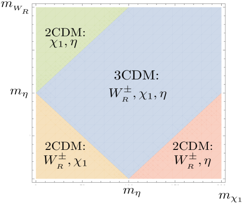
Figure 2: The region of parameter space, where the DM candidates are specified. We have assumed $e^{\prime},\leavevmode\nobreak\ \chi_{2}$ are much heavier than $\chi_{1},W^{\pm}_{{}_{R}},$ and $\eta$ and can decay to lighter dark sector particles.

III.1 Relic Abundance

In thermal Multi-Component Dark Matter (MCDM) scenarios, each dark matter particle starts out in thermal equilibrium with SM particles, and once the temperature falls below the DM mass, DM particles will only annihilate until they freeze-out. The most recent experimental value for relic density $(\Omega_{DM}h^{2}=0.119)$ is reported by Planck collaboration Ade:2015xua . To calculate the DM relic abundance in our model, the coupled Boltzmann equation is applied to study the evolution of the DM particles Springel:2005nw . Assuming thermal relic, we can write:

$$\frac{dn}{dt}+3Hn=-\langle\sigma v\rangle(n^{2}-n^{2}_{eq}),$$ (9)

where $n$ and $n_{eq}$ are denoted the number of density and equilibrium density of the DM particles respectively and $H$ is the Hubbel parameter, and the thermal average annihilation cross section is shown by $\langle\sigma v\rangle$. The annihilation Feynman diagrams for all of the DM components are depicted in Fig 3, where SM denotes $W,Z$ bosons and the top quark.

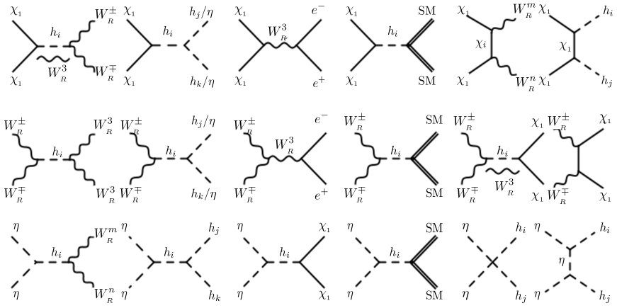
Figure 3: The annihilation Feynman diagrams of DM candidates– Dirac fermion $\chi_{1}$ (first line), dark gauge boson $W_{{}_{R}}$(second line) and complex scalar $\eta$ (third line) are shown. For notation, we have used $h_{i}=h,\varphi$, and SM $=t,W^{\pm},$ and $Z$. For the places where both $\chi_{1}$ and $\chi_{2}$ contribute, we have used $\chi_{i}$, and the places where any of the dark gauge bosons could contribute, we have used $W_{{}_{R}}^{m,n}$.

For Eq. 9 to be valid, we need to make sure $\Gamma_{\chi_{2}}\gg m_{\text{DM}}$. In other words, we want $\chi_{2}$ to decay long before the DM particle become non-relativistic. Therefore,

$$\Gamma_{\chi_{2}}\sim\frac{y_{\chi_{L}}^{2}m_{\chi_{2}}^{3}}{\Lambda^{\prime 2}16\pi^{2}}\gg H=\left.\frac{1.66\sqrt{g_{*}^{\rho}}\ T^{2}}{,}{M_{\text{Pl}}}\right|_{T=m_{\text{DM}}},$$

where $M_{\text{Pl}}$ is the reduced Planck mass and $g_{\star}$ represents the relativistic degrees of freedom at temperature $T$. This constraint puts a mild bound on $\left(\Lambda^{\prime}/y_{\chi_{L}}\right)\lesssim\sqrt{M_{\text{Pl}}\ m_{\chi_{2}}^{3}}/(12\pi m_{\text{DM}})$. For example, if we care about DM particles with $O(\text{TeV})$ mass, and so we take $m_{\chi_{2}}\sim 10\ \text{TeV}$ and $y_{\chi_{L}}\sim O(1)$, we get $\Lambda^{\prime}<5\times 10^{7}\ \text{TeV}$. Furthermore, we need to assume any of the $W^{\pm}_{{}_{R}},\,\chi_{1},$ or $\eta$ that is not DM decay quickly enough that they do not interfere with the relic abundance of DM particles once DM becomes non-relativistic. Hence, if we show the decaying particle by $DM^{\prime}$, we roughly get

$$O(1)\frac{m_{DM^{\prime}}^{5}}{\Lambda^{\prime 2}m_{\chi_{2}}^{2}16\pi^{2}}\gg H=\left.\frac{1.66\sqrt{g_{*}^{\rho}}\ T^{2}}{M_{\text{Pl}}}\right|_{T=m_{\text{DM}}},$$

where $O(1)$ represent the couplings $y_{\chi_{L}}$ and the other couplings involved. Taking $m_{DM^{\prime}}\sim 2\ \text{TeV}$, and using the same benchmarks as before, we arrive at a slightly more stringent bound on $\Lambda^{\prime}<10^{6}\ \text{TeV}$. As long as this condition is satisfied, we can be confident that the decays of heavier dark sector particles do not play a role in the relic abundance of DM candidates.

The only diagram that leads to semi-annihilation between DM candidates is the one shown in Fig. 1, which is roughly

$$\langle\sigma v\rangle_{DM_{1}DM_{2}\to DM_{3}\nu_{\ell}}\sim\frac{g_{{}_{R}}^{2}y_{\chi_{L}}^{2}m_{DM}^{2}}{32\pi\Lambda^{{}^{\prime}2}m_{\chi_{2}}^{2}},$$

where $DM_{i}=\chi_{1},W^{\pm}_{{}_{R}},$ and $\eta$, and we have assumed all of them have roughly the same mass, $m_{DM}$. Using the usual benchmark values: $g_{{}_{R}}\sim y_{\chi_{L}}\sim 1,\ m_{DM}\sim 1\ \text{TeV},m_{\chi_{2}}\sim 10\ \text{TeV},$ and taking $\Lambda^{\prime}\sim 10^{4}\ \text{TeV}$, the semi-annihilation cross section is approximately $10^{-37}\text{cm}^{2}$, and thus is extremely small. Therefore, we ignore the semi-annihilation diagrams. Consequently, the calculation of relic abundance is greatly simplified and the only important ingredient we need is the annihilation cross sections of each of the DM candidates. The analytical expressions of the annihilation diagrams can be found in Appendix A Berlin:2014tja ; Ko:2014gha .

To get a better understanding of the relative sizes of these annihilation process with respect to each other, Fig. 4 shows the cross section of various diagrams where we have fixed: $g_{{}_{R}}=0.65,\ y_{\chi}=\xi_{h}=\xi_{\phi}=0.3$, and $s_{\alpha}=0.1$. We have also fixed $m_{\phi}=v_{\phi}$ and $m_{\chi_{2}}=10\ \text{TeV}$. The left panel of Fig.  4, shows the annihilation $\chi\chi$ to various final states. The red line is $\chi\chi\to e_{{}_{R}}e_{{}_{R}}$ though $W^{3}_{{}_{R}}$, and as we can see it has a very significant rate. $\chi\chi\to\text{SM SM}$, where $SM=t,W^{\pm},Z,h$ is shown in green. The blue line is the cross section of $\chi\chi\to\eta\eta$ times a factor of $10^{10}$, where we have taken $m_{\eta}=3\ \text{TeV}$. This channel opens up for $m_{\chi}>3\ \text{TeV}$ and the rate is very small $(\sim 5\times 10^{-37}\text{cm}^{2})$. With the parameters chosen, $m_{\chi}$ is smaller than $m_{W_{{}_{R}}}$ and $m_{\phi}$ (Eq. 7), and thus the annihilation of $\chi\chi\to W_{{}_{R}}W_{{}_{R}},\phi h,\phi\phi$ does not happen. The middle panel of Fig.  4 shows the annihilation of $W_{{}_{R}}W_{{}_{R}}$ to various final states, where we have again taken $m_{\eta}=3\ \text{TeV}$. The annihilation of $W_{{}_{R}}W_{{}_{R}}\to e_{{}_{R}}e_{{}_{R}}$ is p-wave and thus it is comparatively smaller than $\chi\chi\to e_{{}_{R}}e_{{}_{R}}$. The annihilation of $W_{{}_{R}}$s to SM particles and $\eta$, however, benefit from a higher coupling ($g_{{}_{R}}>y_{\chi}$) and thus it is relatively bigger. Furthermore, the annihilation of $W_{{}_{R}}$ to a pair of $\chi$s is also kinematically possible and has a fairly large rate. Finally, the right panel of Fig.  4 illustrates $\eta$ annihilation, where we have fixed $m_{W_{{}_{R}}}=2\ \text{TeV}$. The resonance at around $2\ \text{TeV}$ is due to $\phi$ becoming on-shell in s-channel annihilations of $\eta$. The yellow line is the annihilation of $\eta\eta\to\phi h$ which opens us for $2m_{\eta}>m_{\phi}+m_{h}$. Other than $\eta\eta\to\text{SM SM }$, the rest of the channels suffer from low rate.

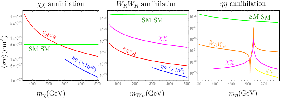
Figure 4: The annihilation of DM candidates to various final states, where we have fixed $g_{{}_{R}}=0.65,\ y_{\chi}=\xi_{h}=\xi_{\phi}=0.3$, $s_{\alpha}=0.1$, $m_{\phi}=v_{\phi}$, and $m_{\chi_{2}}=10\ \text{TeV}$. The left panel is the annihilation of $\chi\chi$, taking $m_{\eta}=3\ \text{TeV}$; the middle panel shows the cross section rates of $W_{{}_{R}}W_{{}_{R}}$ annihilations, where we have again taken $m_{\eta}=3\ \text{TeV}$; and finally the right panel illustrates the annihilation of $\eta\eta$, where $m_{W_{{}_{R}}}$ is fixed to $2\ \text{TeV}$. The red line is the annihilation to a pair of right-handed electrons through s-channel $W^{3}_{{}_{R}}$ mediation. The green line indicates the annihilation to SM particles $=t,W^{\pm},Z,h$. The magenta line is the annihilation of DM candidates to $\chi\chi$, the orange line is the annihilation to a pair of $W_{{}_{R}}$ and the blue line is when the DM particle is annihilating to $\eta\eta$. Because the annihilations to $\eta\eta$ are very small, their cross sections were multiplied by $10^{10}$ (left panel) and $10^{5}$ (middle panel).

Having determined the important processes that set the relic abundance of DM, we move to current constraints on the model parameters. In the following two sub-sections, we study the direct detection, indirect detections as well as the collider constraints. We show that if we insist on using $O(1)$ couplings, the allowed parameter space can be probed with the next generation of experiments.

III.2 Direct Detection

Since, in MCDM, each DM particle shares some portion of the total relic abundance, we expect their annihilation rate to be larger than what would be single component DM $\sim 2.2\times 10^{-26}\text{cm}^{3}/\text{s}$:

$$\Omega_{\text{DM}_{1}}+ \Omega_{\text{DM}_{2}}+\cdots+\Omega_{\text{DM}_{n}}=\Omega_{\text{DM}_{\text{total}}}$$

$$\Rightarrow\Omega_{\text{DM}_{1}}<\Omega_{\text{DM}_{\text{total}}}\Rightarrow\langle\sigma v\rangle_{\text{DM}_{1}}>2.2\times 10^{-26}\text{cm}^{3}/\text{s}$$

Naively, there is a concern that with such large interaction rates of DM with SM particles, it must have been detected at DM experiments, by now. One of the most important constraints on DM models comes from Direct Detection (DD). In our model, DM can scatter with nucleus through Higgs or $\phi$ exchange, leading to potential constraints from DD. Since Higgs portal interactions care about the mass of particles, the interaction of DM with the nucleon is suppressed. In other words, Higgs portal scenarios are efficient in producing the right relic abundance through the annihilation of DM to heavy SM particles, but have a suppressed scattering cross section in DD experiments. This particular reason is common to all Higgs portal DM, and it is one of the benefits of the Higgs portal over generic $Z^{\prime}$ models.

Furthermore, in calculating the relic abundance of $\chi_{1}$ and $W_{{}_{R}}^{\pm}$ DM, their annihilation to a pair of electrons through $W_{{}_{R}}^{3}$ mediator is dominant, especially for large values of $g_{{}_{R}}$. However, this process contributes to DD only at loop level and thus is negligible. This is the second reason that we can have efficient annihilation of $\chi_{1}$ and $W_{{}_{R}}^{\pm}$ DM while being safe from DD bounds.

Since the mediator is a CP-even scalar, the bounds on our model comes from spin-independent DD. Higgs portal DD constraints have been studied in multiple studies, and it is well-known that if DM is a Dirac fermion, $\chi$, then its scattering cross section with the SM is Barger:2007im

$$\sigma_{{\chi_{1}{\text{-N}}}}=\frac{y_{\chi}^{2}\sin^{2}2\alpha}{4\pi}m_{\text{red}}^{2}\left(\frac{1}{m_{h}^{2}}-\frac{1}{m_{\phi}^{2}}\right)^{2}g_{Hp}^{2},$$ (10)

where $g_{{}_{\text{DM}}}$ is the coupling of the DM particle with the scalar mediator, $m_{\text{red}}=m_{p}m_{\text{DM}}/(m_{p}+m_{\text{DM}}),$ and $g_{Hp}$ is the effective coupling of Higgs with proton Djouadi:2012zc :

$$g_{Hp}=\frac{m_{p}}{v_{h}}\left[\sum_{q=u,d,s}f_{q}^{(p)}+\frac{2}{9}\left(1-\sum_{q=u,d,s}f_{q}^{(p)}\right)\right]\approx 1.3\times 10^{-3}.$$ (11)

In the case the dark matter is a gauge boson, its scattering cross section with nucleons goes as the following Baek:2012se :

$$\sigma_{{}_{W_{{}_{R}}\text{-N}}}=\frac{g_{R}^{2}\sin^{2}2\alpha}{4\pi}m_{\text{red}}^{2}\left(\frac{1}{m_{h}^{2}}-\frac{1}{m_{\phi}^{2}}\right)^{2}g_{Hp}^{2},$$ (12)

and finally for a stable scalar it is Casas:2017jjg

$$\sigma_{{}_{\eta{\text{-N}}}}=\frac{m_{p}^{2}}{8\pi m_{\eta}^{2}}m_{\text{red}}^{2}\left(\frac{\xi_{h}c_{\alpha}}{m_{h}^{2}}+\frac{\xi_{\phi}s_{\alpha}}{m_{\phi}^{2}}\right)^{2}g_{Hp}^{2}.$$ (13)

To recast the DD bounds on our model, it is important to realize that each component of DM constitute only a percentage of DM. Assuming their ratio in early universe is the same as the one in the vicinity of earth, we get

$$\sigma_{{}_{\text{DM}\text{-N}}}=\sigma_{{\chi_{1}{\text{-N}}}}\times\frac{\Omega_{\chi_{1}}}{\Omega_{\text{DM}}}+\sigma_{{}_{W_{{}_{R}}\text{-N}}}\times\frac{\Omega_{W_{{}_{R}}}}{\Omega_{\text{DM}}}+\sigma_{{}_{\eta{\text{-N}}}}\times\frac{\Omega_{\eta}}{\Omega_{\text{DM}}}.$$ (14)

In Fig. 5, the DD constraints as well as some other constraints are shown. The purple region is excluded from the DD experiments Messina:2018fmz . The LEP experiment puts a stringent constraint on any particle that interacts with electrons Schael:2013ita . Since right-handed electrons are charged under $SU(2)_{{}_{R}}$, the dark gauge bosons can directly interact with them. The strongest constraint of LEP comes from the Drell-Yan Production of a pair of electrons through an exchange of $W_{{}_{R}}^{3}$, which excludes $m_{W_{{}_{R}}}<2\ \text{TeV}$. This is shown in orange in Fig. 5. The red shaded region is when the indicated particle is no longer a DM candidate because it is not stable. The green region is when $g_{{}_{R}}>1$, which threatens perturbativity. Finally, the gray region is when the relic abundance of all DM candidates combined is too large and they over-close the universe. The green and red dotted lines indicate that the DM introduced in this paper are respectively $50\%$ and $30\%$ of the total DM. The star in the left plot of Fig. 5 is a benchmark, where $55\%$ of the DM is due to the relic abundance of $\chi$ and $45\%$ is from $\eta$. Similarly, the star in the right plot of Fig. 5, indicates a sample point, where $\chi$, $\eta$ and $W_{{}_{R}}$ are respectively $52\%$, $38\%$ and $10\%$ of the total DM. Due to the large cross-section of $W_{{}_{R}}$ to electrons and $\phi$, its relic abundance is usually low.

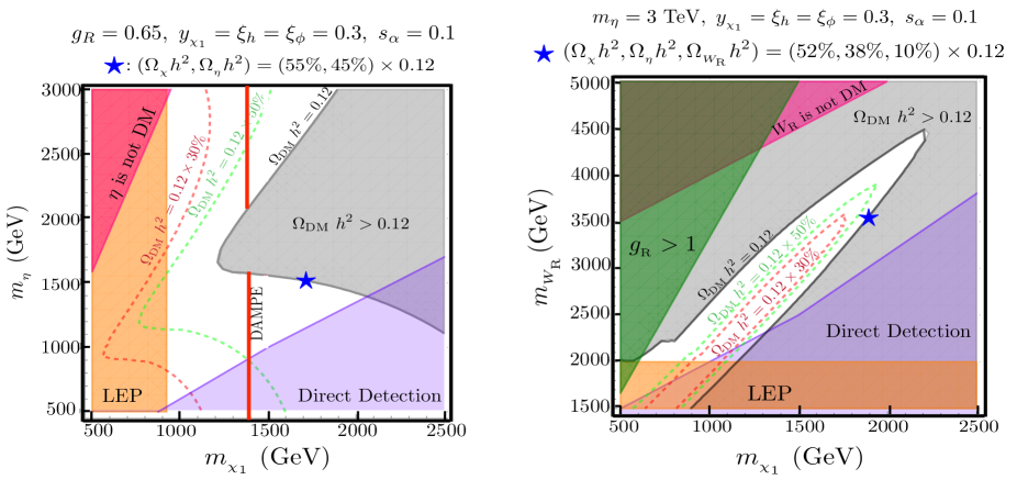
Figure 5: The allowed parameter space for various benchmarks. The solid black dashed green and dashed red shown the contour for producing all, $50\%$, and $30\%$ of the relic abundance of DM, respectively. The shaded gray region is when we over-produce DM. The shaded purple is excluded from DD experiment Messina:2018fmz , and the shaded orange part is excluded by LEP Schael:2013ita . The pink region is when the indicated particle is no longer DM and decays. The green region is when $g_{{}_{R}}>1$ which violates perturbativity. The star is chosen as an example to show how much of DM each particle constitutes. Finally, the solid red line is the region we can explain the DAMPE excess Ambrosi:2017wek .

III.3 Indirect Detection

Another way to constrain our parameter space is by using indirect detection (ID) results. The main annihilation channels of our DM candidates are the production of a pair of electrons or heavy particles. Heavy particles eventually decay to stable particles, which some of them can be detected here on earth. Furthermore, any particle in this process that is electromagnetically charged will radiate photon which can also be detected through various experiments (e.g, Fermi-LAT Ackermann:2013yva ). However, due to the large uncertainty of the background, ID bounds are usually mild. Even considering the strongest bounds of Fermi-LAT, which is $100\%$ branching ratio to $b\bar{b}$, ID can constrain DM only up to a few hundreds of GeV, which is smaller than the benchmarks we are considering.

Recently, the DArk Matter Particle Explorer (DAMPE) experiment Ambrosi:2017wek , which is a satellite-borne, high energy particles and gamma-ray detector, published their measurement of the electron plus positron spectrum. Their result indicates a tentative narrow peak around $\sim 1.4\ \mathrm{TeV}$. The local significance of this excess is about $3.7\sigma$ assuming a broken power-law background Fowlie:2017fya ; Huang:2017egk , and its global significance has been measured to about $2.3\sigma$ Huang:2017egk ; Niu:2017lts ; Ge:2017tkd ; Chao:2017emq ; Nomura:2018jkd ; Yao:2018ewe . Such a narrow peak could be a result of a DM with mass $1.4\ \mathrm{TeV}$ to a pair of right-handed electrons. The interaction of DM with left-handed electrons should be suppressed, due to the results published by IceCube, which reported no excess in the neutrino experiment Zhao:2017nrt . This is the reason we considered only the right-handed electrons being charged under the $SU(2)_{{}_{R}}$.

According to the DAMPE experiment, the annihilation rate to electron-positron is estimated to be much more than the annihilation rate for a single component DM, which further motivates our set up for multi-component DM. However, it is important to make sure the annihilation to electron pair is s-wave.

Among the DM candidates in our set-up, $W_{{}_{R}}^{\pm}$ and $\chi_{1}$ interact with right-handed electrons strongly. The annihilation of $W_{{}_{R}}^{\pm}$ to $e^{+}e^{-}$, however, is p-wave:

$$\langle\sigma v\rangle_{{}_{W_{{}_{R}}W_{{}_{R}}\to e^{+}e^{-}}}=\frac{5\ g_{{}_{R}}^{4}}{216\pi m_{W_{{}_{R}}}^{2}}v^{2}.$$ (15)

Even though this process could play a significant role in setting the abundance of $W_{{}_{R}}^{\pm}$ in the early universe, its rate right now should be negligible. That is because the ambient velocity of DM is estimated to be $v_{\text{DM}}\sim 0.001$. The annihilation of $\chi_{1}\chi_{1}\to e^{+}e^{-}$, on the other hand, is s-wave and thus can have a significant contribution to ID at the current time:

$$\langle\sigma v\rangle_{{}_{\chi_{1}\chi_{1}\to e^{+}e^{-}}}=\frac{8\ g_{{}_{R}}^{4}m_{\chi_{1}}^{2}}{64\pi(m_{W_{{}_{R}}}^{2}-4m_{\chi_{1}}^{2})^{2}}.$$ (16)

Therefore, in the region where $\chi_{1}$ is a DM particle, its annihilation to a pair of electrons could justify the observation of the narrow peak in the DAMPE experiment. The red line in the left panel of Fig. 5, shows the benchmark that could explain the DAMPE observation. It is worth mentioning that even though the main motivation behind charging the right-handed electrons under $SU(2)_{{}_{R}}$ was explaining the DAMPE observation, the annihilation of DM particles to a pair of electrons contributes significantly in setting the relic abundance of DM candidates. In the scenario where right-handed electrons did not interact directly with the dark sector, DM particles had to be about a factor of 5 lighter to not over-close the universe. However, that region of the parameter space is strongly constrained by DD experiments.

III.4 Neutrino Mass

An added bonus of non-minimal structure in the dark sector is that we can attack some other problem of the SM. In this part, we comment on how the neutrino mass can be radiatively generated using the particles in the dar sector. To do so, we will employ the following terms:

$$\frac{y_{\chi_{L}}}{\Lambda^{\prime}}(\bar{L}^{c}\tilde{H}^{\star})(\eta^{\star}\chi_{2}^{L})+\frac{y_{\chi_{{}_{R}}}}{\Lambda^{{}^{\prime}2}}(\eta\bar{X}_{{}_{R}}\tilde{\phi})(\tilde{H}^{\dagger}L)+\tilde{Y}_{2}\bar{X}_{{}_{R}}\tilde{\phi}\chi_{2}^{L}$$ (17)

We can think of $\Lambda^{\prime}$s to be vector-like fermions, one with charge $(SU(2)_{L},U(1)_{Y},U(1)_{X},\mathbb{Z}_{2})$ $=(2,-1/2,2,-)$ and another with charge $(SU(2)_{L},U(1)_{Y},U(1)_{X},\mathbb{Z}_{2})=(1,0,2,-)$. To avoid the contribution of Weinberg operator in giving neutrinos a mass, we will assume there are no Majorana or triplet of $SU(2)_{W}$ in the UV theory. The diagram leading to neutrino mass is shown in Fig. 6.

Given that neutrino mass is expected to be smaller than a few 0.1 eV Giusarma:2016phn ; Giusarma:2018jei we can roughly estimate the value of $\Lambda^{\prime}$ assuming $y_{\chi_{L}}$ and $y_{\chi_{R}}$ are $O(1)$:

$$\frac{v_{h}^{2}v_{\phi}^{2}m_{\chi_{2}}^{2}}{\Lambda^{{}^{\prime}3}m_{\eta}^{2}16\pi^{2}}\lesssim 0.1\ \text{eV}.$$ (18)

Assuming a benchmark value of $v_{\phi}\sim 10\ \text{TeV}$, $m_{\chi_{2}}\sim 10\ \text{TeV}$, and $\eta\sim 3\ \text{TeV}$ we get $\Lambda^{\prime}>2\times 10^{4}\ \text{TeV}$. This constraint combined with the bound we need to satisfy to make sure the decaying particles decay before DM candidates become non-relativisitc requires $\Lambda^{\prime}$ to be roughly in the range of $10^{4}-10^{6}$ TeV.

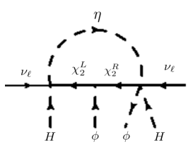
Figure 6: The radiative generation of mass of neutrino through non-renormalizable operators.

IV Conclusions

In this work, we studied a scenario of the dark sector that contains two or three dark matter (DM) candidates. We proposed extending the SM symmetries by a gauge $SU(2)_{{}_{R}}$ and a global $U(1)_{{}_{X}}\times\mathbb{Z}_{2}$, which the continuous symmetries are spontaneously broken to a global $U(1)_{D}$. We considered a case where dark sector contained some Dirac fermions and complex scalars to investigate a dynamic dark sector. To see how our proposed scenario could explain the recent observation by DArk Matter Particle Explorer (DAMPE), we also charged right-handed electrons under $SU(2)_{{}_{R}}$. We assumed $O(1)$ couplings, to consider a more natural scenario. Other than the Higgs portal, which connects the dark sector to the SM, the annihilation of $W_{{}_{R}}$ and $\chi_{1}$ to a pair of electrons happen to play a significant role in the relic abundance of DM particles.

The phenomenology of DM candidates was studied, and the region of the parameter space where they can produce the right relic abundance while being safe from various DM detection experiment was identified. We noticed that only a small region of parameter space survives the constraint and this region could be probed with the next generations of experiments. Additionally, we commented on how neutrinos can gain a mass through non-renormalizable interactions with the dark sector. An important advantage of our scenario over Weinberg operator is that our cut-off scale is $O(10^{4}\ \text{TeV})$, and much lower than the cut-off scale suggested by the Weinberg operator.

In conclusion, we emphasize that in the era where single DM thermal relics are highly constrained, it is important to consider multi-species DM. In the most simplistic paradigm, where DM particles are thermal relics, multi-component DM suggests strong couplings between DM particles and SM. As a result, Leptophilic DM or when there is a Higgs portal models are preferred.

Appendix A The cross section of DM candidates

In this appendix, we show the analytical expressions that we have calculated using FeynCalc Shtabovenko:2016sxi . The first subsection is the potential annihilation cross sections of $\chi$, the second one belongs to $W_{{}_{R}}$ and the last one shows the annihilation cross sections of $\eta$. These processes set the relic abundance of DM if they are 1) kinematically allowed, 2) the indicated initial state is indeed a DM candidate.

A.1 $\chi$ DM

$$\langle\sigma v\rangle_{\chi\chi\to e_{{}_{R}}e_{{}_{R}}}=\frac{8g_{{}_{R}}^{4}m_{\chi}^{2}}{64\pi(4m_{\chi}^{2}-m_{W_{{}_{R}}}^{2})^{2}}$$

$$\langle\sigma v\rangle_{\chi\chi\to t\bar{t}}=\frac{9y_{t}^{2}y_{\chi}^{2}}{8\pi}c_{\alpha}^{2}s_{\alpha}^{2}\frac{(m_{h}^{2}m_{\phi}^{2})^{2}(m_{\chi}^{2}-m_{t}^{2})\sqrt{4m_{\chi}^{2}-m_{t}^{2}}}{m_{\chi}(m_{h}^{2}-4m_{\chi}^{2})^{2}(m_{\phi}^{2}-4m_{\chi}^{2})^{2}}v^{2}$$

$$\langle\sigma v\rangle_{\chi\chi\to WW}=\frac{y_{\chi}^{2}c_{\alpha}^{2}s_{\alpha}^{2}}{8\pi}\frac{(m_{h}^{2}-m_{\phi}^{2})^{2}(3m_{w}^{4}+4m_{\chi}^{4}-4m_{\chi}^{2}m_{w}^{2})\sqrt{4m_{\chi}^{2}-m_{w}^{2}}}{v_{h}^{2}m_{\chi}(m_{h}^{2}-4m_{\chi}^{2})^{2}(m_{\phi}^{2}-4m_{\chi}^{2})^{2}}$$

$$\langle\sigma v\rangle_{\chi\chi\to ZZ}=\frac{y_{\chi}^{2}c_{\alpha}^{2}s_{\alpha}^{2}}{2\pi}\frac{(m_{h}^{2}-m_{\phi}^{2})^{2}(3m_{z}^{4}+4m_{\chi}^{4}-4m_{\chi}^{2}m_{z}^{2})\sqrt{4m_{\chi}^{2}-m_{z}^{2}}}{v_{h}^{2}m_{\chi}(m_{h}^{2}-4m_{\chi}^{2})^{2}(m_{\phi}^{2}-4m_{\chi}^{2})^{2}}$$

$$\langle\sigma v\rangle_{\chi\chi\to hh}=\frac{y_{\chi}^{2}s_{\alpha}^{2}}{64\pi m_{\chi}^{3}v_{h}^{2}(4m_{\chi}^{2}-m_{h}^{2})^{3/2}(4m_{\chi}^{2}-m_{\phi}^{2})}$$

$$\hskip 72.26999pt\left[(18c_{\alpha}^{2}m_{h}^{4}m_{\chi}^{2}(m_{h}^{2}-m_{\phi}^{2})^{2}\right.$$

$$\hskip 72.26999pt+24y_{\chi}v_{h}s_{\alpha}c_{\alpha}m_{h}^{2}sm_{h}^{2}m_{\chi}(4m_{\chi}^{2}-m_{h}^{2})(m_{\phi}^{2}-m_{h}^{2})(4m_{\chi}^{2}-m_{\phi}^{2})$$

$$\hskip 72.26999pt+\left.4y_{\chi}^{2}s_{\alpha}^{2}v_{h}^{2}(4m_{\chi}^{2}-m_{h}^{2})(4m_{\chi}^{2}-m_{\phi}^{2})\right]$$

$$\langle\sigma v\rangle_{\chi\chi\to\phi\phi}=\frac{y_{\chi}^{2}c_{\alpha}^{2}}{32\pi m_{\chi}v_{\phi}^{2}(4m_{\chi}^{2}-m_{h}^{2})^{2}(2m_{\chi}^{2}-m_{\phi}^{2})(4m_{\chi}^{2}-m_{\phi}^{2})^{3/2}}$$

$$\hskip 72.26999pt\left[128\,y_{\chi}^{2}m_{\chi}^{6}v_{\phi}^{2}-12m_{\chi}m_{\phi}^{6}(3m_{\chi}+v_{\phi}y_{\chi})\right.$$

$$\hskip 72.26999pt+4m_{\chi}^{2}m_{\phi}^{4}(9m_{\chi}^{2}+18m_{\chi}v_{\phi}y_{\chi}+2v_{\phi}^{2}y_{\chi}^{2})$$

$$\hskip 72.26999pt-32y_{\chi}m_{\chi}^{4}m_{\phi}^{2}v_{\phi}(3m_{\chi}+2v_{\phi}y_{\chi})$$

$$\hskip 72.26999pt-6c_{\alpha}^{2}s_{\alpha}^{2}m_{\phi}^{2}(4m_{\chi}^{2}-m_{h}^{2})(8m_{\chi}^{4}+m_{\phi}^{4}-6m_{\chi}^{2}m_{\phi}^{2})(8m_{\chi}^{3}v_{\phi}y_{\chi}+3m_{\phi}^{4}-2m_{\chi}m_{\phi}^{2}(3m_{\chi}+v_{\phi}y_{\chi}))$$

$$\hskip 72.26999pt+\left.9s_{\alpha}^{4}m_{\phi}^{4}(8m_{\chi}^{4}+m_{\phi}^{4}-6m_{\chi}^{2}m_{\phi}^{2})^{2}\right]$$

$$\langle\sigma v\rangle_{\chi\chi\to h\phi}=\frac{s_{\alpha}^{2}y_{\chi}^{2}\sqrt{m_{h}^{4}+(4m_{\chi}^{2}-m_{\phi}^{2})^{2}-2m_{h}^{2}(m_{\phi}^{2}-2m_{\chi}^{2})}}{512\pi v_{h}^{2}m_{\chi}^{4}(4m_{\chi}^{2}-m_{h}^{2})^{2}}(4m_{\chi}^{2}-m_{\phi}^{2})^{2}(4m_{\chi}^{2}-m_{\phi}^{2}-m_{h}^{2})^{2}$$

$$\hskip 72.26999pt\left[18s_{\alpha}^{2}m_{h}^{4}m_{\chi}^{2}(4m_{\chi}^{2}-m_{\phi}^{2})^{2}(4m_{\chi}^{2}-m_{\phi}^{2}-m_{h}^{2})^{2}+(m_{h}^{2}(25m_{\phi}^{4}-128m_{\phi}^{2}m_{\chi}^{2}+256m_{\chi}^{4})\right.$$

$$\hskip 72.26999pt-6s_{\alpha}c_{\alpha}y_{\chi}v_{h}^{2}m_{h}^{2}m_{\chi}(4m_{\chi}^{2}-m_{h}^{2})(4m_{\chi}^{2}-m_{\phi}^{2})(4m_{\chi}^{2}-m_{\phi}^{2}-m_{h}^{2})(3\sqrt{2}m_{h}^{2}m_{\phi}^{2}-(4m_{\chi}^{2}-m_{\phi}^{2})(3\sqrt{2}m_{\phi}^{2}+16m_{\chi}^{2}))$$

$$\hskip 72.26999pt+c_{\alpha}^{2}(4m_{\chi}^{2}-m_{h}^{2})^{2}(2m_{h}^{2}m_{\phi}^{2}(4m_{\chi}^{2}-m_{\phi}^{2})(7m_{\phi}^{2}-8(8+3\sqrt{2})m_{\chi}^{2})$$

$$\hskip 72.26999pt\left.+y_{\chi}^{2}v_{h}^{2}(4m_{\chi}^{2}-m_{\phi}^{2})^{2}(25m_{\phi}^{4}+16(3\sqrt{2}-8)m_{\phi}^{2}m_{\chi}^{2}+384m_{\chi}^{4})\right]$$

$$\langle\sigma v\rangle_{\chi\chi\to W_{{}_{R}}W_{{}_{R}}}=\frac{\sqrt{4m_{\chi}^{2}-m_{W_{{}_{R}}}^{2}}}{256\pi m_{\chi}}\left\{\frac{160y_{\chi}^{2}(4m_{\chi}^{2}+3m_{W_{{}_{R}}}^{4}4m_{\chi}^{2}m_{W_{{}_{R}}}^{2})(c_{\alpha}^{2}(4m_{\chi}^{2}-m_{h}^{2})+s_{\alpha}^{2}(4m_{\chi}^{2}-m_{\phi}^{2}))^{2}}{v_{\phi}^{2}(4m_{\chi}^{2}-m_{h}^{2})^{2}(m_{\chi}^{2}-m_{\phi}^{2})^{2}}\right.$$

$$\hskip 72.26999pt-\frac{g_{p}^{4}}{m_{W_{{}_{R}}}^{4}(4m_{\chi}^{2}-m_{W_{{}_{R}}}^{2})^{2}(2m_{\chi}^{2}-m_{W_{{}_{R}}}^{2})^{2}(m_{\chi}^{2}+m_{\chi_{2}}^{2}-m_{W_{{}_{R}}})^{2}}$$

$$\hskip 72.26999pt\left[-128m_{\chi}^{10}((7+2\sqrt{2})m_{\chi}^{4}+2(3+\sqrt{2})m_{\chi}^{2}m_{\chi_{2}}^{2}+3m_{\chi_{2}}^{4})\right.$$

$$\hskip 72.26999pt+(17+12\sqrt{2})m_{W_{{}_{R}}}^{14}-2m_{W_{{}_{R}}}^{12}(5(4\sqrt{2}-9)m_{\chi}^{2}+2(8+3\sqrt{2})m_{\chi_{2}}^{2})$$

$$\hskip 72.26999pt-4m_{W_{{}_{R}}}^{10}(5(60+17\sqrt{2})m_{\chi}^{4}+(50-7\sqrt{2})m_{\chi}^{2}m_{\chi_{2}}^{2}-4m_{\chi_{2}}^{4})$$

$$\hskip 72.26999pt+4m_{W_{{}_{R}}}^{8}((997+508\sqrt{2})m_{\chi}^{6}+2(229+46\sqrt{2})m_{\chi}^{4}m_{\chi_{2}}^{2}-4m_{\chi_{2}}^{4})$$

$$\hskip 72.26999pt+16m_{W_{{}_{R}}}^{6}((379+244\sqrt{2})m_{\chi}^{8}+2(125+52\sqrt{2})m_{\chi}^{6}m_{\chi_{2}}^{2}+50m_{\chi}^{4}m_{\chi_{2}}^{4})$$

$$\hskip 72.26999pt+16m_{\chi}^{6}m_{W_{{}_{R}}}^{4}((249+184\sqrt{2})m_{\chi}^{4}+14(13+10\sqrt{2})m_{\chi}^{2}m_{\chi_{2}}^{2}+75m_{\chi_{2}}^{4})$$

$$\hskip 72.26999pt\left.\left.-64m_{\chi}^{8}m_{W_{{}_{R}}}^{2}(7\sqrt{2}m_{\chi}^{4}+(11\sqrt{2}-4)m_{\chi}^{2}m_{\chi_{2}}^{2}+4m_{\chi_{2}}^{4})\right]\right\}$$

$$\langle\sigma v\rangle_{\chi\chi\to\eta\eta}=\frac{y_{\chi}^{2}\sqrt{4m_{\chi}^{2}-m_{\eta}^{2}}}{8\pi m_{\chi}(4m_{\chi}^{2}-m_{h}^{2})^{2}(4m_{\chi}^{2}-m_{\phi}^{2})^{2}}(c_{\alpha}\xi_{\phi\eta}m_{h}^{2}+4m_{\chi}^{2}(\xi_{h\eta}s_{\alpha}-\xi_{\phi\eta}c_{\alpha})-\xi_{h}s_{\alpha}m_{\phi}^{2})^{2}$$

A.2 $W^{\pm}_{{}_{R}}$ DM

$$\langle\sigma v\rangle_{W_{R}W_{R}\to e_{{}_{R}}e_{{}_{R}}}=\frac{5g_{p}^{4}v^{2}}{216\pi m_{W_{R}}^{2}}$$

$$\langle\sigma v\rangle_{W_{R}W_{R}\to t\bar{t}}=\frac{3m_{W_{R}}c_{\alpha}^{2}s_{\alpha}^{2}y_{t}^{2}\left(m_{h}^{2}-m_{\phi}^{2}\right)^{2}\left(4m_{W_{R}}^{2}-2m_{t}^{2}\right)\sqrt{4m_{W_{R}}^{2}-m_{t}^{2}}}{4\pi v_{\phi}^{2}\left(m_{h}^{2}-4m_{W_{R}}^{2}\right)^{2}\left(m_{\phi}^{2}-4m_{W_{R}}^{2}\right)^{2}}$$

$$\langle\sigma v\rangle_{W_{R}W_{R}\to ZZ}=\frac{2m_{W_{R}}c_{\alpha}^{2}s_{\alpha}^{2}\left(m_{h}^{2}-m_{\phi}^{2}\right)^{2}\sqrt{4m_{W_{R}}^{2}-m_{Z}^{2}}\left(4m_{W_{R}}^{4}-4m_{W_{R}}^{2}m_{Z}^{2}+3m_{Z}^{4}\right)}{3\pi v_{h}^{2}v_{\phi}^{2}\left(m_{h}^{2}-4m_{W_{R}}^{2}\right)^{2}\left(m_{\phi}^{2}-4m_{W_{R}}^{2}\right)^{2}}$$

$$\langle\sigma v\rangle_{W_{R}W_{R}\to WW}=\frac{m_{W_{R}}c_{\alpha}^{2}s_{\alpha}^{2}\left(m_{h}^{2}-m_{\phi}^{2}\right)^{2}\sqrt{4m_{W_{R}}^{2}-m_{W}^{2}}\left(4m_{W_{R}}^{4}-4m_{W_{R}}^{2}m_{W}^{2}+3m_{W}^{4}\right)}{6\pi v_{h}^{2}v_{\phi}^{2}\left(m_{h}^{2}-4m_{W_{R}}^{2}\right)^{2}\left(m_{\phi}^{2}-4m_{W_{R}}^{2}\right)^{2}}$$

$$\langle\sigma v\rangle_{W_{R}W_{R}\to hh}=\frac{3m_{W_{R}}m_{h}^{4}c_{\alpha}^{2}s_{\alpha}^{2}\left(m_{h}^{2}-m_{\phi}^{2}\right)^{2}}{8\pi v_{h}^{2}v_{\phi}^{2}\left(4m_{W_{R}}^{2}-m_{h}^{2}\right)^{3/2}\left(m_{\phi}^{2}-4m_{W_{R}}^{2}\right)^{2}}$$

$$\langle\sigma v\rangle_{W_{R}W_{R}\to\phi\phi}=\frac{3m_{W_{R}}m_{\phi}^{4}\left(c_{\alpha}^{2}\left(m_{h}^{2}-4m_{W_{R}}^{2}\right)+s_{\alpha}^{2}\left(m_{\phi}^{2}-4m_{W_{R}}^{2}\right)\right)^{2}}{8\pi v_{\phi}^{4}\left(m_{h}^{2}-4m_{W_{R}}^{2}\right)^{2}\left(4m_{W_{R}}^{2}-m_{\phi}^{2}\right)^{3/2}}$$

$$\langle\sigma v\rangle_{W_{R}W_{R}\to h\phi}=\frac{3s_{\alpha}^{2}\sqrt{m_{h}^{4}+m_{h}^{2}\left(4m_{W_{R}}^{2}-2m_{\phi}^{2}\right)+\left(m_{\phi}^{2}-4m_{W_{R}}^{2}\right)^{2}}}{64\pi v_{h}^{2}v_{\phi}^{4}\left(m_{h}^{2}-4m_{W_{R}}^{2}\right)^{2}\left(m_{\phi}^{2}-4m_{W_{R}}^{2}\right)^{2}}\left(c_{\alpha}m_{\phi}^{2}v_{h}\left(m_{h}^{2}-4m_{W_{R}}^{2}\right)+m_{h}^{2}s_{\alpha}v_{\phi}\left(m_{\phi}^{2}-4m_{W_{R}}^{2}\right)\right)^{2}$$

$$\langle\sigma v\rangle_{W_{R}W_{R}\to\chi\chi}=\frac{\sqrt{4m_{W_{R}}^{2}-m_{\chi}^{2}}}{576\pi m_{W_{R}}}[\frac{96m_{W_{R}}^{2}y_{\chi_{1}}^{2}\left(2m_{W_{R}}^{2}-m_{\chi}^{2}\right)\left(c_{\alpha}^{2}\left(m_{h}^{2}-4m_{W_{R}}^{2}\right)+s_{\alpha}^{2}\left(m_{\phi}^{2}-4m_{W_{R}}^{2}\right)\right)^{2}}{v_{\phi}^{2}\left(m_{h}^{2}-4m_{W_{R}}^{2}\right)^{2}\left(m_{\phi}^{2}-4m_{W_{R}}^{2}\right)^{2}}$$

$$\hskip 57.81621pt+\frac{g_{p}^{4}\left(4m_{\chi}^{4}+8m_{W_{R}}^{4}-3m_{\chi}^{2}m_{W_{R}}^{2}\right)}{m_{W_{R}}^{2}\left(-m_{\chi}^{2}+m_{\chi_{2}}^{2}+m_{W_{R}}^{2}\right)^{2}}]$$

$$\langle\sigma v\rangle_{W_{R}W_{R}\to\eta\eta}=\frac{m_{W_{R}}\sqrt{4m_{W_{R}}^{2}-m_{\eta}^{2}}\left(c_{\alpha}\xi_{\phi}m_{h}^{2}+4m_{W_{R}}^{2}(\xi_{h}s_{\alpha}-c_{\alpha}\xi_{\phi})-\xi_{h}m_{\phi}^{2}s_{\alpha}\right)^{2}}{6\pi v_{\phi}^{2}\left(m_{h}^{2}-4m_{W_{R}}^{2}\right)^{2}\left(m_{\phi}^{2}-4m_{W_{R}}^{2}\right)^{2}}$$

$$\langle\sigma v\rangle_{W_{R}W_{R}\to W^{3}_{R}W^{3}_{R}}=\frac{\sqrt{3}m_{W_{R}}^{6}\left(c_{\alpha}^{2}\left(m_{h}^{2}-4m_{W_{R}}^{2}\right)+s_{\alpha}^{2}\left(m\phi^{2}-4m_{W_{R}}^{2}\right)\right)^{2}}{2\pi v_{\phi}^{4}\left(m_{h}^{2}-4m_{W_{R}}^{2}\right)^{2}\left(m_{\phi}^{2}-4m_{W_{R}}^{2}\right)^{2}}$$

A.3 $\eta$ DM

$$\langle\sigma v\rangle_{\eta\eta\to t\bar{t}}=\frac{9y_{t}^{2}\left(4m_{\eta}^{2}-2m_{t}^{2}\right)\sqrt{4m_{\eta}^{2}-m_{t}^{2}}\left(c_{\alpha}\xi_{h}\left(m_{\phi}^{2}-4m_{\eta}^{2}\right)+s_{\alpha}\xi_{\phi}\left(m_{h}^{2}-4m_{\eta}^{2}\right)\right)^{2}}{16\pi m_{\eta}^{3}\left(m_{\phi}^{2}-4m_{\eta}^{2}\right)^{2}\left(m_{h}^{2}-4m_{\eta}^{2}\right)^{2}}$$

$$\langle\sigma v\rangle_{\eta\eta\to VV}=\frac{\sqrt{4m_{\eta}^{2}-m_{V}^{2}}\left(4m_{\eta}^{4}+3m_{V}^{4}-4m_{\eta}^{2}m_{V}^{2}\right)\left(c_{\alpha}\xi_{h}\left(4m_{\eta}^{2}-m_{\phi}^{2}\right)-s_{\alpha}\xi_{\phi}\left(m_{h}^{2}-4m_{\eta}^{2}\right)\right)^{2}}{8\pi m_{\eta}^{3}v_{h}^{2}\left(m_{\phi}^{2}-4m_{\eta}^{2}\right)^{2}\left(m_{h}^{2}-4m_{\eta}^{2}\right)^{2}}$$

$$\langle\sigma v\rangle_{\eta\eta\to\chi\chi}=\frac{y^{2}_{\chi_{1}}\left(2m_{\eta}^{2}-m_{\chi}^{2}\right)\sqrt{4m_{\eta}^{2}-m_{\chi}^{2}}\left(4m_{\eta}^{2}(s_{\alpha}\xi_{h}-c_{\alpha}\xi_{\phi})+c_{\alpha}\xi_{\phi}m_{h}^{2}-\xi_{h}m_{\phi}^{2}s_{\alpha}\right)^{2}}{8\pi m_{\eta}^{3}\left(m_{\phi}^{2}-4m_{\eta}^{2}\right)^{2}\left(m_{h}^{2}-4m_{\eta}^{2}\right)^{2}}$$

$$\langle\sigma v\rangle_{\eta\eta\to W_{R}W_{R}}=\frac{9\sqrt{4m_{\eta}^{2}-m_{W_{R}}^{2}}\left(4m_{\eta}^{4}+3m_{W_{R}}^{4}-4m_{\eta}^{2}m_{W_{R}}^{2}\right)\left(4m_{\eta}^{2}(\xi_{h}s_{\alpha}-c_{\alpha}\xi_{\phi})+c_{\alpha}\xi_{\phi}m_{h}^{2}-\xi_{h}m_{\phi}^{2}s_{\alpha}\right)^{2}}{8\pi m_{\eta}^{3}v_{\phi}^{2}\left(m_{\phi}^{2}-4m_{\eta}^{2}\right)^{2}\left(m_{h}^{2}-4m_{\eta}^{2}\right)^{2}}$$

$$\langle\sigma v\rangle_{\eta\eta\to hh}=\frac{1}{32\pi m_{\eta}^{3}v_{h}^{2}\left(m_{\phi}^{2}-4m_{\eta}^{2}\right)^{2}\left(m_{h}^{2}-2m_{\eta}^{2}\right)^{2}\left(4m_{\eta}^{2}-m_{h}^{2}\right)^{3/2}}$$

$$\hskip 36.135pt\times[\left(m_{h}^{2}-4m_{\eta}^{2}\right)\left(-16m_{\eta}^{4}\xi_{h}v_{h}+3\xi_{\phi}m_{h}^{4}s_{\alpha}+m_{\eta}^{2}\left(4v_{h}\left(2\xi_{h}^{2}+2m_{h}^{2}\xi_{h}+m_{\phi}^{2}\xi_{h}\right)-6\xi_{\phi}m_{h}^{2}s_{\alpha}\right)-2m_{\phi}^{2}v_{h}\left(\xi_{h}^{2}+m_{h}^{2}\xi_{h}\right)\right)$$

$$\hskip 36.135pt-3c_{\alpha}\xi_{h}m_{h}^{2}\left(4m_{\eta}^{2}-m_{\phi}^{2}\right)\left(m_{h}^{2}-2m_{\eta}^{2}\right)]^{2}$$

$$\langle\sigma v\rangle_{\eta\eta\to\phi\phi}=\frac{1}{32\pi m_{\eta}^{3}v_{\phi}^{2}\left(4m_{\eta}^{2}-m_{\phi}^{2}\right)^{3/2}\left(m_{\phi}^{2}-2m_{\eta}^{2}\right)^{2}\left(m_{h}^{2}-4m_{\eta}^{2}\right)^{2}}$$

$$\hskip 36.135pt\times[-8m_{\eta}^{4}\left(3m_{\phi}^{2}(-c_{\alpha}\kappa_{\phi}+\xi_{h}s_{\alpha}+2\xi_{\phi}v_{\phi})+2v_{\phi}\left(2\xi_{\phi}^{2}+m_{h}^{2}\xi_{\phi}\right)\right)$$

$$\hskip 36.135pt+2m_{\eta}^{2}\left(m_{\phi}^{2}\left(-3c_{\alpha}\xi_{\phi}m_{h}^{2}+6m_{h}^{2}\xi_{\phi}v_{\phi}+4\xi_{\phi}^{2}v_{\phi}\right)+m_{\phi}^{4}(-6c_{\alpha}\xi_{\phi}+9\xi_{h}s_{\alpha}+4\xi_{\phi}v_{\phi})+4\xi_{\phi}^{2}m_{h}^{2}v_{\phi}\right)$$

$$\hskip 36.135pt+m_{h}^{2}m_{\phi}^{4}(3c_{\alpha}\xi_{\phi}-2\xi_{\phi}v_{\phi})+64m_{\eta}^{6}\xi_{\phi}v_{\phi}-2\xi_{\phi}^{2}m_{h}^{2}m_{\phi}^{2}v_{\phi}-3\xi_{h}m_{\phi}^{6}s_{\alpha}]^{2}$$

$$\langle\sigma v\rangle_{\eta\eta\to h\phi}=\frac{\sqrt{\left(m_{\phi}^{2}-4m_{\eta}^{2}\right)^{2}+m_{h}^{4}+m_{h}^{2}\left(4m_{\eta}^{2}-2m_{\phi}^{2}\right)}}{256\pi m_{\eta}^{4}v_{h}^{2}v_{\phi}^{2}\left(m_{\phi}^{2}-4m_{\eta}^{2}\right)^{2}\left(m_{h}^{2}-4m_{\eta}^{2}\right)^{2}\left(-4m_{\eta}^{2}+m_{h}^{2}+m_{\phi}^{2}\right)^{2}}$$

$$\hskip 36.135pt\times[4\xi_{\phi}m_{\eta}^{2}v_{h}\left(4m_{\eta}^{2}-m_{\phi}^{2}\right)\left(3m_{\phi}^{2}s_{\alpha}-8\xi_{h}v_{\phi}\right)+3m_{h}^{4}s_{\alpha}\left(4\xi_{h}m_{\eta}^{2}v_{\phi}+m_{\phi}^{2}(\xi_{\phi}v_{h}-\xi_{h}v_{\phi})\right)$$

$$\hskip 36.135pt-m_{h}^{2}\left(48\xi_{h}m_{\eta}^{4}s_{\alpha}v_{\phi}-8m_{\eta}^{2}\left(3m_{\phi}^{2}s_{\alpha}(\xi_{h}v_{\phi}-\xi_{\phi}v_{h})+4\xi_{h}\xi_{\phi}v_{h}v_{\phi}\right)+3m_{\phi}^{4}s_{\alpha}(\xi_{h}v_{\phi}-\xi_{\phi}v_{h})+8\xi_{h}\xi_{\phi}m_{\phi}^{2}v_{h}v_{\phi}\right)]^{2}$$

References

- (1) K. R. Dienes and B. Thomas, Dynamical Dark Matter: I. Theoretical Overview, Phys. Rev. D85 (2012) 083523, [1106.4546].
- (2) K. R. Dienes and B. Thomas, Dynamical Dark Matter: II. An Explicit Model, Phys. Rev. D85 (2012) 083524, [1107.0721].
- (3) L. Bian, R. Ding, and B. Zhu, Two Component Higgs-Portal Dark Matter, Phys. Lett. B728 (2014) 105–113, [1308.3851].
- (4) G. Duda, G. Gelmini, and P. Gondolo, Detection of a subdominant density component of cold dark matter, Phys. Lett. B529 (2002) 187–192, [hep-ph/0102200].
- (5) G. Duda, G. Gelmini, P. Gondolo, J. Edsjo, and J. Silk, Indirect detection of a subdominant density component of cold dark matter, Phys. Rev. D67 (2003) 023505, [hep-ph/0209266].
- (6) S. Profumo, K. Sigurdson, and L. Ubaldi, Can we discover multi-component WIMP dark matter?, JCAP 0912 (2009) 016, [0907.4374].
- (7) X. Gao, Z. Kang, and T. Li, The Supersymmetric Standard Models with Decay and Stable Dark Matters, Eur. Phys. J. C69 (2010) 467–480, [1001.3278].
- (8) D. Feldman, Z. Liu, P. Nath, and G. Peim, Multicomponent Dark Matter in Supersymmetric Hidden Sector Extensions, Phys. Rev. D81 (2010) 095017, [1004.0649].
- (9) H. Baer, A. Lessa, S. Rajagopalan, and W. Sreethawong, Mixed axion/neutralino cold dark matter in supersymmetric models, JCAP 1106 (2011) 031, [1103.5413].
- (10) M. Aoki, M. Duerr, J. Kubo, and H. Takano, Multi-Component Dark Matter Systems and Their Observation Prospects, Phys. Rev. D86 (2012) 076015, [1207.3318].
- (11) D. Chialva, P. S. B. Dev, and A. Mazumdar, Multiple dark matter scenarios from ubiquitous stringy throats, Phys. Rev. D87 (2013), no. 6 063522, [1211.0250].
- (12) S. Bhattacharya, A. Drozd, B. Grzadkowski, and J. Wudka, Two-Component Dark Matter, JHEP 10 (2013) 158, [1309.2986].
- (13) S. Esch, M. Klasen, and C. E. Yaguna, A minimal model for two-component dark matter, JHEP 09 (2014) 108, [1406.0617].
- (14) L. Bian, T. Li, J. Shu, and X.-C. Wang, Two component dark matter with multi-Higgs portals, JHEP 03 (2015) 126, [1412.5443].
- (15) S. Yaser Ayazi and A. Mohamadnejad, Scale-Invariant Two Component Dark Matter, 1808.08706.
- (16) A. Ahmed, M. Duch, B. Grzadkowski, and M. Iglicki, Multi-Component Dark Matter: the vector and fermion case, Eur. Phys. J. C78 (2018), no. 11 905, [1710.01853].
- (17) A. Dutta Banik, M. Pandey, D. Majumdar, and A. Biswas, Two component WIMP?FImP dark matter model with singlet fermion, scalar and pseudo scalar, Eur. Phys. J. C77 (2017), no. 10 657, [1612.08621].
- (18) A. DiFranzo and G. Mohlabeng, Multi-component Dark Matter through a Radiative Higgs Portal, JHEP 01 (2017) 080, [1610.07606].
- (19) K. R. Dienes, J. Kumar, and B. Thomas, Dynamical Dark Matter and the positron excess in light of AMS results, Phys. Rev. D88 (2013), no. 10 103509, [1306.2959].
- (20) A. Biswas, D. Majumdar, and P. Roy, Nonthermal two component dark matter model for Fermi-LAT ?-ray excess and 3.55 keV X-ray line, JHEP 04 (2015) 065, [1501.02666].
- (21) J. Herrero-Garcia, A. Scaffidi, M. White, and A. G. Williams, On the direct detection of multi-component dark matter: implications of the relic abundance, JCAP 1901 (2019), no. 01 008, [1809.06881].
- (22) A. Karam and K. Tamvakis, Dark Matter from a Classically Scale-Invariant , Phys. Rev. D94 (2016), no. 5 055004, [1607.01001].
- (23) S. Bhattacharya, P. Ghosh, and N. Sahu, Multipartite Dark Matter with Scalars, Fermions and signatures at LHC, 1809.07474.
- (24) S. Bhattacharya, P. Poulose, and P. Ghosh, Multipartite Interacting Scalar Dark Matter in the light of updated LUX data, JCAP 1704 (2017), no. 04 043, [1607.08461].
- (25) P. S. B. Dev, R. N. Mohapatra, and Y. Zhang, Heavy right-handed neutrino dark matter in left-right models, Mod. Phys. Lett. A32 (2017) 1740007, [1610.05738].
- (26) M. Yu. Khlopov, Physical arguments, favouring multicomponent dark matter, in Dark matter in cosmology, clocks and test of fundamental laws. Proceedings, 30th Rencontres de Moriond, 15th Moriond Workshop, Villars sur Ollon, Switzerland, January 22-29, 1995, pp. 133–138, 1995.
- (27) S. Bhattacharya, P. Ghosh, T. N. Maity, and T. S. Ray, Mitigating Direct Detection Bounds in Non-minimal Higgs Portal Scalar Dark Matter Models, JHEP 10 (2017) 088, [1706.04699].
- (28) W.-C. Huang, Y.-L. S. Tsai, and T.-C. Yuan, G2HDM : Gauged Two Higgs Doublet Model, JHEP 04 (2016) 019, [1512.00229].
- (29) H. Davoudiasl and I. M. Lewis, Dark Matter from Hidden Forces, Phys. Rev. D89 (2014), no. 5 055026, [1309.6640].
- (30) B. Barman, S. Bhattacharya, and M. Zakeri, Multipartite Dark Matter in extension of Standard Model and signatures at the LHC, JCAP 1809 (2018), no. 09 023, [1806.01129].
- (31) C. Gross, O. Lebedev, and Y. Mambrini, Non-Abelian gauge fields as dark matter, JHEP 08 (2015) 158, [1505.07480].
- (32) N. Yamanaka, S. Fujibayashi, S. Gongyo, and H. Iida, Dark Matter in the Nonabelian Hidden Gauge Theory, in 2nd Toyama International Workshop on Higgs as a Probe of New Physics (HPNP2015) Toyama, Japan, February 11-15, 2015, 2015. 1504.08121.
- (33) P. S. Bhupal Dev, R. N. Mohapatra, and Y. Zhang, Naturally stable right-handed neutrino dark matter, JHEP 11 (2016) 077, [1608.06266].
- (34) G. R. Blumenthal, S. M. Faber, J. R. Primack, and M. J. Rees, Formation of Galaxies and Large Scale Structure with Cold Dark Matter, Nature 311 (1984) 517–525. [,96(1984)].
- (35) S. Tulin and H.-B. Yu, Dark Matter Self-interactions and Small Scale Structure, Phys. Rept. 730 (2018) 1–57, [1705.02358].
- (36) O. Balducci, S. Hofmann, and A. Kassiteridis, Small-scale structure from charged leptophilia, 1812.02182.
- (37) XENON Collaboration, M. Messina, Latest results of 1 tonne x year Dark Matter Search with XENON1T, PoS EDSU2018 (2018) 017.
- (38) I. Chakraborty and A. Kundu, Controlling the fine-tuning problem with singlet scalar dark matter, Phys. Rev. D87 (2013), no. 5 055015, [1212.0394].
- (39) B. Grzadkowski and J. Wudka, Pragmatic approach to the little hierarchy problem: the case for Dark Matter and neutrino physics, Phys. Rev. Lett. 103 (2009) 091802, [0902.0628].
- (40) C. N. Karahan and B. Korutlu, Effects of a Real Singlet Scalar on Veltman Condition, Phys. Lett. B732 (2014) 320–324, [1404.0175].
- (41) O. Antipin, M. Mojaza, and F. Sannino, Conformal Extensions of the Standard Model with Veltman Conditions, Phys. Rev. D89 (2014), no. 8 085015, [1310.0957].
- (42) N. Craig, C. Englert, and M. McCullough, New Probe of Naturalness, Phys. Rev. Lett. 111 (2013), no. 12 121803, [1305.5251].
- (43) M. Farina, M. Perelstein, and N. Rey-Le Lorier, Higgs Couplings and Naturalness, Phys. Rev. D90 (2014), no. 1 015014, [1305.6068].
- (44) M. Gonderinger, Y. Li, H. Patel, and M. J. Ramsey-Musolf, Vacuum Stability, Perturbativity, and Scalar Singlet Dark Matter, JHEP 01 (2010) 053, [0910.3167].
- (45) A. Drozd, B. Grzadkowski, and J. Wudka, Multi-Scalar-Singlet Extension of the Standard Model - the Case for Dark Matter and an Invisible Higgs Boson, JHEP 04 (2012) 006, [1112.2582]. [Erratum: JHEP11,130(2014)].
- (46) S. Baek, P. Ko, W.-I. Park, and E. Senaha, Higgs Portal Vector Dark Matter : Revisited, JHEP 05 (2013) 036, [1212.2131].
- (47) E. Gabrielli, M. Heikinheimo, K. Kannike, A. Racioppi, M. Raidal, and C. Spethmann, Towards Completing the Standard Model: Vacuum Stability, EWSB and Dark Matter, Phys. Rev. D89 (2014), no. 1 015017, [1309.6632].
- (48) T. Hambye and A. Strumia, Dynamical generation of the weak and Dark Matter scale, Phys. Rev. D88 (2013) 055022, [1306.2329].
- (49) A. Noble and M. Perelstein, Higgs self-coupling as a probe of electroweak phase transition, Phys. Rev. D78 (2008) 063518, [0711.3018].
- (50) P. H. Damgaard, D. O’Connell, T. C. Petersen, and A. Tranberg, Constraints on New Physics from Baryogenesis and Large Hadron Collider Data, Phys. Rev. Lett. 111 (2013), no. 22 221804, [1305.4362].
- (51) S. Profumo, M. J. Ramsey-Musolf, C. L. Wainwright, and P. Winslow, Singlet-catalyzed electroweak phase transitions and precision Higgs boson studies, Phys. Rev. D91 (2015), no. 3 035018, [1407.5342].
- (52) DAMPE Collaboration, G. Ambrosi et. al., Direct detection of a break in the teraelectronvolt cosmic-ray spectrum of electrons and positrons, Nature 552 (2017) 63–66, [1711.10981].
- (53) Q. Yuan et. al., Interpretations of the DAMPE electron data, 1711.10989.
- (54) Y.-Z. Fan, W.-C. Huang, M. Spinrath, Y.-L. S. Tsai, and Q. Yuan, A model explaining neutrino masses and the DAMPE cosmic ray electron excess, Phys. Lett. B781 (2018) 83–87, [1711.10995].
- (55) G. H. Duan, L. Feng, F. Wang, L. Wu, J. M. Yang, and R. Zheng, Simplified TeV leptophilic dark matter in light of DAMPE data, JHEP 02 (2018) 107, [1711.11012].
- (56) P.-H. Gu and X.-G. He, Electrophilic dark matter with dark photon: from DAMPE to direct detection, Phys. Lett. B778 (2018) 292–295, [1711.11000].
- (57) J. Cao, L. Feng, X. Guo, L. Shang, F. Wang, and P. Wu, Scalar dark matter interpretation of the DAMPE data with U(1) gauge interactions, Phys. Rev. D97 (2018), no. 9 095011, [1711.11452].
- (58) X. Liu and Z. Liu, TeV dark matter and the DAMPE electron excess, Phys. Rev. D98 (2018), no. 3 035025, [1711.11579].
- (59) Y.-L. Tang, L. Wu, M. Zhang, and R. Zheng, Lepton-portal Dark Matter in Hidden Valley model and the DAMPE recent results, Sci. China Phys. Mech. Astron. 61 (2018), no. 10 101003, [1711.11058].
- (60) W. Chao and Q. Yuan, The electron-flavored Z’-portal dark matter and the DAMPE cosmic ray excess, 1711.11182.
- (61) P.-H. Gu, Radiative Dirac neutrino mass, DAMPE dark matter and leptogenesis, 1711.11333.
- (62) G. H. Duan, X.-G. He, L. Wu, and J. M. Yang, Leptophilic dark matter in gauged model in light of DAMPE cosmic ray excess, Eur. Phys. J. C78 (2018), no. 4 323, [1711.11563].
- (63) H.-B. Jin, B. Yue, X. Zhang, and X. Chen, Dark matter explanation of the cosmic ray spectrum excess and peak feature observed by the DAMPE experiment, Phys. Rev. D98 (2018), no. 12 123008, [1712.00362].
- (64) J.-S. Niu, T. Li, R. Ding, B. Zhu, H.-F. Xue, and Y. Wang, Bayesian analysis of the break in lepton spectra, Phys. Rev. D97 (2018), no. 8 083012, [1712.00372].
- (65) T. Li, N. Okada, and Q. Shafi, Scalar dark matter, Type II Seesaw and the DAMPE cosmic ray excess, Phys. Lett. B779 (2018) 130–135, [1712.00869].
- (66) P.-H. Gu, Quasi-degenerate dark matter for DAMPE excess and 3.5 keV line, Sci. China Phys. Mech. Astron. 61 (2018), no. 10 101005, [1712.00922].
- (67) T. Nomura and H. Okada, Radiative seesaw models linking to dark matter candidates inspired by the DAMPE excess, Phys. Dark Univ. 21 (2018) 90–95, [1712.00941].
- (68) K. Ghorbani and P. H. Ghorbani, DAMPE electron-positron excess in leptophilic Z? model, JHEP 05 (2018) 125, [1712.01239].
- (69) F. Yang, M. Su, and Y. Zhao, Dark Matter Annihilation from Nearby Ultra-compact Micro Halos to Explain the Tentative Excess at 1.4 TeV in DAMPE data, 1712.01724.
- (70) R. Ding, Z.-L. Han, L. Feng, and B. Zhu, Confronting the DAMPE Excess with the Scotogenic Type-II Seesaw Model, Chin. Phys. C42 (2018), no. 8 083104, [1712.02021].
- (71) N. Okada and O. Seto, DAMPE excess from decaying right-handed neutrino dark matter, Mod. Phys. Lett. A33 (2018), no. 27 1850157, [1712.03652].
- (72) Y.-h. Yao, C. Jin, and X.-c. Chang, Test of the 1.4 TeV DAMPE electron excess with preliminary H.E.S.S. measurement, Nucl. Phys. B934 (2018) 396–407.
- (73) G. Beck and S. Colafrancesco, Dark matter gets DAMPE, in 61st Annual Conference of the South African Institute of Physics (SAIP2016) Johannesburg, South Africa, July 4-8, 2016, 2018. 1810.07176.
- (74) B. Wang, X. Bi, S. Lin, and P. Yin, Explanations of the DAMPE high energy electron/positron spectrum in the dark matter annihilation and pulsar scenarios, Sci. China Phys. Mech. Astron. 61 (2018), no. 10 101004.
- (75) J. Cao, L. Feng, X. Guo, L. Shang, F. Wang, P. Wu, and L. Zu, Explaining the DAMPE data with scalar dark matter and gauged interaction, Eur. Phys. J. C78 (2018), no. 3 198, [1712.01244].
- (76) J. Cao, X. Guo, L. Shang, F. Wang, P. Wu, and L. Zu, Scalar dark matter explanation of the DAMPE data in the minimal Left-Right symmetric model, Phys. Rev. D97 (2018), no. 6 063016, [1712.05351].
- (77) S. Weinberg, Baryon and Lepton Nonconserving Processes, Phys. Rev. Lett. 43 (1979) 1566–1570.
- (78) R. N. Mohapatra and G. Senjanovic, Neutrino Mass and Spontaneous Parity Nonconservation, Phys. Rev. Lett. 44 (1980) 912. [,231(1979)].
- (79) K. Kannike, Vacuum Stability Conditions From Copositivity Criteria, Eur. Phys. J. C72 (2012) 2093, [1205.3781].
- (80) ALEPH, DELPHI, L3, OPAL, LEP Electroweak Collaboration, S. Schael et. al., Electroweak Measurements in Electron-Positron Collisions at W-Boson-Pair Energies at LEP, Phys. Rept. 532 (2013) 119–244, [1302.3415].
- (81) Planck Collaboration, P. A. R. Ade et. al., Planck 2015 results. XIII. Cosmological parameters, Astron. Astrophys. 594 (2016) A13, [1502.01589].
- (82) V. Springel et. al., Simulating the joint evolution of quasars, galaxies and their large-scale distribution, Nature 435 (2005) 629–636, [astro-ph/0504097].
- (83) A. Berlin, D. Hooper, and S. D. McDermott, Simplified Dark Matter Models for the Galactic Center Gamma-Ray Excess, Phys. Rev. D89 (2014), no. 11 115022, [1404.0022].
- (84) P. Ko, W.-I. Park, and Y. Tang, Higgs portal vector dark matter for scale -ray excess from galactic center, JCAP 1409 (2014) 013, [1404.5257].
- (85) V. Barger, P. Langacker, M. McCaskey, M. J. Ramsey-Musolf, and G. Shaughnessy, LHC Phenomenology of an Extended Standard Model with a Real Scalar Singlet, Phys. Rev. D77 (2008) 035005, [0706.4311].
- (86) A. Djouadi, A. Falkowski, Y. Mambrini, and J. Quevillon, Direct Detection of Higgs-Portal Dark Matter at the LHC, Eur. Phys. J. C73 (2013), no. 6 2455, [1205.3169].
- (87) J. A. Casas, D. G. Cerde o, J. M. Moreno, and J. Quilis, Reopening the Higgs portal for single scalar dark matter, JHEP 05 (2017) 036, [1701.08134].
- (88) Fermi-LAT Collaboration, M. Ackermann et. al., Dark matter constraints from observations of 25 Milky Way satellite galaxies with the Fermi Large Area Telescope, Phys. Rev. D89 (2014) 042001, [1310.0828].
- (89) A. Fowlie, DAMPE squib? Significance of the 1.4 TeV DAMPE excess, Phys. Lett. B780 (2018) 181–184, [1712.05089].
- (90) X.-J. Huang, Y.-L. Wu, W.-H. Zhang, and Y.-F. Zhou, Origins of sharp cosmic-ray electron structures and the DAMPE excess, Phys. Rev. D97 (2018), no. 9 091701, [1712.00005].
- (91) J.-S. Niu, T. Li, and F.-Z. Xu, A Simple and Natural Interpretations of the DAMPE Cosmic Ray Electron/Positron Spectrum within Two Sigma Deviations, 1712.09586.
- (92) S.-F. Ge, H.-J. He, and Y.-C. Wang, Flavor Structure of the Cosmic-Ray Electron/Positron Excesses at DAMPE, Phys. Lett. B781 (2018) 88–94, [1712.02744].
- (93) W. Chao, H.-K. Guo, H.-L. Li, and J. Shu, Electron Flavored Dark Matter, Phys. Lett. B782 (2018) 517–522, [1712.00037].
- (94) T. Nomura, H. Okada, and P. Wu, A radiative neutrino mass model in light of DAMPE excess with hidden gauged symmetry, JCAP 1805 (2018), no. 05 053, [1801.04729].
- (95) Y. Zhao, K. Fang, M. Su, and M. C. Miller, A Strong Test of the Dark Matter Origin of the 1.4 TeV DAMPE Signal Using IceCube Neutrinos, 1712.03210.
- (96) E. Giusarma, M. Gerbino, O. Mena, S. Vagnozzi, S. Ho, and K. Freese, Improvement of cosmological neutrino mass bounds, Phys. Rev. D94 (2016), no. 8 083522, [1605.04320].
- (97) E. Giusarma, S. Vagnozzi, S. Ho, S. Ferraro, K. Freese, R. Kamen-Rubio, and K.-B. Luk, Scale-dependent galaxy bias, CMB lensing-galaxy cross-correlation, and neutrino masses, Phys. Rev. D98 (2018), no. 12 123526, [1802.08694].
- (98) V. Shtabovenko, R. Mertig, and F. Orellana, New Developments in FeynCalc 9.0, Comput. Phys. Commun. 207 (2016) 432–444, [1601.01167].