Transport across junctions of pseudospin-one fermions

Abstract

We study transport across ballistic junctions of materials which host pseudospin-one fermions as emergent low-energy quasiparticles. The effective low-energy Hamiltonians of such fermions are described by integer spin Weyl models. We show that current conservation in such integer spin-$s$ Weyl systems requires continuity across a boundary of only $2s$ (out of $2s+1$) components of the wave function. Using the current conservation conditions, we study the transport between normal metal-barrier-normal metal (NBN) and normal metal-barrier-superconductor (NBS) junctions of such systems in the presence of an applied voltage $eV$. We show that for a specific value of the barrier potential $U_{0}$, such NBN junctions act as perfect collimators; any quasiparticle which is incident on the barrier with a non-zero angle of incidence is reflected back with unit probability for any barrier width $d$. We discover an interesting symmetry of this system, namely, the conductance is invariant under $U_{0}\to 2(\mu_{L}\pm eV)-U_{0}$, where $\mu_{L}$ is the chemical potential and the +(-) sign corresponds to particle (hole) mediated transport. For NBS junctions with a proximity-induced $s$-wave pairing potential, which also display such a collimation, we chart out the properties of the subgap tunneling conductance $G$ as a function of the barrier strength and applied voltage. We point out the effect of the collimation on the subgap tunneling conductance of these NBS junctions and discuss experiments which can test our theory.

I Introduction

Symmetry protected touching of fermionic bands at isolated points in the Brillouin zone leads to a rich class of phenomena in several condensed matter systems rev1 . In cases where such touching occurs between the conduction and valence bands at the Fermi energy, the effective low-energy fermions display emergent pseudospin degrees of freedom representing band quantum numbers. When $2m+1$ such bands touch at the Fermi point, the low-energy effective theory of such fermions is given by a spin-$m$ Weyl theory rev2 . For $m=1/2$, where two bands touch each other at the Fermi surface, such systems represent Weyl semimetals. These semimetals host several unconventional properties which distinguish them from ordinary metals weylpaper1 ; weylpaper2 ; weylpaper3 .

It is well-known that a touching of more than two bands at any given point in the Brillouin zone is accidental. However, the presence of additional symmetries may protect such a band touching under suitable conditions hasan1 . Examples of these are seen in several symmorphic crystals which host mirror plane and discrete rotational symmetries hasan1 . It has been theoretically demonstrated, via first principle calculations bandcal1 , that three bands may cross at the Fermi points in several symmorphic crystal systems such as ${\rm MoP}$, ${\rm TiS}$, ${\rm RhSi}$, ${\rm TaN}$, and ${\rm ZrSe}$ crystalrefs . These lead to the so called triple-point or pseudospin-one fermion systems; the low-energy effective Hamiltonian of such systems are described by an effective pseudospin-one Weyl theory. We note that unlike spin-half Dirac or Weyl fermion systems, integer pseudospin fermions have no analogs in high-energy physics where their presence is naturally prohibited by the spin-statistics theorem. Such band touchings can only occur in pairs and can happen at specific points in the Brillouin zone whose positions are dictated by the symmetries of the system. Keeping these properties in mind a toy model having two such pseudospin-one Weyl nodes has been put forward stern1 .

Such pseudospin-one fermions host several unconventional features that have no analogs in standard metals. First, the band touching points or nodes act as a source or sink of Abelian Berry curvature bitan1 . For systems where the effective low-energy dispersion of the fermions around the node goes as $\hbar v_{F}\sqrt{k_{\perp}^{2n}\alpha_{n}^{2}+k_{z}^{2}}$ (where $n$ is an integer, $v_{F}$ is the Fermi velocity, $\hbar$ is Planck’s constant, $\alpha_{n}$ is a constant, and $k_{\perp}=\sqrt{k_{x}^{2}+k_{y}^{2}}$), these nodes host a topological charge of $2n$. Second, they host Fermi arcs on their surfaces which have qualitatively distinct features from their spin-half Weyl counterparts arcref1 . Third, they are expected to display large anomalous Hall conductivity and a quadratic dependence of the magnetothermal conductivity on the external magnetic field $B$ for small $B$. Moreover, in contrast to their counterparts in half-integer Weyl and Dirac semimetals, such fermions host a flat band at zero energy which makes them ideal candidates for studying strong correlation physics.

The transport properties of fermions are well-known to provide direct signatures of their topological nature. The simplest example of this is the behavior of two-dimensional Dirac quasiparticles in graphene in the presence of a barrier. In a ballistic normal metal-barrier-normal metal (NBN) junction, which constitutes a region with a barrier potential $U_{0}$ between two normal regions, the tunneling conductance $G$ oscillates with $U_{0}$ novo1 . This is in sharp contrast to the behavior of Schrödinger electrons in such junctions where $G$ is a monotonic function of $U_{0}$. Moreover such junctions allow for perfect transmission when either an electron is incident on them normally or for specific values of $U_{0}$ at any angle of incidence. The former phenomenon is known as Klein tunneling and is a consequence of the inability of the barrier to flip the electron spin (or pseudospin in the case of graphene) on scattering. The latter phenomenon, known as transmission resonance, occurs when the dimensionless barrier strength $\chi=U_{0}d/(\hbar v_{F})=n\pi$, where $d$ is the barrier width and $n$ is an integer. Both these features are distinct signatures of the Dirac nature of the low-energy quasiparticles and are not seen in conventional metals. Similar behavior can also be seen in normal metal-barrier-superconductor (NBS) and superconductor-barrier-superconductor (SBS) junctions of such materials ks1 ; ks2 ; been1 ; titov1 ; linder1 . These phenomena also occur in NBN and NBS junctions of three-dimensional Weyl and multi-Weyl semimetals zhang1 . Moreover, it was recently pointed out that the tunneling conductance $G$, in NBN and NBS junctions between a Weyl and a multi-Weyl semimetal with different winding numbers, becomes independent of the barrier strength for sufficiently thin barriers sinha1 . It was shown that such a barrier independence is a consequence of the change of the topological winding number across the junction. However, the transport features of NBN and NBS junctions involving pseudospin-one fermions have not yet been studied.

In this work, we study transport across ballistic NBN and NBS junctions whose basic quasiparticles are pseudospin-one fermions. The central results of our study are as follows. First, we show that for any integer pseudospin $s$ fermion system, current conservation in NBN (NBS) junctions require continuity of only $2s~{}(4s)$ out of the $2s+1~{}(4s+2)$ components of the fermion wave function. This feature is unique to integer pseudospin fermions; for Weyl or Dirac fermions with half-integer spin current conservation necessarily implies continuity of the entire wave function. Second, we demonstrate the presence of perfect collimation in such NBN junctions. We find that when the barrier potential $U_{0}$ is tuned such that $U_{0}=\mu_{L}+(-)eV$ (where $\mu_{L}$ is the chemical potential, $eV$ is the applied voltage across the junction, and the $+(-)$ sign corresponds to particle (hole) mediated transport), such junctions become completely opaque to all incident fermions approaching the barrier region at non-zero angles of incidence. In contrast, fermions which approach the junction at normal incidence are transmitted with unit probability. We demonstrate that this collimation occurs for any width $d$ of the barrier region which makes them distinct from analogous behavior in junctions hosting spin-half Weyl or Dirac fermions. We tie the presence of such collimation to the lack of continuity of some of the components of the wave function across the junction and note that it makes such junctions ideal test beds for studying Klein tunneling. Third, we unravel a symmetry property of $G$ in such junctions; we note that $G$ remains invariant under $U_{0}\to 2(\mu_{L}+(-)eV)-U_{0}$ for particle (hole) mediated transport, and this invariance does not depend on chemical potential or topological winding number differences across the junction. Fourth, we study the tunneling conductance of such NBN junctions and demonstrate that they display an oscillatory behavior as a function of the barrier potential $\chi$ if the topological winding number does not change across the junction; in contrast, $G$ becomes independent of $\chi$ if the winding number changes. Finally, we study the behavior of the subgap tunneling conductance across a NBS junction of such a material. To this end, we envisage a simple model where $s$-wave superconductivity with a pairing amplitude $\Delta$ is induced by a proximate superconductor, and we study the behavior of the subgap tunneling conductance as a function of the barrier potential and applied voltage across the junction. Our analysis reveals an approximate symmetry of the subgap tunneling conductance under the transformation $\delta\to-\delta$, where $\delta=U_{0}-\mu_{L}$, for any applied voltage $eV\leq\Delta$. We also chart out the signature of collimation in the subgap tunneling conductance and discuss experiments which can test our theory.

The plan of the rest of the paper is as follows. In Sec. II we discuss transport through NBN junctions and discuss collimation in these junctions. This is followed by a study of subgap tunneling conductance in NBS junctions in Sec. III. Finally, we summarize our results, discuss experiments which can test our theory, and conclude in Sec. IV.

II NBN junction

Figure 1: Schematic picture of transmission through a ballistic NBN junction hosting pseudospin-one low-energy quasiparticles. The longitudinal coordinate $z$ increases from left to right, and the barrier region (region $II$) with a potential $U_{0}$ has a width $d$ along $z$. $\mu_{L}$ and $\mu_{R}$ denote the chemical potentials in regions $I$ and $III$ respectively.

In this section, we will analyze transport through an NBN junction of pseudospin-one fermions. The setup is schematically shown in Fig. 1. The normal regions $I$ and $III$ host pseudospin-one fermions whose Hamiltonian is $H=\sum_{\vec{k}}\psi^{\dagger}_{\vec{k}}H_{n}(\vec{k})\psi_{\vec{k}}$, where $\psi_{\vec{k}}$ is a three-component fermion field and $H_{n}(\vec{k})$ is given by

$$\mathcal{H}_{n}(\vec{k})~{}=~{}\sum_{a=x,y,z}~{}d_{an}(\vec{k})~{}S_{a},$$ (1)

$d_{1,2,3n}(\vec{k})$ are functions of momenta as specified below, and $S_{x}$, $S_{y}$ and $S_{z}$ are the generators of $S=1$ algebra given by

$$S_{x} = \frac{1}{\sqrt{2}}\begin{pmatrix}0&1&0\\ 1&0&1\\ 0&1&0\end{pmatrix},~{}~{}S_{y}=\frac{1}{\sqrt{2}}\begin{pmatrix}0&-i&0\\ i&0&-i\\ 0&i&0\end{pmatrix},$$

$$S_{z} = \begin{pmatrix}1&0&0\\ 0&0&0\\ 0&0&-1\end{pmatrix}.$$ (2)

The functions $d_{1,2,3n}(\vec{k})$ depend on the winding number $n$ of the Weyl nodes. In pseudospin-one fermions systems, combinations of different symmetries usually restrict $n\leq 3$. For $n=1$, these functions are given by bitan1

$$d_{11}(\vec{k})=v_{F}k_{x},\quad d_{21}(\vec{k})=v_{F}k_{y},\quad d_{31}(\vec{k})=v_{F}k_{z},$$ (3)

where $v_{F}$ is the Fermi velocity. For $n=2$, we have

$$d_{12}(\vec{k}) = \alpha_{2}(k_{x}^{2}-k_{y}^{2}),\quad d_{22}(\vec{k})=2\alpha_{2}k_{y}k_{x},$$

$$d_{32}(\vec{k}) = v_{F}k_{z}.$$ (4)

Here $\alpha_{2}/\hbar^{2}$ has the dimension of inverse mass. For $n=3$, we have

$$d_{13}(\vec{k}) = \alpha_{3}(k_{x}^{3}-3k_{y}^{2}k_{x}),\quad d_{23}(\vec{k})=\alpha_{3}(k_{y}^{3}-3k_{y}k_{x}^{2}),$$

$$d_{33}(\vec{k}) = v_{F}k_{z}.$$ (5)

A straightforward diagonalization of $H_{n}(\vec{k})$ leads to

$$E^{n}_{\pm}(\vec{k}) = \pm\sqrt{[d_{1n}(\vec{k})]^{2}+[d_{2n}(\vec{k})]^{2}+[d_{3n}(\vec{k})]^{2}},$$

$$E^{n}_{0}(\vec{k}) = 0,$$ (6)

where $+(-)$ indicates the conduction (valence) band, and $E_{0}^{n}$ represents the flat band at zero energy.

To study transport, we analyze the passage of an electron through the junction with an energy $\mu_{L}+eV>0$, where $eV$ is the applied voltage and $\mu_{L}$ is the chemical potential. To this end, we first find the eigenstate for the positive energy band in region $I$ where the Weyl nodes have a topological winding number $n_{1}$. This is most easily done via the following coordinate transformations:

$$k_{x} = \Big{(}\frac{\mu_{L}+eV}{\alpha_{n_{1}}}\sin\theta_{1\vec{k}}\Big{)}^{1/n_{1}}\cos\phi_{\vec{k}},$$ (7)

$$k_{y} = \Big{(}\frac{\mu_{L}+eV}{\alpha_{n_{1}}}\sin\theta_{1\vec{k}}\Big{)}^{1/n_{1}}\sin\phi_{\vec{k}},$$

$$k_{1z} = (\mu_{L}+eV)\cos\theta_{1\vec{k}}/v_{F},$$

where $\phi_{\vec{k}}=\tan^{-1}(k_{y}/k_{x})$, $\theta_{1\vec{k}}=\arccos[v_{F}k_{1z}/(\mu_{L}+eV)]$, and $k_{\perp}=\sqrt{k_{x}^{2}+k_{y}^{2}}$. In terms of $\theta_{1\vec{k}}$ and $\phi_{\vec{k}}$, the eigenstate for a right [R] (left [L]) moving fermion having $k_{z}>(<)0$ is given by:

$$|\psi^{n_{1}}\rangle_{R} = e^{i(-n_{1}S_{z}\phi_{\vec{k}}+k_{x}x+k_{y}y+k_{z}z)}\begin{pmatrix}\cos^{2}\frac{\theta_{1\vec{k}}}{2}\\ \frac{\sin\theta_{1\vec{k}}}{\sqrt{2}}\\ \sin^{2}\frac{\theta_{1\vec{k}}}{2}\end{pmatrix},$$ (8)

$$|\psi^{n_{1}}\rangle_{L} = e^{i(-n_{1}S_{z}\phi_{\vec{k}}+k_{x}x+k_{y}y-k_{z}z)}\begin{pmatrix}\sin^{2}\frac{\theta_{1\vec{k}}}{2}\\ \frac{\sin\theta_{1\vec{k}}}{\sqrt{2}}\\ \cos^{2}\frac{\theta_{1\vec{k}}}{2}\end{pmatrix}.$$ (9)

Note that the $\phi_{\vec{k}}$-dependence of the wave function can be envisaged as a rotation around the $\hat{z}$ axis in spin space by an angle $n_{1}\phi_{\vec{k}}$. In terms of these eigenfunctions, the wave function in region $I$ can be written as

$$|\psi\rangle_{I} = |\psi^{n_{1}}\rangle_{R}+r|\psi^{n_{1}}\rangle_{L},$$ (10)

where $r$ denotes the reflection amplitude.

In region $II$, the wave function $|\psi\rangle_{II}$ consists of right and left-moving fermions,

$$|\psi\rangle_{II} = p|\psi^{{}^{\prime}n_{1}}\rangle_{R}+q|\psi^{{}^{\prime}n_{1}}\rangle_{L},$$ (11)

where $p$ and $q$ denote the amplitudes of right- and left-moving fermions respectively, and the wave functions $|\psi^{{}^{\prime}n_{1}}\rangle_{R,L}$ are given by Eqs. (8) and (9) with $\theta_{1\vec{k}}$ and $k_{1z}$ replaced by

$$\theta_{1\vec{k}}\to\theta_{2\vec{k}} = \arccos[v_{F}k_{2z}/(\mu_{L}+eV-U_{0})]$$ (12)

$$k_{1z}\to k_{2z} = \sqrt{(\mu_{L}+eV-U_{0})^{2}/(\hbar v_{F})^{2}-\alpha_{n_{1}}^{2}k_{\perp}^{2n_{1}}}.$$

Finally in region $III$, the transmitted fermion has a wave function

$$|\psi\rangle_{III} = t|\psi^{n_{2}}\rangle_{R},$$ (13)

where $t$ is the transmission amplitude, and the wave function $|\psi^{n_{2}}\rangle_{R}$ for a right-moving fermion in region $III$ is given by Eq. (8) with $n_{1}$ replaced by $n_{2}$, $\theta_{1\vec{k}}\to\theta_{3\vec{k}}=\arccos[v_{F}k_{3z}/(\mu_{R}+eV)]$, and $k_{1z}\to k_{3z}=\sqrt{(\mu_{R}+eV)^{2}/(\hbar v_{F})^{2}-\alpha_{n_{2}}^{2}k_{\perp}^{2n_{2}}}$.

Next, to determine $r$, $t$, $p$ and $q$, we follow the standard procedure of imposing current conservation at $z=0$ and $z=d$. We note that there are four complex coefficients to be determined. However, a continuity of the entire wave function, which usually follows from current conservation in junctions hosting Dirac or Weyl fermions with linear dispersion, would lead to six equations. The solution to this conundrum comes from noticing that the current $J_{\alpha}\sim\psi^{\dagger}S_{\alpha}\psi$ for pseudospin-one fermions always involves only two of the three components of the wave function. This is most easily seen for the current along $z$; if the fermion wave function is given by $\psi\sim(c_{1},c_{2},c_{3})^{T}$, we have $J_{z}\sim|c_{1}|^{2}-|c_{3}|^{2}$ which does not involve $c_{2}$. Thus current conservation in these junctions do not require continuity of all the components of the wave function across the junction. In the rest of this work, we will focus on the current along $z$ and impose current conservation by demanding continuity of only the first and the third components of the wave function which appear in the expression of $J_{z}$. We do not impose any restriction on the second component of the wave function which does not appear in $J_{z}$. We note that this property of pseudospin-one fermions follows from the non-invertibility of the spin matrices $S_{\alpha}$ and is therefore not shared by their half-integer-spin counterparts. Although it is not directly relevant to our study here, we would like to note that such a discontinuity of the wave function is a general property of integer pseudospin Dirac/Weyl fermions; for any integer pseudospin $s$, current conservation would require continuity of only $2s$ of the $2s+1$ components of the wave function.

The equations obtained by imposing continuity of the first and the third component of the wave functions (which, as discussed above, is sufficient for ensuring current continuity along $z$) at $z=0$ and $z=d$ can be read off from Eqs. (10), (11), and (13). We find that

$$\cos^{2}\frac{\theta_{1\vec{k}}}{2}~{}+~{}r\sin^{2}\frac{\theta_{1\vec{k}}}{2} = p\cos^{2}\frac{\theta_{2\vec{k}}}{2}~{}+~{}q\sin^{2}\frac{\theta_{2\vec{k}}}{2},$$ (14)

$$\sin^{2}\frac{\theta_{1\vec{k}}}{2}~{}+~{}r\cos^{2}\frac{\theta_{1\vec{k}}}{2} = p\sin^{2}\frac{\theta_{2\vec{k}}}{2}~{}+~{}q\cos^{2}\frac{\theta_{2\vec{k}}}{2},$$

$$p\cos^{2}\frac{\theta_{2\vec{k}}}{2}e^{ik_{2z}d}~{}+~{}q\sin^{2}\frac{\theta_{2\vec{k}}}{2}e^{-ik_{2z}d} = t\cos^{2}\frac{\theta_{3\vec{k}}}{2}e^{i(k_{3z}d+\nu)},$$

$$p\sin^{2}\frac{\theta_{2\vec{k}}}{2}e^{ik_{2z}d}~{}+~{}q\cos^{2}\frac{\theta_{2\vec{k}}}{2}e^{-ik_{2z}d} = t\sin^{2}\frac{\theta_{3\vec{k}}}{2}e^{i(k_{3z}d-\nu)},$$

where $\nu=(n_{1}-n_{2})\phi_{\vec{k}}$. The transmission probability $T=1-|r|^{2}$ can be found by solving for $r={\mathcal{N}}/{\mathcal{D}}$ from Eqs. (15) where

$$\mathcal{N} = \sin^{2}\left(\frac{\theta_{2}}{2}\right)\cos^{2}\left(\frac{\theta_{3}}{2}\right)e^{2i\nu\phi}\left(\left(\cos\left(\theta_{1}\right)+1\right)\left(\cos\left(\theta_{2}\right)+1\right)-2\left(\cos\left(\theta_{1}\right)+\cos\left(\theta_{2}\right)\right)e^{2idk_{2z}}\right)$$

$$-~{}\sin^{2}\left(\frac{\theta_{3}}{2}\right)\left(4\sin^{4}\left(\frac{\theta_{2}}{2}\right)\cos^{2}\left(\frac{\theta_{1}}{2}\right)+\sin^{2}\left(\frac{\theta_{1}}{2}\right)\sin^{2}\left(\theta_{2}\right)\left(-1+e^{2idk_{2z}}\right)\right)$$

$$+~{}\cos^{4}\left(\frac{\theta_{2}}{2}\right)\left(4\sin^{2}\left(\frac{\theta_{3}}{2}\right)\cos^{2}\left(\frac{\theta_{1}}{2}\right)e^{2idk_{2z}}-4\sin^{2}\left(\frac{\theta_{1}}{2}\right)\cos^{2}\left(\frac{\theta_{3}}{2}\right)e^{2i\nu\phi}\right),$$

$$\mathcal{D} = 4\cos^{2}\left(\frac{\theta_{1}}{2}\right)\cos^{4}\left(\frac{\theta_{2}}{2}\right)\cos^{2}\left(\frac{\theta_{3}}{2}\right)e^{2i\nu\phi}+e^{i\left(2dk_{2z}+\nu\phi\right)}\cos\left(\theta_{1}\right)-\cos\left(\theta_{2}\right)\left(\left(\cos\left(\theta_{2}\right)-\cos\left(\theta_{3}\right)\right)\cos(\nu\phi)\right.$$ (15)

$$\left.+~{}i\left(\cos\left(\theta_{2}\right)\cos\left(\theta_{3}\right)-1\right)\sin(\nu\phi)\right)-\sin^{2}\left(\frac{\theta_{1}}{2}\right)\sin^{2}\left(\theta_{2}\right)\cos^{2}\left(\frac{\theta_{3}}{2}\right)e^{2i\nu\phi}$$

$$+~{}4\sin^{2}\left(\frac{\theta_{1}}{2}\right)\sin^{4}\left(\frac{\theta_{2}}{2}\right)\sin^{2}\left(\frac{\theta_{3}}{2}\right)-\sin^{2}\left(\theta_{2}\right)\sin^{2}\left(\frac{\theta_{3}}{2}\right)\cos^{2}\left(\frac{\theta_{1}}{2}\right).$$

Note that we have now omitted the momentum index $\vec{k}$ for $\theta_{1,2,3}$ for clarity. The conductance $G$ can be computed from the transmission probability in a straightforward manner using the standard Landauer-Buttiker prescription by summing over all the transmission channels lbref . We then find

$$G = G_{0}\int_{0}^{\pi/2}d\theta_{1}\int_{0}^{2\pi}d\phi_{k}~{}J_{0}~{}T,$$ (16)

$$G_{0} = \frac{n_{0}e^{2}k_{F}^{2}L^{2}}{hN_{1}},\quad N_{1}=\int_{0}^{\pi/2}d\theta_{1}\int_{0}^{2\pi}d\phi_{k}~{}J_{0}=\pi n_{1},$$

where $J_{0}$ denotes the Jacobian of the transformation from $(k_{x},k_{y})$ to $(\theta_{1},\phi_{k})$ and is given by $J_{0}=\sin(\theta_{1})^{(2-n_{1})/n_{1}}\cos(\theta_{1})$, and $n_{0}$ is the total number of Weyl nodes. Here $G_{0}$ measures the number of available channels at all Weyl nodes, $k_{F}$ is the Fermi wave vector, and $L^{2}\equiv L_{x}L_{y}$ denote the transverse dimensions of the sample. We have assumed here the absence of internode scattering upon reflection from the barrier. Such an assumption can be justified in the case where the Weyl nodes occur at different transverse momenta since scattering from the barrier must respect transverse momentum conservation.

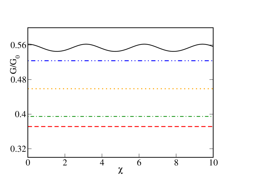
Figure 2: Plot of $G/G_{0}$ for $\delta n=0$ (black solid line), $\pm 1$ (red dashed line for $-1$ and yellow dotted line for $1$), and $\pm 2$ (green dash-dotted line for $-2$ and blue dash-double dotted line for $2$) indicating oscillatory behavior (for $\delta n=0$) or constant behavior (for $\delta n=\pm 1$ and $\pm 2$) as a function of $\chi$. For all the curves, we have chosen $n_{2}=1$ for $\delta n=0,1,2$ and $n_{1}=1$ for $\delta n=-1,-2$. Here we have set $\mu_{R}=0.5$, $\mu_{L}=\hbar v_{F}k_{F}=1$, $eV=0.2$. All energies are scaled in units of $\mu_{L}$.

To make further analytical progress, we consider the thin barrier limit in which $U_{0}\to\infty$ and $d\to 0$ keeping $\chi=U_{0}d/\hbar v_{F}$ fixed. In this limit $\theta_{2\vec{k}},k_{3z}d\to 0$ and $k_{2z}d\to\chi$. Using this one obtains from Eqs. (14)

$$r = \frac{\sin\left(\frac{\theta_{3}}{2}\right)\cos\left(\frac{\theta_{1}}{2}\right)-\sin\left(\frac{\theta_{1}}{2}\right)\cos\left(\frac{\theta_{3}}{2}\right)e^{2i\nu^{\prime}}}{\cos\left(\frac{\theta_{1}}{2}\right)\cos\left(\frac{\theta_{3}}{2}\right)e^{2i\nu^{\prime}}-\sin\left(\frac{\theta_{1}}{2}\right)\sin\left(\frac{\theta_{3}}{2}\right)},$$ (17)

where $\nu^{\prime}=(n_{1}-n_{2})\phi_{k}-\chi$. Thus we find that in this limit, for $n_{1}\neq n_{2}$, the barrier potential $\chi$ appears as a constant shift to the azimuthal angle $\phi_{k}$. Consequently, $G$ which involves a sum over all such angles becomes independent of $\chi$. In contrast, for $n_{1}=n_{2}$, $G$ is an oscillatory function of the barrier potential. These properties of $G$ in these junctions are qualitatively similar to those found in ballistic junctions of spin-half Weyl semimetals sinha1 . This behavior is numerically confirmed in Fig. 2 where $G/G_{0}$ is plotted as a function of $\chi$ for $\delta n\equiv n_{1}-n_{2}=0,\pm 1,\pm 2$. We find that $G/G_{0}$ oscillates with $\chi$ for $\delta n=0$; in contrast it is independent of $\chi$ for $\delta n\neq 0$. This independence persists for a wide range of $d$ and $U_{0}$ even when we move away from the restrictive thin barrier limit as shown in Fig. 3.

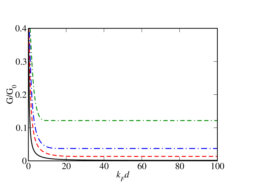
Figure 3: Plot of $G/G_{0}$ as a function of $d$ for several representative values of $U_{0}$. Here $\mu_{R}=0.5$ and all other parameters are the same as in Fig. 2. The black solid line corresponds to $\mu_{L}+eV-U_{0}=0.05$, the red dashed to $\mu_{L}+eV-U_{0}=0.15$, the blue dash-dotted to $\mu_{L}+eV-U_{0}=0.35$, and the green double dash-dotted to $\mu_{L}+eV-U_{0}=0.45$. Here $d$ is measured in units of $\hbar v_{F}/\mu_{L}=k_{F}^{-1}$ and all energies are measured in units of $\mu_{L}$.

Next, we study the $U_{0}$ dependence of the barrier potential close to $U_{0}=\mu_{L}+eV$ where we deviate significantly from the thin barrier limit for any $d$. The result is shown in Fig. 4. Remarkably, we find that $G$ vanishes for $U_{0}=\mu_{L}+eV$ for all values of $d$ and $\delta n$. The approach of $G/G_{0}$ to its zero value depends on $d$ for a given $eV$; a thicker barrier region with a larger value of $d$ leads to a more gradual decay of $G/G_{0}$ as can be seen in Fig. 4. We have also checked that this property is independent of $eV$. We note that this property is distinct from the analogous behavior of $G/G_{0}$ for two-component Dirac and Weyl fermions; for these materials $G/G_{0}$ does not approach zero for sufficiently thin barriers even if $U_{0}=\mu_{L}+eV$.

To understand this phenomenon better, we first note that for $\mu_{L}+eV-U_{0}=0$, the wave function in region $II$ must satisfy the equation

$$\sum_{a=x,y,z}S_{a}d_{an}(\vec{k})\psi_{0}(\vec{k})=0$$ (18)

for any $k_{\perp}\neq 0$ and $k_{z}$. This requires imaginary solutions for $k_{2z}=\pm i\kappa_{n}$ where $\kappa_{n}=k_{\perp}^{n}/\alpha_{n}$. This leads to evanescent modes in region $II$. The wave functions of these modes can be found by solving Eq. (18). The wave function in region $II$ is thus given by

$$|\psi^{(0)}\rangle_{II} = \frac{1}{\sqrt{3}}\Bigg{[}pe^{-\kappa_{n}z+i(k_{x}+k_{y}y-nS_{z}\phi_{k})}\begin{pmatrix}1\\ i\\ -1\end{pmatrix}$$ (19)

$$+qe^{-\kappa_{n}z+i(k_{x}+k_{y}y-nS_{z}\phi_{k})}\begin{pmatrix}-1\\ i\\ 1\end{pmatrix}\Bigg{]}.$$

The wave functions in region $I$ and $III$ do not involve $U_{0}$ and are given by Eqs. (10) and (13) respectively. Using these wave functions and matching the first and the third components of the wave function as before, we obtain

$$\cos^{2}\frac{\theta_{1\vec{k}}}{2}+r\sin^{2}\frac{\theta_{1\vec{k}}}{2}=(p-q)\sqrt{3},$$

$$\sin^{2}\frac{\theta_{1\vec{k}}}{2}+r\cos^{2}\frac{\theta_{1\vec{k}}}{2}=(q-p)/\sqrt{3},$$

$$pe^{-\kappa_{n}d}-qe^{\kappa_{n}d}=\sqrt{3}t\cos^{2}\frac{\theta_{3\vec{k}}}{2}e^{i(k_{3z}d+\nu)},$$

$$qe^{\kappa_{n}d}-pe^{-\kappa_{n}d}=\sqrt{3}t\sin^{2}\frac{\theta_{3\vec{k}}}{2}e^{i(k_{3z}d-\nu)}.$$ (20)

The only possible solution to Eqs. (20) is $r=-1$, $t=0$ and $p/q=\exp[2\kappa_{n}d]$ which indicates perfect reflection of electrons for all $k_{\perp}\neq 0$. We note that this phenomenon is independent of $d$ and $\mu_{R}$; moreover it can occur at any value of $eV$ and $\mu_{L}$ provided the condition $U_{0}=\mu_{L}+eV$ is satisfied.

In contrast, for $k_{\perp}=0$, i.e., when the particle approaches the barrier at normal incidence, the wave function in region $II$ is given by

$$|\psi^{{}^{\prime}(0)}\rangle_{II} = pe^{-\kappa_{n}z+i(k_{x}+k_{y}y-nS_{z}\phi_{k})}\begin{pmatrix}1\\ 0\\ 0\end{pmatrix}$$ (21)

$$+~{}qe^{-\kappa_{n}z+i(k_{x}+k_{y}y-nS_{z}\phi_{k})}\begin{pmatrix}0\\ 0\\ 1\end{pmatrix}.$$

Then a straightforward calculation yields $r=0$ and $t=1$ for any $d$. This is of course a manifestation of the well-known Klein tunneling. Thus we find that the barrier for $U_{0}=\mu_{L}+eV$ reflects all electrons with unit probability except the ones which are incident on it normally; the latter are transmitted with unit probability. This leads to perfect collimation in such NBN junctions. This also explains the reason for $G/G_{0}\to 0$ in this limit; $G/G_{0}$ is suppressed by a factor of $1/L^{2}$ factor since only one of the channels conduct.

When both $\Delta E\equiv\mu_{L}+eV-U_{0}$ and the angle of incidence (or, equivalently, $k_{\perp}$) are close to zero, there is a cross-over from perfect reflection to perfect transmission (Klein tunneling) as the angle of incidence approaches zero. For $\hbar v_{F}\alpha_{n_{1}}k_{\perp}^{n_{1}},\Delta E\ll(\mu_{L}+eV),(\mu_{R}+eV)$, where $\theta_{1,3}\to 0$ but $\theta_{2}$ remains finite, we find analytically that the transmission probability is given by

$$T~{}=~{}\left[1~{}+~{}\left(\frac{\hbar v_{F}d\alpha_{n_{1}}^{2}k_{\perp}^{2n_{1}}}{2\Delta E}\right)^{2}\right]^{-1}.$$ (22)

The above expression holds for any $n_{2}$ and implies that the width $\Delta E$ of the cross-over region is proportional to $d$. This explains why the width of the region of small $G/G_{0}$ in Fig. 4 decreases as $d$ becomes smaller. Using Eq. (22) and the Jacobian $J_{0}$ in Eq. (16) to integrate over $\theta_{1}$, we find that $G/G_{0}\sim(\Delta E/d)^{1/n_{1}}$ for $\Delta E\ll(\mu_{L}+eV)$. In principle, this scaling form gives a way of experimentally measuring the value of $n_{1}$, although it may be very hard to study the region of small $\Delta E$ since $G$ would be small in this regime.

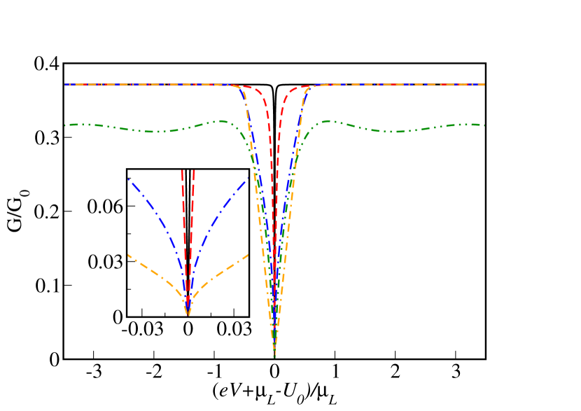
Figure 4: Plot of $G/G_{0}$ as a function of $\mu_{L}+eV-U_{0}$ for several values of $\delta n$ and $d$, with a fixed applied voltage $eV=0.2$ and chemical potentials $\mu_{L}=1$ and $\mu_{R}=0.5$. The green dotted line corresponds to $dk_{F}=1$ and $\delta n=0$. The orange double dash-dotted, the blue dash-dotted, the red dash-dotted and the black solid lines correspond to $\delta n=-1$ and $dk_{F}=50$, $dk_{F}=5$, $dk_{F}=1$ and $dk_{F}=0.5$ respectively. The convention for choosing $n_{1}$ and $n_{2}$ for a given $\delta n$ is the same as in Fig. 2. All energies are in units of $\mu_{L}$. The inset presents a closer view of $G/G_{0}$ around $\mu_{L}+eV-U_{0}=0$.

Before ending the discussion of the collimation effect, we would like to note that this is rather unique to integer pseudospin fermion systems since it can only occur in a system where current conservation does not enforce continuity of the entire wave function. This can be seen by noting that the fermion wave function in region $III$, $|\psi\rangle_{III}$, vanishes for any $k_{\perp}\neq 0$ since $t=0$ for $\mu_{L}+eV=U_{0}$. In contrast, in region $II$ the wave function $|\psi^{(0)}\rangle_{II}$ is finite and is given by Eq. (19) with $p/q=\exp[2\kappa d]$. Thus this solution necessarily requires a wave function discontinuity at $z=d$. Also, it is easy to see using similar analysis that for hole mediated transport an analogous collimation would occur at $U_{0}=\mu_{L}-eV$.

We now turn to an opposite effect called super-Klein tunneling xu . For $U_{0}=2(\mu_{L}+eV)$, we find from Eqs. (14) that the transmission probability for a given incident momentum $\vec{k}$ is given by

$$T~{}=~{}\frac{4\cos\theta_{1\vec{k}}\cos\theta_{3\vec{k}}}{(\cos\theta_{1\vec{k}}+\cos\theta_{3\vec{k}})^{2}~{}+~{}4\sin^{2}\nu\sin^{2}\theta_{1\vec{k}}\sin^{2}\theta_{3\vec{k}}}.$$ (23)

We now see that if $n_{1}=n_{2}$ and $\mu_{L}=\mu_{R}$, $T=1$ for all values of $\theta_{1\vec{k}}$; this is called super-Klein tunneling. However, we see that this phenomenon does not occur if either $n_{1}\neq n_{2}$ or $\mu_{L}\neq\mu_{R}$.

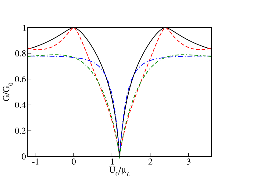
Figure 5: Plot of $G/G_{0}$ as a function of $U_{0}$ for several values of $\delta n$ and $d$, with a fixed applied voltage $eV=0.2$ and chemical potentials $\mu_{L}=\mu_{R}=1$. The black solid, red dashed, blue dash-dotted and green double dash-dotted lines correspond to $(dk_{F},\delta n)$ equal to $(0.5,0),~{}(1,0),~{}(0.5,-1)$ and $(1,-1)$ respectively. The convention for choosing $n_{1}$ and $n_{2}$ for a given $\delta n$ is the same as in Fig. 2. All energies are in units of $\mu_{L}$.

Finally, we would like to point out a remarkable symmetry of the conductance as a function of $U_{0}$ for any value of $d$ and $\delta n$, namely, that $G/G_{0}$ has the same value at two values of the barrier potential $U_{0}$ which are related to each other by reflection about the value $\mu_{L}+eV$. This is clearly visible in Fig. 5 where $\mu_{L}+eV=1.2$; reflection about $\mu_{L}+eV$ then corresponds to the values $U_{0}$ and $2.4-U_{0}$. To show this symmetry, suppose that Eqs. (14) describe the various amplitudes for a value $U_{0}$. Then we find that at $2(\mu_{L}+eV)-U_{0}$, the corresponding equations (with amplitudes denoted by primes) are given by

$$\cos^{2}\frac{\theta_{1\vec{k}}}{2}~{}+~{}r^{\prime}\sin^{2}\frac{\theta_{1\vec{k}}}{2} = q^{\prime}\cos^{2}\frac{\theta_{2\vec{k}}}{2}~{}+~{}p^{\prime}\sin^{2}\frac{\theta_{2\vec{k}}}{2},$$ (24)

$$\sin^{2}\frac{\theta_{1\vec{k}}}{2}~{}+~{}r^{\prime}\cos^{2}\frac{\theta_{1\vec{k}}}{2} = q^{\prime}\sin^{2}\frac{\theta_{2\vec{k}}}{2}~{}+~{}p^{\prime}\cos^{2}\frac{\theta_{2\vec{k}}}{2},$$

$$q^{\prime}\cos^{2}\frac{\theta_{2\vec{k}}}{2}e^{ik_{2z}d}~{}+~{}p^{\prime}\sin^{2}\frac{\theta_{2\vec{k}}}{2}e^{-ik_{2z}d} = t^{\prime}\cos^{2}\frac{\theta_{3\vec{k}}}{2}e^{i(k_{3z}d+\nu^{\prime})},$$

$$q^{\prime}\sin^{2}\frac{\theta_{2\vec{k}}}{2}e^{ik_{2z}d}~{}+~{}p^{\prime}\cos^{2}\frac{\theta_{2\vec{k}}}{2}e^{-ik_{2z}d} = t^{\prime}\sin^{2}\frac{\theta_{3\vec{k}}}{2}e^{i(k_{3z}d-\nu^{\prime})}.$$

We now observe that complex conjugating Eqs. (14) precisely give Eqs. (24) if we take $p^{\prime}=q^{*}$, $q^{\prime}=p^{*}$, $r^{\prime}=r^{*}$, $t^{\prime}=t^{*}e^{-i2k_{3z}d}$, and $\nu^{\prime}=-\nu$. These relations mean that the transmission probability is the same (i.e., $1-|r|^{2}=1-|r^{\prime}|^{2}$) for the values $U_{0}$ and angle $\phi_{\vec{k}}$ and the values $2(\mu_{L}+eV)-U_{0}$ and angle $-\phi_{\vec{k}}$. Since the conductance is calculated by integrating over all angles $\phi_{\vec{k}}$ from 0 to $2\pi$ (equivalently, from $-\pi$ to $\pi$), we see that the conductance will be the same for $U_{0}$ and $2(\mu_{L}+eV)-U_{0}$. Clearly, this argument holds for any value of $d$ and $\delta n$. Also, it is easy to see that identical arguments would hold for hole mediated transport; however, in that case, $G$ would be invariant under $U_{0}\to 2(\mu_{L}-eV)-U_{0}$.

III NBS junction

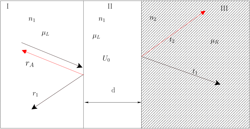
Figure 6: Schematic picture of a ballistic NBS junction with a proximate superconductor (not shown in the figure) atop region $III$ (shaded region). The longitudinal coordinate is $z$ and the barrier region (region $II$) with a potential $U_{0}$ has a width $d$ along $z$. $\mu_{L}$ and $\mu_{R}$ denote the chemical potentials in regions $I$ and $III$ respectively. The figure shows the amplitudes of both normal ($r$) and Andreev reflections ($r_{A}$) in region I. $t_{1}$ and $t_{2}$ denotes the amplitudes of electron- and hole-like quasiparticles in the superconducting region.

In this section, we will study transport through a NBS junction which hosts pseudospin-one fermions. A schematic picture of the proposed setup is shown in Fig. 6. In what follows, we assume that superconductivity is induced in region $III$ by a proximate $s$-wave superconductor leading to the induction of a $s$-wave pair potential between two Weyl nodes $A$ and $B$. We note that several possibilities of unconventional (i.e., non-$s$-wave) superconductivity have recently been proposed as possible phases of pseudospin-one fermion systems lin1 ; however, in this work we will assume $s$-wave symmetry. The Hamiltonian of the system in the presence of such $s$-wave pairing in region $III$ is given by

$$H_{s} = \sum_{\vec{k}}~{}\psi_{\vec{k}}^{\dagger}~{}[\tau_{z}(H_{n_{2}}(\vec{k})-\mu_{R})+\tau_{x}\Delta]~{}\psi_{\vec{k}}$$ (25)

$$= \sum_{\vec{k}}~{}\psi_{\vec{k}}^{\dagger}H_{s}(\vec{k})\psi_{\vec{k}},$$

where $H_{n_{2}}(\vec{k})$ is the normal state Hamiltonian defined in Eq. (1), $\tau_{z,x}$ are spin-half Pauli matrices in particle-hole space, and $\psi_{\vec{k}}$ is a six-component spinor field whose top three components represent pseudospin-one electron wave functions at Weyl node $A$ while the bottom three components represent hole wave functions at node $B$. The eigenfunctions corresponding to right-moving electron- and hole-like quasiparticles obtained by solving $H_{s}(\vec{k})\psi_{\vec{3}k}=(\mu_{R}+eV)\psi_{\vec{k}}$ are given by

$$\psi_{3e}^{s} = e^{i(k_{3z}z+k_{x}x+k_{y}y)}\exp[-iS_{z}\phi_{\vec{k}}]\left(e^{i\beta}\cos^{2}\frac{\theta_{3}}{2},e^{i\beta}\frac{\sin\theta_{3}}{\sqrt{2}},e^{i\beta}\sin^{2}\frac{\theta_{3}}{2},\cos^{2}\frac{\theta_{3}}{2},\frac{\sin\theta_{3}}{\sqrt{2}},\sin^{2}\frac{\theta_{3}}{2}\right),$$

$$\psi_{3h}^{s} = e^{-i(k^{\prime}_{3z}z+k_{x}x+k_{y}y)}\exp[-iS_{z}\phi_{\vec{k}}]\left(\sin^{2}\frac{\theta_{3}^{\prime}}{2},\frac{\sin\theta_{3}^{\prime}}{\sqrt{2}},\cos^{2}\frac{\theta_{3}^{\prime}}{2},e^{i\beta}\sin^{2}\frac{\theta_{3}^{\prime}}{2},e^{i\beta}\frac{\sin\theta_{3}^{\prime}}{\sqrt{2}},e^{i\beta}\cos^{2}\frac{\theta_{3}^{\prime}}{2}\right),$$ (26)

where $\theta_{3}(\theta_{3}^{\prime})=\arctan[\alpha_{n_{2}}k_{\perp}^{n_{2}}/k_{3e}^{z+}(k_{3h}^{z+})]$ and $k_{3z}(k^{\prime}_{3z})=\sqrt{(\mu_{R}+(-)\Omega)^{2}-\alpha_{n_{2}}^{2}k_{\perp}^{2n_{2}}}$. Here for $eV>\Delta$, we have $\Omega=[(eV)^{2}-\Delta^{2}]^{1/2}$ and $\beta=-i{\rm arccosh}(eV/\Delta)$ whereas, for $eV<\Delta$, $\Omega=i[\Delta^{2}-(eV)^{2}]^{1/2}$ and $\beta=\arccos(eV/\Delta)$. In what follows, we will set the phase of the superconductor pair potential to be zero and omit the $\vec{k}$ index for $\theta_{3}$, $\theta^{\prime}_{3}$ and $\beta$ for clarity.

In region $I$, $\Delta=0$, and electron (hole) wave functions can be obtained from solution of $\pm H_{n_{1}}(\vec{k})\psi=(eV\pm\mu_{L})\psi$. We note that in region $I$, corresponding to a right-moving incident electron on the barrier at $z=0$, there is a reflected left-moving electron and an Andreev reflected left-moving hole. The wave functions of these electrons and holes are given by

$$\psi_{1R}^{e} = e^{i(k_{1z}z+k_{x}x+k_{y}y)}\exp[-in_{1}S_{z}\phi_{k}]\left(\cos^{2}(\theta_{1}/2),\sin(\theta_{1})/\sqrt{2},\sin^{2}(\theta_{1})/2,0,0,0\right),$$

$$\psi_{1L}^{e} = e^{i(-k_{1z}z+k_{x}x+k_{y}y)}\exp[-in_{1}S_{z}\phi_{k}]\left(\sin^{2}(\theta_{1}/2),\sin(\theta_{1})/\sqrt{2},\cos^{2}(\theta_{1})/2,0,0,0\right),$$

$$\psi_{1L}^{h} = e^{i(-k^{\prime}_{1z}z+k_{x}x+k_{y}y)}\exp[-in_{1}S_{z}\phi_{k}]\left(0,0,0,\cos^{2}(\theta^{\prime}_{1}/2),-\sin(\theta^{\prime}_{1})/\sqrt{2},\sin^{2}(\theta^{\prime}_{1})/2\right),$$ (27)

where $\theta_{1}=\arcsin[\alpha_{n_{1}}k^{n_{1}}_{\perp}/|\mu_{L}+eV|]$, $\theta_{1}^{\prime}=\arcsin[-\sin\theta_{1}|\mu_{L}+eV|/|\mu_{L}-eV|]$, $k_{1z}=(\mu_{L}+eV)\cos\theta_{1}$, and $k^{\prime}_{1z}=(eV-\mu_{L})\cos\theta_{1}^{\prime}$. The wave function in region $I$ is thus given by

$$\psi_{I}^{s} = \psi_{1R}^{e}+r\psi_{1L}^{e}+r_{A}\psi_{1L}^{h},$$ (28)

where $r(r_{A})$ is the amplitude of normal (Andreev) reflection from the barrier.

Similarly, in region $II$ the wave function consists of a linear superposition of left- and right-moving electron and hole wave functions. The wave functions for right- and left-moving electrons and that of the left-moving hole are denoted by $\psi_{2R}^{e}$, $\psi_{2L}^{e}$, and $\psi_{2L}^{h}$ respectively. Their expressions can be read off from Eqs. (27) with

$$\theta_{1}\to\theta_{2}=\arcsin[\alpha_{n_{1}}k^{n_{1}}_{\perp}/|\mu_{L}+eV-U_{0}|,$$

$$\theta^{\prime}_{1}\to\theta^{\prime}_{2}=\arcsin\left[-\sin\theta_{2}\frac{|\mu_{L}+eV-U_{0}|}{|\mu_{L}-eV-U_{0}|}\right],$$

$$k_{1z}\to k_{2z}=(\mu_{L}+eV-U_{0})\cos\theta_{2},$$

$$k^{\prime}_{1z}\to k^{\prime}_{2z}=(eV-\mu_{L}+U_{0})\cos\theta_{2}^{\prime}.$$ (29)

The wave function of the right-moving hole in region $II$ is given by

$$\psi_{2R}^{h} = e^{i(k^{\prime}_{2z}z+k_{x}x+k_{y}y)}\exp[-in_{1}S_{z}\phi_{k}]$$

$$\times\left(0,0,0,\sin^{2}(\theta^{\prime}_{2}/2),-\sin(\theta^{\prime}_{2})/\sqrt{2},\cos^{2}(\theta^{\prime}_{2})/2\right).$$

The wave function in region $II$ can be written as a superposition of these wave functions as

$$\psi_{II}^{s} = p_{1}\psi_{2R}^{e}+q_{1}\psi_{2L}^{e}+p_{2}\psi_{2L}^{h}+q_{2}\psi_{2R}^{h}.$$ (31)

The wave function in region $III$ can be written as a linear superposition of electron- and hole-like quasiparticle wave functions given in Eq. (26) and are given by

$$\psi_{III} = t_{1}\psi_{3e}^{s}+t_{2}\psi_{3h}^{s}.$$ (32)

Here $t_{1}$ and $t_{2}$ denotes amplitudes of electron- and hole-like quasiparticles in $\psi_{III}$ respectively.

To compute the conductance $G$ of the NBS junction, we first need to determine the coefficients $r$ and $r_{A}$. To this end, we demand current conservation at $z=0$ and $z=d$. We find that similar to the NBN junction, the current through NBS junctions of pseudospin-one fermions do not involve all the components of the wave function; consequently, the conservation does not necessitate continuity of the entire wave function across the boundaries between region $I$ and $II$ and between $II$ and $III$. We note that for NBS junctions hosting integer pseudospin $s$ fermions with $4s+2$ component wave functions, only $4s$ components of the wave function would be continuous. Moreover, it is easy to see from Eqs. (26) and (27) that current conservation along $z$ does not involve the second and the fifth components of the wave functions in regions $I$, $II$ and $III$. Thus we enforce the current conservation along $z$ by only demanding continuity of the other four components of the wave function. The procedure is similar to that charted out for NBN junctions and yields, at $z=0$,

$$\cos^{2}(\theta_{1}/2)+r\sin^{2}(\theta_{1}/2) = p_{1}\cos^{2}(\theta_{2}/2)+q_{1}\sin^{2}(\theta_{2}/2),$$

$$\sin^{2}(\theta_{1}/2)+r\cos^{2}(\theta_{1}/2) = p_{1}\sin^{2}(\theta_{2}/2)+q_{1}\cos^{2}(\theta_{2}/2),$$

$$r_{A}\cos^{2}(\theta^{\prime}_{1}/2) = p_{2}\cos^{2}(\theta^{\prime}_{2}/2)+q_{2}\sin^{2}(\theta^{\prime}_{2}/2),$$

$$r_{A}\sin^{2}(\theta^{\prime}_{1}/2) = p_{2}\sin^{2}(\theta^{\prime}_{2}/2)+q_{2}\cos^{2}(\theta^{\prime}_{2}/2).$$

Similarly, at $z=d$ one obtains

$$p_{1}\cos^{2}(\theta_{2}/2)e^{ik_{2z}d}+q_{1}\sin^{2}(\theta_{2}/2)e^{-ik_{2z}d}$$

$$=[t_{1}e^{i(\beta+k_{3z}d)}\cos^{2}(\theta_{3}/2)+t_{2}e^{-ik^{\prime}_{3z}d}\sin^{2}(\theta^{\prime}_{3}/2)]e^{i\nu^{\prime}},$$

$$p_{1}\sin^{2}(\theta_{2}/2)e^{ik_{2z}d}+q_{1}\cos^{2}(\theta_{2}/2)e^{-ik_{2z}d}$$

$$=[t_{1}e^{i(\beta+k_{3z}d)}\sin^{2}(\theta_{3}/2)+t_{2}e^{-ik^{\prime}_{3z}d}\cos^{2}(\theta^{\prime}_{3}/2)]e^{-i\nu^{\prime}},$$

$$p_{2}\cos^{2}(\theta^{\prime}_{2}/2)e^{-ik^{\prime}_{2z}d}+q_{2}\sin^{2}(\theta^{\prime}_{2}/2)e^{ik^{\prime}_{2z}d}$$ (34)

$$=[t_{1}e^{ik_{3z}d}\cos^{2}(\theta_{3}/2)+t_{2}e^{-i(k^{\prime}_{3z}d-\beta)}\sin^{2}(\theta^{\prime}_{3}/2)]e^{i\nu^{\prime}},$$

$$p_{2}\sin^{2}(\theta^{\prime}_{2}/2)e^{-ik^{\prime}_{2z}d}+q_{2}\cos^{2}(\theta^{\prime}_{2}/2)e^{ik^{\prime}_{2z}d}$$

$$=[t_{1}e^{ik_{3z}d}\sin^{2}(\theta_{3}/2)+t_{2}e^{-i(k^{\prime}_{3z}d-\beta)}\cos^{2}(\theta^{\prime}_{3}/2)]e^{-i\nu^{\prime}},$$

where $\nu^{\prime}=(n_{1}-n_{2})\phi_{k}$. From Eqs. (III) and (34) we solve numerically for $r$ and $r_{A}$. The conductance $G$ is then obtained from the usual Landauer-Buttiker approach btk1

$$G_{s}(eV) = G_{N}\int d^{2}k\,T_{s},\quad T_{s}=(1-|r|^{2}+|r_{A}|^{2}),$$

where $G_{N}=n_{0}e^{2}(k_{F}L)^{2}/h$ is the normal state conductance of region $I$, where $k_{F}=\mu_{L}+eV/\hbar v_{F}$, and we have chosen $n_{1}=1$. We note here that the range of the integration over the transverse momentum $(k_{x},k_{y})$ in Eq. (LABEL:supcondcal) is determined by demanding that $\theta_{1,2}$ and $\theta^{\prime}_{1,2}$ in regions I and II have real solutions ks1 .

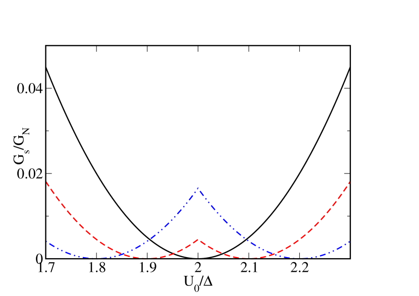
Figure 7: Plot of $G_{s}/G_{N}$ as a function of $U_{0}$ for $\mu_{L}=\mu_{R}=2$, $n_{1}=1$, $n_{2}=2$, and $\Delta=1$. The black dash-dotted line corresponds to $eV=0$, the red dashed line to $eV=0.1$, and the blue solid line to $eV=0.2$. The dips in $G_{s}$ occur when $U_{0}=\mu_{L}+eV$ or $U_{0}=\mu_{L}-eV$. All energies are scaled in units of $\Delta$ and $dk_{F}=1$ for all plots.

We will first study the subgap conductance $G_{s}(eV)$ as a function of $U_{0}$ near $U_{0}=\mu_{L}+eV$. We note that in the NBN junction when $U_{0}$ is tuned to this value, it led to collimation and a consequent suppression of $G$. We find a similar suppression of $G(eV)$ as shown in Fig. 7. We find that $G_{s}(eV)\simeq 0$ for $U_{0}=\mu_{L}+eV$ and its approach to zero as $U_{0}\to\mu_{L}+eV$ is controlled by the thickness $d$ of the barrier region (similar to the discussion around Eq. (22) for a NBN junction). This behavior can be understood by noting that for $k_{\perp}\neq 0$ and $U_{0}=\mu_{L}+eV$, the right- and the left-moving electron wave functions in region $II$ are given by Eq. (19). Thus the first two equations in Eqs. (III) reduce to the first two equations in Eqs. (20); they lead to a solution $r=-1$. Similarly the first two equations in Eq. (34) can be shown to lead to the solution $t_{1}=t_{2}=0$, similar to that found in last two equations in Eqs. (20). This forces $p_{2}=q_{2}=r_{A}=0$ leading to a complete suppression of transmission for any non-zero angle of incidence. This feature is reflected in the dips at $U_{0}=\mu_{L}+eV$ (at $U_{0}/\Delta=2,\,2.1,\,2.2$) in Fig. 7. A similar argument can be given for $U_{0}=\mu_{L}-eV$ by considering a hole approaching the barrier leading to a reflected hole with amplitude $r$ and an Andreev reflected electron with amplitude $r_{A}$. Once again a similar calculation to the one carried out above shows that $r=-1$ and $r_{A}=0$ for $U_{0}=\mu_{L}-eV$. This leads to the dips in $G_{s}$ for $U_{0}=\mu_{L}-eV$ at $U_{0}/\Delta=2,\,1.9,\,1.8$. These dips therefore constitute a concrete signature of collimation in the subgap tunneling conductance of such NBS junctions.

We note that Fig. 7 seems to indicate that $G_{s}$ is reflection symmetric about $U_{0}=\mu_{L}$. This is however only an approximate symmetry which can be understood as follows. We first note that in the parameter regime where $eV\ll\mu_{L}$ and $U_{0}$, $G_{s}$ receives contributions from only near-normal angles of incidence. Indeed, in all the curves in Fig. 8, the maximum angle of incidence for which the channels conduct is given by $\theta^{\rm max}\leq 0.15$, and $\theta_{1},\theta^{\prime}_{1}\leq\theta^{\rm max}$. Thus we can replace $\cos(\theta_{1}/2),\cos(\theta^{\prime}_{1}/2)\to 1$ and $\sin(\theta_{1}/2),\sin(\theta^{\prime}_{1}/2)\to 0$ in Eqs. (III). This leads to

$$1 \simeq p_{1}\cos^{2}(\theta_{2}/2)+q_{1}\sin^{2}(\theta_{2}/2),$$

$$r \simeq p_{1}\sin^{2}(\theta_{2}/2)+q_{1}\cos^{2}(\theta_{2}/2),$$

$$r_{A} \simeq p_{2}\cos^{2}(\theta^{\prime}_{2}/2)+q_{2}\sin^{2}(\theta^{\prime}_{2}/2),$$

$$0 \simeq p_{2}\sin^{2}(\theta^{\prime}_{2}/2)+q_{2}\cos^{2}(\theta^{\prime}_{2}/2).$$ (36)

Moreover, in this regime we numerically find that $r_{A}\simeq 1$ and $r\simeq 0$ for all $\theta_{1}$.

Next, we consider a change of $U_{0}=\mu_{L}+\delta$ to $U_{0}=\mu_{L}-\delta$ for an arbitrary small value of $\delta$ and a fixed applied bias voltage $eV$. Using Eqs. (27) and (29), it is easy to see that under such a transformation $\theta_{2}\Leftrightarrow\theta^{\prime}_{2}$ and $k_{z2}\Leftrightarrow k^{\prime}_{z2}$. Thus, as long as $r\simeq 0$, and $r_{A}\simeq 1$, Eqs. (36) is approximately invariant under this transformation with $p_{1}\to p^{\prime}_{1}=p_{2}^{\ast}$, $q_{1}\to q_{1}^{\prime}=q_{2}^{\ast}$, $r\to r^{\prime}=r^{\ast}$, and $r_{A}\to r^{\prime}_{A}=r_{A}^{\ast}$. Moreover, it is easy to see that the same transformation keeps Eq. (34) invariant with $t_{1}\to t^{\prime}_{1}=t_{1}^{\ast}e^{-i\beta}$, $t_{2}\to t^{\prime}_{2}=t_{2}^{\ast}e^{i\beta}$ and $\nu\to\nu^{\prime}=-\nu$. Thus the transmission probabilities and hence the conductance $G_{s}$ (which is computed by integrating over the azimuthal angle and is hence invariant under the change $\nu\to-\nu$) remains approximately invariant under this transformation. We note that, in contrast to the conductance of NBN junctions, the invariance for $G_{s}$ is approximate and holds only for $\theta_{1},\theta^{\prime}_{1}\to 0$ for which $r_{A}\simeq 0$ and $r\simeq 1$.

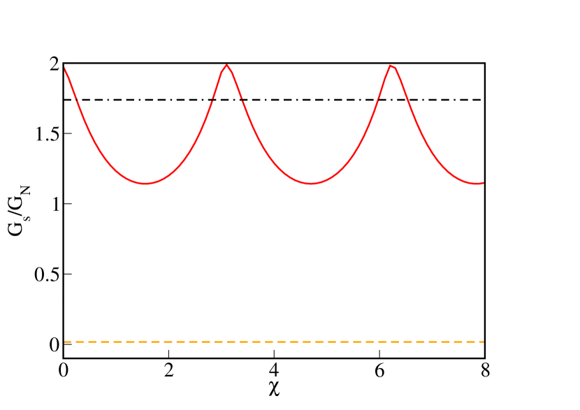
Figure 8: Plot of the zero-bias tunneling conductance $G_{s}(0)/G_{N}$ as a function of $\chi$ for $eV=0,~{}\mu_{L}=\mu_{R}=100$ and $\Delta=1$. All energies are scaled in units of $\Delta$. The red solid line corresponds to $\delta n=0$, the yellow dashed line to $\delta n=-1$, and the black dash-dotted line to $\delta n=1$. The convention for choosing $n_{1}$ and $n_{2}$ for a given $\delta n$ is the same as in Fig. 2.

Finally, we study the dependence of the subgap tunneling conductance on the barrier strength $\chi$ in the thin barrier limit. In this limit $\theta_{2},\theta^{\prime}_{2},k_{3z}d,k^{\prime}_{3zd}\to 0$ and $k_{2z}d,k^{\prime}_{2z}d\to\chi=U_{0}d/\hbar v_{F}$. Substituting this in Eqs. (III) and (34), we obtain

$$\cos^{2}(\theta_{1}/2)+r\sin^{2}(\theta_{1}/2) = p_{1}=[t_{1}e^{i\beta}\cos^{2}(\theta_{3}/2)+t_{2}\sin^{2}(\theta_{3}/2)]e^{i\nu},$$

$$\sin^{2}(\theta_{1}/2)+r\cos^{2}(\theta_{1}/2) = q_{1}=[t_{1}e^{i\beta}\sin^{2}(\theta_{3}/2)+t_{2}\cos^{2}(\theta^{\prime}_{3}/2)]e^{-i\nu},$$

$$r_{A}\cos^{2}(\theta^{\prime}_{1}/2) = p_{2}=[t_{1}\cos^{2}(\theta_{3}/2)+t_{2}e^{i\beta}\sin^{2}(\theta^{\prime}_{3}/2)]e^{i\nu},$$

$$r_{A}\sin^{2}(\theta^{\prime}_{1}/2) = q_{2}=[t_{1}\sin^{2}(\theta_{3}/2)+t_{2}e^{i\beta}\cos^{2}(\theta^{\prime}_{3}/2)]e^{-i\nu},$$ (37)

where $\nu=(n_{1}-n_{2})\phi_{\vec{k}}-\chi$. These equations can be solved to obtain the expression for $r$ and $r_{A}$. We note here that $\chi$ enters these equations only as a constant shift to the azimuthal angle $\phi_{\vec{k}}$. This ensures that $G_{s}$, similar to its counterparts in spin-half Weyl and multi-Weyl semimetals, will be an oscillatory function of the barrier strength $\chi$ if $n_{1}=n_{2}$; in contrast, for $n_{1}\neq n_{2}$, $G_{s}$ becomes independent of $\chi$ in the thin barrier limit. This behavior is shown in Fig. 8.

IV Discussion

In this work, we have studied the transport properties of pseudospin-one fermions in the presence of a potential barrier. Such fermion systems host quasiparticles which obey an effective spin-one Dirac equation. Thus transport in NBN and NBS junctions show unconventional features which are absent in similar junctions of both conventional (Schrödinger) metals and pseudospin/spin-half Weyl semimetals.

One of the key features of ballistic transport in junctions hosting pseudospin-one fermion is that for these junctions, current conservation does not require continuity of all components of the wave function across the junction. This feature can be contrasted with Schrödinger materials where conservation current enforces continuity of both the entire wave function and its derivative and spin-half Dirac/Weyl semimetals where it enforces continuity of the entire wave function. We show that this is a natural consequence of the non-invertibility of the spin matrices $S_{\alpha}$ which generate the spin/pseudospin algebra. This property is therefore expected to hold for all integer spin/pseudospin Weyl systems where the expression for the current $J_{\alpha}$ does not involve all the components of the fermion wave function; indeed, for an integer spin $s$ Weyl fermion, one requires continuity of only $2s$ components of the wave function. This features allows for current conservation without imposing constraints on all components of the fermion wave function.

The most notable consequence of the discontinuity in some components of the wave function is the collimation properties of transport through such junctions. It is well-known that pseudospin-one electromagnetic waves with effective Dirac-like dispersion may show such a collimation in the presence of an array of potential barriers fang1 ; however, here we demonstrate perfect collimation for a single barrier. We show that for both NBN and NBS junctions of these materials, the transport is collimated for a specific value of the barrier potential. It can be analytically shown that any fermion that approaches the barrier of a NBN junction with energy $\mu_{L}+eV$ at a finite angle of incidence gets reflected off the barrier with unit probability if $U_{0}=\mu_{L}+eV$. In contrast, a fermion approaching the barrier at normal incidence is transmitted with unit probability. Since the latter effect is a manifestation of Klein tunneling, this makes these systems interesting platforms for observing Klein tunneling through transport experiments. Similar effect occur for hole mediated transport for $U_{0}=\mu_{L}-eV$. We also note that the NBN junctions hosting pseudospin-one fermion system exhibit an interesting symmetry of the conductance, namely, $G$ is the same for two values of $U_{0}$ which are related to each other by reflection about the value $\mu_{L}+(-)eV$ provided that the transport occurs via motion of electron (hole)-like quasiparticles.

For NBS junctions, since the transport involves both electrons and holes, such dips in the conductance signifying collimation is seen for both $U_{0}=\mu_{L}+eV$ and $U_{0}=\mu_{L}-eV$. Such collimation does not occur in spin-half Dirac/Weyl systems since, as shown in Sec. II, it requires a discontinuity of the fermion wave function across the junction and can thus occur only for junctions hosting integer pseudospin Dirac fermions for which current conservation does not enforce continuity of the entire wave function. We also note that for these junctions, where the transport is mediated by both electron- and hole-like quasiparticles, $G_{s}$ is, in general, not invariant under $U_{0}\to 2(\mu_{L}\pm eV)-U_{0}$ for any finite $V$. This is a consequence of the participation of both electron- and hole-like quasiparticles in transport. However, we find that in the regime where $eV\ll\mu_{L}$ and $U_{0}$, only channels corresponding to near-normal incidence of the electrons contribute to $G_{s}$. In this regime, $r\simeq 0$ and $r_{A}\simeq 1$ and the subgap tunneling conductance $G_{s}$ can be shown to have an approximate invariance under the transformation of $U_{0}=\mu_{L}+\delta$ to $U^{\prime}_{0}=\mu_{L}-\delta$ for any fixed applied voltage. Thus a plot of $G_{s}$ as a function of $U_{0}$ appears to be almost reflection symmetric about $\mu_{L}$ as shown in Fig. 7.

In contrast, the barrier potential dependence of spin-one Weyl fermions is qualitatively similar to its spin-half Weyl counterpart in the thin barrier limit  sinha1 . We find that in this limit, the tunneling conductance of NBN and NBS junctions of these materials oscillates with $\chi$ for $n_{1}=n_{2}$; in contrast, they become independent of $\chi$ if $n_{1}\neq n_{2}$. The latter phenomenon, also seen for a junction between spin-half Weyl and multi-Weyl semimetals, constitutes a signature of the change in the topological winding number of the system across the junction sinha1 .

We note that our theoretical predictions can be easily tested in experiments. Several materials are expected to be candidates for pseudospin-one fermions crystalrefs . We predict that a NBN junction of these materials will show dips in tunneling conductance when the barrier potential is tuned to $\mu_{L}+eV$ (for electron transport) or to $\mu_{L}-eV$ (for hole transport). Moreover, we also expect $G/G_{0}$ to be identical for barrier potential values $U_{0}$ and $2(\mu_{L}+(-)eV)-U_{0}$, where $+(-)$ sign is applicable for electron (hole) mediated transport. To realize this behavior experimentally, one needs, for electron transport, to apply a potential $U_{0}$ which is close to $\mu_{L}$; thus these experiments would be easier to perform in systems where the Fermi energy of the pseudospin-one fermions is close to the Weyl nodes. In this context, we also note that our theoretical analysis has been carried out in the ballistic regime and assuming that there is no internode scattering between the Weyl fermions. The former can be justified by noting that in these systems (as shown for spin-half Weyl and two-dimensional Dirac systems in Ref. disorder1, ), there is usually always a quasi-ballistic regime at weak disorder where the analysis of the ballistic junctions holds. The latter approximation can be justified by noting that internode scattering is usually suppressed at low energies internode1 ; moreover, they can only occur if the two Weyl nodes occur at the same transverse momentum since scattering from the barrier must conserve momentum.

In conclusion, we have studied ballistic transport in NBN and NBS junctions of pseudospin-one Weyl fermions. We have shown that current conservation in such junctions does not require continuity of the entire fermion wave function. We have identified this property to be the reason for perfect collimation in such junctions at specific values of the barrier potential. We have discussed experiments which can test our theory.

Acknowledgments

S.N. thanks D. Sinha for useful discussions. K.S. thanks J.D. Sau for discussions. D.S. thanks DST, India for Project No. SR/S2/JCB-44/2010 for financial support.

References

(1)
(2) A. H. Castro Neto and A. Geim, Rev. Mod. Phys. 81, 109 (2009);
M. Z. Hasan and C. L. Kane, Rev. Mod. Phys. 82, 3045 (2010); X.-L. Qi
and S.-C. Zhang, Rev. Mod. Phys. 83, 1057 (2011); N. P. Armitage,
E. J. Mele, and A. Vishwanath, Rev. Mod. Phys. 90, 015001 (2018);
(3) W. Witczak-Krempa, G. Chen, Y. B. Kim, and L. Balents,
Annu. Rev. Condens. Matter Phys. 5, 57 (2014). B. Yan and C. Felser,
Annu. Rev. Condens. Matter Phys. 8, 337 (2017); M. Z. Hasan, S.-Y. Xu,
I. Belopolski and S.-M. Huang, ibid8, 289 (2017);
S. Rao, arXiv:1603.02821.
(4) X. Wan, A. M. Turner, A. Vishwanath, and S. Y. Savrasov,
Phys. Rev. B 83, 205101 (2011); A. A. Burkov and L. Balents, Phys. Rev.
Lett. 107, 127205 (2011); A. A. Burkov, M. D. Hook, and L. Balents,
Phys. Rev. B 84, 235126 (2011); G. Xu, H. Weng, Z. Wang, X. Dai, and
Z. Fang, Phys. Rev. Lett. 107, 186806 (2011); P. Hosur,
S. A. Parameswaran, and A. Vishwanath, Phys. Rev. Lett. 108, 046602
(2012); E.-G. Moon, C. Xu, Y. B. Kim, and L. Balents, Phys. Rev. Lett. 111, 206401
(2013).
(5) S.-Y. Xu et al., Science 349, 613 (2015);
B. Q. Lv et al., Phys. Rev. X 5, 031013 (2015); A. A. Burkov,
J. Phys. Condens. Matter 27, 113201 (2015); A. Turner and A. Vishwanath,
arXiv:1301.0330; P. Hosur and X. Qi, Comptes Rendus Physique, 14, 857
(2013); A. G. Grushin, Phys. Rev. D 86, 045001 (2012); D. T. Son and N.
Yamamoto, Phys. Rev. Lett. 109, 181602 (2012); A. Zyuzin and A. Burkov,
Phys. Rev. B 86, 115133 (2012); A. Zyuzin, S. Wu, and A. Burkov,
Phys. Rev. B 85, 165110 (2012); U. Khanna, A. Kundu and S. Rao, Phys. Rev. B95, 201115 (R) (2017); U. Khanna, D. K. Mukherjee, A. Kundu and S. Rao,
Phys. Rev. B93, 121409(R) (2016).
(6) A. A. Zyuzin and A. A. Burkov, Phys. Rev. B 86, 115133
(2012); M. N. Chernodub, A. Cortijo, A. G. Grushin, K. Landsteiner, and
M. A. Vozmediano, Phys. Rev. B 89, 081407 (2014); Z. Jian-Hui, J. Hua,
N. Qian, and S. Jun-Ren, Chinese Phys. Lett. 30, 027101 (2013);
A. Burkov, J. Phys. Condens. Matter 27, 113201 (2015); J. Ma and
D. A. Pesin, Phys. Rev. B 92, 235205 (2015); S. Zhong, J. E. Moore, and
I. Souza, Phys. Rev. Lett. 116, 077201 (2016); A. Lucas, R. A. Davison,
and S. Sachdev, Proc. Natl. Acad. Sci. U.S.A. 113, 9463 (2016); R. Wang,
A. Go, and A. J. Millis, Phys. Rev. B 95, 045133 (2017);
D. Gosalbez-Martinez, I. Souza, and D. Vanderbilt, Phys. Rev. B 92,
085138 (2015); P. Goswami, J. H. Pixley, and S. Das Sarma, Phys. Rev. B
92, 075205 (2015).
(7) G. Chang, S.-Y. Xu, S.-M. Huang, D. S. Sanchez, C.-H. Hsu,
G. Bian, Z.-M. Yu, I. Belopolski, N. Alidoust, H. Zheng, T.-R. Chang,
H.-T. Jeng, S. A. Yang, T. Neupert, H. Lin, and M. Z. Hasan,
Scientific Reports 7, 1688 (2017).
(8) Z. Zhu, G. W. Winkler, Q. S. Wu, J. Li, and A. A. Soluyanov,
Phys. Rev. X 6, 031003 (2016); J. Li, Q. Xie, S. Ullah, R. Li, H. Ma, D. Li,
Y. Li, and X.-Q. Chen, Phys. Rev. B 97, 054305 (2018); C.-H. Cheung,
R. C. Xiao, M.-C. Hsu, H.-R. Fuh, Y.-C. Lin, and C.-R. Chang,
arXiv:1709.07763; J. Li, Q. Xie, S. Ullah, R. Li, H. Ma, D. Li, Y. Li, and
X.-Q. Chen, Phys. Rev. B 97, 054305 (2018).
(9) H. Weng, C. Fang, Z. Fang, and X. Dai, Phys. Rev. B 93,
241202 (2016); B. Q. Lv, Z.-L. Feng, Q.-N. Xu, X. Gao, J.-Z. Ma, L.-Y. Kong,
P. Richard, Y.-B. Huang, V. N. Strocov, C. Fang, H.-M. Weng, Y.-G. Shi,
T. Qian, and H. Ding, Nature 546, 627 (2017); J. B. He, D. Chen, W. L.
Zhu, S. Zhang, L. X. Zhao, Z. A. Ren, and G. F. Chen, Phys. Rev. B 95,
195165 (2017); G. Chang, S.-Y. Xu, B. J. Wieder, D. S. Sanchez, S.-M. Huang,
I. Belopolski, T.-R. Chang, S. Zhang, A. Bansil, H. Lin, and M. Z. Hasan, Phys.
Rev. Lett. 119, 206401 (2017); P. Tang, Q. Zhou, and S.-C. Zhang,
Phys. Rev. Lett. 119, 206402 (2017).
(10) I. C. Fulga and A. Stern, Phys. Rev. B 95, 241116 (2017).
(11) S. Nandy, S. Manna, D. Calugaru, and B. Roy, arXiv:1809.04080.
(12) B. Bradlyn, J. Cano, Z. Wang, M. G. Vergniory, C. Felser,
R. J. Cava, and B. A. Bernevig, Science 353, 558 (2016).
(13) M. I. Katsnelson, K. S. Novoselov, and A. K. Geim, Nature Phys.
2, 620 (2006).
(14) S. Bhattacharjee and K. Sengupta, Phys. Rev. Lett. 97, 217001
(2006); S. Bhattacharjee, M. Maiti, and K. Sengupta, Phys. Rev. B 76,
184514 (2007).
(15) S. Mondal, D. Sen, K. Sengupta, and R. Shankar, Phys. Rev. Lett.
104, 046403 (2010); ibid Phys. Rev. B 82, 045120 (2010).
(16) C. W. J. Beenakker, Phys. Rev. Lett. 97, 067007 (2006).
(17) M. Titov and C. W. J. Beenakker, Phys. Rev. B 74, 041401(R)
(2006); M. Maiti and K. Sengupta, Phys. Rev. B 76, 054513 (2007).
(18) A. R. Akhmerov, J. Nilsson, and C. W. J. Beenakker, Phys. Rev.
Lett. 102, 216404 (2009); Y. Tanaka, T. Yokoyama, and N. Nagaosa,
Phys. Rev. Lett. 103, 107002 (2009); J. Linder, Y. Tanaka, T. Yokoyama,
A. Sudbo, and N. Nagaosa, Phys. Rev. Lett. 104, 067001 (2010);
T. Yokoyama, Y. Tanaka, and N. Nagaosa, Phys. Rev. Lett. 102, 166801
(2009).
(19) S.-B. Zhang, F. Dolcini, D. Breunig, and B. Trauzettel, Phys. Rev. B97, 041116(R) (2018).
(20) D. Sinha and K. Sengupta, arXiv:1809.10690.
(21) R. Landauer, Phil. Mag. 21, 863 (1970); M. Buttiker,
Phys. Rev. Lett. 65, 2901 (1990).
(22) H.-Y. Xu and Y.-C. Lai, Phys. Rev. B 94, 165405 (2016);
Y. Betancur-Ocampo, G. Cordourier-Maruri, V. Gupta, and R. de Coss,
Phys. Rev. B 96, 024304 (2017).
(23) Y.-P. Lin and R. M. Nandkishore, Phys. Rev. B 97, 134521
(2018).
(24) G. E. Blonder, M. Tinkham, and T. M. Klapwijk, Phys. Rev. B
25, 4515 (1982).
(25) A. Fang, Z. Q. Zhang, S. G. Louie, and C. T. Chan, Phys. Rev B
93, 035422 (2016).
(26) B. Sbierski, G. Pohl, E. J. Bergholtz, and P. W. Brouwer,
Phys. Rev. Lett. 113, 026602 (2014); M. M. Fogler, F. Guinea, and
M. I. Katsnelson, Phys. Rev. Lett. 101, 226804 (2008).
(27) D. K. Mukherjee, S. Rao, and A. Kundu, Phys. Rev. B96,
161408(R) (2017).