Integrable asymmetric $\lambda$-deformations

Abstract

We construct integrable deformations of the $\lambda$-type for asymmetrically gauged WZW models. This is achieved by a modification of the Sfetsos gauging procedure to account for a possible automorphism that is allowed in $G/G$ models. We verify classical integrability, derive the one-loop beta function for the deformation parameter and give the construction of integrable D-brane configurations in these models. As an application, we detail the case of the $\lambda$-deformation of the cigar geometry corresponding to the axial gauged $SL(2,R)/U(1)$ theory at large $k$. Here we also exhibit a range of both A-type and B-type integrability preserving D-brane configurations.

1 Introduction

Since the observation of worldsheet integrability in the $AdS_{5}\times S^{5}$ superstring Bena:2003wd , integrable two-dimensional non-linear sigma-models have played a prominent role in the gauge-gravity correspondence. In the planar limit in particular, the simplicity offered by integrability allows one to go beyond perturbation theory and interpolate at finite ’t Hooft coupling between known results at both sides of the correspondence (for a review see Beisert:2010jr ; Arutyunov:2009ga ).
For the purpose of the present paper, we are interested in the application of bosonic integrable sigma models as building blocks of worldsheet theories describing strings propagating in curved backgrounds. Well known examples in this context are the Wess-Zumino-Witten (WZW) model Witten:1983ar , which has an exact worldsheet CFT formulation, and the Principal Chiral Model (PCM) Polyakov:1975rr , which has worldsheet integrability, on a non-Abelian group manifold. Closely related are the gauged WZW model and the Symmetric Space Sigma Model (SSSM) which can be obtained by gauging an appropriate subgroup of the global symmetry group. These gauged theories retain some desirable properties; the gauged WZW model gives a Lagrangian description of coset CFT’s Gawedzki:1988hq ; Karabali:1988au and the SSSM retains integrability Eichenherr:1979ci . Both provide highly symmetrical target spaces which have been key in the construction of amenable string duals.

An interesting question in recent years has been to deform known holographic theories while maintaining worldsheet integrability. Prominent examples include the $\eta$- Klimcik:2008eq ; Delduc:2013fga ; Delduc:2013qra , $\beta$- Lunin:2005jy ; Kawaguchi:2014qwa ; Osten:2016dvf and $\lambda$-deformations Sfetsos:2013wia ; Hollowood:2014rla ; Hollowood:2014qma . Our focus will be on the $\lambda$-deformation which is an integrable two-dimensional QFT for all values $\lambda\in[0,1]$. For $\lambda\rightarrow 0$ the model traces back to the WZW model (or gauged WZW model) while for $\lambda\rightarrow 1$ one finds the non-Abelian T-dual of the PCM (or SSSM). There has been significant evidence from both a worldsheet Hollowood:2014qma ; Appadu:2015nfa and target space Borsato:2016zcf ; Chervonyi:2016ajp ; Borsato:2016ose perspective that, when applied to super-coset geometries, the $\lambda$-model is a marginal deformation introducing no Weyl anomaly. In Sfetsos:2014cea ; Demulder:2015lva it was also shown one can promote bosonic coset $\lambda$-models to type IIB supergravity backgrounds when a suitable ansatz is made for the RR fields.
We will focus our attention here on bosonic coset $\lambda$-deformations of $G/H$ gauged WZW models. A limitation to the standard construction so far is that it is deforming WZW models where only the vector subgroup is gauged Sfetsos:2013wia ; Hollowood:2014rla . When the subgroup $H$ is Abelian, however, gauging an axial action in the WZW leads to a topologically distinct target space Witten:1991mm ; Ginsparg:1992af . For $H$ non-Abelian, particular asymmetrical gaugings can be of interest in the case of higher rank groups Witten:1991mm ; Bars:1991pt . The present note will fill this gap by deforming spacetimes obtained from asymmetrically gauged WZW models on a general footing.
A physical motivation of this line of study is the two-dimensional Euclidean black hole in string theory Witten:1991yr ; Elitzur:1991cb ; Mandal:1991tz corresponding to the $SL(2,R)/U(1)_{k}$ WZW model Witten:1991yr ; Rocek:1991vk . When the gauged $U(1)$ is compact and vector one obtains the so-called trumpet geometry, while for an axial gauging one finds the so-called cigar. Analytical continuation of the Euclidean time gives the Minkowskian black hole where the trumpet corresponds to the region within the singularity and the cigar to the region outside the horizon Witten:1991yr ; Dijkgraaf:1991ba . In particular the cigar approaches asymptotically a flat space cylinder while the tip describes the horizon itself. These regions are known to be T-dual Dijkgraaf:1991ba ; Giveon:1991sy ; Kiritsis:1991zt ; Rocek:1991ps to the $\mathbb{Z}_{k}$ orbifold of one another and are indeed described by an equivalent coset CFT Dijkgraaf:1991ba .
The stringy origin of a black hole horizon has been an attractive asset for the study of the axial $SL(2,R)/U(1)_{k}$ WZW. In two target space dimensions the only low energy closed string modes are tachyons winding around the periodic direction of the cigar. However, when these states enter the region of the horizon at the tip, winding number conservation breaks, leading to the existence of a tachyonic condensate in that region. This has been understood in Kazakov:2000pm using the (bosonic) FZZ duality Fateev:SL ; Kazakov:2000pm ; Hikida:2008pe between the cigar geometry and Sine-Liouville theory where the latter is an interacting theory in a flat space cylinder geometry. Here it is an exponentially growing potential that breaks winding conservation explicitly and only allows high momentum tachyon modes to penetrate through the dual of the region behind the horizon Giveon:2015cma . The machinery developed in this note allows one to study the effects of the $\lambda$-deformation to the cigar geometry and the Sine-Liouville potential explicitly. At this point the interested reader might be enticed by the success of integrability in going beyond perturbation theory to study quantum gravity effects associated to the horizon. Moreover, using the large $N$ matrix model description of the cigar through Sine-Liouville theory Kazakov:2000pm , this particular application opens the route to a tractable interpretation of the integrable $\lambda$-deformations in holography.

In section 2 we develop the $\lambda$-deformation of the asymmetrically gauged WZW model. We show that the model is classically integrable and that, when the asymmetrical gauging respects the symmetric space decomposition, the one-loop beta function of the $\lambda$-parameter match those obtained in the case of symmetric gaugings. We conclude this section by describing integrable boundary conditions of the worldsheet theory where we develop the method of Driezen:2018glg to accommodate for coset spaces and asymmetric gaugings.
We then briefly introduce the $SL(2,R)/U(1)_{k}$ WZW and apply the $\lambda$-deformation to the cigar geometry in section 3. To first order we will see the deformation to explicitly break the axial-vector duality of the undeformed case. The analysis of our method for the integrable boundary conditions, however, shows the D-brane configurations of Fotopoulos:2003vc ; Ribault:2003ss ; Fotopoulos:2004ut ; Israel:2004jt ; Ribault:2005pq to persist the deformation albeit with isometries being lost. We find D1-branes extending to asymptotic infinity, but allowed only at particular angles in the deformed cigar, D0-branes at the tip and D2-branes covering the whole or part of the space. In the undeformed case these branes are distinguished, in the nomenclature of Maldacena:2001ky , as the former being of A-type, while the latter two being of B-type. Finally, after a small review on FZZ duality, we give the starting point to the study of a deformed Sine-Liouville theory by extracting the first order perturbation.
We conclude in section 4 with a short summary and outlook of our results.

2 Left-right asymmetrical $\lambda$-deformations

In this section we generalise the construction of $\lambda$-deformations of symmetric coset manifolds $G/H$ developed in Sfetsos:2013wia ; Hollowood:2014rla ; Hollowood:2014qma to incorporate the possibility of deforming the left-right asymmetrical gauged WZW model Bars:1991pt ; Witten:1991mm .

This asymmetric coset $\lambda$-deformation is constructed in a number of steps based on the Sfetsos gauging procedure Sfetsos:2013wia . First one combines the Wess-Zumino-Witten (WZW) model Witten:1983ar on a group manifold $G$,

$$S_{\mbox{\tiny{WZW}},k}(g)=-\frac{k}{2\pi}\int_{\Sigma}d\sigma d\tau\langle g^{-1}\partial_{+}g,g^{-1}\partial_{-}g\rangle-\frac{k}{24\pi}\int_{M_{3}}\langle\bar{g}^{-1}\mathrm{d}\bar{g},\left[\bar{g}^{-1}\mathrm{d}\bar{g},\bar{g}^{-1}\mathrm{d}\bar{g}\right]\rangle,$$ (1)

with the Symmetric Space Sigma Model (SSSM) on $G/H$,

$$S_{\mbox{\tiny{SSSM}},\kappa^{2}}(\widehat{g},B_{\pm})=-\frac{\kappa^{2}}{\pi}\int d\sigma d\tau\langle(\widehat{g}^{-1}\partial_{+}\widehat{g}-B_{+}),(\widehat{g}^{-1}\partial_{-}\widehat{g}-B_{-})\rangle,$$ (2)

where the latter is invariant under an $H_{R}\subset G$ action $\widehat{g}\rightarrow\widehat{g}h$ with $h\in H$ when the gauge fields $B_{\pm}\in\mathfrak{h}$ transform as $B_{\pm}\rightarrow h^{-1}\left(B_{\pm}+\partial_{\pm}\right)h$. Note that these models are realised through distinct group elements $g\in G$ and $\widehat{g}\in G$ respectively which we assume to be connected to the identity. Next, we reduce back to $\dim G-\dim H$ degrees of freedom by gauging simultaneously the left-right asymmetric $G$-action in the WZW model (generalising the usual $\lambda$-model construction Sfetsos:2013wia ; Hollowood:2014rla ; Hollowood:2014qma where the vector action is gauged) and the $G_{L}$-action in the SSSM given by,

$$g \rightarrow g_{0}^{-1}g\widetilde{g}_{0},$$ (3)

$$\widehat{g} \rightarrow g_{0}^{-1}\widehat{g}.$$

Here $g_{0}=\exp(G^{A}T_{A})\in G$ and $\widetilde{g}_{0}=\exp(G^{A}\widetilde{T}_{A})\in G$ have the same parameters $G^{A}$ but are generated by different embeddings $T_{A}$ and $\widetilde{T}_{A}$ of a representation of the Lie algebra $\mathfrak{g}$ of $G$. Their relation can be packaged into an object $W$ as $\widetilde{T}_{A}=W(T_{A})=W^{B}{}_{A}T_{B}$. To find a gauge-invariant action we introduce the gauge fields $A_{\pm}=A_{\pm}^{A}T_{A}$ transforming as,

$$A_{\pm}\rightarrow g_{0}^{-1}\left(A_{\pm}-\partial_{\pm}\right)g_{0},\qquad W(A_{\pm})\rightarrow\widetilde{g}_{0}^{-1}(W(A_{\pm})-\partial_{\pm})\widetilde{g}_{0},$$ (4)

and we perform the usual minimal substitution (i.e. replacing derivatives by $\partial_{\pm}\cdot-A_{\pm}\cdot$) in the SSSM term and replace the WZW term by the left-right asymmetrical gauged WZW model Bars:1991pt ; Witten:1991mm on the coset $G/G_{AS}$ given by,

$$S_{\mbox{\tiny{WZW}},k}(g,A^{A}_{\pm},W)={} S_{\mbox{\tiny{WZW}},k}(g)+\frac{k}{\pi}\int_{\Sigma}d\sigma d\tau\langle A_{-},\partial_{+}gg^{-1}\rangle-\langle W(A_{+}),g^{-1}\partial_{-}g\rangle$$ (5)

$$+\langle A_{-},gW(A_{+})g^{-1}\rangle-\frac{1}{2}\langle A_{-},A_{+}\rangle-\frac{1}{2}\langle W(A_{-}),W(A_{+})\rangle.$$

The latter is gauge-invariant provided that $W:\mathfrak{g}\rightarrow\mathfrak{g}$ is a metric-preserving automorphism of the Lie algebra $\mathfrak{g}$ Bars:1991pt ; Witten:1991mm i.e.,

$$W(\left[T_{A},T_{B}\right])=\left[W(T_{A}),W(T_{B})\right]\quad\text{and}\quad\langle W(T_{A}),W(T_{B})\rangle=\langle T_{A},T_{B}\rangle.$$ (6)

Finally, one can fix the gauge symmetry by setting $\widehat{g}=\mathbf{1}$, which allows one to integrate out the gauge fields $B_{\pm}$ easily. The result is a generalised version of the $\lambda$-deformed gauged WZW given by,

$$S_{\lambda}(g,A^{A}_{\pm},W)={} S_{\mbox{\tiny{WZW}},k}(g)+\frac{k}{\pi}\int d\sigma d\tau\langle A_{-},\partial_{+}gg^{-1}\rangle-\langle W(A_{+}),g^{-1}\partial_{-}g\rangle$$ (7)

$$+\langle A_{-},gW(A_{+})g^{-1}\rangle-\langle A_{+},\Omega(A_{-})\rangle,$$

where we introduced the operator $\Omega(\mathfrak{g})=\mathfrak{g}^{(0)}\oplus\frac{1}{\lambda}\mathfrak{g}^{(1)}$ with $\mathfrak{g}^{(0)}\equiv\mathfrak{h}$. The deformation parameter $\lambda$ is defined as $\lambda=\frac{k}{\kappa^{2}+k}$.
The action (7) still has a residual $\dim H$ left-right asymmetrical gauge symmetry inherited from the $G/G_{AS}$ WZW model (5) which acts as,

$$g \rightarrow h^{-1}g\widetilde{h},$$ (8)

$$A_{\pm}^{(0)} \rightarrow h^{-1}\left(A_{\pm}^{(0)}-\partial_{\pm}\right)h,\qquad A_{\pm}^{(1)}\rightarrow h^{-1}A_{\pm}^{(1)}h,$$

with $h=\exp(X)$, $\widetilde{h}=\exp(W(X))$ connected to the identity and where $X\in\mathfrak{g}^{(0)}$. Consequently under the gauge transformation we have $W(A_{\pm}^{(0)})\rightarrow\widetilde{h}^{-1}(W(A_{\pm}^{(0)})-\partial_{\pm})\widetilde{h}$ and $W(A_{\pm}^{(1)})\rightarrow\widetilde{h}^{-1}W(A_{\pm}^{(1)})\widetilde{h}$. This shows that the fields $A^{(0)}_{\pm}$ are still genuine (but non-propagating) gauge fields while the fields $A^{(1)}_{\pm}$ are auxiliary. Both can be integrated out, yielding the constraints,

$$A_{+} =-\left(D_{g}W-\Omega\right)^{-1}\partial_{+}gg^{-1},$$ (9)

$$A_{-} =\left(D_{g^{-1}}-W\Omega\right)^{-1}g^{-1}\partial_{-}g.$$

Once the gauge fields are eliminated in favour of these equations, the resulting action is given by,

$$S_{\lambda}(g,W)=S_{\mbox{\tiny{WZW}},k}(g)+\frac{k}{\pi}\int d\sigma d\tau\langle\partial_{+}gg^{-1},\left(\mathbf{1}-D_{g}W\Omega\right)^{-1}\partial_{-}gg^{-1}\rangle,$$ (10)

accompanied with a non-constant dilaton profile, coming from the Gaussian integral over gauge fields, given by,

$$e^{-2\Phi}=e^{-2\Phi_{0}}\,{\rm det}\left(D_{g}W-\Omega\right),$$ (11)

with $\Phi_{0}$ constant.

In the $\lambda\rightarrow 0$ limit one reproduces the $G/H_{AS}$ WZW (i.e. the action (5) but with $A_{\pm}^{(1)}=0$) which can be seen directly from the constraint equations. For small $\lambda$ one finds, by integrating out the auxiliary fields $A_{\pm}^{(1)}$ in (7), the first order correction to the $G/H_{AS}$ WZW to be,

$$S_{\lambda}(g,A_{\pm}^{(0)},W)=S_{\mbox{\tiny{WZW}},k}(g,A_{\pm}^{(0)},W)+\frac{\lambda}{\pi k}\int d\sigma d\tau\,\langle\mathcal{J}^{(1)}_{+},W^{-1}\mathcal{J}_{-}\rangle+\mathcal{O}(\lambda^{2}),$$ (12)

where we introduced the Kac-Moody currents $\mathcal{J}_{\pm}$ of the $G/H_{AS}$ WZW defined as

$$\mathcal{J}_{+}=-k(\partial_{+}gg^{-1}+gW(A^{(0)}_{+})g^{-1}-A^{(0)}_{-}),\quad\mathcal{J}_{-}=k(g^{-1}\partial_{-}g-g^{-1}A^{(0)}_{-}g+W(A^{(0)}_{+})),$$ (13)

Hence, the perturbation term away from the CFT point is a particular coupling between these currents. Under the residual gauge transformation (8) the currents transform as,

$$\mathcal{J}_{+}\rightarrow h^{-1}\mathcal{J}_{+}h+kh^{-1}\partial_{\sigma}h,\qquad\mathcal{J}_{-}\rightarrow\widetilde{h}^{-1}\mathcal{J}_{-}\widetilde{h}-kW(h^{-1}\partial_{\sigma}h),$$ (14)

so that the perturbation term is gauge invariant as is indeed required for consistency.
Another interesting limit to consider is the $\lambda\rightarrow 1$ scaling limit (sending $k\rightarrow\infty$) for which in the usual vectorial gauged case of Sfetsos:2013wia one reproduces the non-Abelian T-dual of the SSSM. This fact can be traced back to the property that the $G/G_{V}$ WZW under the scaling limit reduces to a Langrange multiplier term. For the $G/G_{AS}$ WZW (5) this is not true for general $W$ which strongly suggests there is no interpretation of this limit as a non-Abelian T-dual.

The novelty of the constructed coset $\lambda$-model (7) is that it deforms the left-right asymmetrically gauged $G/H_{AS}$ WZW model (5) instead of solely the vectorial gauged $G/H_{V}$ WZW. As advertised, this will allow us to deform also target spaces obtained by an axial gauging when the subgroup $H$ is abelian. However, even in the undeformed case, as noted in (Bars:1991pt, ), not all $W$ that satisfy the conditions (6) will produce interesting and novel spacetimes. Indeed, if $W$ is an inner automorphism of the Lie algebra, where one can always find a constant $w\in G$ so that $W(T_{A})=wT_{A}w^{-1}$, the action (7) can be rewritten as,

$$S_{\lambda}(g,A_{\pm}^{A},W)=S_{\lambda}(gw,A_{\pm}^{A},\mathbf{1}),$$ (15)

where we used the $G_{L}\times G_{R}$ invariance of the WZW term. Hence, in this case only a trivial redefinition of the fields $g\in G$ to $gw\in G$ has been performed. Nevertheless, if $w\in G^{\mathbb{C}}$ or a different outer automorphism of the Lie algebra the generalisation is non-trivial as we will see later in section 3.

To conclude this section, we note that the construction as described above is also applicable to the group manifold and super-coset case. For the former one can perform the gauging procedure starting with a combination of a WZW and an ordinary PCM model on a Lie group $G$. The formulae in this section then continue to persist upon the redefinition $\Omega=\lambda^{-1}$. We believe this asymmetrical $\lambda$-model can have an interest for higher rank group manifolds allowing Dynkin outer automorphisms such as for instance when $G=SU(N)$, $N>2$. Moreover, one can view this $\lambda$-model as one with a single but anisotropic coupling matrix $\lambda^{AB}=\lambda W^{AB}$ as discussed for instance in Sfetsos:2015nya ; Georgiou:2016urf . In the super-coset case, where $G$ is a Lie supergroup, the Sfetsos gauging procedure is not applicable anymore, but one can follow straightforwardly the construction of Hollowood:2014qma and replace the $G/G_{V}$ WZW with the $G/G_{AS}$ WZW. The conditions on the automorphism $W$ are analogous to (6) but here the inner product on the Lie supergroup will be taken to be the supertrace $\mathrm{STr}$ instead of an ordinary trace. When, moreover, the Lie superalgebra has a semi-symmetric space decomposition defined by a $\mathbb{Z}_{4}$ grading $\mathfrak{g}=\oplus_{i=0}^{3}\mathfrak{g}^{(i)}$ where $\mathfrak{g}^{(0)}\equiv\mathfrak{h}$ and $\left[\mathfrak{g}^{(i)},\mathfrak{g}^{(j)}\right]\subset\mathfrak{g}^{(i+j\text{ mod }4)}$, the formulae in this section are again similar upon the redefinition $\Omega(\mathfrak{g})=\mathfrak{g}^{(0)}\oplus\lambda^{-1}\mathfrak{g}^{(1)}\oplus\lambda^{-2}\mathfrak{g}^{(2)}\oplus\lambda\mathfrak{g}^{(3)}$ and upon the usage of the supertrace. Note that, with respect to the supertrace, $\Omega$ is not symmetric anymore, so that the constraint equations (9) are however altered as,

$$A_{+} =-\left(D_{g}W-\Omega^{T}\right)^{-1}\partial_{+}gg^{-1},$$ (16)

$$A_{-} =\left(D_{g^{-1}}-W\Omega\right)^{-1}g^{-1}\partial_{-}g,$$

with $\Omega^{T}(\mathfrak{g})=\mathfrak{g}^{(0)}\oplus\lambda\mathfrak{g}^{(1)}\oplus\lambda^{-2}\mathfrak{g}^{(2)}\oplus\lambda^{-1}\mathfrak{g}^{(3)}$.

2.1 Classical integrability

To check the integrability of the asymmetrical $\lambda$-model we follow the method of Hollowood:2014rla starting from the action (7). As in the SSSM it is necessary here to assume the Lie algebra to have a symmetric space decomposition defined by $\mathfrak{g}=\mathfrak{g}^{(0)}\oplus\mathfrak{g}^{(1)}$, with $\mathfrak{g}^{(0)}\equiv\mathfrak{h}$, and a $\mathbb{Z}_{2}$ grading $[\mathfrak{g}^{(i)},\mathfrak{g}^{(j)}]\subset\mathfrak{g}^{(i+j\text{ mod }2)}$.
The equations of motion of the group fields $g$ can be written as,

$$\left[\partial_{+}-W(A_{+}),\partial_{-}+g^{-1}\partial_{-}g-g^{-1}A_{-}g\right]=0,$$ (17)

or equivalently,

$$\left[\partial_{+}-\partial_{+}gg^{-1}-gW(A_{+})g^{-1},\partial_{-}-A_{-}\right]=0.$$ (18)

Using the constraints (9) and $W$ being a constant Lie algebra automorphism these can be rewritten as,

$$\left[\partial_{+}-A_{+},\partial_{-}-\Omega(A_{-})\right] =0,$$ (19)

$$\left[\partial_{+}-\Omega(A_{+}),\partial_{-}-A_{-}\right] =0.$$

The above equations of motion can be represented through a $\mathfrak{g}^{\mathbb{C}}$-valued Lax connection depending on a spectral parameter $z\in\mathbb{C}$ that satisfies a zero-curvature condition,

$$\left[\partial_{+}+\mathcal{L}_{+}(z),\partial_{-}+\mathcal{L}_{-}(z)\right]=0,\qquad\forall z\in\mathbb{C},$$ (20)

when it is given by,

$$\mathcal{L}_{\pm}(z)=-A_{\pm}^{(0)}-z^{\pm 1}\lambda^{-1/2}A_{\pm}^{(1)}.$$ (21)

This fact shows the left-right asymmetrical $\lambda$-theories on $G/H$ manifolds to be classically integrable models Zakharov:1973pp for general automorphisms $W$. These $\lambda$-models therefore supplement the list of Georgiou:2016urf of integrable $\lambda$-models with a general single coupling matrix for $\lambda^{\alpha\beta}=\lambda W^{\alpha\beta}$ with $W$ satisfying (6). Additionally, along similar lines, one can show integrability for the asymmetrical $\lambda$-model on group and super-coset manifolds for which the Lax connection will take the form,

$${\cal L}_{\pm}(z)=-\frac{2}{1+\lambda}\frac{1}{1\mp z}A_{\pm},$$ (22)

and,

$${\cal L}_{\pm}(z)=-A_{\pm}^{(0)}-z^{-1}\lambda^{\pm 1/2}A_{\pm}^{(1)}-z^{\pm 2}\lambda^{-1}A_{\pm}^{(2)}-z\lambda^{\mp 1/2}A_{\pm}^{(3)},$$ (23)

respectively.

2.2 One-loop beta functions

To compute the one-loop beta functions of the $\lambda$-parameter of the above asymmetrically deformed theories, we follow the method of Appadu:2015nfa , but see also Itsios:2014lca ; Sfetsos:2014jfa for possibly different approaches. The authors of Appadu:2015nfa consider fluctuations around a background field for the currents rather than the fundamental field $g$ and applied the background field approach to the PCM and the SSSM. They efficiently generalise their results to the usual $\lambda$-deformed theories on group or (super)-coset manifolds by identifying the appropriate fields such that the classical equations of motion take an identical form to those of the PCM or SSSM models respectively. With minor adjustments we can follow the same path here.

To begin we choose for the group valued field $g$ the same background as Appadu:2015nfa , namely,

$$g=\exp\left(\sigma^{+}\Lambda_{+}+\sigma^{-}\Lambda_{-}\right),$$ (24)

with $\Lambda_{\pm}$ constant commuting elements of $\mathfrak{g}^{(1)}$. Hence, on the background we have $\partial_{\pm}gg^{-1}=g^{-1}\partial_{\pm}g=\Lambda_{\pm}$. Through the constraints (9) the background of the gauge fields $A_{\pm}$ then becomes,

$$A_{+}^{bg}=(\Omega-W)^{-1}\Lambda_{+},\qquad A_{-}^{bg}=(\mathbf{1}-W\Omega)^{-1}\Lambda_{-},$$ (25)

and, after passing to Euclidean signature, the tree-level contribution of the asymmetrical $\lambda$-model Lagrangian (7) on the background (24),(25) evaluates simply to,

$$L^{0}(\lambda)=\frac{k}{2\pi}\langle\Lambda_{+},(W\Omega+\mathbf{1})(W\Omega-\mathbf{1})^{-1}\Lambda_{-}\rangle.$$ (26)

To compute the one-loop contribution one introduces a fluctuation around the background and integrates it out in the path integral by a saddle point approximation. Doing so, one needs to calculate the functional determinant of the operator that describes the equations of motion of the fluctuation. Rather than carrying this out directly on the $\lambda$-model it is useful to observe that their equations of motion can be identified with those of the SSSM (2) where the computation is easier and described in detail in Appadu:2015nfa .
To see this, let us consider the SSSM (2) and define for now $\widehat{L}_{\pm}=\widehat{g}^{-1}\partial_{\pm}\widehat{g}-B_{\pm}$. The equations of motion of the gauge field $B_{\pm}$ take the form of a constraint equation,

$$\widehat{L}^{(0)}_{\pm}=0.$$ (27)

Subjected to this constraint, the equations of motion and the Maurer-Cartan identity of the group-valued field $\widehat{g}\in G$ become, projected onto $\mathfrak{g}^{(0)}$ and $\mathfrak{g}^{(1)}$,

$$\partial_{\pm}\widehat{L}_{\mp}^{(1)}+[B_{\pm},\widehat{L}_{\mp}^{(1)}]=0,$$ (28)

$$\partial_{+}B_{-}-\partial_{-}B_{+}+[B_{+},B_{-}]+[\widehat{L}^{(1)}_{+},\widehat{L}^{(1)}_{-}]=0.$$

One can, moreover, fix the gauge by a covariant gauge choice,

$$\partial_{+}B_{-}+\partial_{-}B_{-}=0.$$ (29)

The equations of motion (28) can be recast in terms of a flat Lax connection $\mathcal{L}(z)$,

$$\mathcal{L}_{\pm}(z)=B_{\pm}+z^{\pm 1}\widehat{L}^{(1)}_{\pm},$$ (30)

satisfying $\left[\partial_{+}+\mathcal{L}_{+}(z),\partial_{-}+\mathcal{L}_{-}(z)\right]=0$ for all $z\in\mathbb{C}$ and ensuring the classical integrability of the SSSM. The SSSM Lax connection then indeed takes an identical form to the Lax (21) of the $\lambda$-deformed theory if we identify,

$$B_{\pm}=-A^{(0)}_{\pm},\qquad\widehat{L}^{(1)}_{\pm}=-\lambda^{-1/2}A^{(1)}_{\pm},$$ (31)

where the fields $A_{\pm}$ satisfy the constraints (9).
For the one-loop contribution we can now proceed with the SSSM as in section 2.2 of Appadu:2015nfa and subject the result to the identification (31). Let us denote the background fields for the gauge field $B_{\pm}$ and the current $\widehat{L}^{(1)}_{\pm}$ by $B^{bg}_{\pm}$ and $\Theta_{\pm}$ respectively, so that,

$$B_{\pm}^{bg} =0,$$ (32)

$$\Theta_{+} =-\lambda^{-1/2}(\Omega-W)^{-1}\Lambda_{+},\qquad\Theta_{-} =-\lambda^{-1/2}(\mathbf{1}-W\Omega)^{-1}\Lambda_{-},$$

where we assumed that $W$ respects the $\mathbb{Z}_{2}$-grading of $\mathfrak{g}=\mathfrak{g}^{(0)}\oplus\mathfrak{g}^{(1)}$ (as will be the case for the vector or axial deformed cases of section 3). Varying the equations of motion (28) and the covariant gauge fixing (29) the operator that governs the fluctuations can be found, after Wick rotating to momentum space, to be,

$$\mathcal{D}=\begin{pmatrix}p_{-}&0&0&-\Theta^{\text{adj}}_{+}\\ 0&p_{+}&-\Theta^{\text{adj}}_{-}&0\\ -\Theta^{\text{adj}}_{-}&\Theta^{\text{adj}}_{+}&-p_{-}&p_{+}\\ 0&0&p_{-}&p_{+}\end{pmatrix},$$ (33)

acting on the fluctuations in the order $(\delta\hat{L}_{+}^{(1)},\delta\hat{L}_{-}^{(1)},\delta B_{+},\delta B_{-})$. Here we have $(\Theta^{\text{adj}}_{\pm})_{B}{}^{C}=\Theta_{\pm}^{A}(T_{A}^{\text{adj}})_{B}{}^{C}=i\Theta_{\pm}^{A}F_{AB}{}^{C}$. The one-loop contribution to the Lagrangian,

$$L^{1}(\lambda) =\frac{1}{2}\int^{\mu}\frac{\mathrm{d}^{2}p}{(2\pi)^{2}}\operatorname{Tr}\log\mathcal{D},$$ (34)

will have a logarithmic divergence given by Appadu:2015nfa ,

$$L^{1}(\lambda)=-\frac{c_{2}(G)}{2\pi}\langle\Theta_{+},\Theta_{-}\rangle\log\mu+\cdots$$ (35)

where $c_{2}(G)\equiv x_{\text{adj}}$ is the index of the adjoint representation. Substituting (32) and using the property (6) that $W$ preserves the Lie algebra metric we find,

$$L^{1}(\lambda)=\frac{c_{2}(G)}{2\pi}\frac{1}{\lambda}\langle\Lambda_{+},(W\Omega-\mathbf{1})^{-1}W(W\Omega-\mathbf{1})^{-1}\Lambda_{-}\rangle\log\mu+\cdots.$$ (36)

The one-loop beta function of the $\lambda$-parameter then follows from demanding that the one-loop effective Lagrangian $L(\lambda)=L^{0}(\lambda)+L^{1}(\lambda)$ is independent of the scale $\mu$,

$$\mu\partial_{\mu}\left[k\langle\Lambda_{+},\left(\frac{W\Omega+1}{W\Omega-1}\right)\Lambda_{-}\rangle+\frac{c_{2}(G)}{\lambda}\langle\Lambda_{+},(W\Omega-1)^{-1}W(W\Omega-1)^{-1}\Lambda_{-}\rangle\log\mu\right]=0,$$ (37)

This yields (recall that $\Omega(\mathfrak{g}^{(1)})=\lambda^{-1}$) to first order in $1/k$,

$$\mu\partial_{\mu}\lambda=-\frac{c_{2}(G)}{2k}\lambda+\mathcal{O}\left(\frac{1}{k^{2}}\right).$$ (38)

We find agreement with (Appadu:2015nfa, ) and with Itsios:2014lca for the case $G=SU(2)$, $H=U(1)$. We conclude that including an automorphism $W$ of the Lie algebra $\mathfrak{g}=\mathfrak{g}^{(0)}\oplus\mathfrak{g}^{(1)}$ which respects the $\mathbb{Z}_{2}$-grading does not affect the one-loop beta function of the asymmetrical $\lambda$-model. As with the conventional symmetric $\lambda$-model, the deformation for compact groups is marginally relevant driving the model away from the CFT point and marginally irrelevant for non-compact groups (as then one should send $k\rightarrow-k$, see appendix A).

2.3 Integrable boundary conditions

In this section we derive the (open string) boundary conditions that preserve integrability for the asymmetrical coset $\lambda$-model from the boundary monodromy method of Cherednik:1985vs ; Sklyanin:1988yz ; Dekel:2011ja ; Driezen:2018glg to interpret them later as integrable D-brane configurations in the deformed background.

We define the generalised transport matrix,

$$T^{\mathcal{W}}(b,a;z)=\overleftarrow{P\exp}\left(-\int^{b}_{a}\mathrm{d}\sigma\;\mathcal{W}\left[\mathcal{L}_{\sigma}(\tau,\sigma;z)\right]\right)\,,$$ (39)

with an explicit dependence on the worldsheet coordinates $(\tau,\sigma$) included and where $\mathcal{W}$ is a constant metric-preserving Lie algebra automorphism ($\mathcal{W}$ is not to be confused with the automorphism $W$ used in the asymmetric gauging). Generally speaking, under periodic boundary conditions (when $\partial\Sigma=0$) and with a flat Lax connection, one finds classical integrability by generating a tower of conserved charges from the monodromy matrix $T^{\mathcal{W}}(2\pi,0;z)$ as $\partial_{\tau}\operatorname{Tr}T^{\mathcal{W}}(2\pi,0;z)^{n}=0$ with $n\in\mathbb{Z}$, see e.g. Babelon:2003qtg . This is not the case under open boundary conditions. Instead, we build the boundary monodromy matrix $T_{b}(z)$ by gluing the usual ($\mathcal{W}=\mathbf{1}$) transport matrix $T(\pi,0;z)$ (from the $\sigma=0$ to the $\sigma=\pi$ end) to the generalised transport matrix $T_{R}^{\mathcal{W}}(2\pi,\pi;z)$ in the reflected region:

$$T_{b}(z)=T_{R}^{\mathcal{W}}(2\pi,\pi;z)T(\pi,0;z),$$ (40)

where $T_{R}^{\mathcal{W}}(2\pi,\pi;z)$ is constructed from the Lax (21) under the reflection $\sigma\rightarrow 2\pi-\sigma$ so that,

$$T_{R}^{\mathcal{W}}(2\pi,\pi;z)=T^{\mathcal{W}}(0,\pi;z^{-1}).$$ (41)

One finds an infinite set of conserved charges given by $\operatorname{Tr}T_{b}(z)^{n}=0$ with $n\in\mathbb{Z}$ when $\partial_{\tau}T_{b}(z)=\left[T_{b}(z),N(z)\right]$ for some $N(z)$. This is satisfied sufficiently when $N(z)=\mathcal{L}_{\tau}(0;z)$ and when we impose the boundary conditions Dekel:2011ja ; Driezen:2018glg :

$$\left.\mathcal{L}_{\tau}(z)\right|_{\partial\Sigma}=\left.\mathcal{W}\left[\mathcal{L}_{\tau}(z^{-1})\right]\right|_{\partial\Sigma},$$ (42)

on both the open string ends. Explicitly, for the Lax connection (21) of the $\lambda$-coset model, we find by expanding order by order in the arbitrary parameter $z$ the conditions,

$$\mathcal{O}(z):\qquad \left.A^{(1)}_{+}\right|_{\partial\Sigma}=\left.\mathcal{W}[A_{-}^{(1)}]\right|_{\partial\Sigma},$$ (43a)

$$\mathcal{O}(z^{0}):\qquad \left.A^{(0)}_{\tau}\right|_{\partial\Sigma}=\left.\mathcal{W}[A_{\tau}^{(0)}]\right|_{\partial\Sigma},$$ (43b)

$$\mathcal{O}(z^{-1}):\qquad \left.A^{(1)}_{-}\right|_{\partial\Sigma}=\left.\mathcal{W}[A_{+}^{(1)}]\right|_{\partial\Sigma}.$$ (43c)

Note from the above that the automorphism $\mathcal{W}$ should respect the $\mathbb{Z}_{2}$ grading. Moreover, from (43b) one deduces that $\mathcal{W}(\mathfrak{g}^{(0)})=\mathbf{1}$ unless $A_{\tau}^{(0)}|_{\partial\Sigma}=0$ and using (43c) in (43a) that $\mathcal{W}^{2}(\mathfrak{g}^{(1)})=\mathbf{1}$. Taking these restrictions on $\mathcal{W}$ into account we continue with (43a) as describing the integrable boundary conditions. In components, and using the constraint equations (9), it translates to conditions on the local coordinates $X^{\mu}$ as,

$$\left.\left[(D_{g}W-\Omega)^{-1}\right]^{\alpha}{}_{B}R^{B}{}_{\mu}\partial_{+}X^{\mu}\right|_{\partial\Sigma}=\left.-\mathcal{W}^{\alpha}{}_{\beta}\left[(D_{g^{-1}}-W\Omega)^{-1}\right]^{\beta}{}_{C}L^{C}{}_{\mu}\partial_{-}X^{\mu}\right|_{\partial\Sigma}.$$ (44)

Given a $G/H$ model one can now continue by studying the eigensystem and derive the corresponding D-brane configurations in the target space background. This will be illustrated in section 3.3 for $G=SL(2,R)$ and $H=U(1)$.
In Driezen:2018glg we described also the possibility to glue $T(\pi,0;z)$ to a gauge transformed reflected transport matrix $T_{R}^{{\cal W}g}(2\pi,\pi;z)$. Here we have the residual gauge symmetry (8) under which the Lax (21) transforms as ${\cal L}(z)\rightarrow h^{-1}{\cal L}h+h^{-1}\mathrm{d}h$ with $h\in H$. The integrable boundary conditions then read,

$$\left.{\cal L}_{\tau}(z)\right|_{\partial\Sigma}=\left.{\cal W}\left[h^{-1}{\cal L}_{\tau}(z^{-1})h+h^{-1}\partial_{\tau}h\right]\right|_{\partial\Sigma},$$ (45)

which allows a gluing of the gauge fields that is field-dependent. We will see in the explicit example of section 3 that this possibility will prove to be of significant importance to exhibit distinct D-brane configurations.

3 Deforming the Euclidean black hole and Sine-Liouville

We now illustrate the general story above with a simple example. The simplest example one could consider is the $SU(2)/U(1)$ case, however, there are no non-trivial outer automorphisms here and all that is achieved is simply a coordinate redefinition as seen from (15). One could go on to look at compact theories based on e.g. $SU(3)$ which does have such a symmetry however we choose here instead to pursue directly the $SL(2,R)/U(1)$ theories given their interest towards black hole physics.

For $G=SL(2,R)$ we take our generators $T_{A}$, $A=\{1,2,3\}$ to be,

$$T_{1}=\frac{1}{\sqrt{2}}\begin{pmatrix}1&0\\ 0&-1\end{pmatrix},\quad T_{2}=\frac{1}{\sqrt{2}}\begin{pmatrix}0&1\\ 1&0\end{pmatrix},\quad T_{3}=\frac{1}{\sqrt{2}}\begin{pmatrix}0&1\\ -1&0\end{pmatrix},$$ (46)

such that $\operatorname{Tr}(T_{A}T_{B})=\text{diag}(+1,+1,-1)$ and adopt the following parameterisation of a group element $g\in SL(2,R)$ connected to the identity,

$$g=e^{\frac{\tau-\theta}{\sqrt{2}}\,T_{3}}\,e^{\sqrt{2}\,\rho\,T_{1}}\,e^{\frac{\tau+\theta}{\sqrt{2}}\,T_{3}}=\cosh\rho\begin{pmatrix}\cos\tau&\sin\tau\\ -\sin\tau&\cos\tau\end{pmatrix}+\sinh\rho\begin{pmatrix}\cos\theta&\sin\theta\\ \sin\theta&-\cos\theta\end{pmatrix}\ ,$$ (47)

with $\rho\in[0,+\infty)$, $\theta,\tau\in[0,2\pi]$. We take the subgroup $H=U(1)$ to be generated by $T_{3}$.

3.1 The parafermionic $SL(2,R)/U(1)$ WZW theory

Let us first consider gauging the $U(1)_{k}$ subgroup in the WZW model on (a single cover of) $SL(2,R)_{k}$. As a coset CFT this model can be understood as being generated by a set of non-compact parafermionic currents introduced in Lykken:1988ut which are semi-local chiral fields with fractional spin (see also Bakas:1991fs and for the compact analogues Fateev:1985mm ). In terms of these Bakas:1991fs showed the symmetry algebra to be the non-linear infinite W-algebra $\hat{W}_{\infty}(k)$. Although obscured as a non-rational CFT it is expected that, as in the compact $SU(2)/U(1)$ theory Fateev:1985mm ; Maldacena:2001ky , the level $k$ parafermion theory and its ${\mathbb{Z}}_{k}$ orbifold are equivalent for $k$ integral Dijkgraaf:1991ba ; Israel:2003ry .

For large $k$ we can view these theories as sigma models for strings propagating in a two-dimensional target space equipped with a non-constant dilaton originating from the action (5). If we perform an axial gauging $g\rightarrow hgh$ with $h\in H$ the $\tau$-coordinate is gauge and we obtain, up to finite $1/k$ corrections, the cigar geometry,

$$\mathrm{d}s^{2}_{A}=k\left(\mathrm{d}\rho^{2}+\tanh^{2}\rho\,\mathrm{d}\theta^{2}\right),\quad e^{-2\Phi_{A}}=e^{-2\Phi_{0}}\cosh^{2}\rho,$$ (48)

and zero B-field. The geometry is semi-infinite and terminates at $\rho=0$ where the dilaton field is of maximum but finite value. The Ricci scalar computed from this metric is $R=\frac{4}{k\cosh^{2}\rho}$ so that $\rho=0$ is only a coordinate singularity.
If instead we perform the vector gauging $g\rightarrow h^{-1}gh$ the coordinate $\theta$ is gauge and we find at large $k$ the trumpet geometry,

$$\mathrm{d}s^{2}_{V}=k\left(\mathrm{d}\rho^{2}+\coth^{2}\rho\,\mathrm{d}\tau^{2}\right),\quad e^{-2\Phi_{A}}=e^{-2\Phi_{0}}\sinh^{2}\rho,$$ (49)

and zero B-field. The Ricci scalar is now $R=-\frac{4}{k\sinh^{2}\rho}$ and, therefore, $\rho=0$ is a true curvature singularity where the dilaton field reaches $+\infty$. Notice that both solutions (48) and (49) are related by the transformation,

$$\rho \rightarrow\rho+\frac{i\pi}{2},\qquad\theta\rightarrow\tau.$$ (50)

which, because it involves a complexification, is obviously not a standard field redefinition. Below we will understand it as originating from an outer automorphism. When performing an analytical continuation to Lorentzian signature the above solutions can be interpreted as a two-dimensional black hole for which the global Kruskal coordinates were written down in Witten:1991yr . The cigar and trumpet solutions correspond to the region outside the horizon and inside the singularity respectively and are described by an equivalent coset CFT Dijkgraaf:1991ba with a central charge,

$$c=\frac{3k}{k-2}-1\ .$$ (51)

As we will see shortly, the cigar is known to be T-dual to the $\mathbb{Z}_{k}$ orbifold of the trumpet solution, and vice versa, where in the Euclidean picture the orbifolding can be understood as changing the temperature of the black hole Dijkgraaf:1991ba ; Giveon:1991sy ; Kiritsis:1991zt ; Rocek:1991ps .

The axial gauged $SL(2,R)/U(1)$ WZW (48) has a $U(1)_{\theta}$ isometry shrinking to zero size at $\rho=0$ breaking the conservation of winding number. Nevertheless one can associate a classically conserved current $J_{\pm}^{\theta}$ to $U(1)_{\theta}$ given by,

$$J_{\pm}^{\theta}=k\tanh^{2}\rho\partial_{\pm}\theta,\qquad\partial_{+}J_{-}^{\theta}+\partial_{-}J_{+}^{\theta}=0.$$ (52)

Using the conservation equation together with the equations of motion for $\rho,\theta$, one can give semi-classical analogues of the non-compact parafermions which furnish chiral algebra’s,

$$\partial_{-}\Psi^{A}_{(\pm)}=\partial_{+}\bar{\Psi}^{A}_{(\pm)}=0,$$ (53)

in terms of phase space variables Bardacki:1990wj ; MariosPetropoulos:2005rtq ,

$$\Psi^{A}_{(\pm)} =\left(\partial_{+}\rho\mp i\tanh\rho\partial_{+}\theta\right)e^{\mp i(\theta+\frac{\tilde{\theta}}{k})},\qquad\bar{\Psi}^{A}_{(\pm)}=\left(\partial_{-}\rho\pm i\tanh\rho\partial_{-}\theta\right)e^{\pm i(\theta-\frac{\tilde{\theta}}{k})},$$ (54)

where $\tilde{\theta}$ is a non-local expression in terms of $\rho$ and $\theta$ defined by,

$$\partial_{\pm}\tilde{\theta}=\pm J_{\pm}^{\theta}.$$ (55)

This relation corresponds precisely to the canonical T-duality rule found when performing a standard Buscher procedure Buscher:1987sk ; Buscher:1987qj ; Alvarez:1994wj on the $U(1)_{\theta}$ isometry. In the dual picture $\tilde{\theta}$ becomes a local coordinate with a periodicity of $2\pi$ Rocek:1991ps . The T-dual background is,

$$\mathrm{d}s^{2}_{O}=k\left(\mathrm{d}\rho^{2}+\frac{1}{k^{2}}\coth^{2}\rho\mathrm{d}\tilde{\theta}\right),\quad e^{-2\Phi_{O}}=e^{-2\Phi_{0}}\sinh^{2}\rho,$$ (56)

and thus corresponds to the $\mathbb{Z}_{k}$ orbifold of the vectorial gauged theory (49). Acting with the T-duality action (55) the non-compact parafermions of the dual background become,

$$\Psi^{A}_{(\pm)} \rightarrow\Psi^{O}_{(\pm)}=\left(\partial_{+}\rho\mp i\coth\rho\frac{\partial_{+}\tilde{\theta}}{k}\right)e^{\mp i(\frac{\tilde{\theta}}{k}+\theta)},$$ (57)

$$\bar{\Psi}^{A}_{(\pm)} \rightarrow\bar{\Psi}^{O}_{(\pm)}=\left(\partial_{-}\rho\mp i\coth\rho\frac{\partial_{-}\tilde{\theta}}{k}\right)e^{\mp i(\frac{\tilde{\theta}}{k}-\theta)},$$

in which now $\theta$ is a non-local expression in the fields $\rho$ and $\tilde{\theta}$ satisfying,

$$\partial_{\pm}\theta=\pm J^{\tilde{\theta}}_{\pm},\qquad J^{\tilde{\theta}}_{\pm}=\coth^{2}\rho\frac{\partial_{\pm}\tilde{\theta}}{k},$$ (58)

with $J^{\tilde{\theta}}_{\pm}$ the $U(1)_{\tilde{\theta}}$ classically conserved current of the background (56). Together with the classical equations of motions, this ensures again the dual parafermions to be holomorphically conserved, $\partial_{-}\Psi^{O}_{(\pm)}=\partial_{+}\bar{\Psi}^{O}_{(\pm)}=0$.

3.2 Asymmetrical $\lambda$-deformed $SL(2,R)/U(1)$

Let us now consider the asymmetrically deformed $\lambda$-theories. The metric preserving automorphisms $W$ satisfying (6) are elements of $SO(2,1)$ (including elements disconnected from the identity). They can for instance act as,

$$W:\{T_{1},T_{2},T_{3}\}\mapsto\{T_{1},\cosh\alpha T_{2}+\sinh\alpha T_{3},\sinh\alpha T_{2}+\cosh\alpha T_{3}\},$$ (59)

induced from the action on $g\in SL(2,R)$ by $g\mapsto wgw^{-1}$ with,

$$w=\exp\left(\frac{\alpha}{\sqrt{2}}T_{1}\right).$$ (60)

When the parameter $\alpha\in\mathbb{R}$ the asymmetric gauging involves an inner automorphism which from (15) can clearly be absorbed by a trivial field redefinition. When instead we take for instance $\alpha=i\pi$ we have $w\in SL(2,\mathbb{C})$ and hence the automorphism $W$ is outer. It is an element of $SO(2,1)$ corresponding to a reflection of the $T_{2}$ and $T_{3}$ directions (i.e. $W=\text{diag}(+1,-1,-1)$) and is thus disconnected from the identity. The corresponding asymmetrical $\lambda$-theory then defines a background that deforms the axial gauged $SL(2,R)/U(1)$ WZW (since $W(T_{3})=-T_{3}$) or cigar geometry of (48). Under the residual gauge symmetry (8) the $\tau$-coordinate is then indeed gauge so that we can adopt the gauge fixing choice $\tau=0$. Introducing the complex coordinates $\zeta=\sinh\rho e^{i\theta}$ and $\bar{\zeta}=\sinh\rho e^{-i\theta}$ the group element can then be written as,

$$g =\left(\begin{array}[]{cc}\cosh\rho+\cos\theta\sinh\rho&\sin\theta\sinh\rho\\ \sin\theta\sinh\rho&\cosh\rho-\cos\theta\sinh\rho\\ \end{array}\right),$$ (61)

$$=\frac{1}{2}\left(\begin{array}[]{cc}\zeta+\bar{\zeta}-2\sqrt{\zeta\bar{\zeta}+1}&-i(\zeta-\bar{\zeta})\\ -i(\zeta-\bar{\zeta})&-\zeta-\bar{\zeta}-2\sqrt{\zeta\bar{\zeta}+1}\end{array}\right).$$

The gauge field equations of motion (9) are,

$$(1-\lambda)A_{+}^{1}+i(1+\lambda)A_{+}^{2}=-\frac{\sqrt{2}\lambda}{\sqrt{1+\zeta\bar{\zeta}}}\partial_{+}\zeta,$$ (62)

$$(1-\lambda)A_{-}^{1}+i(1+\lambda)A_{-}^{2}=\frac{\sqrt{2}\lambda}{\sqrt{1+\zeta\bar{\zeta}}}\partial_{-}\bar{\zeta},$$

with $A^{3}_{\pm}$ determined in terms of $A^{1}_{\pm}$ and $A^{2}_{\pm}$. The deformed background can be computed from (10) and (11) to be,

$$\mathrm{d}s^{2}_{A,\lambda} =k\left(\frac{1-\lambda}{1+\lambda}\left(\mathrm{d}\rho^{2}+\tanh^{2}\rho\mathrm{d}\theta^{2}\right)+\frac{4\lambda}{1-\lambda^{2}}\left(\cos\theta\mathrm{d}\rho-\sin\theta\tanh\rho\mathrm{d}\theta\right)^{2}\right),$$ (63)

$$=\frac{k}{1-\lambda^{2}}\frac{\left(\lambda\left(\mathrm{d}\zeta^{2}+\mathrm{d}\bar{\zeta}^{2}\right)+(1+\lambda^{2})\mathrm{d}\zeta\mathrm{d}\bar{\zeta}\right)}{1+|\zeta|^{2}},$$

$$e^{-2\Phi} =e^{-2\Phi_{0}}\cosh^{2}\rho=e^{-2\Phi_{0}}\left(1+|\zeta|^{2}\right),$$

and zero B-field. Notice that the deformation has broken the $U(1)_{\theta}$ isometry to a $\mathbb{Z}_{2}$. As before, $\rho=0$ is only a coordinate singularity where the dilaton is constant.
Note that for $\lambda=0$ we have that the metric is of the form $\mathrm{d}s^{2}_{A}=k\partial\bar{\partial}V(\zeta\bar{\zeta})d\zeta d\bar{\zeta}$ with $V(x)=-\text{Li}_{2}(-x)=\int_{0}^{x}dss^{-1}\log(1+s)$ and the geometry is indeed Kähler Rocek:1991vk allowing ${\cal N}=(2,2)$ worldsheet supersymmetry. Let us see if we can find a similar form in the deformation, i.e. as $\mathrm{d}s^{2}_{A,\lambda}=k\partial\bar{\partial}V^{\lambda}(\zeta,\bar{\zeta})d\zeta d\bar{\zeta}$, with an eye on future applications to extended worldsheet supersymmetry. First, let us bring the metric into canonical form by defining $\zeta=Z-\lambda\bar{Z}$ such that,

$$\mathrm{d}s^{2}_{A,\lambda}=k\frac{(1-\lambda^{2})dZd\bar{Z}}{1-\lambda(Z^{2}+\bar{Z}^{2})+(1+\lambda^{2})Z\bar{Z}},$$ (64)

Although performing directly a double integral of the function $(1+\lambda^{2})(1-\lambda(Z^{2}+\bar{Z}^{2})+(1+\lambda^{2})Z\bar{Z})^{-1}$ appears to be inaccessible one can however do an expansion in $\lambda$ and integrate each term in this evolution. To first order we find,

$$V^{\lambda}(Z,\bar{Z})=-\text{Li}_{2}(-Z\bar{Z})+\lambda\left(\frac{1}{Z^{2}}+\frac{1}{\bar{Z}^{2}}\right)\log(1+Z\bar{Z})-\lambda\left(\frac{Z}{\bar{Z}}+\frac{\bar{Z}}{Z}\right)+{\cal O}(\lambda^{2}).$$ (65)

Whilst a series expansion can doubtless be found, the resummation of such a result is not evident. However, this first-order perturbed potential can be the starting point for the development of the notion of integrability in an ${\cal N}=(2,2)$ superspace setting, a totally uncharted topic. We hope to come back to this in a future publication.
For the remains of the paper we will see it to be more useful to reformulate the deformation in terms of the axial parafermions (54). The Lagrangian $L_{A}$ of the sigma model corresponding to the deformed geometry (63) is a perturbation of the CFT point $L_{A,\mbox{\tiny{WZW}}}$ by a bilinear in the axial parafermions (as in Sfetsos:2013wia ) given to all orders by,

$$L_{A}=\ k\left(\frac{1+\lambda^{2}}{1-\lambda^{2}}L_{A,\mbox{\tiny{WZW}}}+\frac{\lambda}{1-\lambda^{2}}(\Psi^{A}_{(+)}\bar{\Psi}^{A}_{(-)}+\Psi^{A}_{(-)}\bar{\Psi}^{A}_{(+)})\right).$$ (66)

Notice that the non-local phases $\tilde{\theta}$ of the parafermions drop out of this bilinear combination. Furthermore, this perturbation is clearly a non-compact analogue of the one considered in Fateev:1991bv .

When instead we take $\alpha=0$ in (60) and thus $W$ the identity (that is trivially inner) one obtains the background known from Sfetsos:2014cea , or from an analytical continuation of the $SU(2)/U(1)$ case of Sfetsos:2013wia ,

$$\mathrm{d}s^{2}_{V,\lambda} =k\left(\frac{1-\lambda}{1+\lambda}\left(\mathrm{d}\rho^{2}+\coth^{2}\rho\mathrm{d}\tau^{2}\right)+\frac{4\lambda}{1-\lambda^{2}}\left(\cos\tau\mathrm{d}\rho-\sin\tau\coth\rho\mathrm{d}\tau\right)^{2}\right),$$ (67)

$$e^{-2\Phi} =e^{-2\Phi_{0}}\sinh^{2}\rho,$$

and zero B-field, deforming the vectorial gauged trumpet geometry of (49). Here $\rho=0$ is again representing the curvature singularity. After taking the $\mathbb{Z}_{k}$ orbifold, where the coordinate $\tau$ is replaced by the $2\pi/k$ periodic coordinate $\tilde{\theta}/k$, the first order correction to the corresponding Lagrangian $L_{O}$ becomes a bilinear in terms of the orbifold parafermions $\Psi_{\pm}^{O}$ of (57) as Sfetsos:2013wia ,

$$L_{O}=\ k\left(\frac{1+\lambda^{2}}{1-\lambda^{2}}L_{O,\mbox{\tiny{WZW}}}+\frac{\lambda}{1-\lambda^{2}}(\Psi^{O}_{(+)}\bar{\Psi}^{O}_{(+)}+\Psi^{O}_{(-)}\bar{\Psi}^{O}_{(-)})\right),$$ (68)

in which again the non-local phases drop out. One might at first sight think this indicates the axial-vector duality of the CFT point ($\lambda=0$) Dijkgraaf:1991ba ; Giveon:1991sy ; Kiritsis:1991zt ; Rocek:1991ps to persist in the deformation. However, one needs to be more careful here: when performing the T-duality transformation (57) on (66) the $\Psi_{(\pm)}^{O}$ enter in a combination where the non-local $\theta$ does not drop out and so the deformation term (68) is not recovered. Indeed this can be expected as the deformation destroys the isometries of the background.

3.3 Integrable branes in the $\lambda$-cigar

Let us now consider integrable boundary conditions defined in the $\lambda$-cigar geometry. Even in the undeformed case, this is a challenging question because of the well known difficulties with non-rational CFT. However, the expectation is (and based on a semi-classical analysis of the DBI axtion) that the cigar geometry allows D0-, D1- and D2-brane configurations Fotopoulos:2003vc ; Ribault:2003ss ; Fotopoulos:2004ut ; Israel:2004jt ; Ribault:2005pq . Except for the D0, these branes can be understood as descending from the ungauged $SL(2,R)$ WZW model Bachas:2000fr . Geometrically, the D0 is located at the tip of the cigar, the D1 covers a so-called hairpin and the D2 is either space-filling or extends from the circle at some value $\rho_{\star}>0$ to infinity. The D1-branes are understood to be non-compact analogues of the A-branes of Maldacena:2001ky in the $SU(2)/U(1)$ WZW while the D0 and D2 are analogues of the B-branes. The latter are an interesting type as they provide a way to derive symmetry breaking branes in the parent theory which are non-obvious to obtain from first principles, see for instance Quella:2002ct and references therein. Here we will find the above D-brane configurations by employing the classical integrability technique outlined in section 2.3.

We start with analysing the simplest case given in equations (42, 44) for the cigar, i.e. taking $W=\text{diag}(1,-1,-1)$, and for $\mathcal{W}=\mathbf{1}_{3}$ (which is trivially satisfying the restrictions given below (43)). After a straightforward computation this leads to the integrable boundary conditions,

$$\cos\theta\partial_{\tau}\rho-\sin\theta\tanh\rho\partial_{\tau}\theta =0,$$ (69)

$$\sin\theta\partial_{\sigma}\rho+\cos\theta\tanh\rho\partial_{\sigma}\theta =0,$$

which describe static D1-branes. These boundary conditions notably do not depend on the deformation parameter and indeed match precisely those of the CFT point Fotopoulos:2003vc ; Ribault:2003ss ; Fotopoulos:2004ut . In terms of the complex coordinates $\zeta=\sinh\rho e^{i\theta}$, $\bar{\zeta}=\sinh\rho e^{-i\theta}$ they simplify to,

$$\partial_{\tau}\left(\zeta+\bar{\zeta}\right) =0,\quad\partial_{\sigma}\left(\zeta-\bar{\zeta}\right) =0.$$ (70)

The Dirichlet condition gives the embedding equation in the two-dimensional $(\rho,\theta)$ space such that the D1-branes cover so-called hairpins on the cigar as visualised in figure 16 in the undeformed case. In the limit $\rho\rightarrow\infty$ the branes reach the asymptotic circle at two opposite positions, $\theta=\pi/2,3\pi/2$. Another possibility in the $\lambda$-cigar is taking the gluing automorphism $\mathcal{W}=\text{diag}(-1,-1,1)$. In this case the integrable boundary conditions (44) are an exchange of the Dirichlet and Neumann direction,

$$\partial_{\tau}\left(\zeta-\bar{\zeta}\right) =0,\quad\partial_{\sigma}\left(\zeta+\bar{\zeta}\right) =0,$$ (71)

corresponding to a rotation along the circle of the static D1-branes over an angle $\pi/2$. In contrast to the undeformed case, the extra restrictions on the automorphism $\mathcal{W}$ prevents the branes to be rotated smoothly into each other while preserving the integrability properties, essentially since the deformation destroys such isometry of the background.

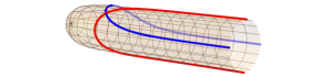
Figure 1: The D1-brane configurations in the undeformed cigar manifold embedded in $\mathbb{R}^{3}$. Heuristically, one can think of the deformation as to convert the $U(1)_{\theta}$ circle into an ellipse. However, visualising this exactly is surprisingly challenging.

Let us consider the D1-branes found above also from the semi-classical perspective. If we let $y$ be the spatial coordinate of the D1-brane and introduce $u=|\zeta|=\sinh(\rho)$ then the DBI action reads,

$$S_{DBI}=T_{1}\int\mathrm{d}y\,e^{-\Phi}\sqrt{{\rm det}\hat{G}},$$ (72)

where,

$$e^{-2\Phi}{\rm det}\hat{G} \propto u^{\prime}(y)^{2}\left(1+\lambda^{2}+2\lambda\cos(2\theta(y))\right)-4\lambda u(y)u^{\prime}(y)\theta^{\prime}(y)\sin(2\theta(y))$$ (73)

$$\qquad+u(y)^{2}\theta^{\prime}(y)^{2}\left(1+\lambda^{2}-2\lambda\cos(2\theta(y))\right).$$

Although the action evidently depends on the deformation parameter, this drops out in the classical Euler-Lagrange equations, which have a solution,

$$u(y)=\upsilon\csc(\theta_{0}+\theta(y)),$$ (74)

with $\upsilon,\theta_{0}$ integration constants. Hence, the D1-branes are semi-infinite with $u\in(\upsilon,\infty)$. Plugging this solution back into the DBI action yields,

$$S_{DBI}\propto\lim_{u\to\infty}\sqrt{u^{2}-\upsilon^{2}}\sqrt{1+\lambda^{2}+2\lambda\cos(2\theta_{0})}\ .$$ (75)

Whilst this is clearly diverging, for any UV cut-off the action is minimised by $\theta_{0}=\frac{\pi}{2},\frac{3\pi}{2}$. Asymptotically as $\rho\to\infty$ these special configurations match precisely to the integrable D-branes described in (70).

As is the case in the undeformed cigar we anticipate here also $D0$-branes localised at the tip. The corresponding worldsheet boundary conditions read,

$$\partial_{\tau}\theta=\partial_{\tau}\rho=0\ ,\quad\rho=0\ .$$ (76)

To ascertain if these constitute integrable boundary conditions we shall reverse the logic compared to the $D1$ case described above; we shall start with these boundary conditions on the field and from this infer a boundary condition on the Lax connection. A first step is to use the gauge field equations eq. (62) of motion evaluated with the gauge fixing choice eq. (61). Then the D0 boundary condition reads simply,

$$A^{1}_{+}=A^{1}_{-}\ ,\quad A^{2}_{+}=-A^{2}_{-},\quad A^{3}_{+}=A^{3}_{-}=0\ ,$$ (77)

where the latter equality follows on $\rho=0$. In terms of the Lax connection (21),

$${\cal L}_{\tau}(z)=\frac{1}{\sqrt{2\lambda}z}\left(\begin{array}[]{cc}-(1+z^{2})A_{+}^{1}&(1-z^{2})A_{+}^{2}\\ (1-z^{2})A_{+}^{2}&(1+z^{2})A_{+}^{1}\\ \end{array}\right)$$ (78)

we find that this satisfies the condition $\left.{\cal L}_{\tau}(z)\right|=\left.{\cal W}[{\cal L}_{\tau}(z^{-1})]\right|$ of (42) when ${\cal W}=\textrm{diag}(1,-1,-1)$. In this case ${\cal W}$ satisfies all necessary requirements when $\rho=0$ (since then $A_{\tau}^{3}=0$): it is a constant metric-preserving automorphism of $\mathfrak{sl}(2,R)$ and ${\cal W}^{2}(\mathfrak{g}^{(1)})=\mathbf{1}$.

In Fotopoulos:2003vc ; Ribault:2003ss it was shown that there is also a D2-brane configuration supported by a worldvolume gauge field ${\cal A}$ with field strength $F_{\rho\theta}\equiv f=\partial_{\rho}{\cal A}_{\theta}$ (in which the gauge ${\cal A}_{\rho}=0$ is adopted). In the deformed scenario we might again anticipate finding such a configuration. Indeed from the DBI action,

$$S_{DBI}\propto\int d\rho d\sigma e^{-\Phi}\sqrt{{\rm det}(G+F)},$$ (79)

we find that the $\lambda$-dependence drops from the equation of motion for the gauge field which is solved with,

$$f^{2}=\frac{\beta^{2}\tanh^{2}\rho}{-\beta^{2}+\cosh^{2}\rho}\ .$$ (80)

Here we see that when the constant $\beta>1$, the field strength $f$ is critical outside the region $\cosh\rho\geq\beta$ so that the D2-brane extends from the asymptotic circle to a minimum value in $\rho$ given by $\cosh\rho_{\star}=\beta$. When $\beta<1$, however, the D2 is space-filling.
The question now comes if this corresponds to an integrable boundary condition. Recall that a volume-filling brane should consist of generalised Neumann type boundary conditions that incorporate the gauge field $F$:

$$G_{ab}\partial_{\sigma}X^{a}=F_{ab}\partial_{\tau}X^{b}\ .$$ (81)

In terms of the coordinates $X=(\rho,\theta)$ these are quite inelegant and have explicit dependance on $\lambda$. However, we may recast this result in terms of the gauge fields $A^{(1)}_{\pm}$ using the on-shell equations of motion (62). We find that upon doing so the $\lambda$-dependence is again removed and yields,

$$(1+f^{2}\coth^{2}\rho)\{A^{1}_{-},A^{2}_{-}\}=(1-f^{2}\coth^{2}\rho)\{-A^{1}_{+},A^{2}_{+}\}-2f\coth\rho\{A^{2}_{+},A^{1}_{+}\}.$$ (82)

This tells us the gluing between the gauge fields should be field-dependent and therefore hints towards a boundary condition of the form (45) where one includes a gauge transformation in the boundary monodromy matrix. Indeed, after a tedious but straightforward computation we find that gauge transforming the Lax (21),

$${\cal L}(z)\rightarrow h^{-1}{\cal L}(z)h+h^{-1}\mathrm{d}h,$$ (83)

by,

$$h=\exp\left(v(\rho,\beta)T_{3}\right)\in H,\qquad v(\rho,\beta)=\sqrt{2}\arcsin\left(\coth^{2}\rho f^{2}+1\right)^{-1/2},$$ (84)

the integrable boundary condition (45) agrees with the D2 boundary conditions (82) when $\mathcal{W}=\text{diag}(1,-1,-1)$.

Concluding, we see here integrable D-branes corresponding to D0-, D1- and D2-configurations which are all obtained differently from a boundary condition on the Lax connection. We see also that not all of the D1-branes of the undeformed theory preserve integrability: instead of having the continuous $U(1)_{\theta}$ isometry, only two configurations at specific angles survive the integrable deformation.

3.4 Connection to Sine-Liouville theory

We are now in a position to discuss the deformation to the dual Sine-Liouville (SL) background, which in the undeformed case has the action (see for instance Kazakov:2000pm ; Fateev:2017mug ),

$$S_{SL,k}(x,\phi)=\frac{1}{\pi}\int_{\Sigma}d\tau d\sigma\;\partial_{+}\phi\partial_{-}\phi+\partial_{+}x\partial_{-}x+QR^{(2)}\phi+\mu e^{b\phi}\cos(R\tilde{x}),$$ (85)

with $R^{(2)}$ the worldsheet Ricci scalar. The target space has the topology of cylinder with $\phi\in(-\infty,+\infty)$ the radial coordinate and $x$ a $2\pi$ periodic coordinate with radius $R$ and a dual $\tilde{x}$. The parameters $Q$, $b$ and $R$ are related as $Q=-1/b$ and $R^{2}-b^{2}=2$ ensuring Sine-Liouville is an exact CFT with central charge,

$$c=2+6Q^{2},$$ (86)

and a potential $V(\phi,\tilde{x})=\mu e^{b\phi}\cos(R\tilde{x})$ with scaling dimension $1$. The central charge of the Euclidean cigar (51) matches with that of SL when $Q^{2}=\frac{1}{k-2}$, hence (taking the positive root of $Q$) we have $b=-\sqrt{k-2}$ and $R=\sqrt{k}$.
A dictionary between the (undeformed) Euclidean cigar black hole and Sine-Liouville theory can be made in the asymptotic flat space limit $\rho\rightarrow\infty$ where the cigar approaches the toplogy of a cylinder and its dilaton falls off linearly, $\Phi_{A}-\Phi_{0}\rightarrow-\rho$. On the SL side, this limit corresponds to the region $\phi\rightarrow\infty$ in which the potential $V(\phi,\tilde{x})$ as well as the string coupling constant go to zero given the dilaton $\Phi_{SL}=Q\phi$. The identification is therefore at large $k$ given by,

$$\rho\sim-Q\phi,\qquad\theta\sim\frac{x}{\sqrt{k}},\qquad\tilde{\chi}\sim\sqrt{k}\tilde{x}\ .$$ (87)

At finite $\rho$ and $\phi$, the duality between both theories can be demonstrated as an exact match between the symmetry algebra’s, vertex operators and $n$-point functions Fateev:SL ; Kazakov:2000pm ; Hikida:2008pe (see also Fateev:2017mug ) where they look both topologically and dynamically very different. Indeed, it can be understood that the dynamics is governed by the geometry in the cigar picture and by the potential $V(\phi,\tilde{x})$ in the SL picture. Additionally, the tip of the cigar is the end of space corresponding to the horizon of the Euclidean black hole and hence cutting off the strong string coupling region, while on the SL side this region is protected by the potential $V(\phi,\tilde{x})$. On the worldsheet the duality can be viewed as a strong-weak coupling duality. However, the sigma model point of view taken here forces us in the small coupling (large $k$) regime on the cigar side.
For us the power of the duality lies in the observation that the semi-classical cigar parafermions (54) in the flat space limit under the identification (87),

$$\Psi_{(\pm)}^{SL} =\left(-\frac{\partial_{+}\phi}{\sqrt{k-2}}\mp i\frac{\partial_{+}x}{\sqrt{k}}\right)e^{\mp\frac{2ix_{L}}{\sqrt{k}}},\qquad\bar{\Psi}_{(\pm)}^{SL}=\left(-\frac{\partial_{-}\phi}{\sqrt{k-2}}\pm i\frac{\partial_{-}x}{\sqrt{k}}\right)e^{\pm\frac{2ix_{R}}{\sqrt{k}}},$$ (88)

commute with the SL potential $V(\phi,\tilde{x})$ Fateev:2017mug . Here $x(\sigma^{+},\sigma^{-})=x_{L}(\sigma^{+})+x_{R}(\sigma^{-})$ and $\tilde{x}(\sigma^{+},\sigma^{-})=x_{L}(\sigma^{+})-x_{R}(\sigma^{-})$. Therefore, one can rely on the expression (88) for all values of $\phi$. Since the parafermion fields induce the deformation (66) we can now easily extract the perturbation on the SL theory side. To first order in $\lambda$ the deforming term in the large $k$ regime becomes,

$$\delta L_{SL}=\lambda \left(2\cos\left(\frac{2x}{R}\right)\partial_{+}\phi\partial_{-}\phi-2\cos\left(\frac{2x}{R}\right)\partial_{+}x\partial_{-}x\right.$$ (89)

$$\;\;\left.+2\sin\left(\frac{2x}{R}\right)(\partial_{+}x\partial_{-}\phi+\partial_{-}x\partial_{+}\phi)\right)+{\cal O}(\lambda^{2})\ .$$

A similar structure is expected for finite $\lambda$, as (66) is exact in $\lambda$, so that one deforms the flat space SL theory to a curved background. We anticipate this is the starting point of an integrable deformation of the SL theory. Moreover, it appears to be in a different class to the integrable deformations studied in Fateev:2017mug . We will leave this as an open problem to be fully understood.

4 Conclusion

The Sfetsos procedure Sfetsos:2013wia to construct the $\lambda$-deformation of a $G/H$ coset realised as a gauged WZW model actually requires the $G/G$ model as a starting point. To date, even when $H$ is abelian, attention has been restricted to the case in which in the $G/G$ model the $G$ symmetry, and consequently that of $H$, acts vectorially. Here we explore the asymmetric gauging of $G$ in which the left and right actions differ by the application of an algebra automorphism. When this is an outer automorphism what results can not be trivially removed via field redefinitions. In this way, we are able to produce new $\lambda$-type deformations leading to topologically distinct target spaces in a robust and fundamental manner. Using the similarities between this asymmetric $\lambda$-model and its vectorial cousin we demonstrate classical integrability and show the one-loop beta functions to stay marginally relevant for compact groups and irrelevant for non-compact groups. To end our general discussion of this model, we present a simple technique to construct integrable boundary conditions in which we, moreover, exploit the residual asymmetric gauge symmetry.
As an example we consider the $SL(2,R)/U(1)$ model where unlike the compact $SU(2)$ there is such a non-trivial outer automorphism. We show that employing our procedure we are able to find an integrable deformation of the theory in which the gauged symmetry acts axially. Geometrically, and at large $k$, we have an integrable deformation of the cigar geometry corresponding to the Euclideanised Witten black hole. The cigar geometry itself receives $\frac{1}{k}$ corrections and it would be doubtless valuable to find a description of the $\lambda$-deformation that takes these corrections into account. Continuing at large $k$, we analyse also the boundary conditions preserving integrability in the deformed cigar. We see this can be done straightforwardly and observe the D-branes proposed at the (non-rational) CFT point to be integrable in the deformation.

As well as demonstrating the concept for this broader class of deformations we believe this example could hold some further interest in its own right. Let us entertain some speculation about how the deformation translates to both the Sine-Liouville (SL) dual and in turn to the matrix model description of this picture. An initial step is made here by identifying for small deformation parameters in the cigar a bilinear of the non-compact parafermions as the operators that drive the deformation. Demanding agreement between the SL at large values of the radial coordinate suggests strongly the same parafermionic bilinear deformation should be considered in the SL model. However the $\lambda$-model goes much further since it provides a resummation to all orders in $\lambda$ of this deformation; what this looks like in the SL theory is far from clear. One possible root to shed light on this could be to combine the Sfetsos procedure with the path integral derivation of FZZ. When successful, one can continue and probe, using the deformed SL theory and integrability, the region behind the horizon.
It is also interesting to ask what the deformation does at the level of the S-matrix. For the case of similar deformations of compact parafermionic theories it has long been known that the S-matrix has a kink structure and in the $k\to\infty$ limit matches that of the $O(3)$ sigma-model Fateev:1991bv . A similar expectation holds for general $\lambda$-deformations, the underlying S-matrix has a $q$ root-of-unity quantum group symmetry associated to a face model Hollowood:2015dpa ; Appadu:2017fff . Here it is less clear due to the non-compactness of the theory but one might well anticipate a similar $q$-deformation to hold. Further one might ask what this structure might relate to in the postulated dual matrix model description of the cigar Kazakov:2000pm .
A final enticing direction is to employ similar techniques in the context of geometries relevant to black hole microstates. For instance a static configuration of NS5-branes on a circle admits a description as a gauged WZW model Sfetsos:1998xd ; Israel:2004ir , and more general solutions (supertubes and spectral flows of supertubes) can also be realised as gauged WZW models Martinec:2017ztd ; Martinec:2018nco . It seems quite possible that the techniques developed here may be applicable to such situations. We leave that for future work.

Appendix A Conventions and sigma models (WZW, PCM and SSSM)

In this appendix, we briefly introduce some basic ingredients and conventions for the gauging procedure of section 2.

For the general formulae of this paper we adopt conventions for compact and semi-simple groups $G$, although they should be changed conveniently when working out the non-compact $SL(2,R)/U(1)$ example in section 3. We denote the generators of the Lie algebra $\mathfrak{g}$ of $G$ by $T_{A}$ and pick a basis in which they are Hermitean, i.e. $\left[T_{A},T_{B}\right]=iF_{AB}{}^{C}T_{C}$ with real structure constants $F_{AB}{}^{C}$ and $A=\{1,\cdots,\dim G\}$. They are normalised in such a way that the ad-invariant Cartan-Killing metric $\langle\cdot,\cdot\rangle:\mathfrak{g}\times\mathfrak{g}\rightarrow\mathbb{R}$, taken to be $\langle T_{A},T_{B}\rangle=\frac{1}{x_{R}}\operatorname{Tr}\left(T_{A}T_{B}\right)$ with $x_{R}$ the index of the representation $R$, has unit entries. The left-(right-)invariant Maurer-Cartan one-forms are expanded in the Lie algebra as $g^{-1}\mathrm{d}g=-iL^{A}T_{A}$ ($\mathrm{d}gg^{-1}=-iR^{A}T_{A}$) and in explicit local coordinates $X^{\mu}$, $\mu\in\{1,\cdots,\dim G\}$ as $g^{-1}\mathrm{d}g=-iL^{A}{}_{\mu}(X)T_{A}\mathrm{d}X^{\mu}$ ($\mathrm{d}gg^{-1}=-iR^{A}{}_{\mu}(X)T_{A}\mathrm{d}X^{\mu}$). The adjoint action is denoted by $D_{g}T_{A}=gT_{A}g^{-1}=(D_{g})^{B}{}_{A}T_{B}$, hence $(D_{g})_{AB}=\langle T_{A},gT_{B}g^{-1}\rangle$ and $R^{A}=(D_{g})^{A}{}_{B}L^{B}$.
Finally, considering the $G/H$ coset, we denote the generators of the subgroup $H\subset G$ with Lie algebra $\mathfrak{h}$ by $T_{a}$, $a=\{1,\cdots,\text{dim}H\}$ and the remaining generators by $T_{\alpha}$, $\alpha=\{\text{dim}H+1,\cdots,\text{dim}G\}$. We assume the Lie algebra $\mathfrak{g}$ to have a symmetric space decomposition $\mathfrak{g}=\mathfrak{g}^{(0)}\oplus\mathfrak{g}^{(1)}$, with $\mathfrak{g}^{(0)}\equiv\mathfrak{h}$, defined by a $\mathbb{Z}_{2}$ grading $[\mathfrak{g}^{(i)},\mathfrak{g}^{(j)}]\subset\mathfrak{g}^{(i+j\text{ mod }2)}$.

We consider the WZW model on a Lie group manifold $G$ at level $k$ Witten:1983ar with the action,

$$S_{\mbox{\tiny{WZW}},k}(g)=-\frac{k}{2\pi}\int_{\Sigma}d\sigma d\tau\langle g^{-1}\partial_{+}g,g^{-1}\partial_{-}g\rangle-\frac{k}{24\pi}\int_{M_{3}}\langle\bar{g}^{-1}\mathrm{d}\bar{g},\left[\bar{g}^{-1}\mathrm{d}\bar{g},\bar{g}^{-1}\mathrm{d}\bar{g}\right]\rangle,$$ (90)

with $g:\Sigma\rightarrow G$ a Lie group element and $\bar{g}$ an extension of $g$ into $M_{3}\subset G$ such that $\partial M_{3}=g(\Sigma)$. To cancel ambiguities from the choice of $M_{3}$ in the path integral the level $k$ should be integer quantised for compact groups while for non-compact cases it can be free Witten:1983ar ; Figueroa-OFarrill:2000lcd . The two-dimensional manifold $\Sigma$ can be thought of as a worldsheet on which we have fixed the metric as $\text{diag}(+1,-1)$, the Levi-Civita as $\epsilon_{\tau\sigma}=1$ and we have units in which $\alpha^{\prime}=1$ . We analytically continue to Euclidean coordinates by taking $\sigma_{+}=\tau+\sigma\to-iz$ and $\sigma_{-}=\tau-\sigma\to-i\bar{z}$ and will use the term holomorphic abusively to mean either $f(\sigma^{+})$ or $f(z)$. The WZW model on group manifolds is known to have an exact CFT formulation originating from the $G_{L}(\sigma^{+})\times G_{R}(\sigma^{-})$ symmetry generated by the holomorphically conserved currents $J_{+}(\sigma^{+})=-k\partial_{+}gg^{-1}$ and $J_{-}(\sigma^{-})=kg^{-1}\partial_{-}g$ whose components satisfy two commuting Kac-Moody algebra’s.
We consider moreover the PCM model on a Lie group manifold $G$ with a coupling constant $\kappa^{2}$,

$$S_{\mbox{\tiny{PCM}},\kappa^{2}}(\widehat{g})=-\frac{\kappa^{2}}{\pi}\int d\sigma d\tau\langle\widehat{g}^{-1}\partial_{+}\widehat{g},\widehat{g}^{-1}\partial_{-}\widehat{g}\rangle,\quad\widehat{g}\in G,$$ (91)

which has a global $G_{L}\times G_{R}$ symmetry. From the PCM model the SSSM model on the $G/H$ coset manifold can be obtained by gauging an $H_{R}\subset G$ subgroup acting as,

$$\widehat{g}\rightarrow\widehat{g}h.$$ (92)

The gauge-invariant action is then,

$$S_{\mbox{\tiny{SSSM}},\kappa^{2}}(\widehat{g},B_{\pm})=-\frac{\kappa^{2}}{\pi}\int d\sigma d\tau\langle(\widehat{g}^{-1}\partial_{+}\widehat{g}-B_{+}),(\widehat{g}^{-1}\partial_{-}\widehat{g}-B_{-})\rangle,$$ (93)

with $B_{\pm}$ the gauge fields taking values in the Lie algebra $\mathfrak{g}^{(0)}\equiv\mathfrak{h}$ of $H$ and transforming under the gauge transformation as $B_{\pm}\rightarrow h^{-1}\left(B_{\pm}+\partial_{\pm}\right)h$. This model is easily shown to be classically integrable when $\mathfrak{g}=\mathfrak{g}^{(0)}\oplus\mathfrak{g}^{(1)}$ has a symmetric space decomposition Eichenherr:1979ci ; Hollowood:2014rla .

Note that when working with non-compact groups, where one picks an anti-Hermitean basis to have real structure constants, one should analytically continue in the above models $k\rightarrow-k$ and $\kappa^{2}\rightarrow-\kappa^{2}$ in order to keep the right sign on the kinetic term.

References

- (1) I. Bena, J. Polchinski and R. Roiban, Hidden symmetries of the AdS(5) x S**5 superstring, Phys. Rev. D69 (2004) 046002 [hep-th/0305116].
- (2) N. Beisert et al., Review of AdS/CFT Integrability: An Overview, Lett. Math. Phys. 99 (2012) 3 [1012.3982].
- (3) G. Arutyunov and S. Frolov, Foundations of the Superstring. Part I, J. Phys. A42 (2009) 254003 [0901.4937].
- (4) E. Witten, Nonabelian Bosonization in Two-Dimensions, Commun. Math. Phys. 92 (1984) 455.
- (5) A. M. Polyakov, Interaction of Goldstone Particles in Two-Dimensions. Applications to Ferromagnets and Massive Yang-Mills Fields, Phys. Lett. 59B (1975) 79.
- (6) K. Gawedzki and A. Kupiainen, G/h Conformal Field Theory from Gauged WZW Model, Phys. Lett. B215 (1988) 119.
- (7) D. Karabali, Q.-H. Park, H. J. Schnitzer and Z. Yang, A GKO Construction Based on a Path Integral Formulation of Gauged Wess-Zumino-Witten Actions, Phys. Lett. B216 (1989) 307.
- (8) H. Eichenherr and M. Forger, On the Dual Symmetry of the Nonlinear Sigma Models, Nucl. Phys. B155 (1979) 381.
- (9) O. Lunin and J. M. Maldacena, Deforming field theories with U(1) x U(1) global symmetry and their gravity duals, JHEP 05 (2005) 033 [hep-th/0502086].
- (10) C. Klimcik, On integrability of the Yang-Baxter sigma-model, J. Math. Phys. 50 (2009) 043508 [0802.3518].
- (11) F. Delduc, M. Magro and B. Vicedo, On classical -deformations of integrable sigma-models, JHEP 11 (2013) 192 [1308.3581].
- (12) F. Delduc, M. Magro and B. Vicedo, An integrable deformation of the superstring action, Phys. Rev. Lett. 112 (2014) 051601 [1309.5850].
- (13) I. Kawaguchi, T. Matsumoto and K. Yoshida, Jordanian deformations of the superstring, JHEP 04 (2014) 153 [1401.4855].
- (14) D. Osten and S. J. van Tongeren, Abelian Yang–Baxter deformations and TsT transformations, Nucl. Phys. B915 (2017) 184 [1608.08504].
- (15) R. Borsato and L. Wulff, Marginal deformations of WZW models and the classical Yang-Baxter equation, 1812.07287.
- (16) K. Sfetsos, Integrable interpolations: From exact CFTs to non-Abelian T-duals, Nucl. Phys. B880 (2014) 225 [1312.4560].
- (17) T. J. Hollowood, J. L. Miramontes and D. M. Schmidtt, Integrable Deformations of Strings on Symmetric Spaces, JHEP 11 (2014) 009 [1407.2840].
- (18) T. J. Hollowood, J. L. Miramontes and D. M. Schmidtt, An Integrable Deformation of the Superstring, J. Phys. A47 (2014) 495402 [1409.1538].
- (19) C. Appadu and T. J. Hollowood, Beta function of k deformed AdS5 x S5 string theory, JHEP 11 (2015) 095 [1507.05420].
- (20) R. Borsato, A. A. Tseytlin and L. Wulff, Supergravity background of -deformed model for AdS S2 supercoset, Nucl. Phys. B905 (2016) 264 [1601.08192].
- (21) Y. Chervonyi and O. Lunin, Supergravity background of the -deformed AdS S3 supercoset, Nucl. Phys. B910 (2016) 685 [1606.00394].
- (22) R. Borsato and L. Wulff, Target space supergeometry of and -deformed strings, JHEP 10 (2016) 045 [1608.03570].
- (23) K. Sfetsos and D. C. Thompson, Spacetimes for -deformations, JHEP 12 (2014) 164 [1410.1886].
- (24) S. Demulder, K. Sfetsos and D. C. Thompson, Integrable -deformations: Squashing Coset CFTs and , JHEP 07 (2015) 019 [1504.02781].
- (25) E. Witten, On Holomorphic factorization of WZW and coset models, Commun. Math. Phys. 144 (1992) 189.
- (26) P. H. Ginsparg and F. Quevedo, Strings on curved space-times: Black holes, torsion, and duality, Nucl. Phys. B385 (1992) 527 [hep-th/9202092].
- (27) I. Bars and K. Sfetsos, Generalized duality and singular strings in higher dimensions, Mod. Phys. Lett. A7 (1992) 1091 [hep-th/9110054].
- (28) G. Georgiou, K. Sfetsos and K. Siampos, -Deformations of left–right asymmetric CFTs, Nucl. Phys. B914 (2017) 623 [1610.05314].
- (29) G. Georgiou and K. Sfetsos, A new class of integrable deformations of CFTs, JHEP 03 (2017) 083 [1612.05012].
- (30) G. Georgiou and K. Sfetsos, The most general -deformation of CFTs and integrability, 1812.04033.
- (31) E. Witten, On string theory and black holes, Phys. Rev. D44 (1991) 314.
- (32) S. Elitzur, A. Forge and E. Rabinovici, Some global aspects of string compactifications, Nucl. Phys. B359 (1991) 581.
- (33) G. Mandal, A. M. Sengupta and S. R. Wadia, Classical solutions of two-dimensional string theory, Mod. Phys. Lett. A6 (1991) 1685.
- (34) M. Rocek, K. Schoutens and A. Sevrin, Off-shell WZW models in extended superspace, Phys. Lett. B265 (1991) 303.
- (35) A. A. Tseytlin, Effective action of gauged WZW model and exact string solutions, Nucl. Phys. B399 (1993) 601 [hep-th/9301015].
- (36) I. Bars and K. Sfetsos, Exact effective action and space-time geometry n gauged WZW models, Phys. Rev. D48 (1993) 844 [hep-th/9301047].
- (37) R. Dijkgraaf, H. L. Verlinde and E. P. Verlinde, String propagation in a black hole geometry, Nucl. Phys. B371 (1992) 269.
- (38) A. Giveon, Target space duality and stringy black holes, Mod. Phys. Lett. A6 (1991) 2843.
- (39) E. B. Kiritsis, Duality in gauged WZW models, Mod. Phys. Lett. A6 (1991) 2871.
- (40) M. Rocek and E. P. Verlinde, Duality, quotients, and currents, Nucl. Phys. B373 (1992) 630 [hep-th/9110053].
- (41) V. Kazakov, I. K. Kostov and D. Kutasov, A Matrix model for the two-dimensional black hole, Nucl. Phys. B622 (2002) 141 [hep-th/0101011].
- (42) V. A. Fateev, A. B. Zamolodchikov and A. B. Zamolodchikov, “unpublished.”.
- (43) Y. Hikida and V. Schomerus, The FZZ-Duality Conjecture: A Proof, JHEP 03 (2009) 095 [0805.3931].
- (44) A. Giveon, N. Itzhaki and D. Kutasov, Stringy Horizons, JHEP 06 (2015) 064 [1502.03633].
- (45) S. Driezen, A. Sevrin and D. C. Thompson, D-branes in -deformations, JHEP 09 (2018) 015 [1806.10712].
- (46) A. Fotopoulos, Semiclassical description of D branes in SL(2) / U(1) gauged WZW model, Class. Quant. Grav. 20 (2003) S465 [hep-th/0304015].
- (47) S. Ribault and V. Schomerus, Branes in the 2-D black hole, JHEP 02 (2004) 019 [hep-th/0310024].
- (48) A. Fotopoulos, V. Niarchos and N. Prezas, D-branes and extended characters in SL(2,R) / U(1), Nucl. Phys. B710 (2005) 309 [hep-th/0406017].
- (49) D. Israel, A. Pakman and J. Troost, D-branes in N=2 Liouville theory and its mirror, Nucl. Phys. B710 (2005) 529 [hep-th/0405259].
- (50) S. Ribault, Discrete D-branes in AdS(3) and in the 2-D black hole, JHEP 08 (2006) 015 [hep-th/0512238].
- (51) J. M. Maldacena, G. W. Moore and N. Seiberg, Geometrical interpretation of D-branes in gauged WZW models, JHEP 07 (2001) 046 [hep-th/0105038].
- (52) A. M. Polyakov and P. B. Wiegmann, Goldstone Fields in Two-Dimensions with Multivalued Actions, Phys. Lett. 141B (1984) 223.
- (53) P. Bowcock, Canonical Quantization of the Gauged Wess-Zumino Model, Nucl. Phys. B316 (1989) 80.
- (54) K. Sfetsos, K. Siampos and D. C. Thompson, Generalised integrable - and -deformations and their relation, Nucl. Phys. B899 (2015) 489 [1506.05784].
- (55) V. E. Zakharov and A. V. Mikhailov, Relativistically Invariant Two-Dimensional Models in Field Theory Integrable by the Inverse Problem Technique. (In Russian), Sov. Phys. JETP 47 (1978) 1017.
- (56) G. Itsios, K. Sfetsos and K. Siampos, The all-loop non-Abelian Thirring model and its RG flow, Phys. Lett. B733 (2014) 265 [1404.3748].
- (57) K. Sfetsos and K. Siampos, Gauged WZW-type theories and the all-loop anisotropic non-Abelian Thirring model, Nucl. Phys. B885 (2014) 583 [1405.7803].
- (58) I. V. Cherednik, Factorizing Particles on a Half Line and Root Systems, Theor. Math. Phys. 61 (1984) 977.
- (59) E. K. Sklyanin, Boundary Conditions for Integrable Quantum Systems, J. Phys. A21 (1988) 2375.
- (60) A. Dekel and Y. Oz, Integrability of Green-Schwarz Sigma Models with Boundaries, JHEP 08 (2011) 004 [1106.3446].
- (61) O. Babelon, D. Bernard and M. Talon, Introduction to Classical Integrable Systems, Cambridge Monographs on Mathematical Physics. Cambridge University Press, 2003, 10.1017/CBO9780511535024.
- (62) J. D. Lykken, Finitely Reducible Realizations of the Superconformal Algebra, Nucl. Phys. B313 (1989) 473.
- (63) I. Bakas and E. Kiritsis, Beyond the large N limit: Nonlinear W(infinity) as symmetry of the SL(2,R) / U(1) coset model, Int. J. Mod. Phys. A7S1A (1992) 55 [hep-th/9109029].
- (64) V. A. Fateev and A. B. Zamolodchikov, Parafermionic Currents in the Two-Dimensional Conformal Quantum Field Theory and Selfdual Critical Points in Z(n) Invariant Statistical Systems, Sov. Phys. JETP 62 (1985) 215.
- (65) D. Israel, C. Kounnas and M. P. Petropoulos, Superstrings on NS5 backgrounds, deformed AdS(3) and holography, JHEP 10 (2003) 028 [hep-th/0306053].
- (66) K. Bardakci, M. J. Crescimanno and E. Rabinovici, Parafermions From Coset Models, Nucl. Phys. B344 (1990) 344.
- (67) P. Marios Petropoulos and K. Sfetsos, NS5-branes on an ellipsis and novel marginal deformations with parafermions, JHEP 01 (2006) 167 [hep-th/0512251].
- (68) T. H. Buscher, A Symmetry of the String Background Field Equations, Phys. Lett. B194 (1987) 59.
- (69) T. H. Buscher, Path Integral Derivation of Quantum Duality in Nonlinear Sigma Models, Phys. Lett. B201 (1988) 466.
- (70) E. Alvarez, L. Alvarez-Gaume and Y. Lozano, A Canonical approach to duality transformations, Phys. Lett. B336 (1994) 183 [hep-th/9406206].
- (71) V. A. Fateev and A. B. Zamolodchikov, Integrable perturbations of Z(N) parafermion models and O(3) sigma model, Phys. Lett. B271 (1991) 91.
- (72) C. Bachas and M. Petropoulos, Anti-de Sitter D-branes, JHEP 02 (2001) 025 [hep-th/0012234].
- (73) T. Quella and V. Schomerus, Symmetry breaking boundary states and defect lines, JHEP 06 (2002) 028 [hep-th/0203161].
- (74) V. A. Fateev, Integrable Deformations of Sine-Liouville Conformal Field Theory and Duality, SIGMA 13 (2017) 080 [1705.06424].
- (75) T. J. Hollowood, J. L. Miramontes and D. M. Schmidtt, S-Matrices and Quantum Group Symmetry of k-Deformed Sigma Models, J. Phys. A49 (2016) 465201 [1506.06601].
- (76) C. Appadu, T. J. Hollowood and D. Price, Quantum Inverse Scattering and the Lambda Deformed Principal Chiral Model, J. Phys. A50 (2017) 305401 [1703.06699].
- (77) K. Sfetsos, Branes for Higgs phases and exact conformal field theories, JHEP 01 (1999) 015 [hep-th/9811167].
- (78) D. Israel, C. Kounnas, A. Pakman and J. Troost, The Partition function of the supersymmetric two-dimensional black hole and little string theory, JHEP 06 (2004) 033 [hep-th/0403237].
- (79) E. J. Martinec and S. Massai, String Theory of Supertubes, JHEP 07 (2018) 163 [1705.10844].
- (80) E. J. Martinec, S. Massai and D. Turton, String dynamics in NS5-F1-P geometries, JHEP 09 (2018) 031 [1803.08505].
- (81) J. M. Figueroa-O’Farrill and S. Stanciu, D-brane charge, flux quantization and relative (co)homology, JHEP 01 (2001) 006 [hep-th/0008038].