CPOI: A Compact Method to Archive
Versioned RDF Triple-Sets

Abstract

Large amounts of RDF/S data are produced and published lately, and several modern applications require the provision of versioning and archiving services over such datasets. In this paper we propose a novel storage index for archiving versions of such datasets, called CPOI (compact partial order index), that exploits the fact that an RDF Knowledge Base (KB), is a graph (or equivalently a set of triples), and thus it has not a unique serialization (as it happens with text). If we want to keep stored several versions we actually want to store multiple sets of triples. CPOI is a data structure for storing such sets aiming at reducing the storage space since this is important not only for reducing storage costs, but also for reducing the various communication costs and enabling hosting in main memory (and thus processing efficiently) large quantities of data. CPOI is based on a partial order structure over sets of triple identifiers, where the triple identifiers are represented in a gapped form using variable length encoding schemes. For this index we evaluate analytically and experimentally various identifier assignment techniques and their space savings. The results show significant storage savings, specifically, the storage space of the compressed sets in large and realistic synthetic datasets is about the 8% of the size of the uncompressed sets.

1 Introduction

The rising tide of data is a main characteristic of our age: “We create as much information in two days now as we did from the dawn of man through 2003”. A large proportion of these data are scientific. For instance, and according to [10], the first “reading” of the human genome created digital records on more than 250 billion DNA bases in less than 10 years, while the evolution of European Space Agency’s Earth Observation data archives passed three petabytes in 2007 (the projection for 2020 is a seven-fold rise). For scientific data the provision of versioning services is important for various purposes (archiving, preservation, provenance). For instance, failure to keep the previous states of scientific data (over which other experiments were based) jeopardizes scientific evidence and our ability to verify findings [3].

Lately, an increasing amount of data (including scientific data) is published on the Web in RDF/S according to the Linked Open Data (LOD) principles [2] and various applications, e.g. in life sciences [9, 6], require the provision of versioning services over RDF datasets (either schema-free or schema-based). It follows that versioning services over large amounts of structured (scientific) data is a requirement from which we cannot escape.

Two key performance aspects of a version management system is the storage space and the time for creating (resp. retrieving) a new (resp. existing) version. Most of the related works in the SW (Semantic Web) focus on high level functions and they mainly overlook the storage space perspective which is fundamental. It should be stressed that the space perspective is important not only for (a) reducing storage costs, but also for (b) reducing the various communication costs (e.g. loading times from disk or across networks), and (c) enabling hosting in main memory (and thus processing efficiently) large quantities of data.

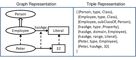
Figure 1: An RDF KB as a graph and the corresponding set of triples

An RDF/S KB (Knowledge Base) can be viewed as a graph or as a set of triples, as illustrated in the example of Figure 1. Regarding storage, we can identify the following main approaches of a versions management system.
(a) Independent Copies (IC): Every version is stored independently and this policy is adopted in [22, 16, 12].
(b) Change Based (CB): Only deltas between subsequent versions are stored, a policy that is adopted in various tools for versioning software [19, 1], and it has been proposed also for Semantic Web data [24, 20].
(c) Timestamp Based (TSB): Each triple is enriched with time-stamps indicating the versions the triple belongs to ([20, 15]). Proposals like [8] fall into the same category too.

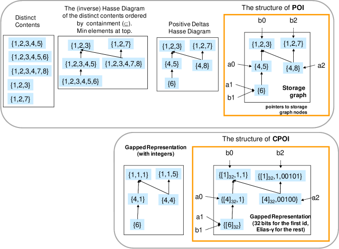
Figure 2: The structure of POI and the introduced compact representation CPOI

In [21] a storage structure, called POI  (Partial Order Index) has been proposed. POI exploits the fact that RDF KBs have not a unique serialization (as it happens with texts) and it offers notable space savings in comparison to the change-based approach, as well as efficiency in various cross version operations. POI views an RDF KB as a set of triples and exploits the expected overlap between versions’ contents in order to reduce the storage space. We shall describe POI using an example.

Example 1.1

Consider six (6) KBs, denoted by a0, a1, a2, b0, b1 and b2. Each KB consists of a set of triples and each triple is assigned a unique numeric identifier. Specifically suppose that:
a0={1, 2, 3, 4, 5} b0={1, 2, 3} a1={1, 2, 3, 4, 5, 6} b1={1, 2, 3, 4, 5, 6} a2={1, 2, 3, 4, 7, 8} b2={1, 2, 7}  
Furthermore suppose that there are two evolution tracks a0 $\rightarrow$ a1 $\rightarrow$ a2 (meaning that a1 is the next version of a0, and that a2 is the next version of a1), and b0 $\rightarrow$ b1 $\rightarrow$ b2. The upper part of Figure 2 depicts the structure of POI. The first diagram shows the set of distinct triple sets, the second diagram shows the proper subset ($\subset$) relationships that hold between these sets, while in the third diagram each node does not contain triples “inherited” from parent nodes. This is the storage graph of POI. The fourth diagram shows the entire structure for POI, where each version id points to the corresponding node of the storage graph. For instance, version a1 points to a node storing only the triple identifier 6. The full contents of a1 are obtained by taking the union of the triples stored at that node and its parent nodes, i.e. $\{6\}\cup\{4,5\}\cup\{1,2,3\}=\{1,2,3,4,5,6\}$. Finally, there is a table $TStrings$ which maps each triple id to the corresponding triple string, e.g. $2\rightarrow``(Peter,type,Employee)"$.
$\diamond$

In brief, POI stores explicitly only the triple ids of the versions with the minimal (with respect to set containment) contents. All the rest versions are stored in a positively incremental way which is history-independent. Past experiments over synthetic datasets have shown [21] that POI occupies less space than the change-based approach. Regarding version retrieval time, the cost of retrieving the contents of a version in POI is independent of any kind of history (in comparison with the change-based approach), but it depends on the contents of the particular version, specifically on the depth of the corresponding node in the POI graph.

In this paper we investigate whether techniques which have been used with success in the area of IR (Information Retrieval) systems and WSE (Web Search Engines) can be exploited for RDF data. In IR, the adoption of variable length encoding schemes in the posting lists of an inverted index offers significant space savings. Specifically, if the documents that share a lot of common words get close identifiers, and we adopt a gapped representation (explained in the continuation of the running example) for their identifiers using an encoding scheme that represents small integers with a small number of bits, then the postings lists of these common words will have small bit representation. Experiments in the IR domain (specifically in the TREC web data [18]) have shown that the compression ratio, defined as the size of the compressed file as a percentage of the uncompressed file (i.e. $Compression\ ratio=\frac{Compressed\ size}{Uncompressed\ size}100\%$), is around 30%-45%. In our case, since each triple has a unique identifier, and hence each node of POI stores a set of identifiers, we investigate whether special identifier assignments and integer encodings, such as Elias-$\gamma$ [4], can reduce (and under what conditions) the occupied space. Although POI by construction offers significant storage gains, the motivation for investigating this approach is not only for reducing the space requirements of POI in the expected application scenarios, but also for tackling the cases where there are several overlapping versions which are not related by inclusion. In such cases, POI behaves like the IC approach. It would be desirable to have an index structure that behaves well also in extreme cases. An appropriate identifier encoding promises space gains also in such cases.

Hereafter we shall use the term CPOI (Compact POI) to refer to a compact version of POI, that relies on gapped numeric identifiers and special encodings. To grasp the idea below we explain CPOI over the running example.

Example 1.1 (cont.). The lower part of Figure 2 shows the gapped representation of the nodes’s contents with integers (left), for our running example. In this representation we consider the elements of a node as a list of ids in ascending order and we keep the first id unchanged while each one of the rest ids is replaced by its difference from the previous id. The right part of that Figure shows the final form of CPOI. Specifically, the first value of every node is represented as a normal (32-bit representation) integer, while the rest values are represented using a special encoding for integers (here, Elias-$\gamma$).
$\diamond$

In this paper, apart from proposing CPOI, we compare the sizes of POI and CPOI analytically, and we identify conditions under which CPOI guarantees space savings. Since the conditions are based on bounds (i.e. they are sufficient, not necessary conditions), we also report extensive experimental results over synthetic and real datasets of various characteristics. We comparatively evaluate various identifier assignment or reassignment policies, like first-in-first-served, triple frequency, as well as policies based on the structure of storage graph of POI. The results show that in realistic synthetic datasets, the compression ratio achieved by CPOI regarding the contents of the nodes is 7.5%. The only price to pay, in comparison to the rest approaches is slower additions of new versions, however since a version is added only once, CPOI is a beneficial choice for archiving.

The remainder of this paper is structured as follows: Section 2 discusses related work. Section 3 introduces CPOI and provides lower and upper bounds for its space requirements. Section 4 proposes methods for assigning identifiers to triples. Section 5 reports extensive comparative experimental results for various datasets. Subsequently Section 6 discusses possible applications of CPOI, and finally, Section 7 summarizes and concludes the paper. Proofs and supplementary measurements are given at the appendix.

2 Related Work

We shall make clear the differences between the IC, CB and POI  approaches through an example. Figure 3 shows a set of triples and their assigned identifiers. Figure 4 illustrates what is stored according to the IC and CB approach, while Figure 5 shows what will be stored according to the POI approach.

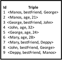
Figure 3: Triple strings and their identifiers

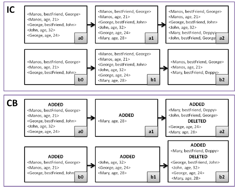
Figure 4: Storing versions according to IC and CB approach

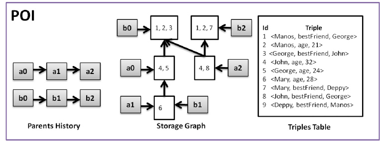
Figure 5: Storing versions according to the POI approach

Obviously, the IC approach does not offer any space savings as every version is stored independently. CB behaves well in cases like: the contents of the KBs form a chain with respect to $\subseteq$ and they are consecutive in the version history. The worst case for CB occurs when we have a track where the same set of triples is once added and once deleted in an alternative fashion. In that case CB requires more space than IC (even 2 times worse). The worst case for POI is when all nodes of the storage graph are leaves (i.e. the graph is flat), leading to space requirements equal to those of IC. On the other hand, the best case for POI, is when the content of every version is a subset of the content of every version with greater (or equal) content cardinality. In that case every triple id is stored only once in the storage graph. Fig. 6 illustrates a good and bad case for POI (this figure illustrates the various approaches only according to triple identifiers, neither triple strings nor any other data structure-related cost).

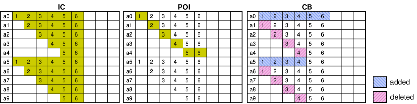
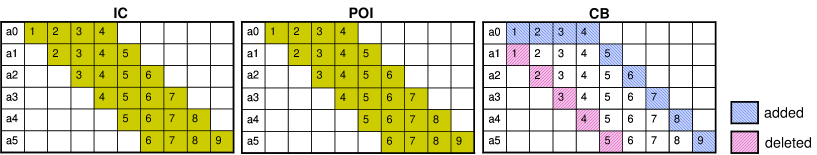
Figure 6: A good (upper) and a bad (bottom) case for POI

Also note that the best case for both CB and POI leads to the same space requirements, while this does not hold for the worst case, which is much better in the case of POI.

Regarding the TSB (timestamp) approach, each distinct triple is enriched with pairs of in/out timestamps (similar in spirit with [3] for XML). TSB is not beneficial for version sequences which do not form chains (as timestamps presuppose a linear order of versions, e.g. [11] supports only chains). The reconstruction of the contents of a version is slow in TSB as it requires looking up the timestamps of all triples, unless extra structures (with additional space costs) are adopted. The only fast task is to check whether a particular triple belongs to a version, but this is not important for our application scenario (version archiving). Instead POI offers fast reconstruction of version contents (by taking the union of the nodes which are parents of the pointing node) and it can save space even in non consecutive versions.

Other approaches, like [14, 5], aim at compressing the RDF triples by using ids for each (subject-predicate-object) element of the triples, and providing indexes that can be exploited for query processing. These approaches are complementary to our work. POI and CPOI  do not compress the set of distinct triple strings, i.e. the table $TString$. One can synthesize CPOI with these techniques to further reduce the overall space, specifically to reduce the space occupied by the table $TStrings$. We should also make clear that our focus is on archiving, not on time-travel query services.

We should also note that various cross-version operations, e.g. containment checking, can clearly benefit from a POI. Let $v_{i}$ and $v_{j}$ denote the contents of two versions, and $n_{i}$ and $n_{j}$ be their corresponding nodes in the storage graph. To decide whether a $v_{i}\subseteq v_{j}$ one can pose a reachability query on the storage graph, for checking whether $n_{i}$ is direct or indirect parent of $n_{j}$, thus no need to access the contents of any version. By adopting a labeling scheme [17] for the storage graph we can decide containment in ${\cal O}(1)$.

Although CPOI can be considered as a general method to archive families of sets, we focus on its use over families of sets of RDF/S triples since it is a hot application domain that could benefit from CPOI.

3 Introducing and Analyzing CPOI

As mentioned earlier there is a table $TStrings$ which maps each distinct triple string to a distinct numeric identifier. Let $T$ be the set of these identifiers, and $|T|$ denote the cardinality of this set.

The storage graph $\Upsilon$ of a POI is a pair $\langle\Gamma,stored\rangle$ where $\Gamma=(N,R)$ is a directed acyclic graph and $stored$ is a function from the set of nodes $N$ to the powerset of $T$.

Each node $n$ of the storage graph of POI holds a set of numeric triple identifiers, denoted by $n.stored$ (where $n.stored\subseteq T$).

We can keep this set as a list sorted in ascending order. This list can be considered as a sequence of gaps between triples identifiers, e.g. for the sequence [32011, 32013, 32014, 32017], the sequence of gaps would be [32011, 2, 1, 3] (of course the original identifiers can be recomputed through sums over the gaps). This d-gapped representation as it is commonly known, is very popular in the area of IR [23].

The list of gapped identifiers can then be compressed using a suitable compression scheme. Compression is obtained by encoding small values with shorter codes. Special encodings, such as Elias-$\gamma$, $\delta$ [4], Golomb-Rice [7], Binary Interpolative Coding [13] and Variable-byte encoding, are efficient for small integers, as the smaller the integer is the less space is needed. For example, a positive integer $k$, can be represented by $2\lfloor\log_{2}k\rfloor+1$ bits in Elias-$\gamma$. However, when integers become large, the storage space also becomes large. Consider the list [32011, 2, 1, 3]. Since we expect to have small numbers only in gaps, while the first number can be any number, it is beneficial to encode the first number with a fixed length encoding, e.g. by 4 bytes, and the rest with a variable length encoding (e.g. Elias-$\gamma$). This means that the original list [32011, 32013, 32014, 32017] is actually represented by the following list of bit sequences $[00000000000000000111110100001011,010,1,011]$. It follows that the more id numbers are close to each other in every node, the more space saving can be achieved.

The Gaps of a Node

To simplify notations, we shall use the same symbol $n$ to denote a node and its set of identifiers, i.e. $n.stored$. Consequently $|n|$ will refer to the cardinality of this set. Clearly, the space required by a node depends on both $|n|$ and the way we represent the ids of the triples in $n$. Regarding the latter let us define the sum of gaps between consecutive ids, as this determines (approximates) the total size of ids (and it is independent of any particular encoding scheme). Indeed, such sum of gaps coincides with the bits required if the unary representation is used. Specifically, if $n$ = $\{tr_{1},...,tr_{|n|}\}$, we define:

$$gaps(n)=\sum_{i=1}^{|n|-1}{(tr_{i+1}-tr_{i})}$$ (1)

For example, if $n$ = $\{1,4,8\}$, then $gaps(n)$ = 3+4 = 7. The smaller the value of $gaps(n)$ is, the better representation (for $n$) can be achieved. It is not hard to see that: $|n|-1\leq gaps(n)\leq|T|-1$. The minimum value and therefore the best case for $gaps(n)$ is achieved when the ids are consecutive numbers, e.g. $n$ = $\{8,9,10\}$. On the other hand, the worst case for $gaps(n)$ is when $n$ contains ids that cover the entire range of values (hence from 1 to $|T|$). In that case, $gaps(n)$ equals to $|T|-1$, as it actually expresses the transition from 1 to $|T|$ and each id covers one step of that transition. For example, if $T$ = $\{1,...,100\}$, the worst representation for a node $n$ such that $|n|$=3, leads to $gaps(n)$ = 99. e.g. both $n$ = $\{1,5,100\}$ and $n$ = $\{1,80,100\}$ lead to the same value for $gaps(n)$. It follows from this observation that if we know the id of the first and the last element of $n$, then we can compute $gaps(n)$ without having to use formula (1), since it holds:

$$gaps(n)=\sum_{i=1}^{|n|-1}{(tr_{i+1}-tr_{i})}=tr_{|n|}-tr_{1}$$ (2)

We can define the total gaps of all nodes of the storage graph $\Gamma=(N,R)$ as: $Gaps(N)=\sum_{n\in N}{gaps(n)}$, where $N=\{n_{1},...,n_{|N|}\}$ is a family of subsets of $T$. Below we identify lower and upper bound for $Gaps(N)$.

Prop. 1

If a storage graph has $|N|$ sets and they are pairwise disjoint, then: $|T|-|N|\leq Gaps(N)\leq|N|(|T|-|N|)$. $\diamond$

Note that if all sets of $N$ are pairwise disjoint then it always holds that $|T|-|N|\geq 0$, i.e. $|T|\geq|N|$, since the maximum number of sets in a partition of a set $s$, is equal to $|s|$ (that partition consists of singletons). In the extreme case where $|T|=|N|$ (and thus all nodes are singletons) the gaps are indeed 0.

Regarding the general case, where we can have overlaps, it holds:

Prop. 2

If a storage graph has $|N|$ sets and there are overlaps then: $\sum_{i=1}^{|N|}|n_{i}|-|N|\leq Gaps(N)\leq|N||T|-|N|$. $\diamond$

Gaps and Storage Space

If we consider that the first id of every node is represented by a fixed length encoding of $\mathbb{B}$ bits (usually 32), and the successive (gapped) ids are coded using unary codes, then the storage space required, measured in bits, and denoted by $Space_{CPOI}(N)$, is:

$$Space_{CPOI}(N)=\mathbb{B}*|N|+Gaps(N)$$ (3)

Without a gapped and unary encoded representation, the required space by a $\mathbb{B}$-bit representation is:

$$Space_{POI}(N)=\mathbb{B}*\sum_{i=1}^{|N|}|n_{i}|$$ (4)

Uniform Codes for Ids

Instead of using $\mathbb{B}$ bits per integer, or adopting a gapped and specially encoded representation, we could use a uniform representation of $\lceil\log_{2}|T|\rceil$ bits for each id. Obviously this leads to space savings. For example, if $|T|=10^{6}$ then instead of $\mathbb{B}$ bits, we could use $\log_{2}10^{6}=20$ bits. Hence, for $\mathbb{B}=32$ we can achieve compression ratio of $\frac{20*\sum_{i=1}^{|N|}|n_{i}|}{32*\sum_{i=1}^{|N|}|n_{i}|}100\%\simeq 60\%$, i.e. the compressed space is around $60\%$ of the original space. Hereafter, we will denote the space required by the above representation as $Space_{CPOI_{U}}(N)$, where the ‘U’ comes from uniform. It follows that:

$$Space_{CPOI_{U}}(N)=\sum_{i=1}^{|N|}|n_{i}|*\lceil\log_{2}|T|\rceil$$ (5)

Note that in uniform representation the number of required bits is definite for a specific $T$, while in unary representation that depends on the assignment of triples’ ids, and on the value of $Gaps(N)$. However we should note that the uniform representation is not practical for the problem at hand due to the limitation of the number of integers that it can encode. The insertion of new versions with brand-new triples would require changing all triple identifiers and consequently the contents of all nodes.

Table 1 summarizes the occupied space of each approach.

Encoding	Storage Space for Nodes
POI	$\mathbb{B}*\sum_{i=1}^{|N|}|n_{i}|$
CPOI	$\mathbb{B}*|N|+Gaps(N)$
CPOIU	$\sum_{i=1}^{|N|}|n_{i}|*\lceil\log_{2}|T|\rceil$

Table 1: Space (in bits) by the nodes of each method

Below we compare analytically the above approaches. CPOI requires less space than POI if $Space_{CPOI}(N)<Space_{POI}(N)$, i.e. if $Gaps(N)<\mathbb{B}*\sum_{i=1}^{|N|}(|n_{i}|-1)$.

Prop. 3

If $Gaps(N)$ is at most $\mathbb{B}$ times more than the lower bound of $Gaps(N)$, i.e. if $Gaps(N)<\mathbb{B}*\sum_{i=1}^{|N|}(|n_{i}|-1)$, then CPOI  requires less space than POI. $\diamond$

By combining Prop. 2 and Prop. 3 we get:

Prop. 4

If the number of distinct triples (i.e. $|T|$) is not greater than $\mathbb{B}$ times the average number of elements of a node, then CPOI requires less space than POI. $\diamond$

Note that since Prop. 4 is based on the extreme case where we have the worst case for $Gaps(N)$, it specifies a sufficient (not necessary) condition. This means that we can still gain with a CPOI even if the condition of Prop. 4 does not hold.

Regarding the uniform representation, we have:

Prop. 5

CPOI requires less space than CPOI_U, iff $Gaps(N)\leq\sum_{i=1}^{|N|}|n_{i}|*\lceil\log_{2}|T|\rceil-\mathbb{B}*|N|$. $\diamond$

We can compare CPOI and CPOI_U also wrt the worst/best case of CPOI (as expressed in Prop. 2 and equations (3) and (5)), i.e. in a way that does not require knowledge of $Gaps(N)$.

Prop. 6

The worst case of unary is better than uniform encoding, when:

$$avg(|n_{i}|)*\lceil\log_{2}|T|\rceil\geq|T|+\mathbb{B}-1$$ (6)

It follows that unary representation is better than uniform when we have high average node size and small $|T|$, i.e. large overlapping.

The other way around:

Prop. 7

The best case of unary is worse than uniform encoding, and therefore uniform is certainly better than unary representation, when:

$$avg(|n_{i}|)*(\lceil\log_{2}|T|\rceil-1)\leq\mathbb{B}-1$$ (7)

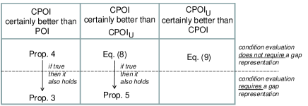
Figure 7: Synopsis of analytical results

Synopsis. Figure 7 illustrates the conditions under which one choice is certainly better (requires less space) than another. Notice that we can check whether some conditions hold or not (specifically those in Prop. 4 and equations (6) and (7)), even if we have a plain POI, i.e. without the need of a gapped representation. On the other hand the conditions that refer to $Gaps(N)$ require having a gapped representation and the value of $Gaps(N)$ depends on the way identifiers have been assigned. However, we can have space savings even if the above conditions are not met, since the conditions rely on lower and upper bounds. This motivates the experimental evaluation of Section 5, where we attempt to compare assignment approaches (aiming at approaching the lower bound of $Gaps(N)$), and investigate the amount of space saving that we can achieve.

4 Assignment Policies for Identifiers

Our objective here is to investigate policies for assigning ids aiming at achieving a small value for $Gaps(N)$. We need a method that takes as input the storage graph of POI and reassigns the ids of triples so that each node to contain ids close to each other. Moreover, that method should be also efficient in time. Below we discuss a number of approaches:

$\bullet$ Default (id assigned at the first appearance of triple). According to this policy, each triple is assigned an id, the first time that it appears in one version, and it gets the smallest available integer. Obviously, this assignment does not depend on the structure of POI.

$\bullet$ Node Size. We order the nodes of the storage graph by their size (i.e. $|n_{i}|$) and then we assign ids to their triples starting either from the larger nodes, or from the smaller nodes. If we start from the larger nodes (Size) then these nodes are favored, so we can expect gains for them. An alternative approach is to start assigning identifiers starting from the smaller nodes (Size_Rev). The motivation is that a small node can “waste” more bits per id, than a large node in a “bad” assignment. Specifically, consider two nodes $n_{i}$ and $n_{j}$ such that $|n_{i}|<|n_{j}|$. We can define the “bits per id of a node $n$” as follows: $bpi(n)=\frac{|gaps(n)|}{|n|}$. The worst (i.e. space consuming) case is $bpi(n)=\frac{|T|-1}{|n|}$. It follows that $worst(bpi(n_{j}))<worst(bpi(n_{i}))$, since $\frac{|T|-1}{|n_{j}|}<\frac{|T|-1}{|n_{i}|}$. By starting from the small nodes, we expect a better assignment for them, an assignment that leads to smaller $bpi(\cdot)$ values. Obviously, nodes with size equal to 1, do not benefit from a gapped representation, therefore we assign identifiers to their triples at the end. In conclusion, each policy (from large or small nodes) has its own pros and cons.

$\bullet$ Triple Frequency. For each triple in $T$ we count the number of nodes that contain it and then we order the triples according to this number, getting a list of the form: $\langle$ appearing $k$ times $\rangle$, $\langle$ appearing $k-1$ times $\rangle$, $\ldots$ , $\langle$ appearing 1 time $\rangle$. Then we assign ids starting from the most frequently occurring triples, aiming at achieving consecutive (or close) ids in several nodes. If we want to reduce the maximum gap between an id and the rest ids, then it is beneficial to assign to that id the value $|T|/2$, since the max gap in that case is $|T|/2$. The ids that can give the maximum gaps (with the rest), are those in the ends of the interval, i.e. $1$ and $|T|$. So one reasonable approach would be to start giving ids to the frequent triples starting by $|T|/2$ and then continue using ids based on their absolute distance from $|T|/2$ (e.g. if $|T|/2=50$, then consume ids in the following order 50,51,49,52,48, and so on). It follows that the least occurring triples will get ids close to 1 or $|T|$. Moreover, note that a triple with $f$=1 does not affect other nodes than the one it appears in, so we do not have to be concerned about the ids of triples with $f=1$ (i.e. no overlapping issues as they appear only in one node). Furthermore, we can exploit the fact that the triples in each frequency list are grouped so that those of the same node are adjacent, for giving them consecutive ids. Finally, if we consider that the distribution of the triples in nodes follows a power-law, then the expected size of the list with $f$=1 is much bigger than the sizes of the other lists. Considering all the above, we start the assignment from the list of triples with $f$=1 and $id=1$. When we have consumed the half of that list, we continue the assignment with the most frequently occurring triples. The rest lists follow (according to their frequency) and at the end we assign the remaining half of triples with $f$=1. This reassignment is more expensive than the previous ones since it requires computing the frequency of all triples.

$\bullet$ Storage Graph. We can traverse the storage graph and assign ids by the order we encounter nodes. Let’s first make some remarks regarding the storage graph: (a) If two nodes are connected (i.e. one is a direct or indirect child of the other) then they certainly have disjoint content. This means that overlaps can occur between nodes which are not connected (and clearly nodes of the same level fall into this category). (b) Each node of the storage graph is pointed to by at least one version. Since the contents of the versions that a node represents equals the triples stored at that node plus the triple stores in all parent nodes of that node, it follows that if the variance of the version contents’ sizes is small, then the maximal nodes of the storage graph (i.e. those which have not any parent), are expected to store more triples than the deeper nodes. Based on the above observations, one approach is to traverse the storage graph in a Breadth-First Search (BFS) manner, i.e. to start from high level nodes and then to descend. In this way it is expected that we will encounter larger nodes at the beginning and such nodes can (is not impossible to) overlap. Alternatively, and with the same motivation with the policy Size_Rev, we could adopt a reverse BFS policy (BFS_Rev). In comparison to Size policy, the storage graph-based policies have the following benefit: successive (during the assignment) nodes have higher probability to have overlaps.

With respect to computational cost, apart from Frequency, the rest reassignment policies do not require any preprocessing, and they are very fast (roughly each method requires traversing the storage graph once).

Example 4.1

Here we explain two of the assignment approaches (Frequency and BFS) through an example. Figure 8 shows the distinct contents of 5 versions and the corresponding graph of POI before and after the adoption of a gapped representation. Now the left part of Figure 9 (resp. right) depicts the procedure of reassignment by Frequency (resp. by BFS). Regarding the former, we first create the frequency lists and then we start the assignment from the list with frequency=1 until the half of that list (in our example we will consume three triples). We continue the assignment with the most frequent triples (i.e. triples appearing in three nodes, in two nodes and finally the remaining two triples of the first list). Subsequently, we update our storage graph with the new ids. The observe that the resulting gapped representation needs less space than the initial graph, specifically even in this small example the space is almost 2.5 times less.

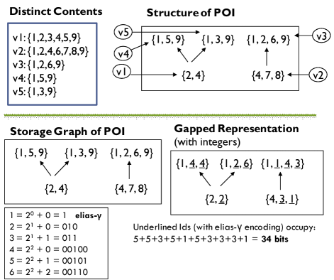
Figure 8: Storage graph of POI without and with a gapped representation

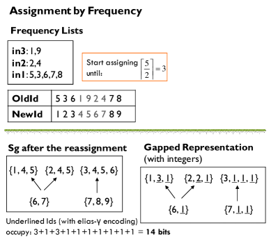
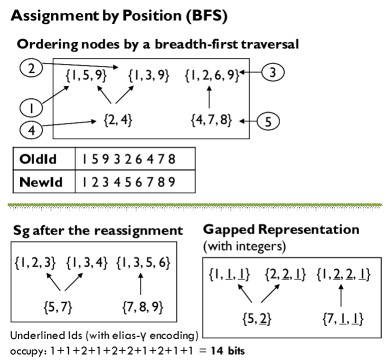
Figure 9: Assignment by Frequency (left) and by BFS (right)

5 Experimental Evaluation

To evaluate the above policies in large datasets we generated and used synthetic datasets. We have to note that related work mainly reports results over synthetic datasets or over real datasets which are not versioned. For these reasons we decided to derive and use three kinds of synthetic datasets.

5.1 Datasets

Dat1. Using the synthetic KB generator described in [21], we created a dataset (Dat1) consisting of 1000 versions, each having 10,000 triples on average, where the size of each triple is 100 bytes (a typical triple size). The version generation method is described next and illustrated in Figure 10. As in real case scenarios, a new version is commonly produced by modifying an existing version. In order to generate the content of a new version, we first choose at random a parent version and then we either add or delete triples from the parent contents. The difference in triples with respect to the parent content is 10%, i.e. 1000 triples. We have an additional parameter $d$ that defines the probability to choose triple additions (so with probability $1-d$ we delete triples). In this respect, we create versions whose contents are either supersets or subsets of the contents of existing versions. We experimented with $d$ in the range of [0.5, 0.9] (we ignored values smaller than 0.5 as deletions usually do not exceed additions). For additions, we assumed that the $25\%$ of the additional triples are triples which already exist in the KB (in the content of a different than the parent version), while the rest $75\%$ are brand new triples. This is motivated by the fact that in a versioning system it is more rare to re-add a triple which exists in an old version and was removed in one of the subsequent versions, than to add new triples. Notice that as $d$ increases, more new triples are created and less are deleted (so the total number of distinct triples increases).

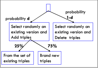
Figure 10: Synthetic dataset generation method for Dat1

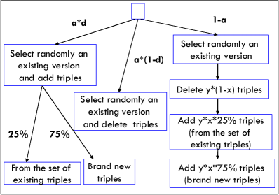
Figure 11: Synthetic dataset generation method for Dat2

Dat2. The Dat1 consists of versions whose contents are proper subset or superset of the contents of the parent versions. To obtain a more realistic dataset, containing less $\subset$ relationships over contents, we created another dataset (Dat2) with a different version generation method illustrated in Figure 11. At first, we choose at random an existing version as a parent and then we either only add or delete triples from the parent content, or we make both triple additions and deletions. In the first case, we create versions whose contents are either subsets or supersets of the contents of existing versions, like Dat1. We have an additional parameter $a$ that defines the probability to choose the first case (and $1-a$ the second case). We experimented with $a$=0.3 (so the probability a version to be proper subset or superset of the parent version is 0.3). In the second case, we add and delete triples from the parent content. We use parameter $x$ to specify the proportion of added triples (and $1-x$ for the deleted triples). The parameter $x$ ranges [0.5, 0.9], so $1-x$ ranges (0.1, 0.5). We used $x=d$ for the production of the dataset used in the experiments. The difference in triples with respect to the parent content is $10\%$ This proportion is represented by the parameter $y$. For additions, in both cases (i.e. $a$ and $1-a$ cases) we assumed that the $25\%$ of the additional triples are triples which already exist in the KB, while the rest $75\%$ are brand new triples. Dat2  consists of 1000 versions, each having 10,000 triples on average as well.

The frequency of triples in versions approximates a power law distribution. This hold for both the frequency of triples in versions, and the frequency of triples in the nodes of POI. Just indicatively, Figure 12 shows in log scale the distribution of triples in versions (left), and in nodes (right) for Dat2 with $d=0.7$ where $|T|=531,500$. Notice that if we exclude the first 10,000 triples the rest 521,500 triples follow a power-law distribution as their plot in the log scale approximates a straight line.

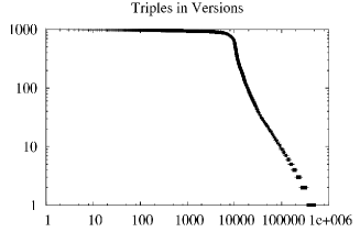
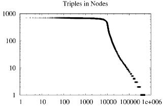
Figure 12: The distribution (in logscale) of triples in versions (up) and in nodes (down) for Dat2 for d=0.7 (Y: frequency, X: triples)

After feeding these datasets to POI we observed that the storage graph of POI for Dat1 has a large number of edges, while the storage graph for Dat2 has a more flat morphology with less connections and depth. Specifically, the average depth of the graph for Dat1 (resp. Dat2) in our experiments (and assuming all $d$ values) is 3 - 5.5 (resp. 1.4), while the max depth for Dat1 (resp. Dat2) is 12 - 14 (resp. 5).

Dat3. This dataset consists of 1000 versions, each having 10,000 triples on average, and $|T|$=400,000. The key characteristics are: no version is subset of another, versions share a lot of common triples and the triple frequency follows a power-law for being close to real datasets (the construction method is detailed in the next paragraph). The dataset is ideal for testing the worst case for POI. Since no version is subset or superset of any other version, the graph of CPOI has a flat structure, i.e. it is like an inverted index where nodes point to compacted lists of triple ids. The only space saving offered by CPOI is that whenever two versions have the same content, only one node and one posting list is kept in CPOI.

The versions of Dat3 were produced as follows: at first we compute the frequency of each distinct triple using the formula $Freq(tripleId)=(\frac{100.230}{tripleId})^{0,6}+25$, meaning that each triple appears to at least 25 versions, creating a list of the form $<$tripleId, #versions$>$. Then we start filling each version’s content consuming the ids of every list consecutively. Specifically, once we have inserted one triple in #versions (according to the list), we continue with the next triple starting insertions from the subsequent version of the one that we added the previous tripleId last.

GO. We also conducted experiments over only a few versions of GO (Gene Ontology). We used the RDF/S dumps from the GO project. This dataset contains 27,640 classes, and 1,359 property instances and uses 126 properties to describe genes. We used only a few versions, specifically 6 versions (v.16-2-2008, v.25-11-2008, v.24-3-2009, v.5-5-2009, v.26-5-2009, v.22-9-2009) which are not successive, so a lot of changes exist between them, and indeed none of them is subset of another. We have to note that if we had used a higher number of versions, then that would be an advantage for CPOI.

5.2 Compared Options

For each dataset we compared the following options:

• plain POI (i.e. no reassignment, 32-bit integer encoding),

• CPOI Default (i.e. no reassignment),

• CPOI after ordering triples randomly (Random),

• CPOI after ordering triples wrt node size (Size in descending order and Size_Rev in ascending order),

• CPOI after ordering triples wrt their frequency in nodes (Frequency),

• CPOI after ordering triples wrt their position in the storage graph (BFS and BFS_Rev for reverse traversal),

• CPOI_U using uniform encoding.
  

We compared the above options with respect to the following aspects: storage space for the node contents, and time to assign the identifiers. For CPOI we tested two encodings: Unary (as it is very close to the analytical results), and Elias-$\gamma$. The latter is better than unary because for an integer $k$, Elias-$\gamma$ requires $2\lfloor\log_{2}k\rfloor+1$ bits, while unary requires $k$ bits.

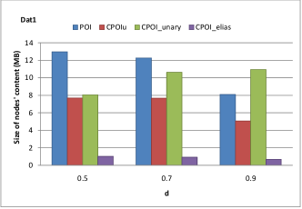
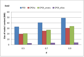
Figure 13: Space for the nodes’ contents for Dat1 (left) and Dat2 (right) of POI, CPOI_U and CPOI (for Unary and Elias-$\gamma$ encoding).

5.3 Experimental Results

[Dat1 and Dat2]
The nodes’ sizes for Dat1 (resp. Dat2) are shown in the left (resp. right) part of Figure 13. It is evident that in both datasets CPOI with Elias-$\gamma$ is by far the best compression method, achieving a 7.5%-8.5% compression ratio. CPOI_U comes second achieving only 59%-63% compression ratio. Third comes CPOI with Unary encoding.

Regarding the $d$ value, since in Dat2 we have less subset or superset relations wrt Dat1, as $d$ increases, $|T|$ and $\sum_{i=1}^{|N|}|n_{i}|$ increases as well, consequently, the required space for POI increases. Regarding CPOI, its space in Dat2 increases, as in Dat1, since it depends on $Gaps(N)$ and for larger $d$ we have larger $|T|$.

Regarding the reassignment policies, Figure 14 shows comparative results for Dat1 and Dat2 using Elias-$\gamma$. In both datasets BFS is the best reassignement (with compression ratio 7.5%-8%), slightly outperforming CPOI Default. The rest reassignment policies are outperformed by CPOI  but none of them is worse than POI or CPOI_U. Figure 16 groups and ranks reassignment policies according to the compression ratio they achieve for each dataset.

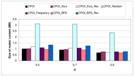
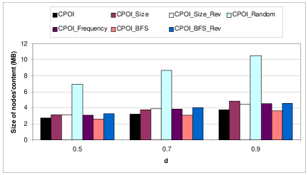
Figure 14: Nodes’s space for Dat1 (left) and Dat2 (right) of CPOI using Elias-$\gamma$ encoding for various assignment policies.

Another interesting observation is that a gapped representation with Elias-$\gamma$ gives around 20% compression ratio (even with a random id assignment). A “good” (i.e. at least not random) assignment (with Elias-$\gamma$ encoding) gives around 8% compression ratio (i.e. three times less space) in comparison to the random assignment.

The time required for the reassignment is short for all policies ranging from 4 to 11 secs for Dat1, and from 14 to 46 secs for Dat2. The fastest policy is BFS, while the slowest is Frequency.

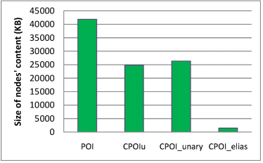
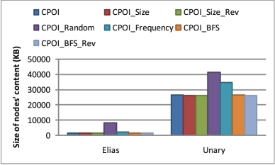
Figure 15: Node space in Dat3.

Figure 16: Ranking of reassignment policies wrt their compression ratio for Elias-$\gamma$ encoding

The main results can be summarized as follows: Using a CPOI with BFS reassignment and Elias-$\gamma$ we can achieve compression ratio of 8% of the size of nodes’ content.

[Dat3]
The results for the nodes’ space are shown in the left part of Figure 15. We can see that CPOI outperforms POI as we expected. CPOI with Elias-$\gamma$ gives the best compression ratio, i.e. 3.5%. CPOI_U comes second achieving 59.4% compression ratio, while CPOI with Unary encoding achieves 63% compression ratio. Regarding the reassignment policies, Figure 15 (right) shows comparative results using Elias-$\gamma$ and unary encoding. The best reassignement is Size_Rev for unary and Size for Elias-$\gamma$ (with compression ratio 62% and 3.3% respectively). Size, Size_Rev and BFS_Rev outperform CPOI Default. The other reassignment policies are outperformed by CPOI Default, but none of them is worse than POI or CPOI_U.

[GO Dataset]
In this dataset, although the graph of POI is again flat, CPOI is better than CB and POI (detailed results are given in the Appendix B).

5.4 Experimental Results vs Analytical Results

Here we discuss the datasets and the experimental results under the light of the analysis of Section 3. The conditions that do not require computing $Gaps(N)$, i.e. those in Prop. 4 and equations (6) and (7), are not satisfied, in none of {Dat1, Dat2, Dat3}, hence by looking at the features of our datasets (i.e. $|n_{i}|,|T|,avg|n_{i}|$) we cannot conclude which approach guarantees space benefits. However, in the GO dataset, the conditions of Prop. 4 and equation (6) hold, so CPOI always guarantee space savings over both POI and CPOI_U. Consequently, the conditions of Prop. 3 and 5, hold too for GO.

Referring to the conditions that require a gap representation (i.e. those in Prop. 3 and Prop. 5), by considering the Default reassignment, Prop. 3 holds for Dat1 for all $d\in[0.5-0.7]$, while for Dat2 for $d\in[0.5-0.9]$. Prop. 5 does not hold for any value of $d$ neither for Dat1 nor for Dat2. Regarding, the other reassignment policies Prop. 3 holds for Dat2 for BFS, Frequency and Size_Rev, while for Size and BFS_Rev it holds only for $d=0.5$. In Dat3 only Prop. 3 holds for all reassignment policies.

These results agree with the experimental results (i.e. the satisfied inequalities also hold in the measured experimental results).

CBD (CB Dictionary-Based approach)

We have included in our experiments also a change-based dictionary approach, for short CBD, in which all deltas contain additions and deletions of identifiers rather than triples. Figure 17 depicts what the CBD approach would store for the versions of the example of Fig. 3-5. In general, this approach is certainly better than CB for those triples of $T$ that occur at least in two deltas. In GO CBD is worse than CB. In Dat3 CBD behaves much better than CB, but worse than CPOI, as shown in the Appendix B. The same happens in Dat2.

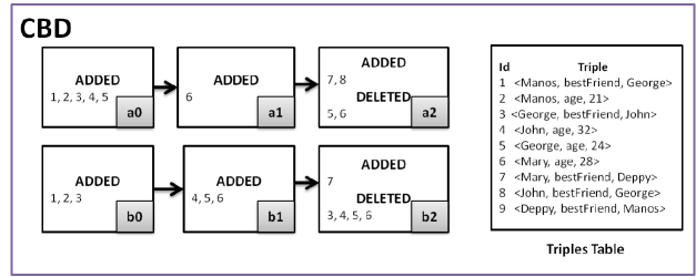
Figure 17: Storing versions according to the CBD approach

5.5 General Discussion & Version Insertion Times

Regarding the comparison of POI (and CPOI) with CBD, in CBD the cost to reconstruct the contents of a version is history dependent (and may more expensive than POI), and POI offers faster subset checking. On the other hand, the addition of a version in CBD can be faster than POI since there is no need for checks to determine its placement in the storage graph. In general we can say that the price to pay, in comparison to IC and CB (as well as CBD), is slower additions of new versions and the adoption of gapped and encoded identifiers makes them slower. Although the insertion algorithm of POI exploits the structure and semantics of the storage graph, its plain version sometimes requires a long time for the addition of a version.

However, the variation with cache which has been proposed in [21], reuses results of set union operations, and leads to an average insertion time less than one second.

In our experiments, the average insertion time for Dat1 (resp. Dat2) was 0.3-0.8 sec (resp. 0.8-1 sec). The gapped and encoded identifiers indeed incurred an overhead, specifically in our experiments for Dat1 (resp. Dat2) the insertion time was 0.8-2.4 sec (resp. 3.2-4.4 sec) which is however an acceptable time. To be more specific, consider a version with $n$ triples. For inserting that version to CPOI, the extra cost (in comparison to POI) is the cost to decode the gapped identifiers of those nodes that will be examined for deciding the right place of the new node that it may have to be inserted in the lattice of CPOI. The extra cost for decoding the identifiers of a node with $n$ triples is linear (in ${\cal O}(n)$) since we have to perform at most one integer addition operation per triple.

Finally we should stress that since a version is added only once, but it can be retrieved unlimited number of times, CPOI is a beneficial choice for the intended application scenario.

6 Possible Applications

Here we describe in brief possible application contexts of CPOI.

• Generic versioning system for RDF/S datasets
  Development for versioning systems (server and client) for RDF/S triple sets, like SVN. The server’s side storage can be based on CPOI.

• Domain-specific archiving solutions.
  In various domains, e.g. in the Marine domain, primary data are kept and updated in relational databases and are periodically exported in RDF/S format according to the LOD (Linked Open Data) best practices. As consequence of this process, past versions of the RDF/S datasets are lost. CPOI can be exploited for versioning these RDF/S datasets mainly those comprised of scientific data over which other experiments take place. In this way the operational database (which is subject of updates) does not need to be enriched with any versioning services.

  In general, one general approach is to adopt a system composed of three subsystems: (a) the operational (transactional) database where updates take place, (b) the latest dataset exported in RDF/S and indexed for offering fast (SPARQL) query services (e.g. it may be stored in a system like RDF-3X [14]), (c) a system based on CPOI that archives and makes accessible the past versions. Note that in case one agent (human or application) would like to browse or query a past version that version can be retrieved from CPOI and expressed in a browsable or queryable system.

  Although the focus on CPOI is archiving, and not time-travel queries or cross version operations, we should note that some operations are very easy and fast to perform over CPOI. Specifically, it is fairly easy and fast to find all versions whose contents are subset (or superset) of a given version, all versions that include or are subset of a given set of triples, etc.

7 Conclusion

We proposed a compact representation for POI  based on gapped representation of triple identifiers and variable-length identifier encodings. We analyzed the space requirements of this representation and identified sufficient conditions that guarantee compression comparing to plain POI. Subsequently, we conducted a large number of experiments over various synthetic datasets, and using several methods for assigning identifiers. The experimental results can be summarized as follows. Regarding identifier assignment policies, we noticed that an assignment in a first-in-first-served basis is almost as good as reassignment policies, and from this we can conclude that identifier reassignment is not necessary. Using a CPOI we can achieve a compression ratio (in comparison to plain POI) of about 8% of the size of nodes’ content. Note that the adoption of a uniform representation (i.e. CPOI_U) would achieve the same compression ratio of 8% if: $\frac{Space_{CPOI_{U}}(N)}{Space_{POI}(N)}=8\%\Leftrightarrow\frac{\lceil\log_{2}|T|\rceil}{\mathbb{B}}=8\%\stackrel{{\scriptstyle\mathbb{B}=32}}{{\Leftrightarrow}}\lceil\log_{2}|T|\rceil=2.56\Leftrightarrow|T|=6$, i.e. if the number of distinct identifiers were only $6$, however in our experiments the number of distinct triples were more than half a million! This demonstrates the benefits of the gapped and specially encoded identifiers.

We have also seen that even in anti-correlated for POI  datasets, CPOI is still better than the CB approach. Finally, we should stress that since we do not deal with the compression of the table that keeps the distinct triple strings and their ids, techniques like those proposed in [14] and [5], are complementary to CPOI and if they are used together will further reduce the overall space.

The price to pay is slower (than IC or CB) insertion times. However note that although a version can be retrieved unlimited number of times, it can be added (i.e. inserted to CPOI) only once. Therefore CPOI is a beneficial choice for the intended application scenario.

At last we should note that apart from RDF/S datasets, CPOI can be a beneficial choice for archiving sets of identifiers. For instance, social networking systems have to keep information about large numbers of users and their memberships to various groups. CPOI could be exploited for versioning such groups.

Appendix A Proofs

The proofs of some propositions follow directly from the discussion and therefore are omitted.

Prop. 1. If a storage graph has $|N|$ sets and they are pairwise disjoint, then: $|T|-|N|\leq Gaps(N)\leq|N|(|T|-|N|)$.

Proof:
If all sets of $N$ are pairwise disjoint (i.e. $n_{i}\cap n_{j}=\emptyset$, $\forall i\neq j,$ $i,j\in[1,|n|]$), then we can achieve the best assignment of identifiers for every node by assigning consecutive ids to the triples of every distinct node. Hence:

$$Gaps(N)\geq\sum_{n_{i}\in N}(|n_{i}|-1)=\sum_{n_{i}\in N}|n_{i}|-\sum_{n_{i}\in N}1=|T|-|N|$$ (8)

On the other hand, the worst assignment in the above case is the one obtained when every node contains triples (ids) that cover the greatest possible range of values. Specifically, the first node will contain the triples with ids 1 and $|T|$ (these will be the min and max ids of that node), and hence, $gaps(n_{1})=|T|-1$ (according to the worst case of a node). Respectively, the second node will include the triples with ids 2 and $|T|-1$ (since every triple occurs only once), and hence, $gaps(n_{2})=(|T|-1)-2=|T|-3$. We can proceed analogously for the rest nodes, so the $k$-th node will contain the triples with ids $k$ and $|T|-(k-1)$, and thus $gaps(n_{k})=(|T|-(k-1))-k=|T|-(2k-1)$. Therefore, $Gaps(N)\leq(|T|-1)+(|T|-3)+...+(|T|-(2|N|-1))$.

$$Gaps(N) \leq (|T|-1)+(|T|-3)+...+(|T|-(2|N|-1))$$

$$= \sum_{i=1}^{|N|}(|T|-(2i-1))=\sum_{i=1}^{|N|}(|T|)-\sum_{i=1}^{|N|}(2i-1)$$

$$= |N||T|-2\sum_{i=1}^{|N|}i+|N|$$

$$= |N||T|-2\frac{|N|(|N|+1)}{2}+|N|\Leftrightarrow$$

$$Gaps(N) \leq |N|(|T|-|N|)$$

$\diamond$

Prop. 2. If a storage graph has $|N|$ sets and there are overlaps then: $\sum_{i=1}^{|N|}|n_{i}|-|N|\leq Gaps(N)\leq|N||T|-|N|$.

Proof:
Let’s consider the case that leads to the worst reassignment for every node. The worst reassignment occurs when every node contains triples (ids) that cover the whole range of values. Specifically, for each node $n_{i}$ we have $gaps(n_{i})=|T|-1$. Note that this case can occur only if the intersection of all nodes $n\in N$ is greater or equal than 2. Consequently, $Gaps(N)\leq|N|(|T|-1)=|N||T|-|N|$. On the other hand, the case that could lead to the best reassignment if overlaps exist, occurs when the intersection between two nodes consists of triples with consecutive ids. Indeed in the first node those ids should be at the beginning of the list, while in the second they should be at the end. For instance, consider four nodes: $n_{1}=\{1,2,3\}$, $n_{2}=\{2,3,4\}$, $n_{3}=\{3,4,5,6\}$, $n_{4}=\{5,6,7\}$. In that case, we can achieve consecutive ids that differ by one, hence:

$$Gaps(N)\geq\sum_{i=1}^{|N|}(|n_{i}|-1)=\sum_{i=1}^{|N|}|n_{i}|-|N|$$

We conclude that in the case that there are overlaps among the nodes’ contents then $\sum_{i=1}^{|N|}|n_{i}|-|N|\leq Gaps(N)\leq|N||T|-|N|$.
$\diamond$

Prop. 4. If the number of distinct triples is not greater than $\mathbb{B}$ times the average number of elements of a node, then CPOI saves space.

Proof:
By combining Prop. 2 and Prop. 3 it follows that we gain with a CPOI if the upper bound of $Gaps(N)$ according to Prop. 2 is less than the right hand of the condition of Prop. 3 (which guarantees gain), i.e. if : right of Prop. 3 $>$ right of Prop. 2.

right of Prop. 3 $>$ right of Prop. 2 $\Leftrightarrow$

$$\mathbb{B}*\sum_{i=1}^{|N|}(|n_{i}|-1)>|N||T|-|N|\Leftrightarrow$$

$$\mathbb{B}*\sum_{i=1}^{|N|}|n_{i}|-\mathbb{B}*|N|-|N||T|+|N|>0\Leftrightarrow$$

$$\mathbb{B}*\sum_{i=1}^{|N|}|n_{i}|-|N|*(|T|+\mathbb{B}-1)>0$$

By expressing $\sum_{i=1}^{|N|}|n_{i}|$ as $|N|*avg(|n_{i}|)$, where $avg(|n_{i}|)$ is the average number of elements of a node, we can write: $\mathbb{B}*|N|*avg(|n_{i}|)-|N|*(|T|+\mathbb{B}-1)>0\Leftrightarrow\mathbb{B}*avg(|n_{i}|)>|T|+\mathbb{B}-1$. The above says that we can always save space with a CPOI when the number of distinct triples is not greater than $\mathbb{B}$ times the average number of elements of a node.

$\diamond$

Prop. 5. CPOI requires less space than CPOI_U, iff $Gaps(N)\leq\sum_{i=1}^{|N|}|n_{i}|*\lceil\log_{2}|T|\rceil-\mathbb{B}*|N|$. $\diamond$

Proof:
CPOI requires less space than CPOI_U when:

$$\mathbb{B}*|N|+Gaps(N)\leq\sum_{i=1}^{|N|}|n_{i}|*\lceil\log_{2}|T|\rceil\Leftrightarrow$$

$$Gaps(N)\leq\sum_{i=1}^{|N|}|n_{i}|*\lceil\log_{2}|T|\rceil-\mathbb{B}*|N|$$

$\diamond$

Prop. 6. The worst case of unary is better than uniform encoding, when: $avg(|n_{i}|)*\lceil\log_{2}|T|\rceil\geq|T|+\mathbb{B}-1$

Proof:

$$\mathbb{B}*|N|+|N|*|T|-|N|\leq\sum_{i=1}^{|N|}|n_{i}|*\lceil\log_{2}|T|\rceil\Leftrightarrow$$

$$\sum_{i=1}^{|N|}|n_{i}|*\lceil\log_{2}|T|\rceil\geq|N|*(|T|+\mathbb{B}-1)\Leftrightarrow$$

$$avg(|n_{i}|)*\lceil\log_{2}|T|\rceil\geq|T|+\mathbb{B}-1$$

$\diamond$

Prop. 7. The best case of unary is worse than uniform encoding, and therefore uniform is certainly better than unary representation, when: $avg(|n_{i}|)*(\lceil\log_{2}|T|\rceil-1)\leq\mathbb{B}-1$

Proof:

$$\mathbb{B}*|N|+\sum_{i=1}^{|N|}|n_{i}|-|N|\geq\sum_{i=1}^{|N|}|n_{i}|*\lceil\log_{2}|T|\rceil\Leftrightarrow$$

$$(\mathbb{B}-1)*|N|\geq\sum_{i=1}^{|N|}|n_{i}|*(\lceil\log_{2}|T|\rceil-1)\Leftrightarrow$$

$$avg(|n_{i}|)*(\lceil\log_{2}|T|\rceil-1)\leq\mathbb{B}-1$$

$\diamond$

Appendix B Total Space

The benefits of CPOI are independent on the size of triple strings, in the sense that the nodes of POI and CPOI store triple indentifiers. However, here we report the results of measurements that include the size of the triple strings just for giving the reader the complete picture. However, and as we stressed in the main body of the paper, one could adopt other complementary techniques for compressing the triple strings themselves (i.e. assign one id for each subject, triple, object of a triple). This means that one could achieve even better compression ratios than those that we report in this section.

[Dat1 and Dat2]
To quantify the overall benefit of using CPOI, we compared the total storage space requirements of IC, CB, POI, CPOI (Elias-$\gamma$ and Default id assignment), and CPOI with the best reassignment policy wrt the experiments (i.e. BFS). For CB we used the symmetric difference operator ($\Delta_{e}$ in [24]), i.e. the difference between two sets of triples $A$ and $B$, is the set $(A\setminus B)\cup(B\setminus A)$.

The upper left (resp. right) part of Figure 18 shows the space requirements for Dat1 (resp. Dat2) in log scale, for various values of $d$ (0.5 - 0.9). We can see that CPOI is always better (the plots of CPOI Default and CPOI BFS coincide since the log scale reduces their difference).

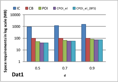
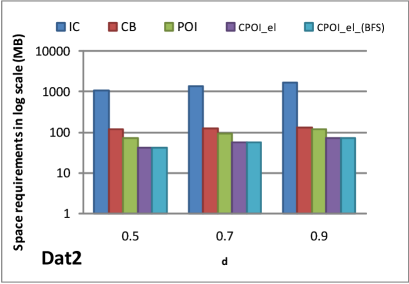
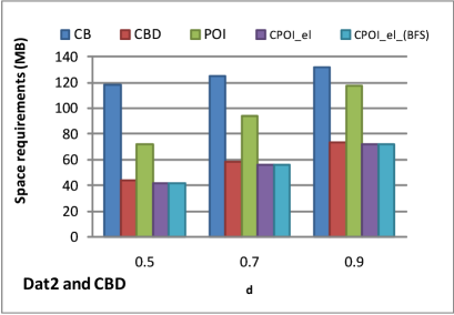
Figure 18: Total space for Dat1(up) and Dat2 (middle) of IC, CB, POI, for various $d$ values. Bottom: Dat2 and CBD

Comparing the total size of CPOI with the other two methods (IC and CB), the former requires only about 4.3% (4.4%-4.8% for Dat1 and 3.8%-4.3% for Dat2) of the space needed for IC  and 35.4%-70.9% (40.1%-70.9% for Dat1 and 35.4%-54.8% for Dat2) of the space needed for CB approach.

[Dat3]
For this dataset the results regarding total space are shown in the Fig. 19. We can see that POI is much better than both IC and CB (as it stores each distinct triple once), while CB is slightly worse than IC.

We conclude that even if no version is subset of another, and we have a significant number of versions, then CPOI is significantly better than the CB approach.

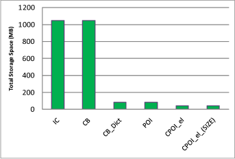
Figure 19: Total storage space in Dat3.

[GO Dataset]
Figure 20 (up) shows comparative results regarding the storage space of nodes. We observe that unary and Elias-$\gamma$ encodings offer significant gains. Now Figure 20 (down) shows the total storage space. We can conclude that even with a few and not subset-related versions, CPOI can be as good as the CB approach (something which is very interesting). Recall that this dataset is ideal for testing the worst case for CPOI since no version is subset or superset of any other version (therefore the graph of CPOI is flat), and the number of versions is very small.

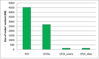
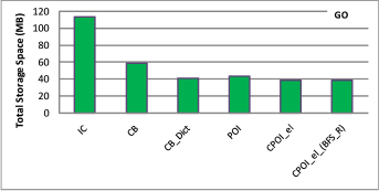
Figure 20: Nodes space and total space in GO

References

- [1] B. Berliner. CVS II: Parallelizing software development. In Procs of the USENIX Winter 1990 Technical Conf., pages 341–352, Berkeley, CA, 1990. USENIX Association.
- [2] T. Berners-Lee. Linked data-the story so far. International Journal on Semantic Web and Information Systems, 5(3):1–22, 2009.
- [3] P. Buneman, S. Khanna, K. Tajima, and W.C. Tan. Archiving Scientific Data. ACM Transactions on Database Systems, 29(1):2–42, 2004.
- [4] P. Elias. Universal codeword sets and the representation of the integers. IEEE Transactions on Information Theory, 21:194–203, 1975.
- [5] J. D. Fernández, M. A. Martínez-Prieto, and C. Gutierrez. Compact representation of large rdf data sets for publishing and exchange. In Procs of the 9th Intern. Semantic Web Conf., ISWC’10, 2010.
- [6] James Geller, Yehoshua Perl, Michael Halper, and Ronald Cornet. Special issue on auditing of terminologies. Journal of Biomedical Informatics, 42(3):407–411, 2009.
- [7] S.W. Golomb. Run Length Encodings. IEEE Transactions on Information Theory, IT-12:399–401, 1966.
- [8] C. Gutierrez, C. A. Hurtado, and A. A. Vaisman. Introducing time into rdf. IEEE Trans. Knowl. Data Eng., 19(2):207–218, 2007.
- [9] M. Hartung, T. Kirsten, and E. Rahm. Analyzing the evolution of life science ontologies and mappings. In DILS, pages 11–27, 2008.
- [10] High Level Expert Group on Scientific Data. Riding the wave — How Europe can gain from the rising tide of scientific data. A report to the European Commission, October 2010.
- [11] T. Kirsten, M. Hartung, A. Gross, and E. Rahm. Efficient management of biomedical ontology versions. In OTM Workshops, pages 574–583, 2009.
- [12] M. Klein, D. Fensel, A. Kiryakov, and D. Ognyanov. Ontology versioning and change detection on the web. In Procs of the 13th European Conf. on Knowledge Engineering and Knowledge Management (EKAW02), pages 197–212. Springer, 2002.
- [13] A. Moffat and L. Stuiver. Binary interpolative coding for effective index compression. Inf. Retr., 3(1):25–47, 2000.
- [14] T. Neumann and G. Weikum. Rdf-3x: a risc-style engine for rdf. PVLDB, 1(1):647–659, 2008.
- [15] T. Neumann and G. Weikum. x-rdf-3x: Fast querying, high update rates, and consistency for rdf databases. PVLDB, 3(1):256–263, 2010.
- [16] N. F. Noy and M. A. Musen. Ontology versioning in an ontology management framework. IEEE Intelligent Systems, 19(4):6–13, 2004.
- [17] J. Ruoming, X. Yang, R. Ning, and W. Haixun. Efficiently answering reachability queries on very large directed graphs. In SIGMOD, pages 595–608, 2008.
- [18] Falk Scholer, Hugh E. Williams, John Yiannis, and Justin Zobel. Compression of inverted indexes for fast query evaluation. In SIGIR, pages 222–229, 2002.
- [19] W. F. Tichy. RCS-A system for version control. Software Practice & Experience, 15(7):637–654, July 1985.
- [20] Y. Tzitzikas and D. Kotzinos. “(Semantic Web) Evolution through Change Logs: Problems and Solutions”. In Procs of the Artificial Intelligence and Applications, AIA’2007, Innsbruck, Austria, February 2007.
- [21] Y. Tzitzikas, Y. Theoharis, and D. Andreou. On storage policies for semantic web repositories that support versioning. In ESWC, pages 705–719, 2008.
- [22] M. Volkel, W. Winkler, Y. Sure, S. R. Kruk, and M. Synak. SemVersion: A Versioning System for RDF and Ontologies. In Procs. of the 2nd European Semantic Web Conf., ESWC’05., Heraklion, Crete, May 29 June 1 2005.
- [23] Ian H. Witten, Alistair Moffat, and Timothy C. Bell. Managing Gigabytes : Compressing and Indexing Documents and Images. Morgan Kaufmann, San Francisco, CA, 2. edition, 1999.
- [24] D. Zeginis, Y. Tzitzikas, and V. Christophides. “On the Foundations of Computing Deltas Between RDF Models”. In Procs of the 6th Intern. Semantic Web Conf., ISWC/ASWC’07, pages 637–651, Busan, Korea, November 2007.