High-harmonic generation in Su-Schrieffer-Heeger chains

Abstract

Su-Schrieffer-Heeger (SSH) chains are the simplest model systems that display topological edge states. We calculate high-harmonic spectra of SSH chains that are coupled to an external laser field of a frequency much smaller than the band gap. We find huge differences between the harmonic yield for the two topological phases, similar to recent results obtained with more demanding time-dependent density functional calculations [D. Bauer, K.K. Hansen, Phys. Rev. Lett. 120, 177401 (2018)]. This shows that the tight-binding SSH model captures the essential topological aspects of the laser-chain interaction (while higher harmonics involving higher bands or screening in the metal phase are absent). We study the robustness of the topological difference with respect to disorder, a continuous phase transition in position space, and on-site potentials. Further, we address the question whether the edges need to be illuminated by the laser for the huge difference in the harmonic spectra to be present.

I Introduction

High-harmonic spectroscopy of condensed matter is an emergent field in strong-field attosecond science, which allows the all-optical probing of structural and dynamical properties Ghimire et al. (2011); Schubert et al. (2014); Vampa et al. (2015); Hohenleutner et al. (2015); Luu et al. (2015); Ndabashimiye et al. (2016); Langer et al. (2017); Tancogne-Dejean et al. (2017); You et al. (2017); Zhang et al. (2018); Vampa et al. (2018); Baudisch et al. (2018); Garg et al. (2018). Topological phases became the focus of research directions such as topological insulators Hasan and Kane (2010); Franz and Molenkamp (2013); Asbóth et al. (2016), topological superconductivity Qi and Zhang (2011); Viyuela et al. (2018), cold atoms Atala et al. (2013), topological photonics Rechtsman et al. (2013); Stützer et al. (2018); Kruk et al. (2019), toplogical electronic circuitry Ningyuan et al. (2015); Albert et al. (2015); Wang et al. (2019), and topological mechanics Kane and Lubensky (2013). Only very recently, the exploration of the physics at the interface between strong-field attosecond science and topological condensed matter began theoretically Koochaki Kelardeh et al. (2017); Bauer and Hansen (2018); Silva et al. ; Chacón et al. ; Drüeke and Bauer ; Ikeda et al. (2018) and experimentally Luu and Wörner (2018); Reimann et al. (2018). Of particular interest there is the all-optical distinction of topological phases, the steering of electrons through Berry curvatures or along topologically protected edges on sub-laser-cycle time scales, with potential applications in coherent light-wave electronics Sommer et al. (2016); Garg et al. (2016); Higuchi et al. (2017); Heide et al. (2018).

In Ref. Bauer and Hansen (2018), harmonic generation in dimerizing linear chains was investigated using time-dependent density functional theory (TDDFT) Runge and Gross (1984); Ullrich (2011). A huge difference in the harmonic yield for the topological phases A and B (see Fig. 1) was observed and attributed to the presence of topological edge states in phase B. The band structures resembled qualitatively those known for the Su-Schrieffer-Heeger (SSH) model Su et al. (1979), originally introduced as a tight-binding model for polyacetylene Streitwolf (1985); Block and Streitwolf (1996) (see Ref. Asbóth et al. (2016) for a modern introduction into the topological aspects of the SSH model).

Figure 1 illustrates the connection between the modelling using the very simple SSH tight-binding approach (leading to two bands only) Su et al. (1979); Streitwolf (1985); Asbóth et al. (2016); Gebhard et al. (1997) and the ab-initio density-functional theory (DFT) on a fine-grained position-space grid Hansen et al. (2017); Bauer and Hansen (2018); Hansen et al. (2018); Yu et al. (2019); Drüeke and Bauer . Let us first consider the upper panel. The atoms are shifted from their equidistant positions (lattice constant $a$) alternatingly by $\delta$ to the right and left, generating the two possible dimerizations called phase A and phase B. For the case of one electron per ion, the equidistant configuration is metallic (half populated lowest band) but energetically less favorable than the dimerized phases (Peierls instability). A band gap opens for phases A and B (metal-to-insulator Peierls transition) because the lattice constant doubles, i.e., the Brillouin zone halves, and the half populated lowest band of the metal becomes a fully populated valence band. Phase B has (for an even number of ions $N$ in the chain) two edge-ions without partner ion to dimerize with. This leads to topological edge states in the band gap between valence and conduction band (see Fig. 1(b-d) in Ref. Bauer and Hansen (2018) for the DFT model).

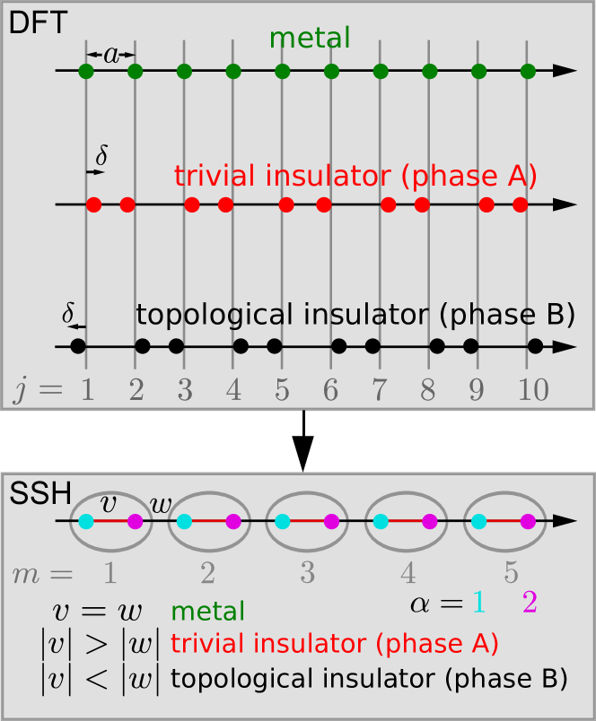
Figure 1: Connection between atom positions on a fine-grained, real-space grid as used in DFT Hansen et al. (2017); Bauer and Hansen (2018); Hansen et al. (2018); Yu et al. (2019); Drüeke and Bauer and the SSH model Su et al. (1979); Streitwolf (1985); Asbóth et al. (2016) to illustrate the discussion in the Introduction.

The lower part of Fig. 1 illustrates the SSH model. The electronic part of the free SSH Hamiltonian [see Eq. (1) or (23)] allows for intra-cell hopping with amplitude $v$ between the two lattice sites $\alpha=1,2$ within a primitive cell $m=1,2,\ldots N/2$, and for inter-cell hopping with amplitude $w$. A connection between the DFT and the SSH model can be established in the spirit of a tight-binding approximation. Both phase A and phase B display two internuclear distances $a-2\delta$ and $a+2\delta$ in the DFT model. As a consequence, the tunneling of electrons between neighboring atoms is more likely for the smaller distance and less likely for the larger. In the SSH model, this is taken into account by the two hopping elements $v$ and $w$. The three cases $v=w$, $|v|>|w|$, and $|w|>|v|$ correspond to metal, phase A, and phase B, respectively. Note that the SSH model describes a bi-partite system because only hopping between sites with different $\alpha$ are allowed.

The SSH model is much simpler than the DFT model. In fact, the SSH model assumes non-interacting electrons and hence reduces to a single-electron problem with only nearest-neighbor hoppings and absent on-site interaction. Because of this simplicity, all the essential features of the SSH model (e.g., band structure, winding number, edge states) can be derived analytically (see, e.g., Asbóth et al. (2016)).

A short introduction to the SSH model and its coupling to an external field are given in section II. In section III, first the harmonic spectra for unperturbed SSH chains are discussed before, in section III.1–III.3, the robustness of the huge difference in the harmonic yield due to topological edge states is investigated with respect to random shifts of the atoms in the chain, a continuous transition between phase A and B in position space, and non-vanishing on-site potential, respectively. Finally, spectra for a hypothetically localized laser field are presented in section III.4 in order to address the question whether the laser needs to illuminate the edges to reveal the huge difference between the two topological phases.

II Theory

II.1 The Su-Schrieffer-Heeger model

The SSH tight-binding Hamiltonian belongs to the wider class of models for dimerized quantum chains Zvyagin (2018). It was originally introduced to describe polyacetylene using a tight-binding description for the $p_{z}$ electrons and elastically coupled CH monomers Su et al. (1979); Streitwolf (1985). We are not interested in the ion dynamics (i.e., phonons) and just consider the electronic part of the SSH Hamiltonian for a given ion configuration. Moreover, we are not thinking of polyacetylene specifically but any 1D chain (or 2 or 3D systems along the laser polarization direction) and thus write $N$ “sites” (instead of $N$ CH monomers). For an even number of sites $N$, the SSH model consists of $n=N/2$ primitive cells with two lattice sites $\alpha=1,2$ each. The real-valued hopping elements $v$, $w$ describe the intra-cell and inter-cell hopping of an electron, respectively. Without external field, the electronic SSH Hamiltonian matrix reads

$$\mathbf{H}_{0}=\begin{pmatrix}0&v&&&&&&\\ v&0&w&&&&\\ &w&0&v&&&&\\ &&v&0&w&&&\\ &&&\ddots&\ddots&\ddots&\\ &&&&w&0&v\\ &&&&&v&0\end{pmatrix}.$$ (1)

This Hamiltonian has $N$ eigenstates

$$\Psi_{i}=\left(\Psi_{i}^{1},\Psi_{i}^{2},...,\Psi_{i}^{j},...,\Psi_{i}^{N}\right)^{\top},$$ (2)

with $i=0,1,...,N-1$ where $\Psi_{i}^{j}$ is the value of the electronic wavefunction at site $j=1,2,\ldots,N$. The electron is on a lattice site with $\alpha=1$ ($2$) if $j$ is odd (even). The Hamiltonian (1) has chiral symmetry Asbóth et al. (2016) and thus a symmetric energy spectrum, i.e., the energies of the eigenstates (in ascending order) fulfill $E_{i}=-E_{N-1-i}$ for $i=0,1,...,N/2-1$.

For periodic boundary conditions (i.e., bulk or rings), the electronic SSH Hamiltonian matrix reads

$$\mathbf{H}_{0}^{(\mathrm{bulk})}=\begin{pmatrix}0&v&&&w\\ v&0&w&&\\ &\ddots&\ddots&\ddots&\\ &&w&0&v\\ w&&&v&0\end{pmatrix}.$$ (3)

Eigenstates for the bulk system can be derived analytically (see appendix A). We choose $v,w<0$ so that the number of nodes in the energy eigenstates increases with energy.

II.2 Position information and coupling to external field

Accepting the hopping elements $v$ and $w$ as free parameters, the electronic SSH model does not require any information about the position of the atoms. However, this information is needed for the coupling to an external field. We make the same choice of the atomic-site positions $x_{j}$ as in Bauer and Hansen (2018) [atomic units (a.u.) $\hbar=|e|=m_{e}=4\pi\epsilon_{0}=1$ are used]:

$$x_{j}=\left(j-\frac{N+1}{2}\right)a-(-1)^{j}\delta,\quad j=1,2,...,N.$$ (4)

Here, $j$ is the atomic-site index, $a$ is the distance between the atoms in the metallic case $\delta=0$, and $\delta\neq 0$ describes the alternating shift of the atoms causing the dimerization (see Fig. 1). We assume that the tunneling probability between neighboring sites scales exponentially with distance and set the hopping elements to

$$v=-\exp[-(x_{2}-x_{1})]=-\exp[-(a-2\delta)],$$ (5)

$$w=-\exp[-(x_{3}-x_{2})]=-\exp[-(a+2\delta)].$$ (6)

For $\delta>0$ ($\delta<0$), the system is in phase A (B). As described in more detail in Ref. Asbóth et al. (2016), the system consists of two bands if $\delta\neq 0$, see Fig. 2 .

For one electron per site, the lower band (valence band) is fully populated while the upper band (conduction band) is empty. The band gap between them increases with the absolute value of $\delta$, independent of the sign. But for $\delta<0$ (phase B) there are two additional states in the middle of the band gap. These almost degenerate states around zero energy are spatially localized at the edges of the chain (hence edge states), one of them being odd, the other even with respect to inversion about the origin $x=0$. In the limit $N\to\infty$ the states become exactly degenerate zero-energy states .

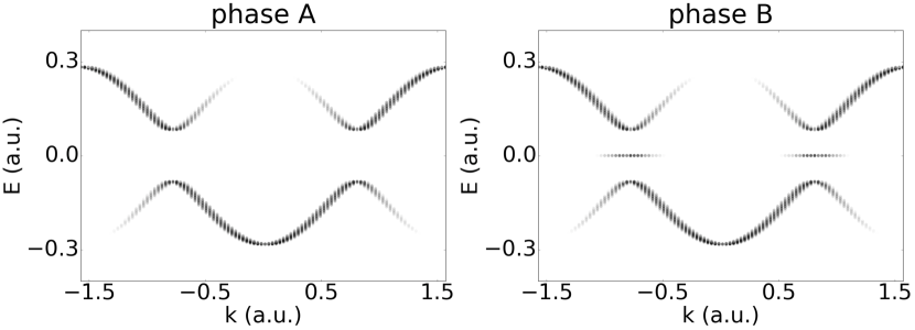
Figure 2: Band structures for $N=100$, $a=2$, and $\delta=0.15$ (trivial-insulator phase A, left) and $\delta=-0.15$ (topological-insulator phase B, right). The first Brillouin zone for the metallic case $\delta=0$ would be $[-\pi/a,\pi/a]$. For the energetically favorable, dimerized case $\delta\neq 0$, the Brillouin zone halves (Peierls instability).

The chain is coupled to a linearly polarized laser field in dipole approximation,

$$\mathbf{A}(t)=A(t)\mathbf{e}_{x},~{}~{}~{}~{}~{}\mathbf{E}(t)=-\partial_{t}\mathbf{A}(t).$$ (7)

The dipole approximation is adequate because we assume that the linear chain is parallel to the laser polarization direction and small compared to the focus of the laser pulse. In Ref. Graf and Vogl (1995), a gauge-invariant coupling of external drivers to tight-binding models was presented. In length gauge, the diagonal elements $H_{jj}$ need to be replaced according

$$H_{jj}=0\longrightarrow-\Phi(x_{j},t)=E(t)x_{j},$$ (8)

whereas in velocity gauge, the hopping elements become

$$H_{jl}\longrightarrow H_{jl}\,e^{-i(x_{j}-x_{l})A(t)}.$$ (9)

In length-gauge, the Hamiltonian matrix thus reads

$$\mathbf{H_{LG}}(t)=\begin{pmatrix}E(t)x_{1}&v&&&\\ v&E(t)x_{2}&w&&\\ &w&E(t)x_{3}&v&\\ &&&\ddots&\\ &&&v&E(t)x_{n}\end{pmatrix}.$$ (10)

For periodic boundary conditions, this implies a discontinuous scalar potential because $E(t)x_{N+1}\neq E(t)x_{1}$. In that case one has to use velocity gauge,

$$\mathbf{H_{VG}}(t)=\begin{pmatrix}0&v^{*}(t)&&&w(t)\\ v(t)&0&w^{*}(t)&&\\ &w(t)&0&v^{*}(t)&\\ &&&\ddots&\\ w^{*}(t)&&&v(t)&0\end{pmatrix},$$ (11)

with

$$v(t) =v\exp[{-i(a-2\delta)A(t)}]$$

$$=-\exp\{-(a-2\delta)[1+iA(t)]\},$$ (12)

$$w(t) =w\exp[{-i(a+2\delta)A(t)}]$$

$$=-\exp\{-(a+2\delta)[1+iA(t)]\}.$$ (13)

One may also use velocity gauge for finite chains without periodic boundary; in that case the upper right and lower left corner elements in (11) are absent. The gauge-invariant coupling in velocity gauge proposed in Ref. Graf and Vogl (1995) reduces to the usual Peierls substitution in our case with dipole approximation (see appendix C).

II.3 Numerical calculations

The eigenstates of the $N$-dimensional SSH Hamiltonian (1) are obtained by diagonalization. The $N/2$ lowest energy states (occupied by $N$ electrons, assuming spin degeneracy) are propagated in time from the beginning to the end of a laser pulse. An $n_{\mathrm{cyc}}=5$-cycle sine-squared laser pulse is used with

$$A(t)=A_{0}\sin^{2}\left(\frac{\omega t}{2n_{\mathrm{cyc}}}\right)\sin\omega t,~{}~{}~{}0<t<2\pi\omega/n_{\mathrm{cyc}}$$ (14)

and zero otherwise. The electric field follows from (7). The frequency is set to $\omega=0.0075$ (i.e., $\lambda\simeq 6.1\,\mu$m), and the vector potential amplitude is $A_{0}=0.2$ (corresponding to a laser intensity of $\simeq 7.9\times 10^{10}$ Wcm^-2) throughout the paper. The results discussed in this paper are qualitatively insensitive to the details of the laser pulse as long as $A_{0}$ is large enough to yield high harmonics at all, and the laser frequency is small compared to the band gap.

Wavefunctions are propagated in time using the Crank-Nicolson approximant to the time-evolution operator

$$\exp[-i\mathbf{H}(t)\Delta t]=\frac{1-i\mathbf{H}(t)\Delta t/2}{1+i\mathbf{H}(t)\Delta t/2}+{\cal O}(\Delta t^{3}),$$ (15)

where the discrete time step is set to $\Delta t=0.1$. High-harmonic spectra for the finite chains may be calculated from the dipole, the acceleration, or the current Bandrauk et al. (2009); Baggesen and Madsen (2011), differing by prefactors $\omega^{4}$ or $\omega^{2}$, respectively. Apart from the sign, the position expectation value equals the dipole and reads

$$X(t)=\sum_{i=0}^{N/2-1}\sum_{j=1}^{N}\Psi_{i}^{j*}(t)x_{j}\Psi_{i}^{j}(t)$$ (16)

where $i$ labels the state and $j$ the position. Semi-classically and for uncorrelated emitters, the spectrum of the radiated light $P(\omega)$ is proportional to the absolute square of the Fourier-transformed dipole acceleration Sundaram and Milonni (1990),

$$P(\omega)\propto\left|\mathrm{FFT}\left[\ddot{X}(t)\right]\right|^{2}.$$ (17)

We normalize the spectra to the maximum of

$$P_{\mathrm{free}}(\omega)=\left|\mathrm{FFT}\left[E(t)\right]\right|^{2}.$$ (18)

Since for bulk calculations with periodic boundary conditions the dipole is not defined and the length gauge cannot be used, harmonic spectra were determined from the current $I(t)$ in velocity gauge as $P(\omega)\propto\left|\mathrm{FFT}\left[I(t)\right]\right|^{2}$. However, there is no difference between harmonic spectra $P(\omega)$ from phase A and phase B for periodic boundary conditions. On one hand, one may expect this because phase A and B look alike for periodic boundary conditions. On the other hand, one may expect a difference because of the bulk-boundary correspondence Hasan and Kane (2010); Rhim et al. (2018). We address this issue in section III.4.

III Results

Consider a chain with $N=100$ sites, $a=2$, and $\delta=0.15$ (phase A), $\delta=-0.15$ (phase B). We will focus on this specific chain configuration throughout the paper if not stated otherwise. For the sake of completeness, we also consider the metallic case $\delta=0$. The corresponding harmonic spectra for the laser pulse (14) are presented in Fig. 3. Similar to the results obtained with TDDFT Bauer and Hansen (2018), we find a huge difference in the harmonic yield for phases A and B for harmonic orders smaller than the band gap $\Delta E_{gap}$, corresponding to harmonic order $\simeq 22$. Harmonics above the band gap are so-called inter-band harmonics and produced in the usual three-step way known from the gas phase Vampa and Brabec (2017): an electron tunnels into to the conduction band, electron and hole move in the conduction and valence band, respectively, and recombine when they meet in position space, upon emission of harmonic radiation. The ultimate highest harmonic in a tight-binding system such as the SSH model thus is the maximum energy difference between valence and conduction band, which is $\Delta E_{\max}\simeq 0.566$ for phases A and B, and $0.541$ for the metal. In terms of harmonic orders this corresponds to $\Delta E_{\max}/\omega=75.4$ and $72.2$, respectively, which agrees with the ultimate cut-offs in Fig. 3. If higher conduction bands are taken into account (as done in TDDFT simulations), harmonics beyond these cut-offs can be generated. Below the band gap (i.e., for harmonic orders $<22$), the harmonic yield for phase A drops because the efficient three-step mechanism cannot produce harmonics at such low energies. Only clean intra-band harmonics for orders $\leq 9$ are observed, which originate from the motion of electrons in the non-parabolic regions of the valence band. For phase B, we find high-harmonic yield down to harmonic order $11$, which corresponds to the energy difference between the valence band and the edge states (half the band gap of phase A). These low harmonics can be generated via electronic transitions between edge states and valence band. Below harmonic order $11$, the yield for phase B decreases a bit before intra-band harmonic generation takes over, as in phase A.

Intra-band harmonics from a fully populated valence band tend to interfere away because in such a simple band structure as the one for the SSH chain, for each valence-band electron initially located at a $k$-point with a certain band curvature there is another electron with the opposite band curvature. Such pairs of electrons oscillate with opposite excursions when driven by the laser field so that their dipole radiation interferes destructively. That is the reason why the intra-band harmonics drop rapidly with the harmonic order both for phase A and B in Fig. 3. However, from harmonic order $11$ on, transitions to the edge states come into play for phase B, and the harmonic yield increases again. For phase A, inter-band harmonic generation only sets in towards band-gap harmonic order 22. As a consequence, a huge difference in the harmonic yield for harmonic orders $\in[\Delta E_{\mathrm{gap}}/2\omega,\Delta E_{\mathrm{gap}}/\omega]$ arise, explaining the observations obtained with TDDFT in Ref. Bauer and Hansen (2018) but with a simpler tight-binding model. The differences for energies above the band gap up to order $\approx 40~{}(\approx\Delta E_{max}/2\omega=38)$ are also due to the edge states present in phase B. With edge states in the band gap, transitions to the conduction band are more likely, leading to a higher harmonic yield for phase B.

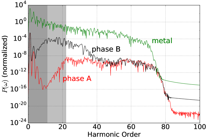
Figure 3: Harmonic spectra for the two topological phases A and B, and the metallic case. The lighter gray-shaded area indicates harmonic photon energies smaller than the band gap for phase A, the darker gray-shaded area indicates energies below the gap between bands and edge states in phase B. The harmonic yield $P(\omega)$ is normalized to $P_{\mathrm{free}}(\omega)$, eq. (18).

For completeness, the spectrum for the metallic phase is plotted in Fig. 3 as well. The metal has no band gap and only a single, half-occupied band so that the cancellation due to opposite band curvature does not take place. As a result, one observes efficient harmonic generation up to the ultimate cut-off energy. However, because of the absence of screening in the SSH model this is not a realistic description of harmonic generation in a metal. In fact, the spectrum for the metal case obtained with TDDFT in Bauer and Hansen (2018), where screening is taken into account, does not show efficient harmonic generation .

For periodic boundary conditions (i.e., bulk or a ring chain) the spectra for both phases are identical and the dip below the band gap is comparable to the one of phase A in a finite chain.

The hopping elements as a function of the distance between neighboring atomic sites are defined in eqs. (5) and (6). In the following, we initialize the atomic-site positions in various ways that deviate from the pure, dimerized cases A and B in order to study the robustness of the band structure and the harmonic spectra for the respective configurations.

III.1 Random shifts

Starting from the pure phase-A case with $\delta=0.15$, we shift each atom from its original position $x_{i}^{0}$ by a random $\Delta x_{i}$ to $x_{i}=x_{i}^{0}+\Delta x_{i}$ in order to investigate the influence of disorder on the harmonic spectra. These random shifts cause a modification of the hopping amplitudes. The rate to jump from atom $i$ to $i+1$ (and back) is given by

$$t_{i,i+1}=t_{i+1,i}=-\exp[-|x_{i+1}-x_{i}|].$$ (19)

The random shifts obey a normal distribution of variance $\sigma$. We calculate averaged spectra for $\sigma=0.1$ and $0.2$ with ensembles of 100 configurations each. The averaged spectra are shown in Fig. 4 (a), together with the unperturbed case $\sigma=0$ for reference.

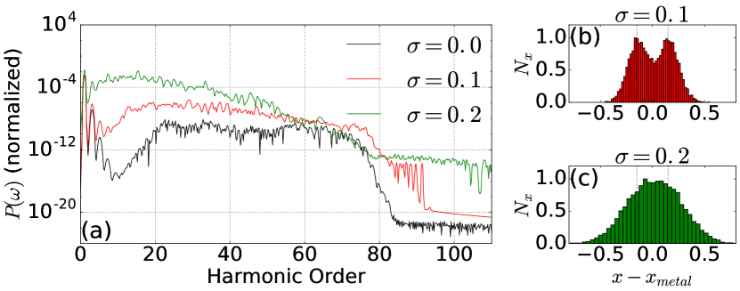
Figure 4: (a) Averaged harmonic spectra over 100 ensembles of randomly shifted atomic sites with respect to the unperturbed phase-A configuration for $\delta=0.15$. The shifts follow a normal distribution of variance $\sigma$. Panels (b) and (c) show the deviations of $x_{i}$ from the metallic case $x_{metal}$ as histograms. For the unperturbed phase A, all values would be located at $\pm\delta=\pm 0.15$, indicated by vertical dashed lines.

A decreased harmonic yield at low harmonic orders for a variance $\sigma=0.1$ can be still observed while the dip disappears for $\sigma=0.2$. The deviations of the atomic positions from the metal case are shown in Fig. 4 (b) and (c) as histograms. For the pure phase A the deviations are either $-\delta=-0.15$ or $+\delta=+0.15$. The distribution for $\sigma=0.1=2\delta/3$ is already quite broadened but two maxima are still clearly visible. For $\sigma=0.2$, the atom positions are too random to yield two maxima in histogram.

The energies of the states explain some features of the spectra. With increasing $\sigma$, the maximum energy difference in general increases, causing a higher ultimate cut-off in the spectrum. In addition, the band gap closes. The disappearance of the dip in the spectrum for larger variances is therefore caused by the disappearing band gap. However, this closing of the band gap due to disorder happens surprisingly slowly as a function of increasing $\sigma$. For a variance $\sigma=0.1=2\delta/3$, the band gap is still clearly visible, and the dip in the harmonic spectrum of phase A is thus remarkably robust against disorder in the atomic positions.

The same happens for phase B (not shown) although the dip there is less pronounced in the first place because of the edge states that effectively halve the band gap.

III.2 Phase transition

A topological phase transition is characterized by an abrupt change in a topological invariant. For the SSH model, the winding number introduced in appendix B serves as such a topological invariant. In position space, such a topological phase transition might be continuous. Consider pure phase B ($N=100$, $\delta=-0.15$, $a=2.0$). We may continuously transform the system from phase B to phase A by moving the left-most atom (original position $x_{1}=-99.15$) to the right $x_{1}=100.85$, as sketched in Fig. 5. The eigenenergies are calculated for many configurations with $x_{1}\in[-99.15,100.85]$ and plotted vs $x_{1}$ in Fig. 6. The hopping elements are obtained by equation (19).

Figure 5: Illustration of the continuous phase transition between the dimerized chain in phase B to phase A in position space (for better visibility only $N=10$ atoms are considered). The filled circle indicates the moving atom whose position is $x_{1}$. The other circles indicate the fixed atoms.

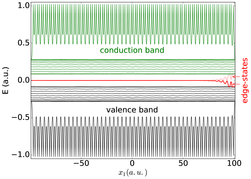
Figure 6: SSH eigenenergies as a function of the position $x_{1}$ of the shifted ion that is originally at the left edge. The energies of the two initially degenerate edge states depart only from $E=0$ when $x_{1}$ is already close to the right edge.

One observes that mainly the lowest, the highest, and the two edge-state energies are affected. The groundstate energy is minimum if the moving atom is on top of another atom (with exceptions at the edges though). For pure phase B, the edge-state energies are almost zero. In phase A, there are no edge-states, so that during the transition the degeneracy of the edge states is lifted. One edge state joins the valence band from above, the other the conduction band from below. It might be surprising that the degeneracy is removed only at an $x_{1}$-value quite close to the final phase-A position while the inversion symmetry is broken already for small shifts away from the pure phase-B configuration.

In phase B, electrons occupying the edge states are localized at the edges, as seen in Fig. 7(a). The left-edge part of the wavefunction moves with the moving atom whereas the right-edge part stays at the right edge. Plotting the energy difference between the edge states vs $x_{1}$ logarithmically [see Fig. 7(c)], reveals an exponential increase. As the left part of the wavefunction moves towards the right side, the overlap with the right-edge part increases exponentially, which leads to the observed exponential increase of the energy difference. A local maximum is observed whenever the moving atom is located at the position of another atom on sub-lattice site $\alpha=2$. There, the wavefunction parts from the left and right interfere destructively so that for $x_{1}$ close to the final position at the right edge the entire wavefunction becomes delocalized.

So far, we considered only two particular dimerization shifts $\delta=\pm 0.15$. With increasing $\delta$, the two hopping elements $v$ and $w$ differ more, and the edge states in phase B become more and more localized at the edges with a smaller and smaller energy difference. As a result, the slope of the energy difference with increasing $x_{1}$ is larger [see Fig. 7(c)].

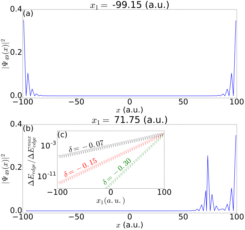
Figure 7: Probability density for edge state $\Psi_{49}$ for different positions $x_{1}$. The inset shows the energy difference between the edge states (for different $\delta$) as a function of $x_{1}$.

As seen above, harmonic spectra for pure phase A have a strong dip for photon energies below the band gap while those from phase B have a weaker dip for energies below the difference between edge state energy and the bands. The weak dip is observed up to about $x_{1}\simeq 35$, as seen in Fig. 8(a) for $x_{1}=33.75$. The dip is “filled up” for larger $x_{1}$ due to an increased yield for low harmonic photon energies generated by transitions between the edge states (see spectrum for $x_{1}=71.75$). If one neglects the edge states in the calculation of the harmonic spectrum, the dip is still there. The time evolution of the initially occupied edge-state orbital in the laser field is presented in Fig. 8(b) and shows a charge transfer between the right edge and the position of the shifted atom due to transitions to the other (initially not populated) edge state and back .

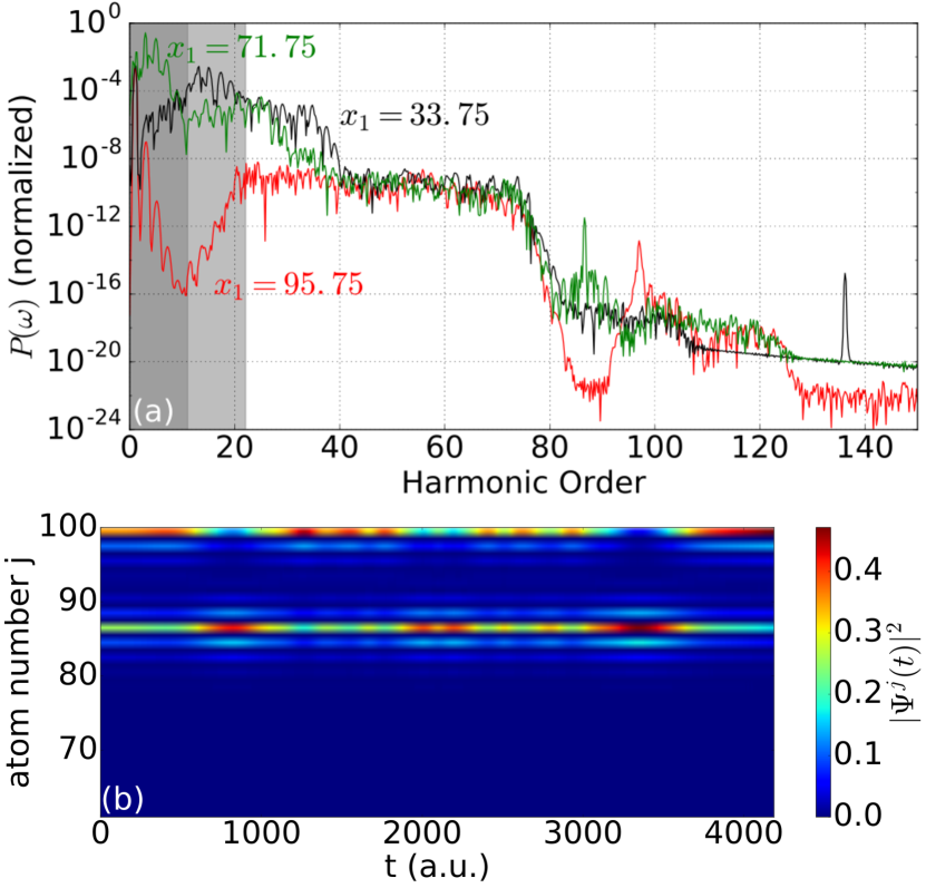
Figure 8: (a) Harmonic spectra for different positions of the shifted atom $x_{1}$. (b) The time evolution of the probability density of the occupied edge state during the laser pulse for $x_{1}=71.75$.

The former edge states become delocalized once their energies are shifted close to the bands. Then the overall spectrum shows already the phase-A-like strong dip in the sub-band-gap region, as seen in Fig. 8(a) for $x_{1}=95.75$. Neglecting the contribution of the former occupied edge state yields a spectrum without the dip for those energies because of incomplete destructive interference of all the dipoles.

Due to the separation of the ground state $\Psi_{0}$ (and the highest state $\Psi_{99}$) from the valence band (conduction band) (see Fig. 6) additional features appear in the spectrum beyond the cut-off.

III.3 Non-vanishing on-site potential

An on-site potential leads to diagonal elements in the Hamiltonian matrix. If all diagonal elements are set to the same value $\epsilon$, the eigenfunctions $\Psi_{i}$ remain the same, and all eigenenergies $E_{i}$ are shifted by $\epsilon$. Harmonic spectra remain unaffected by such a trivial shift of the energy scale. If the diagonal elements are normally distributed random numbers, the bandstructure is smeared out. We found that up to a variance of $\sigma\simeq 0.05$, the dip in phase A can still be observed.

More interesting is a sine-shaped profile for the diagonal elements $\epsilon_{j}$,

$$\epsilon_{j}=\epsilon_{0}\sin(2\pi\nu j/N),$$ (20)

which might be viewed as a generalization of the Rice-Mele model Rice and Mele (1982). For, e.g., $\nu=1/2$ and $\epsilon_{0}=0.1$, the mean value of the $\epsilon_{j}$ is larger than zero so that the eigenenergies are shifted to higher values. These shifts depend on the unperturbed energy of the state, lower-energy states in each band are shifted less than higher-energy states, which leads to a separation of states from the bottoms of the bands (see Fig. 9). The chiral symmetry is broken. The separated states are pairwise degenerate. The original edge states in phase B remain close to $E=0$ and thus enter the valence band around $\epsilon_{0}=0.09$. For phase A, a dip in the harmonic spectrum is still observable because of the presence of a band gap (not shown).

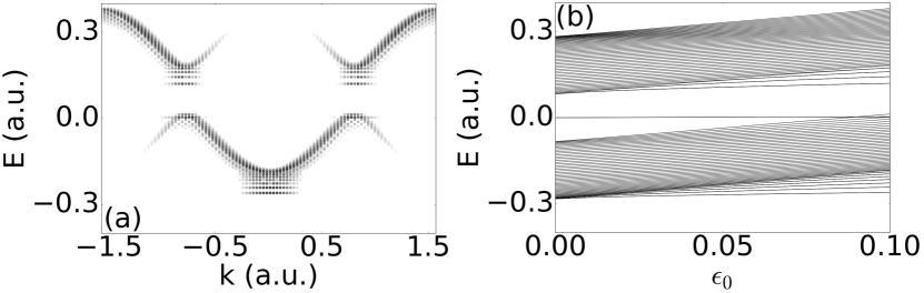
Figure 9: (a) Band structure for phase B with diagonal elements of frequency $\nu=1/2$ and $\epsilon_{0}=0.1$. (b) Eigenenergies as a function of $\epsilon_{0}$.

For more oscillations $\nu$ in the diagonal elements, a new periodicity is enforced on the system that increases the lattice constant (i.e., decreases the Brillouin zone) and increases the number of atoms per primitive cell. For phase A, the bandstructure and the high-harmonic spectrum is shown in Fig. 10 for $\nu=10.5$ as well as the evolution of the energies with increasing $\epsilon_{0}$. One observes a separation of the two bands into subbands. The chiral symmetry of the energy spectrum about $E=0$ is broken [compare, for example, the second lowest and the second highest band in Fig. 10(a,b)]. Nevertheless the characteristic dip for harmonic spectra from phase A is observed because a band gap between highest occupied orbital and lowest unoccupied still exists.

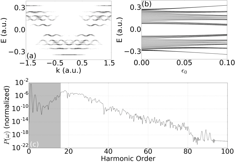
Figure 10: (a) Band structure for phase A with diagonal elements of frequency $\nu=10.5$ and $\epsilon_{0}=0.1$. (b) Eigenenergies as a function of $\epsilon_{0}$. (c) High-harmonic spectrum for $\nu=10.5$ and $\epsilon_{0}=0.1$.

III.4 “Measurable” bulk-boundary correspondence?

Up to now, a laser pulse with the same intensity over the whole chain was applied. Now the laser is focused at certain areas of the chain according to

$$E(x,t)=E(t)\cos^{2}\left(\frac{(x-x_{0})\pi}{2~{}x_{l}}\right)$$ (21)

for $|x-x_{0}|<x_{l}$ and zero otherwise. Here, $E(t)=-\partial_{t}A(t)$ is the previously used pulse shape in time. Note that such a tight focussing is impossible in practice because the wavelength $\lambda\simeq 6.1~{}\mathrm{\mu m}$ of the laser is large compared to the size of the chain ($9.9~{}\mathrm{nm}$). However, we are interested in a gedankenexperiment related to the bulk-boundary correspondence Hasan and Kane (2010); Rhim et al. (2018). It is known that topological invariants (i.e., in our case the winding number introduced in appendix B) are a bulk property while the presence of edge states in the band structure requires actual boundaries. Recently, it has been demonstrated for the Haldane model that the topological invariant (the Chern number) is imprinted in the phases of harmonics emitted from the bulk Silva et al. . However, the harmonic feature of interest in our work is the dip or its absence in the sub-band-gap harmonics for phase A and B, respectively. All our explanations relied on the presence of edge states in the band structure so that we do not expect a difference for phases A and B if the edges are not illuminated by the laser. In other words, our observable is not sensitive to the winding number but to the edge-state levels in the band structure, as is demonstrated in the following.

Using length gauge, the diagonal elements are replaced by

$$\epsilon_{j}=\int_{0}^{x_{j}}E(x,t)\,dx.$$ (22)

First, the laser pulse is focused on the center of the chain $x_{0}=0$, illuminating 10 atoms ($x_{l}=10$), as indicated in Fig. 11(a). The harmonic spectra for the two phases are almost identical and shown in Fig. 11(b). Especially the strong dip in the sub-band-gap region as the key feature of phase A is now also observed in phase B.

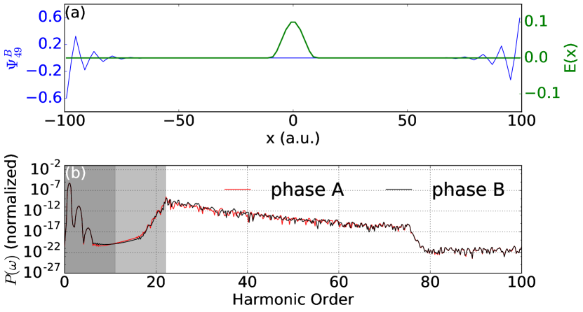
Figure 11: (a) Occupied edge-state of phase B and the artificially narrow focus of the laser pulse in the center of the chain. (b) High-harmonic spectra for phase A and B with the localized laser field in the center of the chain.

The dip is caused by destructive interference of the individual dipoles of all electrons in the valence band. The edge states in the band gap present in phase B are responsible for the fact that the dip is much weaker in phase B and at approximately half the energy. A laser illuminating only the center of the chain does not cause transitions to the edges states so that the dip is then as strong as in phase A.

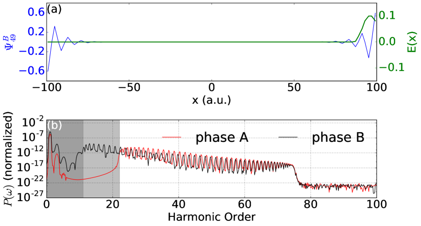
Figure 12: (a) Occupied edge-state of phase B and the artificially narrow focus of the laser pulse on the right edge of the chain. (b) High-harmonic spectra for phase A and B with the localized laser field at the right edge of the chain.

As the focus of the laser is moved towards the edges, the harmonic spectra of phase A and B become different. With the focus on, e.g., the right edge, transitions between edge states and other states become possible, which leads to harmonic spectra that are qualitatively similar to the uniformly illuminated chains, see Fig. 12.

IV Summary

High-harmonic generation in the different topological phases of Su-Schrieffer-Heeger chains was studied. The laser frequency was small compared to the band gap. In this regime, the overall features in the harmonic spectra can be explained using the common three-step model for the emission of harmonics above the band gap. Below-band-gap harmonics are strongly suppressed, causing dips in the harmonic spectra. Because of edge states in the middle of the band gap for the topological phase B, the dip is narrower, at lower harmonic orders, and less pronounced compared to phase A. As a result, a many-order-of-magnitude difference in the sub-band-gap harmonic yield between phase A and B is observed. Our results for the laser-driven SSH chain in tight-binding approximation confirm previous findings with more demanding time-dependent density functional theory simulations Bauer and Hansen (2018). Differences arise in the spectra for the metal phase (due to the absence of screening in the SSH modelling) and because of the absence of high harmonics beyond the maximum energy difference between the energy levels of the SSH Hamiltonian. A remarkable robustness of the spectral features with respect to disorder in the atomic positions, a continuous transition from phase B to phase A in position space, and a modulated on-site potential was found. Further, we demonstrated that the edges need to be illuminated in order to see different harmonic spectra for phase A and phase B. However, this is not in contradiction with the bulk-boundary correspondence; rather our observable is sensitive to the presence or absence of edge states in the band structure but not to the winding number.

Appendix A Analytical solution for the bulk Hamiltonian

For the Hamiltonian of the bulk system (i.e., periodic boundary conditions) given in equation (3), the analytical solution can be derived Asbóth et al. (2016). Rewriting the Hamiltonian in bra-ket notation gives

$$\begin{split}\hat{H}_{0}^{\mathrm{(bulk)}}=&v\sum_{m=1}^{n}\left(\ket{m,2}\bra{m,1}+\mathrm{h.c.}\right)\\ &+w\sum_{m=1}^{n}\left(\ket{m,2}\bra{m+1,1}+\mathrm{h.c.}\right)\end{split}$$ (23)

where $n=N/2$, and $\ket{n+1}=\ket{1}$. We assume the hopping elements to be real-valued. The time-independent Schrödinger equation

$$\hat{H}_{0}^{\mathrm{(bulk)}}\ket{\Psi}=E\ket{\Psi}$$ (24)

can be solved by the Bloch-like ansatz

$$\begin{split}\ket{\Psi_{i}(k)}&=\ket{k}\otimes\ket{u_{i}(k)}\\ &=\frac{1}{\sqrt{n}}\sum_{m=1}^{n}e^{imk}\ket{m}\otimes\sum_{\alpha=1,2}g_{i}^{\alpha}(k)\ket{\alpha},\end{split}$$ (25)

leading to

$$\begin{split}E_{i}(k)\ket{\Psi_{i}(k)}&=\frac{1}{\sqrt{n}}\sum_{m=1}^{n}e^{imk}\left[vg_{i}^{1}(k)\ket{m,2}\right.\\ &\quad+vg_{i}^{2}(k)\ket{m,1}+wg_{i}^{1}(k)\ket{m-1,2}\\ &\quad\left.+wg_{i}^{2}(k)\ket{m+1,1}\right].\end{split}$$ (26)

Multiplying by $\bra{m^{\prime}}$ from the left gives

$$\begin{split}E_{i}(k)\ket{u_{i}(k)}&=E_{i}(k)\left(g_{i}^{1}(k)\ket{1}+g_{i}^{2}(k)\ket{2}\right)\\ &=vg_{i}^{1}(k)\ket{2}+vg_{i}^{2}(k)\ket{1}\\ &\quad+wg_{i}^{1}(k)e^{ik}\ket{2}+wg_{i}^{2}(k)e^{-ik}\ket{1},\end{split}$$ (27)

and in matrix representation

$$E_{i}(k)\mathbf{u}_{i}(k)=\mathbf{H}(k)\mathbf{u}_{i}(k),$$ (28)

with the Bloch-Hamiltonian and vector

$$\mathbf{H}(k)=\begin{pmatrix}0&v+we^{-ik}\\ v+we^{ik}&0\\ \end{pmatrix},\quad\mathbf{u}_{i}(k)=\begin{pmatrix}g_{i}^{1}(k)\\ g_{i}^{2}(k)\\ \end{pmatrix},$$ (29)

respectively. The dispersion relation for the SSH-bulk

$$\begin{split}E_{\pm}(k)&=\pm\sqrt{(v+we^{-ik})(v+we^{ik})}\\ &=\pm\sqrt{v^{2}+w^{2}+2vw~{}\mathrm{cos}~{}k}\end{split}$$ (30)

follows. For either $v=0$ or $w=0$, the chain decomposes into $n$ independent dimers with energy values $\pm v$ or $\pm w$, independent of $k$ (flat bands). If $v$ and $w$ have the same sign, the smallest band gap is located at the Brillouin-zone boundaries $k=\pm\pi$. Note that for $v$ and $w$ having different signs, the shape of the bands stay the same but they are shifted by $\pi$ along $k$. We assume in the following that $v$ and $w$ are equally signed. The value for the smallest band gap is then

$$\Delta E=E_{+}(k=\pi)-E_{-}(k=\pi)=2\left|v-w\right|.$$ (31)

For the metallic case $v=w$, the band gap disappears. Normalized eigenvectors are

$$\mathbf{u}_{\pm}(k)=\left(g_{\pm}^{1}(k),g_{\pm}^{2}(k)\right)^{\top}=\frac{1}{\sqrt{2}}\left(1,\frac{E_{\pm}(k)}{v+we^{-ik}}\right)^{\top}.$$ (32)

The lowest and highest energies are

$$E_{\min}=E_{-}(0)=-\left|v-w\right|,$$ (33)

$$E_{\max}=E_{+}(0)=\left|v-w\right|,$$ (34)

respectively. Insertion into the ansatz (25) yields the corresponding states

$$\ket{\Psi_{\pm}(0)}=\frac{1}{\sqrt{2n}}\sum_{m=1}^{n}\left(\ket{m,1}\pm\mathrm{sgn}(v+w)\ket{m,2}\right).$$ (35)

Appendix B Winding number

The $2\times 2$ Bloch-Hamiltonian (29) can be written in the form Asbóth et al. (2016)

$$\mathbf{H}(k)=\mathbf{d}(k)\cdot\bm{\sigma},$$ (36)

where $\bm{\sigma}=(\bm{\sigma}_{x},\bm{\sigma}_{y},\bm{\sigma}_{z})^{\top}$ is the vector of Pauli-matrices and $\mathbf{d}(k)=\left(d_{x}(k),d_{y}(k),d_{y}(k)\right)^{\top}$ is a 3-dimensional vector, parametrized by $k$. By comparing real and imaginary parts of the Hamiltonian in (29) and (36) one finds

$$\mathbf{d}(k)=\left(v+w~{}\mathrm{cos}(k),w~{}\mathrm{sin}(k),0\right)^{\top},$$ (37)

describing a circle of radius $|w|$ in the $d_{x}d_{y}$-plane, centered at $(v,0,0)^{\top}$. The winding number is defined as the number of times the origin is encircled counter-clockwise as $k$ goes, e.g., from $-\pi$ to $\pi$. Depending on the ratio of $v$ to $w$ and their signs, the winding number can be either $-1$ (a single clockwise encircling of the origin), $0$ (no encircling), $+1$ (a single counter-clockwise encircling of the origin), or ill-defined (in the metallic case $v=w$). For the SSH-model, the winding number is a topological invariant because a non-vanishing winding number for the bulk ensures the presence of edge states in the finite system (bulk-boundary correspondence) Rhim et al. (2018).

Appendix C Explicit check of the gauge invariance

Starting point is the time-dependent Schrödinger equation (TDSE) in velocity gauge

$$i\frac{\partial}{\partial t}\mathbf{\Psi}(t)=\mathbf{H_{\mathrm{\bf VG}}}(t)\mathbf{\Psi}(t).$$ (38)

Multiplying from the left by the unitary operator

$$\mathbf{U}(t)=\exp[iA(t)\mathbf{x}],$$ (39)

where $\mathbf{x}=\mathrm{diag}\{x_{1},x_{2},\ldots x_{N}\}$, gives

$$i\mathbf{U}(t)\frac{\partial}{\partial t}\mathbf{\Psi}(t)=\mathbf{U}(t)\mathbf{H_{\mathrm{\bf VG}}}(t)\mathbf{U}^{\dagger}(t)\mathbf{U}(t)\mathbf{\Psi}(t).$$ (40)

Introducing

$$\mathbf{\Psi}^{\prime}(t)=\mathbf{U}(t)\mathbf{\Psi}(t),$$ (41)

we obtain with (39) and (7)

$$i\frac{\partial}{\partial t}\mathbf{\Psi}^{\prime}(t)=\left[\mathbf{U}(t)\mathbf{H_{\mathrm{VG}}}(t)\mathbf{U}^{\dagger}(t)+E(t)\mathbf{x}\right]\mathbf{\Psi}^{\prime}(t).$$ (42)

Since (suppressing the time argument and restricting ourselves to $N=4$ for illustration)

$$\mathbf{U}\mathbf{H_{\mathrm{\bf VG}}}\mathbf{U}^{\dagger} =\left(\begin{array}[]{ccccc}0&ve^{i(a-2\delta+x_{1}-x_{2})A}&&&\\ ve^{-i(a-2\delta+x_{1}-x_{2})A}&0&we^{i(a+2\delta+x_{2}-x_{3})A}&&\\ &we^{-i(a+2\delta+x_{2}-x_{3})A}&0&ve^{i(a-2\delta+x_{3}-x_{4})A}\\ &&ve^{-i(a-2\delta+x_{3}-x_{4})A}&0\end{array}\right)$$

we see that because of

$$x_{j}-x_{j+1}=\left\{\begin{array}[]{ccc}2\delta-a&\mathrm{if}&j\ \ \mathrm{odd}\\ -2\delta-a&\mathrm{if}&j\ \ \mathrm{even}\end{array}\right.$$ (43)

simply

$$\mathbf{U}(t)\mathbf{H_{\mathrm{\bf VG}}}(t)\mathbf{U}^{\dagger}(t)=\mathbf{H_{0}}$$ (44)

results, and thus

$$i\frac{\partial}{\partial t}\mathbf{\Psi}^{\prime}(t)=\left[\mathbf{H_{0}}+E(t)\mathbf{x}\right]\mathbf{\Psi}^{\prime}(t)$$ (45)

follows, i.e., the length-gauge TDSE

$$i\frac{\partial}{\partial t}\mathbf{\Psi}^{\prime}(t)=\mathbf{H_{\mathrm{\bf LG}}}(t)\mathbf{\Psi}^{\prime}(t).$$ (46)

References

- Ghimire et al. (2011) Shambhu Ghimire, Anthony D. DiChiara, Emily Sistrunk, Pierre Agostini, Louis F. DiMauro, and David A. Reis, “Observation of high-order harmonic generation in a bulk crystal,” Nat Phys 7, 138–141 (2011).
- Schubert et al. (2014) O. Schubert, M. Hohenleutner, F. Langer, B. Urbanek, C. Lange, U. Huttner, D. Golde, T. Meier, M. Kira, S.W. Koch, and R. Huber, “Sub-cycle control of terahertz high-harmonic generation by dynamical Bloch oscillations,” Nat Photon 8, 119–123 (2014).
- Vampa et al. (2015) G. Vampa, T. J. Hammond, N. Thiré, B. E. Schmidt, F. Légaré, C. R. McDonald, T. Brabec, D. D. Klug, and P. B. Corkum, “All-optical reconstruction of crystal band structure,” Phys. Rev. Lett. 115, 193603 (2015).
- Hohenleutner et al. (2015) M. Hohenleutner, F. Langer, O. Schubert, M. Knorr, U. Huttner, S. W. Koch, M. Kira, and R. Huber, “Real-time observation of interfering crystal electrons in high-harmonic generation,” Nature 523, 572–575 (2015).
- Luu et al. (2015) T. T. Luu, M. Garg, S. Yu Kruchinin, A. Moulet, M. Th Hassan, and E. Goulielmakis, “Extreme ultraviolet high-harmonic spectroscopy of solids,” Nature 521, 498–502 (2015).
- Ndabashimiye et al. (2016) Georges Ndabashimiye, Shambhu Ghimire, Mengxi Wu, Dana A. Browne, Kenneth J. Schafer, Mette B. Gaarde, and David A. Reis, “Solid-state harmonics beyond the atomic limit,” Nature 534, 520–523 (2016).
- Langer et al. (2017) F. Langer, M. Hohenleutner, U. Huttner, S.W. Koch, M. Kira, and R. Huber, “Symmetry-controlled temporal structure of high-harmonic carrier fields from a bulk crystal,” Nat Photon 11, 227–231 (2017).
- Tancogne-Dejean et al. (2017) Nicolas Tancogne-Dejean, Oliver D. Mücke, Franz X. Kärtner, and Angel Rubio, “Impact of the electronic band structure in high-harmonic generation spectra of solids,” Phys. Rev. Lett. 118, 087403 (2017).
- You et al. (2017) Yong Sing You, Yanchun Yin, Yi Wu, Andrew Chew, Xiaoming Ren, Fengjiang Zhuang, Shima Gholam-Mirzaei, Michael Chini, Zenghu Chang, and Shambhu Ghimire, “High-harmonic generation in amorphous solids,” Nature Communications 8, 724 (2017).
- Zhang et al. (2018) G. P. Zhang, M. S. Si, M. Murakami, Y. H. Bai, and Thomas F. George, “Generating high-order optical and spin harmonics from ferromagnetic monolayers,” Nature Communications 9, 3031 (2018).
- Vampa et al. (2018) G. Vampa, T. J. Hammond, M. Taucer, Xiaoyan Ding, X. Ropagnol, T. Ozaki, S. Delprat, M. Chaker, N. Thiré, B. E. Schmidt, F. Légaré, D. D. Klug, A. Yu Naumov, D. M. Villeneuve, A. Staudte, and P. B. Corkum, “Strong-field optoelectronics in solids,” Nature Photonics 12, 465–468 (2018).
- Baudisch et al. (2018) Matthias Baudisch, Andrea Marini, Joel D. Cox, Tony Zhu, Francisco Silva, Stephan Teichmann, Mathieu Massicotte, Frank Koppens, Leonid S. Levitov, F. Javier García de Abajo, and Jens Biegert, “Ultrafast nonlinear optical response of Dirac fermions in graphene,” Nature Communications 9, 1018 (2018).
- Garg et al. (2018) M. Garg, H. Y. Kim, and E. Goulielmakis, “Ultimate waveform reproducibility of extreme-ultraviolet pulses by high-harmonic generation in quartz,” Nature Photonics 12, 291–296 (2018).
- Hasan and Kane (2010) M. Z. Hasan and C. L. Kane, “Colloquium: Topological insulators,” Rev. Mod. Phys. 82, 3045–3067 (2010).
- Franz and Molenkamp (2013) Marcel Franz and Laurens Molenkamp, eds., Topological Insulators, Contemporary Concepts of Condensed Matter Science, Vol. 6 (Elsevier, 2013).
- Asbóth et al. (2016) J.K. Asbóth, L. Oroszlány, and A. Pályi, A Short Course on Topological Insulators, Lecture Notes in Physics, Vol. 919 (Springer, 2016).
- Qi and Zhang (2011) Xiao-Liang Qi and Shou-Cheng Zhang, “Topological insulators and superconductors,” Rev. Mod. Phys. 83, 1057–1110 (2011).
- Viyuela et al. (2018) O. Viyuela, A. Rivas, S. Gasparinetti, A. Wallraff, S. Filipp, and M. A. Martin-Delgado, “Observation of topological Uhlmann phases with superconducting qubits,” npj Quantum Information 4, 10 (2018).
- Atala et al. (2013) Marcos Atala, Monika Aidelsburger, Julio T. Barreiro, Dmitry Abanin, Takuya Kitagawa, Eugene Demler, and Immanuel Bloch, “Direct measurement of the Zak phase in topological Bloch bands,” Nature Physics 9, 795 (2013).
- Rechtsman et al. (2013) Mikael C. Rechtsman, Julia M. Zeuner, Yonatan Plotnik, Yaakov Lumer, Daniel Podolsky, Felix Dreisow, Stefan Nolte, Mordechai Segev, and Alexander Szameit, “Photonic Floquet topological insulators,” Nature 496, 196 (2013).
- Stützer et al. (2018) Simon Stützer, Yonatan Plotnik, Yaakov Lumer, Paraj Titum, Netanel H. Lindner, Mordechai Segev, Mikael C. Rechtsman, and Alexander Szameit, “Photonic topological Anderson insulators,” Nature 560, 461–465 (2018).
- Kruk et al. (2019) Sergey Kruk, Alexander Poddubny, Daria Smirnova, Lei Wang, Alexey Slobozhanyuk, Alexander Shorokhov, Ivan Kravchenko, Barry Luther-Davies, and Yuri Kivshar, “Nonlinear light generation in topological nanostructures,” Nature Nanotechnology 14, 126–130 (2019).
- Ningyuan et al. (2015) Jia Ningyuan, Clai Owens, Ariel Sommer, David Schuster, and Jonathan Simon, “Time- and site-resolved dynamics in a topological circuit,” Phys. Rev. X 5, 021031 (2015).
- Albert et al. (2015) Victor V. Albert, Leonid I. Glazman, and Liang Jiang, “Topological properties of linear circuit lattices,” Phys. Rev. Lett. 114, 173902 (2015).
- Wang et al. (2019) You Wang, Li-Jun Lang, Ching Hua Lee, Baile Zhang, and Y. D. Chong, “Topologically enhanced harmonic generation in a nonlinear transmission line metamaterial,” Nature Communications 10, 1102 (2019).
- Kane and Lubensky (2013) C. L. Kane and T. C. Lubensky, “Topological boundary modes in isostatic lattices,” Nature Physics 10, 39 (2013).
- Koochaki Kelardeh et al. (2017) Hamed Koochaki Kelardeh, Vadym Apalkov, and Mark I. Stockman, “Graphene superlattices in strong circularly polarized fields: Chirality, Berry phase, and attosecond dynamics,” Phys. Rev. B 96, 075409 (2017).
- Bauer and Hansen (2018) Dieter Bauer and Kenneth K. Hansen, “High-harmonic generation in solids with and without topological edge states,” Phys. Rev. Lett. 120, 177401 (2018).
- (29) R.E.F. Silva, Á Jiménez-Galán, B. Amorim, O. Smirnova, and M. Ivanov, “Topological strong field physics on sub-laser cycle time scale,” arXiv:1806.11232v2 .
- (30) Alexis Chacón, Wei Zhu, Shane P. Kelly, Alexandre Dauphin, Emilio Pisanty, Antonio Picón, Christopher Ticknor, Marcelo F. Ciappina, Avadh Saxena, and Maciej Lewenstein, “Observing topological phase transitions with high harmonic generation,” arXiv:1807.01616 .
- (31) Helena Drüeke and Dieter Bauer, “Robustness of topologically sensitive harmonic generation in laser-driven linear chains,” accepted for publication in Phys. Rev. A, arXiv:1901.01437 .
- Ikeda et al. (2018) Tatsuhiko N. Ikeda, Koki Chinzei, and Hirokazu Tsunetsugu, “Floquet-theoretical formulation and analysis of high-order harmonic generation in solids,” Phys. Rev. A 98, 063426 (2018).
- Luu and Wörner (2018) Tran Trung Luu and Hans Jakob Wörner, “Measurement of the Berry curvature of solids using high-harmonic spectroscopy,” Nature Communications 9, 916 (2018).
- Reimann et al. (2018) J. Reimann, S. Schlauderer, C. P. Schmid, F. Langer, S. Baierl, K. A. Kokh, O. E. Tereshchenko, A. Kimura, C. Lange, J. Güdde, U. Höfer, and R. Huber, “Subcycle observation of lightwave-driven Dirac currents in a topological surface band,” Nature 562, 396–400 (2018).
- Sommer et al. (2016) A. Sommer, E. M. Bothschafter, S. A. Sato, C. Jakubeit, T. Latka, O. Razskazovskaya, H. Fattahi, M. Jobst, W. Schweinberger, V. Shirvanyan, V. S. Yakovlev, R. Kienberger, K. Yabana, N. Karpowicz, M. Schultze, and F. Krausz, “Attosecond nonlinear polarization and light-matter energy transfer in solids,” Nature 534, 86–90 (2016).
- Garg et al. (2016) M. Garg, M. Zhan, T. T. Luu, H. Lakhotia, T. Klostermann, A. Guggenmos, and E. Goulielmakis, “Multi-petahertz electronic metrology,” Nature 538, 359–363 (2016).
- Higuchi et al. (2017) Takuya Higuchi, Christian Heide, Konrad Ullmann, Heiko B. Weber, and Peter Hommelhoff, “Light-field-driven currents in graphene,” Nature 550, 224 (2017).
- Heide et al. (2018) Christian Heide, Takuya Higuchi, Heiko B. Weber, and Peter Hommelhoff, “Coherent electron trajectory control in graphene,” Phys. Rev. Lett. 121, 207401 (2018).
- Runge and Gross (1984) Erich Runge and E. K. U. Gross, “Density-functional theory for time-dependent systems,” Phys. Rev. Lett. 52, 997–1000 (1984).
- Ullrich (2011) Carsten A. Ullrich, Time-Dependent Density-Functional Theory: Concepts and Applications, Oxford Graduate Texts (Oxford University Press, 2011).
- Su et al. (1979) W. P. Su, J. R. Schrieffer, and A. J. Heeger, “Solitons in polyacetylene,” Phys. Rev. Lett. 42, 1698–1701 (1979).
- Streitwolf (1985) H. W. Streitwolf, “Physical properties of polyacetylene,” physica status solidi (b) 127, 11–54 (1985).
- Block and Streitwolf (1996) S. Block and H.W. Streitwolf, “Calculated photoinduced dynamics in trans-polyacetylene,” Synthetic Metals 76, 31 – 33 (1996).
- Gebhard et al. (1997) F. Gebhard, K. Bott, M. Scheidler, P. Thomas, and S. W. Koch, “Optical absorption of non-interacting tight-binding electrons in a peierls-distorted chain at half band-filling,” Philosophical Magazine B 75, 1–12 (1997).
- Hansen et al. (2017) Kenneth K. Hansen, Tobias Deffge, and Dieter Bauer, “High-order harmonic generation in solid slabs beyond the single-active-electron approximation,” Phys. Rev. A 96, 053418 (2017).
- Hansen et al. (2018) Kenneth K. Hansen, Dieter Bauer, and Lars Bojer Madsen, “Finite-system effects on high-order harmonic generation: From atoms to solids,” Phys. Rev. A 97, 043424 (2018).
- Yu et al. (2019) Chuan Yu, Kenneth K. Hansen, and Lars Bojer Madsen, “Enhanced high-order harmonic generation in donor-doped band-gap materials,” Phys. Rev. A 99, 013435 (2019).
- Zvyagin (2018) A. A. Zvyagin, “Topological edge states and impurities: Manifestation in the local static and dynamical characteristics of dimerized quantum chains,” Phys. Rev. B 97, 144412 (2018).
- Note (1) The “band structure” for finite SSH chains is calculated by Fourier-transforming the eigenstates, i.e., , and plotting vs and the respective energy as color-coded contours. The step size for is . Hence possible -values are . The first Brillouin-zone in the metal case is . In phases A and B the spacing between the atoms is not equidistant. However, as long as we can use the same procedure to calculate the band structures shown in Fig. 2 for illustration.
- Note (2) Due to the lack of chiral symmetry of the Kohn-Sham Hamiltonian, the conduction and valence band are neither symmetric about energy nor are the edge states in phase B exactly in the middle of the band gap in the DFT band structure in Ref. Bauer and Hansen (2018). This shows already that chiral symmetry and the related existence of a winding number Asbóth et al. (2016) is not necessary for a 1D chain to display degenerate edge states.
- Graf and Vogl (1995) M. Graf and P. Vogl, “Electromagnetic fields and dielectric response in empirical tight-binding theory,” Phys. Rev. B 51, 4940–4949 (1995).
- Bandrauk et al. (2009) A. D. Bandrauk, S. Chelkowski, D. J. Diestler, J. Manz, and K.-J. Yuan, “Quantum simulation of high-order harmonic spectra of the hydrogen atom,” Phys. Rev. A 79, 023403 (2009).
- Baggesen and Madsen (2011) Jan Conrad Baggesen and Lars Bojer Madsen, “On the dipole, velocity and acceleration forms in high-order harmonic generation from a single atom or molecule,” Journal of Physics B: Atomic, Molecular and Optical Physics 44, 115601 (2011).
- Sundaram and Milonni (1990) Bala Sundaram and Peter W. Milonni, “High-order harmonic generation: Simplified model and relevance of single-atom theories to experiment,” Phys. Rev. A 41, 6571–6573 (1990).
- Rhim et al. (2018) Jun-Won Rhim, Jens H. Bardarson, and Robert-Jan Slager, “Unified bulk-boundary correspondence for band insulators,” Phys. Rev. B 97, 115143 (2018).
- Vampa and Brabec (2017) G Vampa and T Brabec, “Merge of high harmonic generation from gases and solids and its implications for attosecond science,” Journal of Physics B: Atomic, Molecular and Optical Physics 50, 083001 (2017).
- Note (3) Whereas a TDDFT simulation with “frozen” (i.e., ground-state) Kohn-Sham potential does.
- Note (4) This is similar to transitions between almost degenerate -gerade and -ungerade states in a very much stretched diatomic molecule.
- Rice and Mele (1982) M. J. Rice and E. J. Mele, “Elementary excitations of a linearly conjugated diatomic polymer,” Phys. Rev. Lett. 49, 1455–1459 (1982).