Using Embeddings to Correct for Unobserved Confounding in Networks

Abstract

We consider causal inference in the presence of unobserved confounding. We study the case where a proxy is available for the unobserved confounding in the form of a network connecting the units. For example, the link structure of a social network carries information about its members. We show how to effectively use the proxy to do causal inference. The main idea is to reduce the causal estimation problem to a semi-supervised prediction of both the treatments and outcomes. Networks admit high-quality embedding models that can be used for this semi-supervised prediction. We show that the method yields valid inferences under suitable (weak) conditions on the quality of the predictive model. We validate the method with experiments on a semi-synthetic social network dataset. Code is available at github.com/vveitch/causal-network-embeddings.

1 Introduction

We consider causal inference in the presence of unobserved confounding, i.e., where unobserved variables may affect both the treatment and the outcome. We study the case where there is an observed proxy for the unobserved confounders, but (i) the proxy has non-iid structure, and (ii) a well-specified generative model for the data is not available.

Example 1.1.

We want to infer the efficacy of a drug based on observed outcomes of people who are connected in a social network. Each unit $i$ is a person. The treatment variable $t_{i}$ indicates whether they took the drug, a response variable $y_{i}$ indicates their health outcome, and latent confounders $z_{i}$ might affect the treatment or response. For example, $z_{i}$ might be unobserved age or sex. We would like to compute the average treatment effect, controlling for these confounds. We assume the social network itself is associated with $z$, e.g., similar people are more likely to be friends. This means that the network itself may implicitly contain confounding information that is not explicitly collected. ∎

In this example, inference of the causal effect would be straightforward if the confounder $z$ were available. So, intuitively, we would like to infer substitutes for the latent $z_{i}$ from the underlying social network structure. Once inferred, these estimates $\hat{z}_{i}$ could be used as a substitute for $z_{i}$ and we could estimate the causal effect [SM16].

For this strategy to work, however, we need a well-specified generative model (i.e., joint probability distribution) for $z$ and the full network structure. But typically no such model is available. For example, generative models of networks with latent unit structure—such as stochastic block models [WW87, Air+08] or latent space models [Hof+02]—miss properties of real-world networks [Dur06, New09, OR15]. Causal estimates based on substitutes inferred from misspecified models are inherently suspect.

Embedding methods offer an alternative to fully specified generative models. Informally, an embedding method assigns a real-valued embedding vector $\hat{\lambda}_{i}$ to each unit, with the aim that conditioning on the embedding should decouple the properties of the unit and the network structure. For example, $\hat{\lambda}_{i}$ might be chosen to explain the local network structure of user $i$.

The embeddings are learned by minimizing an objective function over the network, with no requirement that this objective correspond to any generative model. For pure predictive tasks, e.g., classification of vertices in a graph, embedding-based approaches are state of the art for many real-world datasets [Per+14, Cha+17, Ham+17a, Ham+17, Vei+19, e.g.,]. This suggests that network embeddings might be usefully adapted to the inference of causal effects.

The method we develop here stems from the following insight. Even if we knew the confounders $\{z_{i}\}$ we would not actually use all the information they contain to infer the causal effect. Instead, if we use estimator $\hat{\psi}_{n}$ to estimate the effect $\psi$, then we only require the part of $z_{i}$ that is actually used by the estimator $\hat{\psi}_{n}$. For example, if $\hat{\psi}_{n}$ is an inverse probability weighted estimator [CH08] then we require only estimates for the propensity scores $\mathrm{P}(T_{i}=1\leavevmode\nobreak\ |\leavevmode\nobreak\ z_{i})$ for each unit.

What this means is that if we can build a good predictive model for the treatment then we can plug the outputs into a causal effect estimate directly, without any need to learn the true $z_{i}$. The same idea applies generally by using a predictive model for both the treatment and outcome. Reducing the causal inference problem to a predictive problem is the crux of this paper. It allows us to replace the assumption of a well-specified model with the more palatable assumption that the black-box embedding method produces a strong predictor.

The contributions of this paper are:

• a procedure for estimating treatment effects using network embeddings;

• an extension of robust estimation results to (non-iid) network data, showing the method yields valid estimates under weak conditions;

• and, an empirical study of the method on social network data.

2 Related Work

Our results connect to a number of different areas.

Causal Inference in Networks.  Causal inference in networks has attracted significant attention [SM16, Tch+17, Ogb+17, OV17, Ogb18, e.g.,]. Much of this work is aimed at inferring the causal effects of treatments applied using the network; e.g., social influence or contagion. A major challenge in this area is that homophily—the tendency of similar people to cluster in a network—is generally confounded with contagion—the influence people have on their neighbors [ST11]. In this paper, we assume that each person’s treatment and outcome are independent of the network once we know that person’s latent attributes; i.e., we assume pure homophily. This is a reasonable assumption in some situations, but certainly not all. Our major motivation is simply that pure homophily is the simplest case, and is thus the natural proving ground for the use of black-box methods in causal network problems. It is an import future direction to extend the results developed here to the contagion case.

[SM16] address the homophily/contagion issue with a two-stage estimation procedure. They first estimate latent confounders (node properties), then use these in a regression based estimator in the second stage. Their main result is a proof that if the network was actually generated by either a stochastic block model or a latent space model then the estimation procedure is valid. Our main motivation here is to avoid such well-specified model assumptions. Their work is complementary to our approach: we impose a weaker assumption, but we only address homophily.

Causal Inference Using Proxy Confounders.  Another line of connected research deals with causal inference with hidden confounding when there is an observed proxy for the confounder [KM99, Pea12, KP14, Mia+18, Lou+17]. This work assumes the data is generated independently and identically as $(X_{i},Z_{i},T_{i},Y_{i})\overset{\mathrm{iid}}{\ \sim\ }P$ for some data generating distribution $P$. The variable $Z_{i}$ causally affects $T_{i}$, $Y_{i}$, and $X_{i}$. The variable(s) $X_{i}$ are interpreted as noisy versions of $Z_{i}$. The main question here is when the causal effect is (non-parametrically) identifiable. The typical flavor of the results is: if the proxy distribution satisfies certain conditions then the marginal distribution $P(Z_{i},T_{i},Y_{i})$ is identifiable, and thus so too is the causal effect. The main difference with the problem we address here is that we consider proxies with non-iid structure and we do not demand recovery the true data generating distribution.

Double machine learning.  [Che+17] addresses robust estimation of causal effects in the i.i.d. setting. Mathematically, our main estimation result, Theorem 5.1, is a fairly straightforward adaptation of their result. The important distinction is conceptual: we treat a different data generating scenario.

Embedding methods.  [Vei+19a] use the strategy of reducing causal estimation to prediction to harness text embedding methods for causal inference with text data.

3 Setup

We first fix some notation and recall some necessary ideas about the statistical estimation of causal effects. We take each statistical unit to be a tuple $O_{i}=(Y_{i},T_{i},Z_{i})$, where $Y_{i}$ is the response, $T_{i}$ is the treatment, and $Z_{i}$ are (possibly confounding) unobserved attributes of the units. We assume that the units are drawn independently and identically at random from some distribution $P$, i.e., $O_{i}\overset{\mathrm{iid}}{\ \sim\ }P$. We study the case where there is a network connecting the units. We assume that the treatments and outcomes are independent of the network given the latent attributes $\{Z_{i}\}$. This condition is implied by the (ubiquitous) exchangeable network assumption [OR15, VR15, CD15], though our requirement is weaker than exchangeability.

The average treatment effect of a binary outcome is defined as

$$\psi=\mathbb{E}[Y\leavevmode\nobreak\ |\leavevmode\nobreak\ \mathrm{do}(T=1)]-\mathbb{E}[Y\leavevmode\nobreak\ |\leavevmode\nobreak\ \mathrm{do}(T=0)].$$

The use of Pearl’s $\mathrm{do}$ notation indicates that the effect of interest is causal: what is the expected outcome if we intervene by assigning the treatment to a given unit? If $Z_{i}$ contains all common influencers (a.k.a. confounders) of $Y_{i}$ and $T_{i}$ then the causal effect is identfiable as a parameter of the observational distribution:

$$\psi=\mathbb{E}[\mathbb{E}[Y\leavevmode\nobreak\ |\leavevmode\nobreak\ Z,T=1]-\mathbb{E}[Y\leavevmode\nobreak\ |\leavevmode\nobreak\ Z,T=0]].$$ (3.1)

Before turning to the unobserved $Z$ case, we recall some ideas from the case where $Z$ is observed. Let $Q(t,z)=\mathbb{E}[Y\leavevmode\nobreak\ |\leavevmode\nobreak\ t,z]$ be the conditional expected outcome, and $\hat{Q}_{n}$ be an estimator for this function. Following 3.1, a natural choice of estimator $\hat{\psi}_{n}$ is:

$$\hat{\psi}_{n}^{Q}=\frac{1}{n}\sum_{i}\left[\hat{Q}_{n}(1,z_{i})-\hat{Q}_{n}(0,z_{i})\right].$$

That is, $\psi$ is estimated by a two-stage procedure: First, produce an estimate for $\hat{Q}_{n}$. Second, plug $\hat{Q}_{n}$ into a pre-determined statistic to compute the estimate.

Of course, $\hat{\psi}_{n}^{Q}$ is not the only possible choice of estimator. In principle, it is possible to do better by incorporating estimates $\hat{g}_{n}$ of the propensity scores $g(z)=\mathrm{P}(T=1\leavevmode\nobreak\ |\leavevmode\nobreak\ z)$. The augmented inverse probability of treatment weighted (A-IPTW) estimator $\hat{\psi}^{\mathrm{A}}_{n}$ is an important example [Rob+00, Rob00]:

$$\hat{\psi}^{\mathrm{A}}_{n}=\frac{1}{n}\sum_{i}\hat{Q}_{n}(1,z_{i})-\hat{Q}_{n}(0,z_{i})+\frac{1}{n}\sum_{i}\left(\frac{I[t_{i}=1]}{\hat{g}_{n}(z_{i})}-\frac{I[t_{i}=0]}{1-\hat{g}_{n}(z_{i})}\right)(y_{i}-\hat{Q}_{n}(t_{i},z_{i})).$$ (3.2)

We call $\eta(z)=(Q(0,z),Q(1,z),g(z))$ the nuisance parameters. The main advantage of $\hat{\psi}^{\mathrm{A}}_{n}$ is that it is robust to misestimation of the nuisance parameters [Rob+94, vR11, Che+17]. For example, it has the double robustness property: $\hat{\psi}_{n}$ is consistent if either $\hat{g}_{n}$ or $\hat{Q}_{n}$ is consistent. If both are consistent, then $\hat{\psi}^{\mathrm{A}}_{n}$ is the asymptotically most efficient possible estimator [Bic+00]. We will show below that the good theoretical properties of the suitably modified A-IPTW estimator persist for the embedding method even in the non-iid setting of this paper.

There is a remaining complication. In the general case, if the same data $\boldsymbol{O}_{n}$ is used to estimate $\hat{\eta}_{n}$ and to compute $\hat{\psi}_{n}(\boldsymbol{O}_{n};\hat{\eta}_{n})$ then the estimator is not guaranteed to maintain good asymptotic properties. This problem can be solved by splitting the data, using one part to estimate $\hat{\eta}_{n}$ and the other to compute the estimate [Che+17]. We rely on this data splitting approach.

4 Estimation

We now return to the setting where the $\{z_{i}\}$ are unobserved, but a network proxy is available.

Following the previous section, we want to hold out a subset of the units $i\in I_{0}$ and, for each of these units, produce estimates of the propensity score $g(z_{i})$ and the conditional expected outcome $Q(t_{i},z_{i})$. Our starting point is (an immediate corollary of) [RR83]:

Theorem 4.1.

Suppose $\lambda(z)$ is some function of the latent attributes such that at least one of the following is $\lambda(Z)$-measurable: (i) $(Q(1,Z),Q(1,Z))$, or (ii) $g(Z)$. If adjusting for $Z$ suffices to render the average treatment effect identifiable then adjusting for only $\lambda(Z)$ also suffices. That is, $\psi=\mathbb{E}[\mathbb{E}[Y\leavevmode\nobreak\ |\leavevmode\nobreak\ \lambda(Z),T=1]-\mathbb{E}[Y\leavevmode\nobreak\ |\leavevmode\nobreak\ \lambda(Z),T=0]]$

The significance of this result is that adjusting for the confounding effect of the latent attributes does not actually require us to recover the latent attributes. Instead, it suffices to recover only the aspects $\lambda(z_{i})$ that are relevant for the prediction of the propensity score or conditional expected outcome.

The idea is that we may view network embedding methods as black-box tools for extracting information from the network that is relevant to solving prediction problems. We make use of embedding based semi-supervised prediction models. What this means is that we assign an embedding $\lambda_{i}\in\mathbb{R}^{p}$ to each unit, and define predictors $\tilde{Q}(t_{i},\lambda_{i};\gamma^{Q})$ mapping the embedding and treatment to a prediction for $y_{i}$, and predictor $\tilde{g}(\lambda_{i};\gamma^{g})$ mapping the embeddings to predictions for $t_{i}$. In this context, ‘semi-supervised’ means that when training the model we do not use the labels of units in $I_{0}$, but we do use all other data—including the proxy structure on units in $I_{0}$.

An example clarifies the general approach.

Example 4.2.

We denote the network $G_{n}$. We assume a continuous valued outcome. Consider the case where $\tilde{Q}(0,\cdot;\gamma^{Q}),\ \tilde{Q}(1,\cdot;\gamma^{Q})$ and $\operatorname*{logit}\tilde{g}(\cdot;\gamma^{g})$ are all linear predictors. We train a model with a relational empirical risk minimization procedure [Vei+19]. We set:

$$\hat{\lambda}_{n},\hat{\gamma}_{n}^{Q},\hat{\gamma}_{n}^{g}=\operatorname*{argmin}_{\lambda,\gamma^{Q},\gamma^{g}}\mathbb{E}_{G_{k}=\mathsf{Sample}(G_{n},k)}[L(G_{k};\lambda,\gamma^{Q},\gamma^{g})]$$

where $\mathsf{Sample}(G_{n},k)$ is a randomized sampling algorithm that returns a random subgraph of size $k$ from $G_{n}$ (e.g., a random walk with $k$ edges), and

$$L(G_{k};\lambda,\gamma^{Q},\gamma^{g}) =\sum_{i\in I\backslash I_{0}}(y_{i}-\tilde{Q}(t_{i},\lambda_{i};\gamma^{Q}))^{2}+\sum_{i\in I\backslash I_{0}}\mathsf{CrossEntropy}(t_{i},\tilde{g}(\lambda_{i};\gamma^{g}))$$

$$\qquad+\sum_{i,j\in I\times I}\mathsf{CrossEntropy}(1[(i,j)\in G_{k}],\sigma(\lambda_{i}^{T}\lambda_{j})).$$

Here, $I$ is the full set of units, and $1[(i,j)\in G_{k}]$ indicates whether units $i$ and $j$ are linked. Note that the final term of the model is the one that explains the relational structure. Intuitively, it says that the logit probability of an edge is the inner product of the embeddings of the end points of the edge. This loss term makes use of the entire dataset, including links that involve the heldout units. This is important to ensure that the embeddings for the heldout data ‘match’ the rest of the embeddings. ∎

Estimation.  With a trained model in hand, computing the estimate of the treatment effect is straightforward. Simply plug-in the estimated values of the nuisance parameters to a standard estimator. For example, using the A-IPTW estimator eq. 3.2,

$$\begin{split}\hat{\psi}^{\mathrm{A}}_{n}(I_{0})&:=\frac{1}{\left\lvert I_{0}\right\rvert}\sum_{i\in I_{0}}\tilde{Q}(1,\hat{\lambda}_{n,i};\hat{\gamma}_{n}^{Q})-\tilde{Q}(0,\hat{\lambda}_{n,i};\hat{\gamma}_{n}^{Q})\\ &\qquad+\frac{1}{\left\lvert I_{0}\right\rvert}\sum_{i\in I_{0}}\bigg{(}\frac{I[t_{i}=1]}{\tilde{g}(\hat{\lambda}_{n,i};\hat{\gamma}_{n}^{g})}-\frac{I[t_{i}=0]}{1-\tilde{g}(\hat{\lambda}_{n,i};\hat{\gamma}_{n}^{g})}\bigg{)}(y_{i}-\tilde{Q}(t_{i},\hat{\lambda}_{n,i};\hat{\gamma}_{n}^{Q})).\end{split}$$ (4.1)

We also allow for a more sophisticated variant. We split the data into $K$ folds $I_{0},\dots,I_{K-1}$ and define our estimator as:

$$\hat{\psi}^{\mathrm{A}}_{n}=\frac{1}{K}\sum_{j}\hat{\psi}^{\mathrm{A}}_{n}(I_{j}).$$ (4.2)

This variant is more data efficient than just using a single fold. Finally, the same procedure applies to estimators other than the A-IPTW. We consider the effect of the choice of estimator in section 6.

5 Validity

When does the procedure outlined in the previous section yield valid inferences? We now present a theorem establishing sufficient conditions. The result is an adaption of the “double machine learning” of [Che+17, Che+17a] to the network setting. We first give the technical statement, and then discuss its significance and interpretation.

Fix notation as in the previous section. We also define $\hat{\gamma}^{Q,I^{c}_{k}}_{n}$ and $\hat{\gamma}^{g,I^{c}_{k}}_{n}$ to be the estimates for $\gamma_{Q},\gamma_{g}$ calculated using all but the $k$th data fold.

Assumption 1.

The probability distributions $P$ satisfies

$$Y=Q(T,Z)+\zeta,\qquad \mathbb{E}[\zeta\,|\,Z,T]=0,$$

$$T=g(Z)+\nu,\qquad \mathbb{E}[\nu\,|\,Z]=0.$$

Assumption 2.

There is some function $\lambda$ mapping features $Z$ into $\mathbb{R}^{p}$ such that $\lambda$ satisfies the condition of Theorem 4.1, and each of $||\tilde{Q}_{n}(0,\hat{\lambda}_{n,i};\hat{\gamma}_{Q,I^{c}_{k}})-Q(0,\lambda(Z_{i}))||_{P,2}$, $||\tilde{Q}_{n}(1,\hat{\lambda}_{n,i};\hat{\gamma}_{Q,I^{c}_{k}})-Q(1,\lambda(Z_{i}))||_{P,2}$, and $||\tilde{g}_{n}(\hat{\lambda}_{n,i};\hat{\gamma}_{g,I^{c}_{k}})-g(\lambda(Z_{i}))||_{P,2}$ goes to $0$ as $n\to\infty$. Additionally, $\lambda$ must satisfy all of the following assumptions.

Assumption 3.

The following moment conditions hold for some fixed $\varepsilon,C,c$, some $q>4$, and all $t\in\{0,1\}$

$$||Q(t,\lambda(Z))||_{P,q} \leq C,$$

$$||Y||_{P,q} \leq C,$$

$$P(\varepsilon\leq g(\lambda(Z))\leq 1-\varepsilon) =1,$$

$$P(\mathbb{E}_{P}\left[\zeta^{2}\,|\,\lambda(Z)\right]\leq C) =1,$$

$$||\zeta||_{P,2} \geq c,$$

$$||\nu||_{P,2} \geq c.$$

Assumption 4.

The estimators of nuisance parameters satisfy the following accuracy requirements. There is some $\delta_{n},\Delta_{n_{K}}\rightarrow 0$ such that for all $n\geq 2K$ and $d\in\{0,1\}$ it holds with probability no less than $1-\Delta_{n_{K}}$:

$$||\tilde{Q}_{n}(d,\hat{\lambda}_{n,i};\hat{\gamma}_{Q,I^{c}_{k}})-Q(d,\lambda(Z_{i}))||_{P,2}\cdot||\tilde{g}_{n}(\hat{\lambda}_{n,i};\hat{\gamma}_{g,I^{c}_{k}})-g(\lambda(Z_{i}))||_{P,2}\leq\delta_{n_{K}}\cdot n_{K}^{-1/2}$$ (5.1)

And,

$$P(\varepsilon\leq\tilde{g}_{n}(\hat{\lambda}_{n,i};\hat{\gamma}_{g,I^{c}_{k}})\leq 1-\varepsilon)=1,$$ (5.2)

Assumption 5.

We assume the dependence between the trained embeddings is not too strong: For any $i,j$ and all bounded continuous functions $f$ with mean 0,

$$\mathbb{E}\left[f(\hat{\lambda}_{n,i})\cdot f(\hat{\lambda}_{n,j})\right]=o(\frac{1}{n}).$$ (5.3)

Theorem 5.1.

Denote the true ATE as $\psi$. Let $\hat{\psi}_{n}$ be the $K$-fold A-IPTW variant defined in eq. 4.2. Under Assumptions 1, 2, 3, 4 and 5, $\hat{\psi}_{n}$ concentrates around $\psi$ with the rate $1/\sqrt{n}$ and is approximately unbiased and normally distributed:

$$\sigma^{-1}\sqrt{n}(\hat{\psi}_{n}-\psi)\stackrel{{\scriptstyle d}}{{\rightarrow}}\mathcal{N}(0,1)$$

$$\sigma^{2}=\mathbb{E}_{P}\left[\varphi_{0}^{2}(Y,T,\lambda(Z);\theta_{0},\eta(\lambda(Z)))\right],$$

where

$$\begin{split}\varphi_{0}(Y,T,\lambda(Z);\theta_{0},\eta(\lambda(Z)))&=\frac{T}{g(\lambda(Z))}\{Y-Q(1,\lambda(Z))\}-\frac{1-T}{1-g(\lambda(Z))}\{Y-Q(0,\lambda(Z))\}\\ &\qquad+\{Q(1,\lambda(Z))-Q(0,\lambda(Z))\}-\psi.\end{split}$$

Proof.

The proof follows [Che+17a]. The main changes are technical modifications exploiting Assumption 5 to allow for the use of the full data in the embedding training. We defer the proof to the appendix. ∎

Interpretation and Significance.  Theorem 5.1 promises us that, under suitable conditions, the treatment effect is identifiable and can be estimated at a fast rate. It is not surprising that there are some conditions under which this holds. The insight from Theorem 5.1 lies with the particular assumptions that are required.

Assumptions 1 and 3 are standard conditions. Assumption 1 posits a causal model that (i) restricts the treatments and outcomes to a pure unit effect (i.e., it forbids contagion effects), and that (ii) renders the causal effects identifiable when $Z$ observed. Assumption 3 is technical conditions on the data generating distribution. This assumption includes the standard positivity condition. Possible violations of these conditions are important and must be considered carefully in practice. However, such considerations are standard, independent of the non-iid, no-generative-model setting that is our focus, so we do not comment further.

Our first deviation from the standard causal inference setup is Assumption 2. This is the identification condition when $Z$ is not observed. It requires that the learned embeddings are able to extract whatever information is relevant to the prediction of the treatment and outcome. This assumption is the crux of the method.

A more standard assumption would directly posit the relationship between $Z$ and the proxy network; e.g., by assuming a stochastic block model or latent space model. The practitioner is then required to assess whether the posited model is realistic. In practice, all generative models of networks fail to capture the structure of real-world networks. Instead, we ask the practitioner to judge the plausibility of the predictive embedding model. Such judgements are non-falsifiable, and must be based on experience with the methods and trials on semi-synthetic data. This is a difficult task, but the assumption is at least not violated a priori.

In practice, we do not expect the identification assumption to hold exactly. Instead, the hope is that applying the method will adjust for whatever confounding information is present in the network. This is useful even if there is confounding exogenous to the network. We study the behavior of the method in the presence of exogenous confounding in section 6.

The condition in Assumption 4 addresses the statistical quality of the nuisance parameter estimation procedure. For an estimator to be useful, it must produce accurate estimates with a reasonable amount of data. It is intuitive that if accurately estimating the nuisance parameters requires an enormous amount of data, then so too will estimation of $\psi$. eq. 5.1 shows that this is not so. It suffices, in principle, to estimate the nuisance parameters crudely, e.g., a rate of $o(n^{1/4})$ each. This is important because the need to estimate the embeddings may rule out parametric-rate convergence of the nuisance parameters. Theorem 5.1 shows this is not damning.

Assumption 5 is the price we pay for training the embeddings with the full data. If the pairwise dependence between the learned embeddings is very strong then the data splitting procedure does not guarantee that the estimate is valid. However, the condition is weak and holds empirically. The condition can also be removed by a two-stage procedure where the embeddings are trained in an unsupervised manner and then used as a direct surrogate for the confounders. However, such approaches have relatively poor predictive performance [Yan+16, Vei+19]. We compare to the two-stage approach in section 6.

6 Experiments

The main remaining questions are: Is the method able to adjust for confounding in practice? If so, is the joint training of embeddings and classifier important? And, what is the best choice of plug-in estimator for the second stage of the procedure? Additionally, what happens in the (realistic) case that the network does not carry all confounding information?

We investigate these questions with experiments on a semi-synthetic network dataset. We find that in realistic situations, the network adjustment improves the estimation of the average treatment effect. The estimate is closer to the truth than estimates from either a parametric baseline, or a two-stage embedding procedure. Further, we find that network adjustment improves estimation quality even in the presence of confounding that is exogenous to the network. That is, the method still helps even when full identification is not possible. Finally, as predicted by theory, we find that the robust estimators are best when the theoretical assumptions hold. However, the simple conditional-outcome-only estimator has better performance in the presence of significant exogenous confounding.

6.1 Setup

Choice of estimator.  We consider 4 options for the plug-in treatment effect estimator.

1. The conditional expected outcome based estimator,

   $$\hat{\psi}_{n}^{Q}=\frac{1}{n}\sum_{i}\left[\tilde{Q}_{n}(1,\hat{\lambda}_{n,i};\hat{\gamma}_{n})-\tilde{Q}_{n}(0,\hat{\lambda}_{n,i};\hat{\gamma}_{n})\right],$$

   which only makes use of the outcome model.

2. The inverse probability of treatment weighted estimator,

   $$\hat{\psi}_{n}^{g}=\frac{1}{n}\sum_{i}\left[\frac{1[t_{i}=1]}{\tilde{g}(\hat{\lambda}_{n,i};\hat{\gamma}_{n})}-\frac{1[t_{i}=0]}{1-\tilde{g}(\hat{\lambda}_{n,i};\hat{\gamma}_{n})}\right]Y_{i},$$

   which only makes use of the treatment model.

3. The augmented inverse probability treatment estimator $\hat{\psi}^{\mathrm{A}}_{n}$, defined in eq. 4.1.

4. A targeted minimum loss based estimator (TMLE) [vR11].

The later two estimators both make full use of the nuisance parameter estimates. The TMLE also admits the asymptotic guarantees of Theorem 5.1 (though we only state the theorem for the simpler A-IPTW estimator). The TMLE is a variant designed for better finite sample performance.

Pokec.  To study the properties of the procedure, we generate semi-synthetic data using a real-world social network. We use a subset of the Pokec social network. Pokec is the most popular online social network in Slovakia. For our purposes, the main advantages of Pokec are: the anonymized data are freely and openly available [TZ12, LK14] , and the data includes significant attribute information for the users, which is necessary for our simulations. We pre-process the data to restrict to three districts (Žilina, Cadca, Namestovo), all within the same region (Žilinský). The pre-processed network has 79 thousand users connected by 1.3 million links.

Simulation.  We make use of three user level attributes in our simulations: the district they live in, the user’s age, and their Pokec join date. These attributes were selected because they have low missingness and have some dependency with the the network structure. We discretize age and join date to a 3-level categorical variable (to match district).

For the simulation, we take each of these attributes to be the hidden confounder. We will attempt to adjust for the confounding using the Pokec network. We take the probability of treatment to be wholly determined by the confounder $z$, with the three levels corresponding to $g(z)\in\{0.15,0.5,0.85\}$. The treatment and outcome for user $i$ is simulated from their confounding attribute $z_{i}$ as:

$$t_{i} =\mathrm{Bern}(g(z_{i})),$$ (6.1)

$$y_{i} =t_{i}+\beta(g(z_{i})-0.5)+\varepsilon_{i}\qquad\varepsilon_{i}\ \sim\ N(0,1).$$ (6.2)

In each case, the true treatment effect is $1.0$. The parameter $\beta$ controls the amount of confounding.

Estimation.  For each simulated dataset, we estimate the nuisance parameters using the procedure described in section 4 with $K=10$ folds. We use a random-walk sampler with negative sampling with the default relational ERM settings [Vei+19]. We pre-train the embeddings using the unsupervised objective only, run until convergence.

Baselines.  We consider three baselines. The first is the naive estimate that does not attempt to control for confounding; i.e., $\frac{1}{m}\sum_{i:t_{i}=1}y_{i}-\frac{1}{n-m}\sum_{i:t_{i}=0}y_{i}$, where $m$ is the number of treated individuals. The second baseline is the two-stage procedure, where we first train the embeddings on the unsupervised objective, freeze them, and then use them as features for the same predictor maps. The final baseline is a parametric approach to controlling for the confounding. We fit a mixed-membership stochastic block model [GB13] to the data, with 128 communities (chosen to match the embedding dimension). We predict the outcome using a linear regression of the outcome on the community identities and the treatment. The estimated treatment effect is the coefficient of the treatment.

6.2 Results

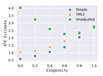
Figure 1: Adjusting for the network helps even when the no exogenous confounding assumption is violated. The robust TMLE estimator is the best estimator when no assumptions are violated. The simple conditional-outcome-only estimator (“Simple”) is better in the presence of moderate exogeneity. Plot shows estimates of ATE from district simulation. Ground truth is 1.

Comparison to baselines.

Table 1: Adjusting using the network improves ATE estimate in all cases. Further, the single-stage method is more accurate than baselines. Table entries are estimated ATE with 10-fold std. Ground truth is 1.0. Low and high confounding correspond to $\beta=1.0$ and $10.0$.

	age		district		join date
Conf.	Low	High	Low	High	Low	High
Unadjusted	$1.32$ p m 0.02	$4.34$ p m 0.05	$1.34$ p m 0.03	$4.51$ p m 0.05	$1.29$ p m 0.03	$4.03$ p m 0.06
Parametric	$1.30$ p m 0.00	$4.06$ p m 0.01	$1.21$ p m 0.00	$3.22$ p m 0.01	$1.26$ p m 0.00	$3.73$ p m 0.01
Two-stage	$1.33$ p m 0.02	$4.55$ p m 0.05	$1.34$ p m 0.02	$4.55$ p m 0.05	$1.30$ p m 0.03	$4.16$ p m 0.06
$\hat{\psi}^{\mathrm{A}}_{n}$	$1.24$ p m 0.04	$3.40$ p m 0.04	$1.09$ p m 0.02	$2.03$ p m 0.07	$1.21$ p m 0.05	$3.26$ p m 0.09

We report comparisons to the baselines in table 1. As expected, adjusting for the network improves estimation in every case. Further, the one-stage embedding procedure is more accurate than baselines.

Choice of estimator.

Table 2: The conditional-outcome-only estimator is usually most accurate. Table entries are estimated ATE with 10-fold std. Ground truth is 1.0. Low and high confounding correspond to $\beta=1.0$ and $10.0$.

	age		district		join date
Conf.	Low	High	Low	High	Low	High
$\hat{\psi}^{Q}_{n}$	$1.05$ p m 0.24	$2.77$ p m 0.35	$1.03$ p m 0.25	$1.75$ p m 0.20	$1.17$ p m 0.35	$2.41$ p m 0.45
$\hat{\psi}^{g}_{n}$	$1.27$ p m 0.03	$3.12$ p m 0.06	$1.10$ p m 0.03	$1.66$ p m 0.07	$1.29$ p m 0.05	$3.10$ p m 0.07
$\hat{\psi}^{\mathrm{A}}_{n}$	$1.24$ p m 0.04	$3.40$ p m 0.04	$1.09$ p m 0.02	$2.03$ p m 0.07	$1.21$ p m 0.05	$3.26$ p m 0.09
$\hat{\psi}^{\mathrm{TMLE}}_{n}$	$1.21$ p m 0.03	$3.26$ p m 0.07	$1.09$ p m 0.04	$2.02$ p m 0.05	$1.20$ p m 0.05	$3.13$ p m 0.09

We report comparisons of downstream estimators in table 2. The conditional-outcome-only estimator usually yields the best estimates, substantially improving on either robust method. This is likely because the network does not carry all information about the confounding factors, violating one of our assumptions. We expect that district has the strongest dependence with the network, and we see best performance for this attribute. Poor performance of robust estimators when assumptions are violated has been observed in other contexts [KS07].

Confounding exogenous to the network.  In practice, the network may not carry information about all sources of confounding. For instance, in our simulation, the confounders may not be wholly predictable from the network structure. We study the effect of exogenous confounding by a second simulation where the confounder consists of a part that can be fully inferred from the network and part that is wholly exogenous.

For the inferrable part, we use the estimated propensity scores $\{\hat{g}_{i}\}$ from the district experiment above. By construction, the network carries all information about each $\hat{g}_{i}$. We define the (ground truth) propensity score for our new simulation as $\operatorname*{logit}g_{\text{sim}}=(1-p)\operatorname*{logit}\hat{g}_{i}+p\xi_{i}$, with $\xi_{i}\overset{\mathrm{iid}}{\ \sim\ }\mathrm{N}(0,1)$. The second term, $\xi_{i}$, is the exogenous part of the confounding. The parameter $p$ controls the level of exogeneity. We simulate treatments and outcomes as in eq. 6.1.

In fig. 1 we plot the estimates at various levels of exogeneity. We observe that network adjustment helps even when the no exogenous confounding assumption is violated. Further, we see that the robust estimator has better performance when $p=0$, i.e., when the assumptions of Theorem 5.1 are satisfied. However, the conditional-outcome-only estimator is better if there is substantial exogenous confounding.

Appendix A Proof of Main Result

We now give the proof of Theorem 5.1, which establishes identifiability, consistency, and asymptotic normality.

Recall our setup:

• $Y$: outcome; $T$: treatment; $Z$: confounder.

• $Z$ is unobserved. We use some non-iid additional structure as a proxy.

• $(Y_{i},T_{i},Z_{i})\overset{\mathrm{iid}}{\ \sim\ }P$.

• $Q(t,z)=\mathbb{E}\left[Y\,|\,t,z\right]$; $g(Z)=P(T=1\,|\,Z)$

• The target parameter is the ATE,

  $$\psi_{0}=\mathbb{E}\left[Q(1,Z)-Q(0,Z)\right].$$

The estimator and the algorithm.  Recall that we learn the nuisance parameters $Q$, $g$, and the embeddings $\lambda$ using a semi-supervised embedding-based predictor. We allow a slightly more general construction of the estimator than in the body of the paper. In the body, we state the result only for the A-IPTW. Here, we allow any estimator that solves the efficient estimating equations. This allows, for example, for targeted minimum loss based estimation.

Step 1. Form a $K$-fold partition; the splits are $I_{k},k=1,\ldots,K$. For each set $I_{k}$, let $I^{c}_{k}$ denote the units not in $I_{k}$.

Construct $K$ estimators $\check{\psi}(I^{c}_{k}),k=1,\ldots,K$:

1. Estimate the nuisance parameters $Q$, $g$, and the embedding $\lambda$:

   $$\hat{\eta}(I^{c}_{k}):=\left(\hat{\lambda}_{i},\tilde{g}_{n}(\cdot;\hat{\gamma}^{g,I^{c}_{k}}_{n}),\tilde{Q}_{n}(\cdot,\cdot;\hat{\gamma}^{Q,I^{c}_{k}}_{n})\right)$$

2. $\check{\psi}(I^{c}_{k})$ is a solution to the following equation:

   $$\frac{1}{n_{K}}\sum_{i\in I_{k}}\varphi\left(Y_{i},T_{i},Z_{i};\psi_{0},\hat{\lambda}_{i},\tilde{g}_{n}(\cdot;\hat{\lambda}_{i},\hat{\gamma}^{g,I^{c}_{k}}_{n}),\tilde{Q}_{n}(\cdot,\cdot;\hat{\gamma}^{Q,I^{c}_{k}}_{n})\right)=0,$$

   where the $\varphi(\cdot)$ function is the efficient score:

   $$\varphi(Y,T,Z;\psi_{0},\lambda,\tilde{g}_{n},\tilde{Q}_{n})$$

   $$= \frac{T}{\tilde{g}_{n}(\lambda)}\{Y-\tilde{Q}_{n}(1,\lambda)\}-\frac{1-T}{1-\tilde{g}_{n}(\lambda)}\{Y-\tilde{Q}_{n}(0,\lambda)\}+\{\tilde{Q}_{n}(1,\lambda)-\tilde{Q}_{n}(0,\lambda)\}-\psi_{0}.$$

   We note that $\varphi$ does not depend on the unobserved $Z$.

Step 2. The final estimator for the ATE $\psi_{0}$ is

$$\tilde{\psi}=\frac{1}{K}\sum^{K}_{k=1}\check{\psi}(I^{c}_{k}).$$

The theorem and the proof.

See 1 See 2 See 3 See 4 See 5

Theorem A.1 (Validity).

Denote the true ATE as

$$\psi_{0}=\mathbb{E}_{P}\left[Q(1,Z)-Q(0,Z)\right].$$

Under Assumptions 1, 2, 3, 4 and 5 the estimator $\tilde{\psi}$ concentrates around $\psi_{0}$ with the rate $1/\sqrt{n}$ and is approximately unbiased and normally distributed:

$$\sigma^{-1}\sqrt{n}(\tilde{\psi}-\psi_{0})\stackrel{{\scriptstyle d}}{{\rightarrow}}\mathcal{N}(0,1)$$

$$\sigma^{2}=\mathbb{E}_{P}\left[\varphi^{2}_{0}\left(W;\psi_{0},\eta(\lambda(Z))\right)\right],$$

where

$$W =(Y,T,\lambda(Z)),$$

$$\eta(\lambda(Z)) =(g(\lambda(Z)),Q(T,\lambda(Z))),$$

and

$$\varphi_{0}(Y,T,\lambda(Z);\psi_{0},\eta(\lambda(Z)))$$

$$= \frac{T}{g(\lambda(Z))}\{Y-Q(1,\lambda(Z))\}-\frac{1-T}{1-g(\lambda(Z))}\{Y-Q(0,\lambda(Z))\}+\{Q(1,\lambda(Z))-Q(0,\lambda(Z))\}-\psi_{0}.$$

Proof.

We prove the result for the special case where $\lambda$ is the identity map. By Assumption 2 this is without loss of generality—it’s the case where all of the information in $Z$ is relevant for prediction. This is not an important mathematical point, but substantially simplifies notation.

The proof follow the same idea as in [Che+17a] with a few modifications accounting for the non-iid proxy structure.

We start with some notation.

1. $||\cdot||_{P,q}$ denotes the $L_{q}(P)$ norm. For example, for measurable $f:\mathcal{W}\stackrel{{\scriptstyle d}}{{\rightarrow}}\mathbb{R}$,

   $$||f(W)||_{P,q}:=(\int|f(w)^{q}\mathop{}\!\mathrm{d}P(w)|)^{1/q}.$$

2. The empirical process $\mathbb{G}_{n,I}(f(W))$ for $||f(W_{i})||_{P,2}<\infty$ is

   $$\mathbb{G}_{n,I}(f(W)):=\frac{1}{\sqrt{n}}\sum_{i\in I}(f(W_{i})-\int f(w)\mathop{}\!\mathrm{d}P(w)).$$

3. The empirical expectation and probability is

   $$\mathbb{E}_{n,I}\left[f(W)\right]:=\frac{1}{n}f(W_{i});\qquad\mathbb{P}_{n,I}(A):=\frac{1}{n}\sum_{i\in I}1(W_{i}\in A).$$

Let $\mathbb{P}_{n}$ be the empirical measure.

Step 1: (Main Step). Letting $\check{\psi}_{k}=\check{\psi}(I^{c}_{k})$, we first write

$$\sqrt{n}(\check{\psi}_{k}-\psi_{0})=\mathbb{G}_{n,I^{c}_{k}}\varphi(W;\psi_{0},\hat{\eta}(I^{c}_{k}))+\sqrt{n}\int\varphi(w;\psi_{0},\hat{\eta}(I^{c}_{k}))\mathop{}\!\mathrm{d}\mathbb{P}_{n}(w),$$ (A.1)

where

$$\hat{\eta}(I^{c}_{k}):=\left(\hat{\lambda}_{i},\tilde{g}_{n}(\cdot;\hat{\gamma}^{g,I^{c}_{k}}_{n}),\tilde{Q}_{n}(\cdot,\cdot;\hat{\gamma}^{Q,I^{c}_{k}}_{n})\right)$$

as is defined earlier.

Steps 2 and 3 below demonstrate that for each $k=1,\ldots,K$,

$$\int(\varphi(w;\psi_{0},\hat{\eta}(I^{c}_{k}))-\varphi_{0}(w;\psi_{0},\eta(z)))^{2}\mathop{}\!\mathrm{d}\mathbb{P}_{n}(w)=o_{\mathbb{P}_{n}}(1),$$ (A.2)

and that

$$\sqrt{n}\int\varphi(w;\psi_{0},\hat{\eta}(I^{c}_{k}))\mathop{}\!\mathrm{d}\mathbb{P}_{n}(w)=o_{\mathbb{P}_{n}}(1).$$ (A.3)

Equation A.2 implies

$$\mathbb{G}_{n,I^{c}_{k}}\left(\varphi(w;\psi_{0},\hat{\eta}(I^{c}_{k}))-\varphi_{0}(w;\psi_{0},\eta(z))\right)=o_{\mathbb{P}_{n}}(1)$$

due to Lemma B.1 of [Che+17a] and the Chebychev’s inequality.

We note that $\hat{\eta}(I^{c}_{k})=\left(\hat{\lambda}_{i},\tilde{g}_{n}(\cdot;\hat{\gamma}^{g,I^{c}_{k}}_{n}),\tilde{Q}_{n}(\cdot,\cdot;\hat{\gamma}^{Q,I^{c}_{k}}_{n})\right)$, where the embedding $\hat{\lambda}_{i}$’s are not independent. By contrast, $\eta(z)$ only depends on $Z_{i}$ where all $Z_{i}$’s are independent.

We next show $\sigma^{-1}\sqrt{n_{K}}(\check{\psi}_{k}-\psi_{0})_{k=1}^{K}=\sigma^{-1}\mathbb{G}_{n,I^{c}_{k}}\varphi_{0}(W;\psi_{0},\eta(Z))_{k=1}^{K}+o_{\mathbb{P}_{n}}(1)$.

First, we notice

$$\mathbb{E}\left[[\sqrt{n_{K}}(\check{\psi}_{k}-\psi_{0})-\mathbb{G}_{n,I^{c}_{k}}\varphi_{0}(W;\psi_{0},\eta(Z))]^{2}\,|\,I^{c}_{k}\right]$$

$$= \mathbb{E}\left[[\mathbb{G}_{n,I^{c}_{k}}\varphi(W;\psi_{0},\hat{\eta}(I^{c}_{k}))-\mathbb{G}_{n,I^{c}_{k}}\varphi_{0}(W;\psi_{0},\eta(Z))+o_{\mathbb{P}_{n}}(1)]^{2}\,|\,I^{c}_{k}\right]$$

$$= \mathbb{E}\left[(\mathbb{G}_{n,I^{c}_{k}}\varphi(W;\psi_{0},\hat{\eta}(I^{c}_{k})))^{2}\,|\,I^{c}_{k}\right]+\mathbb{E}\left[(\mathbb{G}_{n,I^{c}_{k}}\varphi_{0}(W;\psi_{0},\eta(Z)))^{2}\,|\,I^{c}_{k}\right]$$

$$-2\mathbb{E}\left[(\mathbb{G}_{n,I^{c}_{k}}\varphi(W;\psi_{0},\hat{\eta}(I^{c}_{k}))\cdot(\mathbb{G}_{n,I^{c}_{k}}\varphi_{0}(W;\psi_{0},\eta(Z)))\,|\,I^{c}_{k}\right]+o_{\mathbb{P}_{n}}(1)$$

The first equality is due to eq. A.1 and eq. A.2. The second equality is due to

$$\mathbb{E}\left[\mathbb{G}_{n,I^{c}_{k}}\varphi(W;\psi_{0},\hat{\eta}(I^{c}_{k}))\right]=\mathbb{E}\left[\mathbb{G}_{n,I^{c}_{k}}\varphi_{0}(W;\psi_{0},\eta(Z))\right]=0.$$ (A.4)

If we write $\bar{\varphi}(W_{i}):=\varphi(W_{i})-\int\varphi(w)\mathop{}\!\mathrm{d}\mathbb{P}_{n}(w)$, we have

$$\mathbb{E}\left[[\sqrt{n_{K}}(\check{\psi}_{k}-\psi_{0})-\mathbb{G}_{n,I^{c}_{k}}\varphi_{0}(W;\psi_{0},\eta(Z))]^{2}\,|\,I^{c}_{k}\right]$$

$$= \frac{1}{n}\mathbb{E}\left[\sum_{i,j=1}^{n_{K}}\bar{\varphi}(W_{i};\psi_{0},\hat{\eta}(I^{c}_{k}))\cdot\bar{\varphi}(W_{j};\psi_{0},{\eta}(I^{c}_{k}))\,|\,I^{c}_{k}\right]$$

$$+\frac{1}{n}\mathbb{E}\left[\sum_{i,j=1}^{n_{K}}\bar{\varphi}_{0}(W_{i};\psi_{0},{\eta}(Z_{i}))\cdot\bar{\varphi}_{0}(W_{j};\psi_{0},\hat{\eta}(Z_{j}))\right]$$

$$-2\mathbb{E}\left[(\mathbb{G}_{n,I^{c}_{k}}\varphi(W;\psi_{0},\hat{\eta}(I^{c}_{k}))\,|\,I^{c}_{k}\right]\cdot\mathbb{E}\left[(\mathbb{G}_{n,I^{c}_{k}}\varphi_{0}(W;\psi_{0},\eta(Z)))\right]+o_{\mathbb{P}_{n}}(1)$$

$$= \frac{1}{n}\sum_{i,j=1}^{n_{K}}o(\frac{1}{n})+\frac{1}{n}\sum_{i,j=1}^{n_{K}}\mathbb{E}\left[\bar{\varphi}_{0}(W_{i};\psi_{0},{\eta}(Z_{i}))\right]\cdot\mathbb{E}\left[\bar{\varphi}_{0}(W_{j};\psi_{0},\hat{\eta}(Z_{j}))\right]+o_{\mathbb{P}_{n}}(1)$$

$$= o_{\mathbb{P}_{n}}(1)$$

The second equality is due to Assumption 5, the independence of $W_{i}$’s, and Equation A.4.

By Lemma B.1 of [Che+17a],

$$\mathbb{E}\left[[\sqrt{n_{K}}(\check{\psi}_{k}-\psi_{0})-\mathbb{G}_{n,I^{c}_{k}}\varphi_{0}(W;\psi_{0},\eta(Z))]^{2}\,|\,I^{c}_{k}\right]=o_{\mathbb{P}_{n}}(1)$$

implies

$$\sqrt{n_{K}}(\check{\psi}_{k}-\psi_{0})-\mathbb{G}_{n,I^{c}_{k}}\varphi_{0}(W;\psi_{0},\eta(Z))=o_{\mathbb{P}_{n}}(1)$$

Therefore, we have

$$\sigma^{-1}\sqrt{n_{K}}(\check{\psi}_{k}-\psi_{0})_{k=1}^{K}=\sigma^{-1}\mathbb{G}_{n,I^{c}_{k}}\varphi_{0}(W;\psi_{0},\eta(Z))_{k=1}^{K}+o_{\mathbb{P}_{n}}(1)\stackrel{{\scriptstyle d}}{{\rightarrow}}(\mathcal{N}_{k})_{k=1}^{K}$$

where $(\mathcal{N}_{k})_{k=1}^{K}$ is a Gaussian vector with independent $\mathcal{N}(0,1)$ coordinates. Using the independence of $Z_{i}$’s and the central limit theorem, we have

$$\sigma^{-1}\sqrt{n}(\tilde{\psi}-\psi_{0})$$

$$= \sigma^{-1}\sqrt{n}(\frac{1}{K}\sum^{K}_{k=1}(\check{\psi}_{k}-\psi_{0}))$$

$$= \frac{1}{K}\sigma^{-1}\sum^{K}_{k=1}\mathbb{G}_{n,I^{c}_{k}}\varphi_{0}(W;\psi_{0},\eta(Z))+o_{\mathbb{P}_{n}}(1)$$

$$\stackrel{{\scriptstyle d}}{{\rightarrow}} \frac{1}{K}\sum^{K}_{k=1}\mathcal{N}_{k}=\mathcal{N}(0,1).$$

Step 2: This step demonstrates Equation A.2. Observe that for some constant $C_{\varepsilon}$ that depends only on $\varepsilon$ and $\mathcal{P}$,

$$||\varphi(W;\psi_{0},\hat{\eta}(I^{c}_{k}))-\varphi(W;\psi_{0},\eta(Z))||_{\mathbb{P}_{n},2}\leq C_{\varepsilon}(\mathcal{I}_{1}+\mathcal{I}_{2}+\mathcal{I}_{3}),$$

where

$$\mathcal{I}_{1} =\max_{d\in\{0,1\}}||\tilde{Q}_{n}(d,Z;\hat{\gamma}^{Q,I^{c}_{k}}_{n})-Q(d,Z)||_{\mathbb{P}_{n},2},$$

$$\mathcal{I}_{2} =||\frac{T(Y-\tilde{Q}_{n}(1,\lambda;\hat{\gamma}^{Q,I^{c}_{k}}_{n}))}{\tilde{g}_{n}(\cdot;\hat{\gamma}^{g,I^{c}_{k}}_{n})}-\frac{T(Y-Q(1,Z))}{g(\lambda)}||_{\mathbb{P}_{n},2},$$

$$\mathcal{I}_{3} =||\frac{(1-T)(Y-\tilde{Q}_{n}(0,\lambda;\hat{\gamma}^{Q,I^{c}_{k}}_{n}))}{1-\tilde{g}_{n}(\cdot;\hat{\gamma}^{g,I^{c}_{k}}_{n})}-\frac{(1-T)(Y-Q(0,Z))}{1-g(\lambda)}||_{\mathbb{P}_{n},2},$$

We bound $\mathcal{I}_{1},\mathcal{I}_{2},\text{ and }\mathcal{I}_{3}$ in turn. First, $\mathbb{P}_{n}(\mathcal{I}_{1}>\delta_{n_{K}})\leq\Delta_{n_{K}}\rightarrow 0$ by Assumption 4, and so $\mathcal{I}_{1}=o_{\mathbb{P}_{n}}(1)$. Also, on the event that

$$\mathbb{P}_{n}(\varepsilon\leq\tilde{g}_{n}(Z;I^{c}_{k})\leq 1-\varepsilon)=1$$ (A.5)

$$||\tilde{Q}_{n}(1,\lambda;\hat{\gamma}^{Q,I^{c}_{k}}_{n})-Q(1,Z)||_{\mathbb{P}_{n},2}+||\tilde{g}_{n}(\cdot;\hat{\gamma}^{g,I^{c}_{k}}_{n})-g(Z)||_{\mathbb{P}_{n},2}\leq\delta_{n_{K}},$$ (A.6)

which happens with $P_{\mathbb{P}_{n}}$-probability at least $1-\Delta_{n_{K}}$ by Assumption 4,

$$\mathcal{I}_{2} \leq\varepsilon^{-2}||Tg(Z)(Y-\tilde{Q}_{n}(1,\lambda;\hat{\gamma}^{Q,I^{c}_{k}}_{n}))-T\tilde{g}_{n}(Z;I^{c}_{k})(Y-Q(1,Z))||_{\mathbb{P}_{n},2}$$

$$\leq\varepsilon^{-2}||g(Z)(Q(1,Z)+\zeta-\tilde{Q}_{n}(1,\lambda;\hat{\gamma}^{Q,I^{c}_{k}}_{n}))-\tilde{g}_{n}(Z;I^{c}_{k})\zeta||_{\mathbb{P}_{n},2}$$

$$\leq\varepsilon^{-2}||g(Z)(\tilde{Q}_{n}(1,\lambda;\hat{\gamma}^{Q,I^{c}_{k}}_{n})-Q(1,Z))||_{\mathbb{P}_{n},2}+||(\tilde{g}_{n}(Z;I^{c}_{k})-g(Z))\zeta||_{\mathbb{P}_{n},2}$$

$$\leq\varepsilon^{-2}||\tilde{Q}_{n}(1,\lambda;\hat{\gamma}^{Q,I^{c}_{k}}_{n})-Q(1,Z)||_{\mathbb{P}_{n},2}+\sqrt{C}||\tilde{g}_{n}(Z;I^{c}_{k})-g(Z)||_{\mathbb{P}_{n},2}$$

$$\leq\varepsilon^{-2}(\delta_{n_{K}}+\sqrt{C}\delta_{n_{K}})\rightarrow 0,$$

where the first inequality follows from Equation A.5 and Assumption 4, the second from the facts that $T\in\{0,1\}$ and for $T=1,Y=Q(1,Z)+\zeta$, the third from the triangle inequality, the fourth from the facts that $\mathbb{P}_{n}(g(Z)\leq 1)=1$ and $\mathbb{P}_{n}(\mathbb{E}_{\mathbb{P}_{n}}\left[\zeta^{2}\,|\,Z\right]\leq C)=1$ in Assumption 3, the fifth from Equation A.6, and the last assertion follows since $\delta_{n_{K}}\rightarrow 0$. Hence, $\mathcal{I}_{2}=o_{\mathbb{P}_{n}}(1)$. In addition, the same argument shows that $\mathcal{I}_{3}=o_{\mathbb{P}_{n}}(1)$, and so Equation A.2 follows.

Step 3: This step demonstrates Equation A.3. Observe that since $\psi_{0}=\mathbb{E}_{\mathbb{P}_{n}}\left[Q(1,Z)-Q(0,Z)\right]$, the left-hand side of Equation A.3 is equal to

$$\mathcal{I}_{4}= \sqrt{n}\int\frac{\tilde{g}_{n}(Z;I^{c}_{k})-g(z)}{\tilde{g}_{n}(Z;I^{c}_{k})}\cdot(\tilde{Q}_{n}(1,\lambda;\hat{\gamma}^{Q,I^{c}_{k}}_{n})-Q(1,z))$$

$$+\frac{\tilde{g}_{n}(Z;I^{c}_{k})-g(z)}{1-\tilde{g}_{n}(Z;I^{c}_{k})}\cdot(Q(0,z;I^{c}_{k})-Q(0,z))\mathop{}\!\mathrm{d}\mathbb{P}_{n}(z).$$

But on the event that

$$\mathbb{P}_{n}(\varepsilon\leq\tilde{g}_{n}(Z;I^{c}_{k})\leq 1-\varepsilon)=1$$

and

$$\max_{d\in\{0,1\}}||\tilde{Q}_{n}(d,\lambda;\hat{\gamma}^{Q,I^{c}_{k}}_{n})-Q(d,Z)||_{\mathbb{P}_{n},2}\cdot||\tilde{g}_{n}(Z;I^{c}_{k})-g(Z)||_{\mathbb{P}_{n},2}\leq\delta_{n_{K}}\cdot n_{K}^{-1/2},$$

which happens with $P_{\mathbb{P}_{n}}$-probability at least $1-\Delta_{n_{K}}$ by Assumption 4,the Cauchy-Schwarz inequality implies that

$$\mathcal{I}_{4}\leq\frac{2\sqrt{n}}{\varepsilon}\max_{d\in\{0,1\}}||\tilde{Q}_{n}(d,\lambda;\hat{\gamma}^{Q,I^{c}_{k}}_{n})-Q(d,Z)||_{\mathbb{P}_{n},2}\cdot||\tilde{g}_{n}(Z;I^{c}_{k})-g(Z)||_{\mathbb{P}_{n},2}\leq\frac{2\delta_{n_{K}}}{\varepsilon}\rightarrow 0,$$

which gives Equation A.3.

∎

References

• [Air+08] E. Airoldi, D. Blei, S. Fienberg and E. Xing β€œMixed Membership Stochastic Blockmodels” In Journal of Machine Learning Research 9, 2008, pp. 1981–2014
• [Bic+00] P. J. Bickel, C. A. J. Klaassen, Y. Ritov and J. A. Wellner β€œEfficient and Adaptive Estimation for Semiparametric Models” In Sankhyā: The Indian Journal of Statistics, Series A 62, 2000, pp. 157–160 DOI: 10.2307/25051300
• [Cha+17] Benjamin Paul Chamberlain, James Clough and Marc Peter Deisenroth β€œNeural Embeddings of Graphs in Hyperbolic Space” In arXiv e-prints, 2017, pp. arXiv:1705.10359 arXiv:1705.10359 [stat.ML]
• [Che+17] Victor Chernozhukov et al. β€œDouble/Debiased Machine Learning for Treatment and Structural parameters” In The Econometrics Journal Wiley Online Library, 2017
• [Che+17a] Victor Chernozhukov et al. β€œDouble/Debiased/Neyman Machine Learning of Treatment Effects” In American Economic Review 107.5, 2017, pp. 261–65 DOI: 10.1257/aer.p20171038
• [CH08] Stephen R Cole and Miguel A. HernΓ‘n β€œConstructing inverse probability weights for marginal structural models.” In American Journal of Epidemiology 168 6, 2008, pp. 656–64
• [CD15] Harry Crane and Walter Dempsey β€œA framework for statistical network modeling” In arXiv e-prints, 2015, pp. arXiv:1509.08185 arXiv:1509.08185 [math.ST]
• [Dur06] R. Durrett β€œRandom Graph Dynamics” Cambridge University Press, 2006
• [GB13] Prem K. Gopalan and David M. Blei β€œEfficient discovery of overlapping communities in massive networks” In Proceedings of the National Academy of Sciences National Academy of Sciences, 2013 DOI: 10.1073/pnas.1221839110
• [Ham+17] Will Hamilton, Zhitao Ying and Jure Leskovec β€œInductive Representation Learning on Large Graphs” In Advances in Neural Information Processing Systems 30 Curran Associates, Inc., 2017, pp. 1024–1034 URL: http://papers.nips.cc/paper/6703-inductive-representation-learning-on-large-graphs.pdf
• [Ham+17a] William L. Hamilton, Rex Ying and Jure Leskovec β€œRepresentation Learning on Graphs: Methods and Applications” In arXiv e-prints, 2017, pp. arXiv:1709.05584 arXiv:1709.05584 [cs.SI]
• [Hof+02] P. Hoff, A. Raftery and M. Handcock β€œLatent space approaches to social network analysis” In Journal of the American Statistical Association 97.460, 2002, pp. 1090–1098
• [KS07] Joseph D. Y. Kang and Joseph L. Schafer β€œDemystifying double robustness: a comparison of alternative strategies for estimating a population mean from incomplete data” In Statist. Sci. 22.4, 2007, pp. 523–539 DOI: 10.1214/07-STS227
• [KM99] Manabu Kuroki and Masami Miyakawa β€œIDENTIFIABILITY CRITERIA FOR CAUSAL EFFECTS OF JOINT INTERVENTIONS” In Journal of the Japan Statistical Society 29.2, 1999, pp. 105–117 DOI: 10.14490/jjss1995.29.105
• [KP14] Manabu Kuroki and Judea Pearl β€œMeasurement bias and effect restoration in causal inference” In Biometrika 101.2, 2014, pp. 423–437 DOI: 10.1093/biomet/ast066
• [LK14] Jure Leskovec and Andrej Krevl β€œSNAP Datasets: Stanford Large Network Dataset Collection”, http://snap.stanford.edu/data, 2014
• [Lou+17] Christos Louizos et al. β€œCausal effect inference with deep latent-variable models” In Advances in Neural Information Processing Systems, 2017, pp. 6449–6459
• [Mia+18] Wang Miao, Zhi Geng and Eric J Tchetgen Tchetgen β€œIdentifying causal effects with proxy variables of an unmeasured confounder” In Biometrika 105.4, 2018, pp. 987–993 DOI: 10.1093/biomet/asy038
• [New09] M. Newman β€œNetworks. An Introduction” Oxford University Press, 2009
• [Ogb18] Elizabeth L. Ogburn β€œChallenges to Estimating Contagion Effects from Observational Data” In Complex Spreading Phenomena in Social Systems: Influence and Contagion in Real-World Social Networks Cham: Springer International Publishing, 2018, pp. 47–64 DOI: 10.1007/978-3-319-77332-2_3
• [OV17] Elizabeth L. Ogburn and Tyler J. VanderWeele β€œVaccines, contagion, and social networks” In Ann. Appl. Stat. 11.2 The Institute of Mathematical Statistics, 2017, pp. 919–948 DOI: 10.1214/17-AOAS1023
• [Ogb+17] Elizabeth L. Ogburn, Oleg Sofrygin, Ivan Diaz and Mark J. van der Laan β€œCausal inference for social network data” In arXiv e-prints, 2017, pp. arXiv:1705.08527 arXiv:1705.08527 [stat.ME]
• [OR15] P. Orbanz and D.M. Roy β€œBayesian Models of Graphs, Arrays and Other Exchangeable Random Structures” In Pattern Analysis and Machine Intelligence, IEEE Transactions on 37.2, 2015, pp. 437–461 DOI: 10.1109/TPAMI.2014.2334607
• [Pea12] Judea Pearl β€œOn Measurement Bias in Causal Inference” In arXiv e-prints, 2012, pp. arXiv:1203.3504 arXiv:1203.3504 [stat.ME]
• [Per+14] Bryan Perozzi, Rami Al-Rfou and Steven Skiena β€œDeepWalk: Online Learning of Social Representations” In Proc.Β 20th Int.Β Conference on Knowledge Discovery and Data Mining (KDD ’14) ACM, 2014, pp. 701–710 URL: http://doi.acm.org/10.1145/2623330.2623732
• [Rob00] J. M. Robins β€œRobust Estimation in Sequentially Ignorable Missing Data and Causal Inference Models” In ASA Proceedings of the Section on Bayesian Statistical Science 1999, 2000
• [Rob+94] James M. Robins, Andrea Rotnitzky and Lue Ping Zhao β€œEstimation of Regression Coefficients When Some Regressors are not Always Observed” In Journal of the American Statistical Association 89.427 Taylor & Francis, 1994, pp. 846–866 DOI: 10.1080/01621459.1994.10476818
• [Rob+00] James M. Robins, Andrea Rotnitzky and Mark Laan β€œOn Profile Likelihood: Comment” In Journal of the American Statistical Association 95.450 [American Statistical Association, Taylor & Francis, Ltd.], 2000, pp. 477–482 URL: http://www.jstor.org/stable/2669391
• [RR83] Paul R. Rosenbaum and Donal B. Rubin β€œThe central role of the propensity score in observational studies for causal effects” In Biometrika 70.1, 1983, pp. 41–55 DOI: 10.1093/biomet/70.1.41
• [SM16] Cosma Shalizi and Edward McFowland III β€œEstimating Causal Peer Influence in Homophilous Social Networks by Inferring Latent Locations” In arXiv e-prints, 2016, pp. arXiv:1607.06565 arXiv:1607.06565 [stat.ME]
• [ST11] Cosma Rohilla Shalizi and Andrew C. Thomas β€œHomophily and contagion are generically confounded in observational social network studies” In Sociol. Methods Res. 40.2, 2011, pp. 211–239 DOI: 10.1177/0049124111404820
• [TZ12] Lubos Takac and Michal Zabovsky β€œDATA ANALYSIS IN PUBLIC SOCIAL NETWORKS” In International Scientific Conference and International Workshop Present Day Trends of Innovations, 2012 URL: https://snap.stanford.edu/data/soc-Pokec.html
• [Tch+17] Eric J. Tchetgen Tchetgen, Isabel Fulcher and Ilya Shpitser β€œAuto-G-Computation of Causal Effects on a Network” In arXiv e-prints, 2017, pp. arXiv:1709.01577 arXiv:1709.01577 [stat.ME]
• [vR11] Mark van der Laan and Sherri Rose β€œTargeted Learning: Causal Inference for Observational and Experimental Data”, 2011 DOI: 10.1007/978-1-4419-9782-1
• [VR15] Victor Veitch and Daniel M. Roy β€œThe Class of Random Graphs Arising from Exchangeable Random Measures” In arXiv e-prints, 2015, pp. arXiv:1512.03099 arXiv:1512.03099 [math.ST]
• [Vei+19] Victor Veitch et al. β€œEmpirical Risk Minimization and Stochastic Gradient Descent for Relational Data” In Proceedings of the 22nd International Conference on Artificial Intelligence and Statistics, 2019
• [Vei+19a] Victor Veitch, Dhanya Sridhar and David M. Blei β€œUsing Text Embeddings for Causal Inference” In arXiv e-prints, 2019, pp. arXiv:1905.12741 arXiv:1905.12741 [cs.LG]
• [WW87] Y. Wang and G. Wong β€œStochastic Block Models for Directed Graphs” In Journal of the American Statistical Association 82.397, 1987, pp. 8–19
• [Yan+16] Zhilin Yang, William Cohen and Ruslan Salakhudinov β€œRevisiting Semi-Supervised Learning with Graph Embeddings” In Proceedings of The 33rd International Conference on Machine Learning 48 New York, New York, USA: PMLR, 2016, pp. 40–48 URL: http://proceedings.mlr.press/v48/yanga16.html