Stellar Activity Effects on Moist Habitable Terrestrial Atmospheres Around M dwarfs

Abstract

Transit spectroscopy of terrestrial planets around nearby M dwarfs is a primary goal of space missions in coming decades. 3-D climate modeling has shown that slow-synchronous rotating terrestrial planets may develop thick clouds at the substellar point, increasing the albedo. For M dwarfs with $T$eff > 3000 K, such planets at the inner habitable zone (IHZ) have been shown to retain moist greenhouse conditions, with enhanced stratospheric water vapor ($fH_{2}O$ > 10^-3) and low Earth-like surface temperatures. However, M dwarfs also possess strong UV activity, which may effectively photolyze stratospheric H₂O. Prior modeling efforts have not included the impact of high stellar UV activity on the H₂O. Here, we employ a 1-D photochemical model with varied stellar UV, to assess whether H₂O destruction driven by high stellar UV would affect its detectability in transmission spectroscopy. Temperature and water vapor profiles are taken from published 3-D climate model simulations for an IHZ Earth-sized planet around a 3300 K M dwarf with an N₂-H₂O atmosphere; they serve as self-consistent input profiles for the 1-D model. We explore additional chemical complexity within the 1-D model by introducing other species into the atmosphere. We find that as long as the atmosphere is well-mixed up to 1 mbar, UV activity appears to not impact detectability of H₂O in the transmission spectrum. The strongest H₂O features occur in the JWST MIRI instrument wavelength range and are comparable to the estimated systematic noise floor of ~50 ppm.

1 Introduction

Planets orbiting close enough to their host M dwarf stars to be tidally-locked have their day-sides continuously subjected to the enormous UV stellar irradiation. The first habitable zone (HZ) exoplanets to have their atmospheres characterized will likely be such tidally-locked planets orbiting nearby M dwarf stars. Thus there is a need to understand the behavior of such planetary atmospheres. Observed spectroscopic signatures from transit measurements can reveal spectrally active species in a planet’s atmosphere. Present observational technologies not only inform us about the observed atmosphere’s composition, but can also shed light on the planet’s physical properties and atmospheric dynamics. NASA’s upcoming space missions, such as the James Webb Space Telescope (JWST), will meet the sensitivity and broad wavelength coverage requirements to constrain extrasolar planetary atmospheric composition with unprecedented accuracy.

Chemical disequilibrium processes (e.g. photolysis, vertical convection, life, etc.) can be diagnosed in planetary atmospheres by studying the observed trends in the abundances of detected species (e.g. Line & Yung 2013). In the deep atmosphere, where pressures and temperatures are high, reaction timescales are short. So, species tend to stay in chemical equilibrium. Temperatures tend to decrease with increasing altitude in planetary atmospheres without thermal inversions, slowing the reaction rates to a point where vertical transport starts dominating, causing species to spread out. For slowly rotating Earth-like planets, changes to the large-scale circulation lead to an increased efficiency of vertical mixing (Yang et al., 2013). This means the lower unobserved region–the troposphere–is able to communicate with the upper regions probed by our space infra-red (IR) instruments. In the uppermost regions, the high ultra-violet (UV) instellation (i.e. stellar insolation from stars other than the Sun) can lead to photolysis and increasing depletion in the abundances of some molecular species. Planets with equilibrium temperatures below 1200K (i.e. they receive < 340-400 times the Earth-equivalent instellation S_o, using geometric albedo range 0.01-0.15 from Heng & Demory (2013)), have been shown to have the most obvious signs of disequilibrium via chemical kinetics modeling (Liang et al., 2003, 2004; Zahnle et al., 2009b, a; Line & Yung, 2013; Moses et al., 2011, 2013; Visscher & Moses, 2011; Kopparapu et al., 2012; Hu et al., 2012; Miller-Ricci Kempton et al., 2012).

Disequilibrium mechanisms play a noticeable role in altering atmospheric composition at altitudes probed by remote sensing techniques. Disequilibrium sources within the solar system include Venus’s sulfuric acid hazes (e.g. Yung & Demore 1982; Krasnopolsky & Pollack 1994), Titan’s hydrocarbon hazes (e.g. Allen et al. 1980; Yung et al. 1984, and even Earth’s ozone–a product of O₂ photolysis (e.g. Chapman 1930a, b, 1942. Observational (Knutson et al., 2014; Kreidberg et al., 2014, 2018; Greene et al., 2016; Wakeford et al., 2015, 2017) and theoretical (Benneke & Seager, 2013; Mbarek & Kempton, 2016; Arney et al., 2017; Heng & Demory, 2013; Morley et al., 2017) studies have shown that clouds and hazes dominate both transmission and reflection spectra of all kinds of planets. They can alter the thermal structure and composition in the higher altitudes, in addition to masking spectral features from the lower atmosphere. 3-D climate simulations have shown that for synchronously rotating planets, persistent substellar clouds may act in favor of habitability by increasing planetary albedo and decreasing the surface temperature, allowing planets to remain habitable at higher stellar fluxes than that of Earth’s (e.g. Yang et al. 2013; Way et al. 2016; Kopparapu et al. 2016, 2017; Bin et al. 2018). A synchronous orbit around the host star is a valid assumption for planets in the habitable zones of such low mass stars (Leconte et al., 2015).

Planet rotation rate, and thus the Coriolis effect, plays a key role in modulating atmospheric circulation and climate (e.g. Merlis & Schneider 2010; Yang et al. 2014a; Noda et al. 2017; Fujii et al. 2018). For slowly rotating planets, the Coriolis effect is weak, and planets maintain large-scale day-night thermal circulation patterns. Such worlds are characterized by strong convection and upwelling air around their substellar point, and downwelling air on the antistellar side. These effects combine to yield strong vertical mixing of H₂O, which creates the ubiquitous subtellar cloud deck for slow rotators (e.g. Yang et al. 2013), and significantly enhances stratospheric H₂O planet-wide (Kopparapu et al., 2017; Fujii et al., 2017). Planetary stratospheres are more readily sensed by transit observations than tropospheres due to refraction effects (e.g. Misra et al. 2014, Bétrémieux & Kaltenegger 2015), and cloud opacity can prohibit observations of the relatively wet lower layers. The exact range of pressures accessible to and sensed by IR observations depends on the star-planet distance as well as the star and planet type, since the location of condensates vary with those parameters. Kopparapu et al. (2017) found that slow rotators around M dwarfs maintain moist-greenhouse conditions (stratospheric H₂O content >10^-3, Kasting et al. 1993), despite relatively mild surface temperatures (~280 K). Therefore, we may expect to observe stronger H₂O features in the transmission spectra of habitable slow rotators around M dwarfs compared to a true Earth-twin; Earth has a relatively dry stratosphere (fH₂O~10^-6). At 1 mbar (the model top of the 3-D climate model), vertical mixing should remain strong enough to compete with the photochemical H₂O loss (Yang et al., 2014a; Kopparapu et al., 2016; Fujii et al., 2017). The question then becomes, is the H₂O loss above 1 mbar from photodisassociation significant enough to affect our ability to detect it with JWST? If so, can we quantify this effect?

To answer this, we study the composition of such planets with a 1-D atmospheric model that includes chemical kinetics (including photolysis) and vertical mixing. We explore the influence of UV irradiation on the composition of the atmosphere at the planet’s terminator (simulated by a 3-D climate model), which is probed by transit transmission observations. We consider a 1-D model column extending above the stratosphere to explore chemical complexity from photochemical disequilibrium and its impact on observing. We look for any discernible impact on the spectra of a selected planet-star pair within the moist greenhouse regime of Kopparapu et al. (2017). Here we report our findings for an N₂-H₂O-dominated moist terrestrial IHZ planet modeled around a 3300 K M dwarf with synthetically varied stellar UV emissions from 1216 Å - 4000 Å. We compare our spectra with Kopparapu et al. (2017) and discuss implications for future observations of moist habitable atmospheres with JWST.

The rest of this paper is laid out as follows: In Section 2, we give an overview of the analysis method and describe the various modeling tools employed in this study. In Section 3, we present our findings for each stellar profile scenario, for a total of five scenarios. In Section 4, we discuss the implications of the results on molecular detection via future observations with JWST, and we conclude in Section 5.

2 Methods

We use 3-D global climate model (GCM) results of a specific H₂O-rich atmosphere case from Kopparapu et al. (2017) as the input for our 1-D models in this study (see Table 1, more details in Section 2.1). Specifically, we use terminator mean vertical profiles of P, T, N₂ and H₂O from the GCM as inputs for a 1-D photochemistry model. We augment our 1-D atmospheres with other species (see Section 2.3), including a "modern Earth" constant CO₂ mixing ratio of 360 ppm. We let the atmosphere evolve for five different UV cases (see Section 2.2), including the original UV-quiet model star used in the Kopparapu et al. (2017) study. We determine steady state abundances for all modeled species for each simulated atmosphere. We then generate transmission spectra to determine the spectral observables of these habitable moist greenhouse atmospheres with self-consistent photochemistry.

Table 1: 1-D Model Parameters: Planet and Star Properties

Parameter	Value
Planet Mass	1$M_{\oplus}$
Planet Radius	1$R_{\oplus}$
Planet Surface Gravity	1g
Planet Surface Pressure	1.008 bar
Planet Surface Temperature	266 K
Star Radius	0.137$R_{\odot}$
Star Temperature Teff	3300 K (Spectral Type M3)
Star Insolation Flux	1650 W/m2 (1.21So)

The 3-D and 1-D models are not coupled–the GCM is run first and the output fed to the photochemical model, but the output from the latter does not provide feedback into the GCM. Currently, there is no 3-D model available with full chemical mapping capabilities for planets around M dwarfs. GCMs also do not extend to very low pressures, and thus cannot fully capture dynamics affecting upper atmosphere composition. The GCM is the Community Atmosphere Model (CAM), developed by the National Center for Atmospheric Research (NCAR) to simulate the climate of Earth (Neale et al., 2010). For the Kopparapu et al. (2017) work, Version 4 (CAM4) was adapted to simulate Earth-like aquaplanets (i.e. an ocean planet with no land) around M dwarf stars. For our 1-D chemical modeling, we use the Atmos 1-D photochemical modeling tool, most recently developed by the Virtual Planetary Laboratory (VPL). Atmos comes with stellar flux data from the VPL spectral database. We use this data and stellar spectra from the MUSCLES Treasury Survey (Youngblood et al., 2016) to provide a range of UV fluxes for the UV-active simulations. This way we are able to realistically portray time-averaged low, medium, and high UV activity. We run a single 1-D model per UV case, for a total of five UV cases (Inactive/Low UV, Medium UV 1, Medium UV 2, High UV, Very High UV). We thus run five photochemical models for the same planet (see Table 1), each initiated with same physical properties and mixing ratio profiles. We use the Exo-Transmit spectral tool to compute the transmission spectrum for each UV model (Kempton et al., 2017).

2.1 Planet Parameters: Moist Atmosphere Simulations

CAM has been widely used for studies of habitable exoplanets (Yang et al., 2013, 2014a, 2016; Shields et al., 2013; Yang et al., 2014b; Wolf & Toon, 2014, 2015; Kopparapu et al., 2016, 2017; Wolf, 2017; Haqq-Misra et al., 2018; Wang et al., 2014, 2016; Bin et al., 2018). CAM4 has been updated to include a flexible correlated-k radiative transfer module (Wolf & Toon, 2013), and updated water-vapor absorption coefficients from HITRAN2012. The moist habitable atmospheres computed by CAM4 Kopparapu et al. (2017) assumed an Earth mass aquaplanet, with a 50m thick "slab" ocean. The slab ocean acts as a thermodynamic layer, where energy fluxes (radiant, latent, and sensible) are calculated between atmosphere and ocean. There is no ocean heat transport, thus the temperature of the ocean is set by surface energy exchange process only. All simulations assumed an atmosphere composed of 1 bar of N₂ and variable H₂O. Further details on the numerical scheme can be found in Neale et al. (2010) and Section 2.1 of Kopparapu et al. (2017).

We use the terminator mean surface values and vertical profiles from a single GCM run from Kopparapu et al. (2017) as the inputs for our 1-D models here. We use the planetary terminator results of the 3300 K model star irradiating the synchronously rotating (orbital-rotational period: 19.5724 days) Earth-like planet (see Table 1) at 1650 W/m² (1.21S_o).

In Kopparapu et al. (2017), GCM simulations were conducted for HZ planets around six different M dwarf model stars (T_eff = 2600 K, 3000 K 3300 K, 3700 K, 4000 K, 4500 K). The study focused on climate states near the inner edge of the HZ, the runaway greenhouse effect, and stratospheric H₂O. Thus the model planets were subject to increasing stellar fluxes until a runaway greenhouse was triggered, marking the terminal inner edge of the HZ. The runaway greenhouse effect is characterized by a collapse of the substellar cloud deck, and a sharp reduction in the planet’s albedo. Temperatures rise rapidly, as a large top of atmosphere (TOA) energy imbalance is maintained, and the increasingly strong water vapor greenhouse prevents the planet from radiatively cooling (e.g. Figures 6 and 7 from Kopparapu et al. (2017)).

For planets orbiting M dwarf stars with T_eff $\leq$ 3000 K, atmospheres transitioned from mild climates with little stratospheric water vapor directly to a runaway greenhouse, with no stable moist greenhouse state existing between (but see Bin et al. (2018)). For stars with T_eff $\geq$ 3300 K, Kopparapu et al. (2017) found that the planets can maintain a stable moist greenhouse regime with their climate remaining stable against a runaway greenhouse. For our study here, we choose a stable moist greenhouse state around a 3300 K star. Detections around a 3300 K star will be easier than those around larger hosts because a smaller star means larger transit signals, and a shorter orbital period means that more transit observations can be stacked together in a shorter period of time, improving signal to noise. The 3300 K star was thereby the sole case for which spectra were shown and implications for MIRI observations discussed in Kopparapu et al. (2017). So we are able to compare to those results directly in Section 4.

Our input P-T profile (i.e. mean terminator thermal profile from the GCM) shows a temperature minimum at 2 mbar, which translates to a cold trap in the H₂O profile where cloud condensation would occur. Table 1 of Kopparapu et al. (2017) reports a GCM model top H₂O mixing ratio of 5.55x10^-4. While this is the global mean value across stratosphere, the mean terminator value is similar due to the strong mixing. Since photolysis of water vapor increases with altitude due to the strengthening incoming stellar UV, we also want to explore the region above 1 mbar in this study. Thus we extend the 1 mbar H₂O and $T(P)$ values to a TOA pressure of 8.1x10^-7 bar in our 1-D simulations by simply holding them constant at those values for the atmosphere above 1 mbar in the input profile; photochemical kinetics drives the ultimate steady state abundances.

2.2 Stellar Parameters: Variable UV Activity

We extract high-resolution stellar data of a 3300K UV-quiet star from 1000 to 8500 Å, from the BT-Settl grid of models (Allard et al., 2003, 2007). This model spectrum was used in the Kopparapu et al. (2017) work; it is our starting scenario—the lowest activity boundary exemplifying a no stellar activity end-member case, with UV from blackbody emission only (red spectrum in Figure 1). However, real stars are not perfect blackbodies at UV wavelengths like the BT-Settl model stars. All stars, even the oldest ones, show some level of chromospheric emission that adds to the UV spectra.

We incorporate the full spectra (1216-8450 Å) into Atmos, but note that the UV region primarily drives the photochemistry. In addition to the BT-Settl model, we use high-resolution spectra of the M dwarf stars from the MUSCLES database. We choose two stars with the most divergent wavelength-dependent UV (GJ581 and Proxima Centauri)–from the seven M dwarfs in this database–to generate two of the four other UV scenarios. For the remaining two cases, we use AD Leo and GJ876 data from the existing Atmos spectral database. Both spectra feature prominent Ly-$\alpha$.

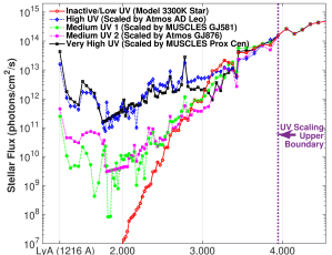
(a)

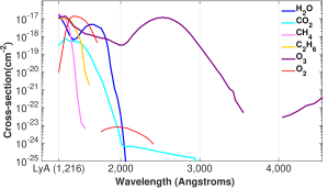
(b)

Figure 1: Top Panel: Earth-equivalent spectral energy distribution is shown for the inactive model star, with the four synthetically constructed < 3950 Å profiles overlaid. The spectra result from binning the original high resolution data over the Atmos wavelength grid for the UV cross-section data, after converting the flux density units from ergs/cm²/s/A^-1 to photons/cm²/s/A^-1 as expected by Atmos. The UV scaling boundary is marked at 3950 Å by the purple vertical line. Since we use real stellar UV data for the scaling, the difference amongst the profiles is not particularly dramatic after the binning. Earth-equivalent fluxes are obtained by taking the original stellar data and dividing by the solar constant. Bottom Panel: Available UV cross-section data used by Atmos shown for the species relevant to our 1-D model results.

We create each synthetic UV spectrum by stitching the extracted data to our UV-quiet model flux data, after binning our stellar data to a pre-defined coarser wavelength grid used by default in Atmos (see Figure 1 grid). The "stitching together" is done by scaling the stellar data (up to 3950 Å), such that the value at 3950 Å matches the model star value. In sum: shortward of 3950 Å, we use the scaled extracted data; longward of 3950 Å, we use the model star flux. Atmos’ spectral database stores unscaled stellar flux data as Earth-equivalent incident flux values (S_o) (red spectrum in Figure 1). This means that the overall incident flux at the top of the atmosphere is 1.21 times the fluxes shown in Figure 1.

The AD Leo (spectral type: M3.5V) and GJ876 (M4V) spectra have been used in several recent 1-D simulation studies of planetary atmospheres using our photochemical model (Segura et al., 2005, 2010; Domagal-Goldman et al., 2014; Harman et al., 2015; Arney et al., 2017). Their scaled versions correspond to "High UV" and "Medium UV 2", respectively, in Figure 1. We assign the highest activity level ("Very High UV") to the scaled MUSCLES Proxima Centauri (M6V) data. The remaining case ("Medium UV1") corresponds to scaled GJ581 (M3V) MUSCLES UV spectra.

2.3 Photochemistry in the Atmosphere via Atmos

VPL’s Atmos has been used in 1-D photochemical and climate modeling of early Mars, and the Archean and modern Earth atmospheres. Atmos simulations of rocky exoplanets have helped define the HZ (Kopparapu et al., 2013a, b, 2014).

The photochemical model in Atmos (Arney et al., 2016, 2017) solves a set of nonlinear, coupled ordinary differential equations for the mixing ratios of all species at all heights using the reverse Euler method. The method is first order in time and uses second-order centered finite differences in space. The system of equations is explicitly formulated as time-dependent equations that are solved implicitly by a time-marching algorithm. The model is run to steady state to obtain the final mixing ratio profiles. In each step, the model measures the relative change of the concentration of each species in each layer of the atmosphere. When all species in all layers change less their concentrations by than 15% in the time step, the size of the time step grows. When this size is greater than 10¹⁷ seconds (~3 billion years) the model is considered to have reached the steady state (i.e. convergence). This means that the steady state solutions have stable chemical profiles on timescales of billions of years, assuming constant boundary conditions. These boundary conditions can include biological gas fluxes, volcanic outgassing, atmospheric escape and parametrization for ocean chemistry.

We use the species and reaction list of the existing "Modern Earth" template in Atmos. Note that our use of this template does not imply that we are attempting to reproduce modern Earth’s atmosphere; this template is used for its representative mixture of gases for a N₂-H₂O dominated planet. The base model has 193 forward chemical reactions and 40 photolysis reactions for 40 chemical species made from H, C, O, N, and S, 23 of which participate in photolysis. While CO₂ is kept constant at 360 ppm in all five models, other species are allowed to vary. While a thick CO₂ atmosphere could radiatively cool the middle atmosphere, acting as a bottleneck for H₂O loss to space, the Earth-like CO₂ amount we assume here should have a relatively minor effect on stratospheric temperatures (Wordsworth & Pierrehumbert, 2013).

We modify the boundary conditions to simulate an abiotic planet after Harman et al. (2015). In all five runs, we fix the surface flux of CH₄ to a 1-Earth mass planet abiotic production rate of 1x10⁸ molecules/cm²/s after Guzmán-Marmolejo et al. (2013). To determine the lower boundary conditions for the other varying species (Table 2 cont.), we assume the surface environment (atmosphere and ocean) obeys redox balance (i.e. free electrons are conserved), using the methodology by Harman et al. (2015). While the atmospheric model ensures redox balance in the atmosphere, we must tune the boundary conditions to prevent a redox imbalance in the oceans or on the planet’s surface. We do this in our model by changing the H₂ flux into the atmosphere so that there is no net deposition of oxidizing or reducing power into the oceans or onto the surface. Thus, we tune the H₂ flux across the five UV scenarios until atmosphere and ocean redox balance independently for each case. This ensures that the atmospheric concentrations we report here are sustainable over geological timescales with only geological (and not biological) fluxes.

H₂O is the only non-background species with mixing ratios provided by the GCM. So, instead of defining surface conditions, we fix the H₂O abundance profile below the tropopause to the mixing ratios of those levels from the GCM. We assume that the atmosphere is hydrostatic, and there is no atmospheric escape occurring. Photochemical reaction timescales are much shorter (seconds to hundreds of years) than the timescales of atmospheric escape (billions of years). Thus, it is reasonable to exclude the effects of H escape on the chemistry; escape should primarily impact the long term evolution of the atmosphere and not its steady state composition.

Table 2: Some key photochemical model species with boundary conditions

Species	Lower bound type	Lower bound value
O	$\nu$dep	1.
O2	$\nu$dep	1.5$\times$10-4
H2O	see table comment	from GCM result
H	$\nu$dep	1.
OH	$\nu$dep	1.
HO2	$\nu$dep	1.
H2O2	$\nu$dep	2.$\times$ 10-1
H2	$\nu$dep, flux, disth	2.4$\times$10-4, 4.$\times$105- 2.$\times$1010, 1.
CO	$\nu$dep	1.$\times$10-8
CO2	fCO2	3.6$\times$10-4
HCO	$\nu$dep	1.
H2CO	$\nu$dep	2.$\times$10-1
CH4	flux	1.$\times$108
CH3	$\nu$dep	1.
C2H6	$\nu$dep	0.
NO	$\nu$dep	3.$\times$10-4
NO2	$\nu$dep	3.$\times$10-3
HNO	$\nu$dep	1.
O3	$\nu$dep	7.$\times$10-2
HNO3	$\nu$dep	2.$\times$10-1
N	$\nu$dep	0.
NO3	$\nu$dep	0.
N2O	$\nu$dep	0.
HO2NO2	$\nu$dep	2.$\times$10-1
N2O5	$\nu$dep	0.
N2	fixedN2	0.9956

The vertical grid is distributed evenly over 200 levels and extends to a TOA altitude of 91 km. The lower boundary pressure is set at 1 bar and the upper at 8.1x10^-7 bar. Both chemistry and vertical transport are considered for the 40 long-lived species. Transport is neglected for the 9 additional short-lived species such as O(¹D). For the long-lived species, vertical transport is approximated with a profile of eddy diffusion coefficients. Typically, these coefficients are patterned after eddy diffusivities that best reproduce modern-day Earth (Kasting, 1979, 1990). However, the vertical mixing has been shown to be stronger for Earth-like planets with slow rotation rates, owing to the aforementioned strong substellar convection. Thus for our runs, we adopt a constant eddy profile by iteratively determining a single eddy coefficient value (K_zz = 8.95 x 10⁶ cm²s^-1) that allows us to maintain the original GCM H₂O mixing ratio at 1 mbar, while letting the atmosphere column above vary. Above 1 mbar, we expect photochemistry to dominate over the vertical mixing.

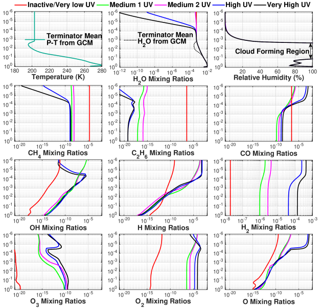
Figure 2: Steady state mixing ratio profiles computed by the photochemical model are shown for all varying non-trace species of interest. 1-D model input for the terminator mean H₂O (dotted-black in the H₂O panel) and $P$-$T$ (dark cyan) profiles from the GCM simulation are shown next to each other for interpretation. With the exception of the H₂ and H₂O panels, all other species are shown on the same wide mixing ratio scale for easy visual comparison. Relativity humidity profiles from the 1-D model for the resulting atmospheres are also shown, with the cloud condensation pressure range indicated within the panel.

2.4 Radiative Transfer Spectra via Exo-Transmit

Exo-Transmit is an open source software package to calculate exoplanet transmission spectra. Here we use Exo-Transmit to generate spectra from the computed steady state mixing ratios of all species for which spectral contribution has been established in IR, including trace species for which opacity data is available in the package.

Exo-Transmit is designed to generate spectra of planets with a wide range of atmospheric composition, temperature, surface gravity, size and host star. There is also an option to include an optically thick gray "cloud" deck at a user-specified pressure above the surface. As this cloud deck is not modeled from actual particles, wavelength-dependent cloud properties are not involved. This simply serves as a reasonable method for incorporating the effects of optical thick cloud layers in simulated transmission calculations. When this feature is employed, the transit base is raised to the user-specified cloud-top pressure, meaning data pertaining to the atmosphere column below this pressure level is not read. Our purpose is to quantify spectral differences stemming from varying the UV alone; we keep the transit radius at the model base of 1 bar in our simulations, thus calculating the maximum signal that we would obtain for these atmospheres. We do, however, utilize the cloud truncation feature to compare our spectra to the spectrum shown in Kopparapu et al. (2017), which did include clouds (see Section 4). Exo-Transmit is available publicly on Github with open-source licensing at https://github.com/elizakempton/Exo_Transmit.

Exo-Transmit comes with pre-defined P-T and mixing ratio profiles binned to the resolution of its opacity data, where the pressure grid spans 10^-9 - 10³ bar in logarithmic steps of one dex (i.e. $P$ = 10^$n$, where $n$ is an integer). For our study, we replace these input files with our own ones containing the newly computed mixing ratios and the mean terminator P-T profile. Our P-T profile is much more finely sampled than Exo-Transmit’s opacity/chemistry grid. During each run of Exo-Transmit, the opacity is first interpolated onto each point of our P-T grid, then the radiative transfer calculation is run to compute the net spectrum.

3 Results

3.1 Atmospheric Constituent Mixing Ratio Profiles

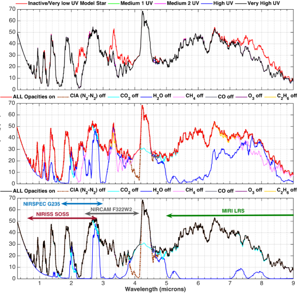
Figure 3: Top panel: Full spectra from Exo-Transmit shown for all five UV scenarios. Spectra assume there are no clouds. The four synthetic UV active cases completely overlap, with a slight mismatch at 4.3 µm due to CO differences. Middle panel: Full spectra from the inactive model star case shown (red, per Figure 2’s convention), along with individual contributions removed. Bottom panel: Full spectra for the Very High UV case (black, also same convention) shown this time, along with the same individual species removed. The JWST instrument bandpasses where prominent H₂O features occur have also been indicated here.

Although the two Medium UV spectra have much higher UV levels than the inactive model spectra at wavelengths < 3950Å, with ~10 orders of magnitude difference at 1216 Å (Figure 1), we find neither of them to be high enough to cause appreciable H₂O loss (see top of H₂O panel in Figure 2).

In the inactive model star case–where no photolytic loss is noted for any of the species shown–we see high constant values for the CH₄ and C₂H₆ mixing ratios being maintained over the entire atmosphere. The CH₄ source in this abiotic atmosphere is dominated by the lower boundary constant upward flux (flux = 1$\times$10⁸ molecules/cm²/s in Table 2). So we can expect total CH₄ production to be similar across all five cases. For the four UV-active cases, higher UV would translate to higher total loss of CH₄ due to photolysis. CH₃ is a highly reactive product of CH₄ photolysis and combines with itself to produce C₂H₆, which also photodisassociates and cycles back into CH₄; the three hydrocarbons cycle amongst themselves. The dominant exit pathway from this cycle - reaction of CH₃ with oxidants - is limited by the rate of CH₄ + OH —> CH₃ + H₂O. Thus, CH₄ chemistry is dominated by the abundance of OH in the atmosphere, as evidenced by a negative correlation between the OH and CH₄ profiles. The higher the OH abundance, the higher the CH₄ loss via combination with OH. This is also demonstrated by our examination of the sinks for CH₄; for UV-active stars, destruction of CH₄ is dominated by reaction with OH, and this rate even outpaces our abiotic surface CH₄ flux. The net impact of this chemistry is much lower abundances for CH₄ and C₂H₆ for the UV-active stars compared to the inactive model star.

OH is primarily produced in the atmosphere via H₂O photolysis. Our Medium UV stars show similar Ly-$\alpha$ strengths, so the resultant H₂O photolysis rates are also similar. For the High UV and Very High UV stars–both with synthetic UV ~2 orders of magnitude higher than the Medium UV stars–we see significant H₂O loss: the High UV star depletes TOA H₂O by ~6 orders of magnitude; while the Very High UV star depletes the TOA H₂O by ~3 further orders of magnitude. Ly-$\alpha$ strength is slightly higher in the Very High UV spectra.

Like most species in our model, atomic O, O₂, and O₃, have only been defined by lower boundary deposition efficiency values. Without a surface source of O₂ and O₃, atmospheric chemistry is their only source. Thus, their concentrations are minor for the inactive star (red profiles in Figure 2). As UV increases, we see higher abundances in all three species, especially O₂ and O₃, although their presence remains below detectable levels. At high altitudes, both O and O₂ generally increase in concentration, consistent with having a photolytic source. O₂ maintains high abundance throughout the column for the highest UV cases as the UV flux is quite high in both spectra between 1300-1500 Å, where the O₂ UV cross-section curve peaks. Although far UV activity is important for O₃ production, O₃ remains minor throughout the atmosphere even for the highest UV case. O₃ is produced in the model by the three-body reaction O + O₂ —> O₃ and this is the only mechanism that produces it in this atmosphere. Otherwise, O₃ is being destroyed via photolysis reactions O₃ + h$\nu$ —> O₂ + O(¹D) and O₃ + h$\nu$ —> O₂ + O, along with 10 other chemical reactions. When O₃ is destroyed via these pathways, O₂ is always produced.

3.2 Transmission Spectra

For all cases considered, with no cloud cover, we obtain large H₂O features–around 50 ppm in strength–between 2.5-3.8 µm and 4.5-9 µm (Figure 3). The locations where these H₂O features peak are consistent with Figure 11 of Kopparapu et al. (2017) (Figure 4). The 2.5-3.8 µm feature peaks within the JWST NIRCam grism with the F322W2 filter, as well as the NIRSPEC G235M/H and NIRISS SOSS (Single Object Slitless Spectroscopy) bandpasses. The 4.5-9 µm feature is well within the JWST MIRI LRS (Low Resolution Spectroscopy) bandpass. For the model star case, we also see additional absorption at 2.2 µm, 3.3 µm and 7.4-8.4 µm (i.e. the red profile minus the black profile in the top panel of Figure 3), caused by the high CH₄ (>10^-5) predicted by the model for our choice of CH₄ lower boundary condition.

CO₂ produces the tallest feature in our spectra (Figure 3). This narrow feature at 4.3 µm (~0.4 µm wide when measured from the brown dotted spectrum) is ~20 ppm larger than the H₂O features, and 40 ppm larger than the N₂-N₂ collision induced absorption (CIA) feature it overlaps. This region falls within the bandpasses of the NIRCAM F444W filter (3.8-4.8 µm) as well as the NIRSPEC G333/H grating (2.9-5 µm).

The N₂-N₂ CIA feature spans the 3.8 to 5 µm wavelength range (cyan colored bumps in Figure 3). This opacity source stems from the deep atmosphere (right panel of Figure 4) and is strong due to the high N₂ (Schwieterman et al., 2015) content of the atmosphere. This implies we may be able to quantify atmospheric N₂ from this feature’s strength in a cloudless atmosphere. As evident from the two spectra shown with CIA removed (brown dotted plots in Figure 3), the base of the 4.3 µm CO₂ feature is broadened by the CIA feature but the height is unaffected; this feature is the only other absorption feature occurring between 4 µm and the CO₂ feature.

While O₂ is significantly enhanced with increasing UV, it is spectrally insignificant. The few features from O₂ molecular and collision induced opacities occur < 1.0 µm and are completely masked by the Rayleigh tail. Atomic O is enhanced at high altitudes, but there is no atomic opacity for O. O₃ can be spectrally important in IR as it produces molecular and collision induced features at wavelengths longer than 1.1 µm. O₃ acts as a UV shield for atmospheres where it is present (e.g. Earth) and thus has important consequences for habitability (Rugheimer et al., 2015b, a). O₃ appears to have no impact on any of the spectra we have presented here.

Most importantly, Figure 3 (top panel) shows that spectra from the UV active runs overlap almost completely. However, in the inactive model star’s case, additional absorptions longward of the peak H₂O features stem primarily from the high CH₄ and some from C₂H₆. C₂H₆ contribution is most noteworthy at 3.3 µm, where it also overlaps with major contribution from CH₄ and H₂O, and then from 6.5-7.4 µm, where most of the contribution is still from H₂O. These demonstrate the impact of M dwarf UV activity on the planet’s transit observations. We find that for any realistic levels of UV radiation from an M dwarf host star, the atmospheric response to the amount of radiation is undetectable.

From our 1-D modeling results, we infer that H₂O photodissociation from high UV instellation does not impact transmission spectra, and thus should not affect our ability to detect H₂O absorption features from a habitable synchronously rotating Earth-like planet around a nearby M dwarf. This is expected as transmission features should primarily originate from lower regions of the atmosphere $\geq$ 1 mbar (left panel of Figure 4). In the upper atmosphere above the substellar clouds, there is no reason for the planet-wide vertical mixing driven by strong convection to continue dominating. Thus photochemistry can dominate here, meaning we cannot expect H₂O to stay enriched. Accordingly, we only note visible impact from photochemistry above the stratosphere (and cloud decks) for all species involved in photolysis in the modeled atmospheres (Figure 2).

4 Discussion

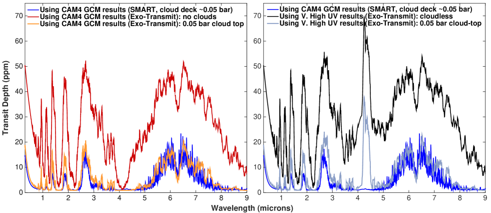
Figure 4: Left panel: Exo-Transmit spectra computed using terminator mean mixing ratios from the pure N₂-H₂O atmosphere (GCM results) shown alongside the Kopparapu et al. (2017) SMART version of it (blue). As the water clouds occur ~0.05 bar in the SMART computations, we also include the spectrum that results from placing an opaque cloud at 0.05 bar within Exo-Transmit. Exo-Transmit spectra shown here have CIA turned off for direct comparison; the SMART spectrum does not include CIA. The CIA opacity has a minimal effect on these spectra so their inclusion or non-inclusion is not a dominant factor in the modeling outcomes. Right panel: Very High UV Exo-Transmit spectra shown for cloudless (same black spectrum from Figure 3) and 0.05 bar cloud top (gray) cases, in comparison to the SMART spectrum of the GCM results. Note that the difference in the 4-5 um range between the GCM + SMART simulation (in blue) and the GCM + PHOTOCHEM + Exo-transmit simulations (gray/black spectrum) is due to the inclusion of CO₂ in the photochemical models, but not in the GCM, which assumed a pure N₂-H₂O atmosphere.

Figure 2 shows that water vapor concentration is highest between 0.1 and 1 bar, close to the surface as expected. The cold trap minimum is also found between two other Exo-Transmit pressure grid points. To ensure accuracy of our interpolations onto this coarse pressure grid, we have experimented with shifting the cold trap altitude. Of-course, the transit depths shown in Figure 3 should still not be taken at face value; moist atmospheres have water clouds that are not accounted for here. Since Exo-Transmit does not presently have the capability to include specific cloud properties, we do not include the liquid and ice data from the GCM run outputs as part of our spectral analysis. We see the impact of such water clouds in the transmission spectra provided in Kopparapu et al. (2017), computed by VPL’s Spectral Mapping Atmospheric Radiative Transfer (SMART) tool for the planet-star configuration we have studied here. Data from the GCM simulation results were used directly in SMART to calculate the spectrum for the synchronously rotating planet.

We are able to compare our spectra with the SMART spectrum by raising the base altitude and thus sampling a lower pressure range (i.e. a shallower column) of the atmosphere in Exo-Transmit. For comparison, we compute spectrum for the original pure N₂-H₂O GCM atmosphere, with no photochemical alteration. We do this for a few cases with Exo-Transmit: a default case with the original 1 bar base, and some additional computations to simulate the effects of clouds by raising the spectral model base to successively lower pressures. In the left panel of Figure 4, we show the spectrum of the default case with no clouds, and the spectrum for a cloud-top pressure of 0.05 bar–the location of the water clouds in the SMART-computed version of the GCM results. For comparison, we overplot the spectrum from SMART. We see that by artificially truncating our spectra at this cloud-top pressure, we are able to capture most of the impacts of the clouds on the spectrum.

We validate the consistency of our Exo-Transmit calculations with the SMART spectrum by noting a reasonable overlap between the two cloudy spectra (in both panels). We see that the spectra diverge in the near-IR, for wavelengths shorward of 4 µm. The transit depths are consistently larger in the cloudy spectrum computed by Exo-Transmit for wavelengths shorter than 4 µm; Exo-Transmit computes a larger apparent size for these planets than SMART in the near-IR. Differences in the treatment of clouds (properties such as particle size, optical constants, etc.) between the two spectral models would be responsible for this kind of discrepancy. As we mentioned earlier in Section 2.4, Exo-Transmit treats its clouds as a fully gray optically thick deck, so cloud properties do not vary with wavelength. However, SMART has wavelength-dependent water cloud properties incorporated in the spectral modeling scheme. We believe the trend we are seeing in Figure 4 is a result of this.

Figure 4 (right panel) also shows that the CO₂ 4.3 µm feature remains prominent in the cloudy spectrum of the photochemical model results. The atmospheric column above 0.05 bar is still being transmitted and contributes to the spectrum. At 0.05 bar, the H₂O mixing ratio is ~2$\times$10^-3. Transit spectroscopy typically sample the planet at ~1 mbar atmospheric pressure, which is also the GCM TOA. The GCM TOA H₂O mixing ratio is ~5.55$\times$10^-4 (Figure 2, also see Table 1 of Kopparapu et al. (2017)). Since our CO₂ abundance is slightly less than that and also less than ~1/5th of the 0.05 bar H₂O abundance, the much higher CO₂ transit depth signal is noteworthy for future observing efforts.

Greene et al. (2016) has suggested systematic noise floors of ~20 ppm for NIRISS/NIRSpec and ~30 ppm for the NIRCam grism, which is not only well below the CO₂ 4.3 µm signal strength for the cloudless case, but is also comparable to the difference between this feature and the largest H₂O features. These observational advantages still hold for the 0.05 bar cloud top spectra. So in a similarly cloudy atmosphere but with modern Earth-like amounts of CO₂, the CO₂ may be more readily detected. Of-course, the true performance of the instruments will only be known once JWST actually flies.

One issue that can impact our quantitative predictions of O₂ and O₃ is how Atmos treats CO₂. Atmos presently accepts CO₂ as a user-specified constant mixing ratio for terrestrial planets, though it allows for CO₂ production and destruction reactions, including photolysis (CO₂ + h$\nu$ —> CO + O and CO₂ + h$\nu$ —> CO + O(¹D)). So a caveat here is that the model produces excess CO₂ in order to maintain the constant 360 ppm CO₂ abundance. This overestimates both the upper atmosphere CO₂ abundance and the total O budget. This could be important for the computed O₂ and O₃ mixing ratios. However, since we note photochemical effects only above the column of the atmosphere sampled by transits, a major impact on transit observations is unlikely and this impact is mostly just quantitative. For now, we save discussion of O₃ absorption features for a subsequent manuscript focused more on O chemistry.

H₂ and CH₄ are the only non-negligible species in our model defined by lower boundary flux values (see Table 2) that also dominate their source functions. The higher the stellar UV flux, the higher the H₂ flux value needs to be to achieve global redox balance for a given CH₄ flux. H and OH trends across the models are thus affected by the varying H₂ source. We keep the CH₄ flux fixed in this study as small changes to this flux do not have an impact on the concentrations of gases for which we note detectable spectral features in Figures 3 and 4. Further investigation of the effects of the choice of CH₄ flux on the abundances and detectability of relatively trace species will be explored in a future paper.

5 Conclusions

We have taken a synchronously orbiting aquaplanet-star pair result from Kopparapu et al. (2017) within the stable moist habitable regime, and have conducted a case study on its future detectability via JWST. We have investigated the impact of stellar activity on the detection of terrestrial planets with water-rich stratospheres, as photolysis from high UV activity would continuously destroy the water lofted into the high atmosphere. We have run five photochemical models, each with different wavelength-dependent UV activity, ranging from the inactive model (BT-Settl) star data used in Kopparapu et al. (2017) to Proxima Centauri-like levels. We have used stellar fluxes from the VPL spectral database in Atmos and the MUSCLES Treasury Survey to vary the UV levels.

We find that as long as the atmosphere is well-mixed up to 1 mbar, H₂O strengths observed in transit spectra should remain unaffected by UV activity. However, for the inactive model star, transit depths are larger due to contributions from the high CH₄ in the atmosphere for our specified CH₄ surface flux, which assumes Earth-like abiotic sources of CH₄. Detectable CH₄ is absent in the UV active cases.

CO₂ produces a narrow but large detectable feature at 4.3 µm. For our assumed atmospheric CO₂ level of 360 ppm, this feature is about 20 ppm larger than the tallest H₂O features. At the wavelengths where CO₂ does overlap H₂O features, the maximum contribution is also 20 ppm over a very narrow (<1 µm broad) region at 2 µm (i.e. before the prominent H₂O features appear) for a cloudless case. We also see broadening of the base of the 4.3 µm CO₂ feature due to opacity from N₂-N₂ collisional pairs. However, upon comparing the two "Very High UV" spectra in the right panel of Figure 4, we see that the N₂-N₂ CIA feature is a high pressure feature originating from well below cloud decks. Thus, the CIA feature should not contribute to the observed signal from CO₂ in practice.

While UV activity may not impact transit depths at the ppm level, water clouds do. Upon comparing the cloud-containing SMART spectrum from Kopparapu et al. (2017) for the synchronously rotating planet modeled by the GCM, with a cloud-free version of it from Exo-Transmit, we find that the 0.05 bar cloud weakens the strongest H₂O feature at 6 µm from 50 ppm—comparable to the postulated MIRI systematic noise floor—to only 15 ppm. This means should the terminator cloud deck occur lower in the atmosphere, at pressures > 0.05 bar, we should require less observing time to make a positive detection. Overall, we see few detectable impacts of photochemistry on the spectra of these worlds.

References

- Allard et al. (2007) Allard, F., Allard, N. F., Homeier, D., et al. 2007, A&A, 474, L21, ADS, 0709.1192
- Allard et al. (2003) Allard, F., Guillot, T., Ludwig, H.-G., et al. 2003, in IAU Symposium, Vol. 211, Brown Dwarfs, ed. E. Mart´n, 325, ADS
- Allen et al. (1980) Allen, M., Yung, Y. L., & Pinto, J. P. 1980, ApJ, 242, L125, ADS
- Arney et al. (2016) Arney, G., Domagal-Goldman, S. D., Meadows, V. S., et al. 2016, Astrobiology, 16, 873, ADS, 1610.04515
- Arney et al. (2017) Arney, G. N., Meadows, V. S., Domagal-Goldman, S. D., et al. 2017, ApJ, 836, 49, ADS, 1702.02994
- Benneke & Seager (2013) Benneke, B., & Seager, S. 2013, ApJ, 778, 153, ADS, 1306.6325
- Bétrémieux & Kaltenegger (2015) Bétrémieux, Y., & Kaltenegger, L. 2015, MNRAS, 451, 1268, ADS, 1507.02107
- Bin et al. (2018) Bin, J., Tian, F., & Liu, L. 2018, EPSL, 492, 121, ADS
- Chapman (1930a) Chapman, S. 1930a, The London, Edinburgh, and Dublin Phil Mag and Journal of Sci, 10, 345, https://doi.org/10.1080/14786443009461583
- Chapman (1930b) Chapman, S. 1930b, The London, Edinburgh, and Dublin Phil Magazine and Journal of Sci, 10, 369, https://doi.org/10.1080/14786443009461588
- Chapman (1942) Chapman, S. 1942, Reports on Progress in Physics, 9, 92
- Crisp (1997) Crisp, D. 1997, Geophys. Res. Lett., 24, 571, ADS
- Domagal-Goldman et al. (2014) Domagal-Goldman, S. D., Segura, A., Claire, M. W., et al. 2014, ApJ, 792, 90, ADS, 1407.2622
- Fujii et al. (2018) Fujii, Y., Angerhausen, D., Deitrick, R., et al. 2018, Astrobiology, 18, 739, ADS, 1705.07098
- Fujii et al. (2017) Fujii, Y., Del Genio, A. D., & Amundsen, D. S. 2017, ApJ, 848, 100, ADS, 1704.05878
- Greene et al. (2016) Greene, T. P., Line, M. R., Montero, C., et al. 2016, ApJ, 817, 17, ADS, 1511.05528
- Guzmán-Marmolejo et al. (2013) Guzmán-Marmolejo, A., Segura, A., & Escobar-Briones, E. 2013, Astrobiology, 13, 550, ADS
- Haqq-Misra et al. (2018) Haqq-Misra, J., Wolf, E. T., Joshi, M., et al. 2018, ApJ, 852, 67, ADS, 1710.00435
- Harman et al. (2015) Harman, C. E., Schwieterman, E. W., Schottelkotte, J. C., et al. 2015, ApJ, 812, 137, ADS, 1509.07863
- Heng & Demory (2013) Heng, K., & Demory, B.-O. 2013, ApJ, 777, 100, ADS, 1309.5956
- Hu et al. (2012) Hu, R., Seager, S., & Bains, W. 2012, ApJ, 761, 166, ADS, 1210.6885
- Kasting (1979) Kasting, J. F. 1979, PhD thesis, Michigan Univ., Ann Arbor
- Kasting (1990) Kasting, J. F. 1990, Origins of life and evolution of the biosphere, 20, 199
- Kasting et al. (1993) Kasting, J. F., Whitmire, D. P., & Reynolds, R. T. 1993, Icarus, 101, 108, ADS
- Kempton et al. (2017) Kempton, E. M.-R., Lupu, R., Owusu-Asare, A., et al. 2017, PASP, 129, 044402, ADS, 1611.03871
- Knutson et al. (2014) Knutson, H. A., Benneke, B., Deming, D., et al. 2014, Nature, 505, 66, ADS, 1401.3350
- Kopparapu et al. (2012) Kopparapu, R. k., Kasting, J. F., & Zahnle, K. J. 2012, ApJ, 745, 77, ADS, 1110.2793
- Kopparapu et al. (2013a) Kopparapu, R. K., Ramirez, R., Kasting, J. F., et al. 2013a, ApJ, 765, 131, ADS, 1301.6674
- Kopparapu et al. (2014) Kopparapu, R. K., Ramirez, R. M., SchottelKotte, J., et al. 2014, ApJ, 787, L29, ADS, 1404.5292
- Kopparapu et al. (2017) Kopparapu, R. K., Wolf, E. T., Arney, G., et al. 2017, ApJ, 845, 5, ADS, 1705.10362
- Kopparapu et al. (2016) Kopparapu, R. K., Wolf, E. T., Haqq-Misra, J., et al. 2016, ApJ, 819, 84, ADS, 1602.05176
- Kopparapu et al. (2013b) Kopparapu, R. K., et al. 2013b, ApJ, 767, L8, ADS, 1303.2649
- Krasnopolsky & Pollack (1994) Krasnopolsky, V. A., & Pollack, J. B. 1994, Icarus, 109, 58, ADS
- Kreidberg et al. (2014) Kreidberg, L., Bean, J. L., Désert, J.-M., et al. 2014, Nature, 505, 69, ADS, 1401.0022
- Kreidberg et al. (2018) Kreidberg, L., Line, M. R., Thorngren, D., et al. 2018, ApJ, 858, L6, ADS, 1709.08635
- Leconte et al. (2015) Leconte, J., Wu, H., Menou, K., et al. 2015, Science, 347, 632, ADS, 1502.01952
- Liang et al. (2003) Liang, M.-C., Parkinson, C. D., Lee, A. Y.-T., et al. 2003, ApJ, 596, L247, ADS, astro-ph/0307037
- Liang et al. (2004) Liang, M.-C., Seager, S., Parkinson, C. D., et al. 2004, ApJ, 605, L61, ADS, astro-ph/0402601
- Line & Yung (2013) Line, M. R., & Yung, Y. L. 2013, ApJ, 779, 3, ADS, 1309.6679
- Mbarek & Kempton (2016) Mbarek, R., & Kempton, E. M.-R. 2016, ApJ, 827, 121, ADS, 1602.02759
- Meadows & Crisp (1996) Meadows, V. S., & Crisp, D. 1996, J. Geophys. Res., 101, 4595, ADS
- Merlis & Schneider (2010) Merlis, T. M., & Schneider, T. 2010, Journal of Advances in Modeling Earth Systems, 2, 13, ADS, 1001.5117
- Miller-Ricci Kempton et al. (2012) Miller-Ricci Kempton, E., Zahnle, K., & Fortney, J. J. 2012, ApJ, 745, 3, ADS, 1104.5477
- Misra et al. (2014) Misra, A., Meadows, V., & Crisp, D. 2014, ApJ, 792, 61, ADS, 1407.3265
- Morley et al. (2017) Morley, C. V., Knutson, H., Line, M., Fortney, J. J., Thorngren, D., Marley, M. S., Teal, D., & Lupu, R. 2017, AJ, 153, 86, ADS, 1610.07632
- Moses et al. (2013) Moses, J. I., Line, M. R., Visscher, C., et al. 2013, ApJ, 777, 34, ADS, 1306.5178
- Moses et al. (2011) Moses, J. I., Visscher, C., Fortney, J. J., et al. 2011, ApJ, 737, 15, ADS, 1102.0063
- Neale et al. (2010) Neale, R. B., Chen, C. C., Gettelman, A., et al. 2010, Description of the NCAR Community Atmosphere Model (CAM 5.0), NCAR/TN-486+STR NCAR Technical Note
- Noda et al. (2017) Noda, S. et al. 2017, Icarus, 282, 1, ADS
- Rugheimer et al. (2015a) Rugheimer, S., Kaltenegger, L., Segura, A., et al. 2015a, ApJ, 809, 57, ADS, 1506.07202
- Rugheimer et al. (2015b) Rugheimer, S., Segura, A., Kaltenegger, L., et al. 2015b, ApJ, 806, 137, ADS, 1506.07200
- Schwieterman et al. (2015) Schwieterman, E. W., Robinson, T. D., Meadows, V. S., et al. 2015, ApJ, 810, 57, ADS, 1507.07945
- Segura et al. (2005) Segura, A., Kasting, J. F., Meadows, V. S., et al. 2005, Astrobiology, 5, 706, ADS, astro-ph/0510224
- Segura et al. (2010) Segura, A., Walkowicz, L. M., Meadows, V., et al. 2010, Astrobiology, 10, 751, ADS, 1006.0022
- Shields et al. (2013) Shields, A. L., Meadows, V. S., Bitz, C. M., et al. 2013, Astrobiology, 13, 715, ADS, 1305.6926
- Visscher & Moses (2011) Visscher, C., & Moses, J. I. 2011, ApJ, 738, 72, ADS, 1106.3525
- Wakeford et al. (2017) Wakeford, H. R., Visscher, C., Lewis, N. K., et al. 2017, MNRAS, 464, 4247, ADS, 1610.03325
- Wakeford et al. (2015) Wakeford, H. R., et al. 2015, A&A, 573, A122, ADS, 1409.7594
- Wang et al. (2016) Wang, Y., Liu, Y., Tian, F., Yang, J., et al. 2016, ApJ, 823, L20, ADS
- Wang et al. (2014) Wang, Y., Tian, F., & Hu, Y. 2014, ApJ, 791, L12, ADS
- Way et al. (2016) Way, M. J., Del Genio, A. D., Kiang, N. Y., et al. 2016, Geophys. Res. Lett., 43, 8376, ADS, 1608.00706
- Wolf (2017) Wolf, E. T. 2017, ApJ, 839, L1, ADS, 1703.05815
- Wolf & Toon (2013) Wolf, E. T., & Toon, O. B. 2013, Astrobiology, 13, 656, ADS
- Wolf & Toon (2014) Wolf, E. T., & Toon, O. B. 2014, Geophys. Res. Lett., 41, 167, ADS
- Wolf & Toon (2015) Wolf, E. T., & Toon, O. B. 2015, JGRD, 120, 5775, ADS
- Wordsworth & Pierrehumbert (2013) Wordsworth, R. D., & Pierrehumbert, R. T. 2013, ApJ, 778, 154, ADS, 1306.3266
- Yang et al. (2014a) Yang, J., Boué, G., Fabrycky, D. C., et al. 2014a, ApJ, 787, L2, ADS, 1404.4992
- Yang et al. (2013) Yang, J., Cowan, N. B., & Abbot, D. S. 2013, ApJ, 771, L45, ADS, 1307.0515
- Yang et al. (2016) Yang, J., Leconte, J., Wolf, E. T., et al. 2016, ApJ, 826, 222, ADS
- Yang et al. (2014b) Yang, J., Liu, Y., Hu, Y., et al. 2014b, ApJ, 796, L22, ADS, 1411.0540
- Youngblood et al. (2016) Youngblood, A., France, K., Loyd, R. O. P., et al. 2016, ApJ, 824, 101, ADS, 1604.01032
- Yung et al. (1984) Yung, Y. L., Allen, M., & Pinto, J. P. 1984, ApJS, 55, 465, ADS
- Yung & Demore (1982) Yung, Y. L., & Demore, W. B. 1982, Icarus, 51, 199, ADS
- Zahnle et al. (2009a) Zahnle, K., Marley, M. S., & Fortney, J. J. 2009a, ArXiv e-prints, ADS, 0911.0728
- Zahnle et al. (2009b) Zahnle, K., Marley, M. S., Freedman, R. S., et al. 2009b, ApJ, 701, L20, ADS, 0903.1663