Iteratively reweighted penalty alternating minimization methods with continuation for image deblurring

Abstract

In this paper, we consider a class of nonconvex problems with linear constraints appearing frequently in the area of image processing. We solve this problem by the penalty method and propose the iteratively reweighted alternating minimization algorithm. To speed up the algorithm, we also apply the continuation strategy to the penalty parameter. A convergence result is proved for the algorithm. Compared with the nonconvex ADMM, the proposed algorithm enjoys both theoretical and computational advantages like weaker convergence requirements and faster speed. Numerical results demonstrate the efficiency of the proposed algorithm.

Index Terms—  Nonconvex alternating minimization, Penalty method, Continuation, Total Variation, Image deblurring

1 Introduction

Linearly constrained problems are widely discussed through various disciplines such as image sciences, signal processing and machines learning, to name a few. The classical algorithm for the linearly constrained problems is the Alternating Direction Method of Multiplier (ADMM); and the previous literature has paid their attention to the convex case [1, 2, 3, 4]. In recent years, nonconvex ADMM has been developed for the nonconvex problems [5, 6, 7, 8].

1.1 Motivations

Although ADMM can be applied to the nonconvex Total Variation (TV) deblurring problem, several drawbacks still exist. We point out three of them as follows.

1. The convergence guarantees of nonconvex ADMMs require a very large Lagrange dual multiplier. Worse still, the large multiplier makes the nonconvex ADMM run slowly.

2. When applying nonconvex ADMMs to the nonconvex TV deblurring model, by direct checks, the convergence requires TV operator to be full row-rank; however, the TV operator cannot promise such an assumption. This point has been proposed in [9].

3. The previous analyses show that the sequence converges to a critical point of an auxiliary function under several assumptions. But the relationship between the auxiliary function and the original one is unclear in the nonconvex settings.

Considering these drawbacks, from both computational and theoretical perspectives, it is necessary to consider novel and efficient solvers. The main reason why nonconvex ADMMs have these drawbacks is due to the dual variable; in the convergence proof of the nonconvex case, the dual variables are just simply processed by Cauchy inequalities; the deductions in the proofs are then somehow loose. Therefore, we consider employing the penalty method to avoid using the dual information.

1.2 Contributions and organization

In this paper, we consider using the penalty method for a class of nonconvex linearized constrained minimizations. Different from the nonconvex ADMM, determining the penalty multiplier in the proposed algorithm is very lowly-costly. Although the penalty multiplier is also large, we can use a continuation method, i.e., increasing the penalty multiplier in the iteration. The alternating minimization methods [10, 11] are fit for solving this penalty problem. Directly applying the alternating minimization for the penalty problem encounters an issue: the subproblem may have no closed form. To overcome this problem, combining the structure of the problem, we use the linearized techniques for the regularized part in the algorithm. In this way, all the subproblems are convex and can be minimized numerically globally even without enjoying a closed form solution. We proved the square-summability of the successive differences of the generated points. We apply our algorithm to the nonconvex image delurring problem and compare it with the nonconvex ADMM. The numerics show the efficiency and speed of the proposed algorithm.

In Section 2, we present our problem and algorithm, and the convergence results of the algorithm. Section 3 contains the applications and numerics. And then Section 4 concludes the paper.

2 Problem formulation and algorithm

In this paper, we consider a broad class of nonconvex and nonsmooth problems with the following form:

$$\min_{x,y}\{\Psi(x,y):=f(x)+\sum_{i=1}^{N}h(g(y_{i})),~{}\textrm{s.t.}~{}Ax+By=c\}.$$ (1)

where $x\in\mathbb{R}^{M},y\in\mathbb{R}^{N}$, and functions $f$, $g$ and $h$ satisfy the following assumptions:

• A.1 $f:\mathbb{R}^{M}\rightarrow\mathbb{R}$ is a closed proper convex function and $\inf_{x\in\mathbb{R}^{M}}f(x)>-\infty$.

• A.2 $g:\mathbb{R}\rightarrow\mathbb{R}$ is a convex function, and the proximal map of $g$ is easy to calculated.

• A.3 $h:\textrm{Im}(g)\rightarrow\mathbb{R}$ is a concave function and $\inf_{t\in\textrm{Im}(g)}h(t)>-\infty$.

A very classical problem which can be formulated as (1) is Total Variation $q$ (TV-$q$) deblurring [12]

$$\min_{u}\{\frac{1}{2}\|H(u)-B\|_{F}^{2}+\lambda\|T(u)\|_{q}^{q}\},$$ (2)

where $H$ is the blurring operator, $T$ is the well-known total variation operator and $q\in(0,1)$. By defining $v:=T(u)$, the problem then turns to

$$\min_{u,v}\{\frac{1}{2}\|H(u)-B\|_{F}^{2}+\lambda\|v\|_{q}^{q}~{}~{}\textrm{s.t.}~{}~{}v=T(u)\}.$$ (3)

2.1 Algorithm

We consider the penalty function as

$$\min_{x,y}\{\Phi_{\gamma}(x,y):=f(x)+\sum_{i=1}^{N}h(g(y_{i}))+\frac{\gamma}{2}\|Ax+By-c\|_{2}^{2}\}.$$ (4)

The difference between problem (1) and (4) is determined by the parameter $\gamma$. They are identical if $\gamma=+\infty$. Assume that $(x^{*},y^{*})$ is the solution to problem (4), and $(x^{{\dagger}},y^{{\dagger}})$ is the solution to problem (1), and $(\hat{x},\hat{y})$ is any one satisfying $A\hat{x}+B\hat{y}=c$, we then have the following claims.

$$\Psi(x^{*},y^{*})\leq\Psi(x^{{\dagger}},y^{{\dagger}})$$ (5)

and

$$\|Ax^{*}+By^{*}-c\|_{2}^{2}\leq\frac{2}{\gamma}[\Psi(\hat{x},\hat{y})-\underline{f}-\underline{h_{g}}],$$ (6)

where $\inf_{x\in\mathbb{R}^{M}}f(x)\geq\underline{f}$ and $\inf_{t\in\textrm{Im}(g)}h(t)\geq\underline{h_{g}}$. These two claims can provide the errors between (1) and (4). We present brief proofs for claims (5) and (6). First, with the definition of $(x^{*},y^{*})$, we have

$$\Phi_{\gamma}(x^{*},y^{*})\leq\Phi_{\gamma}(x^{{\dagger}},y^{{\dagger}}).$$ (7)

Noting $Ax^{{\dagger}}+By^{{\dagger}}=c$, we then have

$$\Psi(x^{*},y^{*})+\frac{\gamma}{2}\|Ax^{*}+By^{*}-c\|_{2}^{2}\leq\Psi(x^{{\dagger}},y^{{\dagger}}).$$ (8)

Thus, we are led to

$$\Psi(x^{*},y^{*})\leq\Psi(x^{{\dagger}},y^{{\dagger}}).$$ (9)

Similarly, we derive

$$\Psi(x^{*},y^{*})+\frac{\gamma}{2}\|Ax^{*}+By^{*}-c\|_{2}^{2}\leq\Psi(\hat{x},\hat{y}).$$ (10)

With the fact $\Psi(x^{*},y^{*})\geq\inf_{x\in\mathbb{R}^{M}}f(x)+\inf_{t\in\textrm{Im}(g)}h(t)$, we then get (6).

We apply the claims to the TV deblurring problem (3), we can see $\inf_{u}\|H(u)-B\|_{2}^{2}\geq 0,\inf_{v}\|v\|_{q}^{q}\geq 0$; and we can choose $\hat{u}=\textbf{0}$ and $\hat{v}=\textbf{0}$. Then, it holds

$$\|Tu^{*}-v^{*}\|_{2}^{2}\leq\frac{2\|B\|^{2}_{2}}{\gamma},$$

where $(u^{*},v^{*})$ is the minimizer of the penalty problem. Thus, to achieve $\varepsilon$ error approximation, we just need to set $\gamma=\frac{2\|B\|^{2}_{2}}{\varepsilon}$.

The classical algorithm solving this problem is the Alternating Minimization (AM) method, i.e., minimizing one variable while fixing the other one. However, if directly applying AM to model (4), the subproblem may still be nonconvex; the minimizer is hard to obtain in most cases. Considering the structure of the problem, we use a linearized technique for the nonsmooth part $\sum_{i=1}^{N}h(g(y_{i}))$. This method was inspired by the reweighted algorithms [13, 14, 15, 16]. To derive the sufficient descent, we also add a proximal term. We call it as iteratively reweighted penalty alternating minimization (IRPAM) method which can be described as

$$\left\{\begin{array}[]{c}x^{k+1}\in\textrm{arg}\min_{x}\{f(x)+\frac{\gamma}{2}\|Ax+By^{k}-c\|_{2}^{2}\},\\ y^{k+1}\in\textrm{arg}\min_{y}\{\sum_{i}^{N}w^{k}_{i}g(y_{i})\\ +\frac{\gamma}{2}\|Ax^{k+1}+By-c\|_{2}^{2}+\frac{\delta\gamma\|y-y^{k}\|_{2}^{2}}{2}\},\end{array}\right.$$ (11)

where $w^{k}_{i}\in-\partial(-h(g(y_{i}^{k})))$, $i=1,2,\ldots,N$. If $h(t)=t$, $-\partial(-h(g(\cdot)))=1$; the algorithm is actually the AM. In the algorithm, all subproblems are convex. If the proximal maps of $g$ and $f$ are easy to calculate, both subproblems are easy to solve. If $B=I$, the minimizer of the second problem reduces to the following form

$$y^{k+1}_{i}=\textbf{Prox}_{w_{i}^{k+1}g/(1+\delta)\gamma}(\frac{\delta y^{k}_{i}}{1+\delta}+\frac{c_{i}}{1+\delta}-\frac{A_{i}x^{k+1}}{1+\delta}),$$ (12)

where $A_{i}$ is the $i$-th row of $A$, and $i=1,2,\ldots,N$. Actually, in the TV deblurring model, $B$ is identical map. When implementing the algorithms, we increase $\gamma$ in each iteration and set an upper bound $\bar{\gamma}$. This continuation technique was used in [17, 18, 19]. In the continuation version, we use $\gamma_{k}$ rather than constant $\gamma$ in the $k$-th iteration. And the scheme of IRPAM(C) can be presented as follows.

Algorithm 1 Iteratively reweighted penalty alternating minimization (with continuation)

0:  parameters $\bar{\gamma}>0,a>1,\delta>0$ Initialization: $z^{0}=(x^{0},y^{0})$, $\gamma_{0}>0$for $k=0,1,2,\ldots$     $x^{k+1}\in\textrm{arg}\min_{x}\{f(x)+\frac{\gamma_{k}}{2}\|Ax+By^{k}-c\|_{2}^{2}\}$     $w^{k}_{i}\in-\partial(-h(g(y_{i}^{k})))$, $i\in[1,2,\ldots,N]$     $y^{k+1}\in\textrm{arg}\min_{y}\{\sum_{i}^{N}w^{k}_{i}g(y_{i})+\frac{\gamma_{k}}{2}\|Ax^{k+1}+By-c\|_{2}^{2}+\frac{\delta\gamma_{k}\|y-y^{k}\|_{2}^{2}}{2}\}$     $\gamma_{k+1}=\min\{\bar{\gamma},(a\gamma_{k})\}$end forOutput $x^{k}$

In Algorithm 1, if we set $a=1$, the algorithm is indeed the IRPAM; and if $a>1$, the algorithm is then the IRPAMC. When IRPAMC being applied to the TV-q deblurring problem, the subproblems just involve with FFT and soft-shrinkages which can be solved fast. More details can be founded in [20].

Variants of IRPAMC can be developed by using linearization for the quadratic term, or adding the term $\frac{1}{2}\|x-x^{k}\|^{2}_{2}$ in the minimization in the $k$-th iteration, or even by hybrid way. In [11], the authors introduced various AM schemes which can be modified for IRPAMC to propose variants.

We have shown that for any given $\varepsilon$, $\gamma$ can be set explicitly. And the convergence of IRPAMC is free of the requirement for the full-rank of $T$. Then, compared with the nonconvex ADMM, IRPAMC can overcome the three drawbacks pointed out in previous section.

2.2 Convergence

In this part, we present the convergence of IRPAMC. Specifically, we prove that the square of the difference of the generated point is summable. For technical reasons, we need an extra assumption.

• A.4 $f(x)+\frac{1}{2}\|Ax\|^{2}_{2}$ is strongly convex with $\nu$.

Now, we discuss the validity of Assumption A.4. For the deblurring model (3), A.4 actually requires $\|H(u)\|^{2}_{F}+\|T(u)\|^{2}_{F}$ to be strongly convex. With basic linear algebra, we just need to verify $\textrm{Null}(H)\bigcap\textrm{Null}(T)=\textbf{0}$. Direct computing gives us $\textrm{Null}(T)=(1)_{M\times N}:=\textbf{1}_{M\times N}$. For the blurring operator $H$, $H(\textbf{1}_{M\times N})\neq\textbf{0}$. That means A.4 holds for the deblurring model.

Theorem 1

Assume that $(z^{k})_{k\geq 0}$ is generated by IRPAMC and Assumptions A.1, A.2, A.3 and A.4 hold, and $\delta>0$. Then we have the following results.

(1) It holds that

$$\Phi_{\bar{\gamma}}(x^{k},y^{k})-\Phi_{\bar{\gamma}}(x^{k+1},y^{k+1})$$

$$\quad\quad\geq\min\{\bar{\gamma},\nu\bar{\gamma}\}\cdot\|x^{k+1}-x^{k}\|_{2}^{2}+\frac{\delta\bar{\gamma}\|y^{k+1}-y^{k}\|_{2}^{2}}{2}.$$ (13)

for $k>K$ with $K=\ulcorner\log_{a}(\frac{\bar{\gamma}}{\gamma_{0}})\urcorner$.

(2) $\sum_{k}(\|x^{k+1}-x^{k}\|_{2}^{2}+\|y^{k+1}-y^{k}\|_{2}^{2})<+\infty$, which implies that

$$\lim_{k}\|x^{k+1}-x^{k}\|_{2}=0,\,~{}\lim_{k}\|y^{k+1}-y^{k}\|_{2}=0.$$ (14)

Proof 1

(1) The convexity of $-h$ and the fact $-w^{k}_{i}\in\partial(-h(g(y_{i}^{k})))$ yield

$$[-h(g(y_{i}^{k+1}))]-[-h(g(y_{i}^{k}))]\geq\langle-w^{k}_{i},g(y_{i}^{k+1})-g(y_{i}^{k})\rangle.$$ (15)

That is also

$$h(g(y_{i}^{k}))-h(g(y_{i}^{k+1}))\geq\langle w^{k}_{i},g(y_{i}^{k})-g(y_{i}^{k+1})\rangle.$$ (16)

It is easy to see that $K=\ulcorner\log_{a}(\frac{\bar{\gamma}}{\gamma_{0}})\urcorner$, $\gamma_{k}\equiv\bar{\gamma}$ if $k>K$. In the update of $y^{k+1}$, we have

$$\sum_{i}^{N}w^{k}_{i}g(y_{i}^{k})+\frac{\bar{\gamma}}{2}\|Ax^{k+1}+By^{k}-c\|_{2}^{2}$$

$$\quad\geq\sum_{i}^{N}w^{k}_{i}g(y_{i}^{k+1})+\frac{\bar{\gamma}}{2}\|Ax^{k+1}+By^{k+1}-c\|_{2}^{2}$$

$$\quad+\frac{\delta\bar{\gamma}\|y^{k+1}-y^{k}\|_{2}^{2}}{2}.$$ (17)

Combining (16) and (1), we then derive

$$\sum_{i}^{N}h(g(y_{i}^{k}))+\frac{\bar{\gamma}}{2}\|Ax^{k+1}+By^{k}-c\|_{2}^{2}$$

$$\quad\geq\sum_{i}^{N}h(g(y_{i}^{k+1}))+\frac{\bar{\gamma}}{2}\|Ax^{k+1}+By^{k+1}-c\|_{2}^{2}$$

$$\quad+\frac{\delta\bar{\gamma}\|y^{k+1}-y^{k}\|_{2}^{2}}{2}.$$ (18)

That is also

$$\Phi_{\bar{\gamma}}(x^{k+1},y^{k})-\Phi_{\bar{\gamma}}(x^{k+1},y^{k+1})\geq\frac{\delta\bar{\gamma}\|y^{k+1}-y^{k}\|_{2}^{2}}{2}.$$ (19)

With Assumption A.4, $f(x)+\frac{\bar{\gamma}}{2}\|Ax+By^{k}-c\|_{2}^{2}$ is then strongly convex with $\min\{\bar{\gamma},\nu\bar{\gamma}\}$. While $x^{k+1}$ is the minimizer, the strong convexity the yields

$$\frac{\bar{\gamma}}{2}\|Ax^{k}+By^{k}-c\|_{2}^{2}+f(x^{k})$$

$$\qquad-\left(\frac{\bar{\gamma}}{2}\|Ax^{k+1}+By^{k}-c\|_{2}^{2}+f(x^{k+1})\right)$$

$$\quad\quad\geq\min\{\bar{\gamma},\nu\bar{\gamma}\}\cdot\|x^{k+1}-x^{k}\|^{2}_{2}.$$ (20)

The relation (1) also means

$$\Phi_{\bar{\gamma}}(x^{k},y^{k})-\Phi_{\bar{\gamma}}(x^{k+1},y^{k})\geq\min\{\bar{\gamma},\nu\bar{\gamma}\}\cdot\|x^{k}-x^{k+1}\|_{2}^{2}.$$ (21)

Summing (19) and (21), we then get (1).

(2) From (1), $(\Phi_{\bar{\gamma}}(x^{k},y^{k}))_{k\geq K}$ is non-increasing for large $K$. Noting $\inf_{k}\{\Phi_{\bar{\gamma}}(x^{k},y^{k})\}>-\infty$, we can see $(\Phi_{\bar{\gamma}}(x^{k},y^{k}))_{k\geq 0}$ is convergent. Hence, we can easily have

$$\sum_{j=K}^{k}(\|x^{j+1}-x^{j}\|_{2}^{2}+\|y^{j+1}-y^{j}\|_{2}^{2})$$

$$\qquad\leq\frac{\Phi_{\bar{\gamma}}(x^{K},y^{K})-\Phi_{\bar{\gamma}}(x^{k+1},y^{k+1})}{\min\{\bar{\gamma},\nu\bar{\gamma},\frac{\delta\bar{\gamma}}{2}\}}<+\infty.$$ (22)

3 Application to image deblurring

In this part, we apply the proposed algorithm to image deblurring and compare the performance with the nonconvex ADMM. The codes of all algorithms are written entirely in MATLAB, and all the experiments are implemented under Windows and MATLAB R2016a running on a laptop with an Intel Core i5 CPU (2.8 GHz) and 8 GB Memory. The Lena image is used in the numerical experiments.

We solve (3) when $q=0.5$, and use the nonconvex ADMM proposed in [9] for comparison. The performance of the proposed deblurring algorithms is routinely measured by means of the signal-to-noise ratio (SNR)

$$\textrm{SNR}(u,u^{*}):=10\lg\left\{\frac{\|u-\bar{u}\|_{2}^{2}}{\|u^{*}-\bar{u}\|_{2}^{2}}\right\},$$ (23)

where $u$ and $u^{*}$ denote the original image and the deblurring image, respectively, and $\bar{u}$ stands for the mean of the original image. In the experiments, the blurring operators is generated by the Matlab command fspecial(’gaussian’,.,.). The blurred image is generated by

$$B=H(u)+e,$$ (24)

where $e$ is the Gaussian noise with power of $\sigma$. In the experiment, we set $\sigma=10^{-8}$ and $\lambda=10^{6}$, and $\delta=10^{-6}$. The proposed algorithms are terminated after 200 iterations. The parameters are set as $\gamma_{0}=10$, $\bar{\gamma}=1000$ and $a=1.1$. We compare IRPAMC with the nonconvex ADMM, in which the Lagrange dual multiplier is also set as $1000$. For both algorithms, the initializations are set as the blurred image. The numerical results are shown in Fig. 1.

(a)

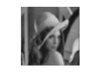
(b)

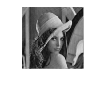
(c)

(d)

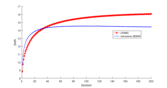
(e)

Fig. 1: Deblurring results for Lena under Gaussian operator by using the two algorithms. (a) Original image; (b) Blurred image; (c) IRPAMC 16.0dB; (d) nonconvex ADMM 14.4dB; (e) SNR versus the iterations.

4 Conclusion

In this paper, we propose an iteratively reweighted alternating minimization algorithm for a class of linearly constrained problems. The algorithm is developed from the perspective of penalty strategy. To speed up the iteration, we also employ a continuation trick for the penalty parameter. We prove the convergence of the algorithm under weaker assumptions than the nonconvex ADMM. Numerical results on the nonconvex TV deblurring problem are also presented for demonstrating the efficiency of the proposed algorithm.

References

- [1] Jonathan Eckstein and Wang Yao, “Understanding the convergence of the alternating direction method of multipliers: Theoretical and computational perspectives,” Pacific Journal of Optimization, vol. 11, no. 4, pp. 619–644, 2015.
- [2] Michel Fortin and Roland Glowinski, Augmented Lagrangian methods: applications to the numerical solution of boundary-value problems, Elsevier, 2000.
- [3] Daniel Gabay and Bertrand Mercier, “A dual algorithm for the solution of nonlinear variational problems via finite element approximation,” Computers & Mathematics with Applications, vol. 2, no. 1, pp. 17–40, 1976.
- [4] Roland Glowinski and JT Oden, “Numerical methods for nonlinear variational problems,” Journal of Applied Mechanics, vol. 52, pp. 739, 1985.
- [5] Yangyang Xu and Wotao Yin, “A block coordinate descent method for regularized multiconvex optimization with applications to nonnegative tensor factorization and completion,” SIAM Journal on imaging sciences, vol. 6, no. 3, pp. 1758–1789, 2013.
- [6] Yu Wang, Wotao Yin, and Jinshan Zeng, “Global convergence of ADMM in nonconvex nonsmooth optimization,” Journal of Scientific Computing, vol. 78, no. 1, pp. 29–63, 2015.
- [7] Mingyi Hong, Zhi-Quan Luo, and Meisam Razaviyayn, “Convergence analysis of alternating direction method of multipliers for a family of nonconvex problems,” SIAM Journal on Optimization, vol. 26, no. 1, pp. 337–364, 2016.
- [8] Fenghui Wang, Wenfei Cao, and Zongben Xu, “Convergence of multi-block Bregman ADMM for nonconvex composite problems,” Science China Information Sciences, vol. 61, no. 12, 122102, 2018.
- [9] Tao Sun, Hao Jiang, Lizhi Cheng, and Wei Zhu, “Iteratively linearized reweighted alternating direction method of multipliers for a class of nonconvex problems,” Transactons on Signal Processing, vol. 66, no. 20, pp. 5380–5391, 2018.
- [10] Amir Beck, “On the convergence of alternating minimization for convex programming with applications to iteratively reweighted least squares and decomposition schemes,” SIAM Journal on Optimization, vol. 25, no. 1, pp. 185–209, 2015.
- [11] Tao Sun and Lizhi Cheng, “Little- convergence rates for several alternating minimization methods,” Communications in Mathematical Sciences, vol. 15, no. 1, pp. 197–211, 2017.
- [12] Michael Hintermüler and Tao Wu, “Nonconvex TVq-models in image restoration: Analysis and a trust-region regularization–based superlinearly convergent solver,” SIAM Journal on Imaging Sciences, vol. 6, no. 3, pp. 1385–1415, 2013.
- [13] Rick Chartrand and Wotao Yin, “Iteratively reweighted algorithms for compressive sensing,” in Acoustics, speech and signal processing, IEEE international conference on, pp. 3869–3872, 2018.
- [14] Emmanuel J Candes, Michael B Wakin, and Stephen P Boyd, “Enhancing sparsity by reweighted minimization,” Journal of Fourier analysis and applications, vol. 14, no. 5, pp. 877–905, 2008.
- [15] Xiaojun Chen and Weijun Zhou, “Convergence of the reweighted minimization algorithm for minimization,” Computational Optimization and Applications, vol. 59, no. 1-2, pp. 47–61, 2014.
- [16] Tao Sun, Hao Jiang, and Lizhi Cheng, “Global convergence of proximal iteratively reweighted algorithm,” Journal of Global Optimization, vol. 68, no. 4, pp. 815–826, 2017.
- [17] Elaine T Hale, Wotao Yin, and Yin Zhang, “Fixed-point continuation for -minimization: Methodology and convergence,” SIAM Journal on Optimization, vol. 19, no. 3, pp. 1107–1130, 2008.
- [18] Tao Sun and Lizhi Cheng, “Convergence of iterative hard-thresholding algorithm with continuation,” Optimization Letters, vol. 11, no. 4, pp. 801–815, 2016.
- [19] Tao Sun, Hao Jiang, and Lizhi Cheng, “Hard thresholding pursuit with continuation for -regularized minimizations,” to be appeared in Mathematical Methods in the Applied Sciences.
- [20] Yilun Wang, Junfeng Yang, Wotao Yin, and Yin Zhang, “A new alternating minimization algorithm for total variation image reconstruction,” SIAM Journal on Imaging Sciences, vol. 1, no. 3, pp. 248–272, 2008.