Quantifying tensions in cosmological parameters:
Interpreting the DES evidence ratio

Abstract

We provide a new interpretation for the Bayes factor combination used in the Dark Energy Survey (DES) first year analysis to quantify the tension between the DES and Planck datasets. The ratio quantifies a Bayesian confidence in our ability to combine the datasets. This interpretation is prior-dependent, with wider prior widths boosting the confidence. We therefore propose that if there are any reasonable priors which reduce the confidence to below unity, then we cannot assert that the datasets are compatible. Computing the evidence ratios for the DES first year analysis and Planck, given that narrower priors drop the confidence to below unity, we conclude that DES and Planck are, in a Bayesian sense, incompatible under $\Lambda$CDM. Additionally we compute ratios which confirm the consensus that measurements of the acoustic scale by the Baryon Oscillation Spectroscopic Survey (BOSS) are compatible with Planck, whilst direct measurements of the acceleration rate of the Universe by the S$H_{0}$ES collaboration are not. We propose a modification to the Bayes ratio which removes the prior dependency using Kullback-Leibler divergences, and using this statistical test find Planck in strong tension with S$H_{0}$ES, in moderate tension with DES, and in no tension with BOSS. We propose this statistic as the optimal way to compare datasets, ahead of the next DES data releases, as well as future surveys. Finally, as an element of these calculations, we introduce in a cosmological setting the Bayesian model dimensionality, which is a parameterisation-independent measure of the number of parameters that a given dataset constrains.

I Introduction

The analysis of the first year of data from the Dark Energy Survey Abbott et al. (2018) (henceforth DES Y1) has generated considerable discussion. DES Y1 analysed data from cosmic shear, galaxy clustering, and galaxy-galaxy lensing (an analysis they refer to as “3x2” since it combines three two-point functions). This data combination is particularly suited to constraining the present day matter density $\Omega_{m}$ and the parameter $\sigma_{8}$, defined as the present-day linear theory root-mean-square amplitude of the power spectrum of matter fluctuations, averaged in spheres of radius $8h^{-1}{\rm Mpc}$, where $h$ is the Hubble constant in units of $100~{}{\rm km~{}s^{-1}~{}Mpc^{-1}}$. Before the publication of DES Y1, this parameter combination measured by weak lensing had already generated controversy, with claims of tensions with respect to the Cosmic Microwave Background (CMB) values measured by Planck Planck Collaboration (2018a) by both the CFHTLenS and Kilo Degree Survey (KiDS) collaborations Joudaki et al. (2017a); Köhlinger et al. (2017); Hildebrandt et al. (2017). Whilst this discrepancy has led to claims of new physics Joudaki et al. (2017b), it has also highlighted unknown problems in weak lensing analyses that have reduced these tensions to below significant levels Efstathiou and Lemos (2018); Troxel et al. (2018); Köhlinger et al. (2019).

DES Y1 obtained results that appear to be in mild tension with Planck (see Fig. 10 of DES Y1), but are reported to be perfectly consistent according to the evidence ratio statistic $R$ used in their analysis to quantify the degree of discordance between 3x2 and CMB data. Whilst this $R$ statistic was proposed some time ago Marshall et al. (2006), and supported since then by many cosmologists Trotta (2008); Verde et al. (2013a); Verde (2014); Raveri (2016); Seehars et al. (2016a), it is particularly relevant to consider its precise interpretation in light of present and future tensions arising with increasingly powerful datasets providing ever more precise parameter constraints. Other measures of tension between datasets have been proposed in the past Inman and Jr (1989); Battye et al. (2015); Seehars et al. (2014); Nicola et al. (2019); Kunz et al. (2006); Karpenka et al. (2015); MacCrann et al. (2015); Adhikari and Huterer (2019); Douspis et al. (2018); Raveri and Hu (2019). A summary of a lot of these methods can be found in Charnock et al. (2017).

In this paper we argue that $R$ is an appropriate measure of tension, quantifying the Bayesian degree of confidence in the ability to combine the data. However, $R$ has some subtle prior-dependent properties, which has led to its misuse in previous works. We explain these properties and provide Bayesian methods to correctly calibrate the scale on which it sits. We also propose an alternative statistic that preserves the desired properties of $R$ to compare different datasets, including its Bayesian nature, but does not suffer from undesired prior dependences.

The tension between weak galaxy lensing and Planck is not the only existing tension in cosmology. Measurements of the expansion rate of the Universe parameterised by the Hubble constant $H_{0}$ using Type Ia supernovae calibrated by the period-luminosity relation of Cepheids and local distance anchors by the S$H_{0}$ES collaboration Riess et al. (2016, 2018) are in tension with the Planck value inferred from the CMB using a $\Lambda{\rm CDM}$ cosmology Planck Collaboration (2018a). We use this case as an example of clear tension between experiments. Conversely, the measurements of the Baryon Acoustic Oscillation (BAO) scale and Redshift-Space Distortions (RSD) by BOSS Alam and et al. (2017) produce values of the parameters $\Omega_{m}$ and $\sigma_{8}$ that are in good agreement with Planck. We use this case as an example of no tension between experiments.

The paper is structured as follows: In Sec. II we briefly review the key Bayesian theory and establish notation. In Sec. III we define the logarithmic Bayes and information ratios $\log R$ and $\log I$ and present our new Bayesian interpretation of $\log R$. In Sec. IV we examine analytic examples to aid intuition on the properties of the Bayes and information ratios. In Sec. V we apply our techniques to cosmological datasets, with our key results reported in Tab. 2. We conclude in Sec. VI.

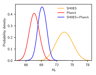
Figure 1: Tension between the S$H_{0}$ES and Planck datasets as exhibited by examining the posterior parameter constraints on the Hubble constant.

II Background

In general we use the following notation for the quantities in Bayes’ theorem:

$$P(\theta|D)=\frac{P(D|\theta)P(\theta)}{P(D)}\quad\Leftrightarrow\quad\mathcal{P}_{D}(\theta)=\frac{\mathcal{L}_{D}(\theta)\pi(\theta)}{\mathcal{Z}_{D}},$$

namely, the posterior $\mathcal{P}$, likelihood $\mathcal{L}$, prior $\pi$, and evidence $\mathcal{Z}$. We will retain dataset-dependence as a subscript, and in general will suppress explicit dependency on $\theta$ except where its presence increases clarity. Furthermore there is a suppressed explicit model dependence, which is taken to be $\Lambda$CDM for our cosmological examples.

II.1 Bayesian evidence

Throughout this paper the Bayesian evidence $\mathcal{Z}$, defined as

$$\mathcal{Z}_{D}=\int\mathcal{L}_{D}\pi\operatorname{d}\!{\theta},$$ (1)

will play a key role. Also known as the marginal likelihood Trotta (2008), the evidence is a key element of model comparison, and may be computed analytically in some rare cases, but is usually evaluated using a Laplace approximation MacKay (2002), Savage Dickey ratio Trotta (2007), or better still with numerical evidence calculators such as MCEvidence Heavens et al. (2017a, b) or nested sampling Skilling (2006); Feroz et al. (2009); Handley et al. (2015a, b); Brewer et al. (2011); Brewer and Foreman-Mackey (2016).

II.2 Kullback-Leibler divergence

The Kullback-Leibler divergence Kullback and Leibler (1951) is defined as

$$\mathcal{D}_{D}=\int\mathcal{P}_{D}(\theta)\log\frac{\mathcal{P}_{D}(\theta)}{\pi(\theta)}d{\theta}=\left\langle\log\frac{\mathcal{P}_{D}}{\pi}\right\rangle_{\mathcal{P}_{D},}$$ (2)

which quantifies the information gain/compression between prior and posterior and has been used by numerous authors Hosoya et al. (2004); Verde et al. (2013b); Seehars et al. (2014, 2016b); Grandis et al. (2016a); Raveri et al. (2016); Hee et al. (2016); Grandis et al. (2016b); Zhao et al. (2017); Nicola et al. (2017, 2019). The angular brackets $\langle f\rangle_{p}$ in the right-most expression of Eq. 2 denote the average of $f$ over the distribution $p$.

II.3 Bayesian model dimensionality

We define the Bayesian model dimensionality Handley and Lemos (2019) as

$$\frac{\tilde{d}_{D}}{2}=\left\langle{\left(\log\frac{\mathcal{P}_{D}}{\pi}\right)}^{2}\right\rangle_{\mathcal{P}_{D}}-\quad{\left\langle\log\frac{\mathcal{P}_{D}}{\pi}\right\rangle}_{\mathcal{P}_{D}.}^{2}$$ (3)

The quantity $\log[\mathcal{P}_{D}(\theta)/\pi(\theta)]$ is the Shannon information Shannon (1948) provided by the posterior relative to the prior at parameter $\theta$, measured in nats (natural bits). As can be seen from Eq. 2, the Kullback-Leibler divergence is the average amount of information provided by the posterior, whilst Eq. 3 shows that the Bayesian model dimensionality is proportional to the variance of the information provided by the posterior.

It should be noted that an earlier preprint of this paper used an alternative definition of the dimensionality by Spiegelhalter Spiegelhalter et al. (2002), which has several unattractive theoretical qualities when applied to significantly non-Gaussian cases. The fundamental qualitative conclusions remain unchanged from the initial version of this paper, and the newer definition of model dimensionality is examined in greater detail in Handley and Lemos (2019).

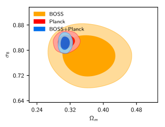
Figure 2: No tension between BOSS and Planck datasets as exhibited by examining the joint posterior parameter constraints on the matter fraction and $\sigma_{8}$.

II.4 Combining likelihoods

Independent datasets $A$ and $B$ are combined at the likelihood level via $\mathcal{L}_{AB}=\mathcal{L}_{A}\mathcal{L}_{B}$ so that

$$\mathcal{P}_{A}=\frac{\mathcal{L}_{A}\pi}{\mathcal{Z}_{A}},\quad\mathcal{P}_{B}=\frac{\mathcal{L}_{B}\pi}{\mathcal{Z}_{B}},\quad\mathcal{P}_{AB}=\frac{\mathcal{L}_{A}\mathcal{L}_{B}\pi}{\mathcal{Z}_{AB}}.$$ (4)

$$\mathcal{Z}_{A}=\int\mathcal{L}_{A}\pi\operatorname{d}\!{\theta},\quad\mathcal{Z}_{B}=\int\mathcal{L}_{B}\pi\operatorname{d}\!{\theta},$$

$$\mathcal{Z}_{AB}=\int\mathcal{L}_{A}\mathcal{L}_{B}\pi\operatorname{d}\!{\theta}.$$ (5)

In general, new datasets may introduce additional parameters, either because more cosmological parameters are constrained, or because additional nuisance parameters associated with foregrounds or instrumentation are required to perform inference. In general $\theta$ will be taken to be the span of the entire parameter space of interest.

An important point, often misunderstood by professional practitioners, is that the introduction of unconstrained parameters should not impact on proper inference. It is oft-quoted that Bayes factors (or equivalently evidences) penalise additional parameters, but in fact Bayes factors only penalise constrained parameters. For example, if one were to perform a model comparison between the six-parameter $\Lambda$CDM model and an extension to the model which factored in the age of the cosmologist doing the calculation, then both models would have the same evidence value, since a cosmologist’s age is (almost) completely unconstrained by cosmological likelihoods. This is not a bug, but a desirable feature of Bayes factors in their use in consistent inference. The proper Bayesian way to deal with this apparent problem is to exclude such trite models at the model prior level.

III The $R$ statistic

III.1 Definition and prior-dependence

Given two datasets $A$ and $B$, the $R$ statistic is defined via the equivalent expressions:

$$R=\frac{\mathcal{Z}_{AB}}{\mathcal{Z}_{A}\mathcal{Z}_{B}}=\frac{P(A,B)}{P(A)P(B)}=\frac{P(A|B)}{P(A)}=\frac{P(B|A)}{P(B)},$$ (6)

with all probabilities implicitly conditional on an underlying model (e.g. $\Lambda$CDM). A value of $R\gg 1$ is interpreted as both datasets being consistent, while $R\ll 1$ means the datasets are inconsistent. Note that whilst we assume that the datasets $A$ and $B$ are independent, this does not imply that $R=1$. Specifically, dataset independence means that likelihoods $\mathcal{L}_{D}(\theta)=P(D|\theta)$, which are probabilities conditioned on $\theta$, combine by multiplication, but evidences $\mathcal{Z}_{D}=P(D)$, which are likelihoods marginalised over the prior $\pi(\theta)=P(\theta)$, do not.

In the DES Y1 analysis, $R$ is used to quantify tension, with the Jeffreys’ scale used as the arbiter for whether models are consistent or not. The interpretation on a Jeffreys scale is somewhat unjustified, as the DES papers do not explain which probability ratio they are placing on the scale.

A second, arguably larger concern is that whilst $R$ satisfies many of desiderata that one would hope for from such a quantity (dimensional consistency, symmetry, parameterisation invariance, use of Bayesian quantities), it is strongly prior-dependent. We can render this dependency explicit by combining Eqs. 6, 5 and 4 to yield:

$$R=\int\frac{\mathcal{P}_{A}\mathcal{P}_{B}}{\pi}\operatorname{d}\!{\theta}=\left\langle\frac{\mathcal{P}_{B}}{\pi}\right\rangle_{\mathcal{P}_{A}}=\left\langle\frac{\mathcal{P}_{A}}{\pi}\right\rangle_{\mathcal{P}_{B}}.$$ (7)

Thus, $R$ can be thought of as the posterior average of the ratio of the other posterior to the shared prior. More specifically, $R$ depends on the priors set on constrained parameters shared between likelihoods, but not on the prior on additional nuisance or unconstrained parameters.

It should be noted that this variation is in opposition to the usual evidence prior-dependency. Namely, reducing the widths of the prior in general increases evidence. The same reduction of prior widths however will reduce the ratio $R$ and increase tension. This is easily understood, since in the $R$ ratio there are two evidences on the denominator with only one in the numerator. In a Bayesian sense this is an attractive balance—you can only evidence-hack at the expense of tension.

It is important to note that the prior dependence of $R$ can only hide existent discordance, i.e. $R$ can indicate that two datasets are in agreement, even when they are not. However, if $R$ indicates that two datasets are discordant, this should be taken seriously, since the prior volume effect only increases the value of $R$.

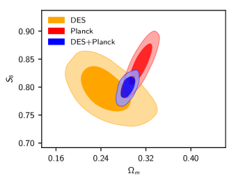
Figure 3: Possible tension between DES and Planck datasets as exhibited by examining the joint posterior parameter constraints on the matter fraction and the parameter combination $S_{8}=\sigma_{8}(\Omega_{m}/0.3)^{0.5}$.

III.2 Bayesian interpretation of $R$

An interpretation that is often posited is that $R$ represents a ratio of probabilities that the shared model parameters come from different universes in comparison with the probability that they come from the same universe. Given that evidences are traditionally used in the context of model comparison, this seems a natural interpretation. However, in order to convert evidences to model probabilities, one requires model priors and for probabilities to be conditioned on the same dataset, which in this case is not true. Raw evidences are probabilities of data, not of models.

A correct interpretation can be found by examining the two right-hand most expressions in Eq. 6. These expressions show that $R$ represents the relative confidence that we have in dataset $A$ in light of knowing dataset $B$, compared to the confidence in $A$ alone (and vice-versa). If $R>1$, then $B$ has strengthened our confidence in $A$ by a factor $R$. If $R\ll 1$, then as Bayesians we should be concerned that there is either a problem with the underlying model, or a problem with either or both of the datasets, and therefore avoid combining the two.

Given this interpretation, it is important to understand the prior-dependency of $R$, namely that decreasing the prior widths on shared parameters reduces our confidence in the ability to combine datasets.

If a Bayesian specifies extremely wide and uniform priors, they are saying that they a priori believe the parameter constraints derived from a dataset $D$ could reside anywhere within that region. It is therefore reassuring when two independent datasets result in constraints that are close. We should be proportionally more reassured if our initial prior were wider, as it is proportionally less likely a priori that they should lie close to one another.

Some practitioners might consider this prior dependency pathological, rather than the correct behaviour of such a probability. In our experience, the primary difference between full Bayesians and other statisticians is that a Bayesian considers this kind of prior-dependent behaviour of the analysis a feature rather than a bug.

Given this prior dependency and its sensible interpretation, the approach we advocate is as follows:

Proposition 1.

If there are any physically reasonable priors which render $R$ significantly less than 1, then as Bayesians we should consider these datasets in tension.

Given that narrowing the priors decreases the value of $R$, the physically reasonable priors that render the lowest possible value of $R$ are the narrowest priors that do not significantly alter the shape of the posteriors. Whilst such an extreme strategy would provide a definitive lower bound on $R$, many Bayesians would disagree with such a procedure, as it uses a prior that depends on the posterior. In reality, the most pragmatic approach is to choose reasonable initial priors, and then to examine the sensitivity of the conclusions to reasonable alterations to them.

III.3 Information and suspiciousness

The logarithmic version of Eq. 6 for the Bayes ratio in between two datasets $A$ and $B$ is defined as

$$\log R=\log\mathcal{Z}_{AB}-\log\mathcal{Z}_{A}-\log\mathcal{Z}_{B}.$$ (8)

As discussed in the previous section, the Bayesian confidence $R$ has two primary contributions, one from the unlikeliness of two datasets ever matching (proportional to prior), and another in their mismatch. We may quantify the first of these via the information ratio $I$ defined using Kullback-Leibler divergences as:

$$\log I=\mathcal{D}_{A}+\mathcal{D}_{B}-\mathcal{D}_{AB}.$$ (9)

The remaining part of the Bayesian confidence quantifies the mismatch, which we term the suspiciousness $S$:

$$\log S=\log R-\log I.$$ (10)

Suspiciousness is unaffected by changing the prior widths as long as this change does not significantly alter the posterior, since the information ratio $I$ and Bayes ratio $R$ transform similarly under prior volume alterations.

It is important to recognise that whilst $\log S$ is indeed prior-independent, in constructing this quantity we have lost the probabilistic interpretation found in $\log R$. More care must be taken to calibrate the scale on which $\log S$ sits, which will be considered at the end of the next section.

IV Analytical examples

In all of the below, for a graphical understanding, one may substitute $A$ $\leftrightarrow$ Planck, $B$ $\leftrightarrow$ S$H_{0}$ES, DES, or BOSS and consult Figs. 3, 1 and 2 respectively.

For simplicity, we consider $A$ and $B$ to have the same parameters $\theta$, although the case is easily extended to the case where the likelihoods only share some parameters, in which case our results depend only on those parameters that are shared between likelihoods.

IV.1 Top-hat example

As a simple choice, we consider a top-hat posterior over a multidimensional region $\mathcal{R}_{X}$, enclosing a volume $V_{X}$:

$$\mathcal{P}_{X}(\theta)=\left\{\begin{array}[]{cc}V_{X}^{-1}&:\theta\in\mathcal{R}_{X}\\ 0&:\text{otherwise}\end{array}\right.,\qquad V_{X}=\int_{\theta\in\mathcal{R}_{X}}\operatorname{d}\!{\theta}.$$ (11)

If we have a top-hat prior with volume $V_{\pi}$ enclosing two top-hat posteriors $P_{A}$ and $P_{B}$, along with their combined posterior $P_{AB}$, then

$$\log R=\log I=\log\frac{V_{AB}V_{\pi}}{V_{A}V_{B}}.$$ (12)

We can see the explicit prior dependency of $R$ with the presence of the $V_{\pi}$ term. Furthermore, we see that $R$ and $I$ are equal in the top-hat posterior, so that the entire contribution to $R$ is in information, and none in suspicion:

$$S=\left\{\begin{array}[]{cc}1&:\mathcal{R}_{A}\cap\mathcal{R}_{B}\neq\emptyset\\ 0&:\text{otherwise.}\end{array}\right.$$ (15)

Thus for the uniform case there is no suspiciousness, provided that the posteriors have any overlap region and are thus plausibly consistent.

IV.2 Gaussian example

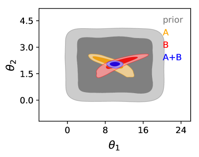
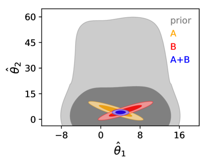
Figure 4: Many non-Gaussian posteriors (left) may be “Gaussianised” (right) by using Box-Cox transformations.

We now consider a less trivial multivariate Gaussian example Feeney et al. (2018, 2019). A $d$-dimensional Gaussian likelihood with peak $\mathcal{L}_{\mathrm{max}}$, centre $\mu$ and parameter covariance $\Sigma$, along with a top-hat enclosing prior over volume $V_{\pi}$ has likelihood, posterior, evidence and Kullback-Leibler divergence given by the following:

$$\log\mathcal{L}(\theta) =\log\mathcal{L}^{\mathrm{max}}-\frac{1}{2}(\theta-\mu)\Sigma^{-1}(\theta-\mu),$$ (16)

$$\log\mathcal{P}(\theta) =-\frac{1}{2}\log|2\pi\Sigma|-\frac{1}{2}(\theta-\mu)\Sigma^{-1}(\theta-\mu),$$ (17)

$$\log\mathcal{Z} =\log\mathcal{L}^{\mathrm{max}}+\frac{1}{2}\log|2\pi\Sigma|-\log V_{\pi},$$ (18)

$$\mathcal{D} =\log V_{\pi}-\frac{1}{2}(d+\log|2\pi\Sigma|).$$ (19)

Note that in the above we have removed explicit dimensionality-dependency from the normalisation of a Gaussian by exploiting the matrix determinant property $|2\pi\Sigma|={(2\pi)}^{d}|\Sigma|$.

Two likelihoods $A$ and $B$ combine using the relations

$$\log\mathcal{L}^{\mathrm{max}}_{AB}= -\frac{1}{2}(\mu_{A}-\mu_{B}){(\Sigma_{A}+\Sigma_{B})}^{-1}(\mu_{A}-\mu_{B})$$

$$+\log\mathcal{L}^{\mathrm{max}}_{A}+\log\mathcal{L}^{\mathrm{max}}_{B},$$ (20)

$$\Sigma_{AB}^{-1}= \Sigma_{A}^{-1}+\Sigma_{B}^{-1},$$ (21)

$$\mu_{AB}= \Sigma_{AB}\left[\Sigma_{A}^{-1}\mu_{A}+\Sigma_{B}^{-1}\mu_{B}\right].$$ (22)

It should also be noted that

$${(\Sigma_{A}+\Sigma_{B})}^{-1}=\Sigma_{A}^{-1}\Sigma_{AB}\Sigma_{B}^{-1}=\Sigma_{B}^{-1}\Sigma_{AB}\Sigma_{A}^{-1}.$$ (23)

We therefore find

$$\log R= -\frac{1}{2}(\mu_{A}-\mu_{B}){(\Sigma_{A}+\Sigma_{B})}^{-1}(\mu_{A}-\mu_{B})$$

$$-\frac{1}{2}\log\left|2\pi(\Sigma_{A}+\Sigma_{B})\right|+\log V_{\pi},$$ (24)

and

$$\log I= -\frac{d}{2}-\frac{1}{2}\log\left|2\pi(\Sigma_{A}+\Sigma_{B})\right|+\log V_{\pi}.$$ (25)

We thus find the information content can be used to remove all of the residual prior dependence from $\log R$, giving a suspiciousness:

$$\log S=\frac{d}{2}-\frac{1}{2}(\mu_{A}-\mu_{B}){(\Sigma_{A}+\Sigma_{B})}^{-1}(\mu_{A}-\mu_{B}).$$ (26)

The numerical value of the suspiciousness is determined by the means and covariances of the posterior distributions $A$ and $B$. Under a Bayesian interpretation of the posterior, if the “true” value of the measured parameter is $\theta_{0}$, then both means are drawn from a normal distribution centred on this value with covariance equal to their posterior covariance $\mu_{A}\sim\mathcal{N}(\theta_{0},\Sigma_{A})$, $\mu_{B}\sim\mathcal{N}(\theta_{0},\Sigma_{B})$, and their difference is drawn from a distribution centred on zero with covariance equal to the sum of the underlying covariances $\mu_{A}-\mu_{B}\sim\mathcal{N}(0,\Sigma_{A}+\Sigma_{B})$. One can see that $d-2\log S$, has a $\chi^{2}_{d}$ distribution, and that $\log S$ is typically $0\pm\sqrt{d/2}$. An overly negative value of $\log S$ indicates discordance, and an overly positive value suspicious concordance. More quantitatively, one can use the inverse cumulative $\chi^{2}_{d}$ distribution to turn $\log S$ into the tension probability of two datasets being this discordant by chance:

$$p=\int\limits_{d-2\log S}^{\infty}\chi^{2}_{d}(x)\operatorname{d}\!{x}=\int\limits_{d-2\log S}^{\infty}\frac{x^{d/2-1}e^{-x/2}}{2^{d/2}\Gamma(d/2)}\operatorname{d}\!{x}.$$ (27)

Whilst this procedure is only exact for the Gaussian case, a reasonable proposition for general posteriors would be to compute $\log S$ numerically, and then determine tension via a $\chi^{2}$-like test, in analogy with the Gaussian case:

Proposition 2.

If $p\lesssim 0.05$, where $p$ is the tension probability computed from Eq. 27, $\log S$ is computed using numerical evidences and Kullback-Leibler divergences, and $d=\tilde{d}_{A}+\tilde{d}_{B}-\tilde{d}_{AB}$ is the Bayesian model dimensionality of the shared constrained parameters computed using Eq. 3, then the datasets should be considered in moderate tension. If $p\lesssim 0.003$, they should be considered in strong tension.

For the case when the posteriors are exactly (or extremely close to) Gaussian, the tension probability $p$ may be interpreted as a probability that one would observe such a discrepancy by chance alone. In the non-Gaussian case, $p$ is only a rough calibration so only extremely small values of $p$ should be regarded with suspicion. The suspiciousness $S$ can be used to determine discordance if $S\ll-\sqrt{\tilde{d}/2}$, and the tension probability $p$ provides a mechanism for putting a number on the concept of $\ll$ in this case. The $R$ statistic, however, is always interpretable as a Bayesian confidence in our ability to combine the data, irrespective of Gaussianity.

It should be noted that many posteriors may be “Gaussianised” using techniques like Box-Cox transformations Box and Cox (1964). These transformations are non-linear mappings that can transform complex posteriors into approximately Gaussian ones by changing the parameterization, and have already been used in the context of cosmology Joachimi and Taylor (2011); Schuhmann et al. (2016). It can be easily proven that these transformations preserve the value of the suspiciousness, although care must be taken to also transform the underlying common prior distribution appropriately (Fig. 4), and that the prior is not significantly distorted by the Box-Cox transformation in the region of the posterior bulk.

Our two propositions for tension quantification are in fact related: one can think of $\log I$ as being the volume of the narrowest prior that does not significantly impinge upon the posterior bulk, and Proposition 2 is one method for quantifying the qualitative statement “any reasonable prior” in Proposition 1. Finally, the interpretation of the Bayesian model dimensionality $\tilde{d}_{D}$ as the effective number of parameters is made clear in the Gaussian case, since $\tilde{d}_{D}=d$.

V Numerical examples

Prior	S$H_{0}$ES	BOSS	DES	Planck	S$H_{0}$ES+Planck	BOSS+Planck	DES+Planck
default	$0.93\pm 0.03$	$2.95\pm 0.07$	$14.01\pm 0.32$	$15.84\pm 0.38$	$15.98\pm 0.37$	$15.89\pm 0.36$	$25.89\pm 0.63$
medium	$0.98\pm 0.03$	$3.79\pm 0.09$	$13.35\pm 0.31$	$15.89\pm 0.38$	$15.09\pm 0.35$	$16.38\pm 0.37$	$26.10\pm 0.65$
narrow	$1.68\pm 0.03$	$1.40\pm 0.02$	$10.89\pm 0.24$	$15.96\pm 0.37$	$15.72\pm 0.37$	$15.69\pm 0.37$	$25.69\pm 0.62$

Table 1: Bayesian model dimensionality of $\Lambda$CDM for all datasets and priors considered in this paper, calculated using Eq. 3.

Dataset	Prior	$\hfill\log R\hfill$	$\hfill\log I\hfill$	$\hfill\log S\hfill$	$\hfill\tilde{d}\hfill$	$\hfill p(\%)\hfill$
BOSS-Planck	default	$6.30\pm 0.29$	$6.18\pm 0.29$	$0.11\pm 0.11$	$2.91\pm 0.51$	$42.66\pm 4.28$
	medium	$4.51\pm 0.28$	$4.06\pm 0.28$	$0.46\pm 0.12$	$3.30\pm 0.55$	$55.12\pm 4.47$
	narrow	$1.30\pm 0.23$	$0.69\pm 0.22$	$0.61\pm 0.12$	$1.67\pm 0.54$	$77.12\pm 14.10$
DES-Planck	default	$2.88\pm 0.35$	$6.15\pm 0.34$	$-3.28\pm 0.16$	$3.97\pm 0.82$	$3.23\pm 1.00$
	medium	$0.51\pm 0.34$	$4.00\pm 0.34$	$-3.49\pm 0.16$	$3.13\pm 0.81$	$2.04\pm 0.79$
	narrow	$-1.88\pm 0.29$	$0.90\pm 0.29$	$-2.78\pm 0.16$	$1.15\pm 0.77$	$1.44\pm 0.91$
S$H_{0}$ES-Planck	default	$-2.03\pm 0.29$	$1.96\pm 0.28$	$-3.99\pm 0.12$	$0.78\pm 0.52$	$0.25\pm 0.17$
	medium	$-2.50\pm 0.28$	$1.56\pm 0.28$	$-4.06\pm 0.11$	$1.77\pm 0.51$	$0.56\pm 0.24$
	narrow	$-2.00\pm 0.23$	$1.43\pm 0.23$	$-3.43\pm 0.12$	$1.92\pm 0.52$	$1.17\pm 0.45$

Table 2: Comparison statistics. The values of $\log R$ and $\log I$ are computed via Eqs. 8 and 9, using the evidences and Kullback-Leibler divergences reported in Fig. 5. The suspiciousness statistic is simply $\log S=\log R-\log I$. $\tilde{d}$ is the Bayesian combined model dimensionality from Eq. 3, detailing the number of shared constrained parameters between the datasets, and $p$ is the tension probability computed from Eq. 27. One can see explicitly the prior dependency of $\log R$ and $\log I$, and how this is removed/reduced in $\log S$ and $p$. In both the Bayes ratio $\log R$ via Proposition 1 and the tension probability $p$ via Proposition 2, we find that the data show no tension between BOSS-Planck, moderate discordance between DES-Planck, and strong discordance between S$H_{0}$ES-Planck.

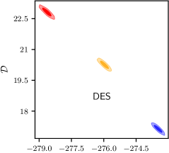
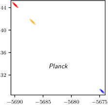
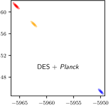
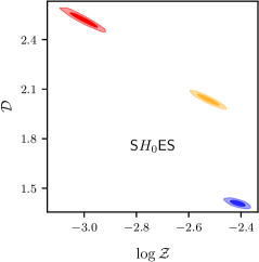
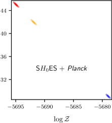
Figure 5: Log-evidence $\log\mathcal{Z}$ and Kullback-Leibler divergence $\mathcal{D}$ calculations for all datasets and priors considered in this paper. The figures show the numerical values for the log-evidence and Kullback-Leibler divergence for the likelihoods described in Sec. V.2 under the default and narrow priors summarised in Fig. 6, with red representing results for the default priors, orange medium priors and blue narrow priors. One can see that narrowing the prior increases the log-evidence and reduces the Kullback-Leibler divergence, but that $\log\mathcal{Z}+\mathcal{D}$ remains constant to within error. It should also be noted that the errors in estimating $\log\mathcal{Z}$ and $\mathcal{D}$ are strongly correlated. These errors arise from the uncertainty inherent in nested sampling’s estimate of the volume compression of each likelihood contour, and influences both quantities in the same manner. It should be noted that the parameter combination that we are most interested in estimating ($\log\mathcal{Z}+\mathcal{D}$) has the lowest error in its estimation.

We now apply our techniques to the cosmological dataset pairings of Cosmic Microwave Background data (CMB) with Baryon Acoustic Oscillations plus Redshift-Space Distortions (BAO+RSD), galaxy clustering and weak lensing (3x2), and supernovae (SNe) respectively. This necessitates the numerical computation of evidences and Kullback-Leibler divergences via nested sampling. We find that BAO+RSD observations are fully consistent with CMB, 3x2 is in moderate tension, and SNe are in strong tension. Our results are summarised in Tab. 2.

V.1 Nested sampling computation

To compute the log-evidence $\log\mathcal{Z}$ and the Kullback-Leibler divergence $\mathcal{D}$ we use the outputs of a nested sampling run produced by CosmoChord Handley (2019), a modified version of CosmoMC Lewis and Bridle (2002) using PolyChord Handley et al. (2015a, b) as a nested sampler. For a reliable computation of evidences and Kullback-Leibler divergences, we found it essential to use PolyChord rather than MultiNest Feroz et al. (2009), due to the high dimensionality of the space of cosmological and nuisance parameters. Furthermore, PolyChord is able to dramatically speed up nested sampling in the context of cosmology by utilizing the fast-slow hierarchy between nuisance and cosmological parameters Lewis (2013). As a historical note, PolyChord was invented as an alternative to MultiNest in the context of the Planck collaboration Planck Collaboration (2016a, 2018b) to resolve precisely the issues described above.

The log-evidences and KL divergences are computed using the likelihood contours $\mathcal{L}_{i}$ of the discarded points from the trapezoidal rule

$$\mathcal{Z}\approx \sum_{i=1}^{N}\mathcal{L}_{i}\times\frac{1}{2}(X_{i-1}-X_{i+1}),$$

$$\mathcal{D}\approx \sum_{i=1}^{N}\frac{\mathcal{L}_{i}}{\mathcal{Z}}\log\frac{\mathcal{L}_{i}}{\mathcal{Z}}\times\frac{1}{2}(X_{i-1}-X_{i+1}),$$

$$\frac{\tilde{d}}{2}\approx \sum_{i=1}^{N}{\frac{\mathcal{L}_{i}}{\mathcal{Z}}\left(\log\frac{\mathcal{L}_{i}}{\mathcal{Z}}-\mathcal{D}\right)}^{2}\times\frac{1}{2}(X_{i-1}-X_{i+1}),$$

$$X_{i}= t_{i}X_{i-1},\qquad X_{0}=1,\qquad X_{N+1}=0,$$ (28)

where $X_{i}$ are the prior volumes of the $N$ likelihood contours and the $t_{i}$ are real random variables with probability distribution function:

$$P(t_{i})=n_{i}t_{i}^{n_{i}-1}\>[0<t_{i}<1]$$ (29)

Here $n_{i}$ are the (usually constant) number of active live points enclosed by each likelihood contour $\mathcal{L}_{i}$. To account for all of the correlation between the random variables $\mathcal{D}$ and $\log\mathcal{Z}$, we simulate a set of weights $\{t_{i}\}$ using Eq. 29, and compute $\mathcal{Z}$, $\mathcal{D}$ and $\tilde{d}$ from Eq. 28 using the same weights. This process is repeated 1000 times to build up a set of samples from the $P(\mathcal{Z},\mathcal{D},\tilde{d})$ distribution. Examples of such distributions can be seen graphically in Fig. 5. The log-sum-exp trick must be carefully utilized to avoid overflow errors throughout these computations. For more detail, consult John Skilling’s original nested sampling paper Skilling (2006). Code to compute these quantities is now publicly available as part of the anesthetic pip-installable Python package Handley (2019).

For our final runs, we used the CosmoChord settings $n_{\mathrm{live}}=1000$, $n_{\mathrm{prior}}=10000$, with all other settings left at their defaults for version 1.15. It is worth remarking that run-time is linear in the number of live points, and that PolyChord (in contrast to MultiNest) can function with extremely low numbers of live points. For low-resolution testing purposes $n_{\mathrm{live}}$ can be set as low as 10, which proves invaluable in the initial exploratory stages of a project when publication-quality runs are not essential.

V.2 Cosmological Likelihoods

For CMB observations we use the publicly available Planck 2015 TT+lowl+lowTEB likelihoods  Planck Collaboration (2016d). For BAO+RSD observations we use the 6DF+MGS BOSS DR12 final consensus data Alam and et al. (2017); Beutler et al. (2011); Ross et al. (2015). For 3x2 data, we use the 1 year final DES dataset Abbott et al. (2018). Finally, for SNe data we use a Gaussian likelihood on the Hubble parameter with mean and width indicated by the latest S$H_{0}$ES constraints Riess et al. (2018).

We follow the notation and parameterisation detailed in the respective likelihood papers, and we direct readers to those for further information on the meaning and notation of parameters.

V.3 Priors

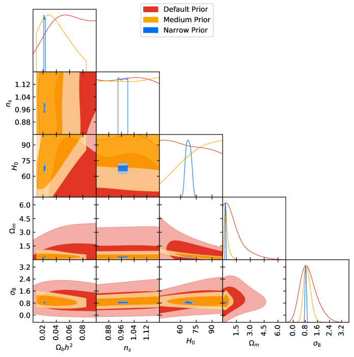
Parameter Default prior Medium prior Narrow prior $\Omega_{b}h^{2}$ $[0.005,0.1]$ $[0.01,0.085]$ $[0.0211,0.0235]$ $\Omega_{c}h^{2}$ $[0.001,0.99]$ $[0.08,0.21]$ $[0.108,0.131]$ $100\theta_{MC}$ $[0.5,10]$ $[0.97,1.5]$ $[1.038,1.044]$ $\tau$ $[0.01,0.8]$ $[0.01,0.8]$ $[0.01,0.16]$ $n_{s}$ $[0.8,1.2]$ $[0.8,1.2]$ $[0.938,1]$ $\ln(10^{10}A_{s})$ $[1.61,3.91]$ $[2.6,3.8]$ $[2.95,3.25]$

Figure 6: The three priors used throughout Sec. V. The priors provided to CosmoMC are shown in the upper-right table. These construct an approximate box-prior on the six cosmological parameters. Two of the cosmological parameters are shown in the triangle plot, and indeed a box prior can be seen on the $n_{s}$ parameter. The $\Omega_{b}h^{2}$ prior is not a simple top-hat prior on account of the fact that CosmoMC discards unphysical parameter combinations at the prior level. The remaining parameters are “derived parameters” and in general will not have box-priors, as can be seen in the $(H_{0},\Omega_{b}h^{2})$ plot.

To demonstrate the prior dependencies of $\log R$ and $\log S$, we choose three priors. The first is the default prior provided by CosmoMC. Note that this prior is not a trivial top-hat box prior, since CosmoMC places a model-dependent prior on the parameter space by eliminating regions that are unphysical. This non-trivial shape is shown in Fig. 6. We compare the default with two alternative prior choices; a “narrow” box centred on the posterior mean of Planck, with widths extending to 5$\sigma$ of the Planck posterior, and a “medium” box designed to encompass the DES posterior whilst being a little narrower than the default. The narrow prior is arguably rather tight, but is chosen as the other extreme end of prior choice from the default prior to emphasise the prior dependency of the $R$ statistic. It is worth noting that there is nothing particularly special about the choice of prior provided by the CosmoMC default, which could easily be narrowed or widened without a great deal of consensus objection.

V.4 Posteriors

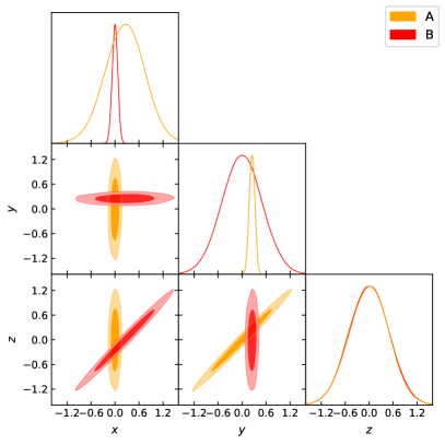
Figure 7: Hidden tension in a multivariate Gaussian. By eye, the three-dimensional posterior on the left seems to be in reasonable agreement. The one- and two-dimensional marginalised posteriors are clearly consistent. However, upon making the linear transformation indicated on the right, it is clear that the posteriors are in fact disjoint. Such issues become harder in higher-dimensional posteriors, and demonstrate the importance of a parameterisation-independent measures of tension such as those that we demonstrate here.

The posterior on the Hubble parameter for S$H_{0}$ES and Planck produced by PolyChord is shown in Fig. 1. By eye it is clear from the individual posteriors that the inferences on the value of $H_{0}$ are incompatible, and that the combined posterior cannot be trusted.

For BOSS and Planck, we show the marginalised posterior on the two parameters $\sigma_{8}$ and $\Omega_{m}$ in Fig. 2. Here there is significant overlap between the two-dimensional marginalised posteriors, and the combined posterior is valid. Note that they do not lie precisely on top on each other, which is in itself reassuring as otherwise the datasets would be suspiciously in agreement (and would usually indicate an overestimate of the errors or biases in the analysis).

For DES and Planck, we show the marginalised posterior for two parameters similar to those used in the BOSS case. In this case the situation is less clear, with a large proportion of the marginalised posterior bulk in disagreement, but with a small degree of overlap. If one looks at other parameter combinations, the tension becomes better or worse, and indeed it is possible to consider situations where there appears to be excellent overlap in every pair of parameters. However, it should be noted that since tension is a parameter invariant notion, if one can resolve a significant tension in any parameter combination, then this indicates significant discordance that cannot be removed. A toy example of such a posterior is shown in Fig. 7. The advantage of building a general dimensional parameterisation-independent prescription to quantify tension is that one can detect discrepancies even if none of the traditional parameters show obvious tension in their marginalised plots.

V.5 Evidences and Kullback-Leibler divergences

The numerical evidences and Kullback-Leibler divergences computed from runs produced by PolyChord using the technique described in Sec. V.1 are reported in Fig. 5.

The first thing to note is that nested sampling does not produce an exact value for the evidence and KL divergence, but instead produces a correlated probability distribution. The correlation is negative, since the dominant error in the evidence estimate is associated with the cumulative Poisson noise in estimating the prior volume contraction at each iteration, and this error contributes equally to both the evidence and KL estimates. Note however that this is advantageous when we wish to compute the $\log S$ ratio, since the error is minimal for the parameters contribution $\log\mathcal{Z}+\mathcal{D}$, as these prior volume errors cancel out to a large extent.

The second observation that should be made is that as we adjust the priors, the log-evidences increase as the normalisation of the prior changes, the Kullback-Leibler divergences decrease since there is less compression between prior and posterior, but the combination $\log\mathcal{Z}+\mathcal{D}$ remains approximately constant.

V.6 Bayesian model dimensionalities

The Bayesian model dimensionality for $\Lambda$CDM is detailed for each dataset and prior in Tab. 1. As this is the first time such quantities have been utilised in a cosmological setting, they are worthy of some discussion.

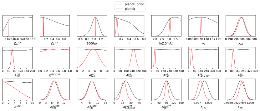
Figure 8: One-dimensional marginalised default prior (black) and Planck posterior (red). The Bayesian model dimensionality of $\tilde{d}_{\textit{Planck}}\approx 16$ is reflected by the fact that only a subset of the nuisance parameters are constrained by the data.

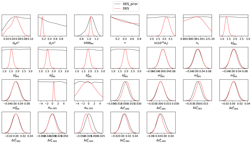
Figure 9: One-dimensional marginalised default prior (black) and DES Y1 posterior (red). The Bayesian model dimensionality of $\tilde{d}_{\mathrm{DES}}\approx 14$ is reflected by the fact that only a combination of the cosmological parameters and a subset of the nuisance parameters are constrained by the data.

First, the model dimensionality of the Planck dataset remains stable at $\tilde{d}_{\textit{Planck}}{}\approx 15$ for all priors. Whilst the Planck 2015 temperature likelihoods nominally have 21 parameters (6 cosmological and 15 nuisance), only a subset of the nuisance parameters are constrained by the data, as can be seen in Fig. 8. The fact that this dimensionality remains constant for all prior choices is due to the fact that the priors enclose the Planck posterior bulk in all three cases.

Second, in analogy with Planck, the DES Y1 data have a dimensionality of $\tilde{d}_{\mathrm{DES{}}}\approx 11$. As can be seen in Fig. 9, most of the 20 nuisance parameters and some of the 6 cosmological parameters are unconstrained. Quantifying the dimensionality in this case is made yet harder by the fact that unlike Planck, the DES Y1 survey best constrains a non-trivial combination of the sampled parameters, (e.g. $\sigma_{8}$). It is for this reason that it is essential to have a parameterisation-independent measure of the dimensionality of the constrained parameter space, such as that provided by the Bayesian model dimensionality. Additionally, unlike Planck, for DES there is a slight prior-dependence of the dimensionality for the narrow priors. This can be understood by the fact that the narrow priors cut a little into the DES posterior, effectively rendering some parameters less constrained relative to the wider prior.

This prior dependency is also mirrored in the S$H_{0}$ES and BOSS datasets, although less trivially. For default and medium priors, the dimensionality $\tilde{d}_{\mathrm{S}H_{0}\mathrm{ES}}=1$ reproduces the correct dimensionality given that the likelihood is only a Gaussian on the Hubble parameter. The fact that this rises to $\tilde{d}_{\mathrm{S}H_{0}\mathrm{ES}}=2$ for the narrow prior is as a result of a non-trivial degeneracy that emerges for narrow priors in the combination of $(H_{0},\Omega_{c}h^{2})$, meaning that the tension constraint of S$H_{0}$ES generates an artificial constraint on $\Omega_{c}h^{2}$. The dimensionality of BOSS is yet more complicated, but consistent with the degeneracies between its likelihood and our prior choice.

Finally the combined dimensionalities $\tilde{d}=\tilde{d}_{A}+\tilde{d}_{B}-\tilde{d}_{AB}$ are detailed in the penultimate column of Tab. 2. These show the number of constrained parameters that the datasets have in common, and we can see that DES and Planck share between 1 and $2.5$ constrained parameters depending on the prior chosen.

In conclusion, there is a rich structure in Bayesian model dimensionalities, and it is our hope that Bayesian model dimensionality becomes more widely used in cosmological inference.

V.7 Ratios

We present our key numerical results for the Bayes ratio $R$ and tension probabilities $p$ in Tab. 2.

First, we find that $\log R>0$ for all priors considered for the BOSS+Planck combination, indicating that BAO+RSD datasets are consistent with CMB. More precisely, knowledge of the BOSS dataset boosts our probabilistic confidence in the CMB data by a factor $\sim 500$ for the default priors, or $\sim 16$ for the narrow priors. We find that $\log S$ is positive and around zero, with a corresponding tension probability $p\gg 5\%$. One should note that $\log S$ and $p$ are not quite prior-independent since the narrowed priors impinge somewhat on the posterior bulk of the BOSS dataset.

Second for S$H_{0}$ES+Planck, we find that $\log R<0$ for all priors, with our confidence in CMB data dropping in light of knowing the SNe data for all choices of prior, indicating inconsistency. This is also reflected in the tension probabilities, which indicate $p\sim 0.3\%$ probability of getting such inconsistency by chance.

Finally, for DES data, the default priors show $R\sim 20$, whilst the narrow priors give $R\sim 0.1$. Under Proposition 1, given that there are some priors which indicate a reduction in confidence in CMB data in light of 3x2 data, we should therefore not regard the datasets as being consistent. Considering the tension statistic, there is a roughly $2\%$ probability of getting such an inconsistency by chance alone. We would therefore consider DES data to be in moderate tension with Planck.

V.8 Comparison with the DES analysis

It should be noted that our conclusion of moderate tension between DES and Planck is in contradiction to that presented in DES Y1. In DES Y1, they compute $R=2.8$, and therefore conclude that there is no tension with CMB data, and hence the datasets are safe to use in conjunction with one another. Aside from a consideration of the precise meaning of $R$, which is the focus of the first three sections of this paper, there are several issues with their analysis. First, they do not report the errors arising from computing this quantity via nested sampling. Given that they in general use similar settings to ours, it is conceivable that their value of $2.8$ is close to being consistent with $R=1$. Second they use MultiNest to compute this statistic, which renders the value of $R$ that they compute unreliable. Third, they give no consideration to the prior dependency of the $R$ statistic, or to the fact that a small adjustment to their priors would have generated $R<1$. Whilst this dependency is undesirable for some analysts, it should be noted that consistent datasets (e.g. BOSS and Planck) in general should have $R\gg 1$, independent of prior choice.

VI Conclusion

In this paper, we examined the Bayes ratio statistic used by DES to quantify the tension between potentially discordant datasets. We provided a novel interpretation of this statistic as a Bayesian quantification of our confidence in our ability to combine the datasets. It represents the factor by which our degree of belief in a dataset is strengthened in light of having incorporated the information provided by another dataset. We explain why this number is prior dependent, and under Proposition 1 say that if there is any reasonable prior choice which brings the factor to less than unity, then the datasets should be considered discordant.

For those who mislike the prior dependency of the Bayes ratio, we provide a method of calibrating the statistic using Kullback-Leibler divergences. Inspired by the Gaussian case, Proposition 2 provides a Bayesian tension probability, akin to the frequentist $p$-value statistic. As discussed in the introduction, there are several alternative methods for quantifying tensions in the literature, but we claim that this is the only method that preserves all the desiderata of the Bayes ratio, whilst remaining insensitive to prior volume effects.

We applied these new techniques and interpretations to CMB data from Planck combined with the 3x2 data from DES, the BAO+RSD data from BOSS or the SNe data from S$H_{0}$ES. Our technique confirms the consensus view that in comparison with the CMB, there is strong tension with SNe, moderate tension with 3x2 and no tension with BAO+RSD.

We believe that the $R$ statistic is a valuable one for the community to use to compute tension between datasets, but that care must be taken with its interpretation. We hope that these considerations will be taken into account in future DES releases.

References

- Abbott et al. [2018] T. M. C. Abbott, F. B. Abdalla, A. Alarcon, J. Aleksić, S. Allam, S. Allen, A. Amara, J. Annis, J. Asorey, S. Avila, and et al. Dark Energy Survey year 1 results: Cosmological constraints from galaxy clustering and weak lensing. Phys. Rev. D, 98(4):043526, Aug 2018. doi: 10.1103/PhysRevD.98.043526.
- Planck Collaboration [2018a] Planck Collaboration. Planck 2018 results. VI. Cosmological parameters. arXiv e-prints, art. arXiv:1807.06209, July 2018a.
- Joudaki et al. [2017a] Shahab Joudaki, Chris Blake, Catherine Heymans, Ami Choi, Joachim Harnois-Deraps, Hendrik Hildebrandt, Benjamin Joachimi, Andrew Johnson, Alexander Mead, David Parkinson, Massimo Viola, and Ludovic van Waerbeke. CFHTLenS revisited: assessing concordance with Planck including astrophysical systematics. MNRAS, 465:2033–2052, February 2017a. doi: 10.1093/mnras/stw2665.
- Köhlinger et al. [2017] F. Köhlinger, M. Viola, B. Joachimi, H. Hoekstra, E. van Uitert, H. Hildebrandt, A. Choi, T. Erben, C. Heymans, S. Joudaki, D. Klaes, K. Kuijken, J. Merten, L. Miller, P. Schneider, and E. A. Valentijn. KiDS-450: the tomographic weak lensing power spectrum and constraints on cosmological parameters. MNRAS, 471:4412–4435, November 2017. doi: 10.1093/mnras/stx1820.
- Hildebrandt et al. [2017] H. Hildebrandt, M. Viola, C. Heymans, S. Joudaki, K. Kuijken, C. Blake, T. Erben, B. Joachimi, D. Klaes, L. Miller, C. B. Morrison, R. Nakajima, G. Verdoes Kleijn, A. Amon, A. Choi, G. Covone, J. T. A. de Jong, A. Dvornik, I. Fenech Conti, A. Grado, J. Harnois-Déraps, R. Herbonnet, H. Hoekstra, F. Köhlinger, J. McFarland, A. Mead, J. Merten, N. Napolitano, J. A. Peacock, M. Radovich, P. Schneider, P. Simon, E. A. Valentijn, J. L. van den Busch, E. van Uitert, and L. Van Waerbeke. KiDS-450: cosmological parameter constraints from tomographic weak gravitational lensing. MNRAS, 465:1454–1498, February 2017. doi: 10.1093/mnras/stw2805.
- Joudaki et al. [2017b] Shahab Joudaki, Alexander Mead, Chris Blake, Ami Choi, Jelte de Jong, Thomas Erben, Ian Fenech Conti, Ricardo Herbonnet, Catherine Heymans, Hendrik Hildebrandt, Henk Hoekstra, Benjamin Joachimi, Dominik Klaes, Fabian Köhlinger, Konrad Kuijken, John McFarland, Lance Miller, Peter Schneider, and Massimo Viola. KiDS-450: testing extensions to the standard cosmological model. MNRAS, 471:1259–1279, October 2017b. doi: 10.1093/mnras/stx998.
- Efstathiou and Lemos [2018] George Efstathiou and Pablo Lemos. Statistical inconsistencies in the KiDS-450 data set. MNRAS, 476:151–157, May 2018. doi: 10.1093/mnras/sty099.
- Troxel et al. [2018] M. A. Troxel, E. Krause, C. Chang, T. F. Eifler, O. Friedrich, D. Gruen, N. MacCrann, A. Chen, C. Davis, J. DeRose, S. Dodelson, M. Gatti, B. Hoyle, D. Huterer, M. Jarvis, F. Lacasa, P. Lemos, H. V. Peiris, J. Prat, S. Samuroff, C. Sánchez, E. Sheldon, P. Vielzeuf, M. Wang, J. Zuntz, O. Lahav, F. B. Abdalla, S. Allam, J. Annis, S. Avila, E. Bertin, D. Brooks, D. L. Burke, A. Carnero Rosell, M. Carrasco Kind, J. Carretero, M. Crocce, C. E. Cunha, C. B. D’Andrea, L. N. da Costa, J. De Vicente, H. T. Diehl, P. Doel, A. E. Evrard, B. Flaugher, P. Fosalba, J. Frieman, J. García-Bellido, E. Gaztanaga, D. W. Gerdes, R. A. Gruendl, J. Gschwend, G. Gutierrez, W. G. Hartley, D. L. Hollowood, K. Honscheid, D. J. James, D. Kirk, K. Kuehn, N. Kuropatkin, T. S. Li, M. Lima, M. March, F. Menanteau, R. Miquel, J. J. Mohr, R. L. C. Ogando, A. A. Plazas, A. Roodman, E. Sanchez, V. Scarpine, R. Schindler, I. Sevilla-Noarbe, M. Smith, M. Soares-Santos, F. Sobreira, E. Suchyta, M. E. C. Swanson, D. Thomas, A. R. Walker, and R. H. Wechsler. Survey geometry and the internal consistency of recent cosmic shear measurements. MNRAS, 479:4998–5004, October 2018. doi: 10.1093/mnras/sty1889.
- Köhlinger et al. [2019] Fabian Köhlinger, Benjamin Joachimi, Marika Asgari, Massimo Viola, Shahab Joudaki, and Tilman Tröster. A Bayesian quantification of consistency in correlated data sets. MNRAS, 484(3):3126–3153, Apr 2019. doi: 10.1093/mnras/stz132.
- Marshall et al. [2006] Phil Marshall, Nutan Rajguru, and Anže Slosar. Bayesian evidence as a tool for comparing datasets. Phys. Rev. D, 73:067302, March 2006. doi: 10.1103/PhysRevD.73.067302.
- Trotta [2008] R. Trotta. Bayes in the sky: Bayesian inference and model selection in cosmology. Contemporary Physics, 49:71–104, March 2008. doi: 10.1080/00107510802066753.
- Verde et al. [2013a] Licia Verde, Pavlos Protopapas, and Raul Jimenez. Planck and the local Universe: Quantifying the tension. Physics of the Dark Universe, 2:166–175, September 2013a. doi: 10.1016/j.dark.2013.09.002.
- Verde [2014] Licia Verde. Precision cosmology, accuracy cosmology and statistical cosmology. Proceedings of the International Astronomical Union, 10(S306):223–234, 2014. doi: 10.1017/S1743921314013593.
- Raveri [2016] M. Raveri. Are cosmological data sets consistent with each other within the cold dark matter model? Phys. Rev. D, 93(4):043522, February 2016. doi: 10.1103/PhysRevD.93.043522.
- Seehars et al. [2016a] S. Seehars, S. Grandis, A. Amara, and A. Refregier. Quantifying concordance in cosmology. Phys. Rev. D, 93(10):103507, May 2016a. doi: 10.1103/PhysRevD.93.103507.
- Inman and Jr [1989] Henry F. Inman and Edwin L. Bradley Jr. The overlapping coefficient as a measure of agreement between probability distributions and point estimation of the overlap of two normal densities. Communications in Statistics - Theory and Methods, 18(10):3851–3874, 1989. doi: 10.1080/03610928908830127. URL https://doi.org/10.1080/03610928908830127.
- Battye et al. [2015] Richard A. Battye, Tom Charnock, and Adam Moss. Tension between the power spectrum of density perturbations measured on large and small scales. Phys. Rev. D, 91:103508, May 2015. doi: 10.1103/PhysRevD.91.103508.
- Seehars et al. [2014] Sebastian Seehars, Adam Amara, Alexandre Refregier, Aseem Paranjape, and Joël Akeret. Information gains from cosmic microwave background experiments. Phys. Rev. D, 90:023533, July 2014. doi: 10.1103/PhysRevD.90.023533.
- Nicola et al. [2019] Andrina Nicola, Adam Amara, and Alexandre Refregier. Consistency tests in cosmology using relative entropy. J. Cosmology Astropart. Phys, 2019(1):011, Jan 2019. doi: 10.1088/1475-7516/2019/01/011.
- Kunz et al. [2006] Martin Kunz, Roberto Trotta, and David R. Parkinson. Measuring the effective complexity of cosmological models. Phys. Rev. D, 74:023503, July 2006. doi: 10.1103/PhysRevD.74.023503.
- Karpenka et al. [2015] N. V. Karpenka, F. Feroz, and M. P. Hobson. Testing the mutual consistency of different supernovae surveys. MNRAS, 449:2405–2412, May 2015. doi: 10.1093/mnras/stv415.
- MacCrann et al. [2015] Niall MacCrann, Joe Zuntz, Sarah Bridle, Bhuvnesh Jain, and Matthew R. Becker. Cosmic discordance: are Planck CMB and CFHTLenS weak lensing measurements out of tune? MNRAS, 451:2877–2888, August 2015. doi: 10.1093/mnras/stv1154.
- Adhikari and Huterer [2019] Saroj Adhikari and Dragan Huterer. A new measure of tension between experiments. J. Cosmology Astropart. Phys, 2019(1):036, Jan 2019. doi: 10.1088/1475-7516/2019/01/036.
- Douspis et al. [2018] Marian Douspis, Laura Salvati, and Nabila Aghanim. On the Tension between Large Scale Structures and Cosmic Microwave Background. PoS, EDSU2018:037, 2018. doi: 10.22323/1.335.0037.
- Raveri and Hu [2019] Marco Raveri and Wayne Hu. Concordance and discordance in cosmology. Phys. Rev. D, 99(4):043506, Feb 2019. doi: 10.1103/PhysRevD.99.043506.
- Charnock et al. [2017] T. Charnock, R. A. Battye, and A. Moss. Planck data versus large scale structure: Methods to quantify discordance. Phys. Rev. D, 95(12):123535, June 2017. doi: 10.1103/PhysRevD.95.123535.
- Riess et al. [2016] Adam G. Riess, Lucas M. Macri, Samantha L. Hoffmann, Dan Scolnic, Stefano Casertano, Alexei V. Filippenko, Brad E. Tucker, Mark J. Reid, David O. Jones, Jeffrey M. Silverman, Ryan Chornock, Peter Challis, Wenlong Yuan, Peter J. Brown, and Ryan J. Foley. A 2.4% Determination of the Local Value of the Hubble Constant. ApJ, 826:56, July 2016. doi: 10.3847/0004-637X/826/1/56.
- Riess et al. [2018] Adam G. Riess, Stefano Casertano, Wenlong Yuan, Lucas Macri, Jay Anderson, John W. MacKenty, J. Bradley Bowers, Kelsey I. Clubb, Alexei V. Filippenko, David O. Jones, and Brad E. Tucker. New Parallaxes of Galactic Cepheids from Spatially Scanning the Hubble Space Telescope: Implications for the Hubble Constant. ApJ, 855:136, March 2018. doi: 10.3847/1538-4357/aaadb7.
- Alam and et al. [2017] Shadab Alam and et al. The clustering of galaxies in the completed SDSS-III Baryon Oscillation Spectroscopic Survey: cosmological analysis of the DR12 galaxy sample. MNRAS, 470:2617–2652, September 2017. doi: 10.1093/mnras/stx721.
- MacKay [2002] David J. C. MacKay. Information Theory, Inference & Learning Algorithms. Cambridge University Press, New York, NY, USA, 2002. ISBN 0521642981.
- Trotta [2007] Roberto Trotta. Applications of Bayesian model selection to cosmological parameters. MNRAS, 378:72–82, June 2007. doi: 10.1111/j.1365-2966.2007.11738.x.
- Heavens et al. [2017a] Alan Heavens, Yabebal Fantaye, Arrykrishna Mootoovaloo, Hans Eggers, Zafiirah Hosenie, Steve Kroon, and Elena Sellentin. Marginal Likelihoods from Monte Carlo Markov Chains. arXiv e-prints, art. arXiv:1704.03472, April 2017a.
- Heavens et al. [2017b] Alan Heavens, Yabebal Fantaye, Elena Sellentin, Hans Eggers, Zafiirah Hosenie, Steve Kroon, and Arrykrishna Mootoovaloo. No Evidence for Extensions to the Standard Cosmological Model. Phys. Rev. Lett., 119:101301, September 2017b. doi: 10.1103/PhysRevLett.119.101301.
- Skilling [2006] John Skilling. Nested sampling for general bayesian computation. Bayesian Anal., 1(4):833–859, 12 2006. doi: 10.1214/06-BA127. URL https://doi.org/10.1214/06-BA127.
- Feroz et al. [2009] F. Feroz, M. P. Hobson, and M. Bridges. MULTINEST: an efficient and robust Bayesian inference tool for cosmology and particle physics. MNRAS, 398:1601–1614, October 2009. doi: 10.1111/j.1365-2966.2009.14548.x.
- Handley et al. [2015a] W. J. Handley, M. P. Hobson, and A. N. Lasenby. POLYCHORD: nested sampling for cosmology. MNRAS, 450:L61–L65, June 2015a. doi: 10.1093/mnrasl/slv047.
- Handley et al. [2015b] W. J. Handley, M. P. Hobson, and A. N. Lasenby. POLYCHORD: next-generation nested sampling. MNRAS, 453:4384–4398, November 2015b. doi: 10.1093/mnras/stv1911.
- Brewer et al. [2011] Brendon J Brewer, Livia B Pártay, and Gábor Csányi. Diffusive nested sampling. Statistics and Computing, 21(4):649–656, 2011.
- Brewer and Foreman-Mackey [2016] Brendon J. Brewer and Daniel Foreman-Mackey. DNest4: Diffusive Nested Sampling in C++ and Python. arXiv e-prints, art. arXiv:1606.03757, June 2016.
- Kullback and Leibler [1951] S. Kullback and R. A. Leibler. On information and sufficiency. Ann. Math. Statist., 22(1):79–86, 03 1951. doi: 10.1214/aoms/1177729694. URL https://doi.org/10.1214/aoms/1177729694.
- Hosoya et al. [2004] A. Hosoya, T. Buchert, and M. Morita. Information Entropy in Cosmology. Physical Review Letters, 92(14):141302, April 2004. doi: 10.1103/PhysRevLett.92.141302.
- Verde et al. [2013b] L. Verde, P. Protopapas, and R. Jimenez. Planck and the local Universe: Quantifying the tension. Physics of the Dark Universe, 2:166–175, September 2013b. doi: 10.1016/j.dark.2013.09.002.
- Seehars et al. [2016b] Sebastian Seehars, Sebastian Grandis, Adam Amara, and Alexandre Refregier. Quantifying concordance in cosmology. Phys. Rev. D, 93:103507, May 2016b. doi: 10.1103/PhysRevD.93.103507.
- Grandis et al. [2016a] S. Grandis, S. Seehars, A. Refregier, A. Amara, and A. Nicola. Information gains from cosmological probes. Journal of Cosmology and Astro-Particle Physics, 2016:034, May 2016a. doi: 10.1088/1475-7516/2016/05/034.
- Raveri et al. [2016] M. Raveri, M. Martinelli, G. Zhao, and Y. Wang. Information Gain in Cosmology: From the Discovery of Expansion to Future Surveys. ArXiv e-prints, June 2016.
- Hee et al. [2016] S. Hee, W. J. Handley, M. P. Hobson, and A. N. Lasenby. Bayesian model selection without evidences: application to the dark energy equation-of-state. MNRAS, 455:2461–2473, January 2016. doi: 10.1093/mnras/stv2217.
- Grandis et al. [2016b] S. Grandis, D. Rapetti, A. Saro, J. J. Mohr, and J. P. Dietrich. Quantifying tensions between CMB and distance data sets in models with free curvature or lensing amplitude. MNRAS, 463:1416–1430, December 2016b. doi: 10.1093/mnras/stw2028.
- Zhao et al. [2017] Gong-Bo Zhao, Marco Raveri, Levon Pogosian, Yuting Wang, Robert G. Crittenden, Will J. Handley, Will J. Percival, Florian Beutler, Jonathan Brinkmann, Chia-Hsun Chuang, Antonio J. Cuesta, Daniel J. Eisenstein, Francisco-Shu Kitaura, Kazuya Koyama, Benjamin L’Huillier, Robert C. Nichol, Matthew M. Pieri, Sergio Rodriguez-Torres, Ashley J. Ross, Graziano Rossi, Ariel G. Sánchez, Arman Shafieloo, Jeremy L. Tinker, Rita Tojeiro, Jose A. Vazquez, and Hanyu Zhang. Dynamical dark energy in light of the latest observations. Nature Astronomy, 1:627–632, August 2017. doi: 10.1038/s41550-017-0216-z.
- Nicola et al. [2017] Andrina Nicola, Adam Amara, and Alexandre Refregier. Integrated cosmological probes: concordance quantified. Journal of Cosmology and Astro-Particle Physics, 2017:045, October 2017. doi: 10.1088/1475-7516/2017/10/045.
- Handley and Lemos [2019] Will Handley and Pablo Lemos. Quantifying dimensionality: Bayesian cosmological model complexities. Phys. Rev. D, 100:023512, Jul 2019. doi: 10.1103/PhysRevD.100.023512. URL https://link.aps.org/doi/10.1103/PhysRevD.100.023512.
- Shannon [1948] C. E. Shannon. A mathematical theory of communication. Bell System Technical Journal, 27(3):379–423, 1948. doi: 10.1002/j.1538-7305.1948.tb01338.x. URL https://onlinelibrary.wiley.com/doi/abs/10.1002/j.1538-7305.1948.tb01338.x.
- Spiegelhalter et al. [2002] David J. Spiegelhalter, Nicola G. Best, Bradley P. Carlin, and Angelika Van Der Linde. Bayesian measures of model complexity and fit. Journal of the Royal Statistical Society Series B, 64(4):583–639, 2002. URL https://EconPapers.repec.org/RePEc:bla:jorssb:v:64:y:2002:i:4:p:583-639.
- Feeney et al. [2018] Stephen M. Feeney, Daniel J. Mortlock, and Niccolò Dalmasso. Clarifying the Hubble constant tension with a Bayesian hierarchical model of the local distance ladder. MNRAS, 476:3861–3882, May 2018. doi: 10.1093/mnras/sty418.
- Feeney et al. [2019] Stephen M. Feeney, Hiranya V. Peiris, Andrew R. Williamson, Samaya M. Nissanke, Daniel J. Mortlock, Justin Alsing, and Dan Scolnic. Prospects for Resolving the Hubble Constant Tension with Standard Sirens. Phys. Rev. Lett., 122(6):061105, Feb 2019. doi: 10.1103/PhysRevLett.122.061105.
- Box and Cox [1964] G. E. P. Box and D. R. Cox. An analysis of transformations. Journal of the Royal Statistical Society. Series B (Methodological), 26(2):211–252, 1964. ISSN 00359246. URL http://www.jstor.org/stable/2984418.
- Joachimi and Taylor [2011] B. Joachimi and A. N. Taylor. Forecasts of non-Gaussian parameter spaces using Box-Cox transformations. MNRAS, 416:1010–1022, Sep 2011. doi: 10.1111/j.1365-2966.2011.19107.x.
- Schuhmann et al. [2016] Robert L. Schuhmann, Benjamin Joachimi, and Hiranya V. Peiris. Gaussianization for fast and accurate inference from cosmological data. MNRAS, 459:1916–1928, June 2016. doi: 10.1093/mnras/stw738.
- Handley [2019] W. J. Handley. Cosmochord 1.15, January 2019. URL https://doi.org/10.5281/zenodo.2552056.
- Lewis and Bridle [2002] Antony Lewis and Sarah Bridle. Cosmological parameters from CMB and other data: A Monte Carlo approach. Phys. Rev., D66:103511, 2002. doi: 10.1103/PhysRevD.66.103511.
- Lewis [2013] Antony Lewis. Efficient sampling of fast and slow cosmological parameters. Phys. Rev., D87:103529, 2013. doi: 10.1103/PhysRevD.87.103529.
- Planck Collaboration [2016a] Planck Collaboration. Planck 2015 results. XX. Constraints on inflation. A&A, 594:A20, 2016a. doi: 10.1051/0004-6361/201525898.
- Planck Collaboration [2018b] Planck Collaboration. Planck 2018 results. X. Constraints on inflation. ArXiv e-prints, July 2018b.
- Handley [2019] Will Handley. anesthetic: nested sampling visualisation. The Journal of Open Source Software, 4(37):1414, Jun 2019. doi: 10.21105/joss.01414. URL http://dx.doi.org/10.21105/joss.01414.
- Planck Collaboration [2016b] Planck Collaboration. Planck 2015 results. XIII. Cosmological parameters. A&A, 594:A13, Sep 2016b. doi: 10.1051/0004-6361/201525830.
- Planck Collaboration [2016c] Planck Collaboration. Planck intermediate results. XLVI. Reduction of large-scale systematic effects in HFI polarization maps and estimation of the reionization optical depth. A&A, 596:A107, Dec 2016c. doi: 10.1051/0004-6361/201628890.
- Planck Collaboration [2016d] Planck Collaboration. Planck 2015 results. XI. CMB power spectra, likelihoods, and robustness of parameters. A&A, 594:A11, September 2016d. doi: 10.1051/0004-6361/201526926.
- Beutler et al. [2011] Florian Beutler, Chris Blake, Matthew Colless, D. Heath Jones, Lister Staveley-Smith, Lachlan Campbell, Quentin Parker, Will Saunders, and Fred Watson. The 6dF Galaxy Survey: baryon acoustic oscillations and the local Hubble constant. MNRAS, 416:3017–3032, October 2011. doi: 10.1111/j.1365-2966.2011.19250.x.
- Ross et al. [2015] Ashley J. Ross, Lado Samushia, Cullan Howlett, Will J. Percival, Angela Burden, and Marc Manera. The clustering of the SDSS DR7 main Galaxy sample - I. A 4 per cent distance measure at z = 0.15. MNRAS, 449:835–847, May 2015. doi: 10.1093/mnras/stv154.