The two-dimensional analogue of the Lorentzian catenary and the Dirichlet problem
Abstract
We generalize in Lorentz-Minkowski space the two-dimensional analogue of the catenary of Euclidean space. We solve the Dirichlet problem when the bounded domain is mean convex and the boundary data has a spacelike extension to the domain. We also classify all singular maximal surfaces of invariant by a uniparametric group of translations and rotations.
Mathematics Subject Classification: 53A10, 53C42
Keywords: singular maximal surface, Dirichlet problem, invariant surface
1 Introduction and motivation
The purpose of this paper is to investigate the physical problem of characterizing the surfaces in Lorentz-Minkowski space with lowest gravity center and solve the corresponding Dirichlet problem. The existence of a variety of causal vectors in the Lorentzian setting makes that appear several issues that need to be fixed. Firstly, we recall this problem in the Euclidean space in order to motivate our definitions. Let be the Euclidean plane with canonical coordinates where the -axis indicates the gravity direction. Consider the physical problem of finding the curve in the halfplane with the lowest gravity center. If the curve is , then satisfies the equation
| (1) |
The solution of this equation is known the catenary
Equation (1) can be expressed in terms of the curvature of the curve as
| (2) |
where n is the unit normal vector and . In particular, equation (2) prescribes the angle that makes the vector n with the vertical direction.
The generalization in Euclidean -space of the property of the catenary is to find surfaces in the halfspace with the lowest gravity center. If denote the canonical coordinates of and indicates the direction of the gravity, these surfaces characterize by means of the equation
where is the mean curvature of the surface and . The surface is called in the literature the two-dimensional analogue of the catenary ([4, 9]). Historically, this problem goes back to early works of Lagrange and Poisson on the equation that models a heavy surface in vertical gravitational field. If we embed as the -plane by identifying the -axis of with the -axis of , and we rotate the catenary with respect to the -axis, we obtain the catenoid , which is the only non-planar rotational minimal surface of .
More general, given a constant , a surface in the halfspace is called a singular minimal surface if satisfies
| (3) |
The theory of singular minimal surfaces has been intensively studied from the works of Bemelmans, Dierkes and Huisken, among others. Without to be a complete list, we refer to [3, 4, 6, 8, 9, 16, 19, 18, 21].
Once presented the problem in the Euclidean space, we proceed to generalize it in the Lorentz-Minkowski space. As in the Euclidean case, we begin with the one-dimensional case. Let be the Lorentz-Minkowski plane defined as the affine -plane endowed with the metric . Here we use the usual terminology of the Lorentz-Minkowski space: see [22] as a general reference and [14] for curves and surfaces in Lorentz-Minkowski space. In what follows, we will assume that for a given set, the causal character is the same in all its points, that is, we do not admit the existence of points with different causal character.
A first issue is that in it does not make sense the notion of gravity in because the -coordinate represents the time in the Lorentzian context. Thus we need to view the initial problem as a problem of finding curves in with prescribed angle between the normal vector and a fixed direction, such as it was shown in equation (2). There appear two new issues. Firstly there are three types of curves in according its causal character, namely, spacelike, timelike and lightlike and the behavior of each of these curves is completely different. Because our interest is to keep the Riemannian sense, we will only consider spacelike curves.
A second issue is the choice of the axis with respect to what we measure the angle of the normal vector n. Notice that in Euclidean plane both axes are indistinct but in the -axis and the -axis are not interchangeable by a rigid motion. Thus it arises the problem what axis to be fixed. Since for a spacelike curve, the vector n is timelike, we will measure the angle between n and the -axis, which is also timelike. This is also justified because it makes sense to define the angle between two timelike vectors ([22, p.144]). After all these considerations, let us proceed.
Let be a spacelike curve parametrized by the arc-length and contained in the halfplane of . The curvature of is defined by where n is a unit normal vector of . Here we are assuming . Motivated by the equation (2), we ask for those spacelike curves of that satisfy the same equation (2) where . If is a graph , then , which is not parametrized by the arc-length. Then , and
Let us observe that because is a spacelike curve. Equation (2) is now
| (4) |
which will be the Lorentzian model of (1) that we are looking for. The spacelike condition is an extra hypothesis comparing with the Euclidean case. For example, , with , solves (4), but . So, the corresponding curve is a timelike curve. In contrast, because we are assuming that the curve is spacelike, the right solution of (4) is
| (5) |
where . This curve will be the analogue catenary in . As in the Euclidean case, we introduce a constant and we consider the analogous equation of (2), namely,
| (6) |
where . For instance, the curve (5) is the solution for .
Following the same steps done in the Euclidean setting, we embed in the Lorentz-Minkowski -space . Here is the affine Euclidean -space endowed with the metric . Then is identified with the -plane, the -axis of with the -axis of and the vector with . Definitively, the objects of our study in this paper are described in the following definition.
Definition 1.1.
Let be a nonzero real number. A spacelike surface in the halfspace of is called an -singular maximal surface if satisfies
| (7) |
where is a unit normal vector field on and is the mean curvature.
Here the trace of the second fundamental form of , that is, the sum of the principal curvatures. We will omit the constant if it is understood in the context. Recently, these surfaces have been studied in [20] relating the Riemannian and the Lorentzian settings by means of a Calabi type correspondence.
In view of (2), and as a motivation of this paper, the case in equation (7) is the corresponding two-dimensional analogue of the Lorentzian catenary. Other known examples appear when because in such a case, the surface is a minimal surface in the steady state space ([15]). Another special example is the hyperbolic plane , . This surface has mean curvature for . It is clear that satisfies (7) for . Even more, satisfies (7) for any vector .
On the other hand, we extend a similar property that has the catenary in Euclidean space. Indeed, we take the catenary (5) and we rotate with respect to the -axis. The rotations that leave pointwise fixed the -axis are described by
For a curve , namely, , , contained in the -plane, the corresponding rotational surface is parametrized by
| (8) |
If , it is not difficult to see that the corresponding rotational surface (8) has zero mean curvature, that is, is a maximal surface of . This surface is called in the literature the catenoid of second kind or the hyperbolic catenoid.
Remark 1.2.
If we rotate the curve , the timelike solution of (4), with respect to the -axis, the rotational surface is a timelike surface with zero mean curvature ([13]). Similarly, any vertical straight line is a timelike curve that satisfies (2) and if we rotate with respect to the -axis, we obtain a (timelike) plane parallel to the -plane, which has zero mean curvature everywhere.
As a conclusion, the generalization in of the two-dimensional analogue of the catenary, or more generally, singular maximal surfaces in Lorentz-Minkowski space , is carried out for spacelike surfaces and the angle between and is measured with respect to the (timelike) -axis. We have also discussed that there are other possibilities to generalize the initial problem in , although all them less justified, as for example, changing the axis by (spacelike) or (lightlike). Also, we may consider timelike surfaces and measuring the angle between with respect to an axis of .
In this paper we will also be interested to solve the Dirichlet problem of the singular maximal surface equation. Since a spacelike surface is locally the graph of a function , the nonparametric form of equation (7) is
| (9) |
together the spacelike condition . The left-hand side of this equation is the mean curvature of the graph computed with respect to the upwards orientation
Comparing (9) with the Riemannian case ([6, 7, 8, 17]), this equation is not uniformly elliptic and, as a consequence, this requires to ensure that is bounded away from .
This paper is organized as follows. In Section 2 we classify all singular maximal surfaces that are invariant by a uniparametric group of translations and of rotations. In Section 3 we describe the solutions of (7) that are invariant by rotations about the -axis and finally, in Section 4 we solve the Dirichlet problem associated to equation (9) for mean convex domains and arbitrary boundary data.
2 Invariant singular maximal surfaces
In this section we classify and describe all singular maximal surfaces that are invariant by a uniparametric group of translations or of rotations of . Firstly, we notice that some transformations of the affine Euclidean space preserve the singular maximal surface equation. To fix the terminology, a vector is called horizontal direction if it is parallel to the -plane and it is called vertical if is parallel to the -axis.
It is clear that a solution of (7) is invariant by a translation along a horizontal direction, that is, if is an -singular maximal surface, then is also an -singular maximal surface, where is a horizontal vector of . Similarly, the same property holds if we rotate with respect to a vertical direction because the term and the denominator in (7) are invariant by this type of rotations. Finally, if is a positive real number, and is the dilation with center , then is an -singular maximal surface.
Remark 2.1.
We point out that a rigid motion of does not preserve in general the equation (7) because the denominator may change in general by the motion.
As we have announced, a natural source of examples of singular maximal surfaces of finds in the class of invariant surfaces by a uniparametric group of rigid motions. The key point is that equation (7), which locally is the partial differential equation (9), changes into an ordinary differential equation. In particular, by standard theory, there always is a solution for any initial conditions.
2.1 Surfaces invariant by translations
We begin the study of the surfaces invariant by a uniparametric group of translations. Since the rulings generated by this group are straight lines contained in the surface, and the surface is spacelike, then any ruling is a spacelike line. Thus the vector generating the group of translation must be spacelike. Let be a unit spacelike vector and consider a surface invariant by the group of translations generated by . Then parametrizes as , where is a planar spacelike curve of contained in a (timelike) orthogonal plane to . Equation (7) is
where and . We consider the orientation in so . Since n is a unit timelike vector, the above equation is now
| (10) |
This is a polynomial equation on , hence
Since , we deduce that and . Then is a horizontal vector and is a planar curve contained in a vertical plane. After a horizontal translation and a rotation about the -axis, we assume that this plane is the -plane which can be identified with . Furthermore, the equation means that satisfies, as a planar curve of , the one-dimensional singular maximal surface equation (6). The converse of this result is immediate.
Proposition 2.2.
Let be an -singular maximal surface of invariant by a uniparametric group of translations generated by and denote by its generatrix. Then is a horizontal vector, is contained in a plane orthogonal to and , as a planar curve, satisfies (6). Conversely, if is a curve in that satisfies (6) and, if we embed this curve in the -plane as usually, then the surface is an -singular maximal surface.
In view of this proposition, consider the one-dimensional case of equation (7). Let be a spacelike curve in that satisfies (6). Since is spacelike, then , in particular, for every and thus is globally the graph of a function , . Equation (6) is now
| (11) |
It is possible to find some explicit solutions of (11) by simple quadratures. In the Introduction we have seen that if , the solution is , where , and where is defined in some interval to ensure that . If , it is easy to find that the solution of (11) is
After a change of variable, this function writes as , . It is immediate that is the upper branch of the hyperbola . This curve, viewed as a planar curve in , has nonzero constant curvature . The generated surface by Proposition 2.2 is the right-cylinder of equation .
Remark 2.3.
Such as it was done for the catenary , if we rotate the curve with respect to the -axis, we obtain the hyperbolic plane .
Remark 2.4.
Similarly as in the case , there is a timelike solution of (11) by replacing the spacelike condition by . The solution if now , where and . The function is the positive part of the hyperbola , which is a timelike curve. If we rotate about the -axis, the generated surface is . This surface is the (upper part of) de Sitter space . This surface satisfies (7) when and plays the same role than the hyperbolic plane in the family of timelike surfaces of .
Theorem 2.5.
Let be a solution of (11), , where is the maximal domain of . Then is symmetric about a vertical line and if or is a bounded interval if . Furthermore:
-
1.
Case . The function is convex with a unique global minimum, and .
-
2.
Case . The function is concave with a unique global maximum. If , then and .
Proof.
If has a critical point at , then has the same sign than . Hence, there is one critical point at most that will be a global minimum (resp. maximum) if (resp. ).
Claim: There exists a critical point of .
Suppose now that the claim is proved and we finish the proof of theorem. After a change in the variable , we suppose that is the critical point, . Then is the solution of (11) with initial conditions and . It is clear that is also a solution of the same initial value problem, so by uniqueness. This proves that is symmetric about the -axis.
- 1.
-
2.
Case . By symmetry, for some . Since is a positive concave function, then . Using the concavity of again, and because , then the graph of must meet the -axis, that is, . From (12), we deduce , and by concavity, .
We now prove the claim. The proof is by contradiction. Assume that the sign of is constant and denote with .
-
1.
Case . We suppose that in (similar argument if is negative). Since is increasing and and are bounded close , we deduce that by standard theory. If , then because on the contrary, we could extend beyond because and would be bounded functions. Therefore by (12). Since , this limit is just . This is a contradiction because is an increasing function and we would have in , which is not possible by the spacelike condition.
Thus . Since is increasing and in , we find . Because and , then . However, by (11), and letting , we have goes to if or to if , obtaining a contradiction.
-
2.
Case . We suppose that in (similar argument if is negative). Since and are bounded for close to , then and by concavity, we deduce that . If is bounded from above with , then and since , then . By (11), we find , a contradiction. Thus . By using (12), we conclude , so this limit is : a contradiction because is a decreasing function and we would have in the interval , which is not possible.
∎

2.2 Surfaces of revolution with respect to a spacelike axis and a lightlike axis
The second source of examples of singular maximal surfaces are the surfaces invariant by a uniparametric group of rotations. A difference between the Euclidean and the Lorentzian settings is that in there are three types of surfaces of revolution depending if the rotational axis is spacelike, timelike or lightlike. Section 3 is devoted to the surfaces of revolution whose rotation axis is timelike because this type of surfaces will play a special role in the solvability of the Dirichlet problem in Section 4. In this section we investigate the cases that the rotation axis is spacelike and lightlike.
We point out that there is not an a priori relation between the rotation axis and the vector of equation (7). This implies that if we apply a rigid motion to prescribe the rotation axis, then the vector does change: see also Remark 2.1.
Firstly we consider the case that the axis is spacelike.
Proposition 2.6.
Let be a spacelike surface of invariant by the uniparametric group of rotations about a spacelike axis . Suppose that satisfies equation (7) where is a timelike vector. Then either is orthogonal to , or is the hyperbolic plane being an arbitrary timelike vector.
Proof.
After a rigid motion of we assume that is the -axis. This rigid motion changes the vector in equation (7) and must be considered an arbitrary (timelike) vector. Let denote the new vector in (7) after the rigid motion. Since is timelike, then .
Using the expression of a parametrization (8) of and after some computations, equation (7) is a polynomial equation on . Since these functions are linearly independent, all three coefficients (which are functions on the variable ) must vanish, obtaining
Since , we find . If , then , proving that , hence is orthogonal to the -axis and the result is proved. The other possibility is . Solving this equation, we find , . Then and it is immediate that this surface is the hyperbolic plane . ∎
As a consequence of Proposition 2.6, and besides the hyperbolic plane as a special case, we can assume that in the singular maximal surface equation (7), and that the rotation axis is the -axis. In such a case, the proof of Proposition 2.6 gives immediately that equation (7) is
This equation is just the equation (11). Identifying the Lorentzian plane with the plane of equation , we have obtained the following result.
Proposition 2.7.
Any rotational -singular maximal surface in about the -axis is generated by a planar curve in that satisfies the one-dimensional -singular maximal surface equation. Conversely, any planar curve in that satisfies equation (11) is the generating curve of an -singular maximal surface invariant by all rotations about the -axis.
Example 2.8.
We know that the solution of (11) for is the hyperbola , . As a consequence of Proposition 2.7, the only -singular maximal surface that is invariant by the rotations about the -axis is the surface , . This surface is the hyperbolic plane . Another solution of (11) appeared in the Introduction for . Then the surface generated is the hyperbolic catenoid of .
We finish this section considering singular maximal surfaces of revolution about a lightlike axis. Again, we have in mind that if we fix the rotation axis, then the vector in equation (7) is arbitrary. If the rotation axis is determined by the vector , the parametrization of the surface is
| (13) |
for some function , . The spacelike condition on the surface is equivalent to .
Proposition 2.9.
Let be a spacelike surface of invariant by the uniparametric group of rotations about a lightlike axis . Suppose satisfies equation (7) where is a timelike vector. Then either is orthogonal to , or is the hyperbolic plane being is an arbitrary vector. More precisely, if is generated by the vector , is parametrized by (13) and if , then , , and we have the following possibilities:
-
1.
If , then , .
-
2.
If , then , .
In particular, hyperbolic planes are the only -singular maximal surfaces in satisfying (7) with and invariant by the group of rotations about the lightlike axis generated by the vector .
Proof.
A straightforward computation of equation (7) for the surface (13) concludes that this equation is a polynomial equation on of degree . Thus the coefficients corresponding for the variable must vanish, obtaining
From the second and third equation, if , we have and , obtaining that is a lightlike vector, which is not possible. Thus . The solution of this equation depends on the value of .
-
1.
Case . Then with . The first equation yields , that is, and , .
-
2.
Case . Then with . Now the first equation simplifies into . If , then and it is not difficult to see that this surface is the hyperbolic plane . If , then , so , .
∎
3 Surfaces of revolution about the -axis
In this section we study the surfaces of revolution with timelike axis . Again, the same observations done in the previous section hold in the sense that there is not an a priori relation between the vector and the axis . The first result that we will prove is that, indeed, must parallel to the vector .
Proposition 3.1.
Let be an -singular maximal surface in that is invariant by the uniparametric group of rotations about a timelike axis . Suppose that satisfies equation (7) where is now an arbitrary timelike vector. Then either and are parallel, or is the hyperbolic plane being is an arbitrary timelike vector.
Proof.
After a rigid motion, we suppose that the rotation axis is the -axis. Let after this motion. The surface parametrizes as , , , and . The computation of equation (7) gives a polynomial equation on the trigonometric functions . Thus all three coefficients must vanish, obtaining
If , then , proving that , hence and are parallel.
Suppose now that . Recall that because is a timelike vector. Combining with the third equation, we find . Solving this equation we obtain , , and the corresponding surface is the hyperbolic plane . ∎
By Proposition 3.1, and after a horizontal translation, we will assume that the rotation axis is the -axis and in (7). We know that , where , and . By the proof of Proposition 3.1, equation (7) writes as
| (14) |
or equivalently,
| (15) |
We are interested in those solutions that meet the -axis, that is, when is contained in the domain of the solution. Let us observe that equation (14) is singular at and thus the existence of solutions is not a direct consequence of standard ODE theory.
Multiplying (14) by , and integration by parts, we wish to establish the existence of a classical solution of
| (16) |
Define the functions and by
Let . It is clear that a function is a solution of (16) if and only if and , . Let be the Banach space of the continuously differentiable functions on endowed with the usual norm
Define the operator by
Notice that a fixed point of the operator is a solution of the initial value problem (16). Indeed, and
obtaining the result. Moreover, and
where in the second identity we have used the L’Hôpital rule. Thus, .
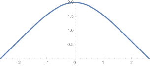
The existence of solutions of (16) follows now standard techniques of radial solutions for some equations of mean curvature type ([2, 5]). In Figure 2 we show the solutions of (16) when is positive and negative.

Theorem 3.2.
The initial value problem (16) has a solution for some that depends continuously on the initial data.
Proof.
In order to find a fixed point of , we prove that is a contraction in for some to be chosen. The functions and are locally Lipschitz continuous of constant in and respectively, provided . Since , then . Then for all and for all ,
By choosing small enough, we deduce that is a contraction in the closed ball . Thus the Schauder Point Fixed Theorem proves the existence of one fixed point of , so the existence of a local solution of the initial value problem (16). This solution belongs to . The -regularity up to is verified directly by using the L’Hôpital rule because (14) leads to
that is,
| (17) |
The continuous dependence of local solutions on the initial data is a consequence of the continuous dependence of the fixed points of . ∎
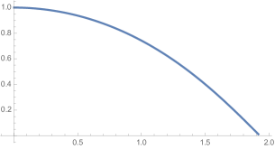
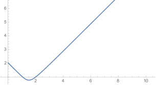
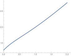
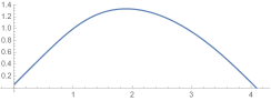
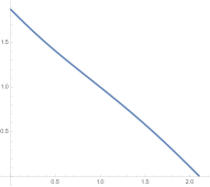
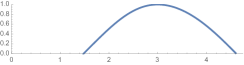
In the following result we describe the geometric properties of the rotational solutions of (15). See figures 2, 3 and 4.
Theorem 3.3.
Let be a solution of (14) with and .
-
1.
Case . The maximal domain of is . Let . Then we have the following cases: and the function is increasing; and has a unique critical point which is a global minimum; and the function is increasing. In all cases,
(18) Also, the function is a solution of (14).
-
2.
Case . The maximal domain of is with and
If , then has a global maximum and
If , let . Then we have the following cases: and is a decreasing function; and is a decreasing function; and has a global maximum.
Proof.
We observe that if has a critical point at , then (15) implies , hence all critical points are all maximum or are all minimum. Thus there is one critical point at most. In such a case, this point is a global minimum (resp. maximum) if (resp. ).
Claim A. If the graphic of meets the -axis at , then and .
The proof follows by multiplying (15) by and integrating. Then
In a neighborhood of , the right-hand side of the above equation is finite. Since as , the same occurs with , proving that as . Moreover, the case is not possible because the left-hand side would be .
Claim B. If the graphic of meets the -axis, then or .
Let denote . From Theorem 3.2, we know the existence of solutions when . Suppose now . By contradiction, we assume that . For close to and by (16),
| (19) |
Since , letting we have
Letting and by the L’Hôpital rule, we deduce
hence , a contradiction.
In particular, the claim B implies that it is not possible to find solutions of the initial value problem (16) when .
From now, we will denote by and (similar for ), the limit of and at .
Claim C. If (resp. ), then (resp. ).
Suppose that (similarly for ). If , then is bounded around by (15). Since and are bounded functions, we could extend the solution beyond , a contradiction.
We are in position to prove the theorem.
-
1.
Case . Suppose that in all its domain. Since and are bounded functions by (15), then the value of in is . If , this implies that by Claim C and this a contradiction by Claim A. This proves that .
Suppose that the sign of is negative in all its domain. Then (15) implies that is a concave function and thus because is decreasing. Then , which is not possible by Claim A.
After the above arguments, we have proved that if has a constant sign, then , and either or . In case that changes of sign, then there is a unique critical point at some point , which is a global minimum. In this case, for . Since and are bounded, then . The case is forbidden by Claim C. Thus . Since for , Claim B asserts .
We prove (18). Since is increasing close , let . If , then as and using (15), , a contradiction. Thus .
Finally, by a direct computation, we observe that is a solution of (14).
-
2.
Case . Suppose that in all its domain. Let . If , then and (15) would imply that is either if or if , a contradiction. Thus , hence . By Claim A, . If , then because is decreasing: a contradiction by Claim C. Thus . By Claim B and because is decreasing, we have two possibilities, namely, and .
Suppose now that in all its domain. Then is a concave function by (15). By Claim C, we have . In the other end of the interval , namely , we have , or , and . In both cases, as , we find and . By (19)
Letting , the left-hand side is . However, and applying twice the L’Hôpital rule, the limit of the right-hand side is
obtaining a contradiction.
Thus, if at some point, there is a critical point of , which will be the global maximum of . Then with because is increasing in .
∎
Remark 3.4.
If , there exist solutions that do not meet the rotation axis, see figure 4, right. This case appears if , where the function has a global maximum and . This extends the same property of the solution of (4), where the part of the function given in (5) that lies over the -axis is formed by successive bounded intervals.
4 The Dirichlet problem
The Dirichlet problem of the singular maximal surface equation asks if given a positive function defined in a bounded domain , there exists a smooth positive function such that (9) holds in , on and on . Since any curve in a spacelike surface must be spacelike, the graph of is spacelike. The problem is to determine the type of function and the boundary for the solvability of the Dirichlet problem. It is expectable that the sign in (9) plays an important role because we have seen in Sections 2 and 3 the contrast of the behaviour of the invariant solutions of (7) depending if is positive or negative.
Following similar ideas of Jenkins and Serrin in [11, 23], we will solve the Dirichlet problem if the domain is mean convex. In fact, we will establish the Dirichlet problem in the -dimensional case, or equivalently, we will find singular maximal hypersurfaces in the -dimensional Lorentz-Minkowski space with prescribed boundary data.
Recall that a bounded domain is said to be mean convex if has nonnegative mean curvature with respect to the inward orientation. In case , the mean convexity property is equivalent to the convexity of , but in arbitrary dimensions, the mean convexity is less restrictive than convexity.
The Dirichlet problem is now formulated as follows. Let be a smooth bounded domain and a given constant. Let be a positive spacelike smooth function. The problem is finding a classical solution , in , of
| (20) |
We solve the Dirichlet problem when the boundary data has a spacelike extension in .
Theorem 4.1.
Let be a bounded mean convex domain with smooth boundary . Assume that . If is a positive function with , then there is a unique positive solution of (20).
The proof of Theorem 4.1 is accomplished by using the Schauder theory of a priori global estimates, the method of continuity and the Leray-Schauder fixed point theorem. Applying these techniques, we find all elements for proving Theorem 4.1. As usual, we will utilize the distance function to to construct a barrier function ([10, 11, 12]).
The estimates will be obtained by comparing the solution of (20) with the rotational examples studied in Section 3: here the hypothesis will be essential because if it is not possible to prevent that for a solution . For the estimates, we need to prove that is bounded away from which will be deduced by using barrier functions. Finally, the hypothesis will be also used when we apply the Implicit Function Theorem for the existence of the linearized problem associated to (20).
The maximum principle for elliptic equations of divergence type implies the following result.
Proposition 4.2 (Touching principle).
Let and be two -singular maximal surfaces. If and have a common tangent interior point and lies above around , then and coincide at an open set around .
We also need to formulate the comparison principle in the context of -singular maximal surfaces. We write the equation of (20) in classical notation. Define the operator
| (21) |
where
Here , , and we assume the summation convention of repeated indices. It is immediate that is a solution of equation (20) if and only if . The ellipticity of the operator is clear because if and , then
| (22) |
Moreover, this shows that is not uniformly elliptic. We recall the comparison principle ([10, Th. 10.1]).
Proposition 4.3 (Comparison principle).
Let be a bounded domain. If satisfy and on , then in .
Notice that if , the classical theory implies the uniqueness of solutions of the Dirichlet problem.
Proposition 4.4.
Let be a bounded domain and . The solution of (20), if exists, is unique.
In arbitrary dimension, it holds the property that any horizontal translation and any dilation from a point of preserves equation (20). Similarly, Theorem 3.3 holds where now (16) is
We establish the solvability of (20) in the particular case that is a ball of and is a positive constant.
Proposition 4.5.
Let and be a round ball of radius . If , then there is a unique radial solution of (20) in with on .
Proof.
After a horizontal translation, we suppose that the origin is the center of . By Proposition 3.2, let be the solution of (16) with . Recall that Theorem 3.3 asserts that the maximal domain of is a ball for some with . In the -plane, consider the line . Since is a decreasing function, the graph of meets this line at one point , . If , then is a solution of (20) with . ∎
Following a standard scheme, we start by finding estimates by using the rotational solutions of (7). In the following result, we do not require the mean convexity of .
Proposition 4.6.
Let be a bounded domain and . If is a positive solution of (20), there exists a constant such that
| (23) |
Proof.
Since the right-hand side of (20) is negative, then by the maximum principle. This proves the left inequality of (23).
For the upper estimate of (23), we consider the radial solution of (16) with and let where . Denote the maximal domain of , with and let denote the graph of . Take sufficiently big so the graph of is included in the domain of the halfspace bounded by . Let decrease to until the first time that meets . By the maximum principle, the first contact must occur at some boundary point of . Then this point is a point of or a point of . Since is the graph of , this value depends on and . Consequently, . The proof finishes by letting , which depends only on , and . ∎
The next step to prove Theorem 4.1 is the derivation of estimates for . This is done firstly proving the the supremum of is attained at some boundary point. In the next result, the assumption that is negative is essential.
Proposition 4.7 (Interior gradient estimates).
Let be a bounded domain and . If is a positive solution of (20), then
Proof.
Let , . By differentiating with respect to , we find for each ,
| (24) |
Equation (24) is a linear elliptic equation in . Because , the coefficient for is negative and the maximum principle ([10, Th. 3.7]) implies that , and then has not an interior maximum. In particular, the maximum of on is attained at some boundary point, proving the result. ∎
As a consequence of Proposition 4.7, the problem of finding a priori estimates of reduces to get these estimates along . With this purpose, we prove that admits barriers from above and from below along . It is now when we use the assumption of the mean convexity of .
Proposition 4.8 (Boundary gradient estimates).
Let be a bounded mean convex domain and . If is a positive solution of (20), then there is a constant
such that
Proof.
We consider the operator defined (21). For a lower barrier for , we take the solution of the Dirichlet problem of the maximal surface equation in with the same boundary . The function is the solution of (20) for whose existen is assured ([1, Th. 4.1]). Then
Since on , we conclude in by the comparison principle.
We now construct an upper barrier for by means of the distance function in a small tubular neighborhood of in .
Consider the distance function and let sufficiently small so is a tubular neighborhood of . We parametrize using normal coordinates , where for some , is the orthogonal projection and is the unit normal vector to pointing to . A straightforward computation leads to that is , , and for all . Because is mean convex, then .
Define in a function , where we use the same symbol for a spacelike extension of into . The function is defined as
| (25) |
where is the constant that appears in (23) and and will be chosen later. Let us observe that and that we require that . The computation of leads to
From , it follows that for all . If is the canonical basis of and , we find . Thus
where are the eigenvalues of , which all are not positive because is negative semidefinite. Using this inequality, the definition of in (21) and (22), it follows that
Again (22) implies and , where . Since and , we find
| (26) |
We now study the spacelike condition . The computation of and the Cauchy-Schwarz inequality gives
Because and is decreasing on , we deduce
| (27) |
where . Fix a constant with the property . Then it is possible to choose sufficiently small in (27) so . Let . If , then (26) implies
| (28) |
The right-hand side in (28) is a function defined in . Let and we evaluate this function at , obtaining
If is sufficiently big, then , hence the right-hand side in this inequality is negative. By compactness of and by continuity, let us take sufficiently large enough in (28) so . Even more, we require so large such that . We now change the tubular neighborhood by replacing by and we denote again.
In order to assure that is a local upper barrier in for the Dirichlet problem (20), we need to have
| (29) |
In , the distance function is , so . On the other hand, in , and because , we find
By Proposition 4.6, we have and we deduce in . Definitively, we find and in , concluding that in by the comparison principle.
Consequently, we have proved the existence of lower and upper barriers for in , namely, in . Hence we deduce
and both values depend only on the initial data of the Dirichlet problem. This completes the proof of proposition. ∎
With all above ingredients, we are in position to prove Theorem 4.1.
Proof of Theorem 4.1.
We establish the solvability of the Dirichlet problem (20) by the method of continuity (see [10, Sec. 17.2]). Define the family of Dirichlet problems parametrized by
where
The graph of a solution of is a -singular maximal surface. Notice that if , is the maximal surface equation and the solution of is the function that appeared in Proposition 4.8. As usual, let
The proof consists to show that . For this, we prove that is a non-empty open and closed subset of .
-
1.
The set is not empty. This is because since is the solution of .
-
2.
The set is open in . Given , we need to prove that there is an such that . Define the map for and . Then if and only if . If we show that the derivative of with respect to , say , at the point is an isomorphism, it follows from the Implicit Function Theorem the existence of an open set , with , and a function for some , such that and for all : this guarantees that is an open set of .
The proof that is one-to-one is equivalent to prove that for any , there is a unique solution of the linear equation in and on . The computation of was done in Proposition 4.7, obtaining
where are defined in (21) and
Since , and the existence and uniqueness is assured by standard theory ([10, Th. 6.14]).
-
3.
The set is closed in . Let with . For each , there exists , , such that in and in . Define the set
Then . If we prove that the set is bounded in for some , and since in (21), then Schauder theory proves that is bounded in , in particular, is precompact in (see Th. 6.6 and Lem. 6.36 in [10]). Thus there exists a subsequence converging in to some . Since is continuous, it follows in . Moreover, on , so and consequently, .
The above reasoning asserts that is closed in provided we find a constant independent of , such that
However the and estimates for the function , that is, when the parameter is , are enough as we now see.
The estimates for follow with the comparison principle. Indeed, let , , . Then and
because . Since on , the comparison principle yields in . This proves that the solutions are ordered in increasing sense according the parameter . By (23), we find
(30)
The above three steps prove the existence part in Theorem 4.1. The uniqueness is consequence of Proposition 4.4 and this completes the proof of theorem.
∎
A consequence of Theorem 4.1 is the solvability of the Plateau problem if in the following situation.
Corollary 4.9.
Let be a spacelike -submanifold of with an one-to-one orthogonal projection on the hyperplane of equation such that is the boundary of a mean convex simply-connected domain . Let . If has a spacelike extension to a graph on , then there exists a unique -singular maximal hypersurface spanning . Moreover, is a graph on .
Proof.
Theorem 4.1 asserts the existence of an -singular maximal hypersurface whose boundary is and is a graph on . Assume that is other such a hypersurface. The property that is spacelike implies that the orthogonal projection , is a local diffeomorphism between and . In particular, is a covering map and since is simply connected, the map is a diffeomorphism, in particular, is a graph on . Finally, the uniqueness of (7) when is negative concludes that . ∎
References
- [1] R. Bartnik, L. Simon, Spacelike hypersurfaces with prescribed boundary values and mean curvature. Comm. Math. Phys. 87 (1982/83), 131–152.
- [2] C. Bereanu, P. Jebelean, J. Mawhin, Radial solutions for some nonlinear problems involving mean curvature operators in Euclidean and Minkowski spaces. Proc. Amer. Math. Soc. 137 (2009), 161–169.
- [3] J. Bemelmans, U. Dierkes, On a singular variational integral with linea growth, I: Existence and regularity of minimizers. Arch. Rat. Mech. Analysis, 100 (1987), 83–103.
- [4] R. Böhme, S. Hildebrandt, E. Taush, The two-dimensional analogue of the catenary. Pacific J. Math. 88 (1980), 247–278.
- [5] Corsato, C., De Coster, C., Omari, P.: Radially symmetric solutions of an anisotropic mean curvature equation modeling the corneal shape. Discrete Contin. Dyn. Syst. Dynamical systems, differential equations and applications. 10th AIMS Conference. Suppl., 297–303 (2015).
- [6] U. Dierkes, A geometric maximum principle, Plateau’s problem for surfaces of prescribed mean curvature, and the two-dimensional analogue of the catenary. in: Partial Differential Equations and Calculus of Variations, pp. 116-141, Springer Lecture Notes in Mathematics 1357 (1988).
- [7] U. Dierkes, Minimal hypercones and minimizers for a singular variational problem. Indiana Univ. Math. J. 37 (1988), 841–863.
- [8] U. Dierkes, Singular minimal surfaces. Geometric analysis and nonlinear partial differential equations, 177–193, Springer, Berlin, 2003.
- [9] U. Dierkes, G. Huisken, The -dimensional analogue of the catenary: existence and nonexistence. Pacific J. Math. 141 (1990), 47–54.
- [10] D. Gilbarg, N. S. Trudinger, Elliptic Partial Differential Equations of Second Order. Second edition. Springer-Verlag, Berlin, 1983.
- [11] H. Jenkins, J. Serrin, The Dirichlet problem for the minimal surface equation in higher dimensions. J. Reine Angew. Math. 229 (1968),170–187.
- [12] O. A. Ladyzhenskaya, N. N. Ural’tseva, Quasilinear elliptic equations and variational problems with several independent variables. Uspehi Mat. Nauk 16 (1961), 19–90.
- [13] R. López, Timelike surfaces with constant mean curvature in Lorentz three-space. Tohoku Math. J. (2) 52 (2000), 515–532.
- [14] R. López, Differential geometry of curves and surfaces in Lorentz-Minkowski space. Int. Electron. J. Geom. 7 (2014), 44–107.
- [15] R. López, Constant mean curvature hypersurfaces in the steady state space: a survey. Lorentzian geometry and related topics, 185–212, Springer Proc. Math. Stat., 211, Springer, Cham, 2017.
- [16] R. López, Invariant singular minimal surfaces. Ann. Global Anal. Geom. 53, (2018), 521–541.
- [17] R. López, The Dirichlet problem for the -singular minimal surface equation. Arch. Math., 112 (2019), 213–222.
- [18] R. López, Uniqueness of critical points and maximum principles of the singular minimal surface equation. J. Diff. Eq. 266 (2019), 3927–3941.
- [19] R. López, Compact singular minimal surfaces with boundary. Amer. J. Math. to appear.
- [20] A. Martínez, A. L. Martínez Triviño, A Calabi’s type correspondence. Nonlinear Anal. 191 (2020), 111637, 17 pp.
- [21] J. C. C. Nitsche, A non-existence theorem for the two-dimensional analogue of the catenary. Analysis, 6 (1986), 143–156.
- [22] B. O’Neill, Semi-Riemannian Geometry with Applications to Relativity, Academic Press, San Diego, CA, 1983.
- [23] J. Serrin, The problem of Dirichlet for quasilinear elliptic differential equations with many independent variables. Phil. Trans. Royal Soc. Lond. 264 (1969), 413–496.