WUB/19-00
CP3-Origins-2019-002 DNRF90
MITP/19-010

String breaking by light and strange quarks in QCD

Abstract

The energy spectrum of a system containing a static quark anti-quark pair is computed for a wide range of source separations using lattice QCD with $N_{\mathrm{f}}=2+1$ dynamical flavours. By employing a variational method with a basis including operators resembling both the gluon string and systems of two separated static mesons, the first three energy levels are determined up to and beyond the distance where it is energetically favourable for the vacuum to screen the static sources through light- or strange-quark pair creation, enabling both these screening phenomena to be observed. The separation dependence of the energy spectrum is reliably parameterised over this saturation region with a simple model which can be used as input for subsequent investigations of quarkonia above threshold and heavy-light and heavy-strange coupled-channel meson scattering.

1 Introduction

QCD is believed to be responsible for confinement, the experimental observation that quarks are never seen as asymptotic states [1]. A full understanding of why QCD confines remains elusive. The simplest theoretical probe of the phenomenon is provided by the potential energy $V(r)$ of a system made of a static quark and anti-quark pair immersed in the QCD vacuum in a colourless combination. This energy depends on the distance between the sources, and in the Yang-Mills theory of gluons alone it grows linearly at asymptotically large separations. The rate of increase is the well-known string tension, $\sigma$. If the static sources interact with the full QCD vacuum including light-quark dynamics, pair-creation of light quarks means the system can also resemble two separately-colourless static-light mesons allowing the potential energy to saturate at large separations. This phenomenon, induced by light-quark pair creation, is termed ‘string breaking’.

Arising from purely non-perturbative effects, the static potential requires a robust method for direct determination from the QCD Lagrangian. Lattice QCD provides such a framework, but studying string breaking on the lattice is a technical and numerical challenge. The simplest approach would be to evaluate the expectation value of large Wilson loops in the QCD vacuum and observe deviation from an area law. However, Monte Carlo determinations of large loops suffer from poor signal-to-noise properties. Also, viewed in terms of eigenstates of the Lattice QCD Hamiltonian, the creation operator comprising the Wilson line forming one edge of the rectangular Wilson loop has very small overlap onto the two-meson system dominating the ground state at large separations. As a consequence, the saturation effect proves impossible to resolve from Monte Carlo studies of Wilson loops alone. Instead, a mixing analysis including two-meson ‘broken’ string states is needed [2, 3, 4, 5, 6].

In this work, by building a suitably diverse basis of creation operators, mixing between the state made by a gluonic flux tube and the broken string state resembling two static-light or static-strange mesons is investigated fully in the $N_{\mathrm{f}}=2+1$ theory on the lattice for the first time. This enables us to compute reliably the energies of the lowest three Hamiltonian eigenstates up to separations where string breaking saturation occurs. A simple parameterisation of the resulting spectrum in the breaking region is given, which should provide invaluable first-principles input into models of coupled-channel scattering of heavy-light mesons and the decays of quarkonia near threshold.

2 Methodology

We compute the potential energy of a system containing a heavy quark $Q$ at spatial position $\mathbf{x}$ and a heavy anti-quark $\bar{Q}$ at $\mathbf{y}$ in the static approximation. In this limit, the quarks remain separated by $\mathbf{r}=\mathbf{y}-\mathbf{x}$, where $\mathbf{x}$ and $\mathbf{y}$ are conserved quantum numbers. To determine the energies of the ground state as well as the first- and second-excited state arising from mixing in QCD, a variational technique is employed. The input for this mixing calculation is a matrix of temporal correlation functions between the interpolator for a Wilson line $\mathcal{O}_{W}$, the two-static-light $\mathcal{O}_{B\bar{B}}$ and the two-static-strange meson states $\mathcal{O}_{B_{s}\bar{B}_{s}}$. It is essential that the interpolators transform irreducibly under the appropriate symmetry group.

2.1 Interpolators

A suitable interpolator $\mathcal{O}_{W}$ creating a gluon string connecting sites $\mathbf{x}$ and $\mathbf{y}$ at time $t$ is given by

$$\mathcal{O}_{W}(\mathbf{y},\mathbf{x},t)\ \ =\ \ \bar{Q}(\mathbf{y},t)\frac{\bm{\gamma}\cdot\mathbf{r}}{r}\mathcal{W}(\mathbf{y},\mathbf{x},t)Q(\mathbf{x},t),$$ (2.1)

where $\bm{\gamma}$ is the three-vector of spatial Dirac matrices and the Wilson line $\mathcal{W}(\mathbf{y},\mathbf{x},t)$ is a product of spatial lattice links with time argument $t$ connecting $\mathbf{x}$ and $\mathbf{y}$. Wilson lines are constructed using a variant of the Bresenham algorithm [7] to approximate the shortest connection between $\mathbf{x}$ and $\mathbf{y}$, cf. [8]. The heavy-quark spins are coupled symmetrically via $\bm{\gamma}\cdot\mathbf{r}/r$, which has a zero component of angular momentum projected along $\mathbf{r}$. In the static limit, both the symmetric and antisymmetric combinations give an energy level in the $\Sigma_{g}^{+}$ irreducible representation of the rotation group around $\mathbf{r}$ after the heavy spins are decoupled. Decoupling the heavy spins in the two-static-meson system similarly yields a composite operator in the $\Sigma_{g}^{+}$ irrep. Details of this construction can be found in Ref. [6]. With light-quark flavours $q^{i},i=\{u,d,s\}$, suitable interpolators for a two-static-light- or two-static-strange-meson state are given by

$$\mathcal{O}_{B\bar{B}}(\mathbf{x},\mathbf{y},t)\ \ =\frac{1}{\sqrt{2}}\sum_{i=u,d} \bar{Q}(\mathbf{y},t)\gamma_{5}q^{i}(\mathbf{y},t)\ \bar{q}^{i}(\mathbf{x},t)\gamma_{4}\gamma_{5}Q(\mathbf{x},t),$$

$$\mathcal{O}_{B_{s}\bar{B}_{s}}(\mathbf{x},\mathbf{y},t)\ \ = \bar{Q}(\mathbf{y},t)\gamma_{5}q^{s}(\mathbf{y},t)\ \bar{q}^{s}(\mathbf{x},t)\gamma_{4}\gamma_{5}Q(\mathbf{x},t).$$ (2.2)

For the two-static-light-meson state, the sum projects onto the isospin-zero channel. Notice that our interpolators Eq. (2.1) contain a $\gamma_{4}$ because for the inversion of the Dirac operator we use the convention of Ref. [9].

2.2 Correlation matrix

For the $N_{\mathrm{f}}=2+1$ theory, a $3\times 3$ matrix can be constructed from the pair-wise correlations of the two isospin-zero meson-pair creation and annihilation operators in combination with the string interpolation operator

$$C(\mathbf{r},t)= \left(\begin{array}[]{ccc}\langle\mathcal{O}_{W}(t)\overline{\mathcal{O}}_{W}(0)\rangle&\langle\mathcal{O}_{B\bar{B}}(t)\overline{\mathcal{O}}_{W}(0)\rangle&\langle\mathcal{O}_{B_{s}\bar{B}_{s}}(t)\overline{\mathcal{O}}_{W}(0)\rangle\\ \langle\mathcal{O}_{W}(t)\overline{\mathcal{O}}_{B\bar{B}}(0)\rangle&\langle\mathcal{O}_{B\bar{B}}(t)\overline{\mathcal{O}}_{B\bar{B}}(0)\rangle&\langle\mathcal{O}_{B_{s}\bar{B}_{s}}(t)\overline{\mathcal{O}}_{B\bar{B}}(0)\rangle\\ \langle\mathcal{O}_{W}(t)\overline{\mathcal{O}}_{B_{s}\bar{B}_{s}}(0)\rangle&\langle\mathcal{O}_{B\bar{B}}(t)\overline{\mathcal{O}}_{B_{s}\bar{B}_{s}}(0)\rangle&\langle\mathcal{O}_{B_{s}\bar{B}_{s}}(t)\overline{\mathcal{O}}_{B_{s}\bar{B}_{s}}(0)\rangle\end{array}\right).$$ (2.6)

When mixing occurs, the above basis states are not energy eigenstates anymore and off-diagonal elements of the correlation matrix are non-vanishing. Following the method presented in [10], all gauge-links are smeared using HYP2 parameters [11, 12] $\alpha_{1}=1.0,\alpha_{2}=1.0,\alpha_{3}=0.5$, where the smearing of the temporal links amounts to a modification of the Eichten-Hill static action and propagator [13] which reduces the divergent mass renormalisation and improves the signal-to-noise ratio at large Euclidean times [12]. As a second step, we construct a variational basis for the string state using 15 and 20 levels of HYP-smeared spatial links with parameters: $\alpha_{2}=0.6,\alpha_{3}=0.3$, extending Eq. (2.6) to a $4\times 4$ matrix.

Some correlation functions in $C(\mathbf{r},t)$ include multiple light-quark field insertions. The light-quark fields must be integrated analytically prior to Monte Carlo evaluation of $C(\mathbf{r},t)$ and the resulting Wick contractions involve numerically challenging disconnected contributions. In order to calculate these contributions, and to reduce statistical variance by exploiting translational invariance of the lattice, propagators between all space-time points are needed. For this, we employ the stochastic LapH method [9]. Based on distillation [14], the method facilitates all-to-all quark propagation in a low-dimensional subspace spanned by $N_{v}$ low-lying eigenmodes of the three-dimensional gauge-covariant Laplace operator, which is constructed using stout-smeared gauge links [15] with parameters $\rho=0.1,n_{\rho}=36$. This projection onto the so-called LapH subspace amounts to a form of quark smearing, where $N_{v}$ increases in proportion to the spatial volume for a fixed physical smearing radius. Introducing a stochastic estimator in the LapH subspace in combination with dilution [16, 17] helps to reduce the rise in computational costs as the volume increases. It was shown [9] that for certain dilution schemes, the quality of the stochastic estimator remains approximately constant for increasing volume, while maintaining a fixed number of dilution projectors. The triplet $b=(T,S,L)$ specifies a dilution scheme with time $T$, spin $S$ and LapH eigenvector projector index $L$, where $F$ indicates full dilution and $In$ the interlacing of dilution projectors in index $n$. The dilution scheme and other stochastic-LapH parameters used are given in table 1.

			light		strange
Type	Dilution scheme	Source times, $t_{s}/a$	$N_{r}$	$n_{\mathrm{inv}}$	$N_{r}$	$n_{\mathrm{inv}}$
fixed	(TF,SF,LI8)	{32, 52}	5	320	2	128
relative	(TI8,SF,LI8)	{32, 33, …, 95}	2	512	1	256

Table 1: The parameters of the quark-line estimation method employed in this work. $N_{v}=192$ eigenvectors were used to form the distillation operator. Quark lines starting and terminating at the same time slice $t_{s}=t_{\!f}$ are referred to as ‘relative’, while quark lines with $t_{s}\neq t_{\!f}$ are called ‘fixed’. For definition of the LapH subspace and specification of dilution schemes, see [9]. For these schemes, a total of $32\cdot 5\cdot 2+32\cdot 2\cdot 8=832$ (light) and $32\cdot 2\cdot 2+32\cdot 8=384$ (strange) solutions of the Dirac equation are required per gauge configuration, which however can be reused for other spectroscopy projects, see e.g. [18].

2.3 Variational analysis

A correlation matrix is evaluated for a set of static-source separations $\mathbf{r}$ and time separations $t$. The energy spectrum of the system for each spatial separation can be extracted by solving a generalised eigenvalue problem (GEVP) for each $\mathbf{r}$ [19, 20],

$$C(t)\,v_{n}(t,t_{0})=\lambda_{n}(t,t_{0})\,C(t_{0})\,v_{n}(t,t_{0})\,,\quad n=1,\ldots,N\,,\quad t>t_{0},$$ (2.7)

where $\lambda_{n}$ and $v_{n}$ are the eigenvalues and eigenvectors respectively. After solving the GEVP, energies are extracted using a correlated-$\chi^{2}$ minimisation to a two-parameter, single-exponential fit ansatz.

To simplify the analysis, the GEVP is first solved for a fixed pair of time separations, $(t_{0},t_{d})$ where $t_{0}$ is a reference separation and $t_{d}$ is the diagonalisation time [21]. The correlation matrix of the resulting interpolators from this optimisation is then defined as

$$\hat{C}_{ij}(t)=\big{(}v_{i}(t_{0},t_{d}),C(t)v_{j}(t_{0},t_{d})\big{)},$$ (2.8)

where the parentheses denote an inner product over the original operator basis. A potential source of systematic error is introduced, as off-diagonal elements of $\hat{C}_{ij}$ are not exactly zero. We control this by assessing the stability of the GEVP against varying the operator basis and using different pairs $(t_{0},t_{d})$. Comparing the results for some sample distances to the GEVP as given in Eq. (2.7) shows agreement between both methods.

We are interested in the difference between the energies $V_{n}(r)$ of the ground $(n=0)$, first $(n=1)$ and second excited state $(n=2)$ and twice the energy of the static-light meson $2E_{B}$, which can be directly extracted from fits to the ratio

$$R_{n}(t)=\frac{\hat{C}_{nn}(t)}{C_{B}^{2}(t)},$$ (2.9)

of the diagonal elements of the rotated correlation matrix of Eq. (2.8) and the correlation function of a single static-light meson squared $C_{B}^{2}(t)$. The energy difference is extracted using a single-exponential fit. The fitted energies typically vary little as diagonalisation times $(t_{0},t_{d})$ or operator basis are varied.

3 Numerical results

Monte Carlo samples are evaluated on a subset of evenly-spaced configurations of the N200 CLS (Coordinated Lattice Simulations) ensemble with $N_{\mathrm{f}}=2+1$ flavours of non-perturbatively $O(a)$-improved Wilson fermions. The lattice size is $N_{t}\times N_{s}^{3}=128\times 48^{3}$ with an estimated lattice spacing of 0.064 fm and pion and kaon masses of $m_{\pi}=$ 280 MeV and $m_{K}=$ 460 MeV respectively [22]. Open temporal boundary conditions are imposed on the fields. The imprint on observables is expected to fall exponentially with distance from the boundary [23] so measurements are made on the central half of the lattice only.

Previous studies found the signal quality to be limited by the Wilson-loop correlation functions  [6], which a preliminary analysis on a subset of our data corroborated. We mitigate this issue by measuring Wilson loops on 1664 configurations, while diagrams containing light or strange propagators are evaluated on a subset of 104 samples. The Wilson loops are then averaged into 104 bins containing 16 configurations each, with the centre of the bin aligned with one entry in the 104-configuration subset.

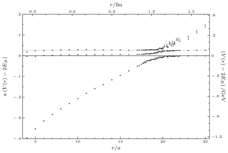
Figure 1: Static potential determined using the full mixing matrix; the three lowest lying energy levels $V_{n}(r)$, $n=0,1,2$ are shown. The grey line corresponds to twice the static-strange meson mass, its error is too small to be visible. The black line corresponds to twice the static-light meson mass; the error is automatically taken into account by using the ratio given in Eq. (2.9). For all distances, the fixed GEVP with $t_{0}/a=5,t_{d}/a=10$ is used.

For each separation $\mathbf{r}=(r_{1},r_{2},r_{3})$, we exploit cubic symmetry and average over spatial rotations to increase our statistics. As expected, no dependence on the direction is observed in our data. The analysis uses a Jupyter notebook adapted from Ref. [18]. Statistical uncertainties are estimated using 800 bootstrap resamplings [24, 25] and the uncertainty quoted is given by $1\sigma$ bootstrap errors. The covariance matrix entering the single exponential fits to Eq. (2.9) is estimated once and kept constant on every bootstrap sample.

In Fig. 1, the potential energy relative to $2E_{B}$ is shown; this subtraction removes the divergent mass renormalisation of a static quark. The grey line corresponds to twice the static-strange mass, with an energy difference $2E_{B_{s}}-2E_{B}=0.028(5)a^{-1}=85(16)$MeV. As expected due to the choice of light and strange quark masses, the difference is smaller than the physical energy difference between $B$ and $B_{s}$ mesons.

The avoided level crossing between the ground- and first-excited states is clearly visible and the expected second avoided crossing due to the formation of two static-strange mesons is also evident for the first time. As the distance over which this phenomenon occurs is small, this effect cannot be resolved using only on-axis separations [26]. For distances beyond the string breaking scale, the ground state tends rapidly towards the mass of two non-interacting static-light mesons.

The matrix of correlation functions Eq. (2.6) we use contains three very different operators, which should have strong overlap onto the three lowest physical energy eigenstates. Following Ref. [19], we expect problems with determining energies from the GEVP using a finite basis will arise when higher states for which no good operator appears in the basis are close in energy. We can estimate where the next energy levels should be around the breaking region and they are all higher by a scale of about $500$MeV, substantially larger than the gaps observed.

The string breaking region is reproduced in more detail in Fig. 2. Both avoided crossings are visible and the energy gap between the ground state and first level is larger than the gap between first and second levels. Qualitatively, the first mixing region appears to be broader, but it is not possible to determine the difference between the first string breaking distance $r_{c}$ and the second string breaking distance $r_{c_{s}}$ by eye. The quantification of string breaking involving three levels is more complex in comparison to the two-level situation. For the $N_{\text{f}}=2$ vacuum, the string breaking distance $r_{c}$ can be defined by the minimum of the energy gap $\Delta E$ [6]. When the strange quark is included, an alternative definition of the two string breaking distances $r_{c}$ and $r_{c_{s}}$ is needed as there is not necessarily a minimum energy gap.

4 A model of the string breaking spectrum

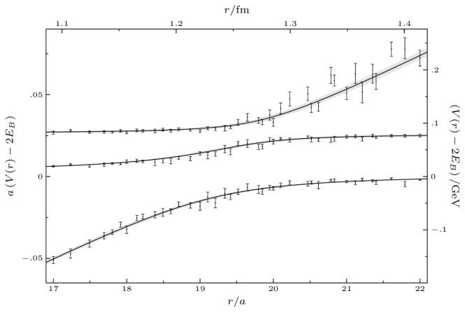
Figure 2: Six-parameter fit to the string breaking data of Fig. 1 over the fit range $r/a=[11,25]$. The error band indicates $1\sigma$ bootstrap errors.

We describe the potential-energy spectrum in the breaking region using a simple Hamiltonian that extends the model for $N_{\mathrm{f}}=2$ given in [27]. Consider a three-state system with Hamiltonian:

$$H(r)\quad= \left(\begin{array}[]{rcl}\hat{V}(r)&g_{1}&g_{2}\\ g_{1}&\hat{E}_{1}&0\\ g_{2}&0&\hat{E}_{2}\end{array}\right).$$ (4.13)

The diagonal elements are a function $\hat{V}(r)$ describing the unbroken string and $\hat{E}_{1}$, $\hat{E}_{2}$, the energies of a noninteracting pair of static-light and static-strange mesons, respectively. As with $\hat{V}$, these energies are measured relative to $2E_{B}$. $g_{1}$ and $g_{2}$ are two coupling constants describing the strength of the mixing between the gluon flux and the separated colour-screened static sources. The off-diagonal term that would mix the two-static-light-meson state with the two-static-strange-meson state is set to zero. There is no constraint on this mixing in the energy spectrum alone as a basis rotation shows any non-zero value of this parameter yields an equivalent spectrum to the Hamiltonian of Eq. (4.13). Moreover, setting this value to zero ensures the diagonal elements of $H$ correspond to the asymptotic energy eigenvalues up to corrections at ${\cal O}(r^{-1})$ in the limit $r\rightarrow\infty$.

A suitable choice for the function representing the string state is the Cornell potential [28]. Since we are modelling the string breaking region and not the potential at small distances, only the linear part of the Cornell potential

$$\hat{V}(r)=\hat{V}_{0}+\sigma r,$$ (4.14)

with string tension $\sigma$, is constrained by our data. Notice that we assume that the model parameters $\hat{E}_{1}$, $\hat{E}_{2}$, $g_{1}$ and $g_{2}$ in Eq. (4.13) are independent of the distance. We will see that this simplest possible choice models our data very well in the region of string breaking.

The eigenstates of the Hamiltonian are mixtures of the unbroken string and the two static-light- and two static-strange-meson states while the eigenvalues of $H$ correspond to the three extracted energy levels. After diagonalising $H$, we perform an uncorrelated six-parameter fit to the spectrum, whose result is shown in Fig. 2. We find for our fit parameters:

$$a\hat{E}_{1}= 0.0019(2),\hskip 28.45274pta\hat{E}_{2}=0.0262(6),$$ (4.15)

$$ag_{1}= 0.0154(4),\hskip 28.45274ptag_{2}=0.0080(5),$$

$$a^{2}\sigma= 0.0229(3),\hskip 28.45274pta\hat{V}_{0}=-0.434(5).$$

The model in Eq. (4.13) assumes a three state system. While it is possible that the physical eigenstates receive contributions from higher lying states Fig. 2 shows that our data is well-described by the fit parameters.

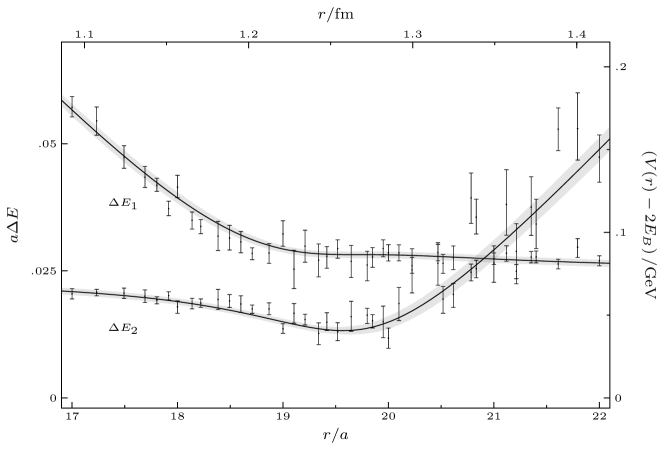
Figure 3: Energy gap between ground and first-excited state $(\Delta E_{1}(r))$, as well as first-excited and second-excited state $(\Delta E_{2}(r))$ from the model fit as well as from our data. The error band and error bars indicate $1\sigma$ bootstrap errors.

We now turn to a quantitative definition of the string breaking distance in the $N_{\mathrm{f}}=2+1$ case. To investigate the dependence of the string breaking distance on the sea quark masses, a robust definition is needed. By using the asymptotic states of our model, which for large distances $r$ are given by the diagonal entries of our Hamiltonian, we extract two distinct string breaking distances corresponding to the light and strange mixing phenomenon. The string breaking distance, $r_{c}$ associated with the formation of two static-light quarks is given by the crossing distance where $\hat{V}(r_{c})=\hat{E}_{1}$ and a corresponding definition can be employed to define $r_{c_{s}}$ using $\hat{V}(r_{c_{s}})=\hat{E}_{2}$. Our calculation yields

$$r_{c}=19.053(82)a=1.224(15)\text{fm}\ ,\ \ r_{c_{s}}=20.114(87)a=1.293(16)\text{fm}.$$ (4.16)

The quoted errors for the physical units take into account the uncertainty of $a=0.06426(76)$fm [29].

Fig. 3 shows that the energy gap $\Delta E_{1}(r)=V_{1}(r)-V_{0}(r)$ between the ground and first-excited state does not exhibit a minimum, thus making it impossible to use the minimal gap distance to define $r_{c}$. It can also be observed that in the string breaking region, $\Delta E_{1}(r)$ is twice as large as $\Delta E_{2}(r)=V_{2}(r)-V_{1}(r)$ , the energy gap between the first-excited and second-excited state.

Only one previous study [6] of string breaking for $N_{\mathrm{f}}=2$ QCD on the lattice exists with $m_{\pi}=640$MeV. However, the differing definitions and quark content of the vacua mean it is not possible to make a statement on quark mass dependence. Using the position of the minimal energy gap, they find $\hat{r}_{c}\approx 1.248(13)\text{fm}$. Even though in this study the pion mass was relatively heavy, $\hat{r}_{c}$ is of the same order of magnitude as our result and falls between our values for $r_{c}$ and $r_{c_{s}}$.

4.1 Phenomenology

To make a first, simple comparison between our data and the experimentally observed quarkonium spectrum, we use the ground-state energy computed from our model Eq. (4.13) as input potential in the Schrödinger equation and extract the bound state energies of quarkonia in the Born-Oppenheimer approximation. We use input bottom- and charm-quark masses $m_{b}=4977\,\mathrm{MeV},m_{c}=1628\,\mathrm{MeV}$ from quark models [30, 31].

$m_{Q}$	$l=0$	$l=1$	$l=2$	$l=3$	$l=4$
$m_{b}$	3	3	2	2	1
$m_{c}$	2	1	1	–	–

Table 2: Number of bound-state solutions $E_{nl}<0$ for bottomonium and charmonium of the Schrödinger equation.

The number of bottomonium bound states is listed in the first row of Tab. 2. We observe three $S$-wave states in agreement with the physical spectrum of $\Upsilon$ mesons. We do not find bound states beyond $l>4$. For the states closest to the threshold for each angular momentum, the size of the wave function as determined from the root mean-square radius is between $0.63\,r_{c}$ and $0.79\,r_{c}$. We also solved the Schrödinger equation when setting $V(r)=\min\{\sigma r+\hat{V}_{0},0\}$ and find changes in energies of less than $10\,\mathrm{MeV}$, within the errors from the fit parameters, so the bound-state spectrum is not sensitive to the width of the mixing region. The second row of Tab. 2 shows the number of bound states we find for charmonium for comparison.

This calculation is only a check that counting the bound states leads to sensible results. Our model Eq. (4.13) provides input for more refined calculations of the coupled-channel scattering of heavy-light mesons and the decays of quarkonia around threshold.

5 Conclusions

This work presents a first calculation of string breaking with $N_{\mathrm{f}}=2+1$ dynamical quarks from lattice QCD on a single ensemble with light/strange quark masses that are heavier/lighter than in nature, corresponding to $m_{\pi}=280\,\mathrm{MeV}$ and $m_{K}=460\,\mathrm{MeV}$. We compute the three lowest energy levels of a static quark and anti-quark pair and observe the avoided level crossings due to pair-creation of light and strange sea quarks. Our main result can be summarised in the model of Eq. (4.13) which provides a very good description of our spectrum, shown in Fig. 2. In particular, we extract the values of the parameters $g_{1}=47.2(1.4)\,\mathrm{MeV}$ and $g_{2}=24.5(1.6)\,\mathrm{MeV}$ which describe the mixing between the gluonic flux tube and the broken string.

Further analysis to study the dependence of string breaking on the quark masses is in progress.

References

- [1] K. G. Wilson, Confinement of Quarks, Phys. Rev. D10 (1974) 2445–2459. [,319(1974)].
- [2] I. T. Drummond, Strong coupling model for string breaking on the lattice, Phys. Lett. B434 (1998) 92–98, [hep-lat/9805012].
- [3] O. Philipsen and H. Wittig, String breaking in nonAbelian gauge theories with fundamental matter fields, Phys. Rev. Lett. 81 (1998) 4056–4059, [hep-lat/9807020]. [Erratum: Phys. Rev. Lett.83,2684(1999)].
- [4] ALPHA Collaboration, F. Knechtli and R. Sommer, String breaking in SU(2) gauge theory with scalar matter fields, Phys. Lett. B440 (1998) 345–352, [hep-lat/9807022]. [Erratum: Phys. Lett.B454,399(1999)].
- [5] ALPHA Collaboration, F. Knechtli and R. Sommer, String breaking as a mixing phenomenon in the SU(2) Higgs model, Nucl. Phys. B590 (2000) 309–328, [hep-lat/0005021].
- [6] SESAM Collaboration Collaboration, G. S. Bali, H. Neff, T. Duessel, T. Lippert, and K. Schilling, Observation of string breaking in QCD, Phys.Rev. D71 (2005) 114513, [hep-lat/0505012].
- [7] J. E. Bresenham, Algorithm for computer control of a digital plotter, IBM Systems Journal 4 (March, 1965) 25–30.
- [8] B. Bolder, T. Struckmann, G. S. Bali, N. Eicker, T. Lippert, B. Orth, K. Schilling, and P. Ueberholz, A High precision study of the Q anti-Q potential from Wilson loops in the regime of string breaking, Phys. Rev. D63 (2001) 074504, [hep-lat/0005018].
- [9] C. Morningstar, J. Bulava, J. Foley, K. J. Juge, D. Lenkner, et al., Improved stochastic estimation of quark propagation with Laplacian Heaviside smearing in lattice QCD, Phys.Rev. D83 (2011) 114505, [arXiv:1104.3870].
- [10] M. Donnellan, F. Knechtli, B. Leder, and R. Sommer, Determination of the Static Potential with Dynamical Fermions, Nucl.Phys. B849 (2011) 45–63, [[hep-lat/1012.3037]].
- [11] A. Hasenfratz and F. Knechtli, Flavor symmetry and the static potential with hypercubic blocking, Phys.Rev. D64 (2001) 034504, [hep-lat/0103029].
- [12] M. Della Morte, A. Shindler, and R. Sommer, On lattice actions for static quarks, JHEP 0508 (2005) 051, [hep-lat/0506008].
- [13] E. Eichten and B. R. Hill, An Effective Field Theory for the Calculation of Matrix Elements Involving Heavy Quarks, Phys.Lett. B234 (1990) 511.
- [14] Hadron Spectrum Collaboration Collaboration, M. Peardon et al., A Novel quark-field creation operator construction for hadronic physics in lattice QCD, Phys.Rev. D80 (2009) 054506, [arXiv:0905.2160].
- [15] C. Morningstar and M. J. Peardon, Analytic smearing of SU(3) link variables in lattice QCD, Phys.Rev. D69 (2004) 054501, [hep-lat/0311018].
- [16] W. Wilcox, Noise methods for flavor singlet quantities, in Numerical challenges in lattice quantum chromodynamics. Proceedings, Joint Interdisciplinary Workshop, Wuppertal, Germany, August 22-24, 1999, pp. 127–141, 1999. hep-lat/9911013.
- [17] J. Foley, K. Jimmy Juge, A. O’Cais, M. Peardon, S. M. Ryan, et al., Practical all-to-all propagators for lattice QCD, Comput.Phys.Commun. 172 (2005) 145–162, [hep-lat/0505023].
- [18] C. Andersen, J. Bulava, B. Hörz, and C. Morningstar, The pion-pion scattering amplitude and timelike pion form factor from lattice QCD, Nucl. Phys. B939 (2019) 145–173, [arXiv:1808.05007].
- [19] B. Blossier, M. Della Morte, G. von Hippel, T. Mendes, and R. Sommer, On the generalized eigenvalue method for energies and matrix elements in lattice field theory, JHEP 0904 (2009) 094, [arXiv:0902.1265].
- [20] M. Lüscher and U. Wolff, How to calculate the elastic scattering matrix in two-dimensional quantum field theories by numerical simulation, Nuclear Physics B 339 (1990), no. 1 222 – 252.
- [21] J. Bulava, B. Fahy, B. Hörz, K. J. Juge, C. Morningstar, and C. H. Wong, and scattering phase shifts from lattice QCD, Nucl. Phys. B910 (2016) 842–867, [arXiv:1604.05593].
- [22] M. Bruno et al., Simulation of QCD with N 2 1 flavors of non-perturbatively improved Wilson fermions, JHEP 02 (2015) 043, [arXiv:1411.3982].
- [23] M. Lüscher and S. Schaefer, Lattice QCD with open boundary conditions and twisted-mass reweighting, Comput. Phys. Commun. 184 (2013) 519–528, [arXiv:1206.2809].
- [24] B. Efron, Bootstrap methods: Another look at the jackknife, The Annals of Statistics 7 (1979), no. 1 1–26.
- [25] B. Efron and R. Tibshirani, Bootstrap Methods for Standard Errors, Confidence Intervals, and Other Measures of Statistical Accuracy, vol. 1. Institute of Mathematical Statistics, 02, 1986.
- [26] V. Koch, J. Bulava, B. Hörz, F. Knechtli, G. Moir, C. Morningstar, and M. Peardon, String breaking with 2+1 dynamical fermions using the stochastic LapH method, in 36th International Symposium on Lattice Field Theory (Lattice 2018) East Lansing, MI, United States, July 22-28, 2018, 2018. arXiv:1811.09289.
- [27] F. Knechtli, M. Günther, and M. Peardon, Lattice Quantum Chromodynamics: Practical Essentials. SpringerBriefs in Physics. Springer, 2017.
- [28] E. Eichten, K. Gottfried, T. Kinoshita, J. Kogut, K. D. Lane, and T. M. Yan, Spectrum of charmed quark-antiquark bound states, Phys. Rev. Lett. 34 (Feb, 1975) 369–372.
- [29] M. Bruno, T. Korzec, and S. Schaefer, Setting the scale for the CLS flavor ensembles, Phys. Rev. D95 (2017), no. 7 074504, [arXiv:1608.08900].
- [30] S. Capitani, O. Philipsen, C. Reisinger, C. Riehl, and M. Wagner, Precision computation of hybrid static potentials in SU(3) lattice gauge theory, Phys. Rev. D99 (2019), no. 3 034502, [arXiv:1811.11046].
- [31] S. Godfrey and N. Isgur, Mesons in a Relativized Quark Model with Chromodynamics, Phys. Rev. D32 (1985) 189–231.
- [32] SciDAC, LHPC, UKQCD Collaboration, R. G. Edwards and B. Joo, The Chroma software system for lattice QCD, Nucl. Phys. Proc. Suppl. 140 (2005) 832, [hep-lat/0409003]. [832(2004)].